SubspaceMethods
基于系统辨识下的均等化信道IIR系统(DOC)
北京化工大学北方学院毕业论文论文题目:基于系统辨识下的均等化信道IIR系统所在院系:信息院所在专业:自动化班级:自动化姓名:2012年05月11日基于系统辨识下的均等化信道IIR系统前言目前有一个新颖的方法被提议用来摸索的辨识某个未知的IIR系统。
这个方法是建立在更加快速系统输出采样基础上的,它不要求获得未知系统输入的先前统计信息和检测信号。
此方法在未知系统的参数中所呈现出的线性特征使得一些标准化的回归算法就可以容易的实现,而在本文中也明确指出:如果我们能够适过采样频率,任何一个有限序列的IIR系统都是可以确定下来的。
参考文献1.《机械工程学报》ISTICEIPK-2010年9期杨一博尹文生汪劲松朱煜蔡田YANG YiboYIN WenshengWANG JinsongZHU YuCAI Tian针对粗精动运动平台系统辨识中激励信号的生成进行了优化设计方法的研究.粗精动平台结构通常用于长行程、高精度的运动平台系统,如扫描光刻机运动平台、硬盘寻道平台等系统.获得粗精动系统的准确模型是改进粗精动运动系统。
2.《南京航空航天大学学报》ISTICEIPKU-2011年3期宋彦国孙涛Song YanguoSun Tao描述了旋翼飞行器飞行力学模型的系统辨识建模算法,从旋翼飞行器飞行动力学建模的共性问题入手,首先采用机理建模的方法分析了旋翼飞行嚣主要气动部件所受气动力.考虑旋翼挥舞运动对旋翼飞行器飞行动力学特性的影响,建立。
3.《控制理论与应用》ISTICEIPKU-2010年9期郭金库吴瑾颖刘光斌GUOJin-kuWU Jin-yingLIU Guang-bin基于信号的稀疏表示理论提出一种线性时不变系统辨识方法,该方法利用线性调频信号作为线性时不变系统激励输入信号,在利用传统方法进行系统辨识前利用稀疏分解算法对系统输出信号进行噪声处理.线性调频信号具有较好的时。
4.《机器人》ISTICEIPKU-2012年1期杜玉虎房建成盛蔚雷旭升DU YuhuFANG JianchengSHENG WeiLEI Xusheng针对小型无人直升机不稳定、强耦合、非线性的特点,建立了小型无人直升机悬停状态下飞行动力学模型.设计了一种基于最小二乘与自适应免疫遗传算法(LS-AIGA)的辨识算法,根据辨识实验的需要研制了机载微小型导航、制导与控制。
空间索引算法

空间索引算法随着科技的不断发展,数据量的急剧增加,如何高效地存储和检索数据成为了一个重要的问题。
在空间数据检索领域,空间索引算法是一种常用的解决方案。
本文将介绍空间索引算法的基本概念、分类和应用。
一、基本概念空间索引算法是一种将空间数据组织成索引结构以便快速检索的算法。
其基本思想是将空间数据划分为若干个空间单元,将数据存储在相应的单元内,并建立索引来加速检索。
空间单元的划分方式和索引结构的设计是空间索引算法的核心内容。
二、分类根据空间单元的划分方式和索引结构的设计,可以将空间索引算法分为以下几类。
1.基于网格的算法基于网格的算法是将空间数据划分为规则的网格单元,每个单元内存储相应的数据对象。
网格单元的大小可以根据数据密度和查询需求进行调整。
常见的网格单元有正方形和六边形。
基于网格的算法包括Quadtree、Octree、R-Tree等。
Quadtree是一种将空间划分为四叉树的算法,每个节点代表一个正方形空间单元。
从根节点开始,将空间逐级划分为四个子节点,直到每个节点内只包含一个数据对象。
查询时,从根节点开始递归遍历四叉树,找到与查询范围相交的节点,将其子节点加入遍历队列,直到队列为空。
Quadtree适用于二维空间数据的存储和检索。
Octree是一种将空间划分为八叉树的算法,每个节点代表一个立方体空间单元。
从根节点开始,将空间逐级划分为八个子节点,直到每个节点内只包含一个数据对象。
查询时,从根节点开始递归遍历八叉树,找到与查询范围相交的节点,将其子节点加入遍历队列,直到队列为空。
Octree适用于三维空间数据的存储和检索。
R-Tree是一种将空间划分为多维矩形的算法,每个节点代表一个矩形空间单元。
从根节点开始,将空间逐级划分为多个子节点,直到每个节点内只包含一个数据对象或者达到最大容量。
查询时,从根节点开始递归遍历R-Tree,找到与查询范围相交的节点,将其子节点加入遍历队列,直到队列为空。
R-Tree适用于多维空间数据的存储和检索。
中心刚体-柔性梁刚柔耦合动力学模型降阶研究
中心刚体-柔性梁刚柔耦合动力学模型降阶研究李莉;刘铸永;洪嘉振【摘要】The finite element method is widely used to describe the elastic deformations of flexible bodies,which leads to a large number of elastic coordinates and large computational burden.In order to reduce the degree-of-freedom of flexible bodies,a modal method and a Krylov method were used to reduce the degree-of-freedom of the flexible hub-beam system.Then the finite element model,and the reduced models based on modal method and Krylov method were used to do simulation respectively.The numerical simulations show that using the Krylov method shows faster convergence than using the modal method.It means that Krylov method is an efficient meth-od to implement model reduction of flexible multibody system.%有限单元法被广泛的采用来描述柔性体的弹性变形,然而有限元节点坐标数目庞大,将会给动力学方程求解带来巨大的计算负担。
如何降低柔性体的自由度,是当前柔性多体系统动力学研究的一个重要命题。
模幂滑动窗口法分析及加法链在预计算中的应用
模幂滑动窗口法分析及加法链在预计算中的应用屈晓;孙达志【摘要】Sliding window method is one of the most widely used methods for exponentiation, but analysis on its exact computational complexity are few. And when the window size becomes bigger, the total of precomputations grows exponentially. An analysis of the exact complexity of sliding window method with Markov transfer matrix is presented. It presents an expression of the exact complexity in binary code. The difference between theoretical and experimental values is less than 0.1time of modular multiplication. After that, a method with addition chain passing all given values in precomputation is proposed. It generates an algorithm which is computationally feasible for computer implementation. Experimental result shows that this method improves the efficiency greatly when the window size is big. This thought can also be used in the case of one message sending to many clients.%滑动窗口法是计算大数模幂问题应用最广泛的方法之一,然而针对此方法复杂度的精确理论分析却十分稀少。
量子化学方法小总结1

量子化学方法小总结12008-02-26 14:26量子化学计算方法主要分为:①分子轨道法(简称MO法);②价键法(简称VB法)。
分子轨道法,它是原子轨道对分子的推广,即在物理模型中,假定分子中的每个电子在所有原子核和电子所产生的平均势场中运动,即每个电子可由一个单电子函数(电子的坐标的函数)来表示它的运动状态,并称这个单电子函数为分子轨道,而整个分子的运动状态则由分子所有的电子的分子轨道组成(乘积的线性组合),量子计算方法主要为分子轨道常见。
分子轨道法的核心是Hartree-Fock-Roothaan方程,简称HFR方程。
1928年D.R.Hartree提出了一个将N个电子体系中的每一个电子都看成是在由其余的N-1个电子所提供的平均势场中运动的假设。
这样对于体系中的每一个电子都得到了一个单电子方程(表示这个电子运动状态的量子力学方程),称为Hartree 方程。
使用自洽场迭代方式求解这个方程,就可得到体系的电子结构和性质。
Hartree方程未考虑由于电子自旋而需要遵守的泡利原理。
1930年,B.A.Fock 和J.C.Slater分别提出了考虑泡利原理的自洽场迭代方程,称为Hartree-Fock 方程。
它将单电子轨函数(即分子轨道)取为自旋轨函数(即电子的空间函数与自旋函数的乘积)。
泡利原理要求,体系的总电子波函数要满足反对称化要求,即对于体系的任何两个粒子的坐标的交换都使总电子波函数改变正负号,而slater 行列式波函数正是满足反对称化要求的波函数。
将Hartree-Fock方程用于计算多原子分子,会遇到计算上的困难。
C.C.J.Roothaan提出将分子轨道向组成分子的原子轨道(简称AO)展开,这样的分子轨道称为原子轨道的线性组合(简称LCAO)。
使用LCAO-MO,原来积分微分形式的Hartree-Fock方程就变为易于求解的代数方程,称为Hartree-Fock -Roothaan方程,简称HFR方程。
量子力学英语词汇
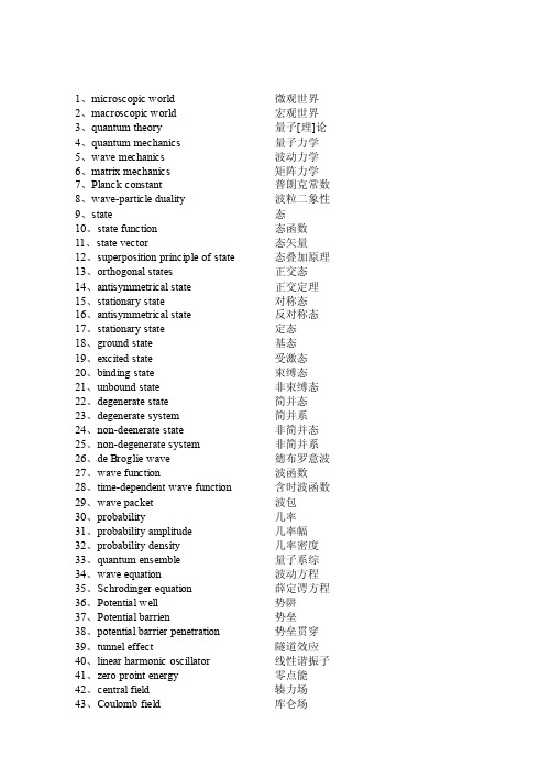
1、microscopic world 微观世界2、macroscopic world 宏观世界3、quantum theory 量子[理]论4、quantum mechanics 量子力学5、wave mechanics 波动力学6、matrix mechanics 矩阵力学7、Planck constant 普朗克常数8、wave-particle duality 波粒二象性9、state 态10、state function 态函数11、state vector 态矢量12、superposition principle of state 态叠加原理13、orthogonal states 正交态14、antisymmetrical state 正交定理15、stationary state 对称态16、antisymmetrical state 反对称态17、stationary state 定态18、ground state 基态19、excited state 受激态20、binding state 束缚态21、unbound state 非束缚态22、degenerate state 简并态23、degenerate system 简并系24、non-deenerate state 非简并态25、non-degenerate system 非简并系26、de Broglie wave 德布罗意波27、wave function 波函数28、time-dependent wave function 含时波函数29、wave packet 波包30、probability 几率31、probability amplitude 几率幅32、probability density 几率密度33、quantum ensemble 量子系综34、wave equation 波动方程35、Schrodinger equation 薛定谔方程36、Potential well 势阱37、Potential barrien 势垒38、potential barrier penetration 势垒贯穿39、tunnel effect 隧道效应40、linear harmonic oscillator线性谐振子41、zero proint energy 零点能42、central field 辏力场43、Coulomb field 库仑场44、δ-function δ-函数45、operator 算符46、commuting operators 对易算符47、anticommuting operators 反对易算符48、complex conjugate operator 复共轭算符49、Hermitian conjugate operator 厄米共轭算符50、Hermitian operator 厄米算符51、momentum operator 动量算符52、energy operator 能量算符53、Hamiltonian operator 哈密顿算符54、angular momentum operator 角动量算符55、spin operator 自旋算符56、eigen value 本征值57、secular equation 久期方程58、observable 可观察量59、orthogonality 正交性60、completeness 完全性61、closure property 封闭性62、normalization 归一化63、orthonormalized functions 正交归一化函数64、quantum number 量子数65、principal quantum number 主量子数66、radial quantum number 径向量子数67、angular quantum number 角量子数68、magnetic quantum number 磁量子数69、uncertainty relation 测不准关系70、principle of complementarity 并协原理71、quantum Poisson bracket 量子泊松括号72、representation 表象73、coordinate representation 坐标表象74、momentum representation 动量表象75、energy representation 能量表象76、Schrodinger representation 薛定谔表象77、Heisenberg representation 海森伯表象78、interaction representation 相互作用表象79、occupation number representation 粒子数表象80、Dirac symbol 狄拉克符号81、ket vector 右矢量82、bra vector 左矢量83、basis vector 基矢量84、basis ket 基右矢85、basis bra 基左矢86、orthogonal kets 正交右矢87、orthogonal bras 正交左矢88、symmetrical kets 对称右矢89、antisymmetrical kets 反对称右矢90、Hilbert space 希耳伯空间91、perturbation theory 微扰理论92、stationary perturbation theory 定态微扰论93、time-dependent perturbation theory 含时微扰论94、Wentzel-Kramers-Brillouin method W. K. B.近似法95、elastic scattering 弹性散射96、inelastic scattering 非弹性散射97、scattering cross-section 散射截面98、partial wave method 分波法99、Born approximation 玻恩近似法100、centre-of-mass coordinates 质心坐标系101、laboratory coordinates 实验室坐标系102、transition 跃迁103、dipole transition 偶极子跃迁104、selection rule 选择定则105、spin 自旋106、electron spin 电子自旋107、spin quantum number 自旋量子数108、spin wave function 自旋波函数109、coupling 耦合110、vector-coupling coefficient 矢量耦合系数111、many-partic le system 多子体系112、exchange forece 交换力113、exchange energy 交换能114、Heitler-London approximation 海特勒-伦敦近似法115、Hartree-Fock equation 哈特里-福克方程116、self-consistent field 自洽场117、Thomas-Fermi equation 托马斯-费米方程118、second quantization 二次量子化119、identical particles全同粒子120、Pauli matrices 泡利矩阵121、Pauli equation 泡利方程122、Pauli’s exclusion principle泡利不相容原理123、Relativistic wave equation 相对论性波动方程124、Klein-Gordon equation 克莱因-戈登方程125、Dirac equation 狄拉克方程126、Dirac hole theory 狄拉克空穴理论127、negative energy state 负能态128、negative probability 负几率129、microscopic causality 微观因果性本征矢量eigenvector本征态eigenstate本征值eigenvalue本征值方程eigenvalue equation本征子空间eigensubspace (可以理解为本征矢空间)变分法variatinial method标量scalar算符operator表象representation表象变换transformation of representation表象理论theory of representation波函数wave function波恩近似Born approximation玻色子boson费米子fermion不确定关系uncertainty relation狄拉克方程Dirac equation狄拉克记号Dirac symbol定态stationary state定态微扰法time-independent perturbation定态薛定谔方程time-independent Schro(此处上面有两点)dinger equation 动量表象momentum representation角动量表象angular mommentum representation占有数表象occupation number representation坐标(位置)表象position representation角动量算符angular mommentum operator角动量耦合coupling of angular mommentum对称性symmetry对易关系commutator厄米算符hermitian operator厄米多项式Hermite polynomial分量component光的发射emission of light光的吸收absorption of light受激发射excited emission自发发射spontaneous emission轨道角动量orbital angular momentum自旋角动量spin angular momentum轨道磁矩orbital magnetic moment归一化normalization哈密顿hamiltonion黑体辐射black body radiation康普顿散射Compton scattering基矢basis vector基态ground state基右矢basis ket ‘右矢’ket基左矢basis bra简并度degenerancy精细结构fine structure径向方程radial equation久期方程secular equation量子化quantization矩阵matrix模module模方square of module内积inner product逆算符inverse operator欧拉角Eular angles泡利矩阵Pauli matrix平均值expectation value (期望值)泡利不相容原理Pauli exclusion principle氢原子hydrogen atom球鞋函数spherical harmonics全同粒子identical partic les塞曼效应Zeeman effect上升下降算符raising and lowering operator 消灭算符destruction operator产生算符creation operator矢量空间vector space守恒定律conservation law守恒量conservation quantity投影projection投影算符projection operator微扰法pertubation method希尔伯特空间Hilbert space线性算符linear operator线性无关linear independence谐振子harmonic oscillator选择定则selection rule幺正变换unitary transformation幺正算符unitary operator宇称parity跃迁transition运动方程equation of motion正交归一性orthonormalization正交性orthogonality转动rotation自旋磁矩spin magnetic monent(以上是量子力学中的主要英语词汇,有些未涉及到的可以自由组合。
(完整版)量子力学英语词汇

(完整版)量子力学英语词汇1、microscopic world 微观世界2、macroscopic world 宏观世界3、quantum theory 量子[理]论4、quantum mechanics 量子力学5、wave mechanics 波动力学6、matrix mechanics 矩阵力学7、Planck constant 普朗克常数8、wave-particle duality 波粒二象性9、state 态10、state function 态函数11、state vector 态矢量12、superposition principle of state 态叠加原理13、orthogonal states 正交态14、antisymmetrical state 正交定理15、stationary state 对称态16、antisymmetrical state 反对称态17、stationary state 定态18、ground state 基态19、excited state 受激态20、binding state 束缚态21、unbound state 非束缚态22、degenerate state 简并态23、degenerate system 简并系24、non-deenerate state 非简并态25、non-degenerate system 非简并系26、de Broglie wave 德布罗意波27、wave function 波函数28、time-dependent wave function 含时波函数29、wave packet 波包30、probability 几率31、probability amplitude 几率幅32、probability density 几率密度33、quantum ensemble 量子系综34、wave equation 波动方程35、Schrodinger equation 薛定谔方程36、Potential well 势阱37、Potential barrien 势垒38、potential barrier penetration 势垒贯穿39、tunnel effect 隧道效应40、linear harmonic oscillator 线性谐振子41、zero proint energy 零点能42、central field 辏力场43、Coulomb field 库仑场44、δ-function δ-函数45、operator 算符46、commuting operators 对易算符47、anticommuting operators 反对易算符48、complex conjugate operator 复共轭算符49、Hermitian conjugate operator 厄米共轭算符50、Hermitian operator 厄米算符51、momentum operator 动量算符52、energy operator 能量算符53、Hamiltonian operator 哈密顿算符54、angular momentum operator 角动量算符55、spin operator 自旋算符56、eigen value 本征值57、secular equation 久期方程58、observable 可观察量59、orthogonality 正交性60、completeness 完全性61、closure property 封闭性62、normalization 归一化63、orthonormalized functions 正交归一化函数64、quantum number 量子数65、principal quantum number 主量子数66、radial quantum number 径向量子数67、angular quantum number 角量子数68、magnetic quantum number 磁量子数69、uncertainty relation 测不准关系70、principle of complementarity 并协原理71、quantum Poisson bracket 量子泊松括号72、representation 表象73、coordinate representation 坐标表象74、momentum representation 动量表象75、energy representation 能量表象76、Schrodinger representation 薛定谔表象77、Heisenberg representation 海森伯表象78、interaction representation 相互作用表象79、occupation number representation 粒子数表象80、Dirac symbol 狄拉克符号81、ket vector 右矢量82、bra vector 左矢量83、basis vector 基矢量84、basis ket 基右矢85、basis bra 基左矢86、orthogonal kets 正交右矢87、orthogonal bras 正交左矢88、symmetrical kets 对称右矢89、antisymmetrical kets 反对称右矢90、Hilbert space 希耳伯空间91、perturbation theory 微扰理论92、stationary perturbation theory 定态微扰论93、time-dependent perturbation theory 含时微扰论94、Wentzel-Kramers-Brillouin method W. K. B.近似法95、elastic scattering 弹性散射96、inelastic scattering 非弹性散射97、scattering cross-section 散射截面98、partial wave method 分波法99、Born approximation 玻恩近似法100、centre-of-mass coordinates 质心坐标系101、laboratory coordinates 实验室坐标系102、transition 跃迁103、dipole transition 偶极子跃迁104、selection rule 选择定则105、spin 自旋106、electron spin 电子自旋107、spin quantum number 自旋量子数108、spin wave function 自旋波函数109、coupling 耦合110、vector-coupling coefficient 矢量耦合系数111、many-particle system 多子体系112、exchange forece 交换力113、exchange energy 交换能114、Heitler-London approximation 海特勒-伦敦近似法115、Hartree-Fock equation 哈特里-福克方程116、self-consistent field 自洽场117、Thomas-Fermi equation 托马斯-费米方程118、second quantization 二次量子化119、identical particles 全同粒子120、Pauli matrices 泡利矩阵121、Pauli equation 泡利方程122、Pauli’s exclusion principle泡利不相容原理123、Relativistic wave equation 相对论性波动方程124、Klein-Gordon equation 克莱因-戈登方程125、Dirac equation 狄拉克方程126、Dirac hole theory 狄拉克空穴理论127、negative energy state 负能态128、negative probability 负几率129、microscopic causality 微观因果性本征矢量eigenvector本征态eigenstate本征值eigenvalue本征值方程eigenvalue equation本征子空间eigensubspace (可以理解为本征矢空间)变分法variatinial method标量scalar算符operator表象representation表象变换transformation of representation表象理论theory of representation波函数wave function波恩近似Born approximation玻色子boson费米子fermion不确定关系uncertainty relation狄拉克方程Dirac equation狄拉克记号Dirac symbol定态stationary state定态微扰法time-independent perturbation定态薛定谔方程time-independent Schro(此处上面有两点)dinger equation 动量表象momentum representation 角动量表象angular mommentum representation占有数表象occupation number representation坐标(位置)表象position representation角动量算符angular mommentum operator角动量耦合coupling of angular mommentum对称性symmetry对易关系commutator厄米算符hermitian operator厄米多项式Hermite polynomial分量component光的发射emission of light光的吸收absorption of light受激发射excited emission自发发射spontaneous emission轨道角动量orbital angular momentum自旋角动量spin angular momentum轨道磁矩orbital magnetic moment归一化normalization哈密顿hamiltonion黑体辐射black body radiation康普顿散射Compton scattering基矢basis vector基态ground state基右矢basis ket ‘右矢’ket基左矢basis bra简并度degenerancy精细结构fine structure径向方程radial equation久期方程secular equation量子化quantization矩阵matrix模module模方square of module内积inner product逆算符inverse operator欧拉角Eular angles泡利矩阵Pauli matrix平均值expectation value (期望值)泡利不相容原理Pauli exclusion principle氢原子hydrogen atom球鞋函数spherical harmonics全同粒子identical particles塞曼效应Zeeman effect上升下降算符raising and lowering operator 消灭算符destruction operator产生算符creation operator矢量空间vector space守恒定律conservation law守恒量conservation quantity投影projection投影算符projection operator微扰法pertubation method希尔伯特空间Hilbert space线性算符linear operator线性无关linear independence谐振子harmonic oscillator选择定则selection rule幺正变换unitary transformation幺正算符unitary operator宇称parity跃迁transition运动方程equation of motion正交归一性orthonormalization正交性orthogonality转动rotation自旋磁矩spin magnetic monent(以上是量子力学中的主要英语词汇,有些未涉及到的可以自由组合。
定义Public语句,Dim语句,Function过程,Sub过程的区别

定义Public语句,Dim语句,Function过程,Sub过程的区别
说明:
实际上窗体、报表属于比较特殊一点的类,这里为了新手看的更明白一点,将其放在和类同一概念级别。
指示Sub子过程、Function函数、类的有效范围:
Public:
范围为全局公有,在所有模块、类、窗体、报表中均可以调用。
同时可用于定义全局变量。
Private:
范围为模块私有,只能在定义它的模块/类/窗体/报表中使用。
同时可用于定义模块级变量。
Dim:
即Dimention的缩写,用来定义变量。
一般主用在Sub和Function中,模块和类模块的开头位置也可以用来定义模块级变量,但建议最好还是使用Private更准确一些。
定义子程序或函数:
Sub:
即Subroutine子程序。
用于执行一段代码完成某项任务处理,并且不需要向它的调用者返回信息。
Function:
即函数,包含Sub的所有功能,同时还能提供返回值。
例如进行某项计算,最后将计算结果返回给调用者。
krylov子空间方法的分类

krylov子空间方法的分类The Krylov subspace method is a powerful numerical technique used to solve large, sparse linear systems of equations. It is widely used in various engineering and scientific applications, including computational fluid dynamics, structural engineering, and quantum physics. Krylov subspace methods can be categorized into several different types based on their underlying principles and algorithms.Krylov子空间方法是一种强大的数值技术,用于解决大型稀疏线性方程组。
它被广泛应用于各种工程和科学应用中,包括计算流体力学,结构工程和量子物理学。
Krylov子空间方法可以根据其基本原理和算法进行几种不同类型的分类。
One way to classify Krylov subspace methods is based on the type of matrix-vector multiplication used. For example, the conjugate gradient method is a type of Krylov subspace method that uses symmetric positive definite matrices, while the generalized minimal residual method is used for non-symmetric matrices. These methods are designed to efficiently compute approximate solutions to largelinear systems by iteratively building a subspace of the Krylov space generated by the matrix.一种分类Krylov子空间方法的方法是基于使用的矩阵-向量乘法的类型。
子空间迭代法的两种Rayleigh商加速技术

南京航空航天大学硕士学位论文摘要本文研究求解大型对称矩阵特征值问题的子空间迭代法。
为了加速子空间迭代法的收敛性,我们应用Rayleigh商最小化技术得到两种新的改进算法。
第一种改进算法是用Rayleigh商加速子空间迭代法。
它用每次迭代得到的Ritz矩阵和将Ritz反迭代得到的矩阵,二者构造一个带参数矩阵的线性组合,适当选取参数矩阵,使组合后的矩阵的列向量的Rayleigh商达到最小,从而更接近最小特征向量。
第二个改进算法是用带位移的Rayleigh商加速子空间迭代法。
与第一个改进算法类似,都是构造了一个带参数矩阵的线性组合,不过它选用的矩阵不同,是用Ritz矩阵和将Ritz矩阵带位移反迭代后得到的矩阵构造的,同样通过选取适当的参数矩阵,使其Rayleigh商达到最小,从而加速子空fD】的收敛性。
本文分析了这两个改进算法中参数矩阵的选取及其性质,数值稳定性和算法的收敛性,并给出了数值实验,将新方法和原始子空间方法进行比较,数值实验表明新改进的两个算法比子空间方法更优越。
关键词:对称正定矩阵,特征值,特征向量,子空间迭代法,Rayleigh商反迭代,带位移的反迭代。
子空间迭代的两种Rayleigh商加速技术ABSTRACTInthispaper,weconsiderthesubspaceiterationmethodforsolvinglargesymmetriceigenproblems,Inordertoacceleratetheconvergencerate,weimprovetheoriginalmethodwithaccelerationtechnique,andpresenttwonewalgorithmsInmythefirstproposedalgorithm,AcombinationofthelatestmatrixreceivedbyinverseiterationandtheRitzmatrixisformedinvolvinganundeterminedparametermatrix,whichisdeterminedbyminimizingtheRayleighquotient,thenitwillneartheminimaleigenvector.Inmythesecondproposedalgorithm,Wecreateacombinationasthesameasthefirstone,butinthesecondonethecombinationinvolvinganundeterminedparametermatrix,whichisdeterminedbyminimizingtheRayleighquotientisformedbythelatestmatrixreceivedbyashiftedinverseiterationandtheRitzmatrix,thenacceleratetheconvergencerateofsubspace.Inthepaper.Weanalysisthechoosingmethodoftheparametermatrixanditssomeproperty,thenumericalstabilityandconvergence.Ournumericalresultsshowthatthetwoproposedalgorithmsaresuperiortotheoriginalsubspaceiterationmethod.Keywords:symmetricmatix,eigenvalue,eigenvector,subspaceimrationmethod’Rayleighquotient,inverseiteration,theshiftedinverseiteration。
多项式空间
多项式空间
多项式空间,又称为球空间或多项式空间(Pe)IynOmialSPace),是一种多维空间结构,由具有若干变量的多项式(POIynOmial)组成。
每个变量有各自的参数或者次数,当把它们组合起来时,就可以得到多维空间。
多项式空间也可以用来表示一个定义域上的多项式集合。
它可以提供方便的数学理论框架,来解决各种复杂的数学问题。
与标准数论中的有界空间相反,多项式空间是无界的。
在这个空间中,可以显示一个或多个变量的参数和多项式的位数之间的关系。
多项式空间有着广泛的应用,可以用来处理和解决各种复杂的统计问题。
它也可以作为一种数学建模工具,可以解决许多科学和工程领域的问题。
例如,它可以用来求解:
线拟合问题,即通过给定的一组数据,如何在指定的范围内,恰当地近似表示出一条曲线;
题规划问题,即在指定的范围内,最大化或最小化一个函数;
线性优化问题,即通过求解一个多项式系统来最大化或最小化一个函数;
值分析问题,即求解一个多元微分方程;
学计算问题,例如高精度算术操作;
维函数极值问题,即寻找一个多维函数的极值点;
像处理问题,例如图像分割,图像压缩,图像识别等;
信号处理问题,如声音混叠,音调控制,声纹识别,数字信号处
理等。
总之,多项式空间在很多学科中都具有广泛的应用,它可以提供一个有效的框架来求解各种复杂的统计问题。
子空间方法

子空间方法
子空间方法(Subspace methods)是一类矩阵分解方法,主要
用于信号处理和数据分析。
它的基本思想是将原始数据矩阵分解为多个低维子空间的线性组合,以此来提取数据的潜在结构和重要信息。
子空间方法通常包括主成分分析(PCA)、因子分析(FA)、独立成分分析(ICA)等,它们都可以通过矩阵的特征值和特
征向量来实现数据分解和降维。
在实际应用中,子空间方法可以用于信号降噪、图像处理、语音识别、机器学习等领域。
例如,在语音识别中,子空间方法可以将声音信号与噪声信号进行分离,以提高语音识别的准确性。
在机器学习中,子空间方法可以用于特征提取和数据压缩,以降低模型的复杂度和加速训练过程。
【25】Robust recovery of subspace structures by low-rank representation

Robust Recovery of Subspace Structures by Low-Rank RepresentationGuangcan Liu,Member,IEEE,Zhouchen Lin,Senior Member,IEEE,Shuicheng Yan,Senior Member,IEEE,Ju Sun,Student Member,IEEE,Yong Yu,and Yi Ma,Senior Member,IEEEAbstract—In this paper,we address the subspace clustering problem.Given a set of data samples(vectors)approximately drawn from a union of multiple subspaces,our goal is to cluster the samples into their respective subspaces and remove possible outliers as well.To this end,we propose a novel objective function named Low-Rank Representation(LRR),which seeks the lowest rank representation among all the candidates that can represent the data samples as linear combinations of the bases in a given dictionary.It is shown that the convex program associated with LRR solves the subspace clustering problem in the following sense:When the data is clean,we prove that LRR exactly recovers the true subspace structures;when the data are contaminated by outliers,we prove that under certain conditions LRR can exactly recover the row space of the original data and detect the outlier as well;for data corrupted by arbitrary sparse errors,LRR can also approximately recover the row space with theoretical guarantees.Since the subspace membership is provably determined by the row space,these further imply that LRR can perform robust subspace clustering and error correction in an efficient and effective way.Index Terms—Low-rank representation,subspace clustering,segmentation,outlier detectionÇ1I NTRODUCTIONI N pattern analysis and signal processing,an underlying tenet is that the data often contains some type of structure that enables intelligent representation and processing.So one usually needs a parametric model to characterize a given set of data.To this end,the well-known(linear) subspaces are possibly the most common choice,mainly because they are easy to compute and often effective in real applications.Several types of visual data,such as motion[1],[2],[3],face[4],and texture[5],have been known to be well characterized by subspaces.Moreover,by applying the concept of reproducing kernel Hilbert space,one can easily extend the linear models to handle nonlinear data.So the subspace methods have been gaining much attention in recent years.For example,the widely used Principal Component Analysis(PCA)method and the recently established matrix completion[6]and recovery[7]methods are essentially based on the hypothesis that the data is approximately drawn from a low-rank subspace.However, a given dataset can seldom be well described by a single subspace.A more reasonable model is to consider data as lying near several subspaces,namely,the data is considered as samples approximately drawn from a mixture of several low-rank subspaces,as shown in Fig.1.The generality and importance of subspaces naturally lead to a challenging problem of subspace segmentation(or clustering),whose goal is to segment(cluster or group)data into clusters with each cluster corresponding to a subspace. Subspace segmentation is an important data clustering problem and arises in numerous research areas,including computer vision[3],[8],[9],image processing[5],[10],and system identification[11].When the data is clean,i.e.,the samples are strictly drawn from the subspaces,several existing methods(e.g.,[12],[13],[14])are able to exactly solve the subspace segmentation problem.So,as pointed out by Rao et al.[3]and Liu et al.[14],the main challenge of subspace segmentation is to handle the errors(e.g.,noise and corruptions)that possibly exist in data,i.e.,to handle the data that may not strictly follow subspace structures. With this viewpoint,in this paper we therefore study the following robust subspace clustering[15]problem. Problem1.1(Robust Subspace Clustering).Given a set of data samples approximately(i.e.,the data may contain errors).G.Liu is with the Department of Computer Science and Engineering,Shanghai Jiao Tong University,China,the Coordinated Science Labora-tory,University of Illinois,1308West Main Street,Urbana-Champaign,Urbana,IL61801,and the Department of Electrical and ComputerEngineering,National University of Singapore.E-mail:gutty.liu@..Z.Lin is with the Key Laboratory of Machine Perception(MOE),School ofElectronic Engineering and Computer Science,Peking University,No.5Yiheyuan Road,Haidian District,Beijing100871,China.E-mail:zlin@..S.Yan is with the Department of Electrical and Computer Engineering,National University of Singapore,Block E4,#08-27,Engineering Drive3,Singapore117576.E-mail:eleyans@.sg..J.Sun is with the Department of Electrical Engineering,ColumbiaUniversity,1300S.W.Mudd,500West120th Street,New York,NY10027.E-mail:jusun@..Y.Yu is with the Department of Computer Science and Engineering,Shanghai Jiao Tong University,No.800Dongchuan Road,MinhangDistrict,Shanghai200240,China.E-mail:yyu@..Y.Ma is with the Visual Computing Group,Microsoft Research Asia,China,and with the Coordinated Science Laboratory,University of Illinoisat Urbana-Champaign,Room145,1308West Main Street,Urbana,IL61801.Manuscript received14Oct.2010;revised8Sept.2011;accepted24Mar.2012;published online4Apr.2012.Recommended for acceptance by T.Jebara.For information on obtaining reprints of this article,please send e-mail to:tpami@,and reference IEEECS Log NumberTPAMI-2010-10-0786.Digital Object Identifier no.10.1109/TPAMI.2012.88.0162-8828/13/$31.00ß2013IEEE Published by the IEEE Computer Societydrawn from a union of linear subspaces,correct the possibleerrors and segment all samples into their respective subspaces simultaneously.Notice that the word“error”generally refers to the deviation between model assumption(i.e.,subspaces)and data.It could exhibit as noise[6],missed entries[6],outliers [16],and corruptions[7]in reality.Fig.2illustrates three typical types of errors under the context of subspace modeling.In this paper,we shall focus on the sample-specific corruptions(and outliers)shown in Fig.2c,with mild concerns to the cases of Figs.2a and2b.Notice that an outlier is from a different model other than subspaces and is essentially different from a corrupted sample that belongs to the subspaces.We put them into the same category just because they can be handled in the same way,as will be shown in Section5.2.To recover the subspace structures from the data containing errors,we propose a novel method termed Low-Rank Representation(LRR)[14].Given a set of data samples,each of which can be represented as a linear combination of the bases in a dictionary,LRR aims at finding the lowest rank representation of all data jointly.The computational procedure of LRR is to solve a nuclear norm [17]regularized optimization problem,which is convex and can be solved in polynomial time.By choosing a specific dictionary,it is shown that LRR can well solve the subspace clustering problem:When the data is clean,we prove that LRR exactly recovers the row space of the data;for the data contaminated by outliers,we prove that under certain conditions LRR can exactly recover the row space of the original data and detect the outlier as well;for the data corrupted by arbitrary errors,LRR can also approximately recover the row space with theoretical guarantees.Since the subspace membership is provably determined by the row space(we will discuss this in Section3.2),these further imply that LRR can perform robust subspace clustering and error correction in an efficient way.In summary,the contributions of this work include:.We develop a simple yet effective method,termed LRR,which has been used to achieve state-of-the-artperformance in several applications such as motionsegmentation[4],image segmentation[18],saliencydetection[19],and face recognition[4]..Our work extends the recovery of corrupted data from a single subspace[7]to multiple subspaces.Compared to[20],which requires the bases ofsubspaces to be known for handling the corrupteddata from multiple subspaces,our method isautonomous,i.e.,no extra clean data is required..Theoretical results for robust recovery are provided.While our analysis shares similar features asprevious work in matrix completion[6]and RobustPCA(RPCA)[7],[16],it is considerably morechallenging due to the fact that there is a dictionarymatrix in LRR.2R ELATED W ORKIn this section,we discuss some existing subspace segmen-tation methods.In general,existing works can be roughly divided into four main categories:mixture of Gaussian, factorization,algebraic,and spectral-type methods.In statistical learning,mixed data is typically modeled as a set of independent samples drawn from a mixture of probabilistic distributions.As a single subspace can be well modeled by a(degenerate)Gaussian distribution,it is straightforward to assume that each probabilistic distribu-tion is Gaussian,i.e.,adopting a mixture of Gaussian models.Then the problem of segmenting the data is converted to a model estimation problem.The estimation can be performed either by using the Expectation Max-imization(EM)algorithm to find a maximum likelihood estimate,as done in[21],or by iteratively finding a min-max estimate,as adopted by K-subspaces[8]and Random Sample Consensus(RANSAC)[10].These methods are sensitive to errors.So several efforts have been made for improving their robustness,e.g.,the Median K-flats[22]for K-subspaces,the work[23]for RANSAC,and[5]use a coding length to characterize a mixture of Gaussian.These refinements may introduce some robustness.Nevertheless, the problem is still not well solved due to the optimization difficulty,which is a bottleneck for these methods.Factorization-based methods[12]seek to approximate the given data matrix as a product of two matrices such that the support pattern for one of the factors reveals the segmenta-tion of the samples.In order to achieve robustness to noise, these methods modify the formulations by adding extra regularization terms.Nevertheless,such modifications usually lead to non-convex optimization problems which need heuristic algorithms(often based on alternating minimization or EM-style algorithms)to solve.Getting stuck at local minima may undermine their performances, especially when the data is grossly corrupted.It will be shown that LRR can be regarded as a robust generalization of the method in[12](which is referred to as PCA in thisFig.1.A mixture of subspaces consisting of a2D plane and two1D lines.(a)The samples are strictly drawn from the underlying subspaces.(b)The samples are approximately drawn from the underlyingsubspaces.Fig.2.Illustrating three typical types of errors:(a)noise[6],which indicates the phenomena that the data is slightly perturbed around the subspaces(what we show is a perturbed data matrix whose columns are samples drawn from the subspaces),(b)random corruptions[7], which indicate that a fraction of random entries are grossly corrupted, (c)sample-specific corruptions(and outliers),which indicate the phenomena that a fraction of the data samples(i.e.,columns of the data matrix)are far away from the subspaces.paper).The formulation of LRR is convex and can be solved in polynomial time.Generalized Principal Component Analysis(GPCA)[24] presents an algebraic way to model the data drawn from a union of multiple subspaces.This method describes a subspace containing a data point by using the gradient of a polynomial at that point.Then subspace segmentation is made equivalent to fitting the data with polynomials.GPCA can guarantee the success of the segmentation under certain conditions,and it does not impose any restriction on the subspaces.However,this method is sensitive to noise due to the difficulty of estimating the polynomials from real data, which also causes the high computation cost of GPCA. Recently,Robust Algebraic Segmentation(RAS)[25]has been proposed to resolve the robustness issue of GPCA. However,the computation difficulty for fitting polynomials is unfathomably large.So RAS can make sense only when the data dimension is low and the number of subspaces is small.As a data clustering problem,subspace segmentation can be done by first learning an affinity matrix from the given data and then obtaining the final segmentation results by Spectral Clustering(SC)algorithms such as Normalized Cuts(NCut)[26].Many existing methods,such as Sparse Subspace Clustering(SSC)[13],Spectral Curvature Cluster-ing(SCC)[27],[28],Spectral Local Best-fit Flats(SLBF)[29], [30],the proposed LRR method,and[2],[31],possess such a spectral nature,so-called spectral-type methods.The main difference among various spectral-type methods is the approach for learning the affinity matrix.Under the assumption that the data is clean and the subspaces are independent,Elhamifar and Vidal[13]show that a solution produced by Sparse Representation(SR)[32]could achieve the so-called‘1Subspace Detection Property(‘1-SDP):The within-class affinities are sparse and the between-class affinities are all zeros.In the presence of outliers,it is shown in[15]that the SR method can still obey‘1-SDP.However,‘1-SDP may not be sufficient to ensure the success of subspace segmentation[33].Recently,Lerman and Zhang [34]proved that under certain conditions the multiple subspace structures can be exactly recovered via‘p(p1) minimization.Unfortunately,since the formulation is not convex,it is still unknown how to efficiently obtain the globally optimal solution.In contrast,the formulation of LRR is convex and the corresponding optimization problem can be solved in polynomial time.What is more,even if the data is contaminated by outliers,the proposed LRR method is proven to exactly recover the right row space,which provably determines the subspace segmentation results (we shall discuss this in Section3.2).In the presence of arbitrary errors(e.g.,corruptions,outliers,and noise),LRR is also guaranteed to produce near recovery.3P RELIMINARIES AND P ROBLEM S TATEMENT3.1Summary of Main NotationsIn this paper,matrices are represented with capital symbols. In particular,I is used to denote the identity matrix,and the entries of matrices are denoted by using½Á with subscripts. For instance,M is a matrix,½M ij is itsði;jÞth entry,½M i;:is its i th row,and½M :;j is its j th column.For ease of presentation,the horizontal(respectively,vertical)concate-nation of a collection of matrices along row(respectively, column)is denoted by½M1;M2;...;M k (respectively,½M1;M2;...;M k ).The block-diagonal matrix formed by a collection of matrices M1;M2;...;M k is denoted by diag M1;M2;...;M kðÞ¼M10000M20000...000M k2666437775:ð1ÞThe only used vector norm is the‘2norm,denoted by Ák k2.A variety of norms on matrices will be used.The matrix ‘0,‘2;0,‘1,‘2;1norms are defined by Mk k0¼#fði;jÞ:½M ij¼0g,Mk k2;0¼#f i:k½M :;i k2¼0g,Mk k1¼Pi;jj½M ij j,and Mk k2;1¼Pik½M :;i k2,respectively.The matrix‘1norm is defined as Mk k1¼max i;j j½M ij j.The spectral norm of a matrix M is denoted by Mk k,i.e.,Mk k is the largest singular value of M.The Frobenius norm and the nuclear norm(the sum of singular values of a matrix)are denoted by Mk k F and Mk kÃ,respectively.The euclidean inner product between two matrices is h M;N i¼trðM T NÞ,where M T is the transpose of a matrix and trðÁÞis the trace of a matrix.The supports of a matrix M are the indices of its nonzero entries,i.e.,fði;jÞ:½M ij¼0g.Similarly,its column supports are the indices of its nonzero columns.The symbol I (superscripts,subscripts,etc.)is used to denote the column supports of a matrix,i.e.,I¼fðiÞ:k½M :;i k2¼0g.The corresponding complement set(i.e.,zero columns)is I c. There are two projection operators associated with I and I c: P I and P I c.While applying them to a matrix M,the matrix P IðMÞ(respectively,P I cðMÞ)is obtained from M by setting ½M :;i to zero for all i2I(respectively,i2I c).We also adopt the conventions of using spanðMÞto denote the linear space spanned by the columns of a matrix M,using y2spanðMÞto denote that a vector y belongs to the space spanðMÞ,and using Y2spanðMÞto denote that all column vectors of Y belong to spanðMÞ.Finally,in this paper we use several terminologies, including“block-diagonal matrix,”“union and sum of subspaces,”“independent(and disjoint)subspaces,”“full SVD and skinny SVD,”“pseudo-inverse,”“column space and row space,”and“affinity degree.”These terminologies are defined in the Appendix,which can be found in the Computer Society Digital Library at http://doi. /10.1109/TPAMI.2012.88.3.2Relations between Segmentation and RowSpaceLet X0with skinny SVD U0Æ0V T0be a collection of data samples strictly drawn from a union of multiple subspaces (i.e.,X0is clean);the subspace membership of the samples is determined by the row space of X0.Indeed,as shown in[12], when subspaces are independent,V0V T0forms a block-diagonal matrix:Theði;jÞth entry of V0V T0can be nonzero only if the i th and j th samples are from the same subspace. Hence,this matrix,termed Shape Interaction Matrix(SIM) [12],has been widely used for subspace segmentation. Previous approaches simply compute the SVD of the data matrix X¼U XÆX V T X and then use j V X V T X j1for subspace segmentation.However,in the presence of outliers and corruptions,V X can be far away from V0and thus theLIU ET AL.:ROBUST RECOVERY OF SUBSPACE STRUCTURES BY LOW-RANK REPRESENTATION1731.For a matrix M,j M j denotes the matrix with theði;jÞth entry being theabsolute value of½M ij.segmentation using such approaches is inaccurate.In contrast,we show that LRR can recover V0V T0even when the data matrix X is contaminated by outliers.If the subspaces are not independent,V0V T0may not be strictly block-diagonal.This is indeed well expected since when the subspaces have nonzero(nonempty)intersections, then some samples may belong to multiple subspaces simultaneously.When the subspaces are pairwise disjoint (but not independent),our extensive numerical experiments show that V0V T0may still be close to be block-diagonal,as exemplified in Fig.3.Hence,to recover V0V T0is still of interest to subspace segmentation.3.3Problem StatementProblem1.1only roughly describes what we want to study. More precisely,this paper addresses the following problem. Problem 3.1(Subspace Recovery).Let X02I R dÂn with skinny SVD U0Æ0V T0store a set of n d-dimensional samples (vectors)strictly drawn from a union of k subspaces fS i g k i¼1of unknown dimensions(k is unknown either).Given a set of observation vectors X generated byX¼X0þE0;the goal is to recover the row space of X0or to recover the true SIM V0V T0as equal.The recovery of row space can guarantee high segmenta-tion accuracy,as analyzed in Section3.2.Also,the recovery of row space naturally implies success in error correction.So it is sufficient to set the goal of subspace clustering as the recovery of the row space identified by V0V T0.For ease of exploration,we consider the problem under three assump-tions of increasing practicality and difficulty. Assumption1.The data is clean,i.e.,E0¼0.Assumption 2.A fraction of the data samples are grossly corrupted and the others are clean,i.e.,E0has sparse column supports as shown in Fig.2c.Assumption 3.A fraction of the data samples are grossly corrupted and the others are contaminated by small Gaussian noise,i.e.,E0is characterized by a combination of the models shown in Figs.2a and2c.Unlike[14],the independent assumption on the sub-spaces is not highlighted in this paper because the analysis in this work focuses on recovering V0V T0rather than a pursuit of block-diagonal matrix.4L OW-R ANK R EPRESENTATION FOR M ATRIX R ECOVERYIn this section,we abstractly present the LRR method for recovering a matrix from corrupted observations.The basic theorems and optimization algorithms will be presented. The specific methods and theories for handling the sub-space clustering problem are deferred until Section5.4.1Low-Rank RepresentationIn order to recover the low-rank matrix X0from the given observation matrix X corrupted by errors E0(X¼X0þE0), it is straightforward to consider the following regularized rank minimization problem:minD;Erank DðÞþ Ek k‘;s:t:X¼DþE;ð2Þwhere >0is a parameter andÁk k‘indicates certain regularization strategy,such as the squared Frobenius norm (i.e.,kÁk2F)used for modeling the noise as show in Fig.2a[6], the‘0norm adopted by Cande`s et al.[7]for characterizing the random corruptions as shown in Fig.2b,and the ‘2;0norm adopted by Liu et al.[14]and Xu et al.[16]for dealing with sample-specific corruptions and outliers. Suppose DÃis a minimizer with respect to the variable D, then it gives a low-rank recovery to the original data X0.The above formulation is adopted by the recently established the Robust PCA method[7],which has been used to achieve the state-of-the-art performance in several applications(e.g.,[35]).However,this formulation impli-citly assumes that the underlying data structure is a single low-rank subspace.When the data is drawn from a union of multiple subspaces,denoted as S1;S2;...;S k,it actually treats the data as being sampled from a single subspace defined by S¼P ki¼1S i.Since the sumP ki¼1S i can be much larger than the union[k i¼1S i,the specifics of the individual subspaces are not well considered and so the recovery may be inaccurate.To better handle the mixed data,here we suggest a more general rank minimization problem defined as follows: minZ;Erank ZðÞþ Ek k‘;s:t:X¼AZþE;ð3Þwhere A is a“dictionary”that linearly spans the data space. We call the minimizer ZÃ(with regard to the variable Z)the “lowest rank representation”of data X with respect to a dictionary A.After obtaining an optimal solutionðZÃ;EÃÞ, we could recover the original data by using AZÃ(or XÀEÃ). Since rankðAZÃÞrankðZÃÞ,AZÃis also a low-rank recovery to the original data X0.By setting A¼I,the formulation(3) falls back to(2).So LRR could be regarded as a general-ization of RPCA that essentially uses the standard bases as the dictionary.By choosing an appropriate dictionary A,as we will see,the lowest rank representation can recover the underlying row space so as to reveal the true segmentation of data.So,LRR could handle well the data drawn from a union of multiple subspaces.174IEEE TRANSACTIONS ON PATTERN ANALYSIS AND MACHINE INTELLIGENCE,VOL.35,NO.1,JANUARY2013Fig. 3.An example of the matrix V0V T0computed from dependent subspaces.In this example,we create11pairwise disjoint subspaces, each of which is of dimension20and draw20samples from each subspace without errors.The ambient dimension is200,which is smaller than the sum of the dimensions of the subspaces.So the subspaces are dependent and V0V T0is not strictly block-diagonal.Nevertheless,it is simple to see that high segmentation accuracy can be achieved by using the above affinity matrix to do spectral clustering.4.2Analysis on the LRR ProblemThe optimization problem(3)is difficult to solve due to the discrete nature of the rank function.For ease of exploration, we begin with the“ideal”case that the data is clean.That is, we consider the following rank minimization problem:min Z rank ZðÞ;s:t:X¼AZ:ð4ÞIt is easy to see that the solution to(4)may not be unique. As a common practice in rank minimization problems,we replace the rank function with the nuclear norm,resulting in the following convex optimization problem:min Z Zk kÃ;s:t:X¼AZ:ð5ÞWe will show that the solution to(5)is also a solution to(4) and this special solution is useful for subspace segmentation.In the following,we shall show some general properties of the minimizer to problem(5).These general conclusions form the foundations of LRR(the proofs can be found in Appendix,which is available in the online supplemental material).4.2.1Uniqueness of the MinimizerThe nuclear norm is convex,but not strongly convex.So it is possible that(5)has multiple optimal solutions.Fortunately, it can be proven that the minimizer to(5)is always uniquely defined by a closed form.This is summarized in the following theorem.Theorem 4.1.Assume A¼0and X¼AZ have feasible solution(s),i.e.,X2spanðAÞ.Then,ZüA y Xð6Þis the unique minimizer to(5),where A y is the pseudo-inverse of A.From the above theorem,we have the following corollary which shows that(5)is a good surrogate of(4).Corollary 4.1.Assume A¼0and X¼AZ have feasible solutions.Let ZÃbe the minimizer to(5),then rankðZÃÞ¼rankðXÞand ZÃis also a minimal rank solution to(4).4.2.2Block-Diagonal Property of the MinimizerBy choosing an appropriate dictionary,the lowest rank representation can reveal the true segmentation results. Namely,when the columns of A and X are exactly sampled from independent subspaces,the minimizer to(5)can reveal the subspace membership among the samples.Let fS1;S2;...;S k g be a collection of k subspaces,each of which has a rank(dimension)of r i>0.Also,let A¼½A1; A2;...;A k and X¼½X1;X2;...;X k .Then we have the following theorem.Theorem4.2.Without loss of generality,assume that A i is a collection of m i samples of the i th subspace S i,X i is a collection of n i samples from S i,and the sampling of each A i is sufficient such that rankðA iÞ¼r i(i.e.,A i can be regarded as the bases that span the subspace).If the subspaces are independent,then the minimizer to(5)is block-diagonal:ZüZÃ10000ZÃ20000...000ZÃk2666437775;where ZÃi is an m iÂn i coefficient matrix with rankðZÃiÞ¼rankðX iÞ;8i.Note that the claim of rankðZÃiÞ¼rankðX iÞguarantees the high within-class homogeneity of ZÃi since the low-rank properties generally require ZÃi to be dense.This is different from SR,which is prone to produce a“trivial”solution if A¼X because the sparsest representation is an identity matrix in this case.It is also worth noting that the above block-diagonal property does not require the data samples to have been grouped together according to their subspace memberships.There is no loss of generality to assume that the indices of the samples have been rearranged to satisfy the true subspace memberships,because the solution produced by LRR is globally optimal and does not depend on the arrangements of the data samples.4.3Recovering Low-Rank Matrices by ConvexOptimizationCorollary 4.1suggests that it is appropriate to use the nuclear norm as a surrogate to replace the rank function in (3).Also,the matrix‘1and‘2;1norms are good relaxations of the‘0and‘2;0norms,respectively.So we could obtain a low-rank recovery to X0by solving the following convex optimization problem:minZ;Ek Z kÃþ k E k2;1;s:t:X¼AZþE:ð7ÞHere,the‘2;1norm is adopted to characterize the error term E since we want to model the sample-specific corruptions(and outliers)as shown in Fig.2c.For the small Gaussian noise as shown in Fig.2a,k E k2F should be chosen;for the random corruptions as shown in Fig.2b,k E k1is an appropriate choice.After obtaining the minimizerðZÃ;EÃÞ,we could use AZÃ(or XÀEÃ)to obtain a low-rank recovery to the original data X0.The optimization problem(7)is convex and can be solved by various methods.For efficiency,we adopt in this paper the Augmented Lagrange Multiplier(ALM)[36],[37] method.We first convert(7)to the following equivalent problem:minZ;E;JJ k kÃþ Ek k2;1;s:t:X¼AZþE;Z¼J:This problem can be solved by the ALM method,which minimizes the following augmented Lagrangian function: L¼k J kÃþ k E k2;1þtrÀY T1ðXÀAZÀEÞÁþtrÀY T2ðZÀJÞÁþ2ÀXÀAZÀE2FþZÀJ2FÁ: The above problem is unconstrained.So it can be minimized with respect to J,Z,and E,respectively,by fixing the other variables and then updating the Lagrange multipliers Y1and Y2,where >0is a penalty parameter.The inexact ALM method,also called the alternating direction method,isLIU ET AL.:ROBUST RECOVERY OF SUBSPACE STRUCTURES BY LOW-RANK REPRESENTATION175。
子空间,基和向量空间的联系
子空间、基和向量空间之间存在密切的联系。
1. 基(basis)是向量空间中的一组线性无关的向量,可以表示该空间中的所有向量。
换句话说,任何一个向量都可以被基中的向量线性表示。
基的维度是相同的,不同的基所含向量的个数称为维数。
向量的坐标是在基下的唯一表示,不同的基下,向量的坐标表示也会不同。
2. 子空间(subspace)是指由向量构成的非空集合,它具有封闭性,即子空间中任意的向量加法和标量乘法都是封闭的。
任何向量空间都可以被它的子空间所覆盖,因此子空间在某种程度上描述了向量空间的特性。
3. 向量空间(vector space)是一个具有加法和标量乘法两种运算的数学结构,它可以是有限维的,也可以是无限维的。
例如,R^n就是一个n维向量空间,包含了所有n维向量。
总的来说,基、子空间和向量空间是相互关联的。
基是向量空间中一组线性无关向量的集合,它构成了该空间的元素在加法和标量乘法下的基础。
子空间是由一组向量构成的非空集合,它具有封闭性。
而向量空间是一个数学结构,它具有加法和标量乘法两种运算,可以是有限维的,也可以是无限维的。
java乔列斯分解法
java乔列斯分解法java分解法又叫平方根法,是求解对称正定线性方程组最常用的方法之一。
对于一般矩阵,为了消除LU分分解概念:假定我们能把矩阵A写成下列两个矩阵相乘的形式:A=LU,其中L为下三角矩阵,U为上三角矩阵。
这样我们可以把线性方程组Ax= b写成 Ax= (LU)x = L(Ux) = b。
令Ux = y,则原线性方程组Ax = b可首先求解向量y 使Ly = b,然后求解 Ux = y,从而达到求解线性方程组Ax= b的目的。
LU分解的基本思想将系数矩阵A转变成等价的两个矩阵L和Ujava分解法(转载)_java的博客java分解java分解法又叫平方根法,是求解对称正定线性方程组最常用的方法之一。
对于一般矩阵,为了消除LU分解的局限性和误差的过分积累,采用了选主元的方法,但对于对称正定矩阵而言,选主元是不必要的。
java分解公式_无比机智的永哥的博客_乔勒斯基分解乔累斯基分解公式简介LLT分解证明具体解法稳定性LDLT分解证明具体解法例子LLT分解LDLT分解引用矩阵的三角分解是求解线性方程组常用的方法,包括LU分解,LDU分解,杜利特(Doolittle)分解,克劳特(Crout)分解,LLT(乔累斯基java)分解。
通过var模型获得残差的协方差计算,利用乔里斯基方差分解技术进一步将其转换为下三角矩阵,可以用于计算变量间的风险溢出效应使用 java分解的矩阵求逆:根据其(下三角)java 分解,求矩阵 X 的逆。
matlab开发求矩阵 X 的逆矩阵,给定它的(下三角)java 分解;即 X = LL',根据论文“java使用分解的矩阵求逆”,Aravindh Krishnamoorthy,Deepak Menon,arXiv:1111.4144。
求解为: 前面的两个的求解很简单,对于第三个求解的过程java分解法又叫平方根法,是求解对称正定线性方程组最常用的方法之一。
- 1、下载文档前请自行甄别文档内容的完整性,平台不提供额外的编辑、内容补充、找答案等附加服务。
- 2、"仅部分预览"的文档,不可在线预览部分如存在完整性等问题,可反馈申请退款(可完整预览的文档不适用该条件!)。
- 3、如文档侵犯您的权益,请联系客服反馈,我们会尽快为您处理(人工客服工作时间:9:00-18:30)。
Algorithm
– Goal: Given X, Y find wx, wy that maximizes the correlation btwn x', y'
ρ=
E[ x′y′] E[ x′2 ]E[ y′2 ] = E[w x T x y T w y ] E[w x T x x T w x ]E[w y T y y T w y ] = w xT X YTw y
(w
T x
X XT w x )( w y T Y Y T w y )
– XXT = Cxx, YYT = Cyy : within-set cov. , XYT = Cxy : between set cov. – Solutions for wx, wy by generalized eigenvalue problem or SVD
– Φ(.): nonlinear mapping to a high dimensional space – Mercer kernels can be decomposed into dot product
K(x,y) = Φ(x)Φ(y)
Kernel PCA
– Xdxn (cols of d-vectors) → Φ(X) (high dimensional vectors) – Inner-product matrix = Φ TΦ Φ(X) Φ(X) = [K(xi,xj)] ≡ Knxn(X,X) – First k eigenvectors e: transform matrix Enxk = [e1…ek] – The ‘real’ eigenvectors are Φ(X)E – New pattern y is mapped (into prin. components) by
CCA Example
X: training images, Y: corresponding pose params (pan, tilt) = (φ,θ)
First 3 principle components, parameterized by pose (φ,θ)
First 2 CCA factors, parameterized by pose (φ,θ)
– General independent bases
If k=d, Q is obtained by solving linear system if k<d, do some optimization (e.g., least squares)
Different criterion for selecting U leads to different subspace methods
– Two sets of vectors X = [x1…xm], Y = [y1…yn] – X, Y: measured from the same semantic object (physical phenomenon) – projection for each of the sets: x' = wxx, y' = wyy
Taking the top k vector pairs Wx=(wx1…wxk), Wy=(wy1…wyk), correlation matrixkxk of the projected k-vectors x', y' is diagonal th diagonals maximized k ≤ min(m,n)
With fixed sample size, the classification performance decreases as the number of feature increases
Example: Appearance-based methods (vs model-based)
Subspace and Kernel Methods
April 2004 Seong-Wook Joo
Motivation of Subspace Methods
Subspace is a “manifold” (surface) embedded in a higher dimensional vector space
References
Overview
– H. Bischof and A. Leonardis, “Subspace Methods for Visual Learning and Recognition”, ECCV 2002 Tutorial slides http://www.icg.tu-graz.ac.at/~bischof/TUTECCV02.pdf http://cogvis.nada.kth.se/hamburg-02/slides/UOLTutorial.pdf (shorter version) H. Bischof and A. Leonardis, “Kernel and subspace methods for computer vision” (Editorial), Pattern Recognition, Volume 36, Issue 9, 2003 Baback Moghaddam, “Principal Manifolds and probabilistic Subspaces for Visual Recognition”, PAMI, Vol 24, No 6, Jun 2002 (Introduction section) A. Jain, R. Duin, J. Mao, “Statistical Pattern Recognition: A Review”, PAMI, Vol 22, No 1, Jan 2000 (section 4: Dimensionality Reduction) A. Hyvrinen and E. Oja, “Independent component analysis: algorithms and applications”, Neural Networks, Volume 13, Issue 4, Jun 2000 /science/journal/08936080 T. Melzer, M. Reiter and H. Bischof, “Appearance models based on kernel canonical correlation analysis”, Pattern Recognition, Volume 36, Issue 9, 2003 /science/journal/00313203
Linear Subspaces
≈
Xdxn Udxk Qkxn
xi ≈ ∑b=1..k qbi ub
Definitions/Notations
– Xdxn: sample data set. n d-vectors – Udxk: basis vector set. k d-vectors – Qkxn: coefficient (component) sets. n k-vectors
CCA
– – – Supervised Separate (orthogonal) linear bases for each data set Transformed variables’ correlation matrix is ‘maximized’
Kernel Methods
Kernels
– Visual data is represented as a point in a high dimensional vector space – Constraints in the natural world and the imaging process causes the points to “live” in a lower dimensional subspace
Note: k could be up to d, in which case the above is a “change of basis” and ≈ → = Selection of U
– Orthonormal bases
Q is simply projection of X onto U: Q = UT X
(Φ(X)E)T Φ(y) = ET Φ(X)T Φ(y) = ET Knx1(X,y)
– The “trick” is to somehow use dot products wherever Φ(x) occurs
Exists kernel versions of FDA, ICA, CCA, …
– Non-Gaussianity measures
Kurtosis (a 4th order stat), Negentropy
ICA Examples
Natural images Faces (vs PCA)
CCA (Canonical Correlation Analysis)
Assumption, Notation
ICA (Independent Component Analysis)
Assumption, Notation
– Measured data is a linear combination of some set of independent signals (random variables x representing (x(1)…x(d)) or row d-vectors) – xi = ai1s1 + … + ainsn = ai S (ai : row n-vector) – zero-mean xi , ai assumed – X = AS (Xnxd: measured data, i.e., n different mixtures, Anxn: mixing matrix, Snxd: n independent signals)
