Critical Path Method Applied
项目管理中的进度控制方法

项目管理中的进度控制方法在项目管理中,进度控制是确保项目按计划完成的关键因素之一。
通过有效的进度控制,项目经理可以及时识别项目进展的偏差,并采取相应措施进行调整。
本文将介绍几种常见的项目进度控制方法,以帮助项目经理更好地管理项目。
一、关键路径法(Critical Path Method,简称CPM)关键路径法是一种基于网络图的进度控制方法。
首先,项目经理需要绘制出项目的网络图,明确项目中活动的先后顺序和时长。
然后,通过计算每个活动的最早开始时间、最早完成时间、最晚开始时间和最晚完成时间,确定项目的关键路径。
关键路径上的活动决定了整个项目的最短工期,项目经理需要重点关注这些活动,确保其按时完成。
二、里程碑法(Milestone Method)里程碑方法是一种基于时间节点的进度控制方法。
项目经理根据项目计划中设定的重要里程碑,制定相应的工作计划和进度安排。
每当达到一个里程碑时,项目团队和相关利益相关方可以评估项目进展情况,并及时采取必要的措施。
里程碑法强调时间节点的重要性,有助于提醒项目团队关注项目进度,并及时调整工作计划。
三、甘特图法(Gantt Chart Method)甘特图法是一种以时间为基准的进度控制方法。
通过绘制甘特图,项目经理可以清晰地看到项目中每个活动的计划开始时间、计划完成时间和实际完成时间。
甘特图上的条形代表活动的持续时间,通过条形的长度和位置,可以直观地了解项目的进展情况。
项目经理可以根据甘特图的信息,及时调整资源分配和工作计划,保持项目进度的控制。
四、进度绩效指数法(Schedule Performance Index,简称SPI)进度绩效指数是一种通过比较实际完成进度和计划完成进度之间的差异,评估项目进展情况的方法。
项目经理可以通过计算SPI值,了解项目的进度偏差程度。
SPI值小于1表示项目进度滞后,大于1表示项目进度超前。
项目经理可以根据SPI值的变化趋势,判断项目的进展是否符合预期,从而采取相应的措施进行调整。
criticalpath method
criticalpath methodCritical Path Method (CPM) 是一种项目管理技术,主要用于计划和控制项目的进度。
它通过确定项目中关键路径的活动,来预测和控制项目的总持续时间。
关键路径上的活动对项目的完成时间有直接影响,因此,必须按照规定的时间表进行。
CPM 的主要步骤包括:确定项目目标:明确项目的目标,以及实现这些目标所需的活动。
绘制网络图:根据活动之间的逻辑关系,绘制出项目的网络图。
网络图是一个包含所有活动及其相互关系的图表。
确定关键路径:关键路径是从项目开始到结束的一系列活动,这些活动的总时间是项目的总持续时间。
关键路径上的活动不能延误,否则会影响整个项目的完成时间。
制定项目计划:基于关键路径和其他非关键路径的活动,制定项目计划。
项目计划应包括每个活动的开始和结束时间,以及必要的资源和预算。
监控和控制项目进度:根据项目计划,监控和控制项目进度。
如果关键路径上的活动发生延误,需要重新评估整个项目计划。
调整项目计划:在项目执行过程中,可能需要对项目计划进行调整。
这通常是由于关键路径上的活动延误或其他未预见的问题。
CPM 的优点包括:资源优化:通过识别关键路径上的活动,可以更有效地分配资源。
预测和控制:CPM 可以预测项目的总持续时间,并在项目执行过程中进行有效的控制。
风险管理:通过识别关键路径,可以预见潜在的问题并采取措施防止或减轻风险。
然而,CPM 也有一些局限性。
例如,它主要关注时间管理,而可能忽略其他重要的项目管理要素,如成本、质量和风险。
此外,确定关键路径的主观性也可能影响结果的准确性。
NEAR-CRITICAL PATH ANALYSIS A TOOL FOR PARALLEL PROGRAM OPTIMIZATION

Proceedings of the First Southern Symposium on ComputingThe University of Southern Mississippi, December 4-5, 1998NEAR-CRITICAL PATH ANALYSIS: A TOOL FOR PARALLEL PROGRAM OPTIMIZATION CEDELL A. ALEXANDER*, ARIC B. LAMBERT†, DONNA S. REESE†,JAMES C. HARDEN†AND RON B. BRIGHTWELL‡Abstract. Program activity graphs (PAGs) can be constructed from timestamped traces of appropriate execution events. Information about the activities on the k longest execution paths is useful in the analysis of parallel program performance. In this paper, four algorithms for finding the near-critical paths of PAGs are compared. A framework for using the near-critical path information is also described. The framework includes statistical summaries and visualization capabilities that build upon the foundation of existing performance analysis tools. Within the framework, guidance is provided by the Maximum Benefit Metric, which uses near-critical path data to predict the maximum overall performance improvement that may be realized by optimizing particular critical path activities.1.Introduction. Developing efficient parallel programs has proven to be a difficult task. Substantial research has been devoted to many aspects of the problem; active work spans the computer science spectrum from algorithmic techniques, programming paradigms, advanced compilers, and operating systems to architectures and interconnection networks. Complex interactions at each of these levels have provided motivation for a suite of performance measurement and analysis tools.Insight into a system's dynamic behavior is a prerequisite for high-productivity optimization of parallel programs. Multiple tools, offering varying perspectives, may be required to gain the necessary insight. The IPS Parallel Program Measurement System [1] and the Pablo Performance Analysis Environment [2] are two significant toolkits facilitating different viewpoints based on timestamped probe descriptions of run-time events.IPS provides a hierarchy of statistical information based on a five layer model consisting of the whole program, machine, process, procedure, and primitive activity levels. Critical path and phase behavior analysis techniques guide the search for performance problems. Critical path analysis focuses the optimization effort by identifying the activities on the longest execution path; to improve the program's performance, the duration of activities on the critical path(s) must be shortened.Pablo is a visualization and sonification toolkit designed to be a de facto standard through a philosophy of portability, scalability, and extensibility. Custom performance analysis environments are constructed by graphically interconnecting a set of analysis and display modules. The graphical programming model encourages experimental exploration of the performance data.The utility of critical path analysis can be extended when information is available about the k longest paths. Optimization of specific critical path activities may provide little overall performance improvement if the second, third, etc., longest paths are of similar duration and consist of independent activities. Near-critical paths can be used to further refine the analysis process by quantifying the benefit of optimizing critical path activities. The initial focus of this paper is on efficient algorithms for determining the near-critical paths of program activity graphs. Efficient algorithms are important because program activity graphs can be very large (hundreds of thousands of vertices).We also present a framework for using near-critical path data that encompasses both statistical summaries (patterned after IPS) and the visualization capabilities of Pablo. Guidance is provided by the Maximum Benefit Metric, which includes the synergistic effects of common activities on near-critical paths *IBM's Networking Hardware Division, P.O. Box 12195, Research Triangle Park, NC 27709.†NSF Engineering Research Center for Computational field Simulation, Mississippi State University, P.O. Box 6176, Mississippi State, MS 39762.‡Sandia National Laboratories, P.O. Box 5800, Albuquerque, NM 87185-1110.2ALEXANDER, LAMBERT, REESE,HARDEN AND BRIGHTWELLto predict the maximum overall performance improvement associated with optimization of particular critical path activities.In Section 2, critical path algorithms are reviewed to provide the background needed for description of near-critical path algorithms in Section 3. Probe acquisition and construction of program activity graphs are discussed in Section 4. A framework for near-critical path analysis is presented in Section 5. Section 6 contains the description of the applications and performance results from the Maximum Benefit Metric. The paper is concluded in Section 7 with a summary of key results.2. Critical Path Algorithms.2.1. Program Activity Graphs. A program activity graph (PAG) is an acyclic, directed multigraph representing the duration and precedence relationships of program activities. Edges represent execution activities, weights represent activity durations, vertices mark activity boundaries, and outgoing activities from a vertex cannot begin until all incoming activities have completed. Multigraphs are distinguished by multiple edges between a given pair of vertices. Although not all PAGs are multigraphs, generality requires that near-critical path algorithms accommodate multigraphs (PAG characteristics are determined by the semantics of the target system). The biggest impact of the multigraph characteristic is on data structure selection.2.2. Longest Path Algorithm. IPS employs a modified shortest path algorithm, based on the diffusing computation paradigm [3], to find the path with the longest execution duration. A diffusing computation on a graph begins at the root vertices and diffuses to all descendant vertices. In the synchronous variation, a vertex will not diffuse a computation to its descendants until all incoming computations are received. A version of the synchronous algorithm with adaptations to accommodate multigraphs is given in [4].2.3. Critical Path Method. The critical path method is an operational research algorithm for finding the longest path(s) through an activity-on-edge network [5]. The critical path method calculates early start and earl) finish times for each activity in a forward pass through the network. Late start times, late finish times, and slack values are calculated in a backward pass. Table 1 defines the terms that will be used to explain the algorithm.T ABLE1. Critical Path Method NotationThe early start time of an activity is the earliest possible time the activity can begin. The late start time of an activity is the latest time the activity can start without extending the overall network completion time. The slack values are criticality measures. The total slack of an activity is the amount of time that it can be delayed without affecting the overall completion time. Activities with zero total slack are on a critical path. The free slack of an activity is the amount of time the activity can be delayed without affecting the early start time of any other activity. The total slack values of activities on a path are not independent; delaying an activity longer than its free slack reduces the slack of subsequent activities. The values calculated by the critical path method for a simple example network are shown in Fig. 1.2.4. Algorithm Comparison. The longest path algorithm is more efficient than the critical path method (since the longest path is found in a single pass through the edges). However, the critical path method produces more information; multiple critical paths are identified and the slack criticality measures are provided. Both algorithms have the same asymptotic time complexity, in 0(e), where e is the number of edges in the graph. Selection of the most appropriate algorithm is dependent upon application needs.NEAR-CRITICAL PATH ANALYSIS: A TOOL FOR PARALLEL PROGRAM OPTIMIZATION 33. Near-Critical Path Algorithms.Definition 1: A near-critical path is a path whose duration is within a certain percentage, the near-criticality percentage, of the critical path duration. The near-criticality percentage (denoted nc%) may be specified by the user or reported by the algorithm. Three near-critical path algorithm approaches are summarized in the following list:1) Specify maximum number of longest paths to find, k , and report nc% of k th longest path,2) Specify nc% and find all near-critical paths.3) Specify both k and nc% (i.e., find up to k longest near-critical paths).In this section, four near-critical path algorithms are compared: the path enumeration and extended longest path algorithms are examples of approach 1); the branch-and-bound algorithm is based on approach2); and the best-first search algorithm employs approach 3). Approach 3) can be advantageous, relative to approach 1), when the number of near-critical paths is less than k .3.1. Path Enumeration and Extended Longest Path Algorithms. An algorithm for listing the k shortest paths between two vertices of an acyclic digraph is described in [6]. The algorithm can be easily modified to enumerate longest paths. For a multigraph containing n vertices and e edges, the worst-case time and memory requirements of the algorithm are in O(kne) and O(kn 2+e), respectively.A more straightforward approach is to simply extend the longest path algorithm to find the k longest paths as described in [4]. Since the extended algorithm maintains an array of k (fixed-size) path description records for each vertex, and a descriptor is required to represent each edge, the storage requirements are in O(kn+e). The worst-case time complexity of the algorithm is in 0(ke).3.2. Brunch-and-Bound Algorithm. Brute-force depth-first searches can solve the longest path problem in linear space; however, the time complexity is exponential [7]. Branch-and-bound (BnB) is a technique that may significantly improve the efficiency of depth-first searches by eliminating unproductive search paths [8]. In this subsection, we show how the slack values calculated by the critical path method can be used as the basis for a BnB near-critical path algorithm. The notation employed to explain the algorithm is defined in Table 2.To find the critical and near-critical paths, depth-first searches are started at the root vertices. A search is terminated when either a leaf vertex is reached or max_path_duration is less than min_ncp_duration. If a leaf vertex is reached, then a critical or near-critical path has been found (FS_sum = 0 for a critical path).F ig. 2.1. C ritic al path m ethod exam ple.F IG . 1. Critical path method example.4ALEXANDER, LAMBERT, REESE,HARDEN AND BRIGHTWELLT ABLE 2. Near-Critical Path NotationThe performance of the algorithm is highly dependent upon the input PAG. In the best case, the time complexity is in 0(1). If we optimistically assume that only one edge exists between any two vertices and that no vertex has more than two outgoing edges (which is true for the PAGs that we generate), the worst-case complexity, based on the number of edges that must be examined, is in 0(1.62n). When the critical path method is also included in the analysis, the best-case and worst-case time complexities are in 0(e) and 0(1.62n+e), respectively.3.3. Best-First Search Algorithm. The slack values provided by the critical path method can also be used as the basis for a best-first search (BFS) algorithm that traverses the k longest near-critical paths in order of nonincreasing duration. The algorithm begins by evaluating all outgoing edges from root vertices. The edge with minimum total slack is selected. The critical path method guarantees that at least one of these edges will be on a critical path and have zero total slack. Once a path has been selected, traversal is an iterative process of following the edge with minimum total slack at each descendant vertex. When a leaf vertex is reached, the next longest path is selected for traversal.Traditionally, the applicability of BFS has been limited by an exponential memory requirement [9]. The memory is needed to save the state of all partially explored paths so that optimal selections can be made. Slack values provide the information needed to overcome this limitation. Since slack is a global criticality measure, storage can be constrained to maintaining state for the k longest near-critical paths that have been found. To maintain this state information, partial paths encountered during near-critical path traversal must be evaluated. Partial paths are formed by edges that are not on the current near-critical path. Partial path evaluation is based on the cost function (FS_sum + TS), and state is maintained for the minimum cost near-critical paths.To minimize path evaluation overhead, path costs are maintained in a max-heap data structure. This allows direct access to the maximum cost partial path and a new (lower) maximum can be established in logarithmic time. To minimize the overhead of selecting the next longest path, path costs are also maintained in a min-heap. When the max-heap is modified by sifting down a new entry, the associated min-heap entry is percolated up to maintain the integrity of the dual heaps. Thus, the minimum cost partial path is always available at the top of the min-heap.Path state information is preserved in path_descriptor records. Pointers to the descriptors of edges on near-critical paths are recorded in path_entry records. Paths consist of two segments. The first segment of a path contains edges shared with the (parent) near-critical path that was being traversed when the partial path was formed. These edges begin at a root vertex. When a partial path is formed, information about the preceding segment is saved in the path_descriptor. This information includes a count indicating the number of edges on the first path segment, path_1_cnt, and a pointer to the path_descriptor of the parent path, path_1_p. The second path segment consists of a linked-list of path_entry records. The first path_entry record for the second path segment, path_2, is also contained in the path_descriptor. The second path segment is constructed during near-critical path traversal and terminates at a leaf vertex.A pointer to the path_entry record corresponding to the minimum cost path from a vertex is saved at the first visit to each vertex to allow additional path_entry record sharing. If, during near-critical path traversal, a vertex is reached that has already been visited by an earlier traversal, then all succeeding edges are shared with the earlier path. Duplicate path_entry records are required only when the same edge begins the second segment of near-critical paths, which can occur a maximum of k/2 times. Therefore, the worst-NEAR-CRITICAL PATH ANALYSIS: A TOOL FOR PARALLEL PROGRAM OPTIMIZATION 5case memory requirement for the algorithm is in O(k+e). Fig. 1 provides an illustration of the path description data structures for the graph in Fig. 2.The worst-case time complexity of the algorithm is in 0(ke), with the dominant factor being that 0(e)edges may need to be examined during each of the k near-critical path traversals. A detailed analysis of the algorithm, along with proofs of correctness and worst-case optimality can be found in [10l (worst-case optimality is established in terms of both time and space for the problem of enumerating the k longest paths of acyclic, directed multigraphs).Algorithm Comparison. Asymptotic upper bounds on the worst-case time and memory requirements for the four near-critical path algorithms are summarized in Table 3.T ABLE 3. Worst-Case Complexities Of Near-Critical Path AlgorithmsOne advantage of the path enumeration algorithm is the capability to incrementally explore the next longest path until sufficient data is available, which is potentially useful in an interactive environment. The BFS algorithm can be used similarly, but is constrained to a maximum of k paths. Memory requirements limit the utility of the extended longest path algorithm. Uncertainty differentiates the BnB and BFS algorithms. With BnB, the uncertainty is associated with execution time; with BFS, the uncertainty is associated with the near-criticality percentage of the k th longest path. The significance of the BFS algorithm is in the combination of time and memory requirements.4. Probe Acquisition and PAG Construction.4.1. SuperMSPARC Multicomputer and Instrumentation System . The traces used in this study were collected with the instrumentation facilities of the SuperMSPARC multicomputer [11]. The SuperMSPARC is a 32-processor machine based on the SPARCstation 10 multiprocessor. There are eight SPARCstations, each of which contains four 90 MHz Ross hyperSPARC processors. SuperMSPARC has three types of interconnection communication networks: Ethernet, ATM, and Myrinet. Each node ispath 1(0,2,5)path 2(0,3,4,5)path 3(1,4,5)Fig. 3.1. BFS path description data struc tures.F IG . 2. BFS path description data structures.6ALEXANDER, LAMBERT, REESE,HARDEN AND BRIGHTWELLequipped with an intelligent performance monitor adapter that provides an interface to a separate data collection network.Hardware, software, and hybrid measurement systems have been used to record event traces. Hardware instrumentation is unobtrusive and delivers useful low-level information, but is costly and provides information with limited context. Software instrumentation is simple and flexible, but can perturb the execution characteristics of the program being measured. Hybrid measurement systems combine software with hardware support and provide an attractive compromise [12], The SuperMSPARC instrumentation system implements a hybrid approach. Special hardware on the performance monitor adapter collects and timestamps information written by software probes from the MPI environment. All processing of probes is done by the instrumentation processor, so the only obtrusiveness comes from the actual writing of the probe data, which has been measured to be ~2 microseconds per probe.The SuperMSPARC instrumentation system records performance data to disk for postmortem analysis.A global timestamp clock shared by the performance monitor adapters allows for a total ordering of events collected from all nodes. Recorded probes are converted to the Pablo Self-Defining Data Format (SDDF) for the purpose of PAG generation and visualization using a Pablo display.4.2. Message Passing Environment. The defacto message passing standard Message Passing Interface (MPI) was chosen as the vehicle for implementation of the construction of the PAG for near-critical path analysis. The MPI standard is independent of any particular machine architecture and allows the programmer to write portable programs that can be run without changes to the underlying communication protocol [13]. Since the most important events a performance monitoring systems needs to analyze are communication events, acquisition of probe information will be done primarily within the MPI function calls.An MPI probe library was designed with probe function calls placed at the beginning and end of each MPI function call. This allows a timestamp of the beginning and end of the MPI call to be taken so the interval of execution time of the function can be obtained. These probes were inserted by using the MPI profiling interface. The MPI profiling interface allows MPI function calls to be replaced by user-defined functions that can perform performance monitoring activities and then invoke the true MPI functions. The programmer can easily link the probe library with the application to obtain probe data without source code modification. Table 4 shows the types of MPI and additional probes that are implemented on the SuperMSPARC.T ABLE 4. SuperMSPARC Probe Types. MPI Routines Instrumented4.3.Construction of Program Activity Graphs. PAGs from a message passing environment contain one root vertex for each node involved in the program execution. All vertices have a single child exceptNEAR-CRITICAL PATH ANALYSIS: A TOOL FOR PARALLEL PROGRAM OPTIMIZATION 7those that mark the beginning of a remote message being sent. These vertices could have two or more children. One child is associated with the following event on the same node, and the other children mark the ending of the associated receive edge on the destination node. The duration of the edge to the remote node is the difference between the end of message reception time at the destination node and the start of message transmission time at the source node, and thus takes into account effects such as network congestion. To construct PAGs, several types of probes must be matched (e.g. the beginning and ending of a receive call). However, the entire construction process, which is described in [4], can be performed in linear time. A sample PAG is shown in Fig. 3.5. Near-critical Path Analysis Framework. The output from the near-critical path program consists of a list of all the critical and near-critical paths found. Each path consists of a duration and an edge list.This information by itself is not meaningful to the user as the relationships between the edges listed and program activities are not known. In any case, a list of all the program activities on the near-critical paths would most likely contain too much information to be useful. Near-critical path analysis will attempt to provide both guidance through hierarchical summaries expressed in terms of logical events within the application program, and capabilities flexible enough to support detailed exploration of small-scale behavior.At the highest level, the critical paths are analyzed. Classical metrics such as computation and communication percentages is provided. Activities may be viewed from a processor perspective or broken down by function. Near-critical path activity classes are represented by a new performance metric that considers contributions across all paths found. The availability of near-critical path data permits prediction of the maximum performance improvement that may be achieved by optimizing a particular critical path activity. More importantly, the broader perspective allows guidance to be offered regarding the relative merits of tuning specific activities.The computation to communication ratio can be used to assess the appropriateness of the application decomposition. A high communications contribution to the critical path could indicate an inappropriate, or too finely grained decomposition. Near-critical path data can also be used as an architecture evaluation tool. A high communications contribution on all critical and near-critical paths can indicate that increased interconnection network performance would result in improved application performance.The availability of PAGs facilitates speculation about the effects of reducing the time associated with a particular activity. The availability of near-critical path data facilitates selection of the most promising activities for what ifscenarios. The analysis framework supports rapid experimentation by allowing theR ec eive M es s C om S end M es s C om eive M es s ageputation F ig. 4.1 S am ple program ac tivity graph.F IG . 3. Sample program activity graph.8ALEXANDER, LAMBERT, REESE,HARDEN AND BRIGHTWELLdurations of selected PAG activities to be adjusted. The potential effects are then quickly ascertained by analysis of the modified PAG. While near-critical path guidance is based on a limited number of paths, what if scenarios extend the analysis to all execution paths.Visualization complements the statistical perspective by revealing the dynamics of when performance determining activities occurred. Rather than attempt the impossible task of predicting and satisfying all potential visualization needs, we have opted to simply output Pablo SDDF records corresponding to critical and near-critical path activities. In this manner, the full capabilities of the Pablo environment may be invoked to explore critical and near-critical path activities from the most appropriate perspectives.The goal of performance debugging metrics is to rank the importance of improving specific program activities. Six parallel program performance metrics were compared in [14], and although no single metric was universally superior, the Critical Path Metric (CPM) provided the best overall guidance. CPM ranks activities according to the magnitude of their durations on the critical path. The Maximum Benefit Metric (MBM) is an extension of the Critical Path Metric that includes the synergistic effects of common activities on near-critical paths. The Maximum Benefit Metric for activity i over the k longest paths is computed as follows:MBM k(i) = min(d(i)j + (d cp - d j)), for j =i to k, whered(i)j = aggregate duration of activity i on j th longest path,d cp = duration of the critical path, andd j = duration of the j th longest path.Fig. 4 is a simple example that illustrates how optimizing the largest component on the critical path may not yield the most overall improvement. Unless all the paths are considered, which is usually not practical, the impact of the activities on the (k+l)th longest path are not known. Thus, the metric represents a prediction of the maximum overall benefit associated with particular critical path activities.Fig. 5 illustrates the aggregate MBMs for communication and computation activities of a parallel quicksort of 1000 integers. This information reveals additional clues to the application's characteristics and behavior. MBM information indicates the need to look at as many as 100 near-critical paths to help predict the actual optimization benefit that could be obtained by optimizing communication activities. Note that the actual benefit that can be achieved is much lower than what was deduced by the critical path.NEAR-CRITICAL PATH ANALYSIS: A TOOL FOR PARALLEL PROGRAM OPTIMIZATION 9Once the MBMs over a set of near-critical paths have identified program activities of interest for optimization, what if scenarios can be used to recalculate the MBMs over all paths. This is accomplished by zeroing the duration of an operator in the PAG and recalculating the critical path. The MBM for activity i over all paths is computed as follows:MBM all (i) = d cp - d(i 0)cp ,where d(i 0)cp is the duration of the critical path with activity i zeroed, and d cp is the original critical path duration.6. Algorithms and Performance Results.6.1. Algorithms. Algorithm performance was assessed with PAGs from five application programs: an N-body simulation application (NBODY), a Monte Carlo application (MONTE), and a ray-tracing application (ZSNOOP). NBODY simulates the evolution of a system of N bodies where the force on each body arises due to its interaction with all other bodies in the system. NBODY was designed by David W.Walker from Oak Ridge National Laboratory in Tennessee [15]. MONTE is a simple parallel implementation of an Auxiliary-Field Monte Carlo algorithm designed by Carey Huscroft at the Department of Physics, University of California at Davis [16]. ZSNOOP is a parallel ray-tracing program that uses a global combine to merge all of the images computed by the individual processors into one rendering. Lance Burton designed it at the Engineering Research Center at Mississippi State University[17]. Table 5 summarizes the application-related statistics.T ABLE 5. Application-Related Statistics. (*Percent of critical path duration devoted to communication.)6.2. Performance Results. Computational performance is measured by execution time of relevant tasks. To obtain this information, probe calls are placed in delimiting points of the functional areas. Probe calls are assigned meaningful label names labels. These labels are used to identify computational performance for individual functional area.10110010100010000M axim umBenefit M etric N um ber of P aths F ig. 5.2. C om m unic ation and c om putation M BM s.F IG . 5. Communication and computation MBMs.。
数学名词及其简单介绍
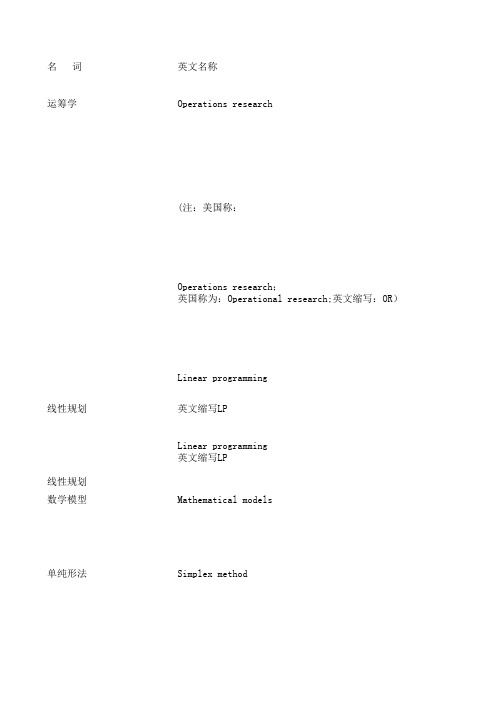
名 词英文名称运筹学Operations research(注:美国称:Operations research;英国称为:Operational research;英文缩写:OR)Linear programming线性规划英文缩写LPLinear programming英文缩写LP线性规划数学模型Mathematical models单纯形法Simplex methodSimplex method单纯形法改进单纯形法Revised Simplex method目标函数Objective约束条件Constraints可行解Feasible solutions可行域Feasible region名 词英文名称线性规划图解法Graphical Solution of Linear Programs对偶理论Duality theory对偶单纯Dual Simplex method形法影子价格Shadow price运输问题transportation problemtransportation problem运输问题目标规划法Goal programming表上作业法Tabular method表上作业法Tabular method图上作业法Graphical method灵敏度分析Sensitivity analysis西北角法Northwest corner rule名 词英文名称最小元素The least cost rule法运输论法Transportation闭回路调整法Close circular adjust method名 词英文名称非线性规划Nonlinear programming斐波那契法Fibonacci search0.618法Golden section search(黄金分割法)欧拉回路Euler loop整数规划Integer programming松弛问题Slack problem名 词英文名称割平面法Cutting plane method分枝限界Branch and bound method法整数线性规划Integer linear programming纯整数线性规划Pure Integer linear programming名 词英文名称混合整数Mixed Integer linear prog.线性规划0-1型整数线性规划Zero-one Integer linear programming 隐枚举法Implicit Enumeration马氏决策Markov decision programming规划最小树问Minimal tree problem题名 词英文名称最短路问Shortest-route problems题Dijkstra算法Dijkstra algorithmFloyd算法Floyd algorithm最大流问Maximal-Flow problems题图与网络分析Graph theory and network analysis 网络计划Network program网络Network网络方法Network method and network planning 和网络计划网络分析Network analysis网络技术Network techniques名 词英文名称关键线路Critical path method 简称CPM法计划评审Program eval-法uation & rev-iew technique简称PERT网络图Network graphic多重图和Multiple graph and简单图simple graph连通图Connected graph无向图Non-oriented graph有向图oriented graph名 词英文名称最短路径问题Shortest path problem动态规划Dynamic programming缩写DP决策Decision决策论Decision theory名 词英文名称现代决策Modern decision theory理论古典决策Classical decision theory理论战略决策Strategy decision风险型决Risk decision策益损矩阵Opportunity loss matrix最大可能Maximal probability criterion法名 词英文名称期望值法Expected value method决策树法Decision trees method局中人Player策略Policy马氏决策Markov decision programming规划英文缩写:MDP悲观准则Max-min criterion(max-min准则)乐观准则Max-max criterion名 词英文名称折衷准则Trade-off criterion等可能准则(Laplace准则)Laplace criterion遗憾准则(min-max准则)Regret criterion对策论Game theory合作对策Cooperative games名 词英文名称非合作对Non-cooperative games 策纳什平衡Nash equilibrium帕雷托最Pareto optimality优斯塔克尔贝格对策Stackelberg strategy统筹法Overall planning method 指派问题Assignment problem匈牙利解Hungarian method法存储论Inventory theory排队论Queuing theory名 词英文名称排队系统Queuing system生灭过程Birth-death process支付矩阵The payoffmatrix内 容运筹学是一门运用于管理有组织系统的科学。
PMP名词翻译及解释
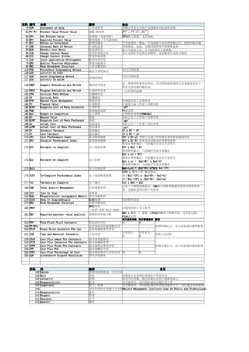
页码缩写49SOW52PV/FV53 53 54 54 55 65 66 78 79 92 116 116 117 117NPVEPVROIIRRBCRCCBCCSJADQFDWBSPDMAONADMAOA全拼Statement of workPresent Value/Future ValueNet Present ValueExpected Present ValueReturn on InvestmentInternal Rate of ReturnBenefit Cost RatioChange Control BoardChange Control SystemJoint Application DevelopmentQuality Function DeploymentWork Breakdown StructurePrecedence Diagramming MethodActivity On NodeArrow Diagramming MethodActivity On ArrowGraphic Evaluation and ReviewProgram Evaluation and ReviewCritical Path MethodCritical PathEarned Value ManagementPlanned ValueBudgeted Cost of Work ScheduledBudget at CompletionEarned ValueBudgeted Cost of Work PerformedActual CostActual Cost of Work PerformedSchedule VarianceCost VarianceCost Performance IndexSchedule Performance IndexEstimate to Complete翻译工作说明书现值/将来值净现值(考虑风险)期望现值(不考虑风险)投资回报率内部收益率收益成本比变更控制委员会变更控制系统联合应用开发质量功能展开工作分解结构紧前关系绘图法箭线绘图法图形评审技术计划评审技术关键路径法关键路径挣值管理计划价值计划价值绩效测量基准完工预算挣值挣值实际成本实际成本进度偏差成本偏差成本绩效指数进度绩效指数完工尚需估算备注对醒目所需交付的产品或服务的叙述性说明PV FV/(1 R)NNPV=收入现值-支出现值不考虑现值,静态;年均利润与项目投资额之比,投资回报率越考虑现值,动态;为收回投资每年的净收益率收入与成本之比,大于1的项目才值得做是正式的但不是固定的组织;是拍板的不是给方案的单代号网络图双代号网络图是一种典型的条件绘图法,采用类似流程图的方法来描述项目中的分支活动或回路活动三点估算的起源119GERT128 133 138 166 168 168 168 168 168 168 169 169 169 170 170 171PERT CPM CP EVM PV BCWS PMB BAC EV BCWP AC ACWP SV CV CPI SPI172ETC 172EAC 173EACt173TCPI174VAC 185TQM188 218 240 278JITRAMKISSRBSEstimate at Complete完工估算完工时间估算To-Complete Performance IndexVariance at CompleteTotal Quality ManagementJust In TimeResponsibility Assignments MatrixKeep It Simple&StupidRisk Breakdown Structure完工尚需绩效指数完工偏差全面质量管理控制成本的工具和技术计划要完成工作量×预算单价"=PV"PV的总和在挣值管理领域PMB=BAC实际已完工工作量×预算单价"=EV"实际已完工工作量×实际单价"=AV"SV = EV - PVCV = EV - AVCPI = EV/AC 考核已完成工作的成本效率即资源利用率SPI = EV/PV 说明项目团队的时间利用效率假设非典型偏差:当前偏差在以后不会发生ETC = BAC - EV假设典型偏差:当前偏差代表未来偏差EAC = AC + ETC假设非典型偏差:当前偏差在以后不会发生EAC = AC + (BAC-EV) = BAC-CV假设典型偏差:当前偏差代表未来偏差EAC = AC + (BAC-EV)/CPI = BAC/CPIEACt = 原计划完工时间/SPITCPI = 剩余工作/剩余资金基于BAC:TCPI = (BAC-EV)/(BAC-AC)基于EAC:TCPI = (BAC-EV)/(EAC-AC)VAC = BAC - EAC由朱兰与费根堡姆提出;TQM和六西格玛既能改进项目的管理质量,也能改进项目的产品质量283SWOT292EMV Expected monetary value analysis 零库存责任分配矩阵KISS原则保持简单浅显风险分解结构SWOT分析识别风险的工具与技术(优势/劣势/机会/威胁)EMV = 概率 × 影响 与P286的概率×影响不同,这里是定量,预期货币价值分析P286是定性买方成本风险买方管理成本适用315FFP Firm Fixed Price Contracts 316FP-EPA315FPIF Fixed Price Incentive Fee Con 321T&M319 318 317 320 320 333CPAFCPIFCPFFCPFCPPCADR固定总价合同低总价加经济价格调整合同总价加激励费用合同买卖双方一Time and Material Contracts工料合同样Cost Plus Award Fee Contracts成本加奖励费用Cost Plus Incentive Fee Contracts成本加激励费用Cost Plus Fixed Fee Contracts成本加固定费用合同Cost Plus Fee成本加酬金合同Cost Plus Percentage of Cost成本加按成本百分比合同高Alternative Dispute Resolution替代争议解决低范围明确定义,买方有很强的谈判优势买卖双方一有较大灵活性样范围有限定义,卖方有很强的谈判优势高页码189219219219219346348348348348词KaizenRoleAuthorityResponsibilityCompetencyResponsibilityRespectFairnessHonesty备注翻译持续改进的意思,日本名词说明某人负责项目某部分工作的名词角色使用项目资源、做出决策以及签字批准的权力职权为完成项目,项目团队成员应履行的工作职责为完成项目,项目团队成员所需的技能和才干,可以通过培训获得能力、资格Project Management Institute Code of Ethics and Professional项目管理协会道德与专业行为责任尊重公平诚实。
UnconstrainedPaths解决办法

UnconstrainedPaths解决办法⽤TimeQuest对DAC7512控制器进⾏时序分析在对某个对象下时序约束的时候,⾸先要能正确识别它,TimeQuest 会对设计中各组成部分根据属性进⾏归类,我们在下时序约束的时候,可以通过命令查找对应类别的某个对象。
TimeQuest对设计中各组成部分的归类主要有cells,pins,nets和ports ⼏种。
寄存器,门电路等为cells;设计的输⼊输出端⼝为ports;寄存器,门电路等的输⼊输出引脚为pins;ports和pins之间的连线为nets。
具体可以参照下图(此图出⾃Altera Time Quest的使⽤说明)。
下⾯我们按照本⽂第⼆部分⽤TimeQuest做时序分析的基本操作流程所描述的流程对DAC7512控制器进⾏时序分析。
建⽴和预编译项⽬的部分相对简单,涉及到的也只是QuartusII的⼀些基本操作,这⾥我们就不再做具体的叙述。
主要介绍如何向项⽬中添加时序约束和如何进⾏时序验证。
⾸先建⽴⼀个名称与项⽬top层名字⼀致的sdc⽂件,然后按照下⾯的步骤添加时序约束。
1. 创建时钟添加时序约束的第⼀步就是创建时钟。
为了确保STA结果的准确性,必须定义设计中所有的时钟,并指定时钟所有相关参数。
TimeQuest⽀持下⾯的时钟类型:a) 基准时钟(Base clocks)b) 虚拟时钟(Virtual clocks)c) 多频率时钟(Multifrequency clocks)d) ⽣成时钟(Generated clocks)我们在添加时序约束的时候,⾸先创建时钟的原因是后⾯其它的时序约束都要参考相关的时钟的。
基准时钟:基准时钟是输⼊到FPGA中的原始输⼊时钟。
与PLLs输出的时钟不同,基准时钟⼀般是由⽚外晶振产⽣的。
定义基准时钟的原因是其他⽣成时钟和时序约束通常都以基准时钟为参照。
很明显,在DAC7512控制器中,CLK_IN是基准时钟。
JMP中文教程doe试验设计_1

Copyright © 2008, SAS Institute Inc. All rights reserved.
如何鉴定流程能力的优劣?
Target LSL USL
Copyright © 2008, SAS Institute Inc. All rights reserved.
质量管理的发展
传统控制 阶段 (QC, quality control) 统计质量 控制阶段 (SQC, statistical quality control)
全球最优秀的行业领袖信赖JMP
Copyright © 2008, SAS Institute Inc. All rights reserved.
JMP ——让质量改进更轻松
易学易用 全面而强大的分析能力 卓越的可视化及项目推广能力
Copyright © 2008, SAS Institute Inc. All rights reserved.
交互作用
No Interaction
–1 Factor B Y +1 Y –1 +1 Factor B
Interaction
–1
+1
–1
+1
Factor A
Factor A
Effect of A at B(+) Interaction
=
–
2
Effect of A at B(-)
Copyright © 2008, SAS Institute Inc. All rights reserved.
Seeing is believing!
Copyright © 2008, SAS Institute Inc. All rights reserved.
Critical path method关键路线法

Critical path method 关键路线法关键路线法(Critical Path Method,CPM)是一种通过分析哪个活动序列(哪条路线)进度安排的灵活性(总时差)最少来预测项目工期的网络分析技术。
具体而言,该方法依赖于项目网络图和活动持续时间估计,通过正推法计算活动的最早时间,通过逆推法计算活动的最迟时间,在此基础上确定关键路线,并对关键路线进行调整和优化,从而使项目工期最短,使项目进度计划最优。
关键路线法的关键是确定项目网络图的关键路线,这一工作需要依赖于活动清单、项目网络图及活动持续时间估计等,如果这些文档已具备,借助于项目管理软件,关键路线的计算可以自动完成,如果采用手工计算,可以遵循以下步骤:(1)把所有的项目活动及活动的持续时间估计反映到一张工作表中,如表5-3所示。
(2)计算每项活动的最早开始时间和最早结束时间,计算公式为EF=ES+活动持续时间估计。
(3)计算每项活动的最迟结束时间和最迟开始时间,计算公式为LS=LF-活动持续时间估计。
(4)计算每项活动的总时差,计算公式为TF=LS-ES=LF-EF。
(5)找出总时差最小的活动,这些活动就构成关键路线。
尽管关键路线法与关键路线不同,但在了解关键路线法之前了解关键路线的含义还是非常必要的,关键路线的概念在上面已提及。
对于一个项目而言,只有项目网络图中的最长的或耗时最多的活动路线完成之后,项目才能结束,这条最长的活动路线就叫做关键路线(Critical Path)。
根据关键路线的含义,关键路线具有以下特点:A、关键路线上的活动的持续时间决定项目的工期,关键路线上所有活动的持续时间加起来就是项目的工期。
B、关键路线上的任何一个活动都是关键活动,其中任何一个活动的延迟都会导致整个项目完成时间的延迟。
C、关键路线是从始点到终点的项目路线中耗时最长的路线,因此要想缩短项目的工期,必须在关键路线上想办法,反之,若关键路线耗时延长,则整个项目的完工期就会延长。
项目进度控制方法

项目进度控制方法项目管理中,控制项目进度是确保项目按计划进行的重要环节。
项目进度控制方法的目标是提高项目进度的可控性,以便实现项目的及时投入使用和交付。
本文将介绍几种常用的项目进度控制方法。
一、关键路径法(Critical Path Method,简称CPM)关键路径法是一种基于网络图的项目进度控制方法,通过分析项目中各个活动的前置关系和持续时间,找出影响项目整体进度的关键路径,从而实现对项目进度的控制。
关键路径法的重点在于确定项目中的关键活动和关键路径,以便正确调配资源,避免资源的闲置和浪费。
关键路径法的步骤包括创建网络图、计算各个活动的最早开始时间、最晚开始时间和总时差,确定关键活动和关键路径,制定合理的进度计划,以及及时调整进度计划以应对变化。
二、里程碑法(Milestone Method)里程碑法是将项目进度划分为若干里程碑,每个里程碑代表项目完成的重要阶段或节点。
通过设定里程碑,可以及时评估项目的进展情况,并依此对项目进度进行控制。
里程碑法的关键在于准确设定里程碑并制定清晰的里程碑完成标准。
在项目执行过程中,每当达到一个里程碑,就进行评估和控制,及时发现问题并采取相应措施,以确保项目按时进行。
三、进度差异分析法(Schedule Variance Analysis)进度差异分析法通过比较实际进度和计划进度的差异来评估项目的进展情况。
这种方法以进度偏差为基础,通过计算偏差率和偏差幅度,检查项目是否存在计划延迟或提前。
进度差异分析法提供了一种直观的方式来评估项目的进度控制情况。
如果项目进度滞后于计划,就可以及时采取纠正措施。
此外,通过频繁的进度差异分析,可以建立起对项目进度的持续监控和调整机制,确保项目按计划进行。
四、资源平衡法(Resource Leveling)资源平衡法是一种通过优化资源的分配和利用来实现项目进度控制的方法。
在项目执行过程中,可能会出现资源供需不平衡的情况,导致项目进度延迟。
关键路径法(CriticalPathMethod,CPM)
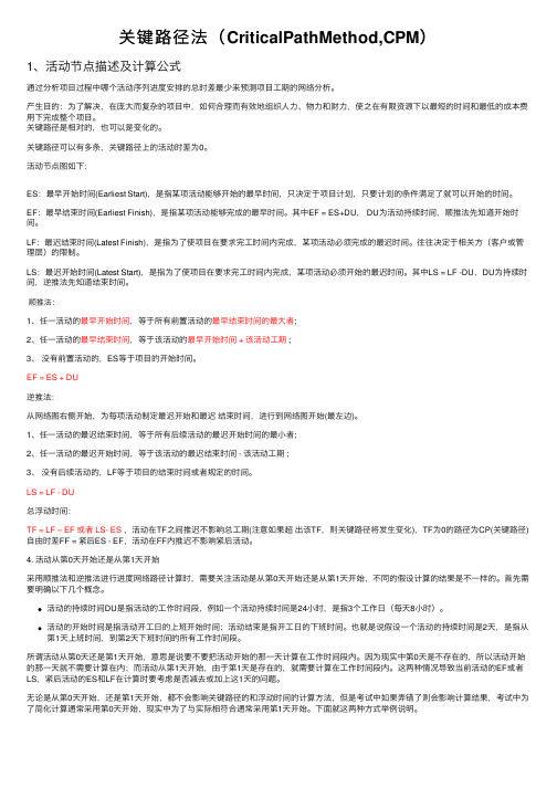
关键路径法(CriticalPathMethod,CPM)1、活动节点描述及计算公式通过分析项⽬过程中哪个活动序列进度安排的总时差最少来预测项⽬⼯期的⽹络分析。
产⽣⽬的:为了解决,在庞⼤⽽复杂的项⽬中,如何合理⽽有效地组织⼈⼒、物⼒和财⼒,使之在有限资源下以最短的时间和最低的成本费⽤下完成整个项⽬。
关键路径是相对的,也可以是变化的。
关键路径可以有多条,关键路径上的活动时差为0。
活动节点图如下:ES:最早开始时间(Earliest Start),是指某项活动能够开始的最早时间,只决定于项⽬计划,只要计划的条件满⾜了就可以开始的时间。
EF:最早结束时间(Earliest Finish),是指某项活动能够完成的最早时间。
其中EF = ES+DU, DU为活动持续时间,顺推法先知道开始时间。
LF:最迟结束时间(Latest Finish),是指为了使项⽬在要求完⼯时间内完成,某项活动必须完成的最迟时间。
往往决定于相关⽅(客户或管理层)的限制。
LS:最迟开始时间(Latest Start),是指为了使项⽬在要求完⼯时间内完成,某项活动必须开始的最迟时间。
其中LS = LF -DU,DU为持续时间,逆推法先知道结束时间。
顺推法:1、任⼀活动的最早开始时间,等于所有前置活动的最早结束时间的最⼤者;2、任⼀活动的最早结束时间,等于该活动的最早开始时间 + 该活动⼯期 ;3、没有前置活动的,ES等于项⽬的开始时间。
EF = ES + DU逆推法:从⽹络图右侧开始,为每项活动制定最迟开始和最迟结束时间,进⾏到⽹络图开始(最左边)。
1、任⼀活动的最迟结束时间,等于所有后续活动的最迟开始时间的最⼩者;2、任⼀活动的最迟开始时间,等于该活动的最迟结束时间 - 该活动⼯期 ;3、没有后续活动的,LF等于项⽬的结束时间或者规定的时间。
LS = LF - DU总浮动时间:TF = LF – EF 或者 LS- ES,活动在TF之间推迟不影响总⼯期(注意如果超出该TF,则关键路径将发⽣变化),TF为0的路径为CP(关键路径)⾃由时差FF = 紧后ES - EF,活动在FF内推迟不影响紧后活动。
(项目管理)项目专业术语
项目范围管理基准计划(baseline)概念开发(conceptual development)配置管理(configuration management)控制系统(control system)成本控制账户(cost control accounts)成本加成合同(cost-plus contracts)可交付成果(deliverable)里程碑(milestone)组织分解结构(organization breakdown structure, OBS)项目收尾(project closeout)项目范围(project scope)责任分配矩阵(responsibility assignment matrix, RAM)范围基准计划(scope baseline)范围蔓延(scope creep)范围管理(scope management)范围报告(scope reporting)范围说明(scope statement)工作说明书(statement of work, SOW)总承包合同(turnkey contracts)工作分解结构代号(WBS codes)工作授权(work authorization)工作分解结构(work breakdown structure, WBS)工作包(work package)项目风险管理可能性和后果分析(analysis of probability and consequences)变更管理(change management)商业风险(commercial risk)应急储备金(contingency reserves)合约/法律风险(contractual/legal risk)控制和文档化(control and documentation)交叉培训(cross-training)执行风险(execution risk)财务风险(financial risk)固定总价合同(fixed-price contract)违约赔偿金(liquidated damage)管理应急金(managerial contingency)指导(mentoring)项目风险(project risk)项目风险分析和管理(project risk analysis and management, PRAM) 风险识别(risk identification)风险管理(risk management)风险缓解策略(risk mitigation strategies)任务应急金(task contingency)技术风险(technical risk)项目团队的建设、冲突和谈判可接近性(accessibility)中止(adjourning)管理上的冲突(administrative conflict)凝聚力(cohesiveness)冲突(conflict)跨职能合作(cross-functional cooperation) 差异化(differentiation)成立阶段(forming stage)挫败(frustration)基于目标的冲突(goal-oriented conflict)互动(interaction)相互依赖(interdependencies)个人之间的冲突(interpersonal conflict)谈判(negotiation)规范化阶段(norming stage)目标(orientation)结果(outcome)实施阶段(performing stage)物理位置上的接近(physical proximity)原则性谈判(principled negotiation)社会心理结果(psychosocial outcomes)中断平衡(punctuated equilibrium)冲突风暴(storming)最高目标(superordinate goals)任务结果(task outcomes)团队建设(team building)信任(trust)虚拟团队(virtual teams)成本估算和预算基于活动的估算(ABC, activity-based costing)自下而上的预算(bottom-up budgeting)应急费用预算(budget contingency)成本估算(cost estimation)赶工(crashing)最终估算(definitive estimates)直接成本(direct costs)加速成本(expedited costs)可行性估算(feasibility estimates)固定成本(fixed costs)间接成本(indirect costs)学习曲线(learning curve)一次性成本(nonrecurring costs)正常成本(normal costs)参数估算(parametric estimation)项目预算(project budget)经常性成本(recurring costs)分阶段预算(time-phased budget)自上而下的预算(top-down budgeting)变动成本(variable costs)项目进度计划:网络、历时估计和关键路径活动,也称任务(activity, or task)双代号网络图法(activity-on-arrow)单代号网络图法(activity-on-node)箭线(Arrow)逆推法(backward pass)β分布(beta distribution)发散活动(burst activity)并行活动(concurrent activities)置信区间(confidence interval)赶工(crashing)关键路径(critical path)关键路径法critical path method ()历时估计(duration estimation)最早开始时间(early start date, ES)事件(event)浮动时差(float, or slack)正推法(forward pass)集合活动(hammock activities)阶梯化活动(laddering activities)最晚开始时间(late start date)汇聚活动(merge activities)网络图(network diagram)节点(node)排好序的活动(ordered activities)路径(path)前置活动(predecessors)计划评审技术(program evaluation and review technique) 项目网络图(project network diagram, PND)项目计划编制(project planning)有限资源进度计划(resource-limited schedule)范围(scope)串行活动(serial activities)后续活动(successors)任务(task)工作分解结构(work breakdown structure)工作包(work package)项目进度计划:滞后、赶工和活动网络活动(也称任务)(activity,也称task)双代号网络图(activity-on-arrow, AOA)单代号网络图(activity-on-node, AON)箭线(Arrow)逆推法(backward pass)赶工(crashing)关键路径(critical path)虚活动(dummy activities)最早开始时间(early start date, ES)事件(event)浮动时差(float, or slack)正推法(forward pass)甘特图(Gantt chart)滞后(lag)最晚开始时间(late start date)汇聚(merge)节点(node)计划评审技术(Program Evaluation and Review Technique, PERT)串行活动(serial activities)后续活动(successors)任务(task,见activity)关键链项目进度计划能力约束缓冲(capacity constraint buffer, CCB)中心极限理论(central limits theorem)普通原因偏差(common cause variation)关键链(critical chain)关键链项目管理(critical chain project management, CCPM)鼓点(drum)鼓点缓冲(drum buffers)多任务处理(multitasking)消极偏差(negative variation)积极偏差(positive variation)特殊原因偏差(special cause variation)学生综合症(student syndrome)约束理论(theory of constraints, TOC)资源管理平衡试探法(leveling heuristics)混合约束型项目(mixed-constraint project)物质约束(physical constraints)资源约束型项目(resource- constrained project)资源约束(resource constraints)资源平衡(resource leveling)资源负载(resource loading)资源负载图(resource-loading charts)资源负载表(resource-loading table)平滑(smoothing)分割活动(splitting activities)时间约束型项目(time-constrained project)项目评估和控制已完成工作实际成本(actual cost of work performed, AC)完工预算(budgeted cost at completion, BAC)控制循环(control cycle)成本绩效指数(cost performance index, CPI)挣值(earned value, EV)挣值管理(earned value management, EVM)里程碑(milestone)计划值(planned value, PV)项目基准计划(project baseline)项目控制(project control)项目S曲线(project S-curve)进度绩效指数(schedule performance index, SPI)进度偏差(schedule variance)跟踪甘特图(tracking Gantt charts)项目收尾和中止仲裁(arbitration)建造-经营-转让(build, operate, transfer, BOT)建造-拥有-经营-转让(build, own, operate, transfer, BOOT)默认索赔(default claims)争议(disputes)提前终止(early termination)特惠索赔(ex-gratia claims)经验教训(lessons learned)自然终止(natural termination)私人主动融资(private finance initiatives, PFIs)项目终止(project termination)附加式终止(termination by addition)绝对式终止(termination by extinction)集成式终止(termination by integration)自灭式终止(termination by starvation)非自然终止(unnatural termination)。
Critical Path Method

CVEN90045 Engineering Project Implementation
Planning and Scheduling
A B C D E F G Manufacture tank stand (3 days) Construct foundations (2 days) Install tank stand (2 days) Excavate trench for water mains (1 day) Install tank (1 day) Lay water mains (1 day) Delivery pumps (7 days)
CVEN90045 Engineering Project Implementation
Planning & Scheduling
CVEN90045 Engineering Project Implementation
WHERE, WHEN AND WHO
CVEN90045 Engineering Project Implementation
A process of quantifying the program (e.g. determining times and costs of activities, and the efficiency of allocated resources)
CVEN90045 Engineering Project Implementation
CVEN90045 Engineering Project Implementation
Concept of Planning
• Definition of Planning Terms
Planning Programming
工程投标规划书中的工期控制与进度管理方法
工程投标规划书中的工期控制与进度管理方法工期控制与进度管理是项目管理中一个至关重要的环节,尤其在工程投标规划书中更是必不可少的一部分。
本文将介绍几种常用的工期控制与进度管理方法,以供工程投标规划书的编写参考。
一、关键路径法(Critical Path Method,简称CPM)关键路径法是一种常用的工期控制与进度管理方法,它可以帮助项目团队确定整个项目的关键路径,并制定相应的措施以保证工期控制。
关键路径法的核心是通过网络计划图的绘制和计算,找出项目中工序之间的依赖关系和耗时,从而确定关键路径。
在编写工程投标规划书时,可以使用关键路径法详细列出项目中每个工序的时间和关键路径,以便投标人能够清晰地了解工期控制的重要性和可行性。
二、里程碑法(Milestone Method)里程碑法是一种以达到关键节点为目标的工期控制与进度管理方法。
里程碑是指项目中的重要节点,通常是一些关键工序的完成时间点。
在工程投标规划书中,我们可以根据项目的具体情况,设定一些重要的里程碑,并制定相应的措施以确保在规定时间内达到这些里程碑。
里程碑法在工期控制中具有较好的可操作性和可控性,能够有效地管理项目的进度。
三、资源平衡法(Resource Leveling Method)资源平衡法是一种基于资源需求的工期控制与进度管理方法。
在编写工程投标规划书时,我们需要对项目的资源进行充分的考虑,包括人力、物力、财力等方面的资源需求。
资源平衡法通过合理调配资源,尽量平衡项目中不同工序之间的资源需求,从而达到工期控制和进度管理的目标。
在写作工程投标规划书时,我们可以详细说明项目中各个工序所需资源的分配和调配情况,以便投标人了解工期控制与进度管理的策略和方法。
四、进度把控法(Schedule Control Method)进度把控法是一种针对项目进度的监控和控制手段,在工程投标规划书中具有重要作用。
进度把控法通过设定工序的开始时间和完成时间,并监控实际的进度情况,及时调整和控制进度,确保项目按时完成。
建构的四种方法序列
建构的四种方法序列English:The four methods of construction sequencing are critical to the successful execution of any project. The first method is known as the critical path method (CPM), which involves identifying the longest path of dependent activities that determine the overall duration of the project. The second method is the program evaluation and review technique (PERT), which is similar to the CPM but takes into account uncertainties and variations in activity duration. The third method is called the Gantt chart, which is a visual representation of the project schedule that allows for the tracking of progress and dependencies between activities. The fourth method is the line of balance (LOB) method, which is commonly used in repetitive construction projects and focuses on the efficient allocation of resources and labor over time.中文翻译:建构序列的四种方法对于成功执行任何项目至关重要。
项目管理中的时间进度管理课件培训课件(PPT 127张)

控制其执行,必要时调整进度计划 审核项目各参与方(如设计方、施工方和材料设备供货方)
提出的进度计划/供货计划,检查、督促和控制其执行 在项目实施过程中,每月进行计划值与实际值的比较,
每月、季、年度提交各种进度控制报告和报表
14
项目进度计划的表现形式
依据:以工作分解结构图表和项目组织结构图表为依据制作此表。
安加排强后 控续制支点持的服复务测以工及作保动,护为态客户控提供制相应原的技理术支为持服指务;导进行进度计划值与实际值的比
较 费用
进度
项目进度计划的表现形式
关键线路法CPM(critical path method)
可采取组织、技术、经济、合同措施 网络图中箭线端部的圆圈或其它形式的封闭图形。
9
一个进度管理的经典例证
A: 一般工作顺序---流水作业 B: 改变工作顺序(逻辑)会影响项目总时间(工
期)。某些工作决定了项目总工期,而某些 (在一定范围内)不会 C: 改变工作持续时间会影响项目总工期 D:经过优化(工作顺序和持续时间),可供实 施
10
进度计划的数学分析方法
关键线路法CPM(critical path method) 计划评审技术PERT(program evaluation
2、对可能发生变化的地方给以特别的关注
有必要进行计算机辅助进度控制 完成本工作的协作单位和部门
工作活动清单必须包括本项目范围内的所有工作,应当对每项工作作出文字说明,保证项目成员准确完整地理解该项工作。
进度控制的协调工作量大
13
进度控制的主要工作内容
项目建设周期总进度目标的分析、论证 编制项目总进度规划,在项目实施过程中控制其执行,
critical path analysis practice

critical path analysis practice Critical Path Analysis (CPA) is a project management technique used to identify the most critical tasks and sequence of activities that determine the total duration of a project. Here are some practice steps for Critical Path Analysis:1. Identify Tasks:• List all the tasks involved in the project.• Define the dependencies between tasks, i.e., which tasks must be completed before others can start.2. Estimate Durations:• Estimate the time required to complete each task.• Use historical data, expert opinions, or other relevant information to make realistic estimates.3. Create a Network Diagram:• Use the identified tasks and dependencies to create a network diagram. This is often done using a PERT (Program Evaluation and Review Technique) chart or a Gantt chart.• Nodes in the diagram represent tasks, and arrows represent dependencies.4. Determine Early Start (ES) and Early Finish (EF):• Calculate the earliest start time (ES) for each task. The ES for the first task is 0.• Calculate the earliest finish time (EF) for each task using the formula: EF = ES + Duration.5. Determine Late Start (LS) and Late Finish (LF):• Calculate the latest finish time (LF) for the last task in the project. LF for the last task is equal to its EF.• Calculate the latest start time (LS) for each task using the formula: LS = LF - Duration.6. Calculate Slack (Float):• Slack is the amount of time a task can be delayed without affecting the project's completion time.• Slack = LS - ES or LF - EF for each task.7. Identify the Critical Path:• Tasks with zero slack are on the critical path.• The critical path is the longest path through the network diagram and represents the minimum project duration.8. Monitoring and Controlling:• Regularly update the project schedule as tasks are completed or delayed.• Monitor critical tasks to ensure the project stays on schedule.9. Risk Analysis:• Consider uncertainties and risks associated with task durations.• Perform a sensitivity analysis to identify tasks with the most significant impact on project completion.10. Resource Allocation:• Consider resource constraints and allocate resources effectively to optimize the project schedule.Practicing Critical Path Analysis involves working through these steps with a specific project. Using project management software can simplify the process and help visualize the critical path and project schedule.。
[项目管理]CPM关键路径法(CriticalPathMethod)
![[项目管理]CPM关键路径法(CriticalPathMethod)](https://img.taocdn.com/s3/m/bcd597ec0342a8956bec0975f46527d3250ca65f.png)
CPM关键路径法(Critical Path Method)关键路径法起源关键路线法是一种网络图方法,由雷明顿-兰德公司(Remington- Rand)的JE克里(JE Kelly)和杜邦公司的MR沃尔克(MR Walker)在1957年提出的,用于对化工工厂的维护项目进行日程安排。
它适用于有很多作业而且必须按时完成的项目。
关键路线法是一个动态系统,它会随着项目的进展不断更新,该方法采用单一时间估计法,其中时间被视为一定的或确定的。
利用关键路线法的步骤1)画出网络图,以节点标明事件,由箭头代表作业。
这样可以对整个项目有一个整体概观。
习惯上项目开始于左方终止于右方。
2)在箭头上标出每项作业的持续时间(T)3)从左面开始,计算每项作业的最早结束时间(EF)。
该时间等于最早可能的开始时间(ES)加上该作业的持续时间。
4)当所有的计算都完成时,最后算出的时间就是完成整个项目所需要的时间。
5)从右边开始,根据整个项目的持续时间决定每项作业的最迟结束时间(LF)。
6)最迟结束时间减去作业的持续时间得到最迟开始时间(LS)。
7)每项作业的最迟结束时间与最早结束时间,或者最迟开始时间与最早开始时间的差额就是该作业的时差。
8)如果某作业的时差为零,那么该作业就在关键路线上。
9)项目的关联路线就是所有作业的时差为零的路线。
CPM在项目管理中的应用对于一个项目而言,只有项目网络中最长的或耗时最多的活动完成之后,项目才能结束,这条最长的活动路线就叫关键路径(Critical Path),组成关键路径的活动称为关键活动。
其通常做法是:1)将项目中的各项活动视为有一个时间属性的结点,从项目起点到终点进行排列;2)用有方向的线段标出各结点的紧前活动和紧后活动的关系,使之成为一个有方向的网络图;3)用正推法和逆推法计算出各个活动的最早开始时间,最晚开始时间,最早完工时间和最迟完工时间,并计算出各个活动的时差;4)找出所有时差为零或者为负数的活动所组成的路线,即为关键路径;5)识别出准关键路径,为网络优化提供约束条件;它具有以下特点:1)关键路径上的活动持续时间决定了项目的工期,关键路径上所有活动的持续时间总和就是项目的工期。
critical path method和metra potential method的区别
Critical Path Method 和 Metra Potential Method 的区别在项目管理中,关键路径法(Critical Path Method,简称 CPM)和代谢潜力法(Metra Potential Method,简称 MPM)是两种常用的进度计划方法。
它们都可以用来确定项目的最短完成时间,但它们的计算方法和应用场景有所不同。
本文将对这两种方法进行比较,以帮助读者更好地理解它们的区别和应用。
下面是本店铺为大家精心编写的3篇《Critical Path Method 和 Metra Potential Method 的区别》,供大家借鉴与参考,希望对大家有所帮助。
《Critical Path Method 和 Metra Potential Method 的区别》篇11. 计算方法关键路径法(CPM)是一种基于网络图的计算方法,它通过计算每个活动的最早开始时间(EST)、最晚开始时间(LST)、最早完成时间(EFT)和最晚完成时间(LFT)来确定项目的关键路径。
在 CPM 中,关键路径是指连接起始节点和结束节点的路径中,总耗时最长的路径。
CPM 通常采用逆推法,从项目的结束时间开始,逐步推算出每个活动的最早和最晚开始时间,从而确定项目的进度计划。
代谢潜力法(MPM)是一种基于活动历时的计算方法,它通过计算每个活动的最早开始时间(EST)、最晚开始时间(LST)、最早完成时间(EFT)和最晚完成时间(LFT)来确定项目的进度计划。
在 MPM 中,代谢潜力是指项目中最短完成时间与实际完成时间之间的差值,它反映了项目进度的弹性。
MPM 通常采用正推法,从项目的开始时间开始,逐步推算出每个活动的最早和最晚完成时间,从而确定项目的进度计划。
2. 应用场景关键路径法(CPM)适用于那些具有固定截止日期的项目,它的计算结果可以帮助项目经理确定项目的最短完成时间,以及关键路径上的活动。
CPM 的缺点是它假定所有活动的历时是固定的,因此无法考虑活动的灵活性和可变性。
会展项目进度计划关键路径法

会展项目进度计划关键路径法The Critical Path Method (CPM) is a crucial tool in project management, particularly in the context of exhibition planning. It involves the identification of the longest path through a project's network diagram, representing the sequence of tasks that determines the overall duration of the project. The CPM helps in effectively allocating resources, predicting project completion dates, and managing potential delays.关键路径法(CPM)是项目管理中的一个重要工具,特别是在会展规划方面。
它涉及识别项目网络图中的最长路径,该路径代表决定项目整体持续时间的任务序列。
CPM有助于有效分配资源、预测项目完成日期以及管理潜在的延误。
In the context of exhibition project scheduling, CPM is employed to identify the critical path, which comprises the tasks that have no float time—in other words, they must be completed on time to ensure the overall project deadline is met. This method allows project managers to prioritize tasks, allocate resources efficiently, and monitor progress closely.在会展项目进度规划的背景下,关键路径法用于确定关键路径,该路径由没有浮动时间的任务组成——换句话说,这些任务必须按时完成,以确保整个项目能在截止日期前完成。
- 1、下载文档前请自行甄别文档内容的完整性,平台不提供额外的编辑、内容补充、找答案等附加服务。
- 2、"仅部分预览"的文档,不可在线预览部分如存在完整性等问题,可反馈申请退款(可完整预览的文档不适用该条件!)。
- 3、如文档侵犯您的权益,请联系客服反馈,我们会尽快为您处理(人工客服工作时间:9:00-18:30)。
UDepartment of Critical Path Method Applied AgricultureForest Service to Research Project Planning: Pacific SouthwestForest and Range Fire Economics Evaluation Experiment StationGeneral Technical System (FEES)Report PSW-93The Authors:EARL B. ANDERSON is a supervisory physical scientist and leader of the Site-Specific Fire Prescriptions for California Chaparral and Associated Ecosystems research project headquartered at Riverside, California. At the time this work was accomplished, he was an operations research analyst in the Station's Fire Management Planning and Economics project. He earned a degree (1951) in mechanical engineering at the University of Illinois. He was a member of the technical staff of Aerospace Corporation, El Segundo, California, from 1962 until he joined the Station's staff in 1978. R. STANTON HALES is the associate dean and professor of mathematics, Pomona College, California. He holds degrees in mathematics from Pomona College (bachelor's 1964) and from Harvard University (master's 1965, doctorate 1970).Acknowledgments:We thank the many students and faculty members of the Claremont Colleges who contributed to this work. In particular, a large share of credit for development of the planning system described belongs to a team in the Claremont Graduate School Mathe-matics Clinic under the leadership of Suzanne Larson. The team included Carl Ito, David Nicastro, and Michael O'Keeffe--all students at Pomona College--and was assisted by professors Irwin Schochetman, Oakland University, while visiting the Claremont Gradu-ate School, and Terence R. Shore, California State University, Dominguez Hills, while visiting Pomona College.Publisher:Pacific Southwest Forest and Range Experiment Station PO. Box 245, Berkeley, California 94701August 1986Critical Path Method Appliedto Research Project Planning: Fire Economics Evaluation System (FEES)Earl B. Anderson R. Stanton HalesCONTENTSIntroduction (1)Critical Path Method (CPM) (1)Constructing a Network Diagram (2)Calculating Start and Finish Times (3)Constructing a Time Chart (4)Methods of Schedule Selection (5)Resource Analysis (5)Cost Analysis (6)Fire Economics Evaluation System (6)Comparing Schedules (7)Updating the Routine (8)References (8)iINTRODUCTIONN etwork techniques are often used in scheduling projects that contain many interrelated activities. One approach that has been widely used is the critical path method, in which a network diagram depicts precedence among activities. This method also calculates their starting, float, and finishing times to identify critical activities, and it constructs a time chart to display possible project schedules.Typically, network techniques have been used in large and complex projects consisting of thousands of activities, such as major construction and engineering projects. In the 1950's, a critical path technique called PERT (program evaluation and review technique) was developed by the U.S. Navy for manag-ing the Fleet Ballistic Missile (Polaris) submarine project. CPM (critical path method) was developed by the DuPont Company and Remington Rand Univac for managing plant maintenance and construction work.1 Differing--for the most part-only in the level of importance that probabilistic concepts have in their use, these mathematical optimization techniques are referred to collectively as PERT-CPM or simply CPM.Despite the success of PERT-CPM in hardware-oriented programs, its application in resource management problems was initially limited (Davis 1968). But as CPM techniques were modified and designed to operate on the smaller new computer systems, they proved useful in smaller projects such as design and marketing of new products, maintenance and shutdown schedules, and research and development pro-grams. Its potential was apparent for scheduling and monitor-ing development of the Fire Economics Evaluation System (FEES). This simulation model is being developed by the Forest Service's Pacific Southwest Forest and Range Exper-iment Station to relate alternative fire management activities to changes in fire management program costs and resource net values (Mills and Bratten 1982).A survey of more than 30 available computerized CPM systems from more than 20 software suppliers showed that most routines had specific applications and were adapted to specific computer languages and hardware. None were ideally suited nor could be reasonably modified to meet the needs of1Commercial enterprises are mentioned only for information. No endorse-ment by the U.S. Department of Agriculture is implied. developing the FEES project. Therefore, a computerized CPM package was developed under a cooperative agreement with the Mathematics Clinic of the Claremont Colleges, Claremont, California.Since the FEES package was developed, software routines have been created elsewhere and are available for application to other small projects. Therefore, before selecting or develop-ing a CPM system, software operable on the potential users' hardware should be thoroughly searched.This report describes the critical path method, explains the mathematical concepts behind it, and--using the FEES proj-ect as an example--illustrates how a computerized CPM approach can be applied to a resource management or other research project.CRITICAL PATH METHOD (CPM) Translating a project's needs into a mathematical system requires an understanding of general stages within which the CPM routines may be applied: planning, scheduling, and controlling (more appropriately termed "monitoring" for research application).The greatest advantage of CPM is seen at the planning stage. Here the user is required to think through a project logically and with sufficient detail to establish firm, clear project objectives, activities, and specifications. This mini-mizes the chance of overlooking necessary activities and goals of a project.In the scheduling stage, CPM provides a realistic and disciplined method for determining how to attain the project objectives and for communicating and documenting the proj-ect plans clearly and concisely. A time chart is constructed to show the start and finish times for each activity, and the amount of leeway or "float" corresponding to each activity's relationship to other activities in the project.The monitoring stage helps to focus management's atten-tion where it is most needed: on the activities that most constrain the schedule. As activities are completed ahead of or behind schedule, CPM will generate new schedules which allow for those activities, and as technical or procedural changes are considered, CPM will indicate the effect these changes would have on the overall schedule.In the planning and scheduling phases of CPM analysis, three basic steps are carried out:11. Constructing a network diagram to depict precedence among activities2. Calculating start, finish, and slack or float times3. Constructing a time chart to display results of steps 1and 2.Constructing a Network DiagramThe first step in CPM analysis is constructing a network, or arrow, diagram that graphically shows the precedence rela-tionships among project activities, i.e., the order in which activities are to be carried out. An arrow represents an activ-ity; arrowheads indicate the order of those activities. A "node" or point denotes the beginning and end of an activity. Each node then is labeled and represents an event, defined tobe the completion of all activities leading into that node. In general, integers represent nodes and capital letters represent activities.A network diagram can be constructed given the following information: a list of all activities involved in a project and,for each activity, a list of its precedences, i.e., the other activities that must be completed (immediately) before begin-ning that particular activity. For example, the network dia-gram in figure 1 was constructed from the following sample information (duration is expressed in time units, such as weeks or months, appropriate for a specific project):Activity Precedences DurationA - 2B - 2C - 1D A 4E B 5F E 4G B 8H C 3I D 1J I,F 3K G,H 5 2 Four basic rules guide construction of a network diagram(Taha 1971):Rule 1--Each activity is represented by one arrow in the network.Rule 2--"Dummy'' activities are created whenever needed to portray the logic of the relationship between activities. A dummy activity is depicted as a dotted arrow and represents an activity which takes no time and uses no resources. It is needed when a logical relationship between activities cannot otherwise be represented correctly. For example, suppose that in a certain project both activities C and D must precede activity F, and only activity C must precede H:Activity PrecedencesF C,DH CTo represent this situation correctly, one must make use of a dummy activity. The incorrect and correct representations of a dummy activity are shown in fig. 2.Rule 3--No two activities should be identified by the same beginning event and by the same end event.Rule 4--The following questions must be answered as each activity is added to the network, to insure the network correctness:• What activities must be completed immediately before this activity can start?• What activities must follow this activity?Using these four rules, one can create by hand or by computer the network diagram associated with a project. However, many CPM computer routines do not explicitly create the network diagram. Instead, they store activity dura-tion times as a (vector) list of numbers, and immediate prece-dences as a Boolean matrix (tables of 0's and l's) and deal with them algebraically. They are thus able to use the infor-mation that a network diagram provides without actually plotting it, and thus only make implicit use of the diagram. Calculating Start and Finish Times The second step in CPM analysis is calculating start and finish times for activities. Times are calculated using the precedence relationships shown in the network diagram and their durations. Start and finish times are used to determine float times associated with each activity. Float times are used to identify critical activities.The calculations involve two phases: the "forward pass" and the "backward pass." The forward pass involves a sequence of calculations beginning at the start of the network and moving forward toward the end of the network. This phase computes the earliest possible finish time. The back-ward pass involves a sequence of calculations beginning at the end of the network and moving backward toward the start of the network. This phase computes the latest possible finish time.Each activity of the network diagram (fig. 1) can be denoted either by its end nodes (i, j) or activity name (I). Let the earliest time event i, ETE(i), be the earliest possible start-ing time of the activities emanating from node i, given that the ETE of the start event is 0. For the end event, the ETE is defined as the earliest possible starting time of an activity emanating from the final node, if there were such an activity. Let D(i, j) denote the duration of activity (i, j). Note that the dummy activities are assigned duration times of 0. Then knowing the ETE(i) for all events preceding event j, one may calculate ETE(j) withETE(j) = max [ETE(i) + D(i, j)]where max (the maximum) is taken overall nodes i for which (i, j) is a defined activity.For example, in the project in fig. 1, ETE(0) = 0 because it is the start node,ETE(2) = max [0 + 2] = 2, ETE(3) = max [0 + 1] = 1 andETE(6) = max [ 1 + 3, 2 + 8] = 10.The ETE(i) can thus be calculated by beginning at the start of the network and moving toward the end of the network. These calculations, or an equivalent set of calculations, con-stitute the forward pass.It is conventional to define the project time as the ETE of the end event. In this case, the project time is the minimum amount of time needed to finish the project. Occasionally, however, the project manager may choose to redefine the project time by lengthening it.Now let the latest time event i, LTE(i), be the latest possible finish time of all activities coming into event i, given that the LTE of the end event is set equal to the project time. Thus, LTE(i) represents the latest time event i may occur, with the condition that the project time is still met.Then, knowing the LTE(j) for all events succeeding i, one may calculate LTE(i) by using the following formula:LTE(i) = min [LTE(j) -D(i, j)]where min (the minimum) is taken over all nodes j for which (i, j) is a defined activity.For example, in the project in fig. 1, LTE(8) = 15 because it is the finish node,LTE(6) = min [15 -5] = 10andLTE(7) = min [ 15 - 3] = 12.The ETE and LTE values for this network are these:Event ETE LTE0 0 01 2 72 2 23 1 74 6 115 7 86 10 107 11 128 15 15 The LTE(i) can thus be calculated by beginning at the end of the network and moving toward the start of the network. These calculations, or an equivalent set of calculations, con-stitute the backward pass.Using the results of forward and backward passes, one completes the basic CPM calculations by using early and late times for events to determine the allowable start, finish, and float times for individual activities.We must define several terms. Let ES(i, j) denote the earliest possible starting time for activity (i, j) and let LS (i, j) denote the latest possible starting time. Let EF (i, j) denote the earliest possible finish time for activity (i, j) and let LF (i, j) denote the latest possible finish times. By convention, ES(i, j) = 0 for any activity (i, j) that has no precedences, and LF(i, j) = project time for any activity (i, j) that has no successors.Now ES(i, j) = ETE(i) because the activity (i, j) may begin as soon as all of its precedences are completed, i.e., as soon as event i occurs, and LF(i, j) = LTE(j) because the activity (i, j) must finish before event j occurs. The EF(i, j) and LS(i, j) are then easy to calculate:3Table l--Earliest start (ES), earliest finish (EF), latest start (LS), and latest finish (LF), for the sample project (fig. 1)Activity EF LS LF A 0 2 5 7 B 0 2 0 2 C 0 1 6 7 D 2 6 7 Il E 2 7 3 8 F 7 11 8 12 G 2 10 2 10 H 1 4 7 10 I 6 7 11 12 J 11 14 12 15 K1015 10 15ES EF(i, j) = ES(i, j) + D(i, j) = ETE(i) + D(i, j) LS(i, j) = LF(i, j) -D(i, j) = LTE(j) - D(i, j)Table 1 shows the ES, EF, LS, LF times for the project in fig. 1. Four floats are associated with each activity: total float, free float, safety float, and independent float (table 2).Total float (TF)--Given a schedule in which each activity is initially slated to start as early as possible, the total float of activity (i, j) is the maximum amount of delay allowed in performing it, possibly delaying succeeding activities as well, but such that the project time will not be affected. That is,TF(i, j) = LTE(j) -ETE(i) -D(i, j) = LS(i, j) -ES(i, j) Free float (FF)--Given a schedule as that above, the free float of activity (i, j) is the maximum amount of delay allowed in the performance of the activity without affecting any suc-ceeding activity. That is,FF(i, j) = ETE(j) -ETE(i) -D(i, j) = ETE(j) -EF(i, j) Safety float (SF)--Given a schedule in which each activity is initially scheduled to start as late as possible, the safety float of activity (i, j) is the maximum amount of "speeding up" allowed in the performance of the activity without affectingTable 2--Total float (TF), free float (FF), safety float (SF), and independent float (IF), for the sample project (fig. 1)Activity FF SF IFA 0 5 0 TF 5B 0 0 0 0C 6 0 6 0D 5 0 0 0E 1 0 1 0F l 0 0 0G 0 0 0 0H 6 6 0 0 1 5 4 0 0 J 1 1 0 0 K 0 00 04any preceding activity. Speeding up does not mean shorteningthe activity duration, but rather means beginning work on that activity before it was initially scheduled to begin. That is,SF(i, j) = LTE(j) -LTE(i) -D(i, j) = LS(i, j) - LTE(i) In such a schedule, the total float is also the maximum amount of speeding up allowed in the performance of the activity, possibly speeding up preceding activities as well, but such that the project does not start before time 0.Independent float (IF)--The independent float of activity (i, j) is the amount of slack (if any) available in the scheduling of the activity, assuming that the activities preceding it occur as late as possible and that those succeeding it occur as early as possible. That is,IF(i, j) = max [0, ETE(j) -LTE(i) - D(i, j)] Calculating float times completes the basic CPM calcu-lations.For every activityTF ≥ FF ≥ IF ≥ 0 andTF ≥ SF ≥ IF ≥ 0In general, no conclusions can be drawn about the relation-ship between FF and SF (table 2).An activity for which total float is minimal, over all activi-ties, is said to be critical. In the normal case, where the project time is chosen as the earliest possible finish time of the project, such an activity has zero total float and no delay or speeding up is allowed in the performance of that activity. All other activities are noncritical. A critical path through the network diagram consists entirely of critical activities. There will always be at least one critical path in the network. Critical activities must be identified because they are the activities for which the greatest effort should be made to stay on schedule; any delay in one of them will delay project completion.Constructing a Time ChartThe third step in CPM analysis is constructing a time chart that displays, in a useful manner, start and finish times for each activity and the floats associated with each activity. Also, the chart may show the relationship of each activity to other activities in the project.Because many of the activities of a project have favorable total float, many time charts could represent a possible proj-ect schedule. A schedule is possible in the sense that, if availa-ble resources are unlimited, the project could be completed at the scheduled time. The two extremes are the schedule in which every activity starts as early as possible (fig. 3a ) and the schedule in which every activity starts as late as possible (fig. 3b ).METHODS OF SCHEDULE SELECTIONThe task of choosing between different possible schedules is ultimately left to the project manager. However, methods of analysis were designed to aid in making this decision. Two of these are resource analysis and cost analysis. Resource AnalysisResource analysis refers to a body of techniques used to find a schedule in which the resource allocation of the project is in somesense good, such as being feasible and somewhat constant.For example, the project in figure 1 requires the use of two resources, A and B, and each activity of the project requires the following amounts of the resources:Activity Units of Resource A Units of Resource BA 3 0B 6 0C 3 0D 0 2E 0 2F 2 0G 4 4H 5 0I 4 0J 0 5K 25Figure 5--A schedule may not be desirable if it requires large quanti-ties of resources during some time periods.6The total amounts of resources needed for each time period of the project under the early start schedule of table 1 would be as shown in figure 4.If, at most, 10 units of resource A are available at any given time, then this schedule is of no use. On the other hand, if sufficient resources are available for this schedule, it still may not be desirable because of the large quantities of resources needed during some time periods. A better schedule would be one in which the amounts of resources needed are somewhat level, for then the overhead costs of obtaining varied amounts of resources are low. A better schedule would be that shown in figure 5, from which the amounts of resources needed are relatively level over time (fig. 6).There is no natural or agreed-upon measure of optimality for resource schedules, and no known resource analysis tech-nique will yield the best schedule because of the mathematical complexity involved. However, many heuristic routines find good schedules and are often used. A computer can be used to generate schedules between the early start (fig. 3a ) and late start schedules (fig. 3b ) to find a schedule (fig. 5) in which resource levels are relatively constant (fig. 6).Cost AnalysisTo further analyze possible schedules for a project, the project manager may use cost analysis. Cost analysis is the study of time-cost tradeoffs and of the corresponding possible schedules for a project, and is aimed at finding a project schedule for which the overall project cost is acceptable. The duration of many activities in a project may be shortened by adding more resources to the performance of the activity. That is, a time-cost tradeoff exists for many activities. Increas-ing the resources (and therefore the cost) spent on a few activities may decrease the time required to finish the project sooner and thereby reduce the overall cost of the project. Techniques of cost analysis differ, but for some projects none are feasible due to the complexities of time-cost calculations and indirect project costs.FIRE ECONOMICS EVALUATION SYSTEMThe following broad subjective requirements were established to guide development of the CPM system for the FEES project:• Ability to display selected activities of a small-to-medium project in a time-phased, event-keyed mode,• Means of tracking interrelationships between project activities to provide information, such as the total slip in the project schedule resulting from a change in schedule of one activity or the change in the schedule of all activities caused by a change in schedule of one activity,• Features such as operational flexibility and ease of update as a high priority.The hardware available required that procedures devel-oped had to run on an IBM 370 computer, accessed either through a DATA 100 card system or through a PRIME computer driven from interactive terminals. In reality, the PRIME computer served only as a front-end component to the IBM 370, similar to the DATA 100 card system. A30-inch CALCOMP Plotter could be accessed through the IBM 370 if plotted graphics output of the schedules generated was desired. The program was also to be written in FORTRAN. These constraints caused some difficulty in developing the CPM computer package. An additional complicating factor was that the package would be developed on the IBM 4341 computer at Pomona College and then transferred to the Forest Service's Forest Fire Laboratory at Riverside for final installation and checkout.The CPM package that was developed consisted of five major interconnected components: INPUT, EDIT, CPM, LEVEL, and PLOTINPUT allows for entering into the computer all data necessary for the CPM analysis of a project;EDIT allows for changing the data in any way, without unnecessarily repeating unchanged data;CPM performs all CPM calculations on the data (forward pass, backward pass, calculation of float times, and identifica-tion of critical activities), and produces complete information on three different schedules: early start, late start, and a third schedule with effort levels improved by an automatic leveling routine;LEVEL allows further improvement of effort levels by altering any of the three schedules produced by CPM, one activity at a time;PLOT graphically produces high quality bar charts of any chosen project schedule with full labeling, float and prece-dence indicators, and other aids to project management. These programs are run in their natural order (fig. 7). For a new project, INPUT is used first to create the set of data. CPM may then operate directly on this data set, or EDIT may be used to modify the data before CPM is run. The output of CPM consists of three basic schedules and the labor require-ments implied by each. PLOT may then be called to draw the bar chart for any of these schedules, or LEVEL may be used to create modified schedules before PLOT is asked to draw any of them. For projects with data sets that have been created previously, one may begin directly with EDIT or CPM and proceed as above. For projects with data sets that have been processed by CPM, one may begin directly with LEVEL or PLOT.Comparing SchedulesThe CPM package analyzed an example data set describ-ing 47 activities for the FEES project (table 3) and initially produced three schedules:• Early start, in which each activity begins at its earliest possible time;• Late start, in which each activity begins at its latest possible time; and• Automatic, in which the computer checks many ran-domly generated schedules and automatically selects one with the lowest sum of squares of the effort levels. (This is one reasonable measure of the "levelness" of the resource require-ments of a schedule. A lower sum of squares indicates a more level schedule; constant effort levels produce a minimum sum of squares.)The automatic and late schedules were similar in form, and both appeared more level than the early schedule. However, the late schedule appeared to offer the greatest choice of moves to decrease high effort levels (tables 4, 5--table 5 is on page 12). The LEVEL program was then used to alter the late start schedule, one activity at a time, until a fourth schedule with more balanced levels of effort was reached. This is the optimized schedule (tables 6, 7).Eleven activities were identified as critical to the FEES project:CXXX Develop Initial Attack ModuleFXXX Check Out Initial Attack ModuleGXXX Develop Fire Behavior ModuleIIXX Document Final Probability ModelKKXX Document Final Fire Behavior ModelMMXX Document Final Fire Behavior ModuleOOXX Document Final Cost ModelQQXX Document Final Fire Effects ModelSSXX Develop Large Fire Gaming ProcessTTXX Conduct Large Fire Gaming ExercisesUUXX Prepare Final User Documentation7The automatic schedule left 4 activities at their early time, 12 at their latest, and 20 in between. The optimized schedule puts only 3 at early times, leaves 26 at late times, and only 7 in between.The four schedules were compared on the basis of criteria related to the "levelness" of scientist efforts: sum of squares of individual efforts by month (converted to decimals), the max-imum level of effort over the project, the number of scientist levels over 100 percent, the number of scientist levels equal to0 percent, and the number of scientists who at some time havea level over 100 percent (table 8). Order of preference of the schedules is supported by each criterion. The optimized sched-ule is best in every one of the criteria compared. Updating the RoutineSince the original development of the CPM network rou-tine, a series of modifications have been made to simplify data manipulation, reduce running time, and to take advantage of equipment and executive software changes. The program has 8 been used with updated activity information and has proved to be particularly helpful in determining critical activities that require management attention to achieve project objectives under restricted manpower allocation and reasonable time limitations.REFERENCESDavis, James B. Why not PERT your next resource management problem?J. For. 66(5): 405-408; 1968 May.Mills, Thomas J.; Bratten, Frederick W. FEES: design of a Fire Economics Evaluation System. Gen. Tech. Rep. PSW-65. Berkeley, CA: Pacific Southwest Forest and Range Experiment Station, Forest Service, U.S.Department of Agriculture; 1982. 26 p.Taha, Handy A. Operations research. An introduction. New York: Macmil-lan Co.; 1971. p. 357-390.。