ABSTRACT Distributed Spatio-Temporal Similarity Search
语言学名词解释

arbitrariness: one design feature of human language, which refers to the face that the forms of linguistic signs bear no natural relationship to their meaning. duality: one design feature of human language, which refers to the property of having two levels of are composed of elements of the secondary level and each of the two levels has its own principles of organization.Creativity (productivity, open-endedness): language-uses can manipulate their linguistic resources to produce new expressions and new sentences. Productive refers to the ability to construct and understand an indefinitely large of number of sentences in one’s native language, including, those that he has never heard before, but that are appropriate the speaking situation. Displacement: one design feature of human language, which means human language enable their users to symbolize objects, events and concepts which are not present in time and space, at the moment of communication.Cultural transmission: the details of language system are not genetically transmitted, but instead have to be taught and learned. 文化传递性,语言不是靠遗传,而是靠教与学来传递的。
spatio-temporall...

Spatio-Temporal LSTM with Trust Gates for3D Human Action Recognition817 respectively,and utilized a SVM classifier to classify the actions.A skeleton-based dictionary learning utilizing group sparsity and geometry constraint was also proposed by[8].An angular skeletal representation over the tree-structured set of joints was introduced in[9],which calculated the similarity of these fea-tures over temporal dimension to build the global representation of the action samples and fed them to SVM forfinal classification.Recurrent neural networks(RNNs)which are a variant of neural nets for handling sequential data with variable length,have been successfully applied to language modeling[10–12],image captioning[13,14],video analysis[15–24], human re-identification[25,26],and RGB-based action recognition[27–29].They also have achieved promising performance in3D action recognition[30–32].Existing RNN-based3D action recognition methods mainly model the long-term contextual information in the temporal domain to represent motion-based dynamics.However,there is also strong dependency between joints in the spatial domain.And the spatial configuration of joints in video frames can be highly discriminative for3D action recognition task.In this paper,we propose a spatio-temporal long short-term memory(ST-LSTM)network which extends the traditional LSTM-based learning to two con-current domains(temporal and spatial domains).Each joint receives contextual information from neighboring joints and also from previous frames to encode the spatio-temporal context.Human body joints are not naturally arranged in a chain,therefore feeding a simple chain of joints to a sequence learner can-not perform well.Instead,a tree-like graph can better represent the adjacency properties between the joints in the skeletal data.Hence,we also propose a tree structure based skeleton traversal method to explore the kinematic relationship between the joints for better spatial dependency modeling.In addition,since the acquisition of depth sensors is not always accurate,we further improve the design of the ST-LSTM by adding a new gating function, so called“trust gate”,to analyze the reliability of the input data at each spatio-temporal step and give better insight to the network about when to update, forget,or remember the contents of the internal memory cell as the representa-tion of long-term context information.The contributions of this paper are:(1)spatio-temporal design of LSTM networks for3D action recognition,(2)a skeleton-based tree traversal technique to feed the structure of the skeleton data into a sequential LSTM,(3)improving the design of the ST-LSTM by adding the trust gate,and(4)achieving state-of-the-art performance on all the evaluated datasets.2Related WorkHuman action recognition using3D skeleton information is explored in different aspects during recent years[33–50].In this section,we limit our review to more recent RNN-based and LSTM-based approaches.HBRNN[30]applied bidirectional RNNs in a novel hierarchical fashion.They divided the entire skeleton tofive major groups of joints and each group was fedSpatio-Temporal LSTM with Trust Gates for3D Human Action RecognitionJun Liu1,Amir Shahroudy1,Dong Xu2,and Gang Wang1(B)1School of Electrical and Electronic Engineering,Nanyang Technological University,Singapore,Singapore{jliu029,amir3,wanggang}@.sg2School of Electrical and Information Engineering,University of Sydney,Sydney,Australia******************.auAbstract.3D action recognition–analysis of human actions based on3D skeleton data–becomes popular recently due to its succinctness,robustness,and view-invariant representation.Recent attempts on thisproblem suggested to develop RNN-based learning methods to model thecontextual dependency in the temporal domain.In this paper,we extendthis idea to spatio-temporal domains to analyze the hidden sources ofaction-related information within the input data over both domains con-currently.Inspired by the graphical structure of the human skeleton,wefurther propose a more powerful tree-structure based traversal method.To handle the noise and occlusion in3D skeleton data,we introduce newgating mechanism within LSTM to learn the reliability of the sequentialinput data and accordingly adjust its effect on updating the long-termcontext information stored in the memory cell.Our method achievesstate-of-the-art performance on4challenging benchmark datasets for3D human action analysis.Keywords:3D action recognition·Recurrent neural networks·Longshort-term memory·Trust gate·Spatio-temporal analysis1IntroductionIn recent years,action recognition based on the locations of major joints of the body in3D space has attracted a lot of attention.Different feature extraction and classifier learning approaches are studied for3D action recognition[1–3].For example,Yang and Tian[4]represented the static postures and the dynamics of the motion patterns via eigenjoints and utilized a Na¨ıve-Bayes-Nearest-Neighbor classifier learning.A HMM was applied by[5]for modeling the temporal dynam-ics of the actions over a histogram-based representation of3D joint locations. Evangelidis et al.[6]learned a GMM over the Fisher kernel representation of a succinct skeletal feature,called skeletal quads.Vemulapalli et al.[7]represented the skeleton configurations and actions as points and curves in a Lie group c Springer International Publishing AG2016B.Leibe et al.(Eds.):ECCV2016,Part III,LNCS9907,pp.816–833,2016.DOI:10.1007/978-3-319-46487-950。
基于PredRNN++模型对南海中尺度涡旋的预测研究

doi: 10.11978/2023060基于PredRNN++模型对南海中尺度涡旋的预测研究赵杰, 林延奖, 刘燃, 杜榕复旦大学大气与海洋科学系, 上海 200438摘要: 基于26年的海表面高度异常、海表面风速异常、海表面温度异常资料, 利用时空序列预测模型PredRNN++, 本文预报 1~28d 时效的南海中尺度涡旋轨迹和南海西部偶极子活动。
结果表明, PredRNN++模型能从整体上考虑整个南海区域时空演变特征和环境风场、温度场的作用, 在短期(1~2周)、中期(3~4周)预报上具有良好的性能。
该模型具备一定预报涡旋产生、消亡的能力, 且能将涡旋轨迹4周预报误差控制在42.1km, 对于生命时长小于100d 的涡旋生命中期的位置、振幅预报误差小。
此外模型在8—11月份的月平均、4天平均下的任意时间点和任意预报时效下均能较好地追踪到偶极子结构的演变、强度变化, 偶极子涡旋相关属性预报误差最小且存在年际、类型差异, 2017年涡旋1~4周振幅位置、预报、半径误差最小, 分别为40~60km 、3~5cm 、20~40km, 且气旋涡位置预报效果优于反气旋涡。
关键词: 中尺度涡旋; 越南偶极子; 海洋预报; 深度学习中图分类号: P731.3 文献标识码: A 文章编号: 1009-5470(2024)01-0016-12Prediction of mesoscale eddies in the South China Sea based on the PredRNN++ modelZHAO Jie, LIN Yanjiang, LIU Ran, DU RongDepartment of Atmospheric and Oceanic Science, Fudan University, Shanghai 200438, ChinaAbstract: Based on 26 years of data on sea level anomalies, sea surface wind speed anomalies, and sea surface temperature anomalies, using the spatiotemporal series prediction model PredRNN++, this paper predicts the trajectory of mesoscale eddies in the South China Sea and dipole activity in the western South China Sea over a period of 1 to 28 days. The results indicate that the PredRNN++model can comprehensively consider the spatiotemporal evolution characteristics of the entire South China Sea region and the role of environmental wind and temperature fields, and has good performance in short-term (1~2weeks) and medium-term (3~4weeks) forecasting. This model has the ability to predict the generation and disappearance of eddies to a certain extent, and can control the 4-cycle prediction error of eddy trajectories to 42.1 km. For eddies with a lifespan of less than 100 days, the mid-term position and amplitude prediction error are small. In addition, the model can better track the evolution and intensity change of dipole structure at any time point under the monthly average, 4-day average and any forecast time effect in August-November. The prediction error of dipole eddy related attributes is the smallest and there are interannual and type differences. In 2017, the amplitude position, prediction and radius error of eddy 1-4 cycles are the smallest, which are 40~60 km, 3~5 cm and 20~40 km respectively, and the prediction effect of cyclone position is better than that of anticyclone.Key words: mesoscale eddies; dipole off eastern Vietnam; ocean forecast; deep learning收稿日期:2023-05-12; 修订日期:2023-06-08。
作者姓名:阿布都瓦斯提·吾拉木

作者姓名:阿布都瓦斯提·吾拉木论文题目:基于n维光谱特征空间的农田干旱遥感监测作者简介:阿布都瓦斯提·吾拉木,男,1975年2月出生,于2006年7月获北京大学理学博士学位。
2006年12月至今任美国圣路易斯大学环境科学中心Geospatial Analyst/Research Professor。
中文摘要农田生态系统是一个水分、土壤、植被、大气等诸多因素耦合的复杂系统(SPAC,Soil-Plant-Atmosphere Continuum)。
在农田生态系统水循环中,水分亏缺的积累使农田供水量在一定的时间段内不能满足作物需水量,导致农田干旱的发生。
农田干旱直接和间接地影响人类生存、社会稳定、农业生产、资源与环境可持续发展。
正确评价或预防农田干旱,对促进农业生产和区域可持续发展具有重要的现实意义。
遥感具有客观反映农田水分时空变化的监测能力。
国内外农田遥感干旱监测研究表明:在复杂地表环境下,单纯采用可见光、近红外、热红外或微波波段都无法全面、准确反映农田水分信息,其方法在农田水分监测中暴露出诸多问题,如水分监测的滞后效应、模型复杂、参数的不确定性和过度依赖于田间和气象观测资料等,不能适应全面、动态的农田干旱监测与农田水分信息提取的迫切需求。
利用定量遥感方法,实现准确的农田干旱信息提取一直是遥感应用领域亟待解决的重要科学问题之一。
基于多维光谱特征空间的农田干旱信息提取,可以综合多源遥感的优势,为干旱监测提供更丰富、更高分辨率的农田水分信息,有望去除以往的遥感干旱模型带来的监测效果滞后、模型复杂、参数的不确定性等问题,形成农田干旱遥感监测新方法。
本论文以可见光近红外2维光谱空间干旱建模为切入点,通过加入短波红外,进一步拓宽遥感干旱监测的波段和地表生态物理参数,构建了反演土壤水分、叶片/冠层含水量(EWT)和叶片/冠层相对含水量(FMC)等参数的遥感模型,针对农田干旱最关键的两个指标土壤水分和叶片/冠层含水量,建立了多个干旱监测模型,形成了以n维光谱特征空间为基础的农田遥感干旱监测的新方法。
人脸表情识别英文参考资料
二、(国外)英文参考资料1、网上文献2、国际会议文章(英文)[C1]Afzal S, Sezgin T.M, Yujian Gao, Robinson P. Perception of emotional expressions in different representations using facial feature points. In: Affective Computing and Intelligent Interaction and Workshops, Amsterdam,Holland, 2009 Page(s): 1 - 6[C2]Yuwen Wu, Hong Liu, Hongbin Zha. Modeling facial expression space for recognition In:Intelligent Robots and Systems,Edmonton,Canada,2005: 1968 – 1973[C3]Y u-Li Xue, Xia Mao, Fan Zhang. Beihang University Facial Expression Database and Multiple Facial Expression Recognition. In: Machine Learning and Cybernetics, Dalian,China,2006: 3282 – 3287[C4] Zhiguo Niu, Xuehong Qiu. Facial expression recognition based on weighted principal component analysis and support vector machines. In: Advanced Computer Theory and Engineering (ICACTE), Chendu,China,2010: V3-174 - V3-178[C5] Colmenarez A, Frey B, Huang T.S. A probabilistic framework for embedded face and facial expression recognition. In: Computer Vision and Pattern Recognition, Ft. Collins, CO, USA, 1999:[C6] Yeongjae Cheon, Daijin Kim. A Natural Facial Expression Recognition Using Differential-AAM and k-NNS. In: Multimedia(ISM 2008),Berkeley, California, USA,2008: 220 - 227[C7]Jun Ou, Xiao-Bo Bai, Yun Pei,Liang Ma, Wei Liu. Automatic Facial Expression Recognition Using Gabor Filter and Expression Analysis. In: Computer Modeling and Simulation, Sanya, China, 2010: 215 - 218[C8]Dae-Jin Kim, Zeungnam Bien, Kwang-Hyun Park. Fuzzy neural networks (FNN)-based approach for personalized facial expression recognition with novel feature selection method. In: Fuzzy Systems, St.Louis,Missouri,USA,2003: 908 - 913[C9] Wei-feng Liu, Shu-juan Li, Yan-jiang Wang. Automatic Facial Expression Recognition Based on Local Binary Patterns of Local Areas. In: Information Engineering, Taiyuan, Shanxi, China ,2009: 197 - 200[C10] Hao Tang, Hasegawa-Johnson M, Huang T. Non-frontal view facial expression recognition based on ergodic hidden Markov model supervectors.In: Multimedia and Expo (ICME), Singapore ,2010: 1202 - 1207[C11] Yu-Jie Li, Sun-Kyung Kang,Young-Un Kim, Sung-Tae Jung. Development of a facial expression recognition system for the laughter therapy. In: Cybernetics and Intelligent Systems (CIS), Singapore ,2010: 168 - 171[C12] Wei Feng Liu, ZengFu Wang. Facial Expression Recognition Based on Fusion of Multiple Gabor Features. In: Pattern Recognition, HongKong, China, 2006: 536 - 539[C13] Chen Feng-jun, Wang Zhi-liang, Xu Zheng-guang, Xiao Jiang. Facial Expression Recognition Based on Wavelet Energy Distribution Feature and Neural Network Ensemble. In: Intelligent Systems, XiaMen, China, 2009: 122 - 126[C14] P. Kakumanu, N. Bourbakis. A Local-Global Graph Approach for Facial Expression Recognition. In: Tools with Artificial Intelligence, Arlington, Virginia, USA,2006: 685 - 692[C15] Mingwei Huang, Zhen Wang, Zilu Ying. Facial expression recognition using Stochastic Neighbor Embedding and SVMs. In: System Science and Engineering (ICSSE), Macao, China, 2011: 671 - 674[C16] Junhua Li, Li Peng. Feature difference matrix and QNNs for facial expression recognition. In: Control and Decision Conference, Yantai, China, 2008: 3445 - 3449[C17] Yuxiao Hu, Zhihong Zeng, Lijun Yin,Xiaozhou Wei, Jilin Tu, Huang, T.S. A study of non-frontal-view facial expressions recognition. In: Pattern Recognition, Tampa, FL, USA,2008: 1 - 4[C18] Balasubramani A, Kalaivanan K, Karpagalakshmi R.C, Monikandan R. Automatic facial expression recognition system. In: Computing, Communication and Networking, St. Thomas,USA, 2008: 1 - 5[C19] Hui Zhao, Zhiliang Wang, Jihui Men. Facial Complex Expression Recognition Based on Fuzzy Kernel Clustering and Support Vector Machines. In: Natural Computation, Haikou,Hainan,China,2007: 562 - 566[C20] Khanam A, Shafiq M.Z, Akram M.U. Fuzzy Based Facial Expression Recognition. In: Image and Signal Processing, Sanya, Hainan, China,2008: 598 - 602[C21] Sako H, Smith A.V.W. Real-time facial expression recognition based on features' positions and dimensions. In: Pattern Recognition, Vienna,Austria, 1996: 643 - 648 vol.3[C22] Huang M.W, Wang Z.W, Ying Z.L. A novel method of facial expression recognition based on GPLVM Plus SVM. In: Signal Processing (ICSP), Beijing, China, 2010: 916 - 919[C23] Xianxing Wu; Jieyu Zhao; Curvelet feature extraction for face recognition and facial expression recognition. In: Natural Computation (ICNC), Yantai, China, 2010: 1212 - 1216[C24]Xu Q Z, Zhang P Z, Yang L X, et al.A facial expression recognition approach based on novel support vector machine tree. In Proceedings of the 4th International Symposium on Neural Networks, Nanjing, China, 2007: 374-381.[C25] Wang Y B, Ai H Z, Wu B, et al. Real time facial expression recognition with adaboost.In: Proceedings of the 17th International Conference on Pattern Recognition , Cambridge,UK, 2004: 926-929.[C26] Guo G, Dyer C R. Simultaneous feature selection and classifier training via linear programming: a case study for face expression recognition. In: Proceedings of the 2003 IEEE Computer Society Conference on Computer Vision and Pattern Recognition, Madison, W isconsin, USA, 2003,1: 346-352.[C27] Bourel F, Chibelushi C C, Low A A. Robust facial expression recognition using a state-based model of spatially-localised facial dynamics. In: Proceedings of the 5th IEEE International Conference on Automatic Face and Gesture Recognition, Washington, DC, USA, 2002: 113-118·[C28] Buciu I, Kotsia I, Pitas I. Facial expression analysis under partial occlusion. In: Proceedings of the 2005 IEEE International Conference on Acoustics, Speech, and Signal Processing, Philadelphia, PA, USA, 2005,V: 453-456.[C29] ZHAN Yong-zhao,YE Jing-fu,NIU De-jiao,et al.Facial expression recognition based on Gabor wavelet transformation and elastic templates matching. Proc of the 3rd International Conference on Image and Graphics.Washington DC, USA,2004:254-257.[C30] PRASEEDA L V,KUMAR S,VIDYADHARAN D S,et al.Analysis of facial expressions using PCA on half and full faces. Proc of ICALIP2008.2008:1379-1383.[C31]LEE J J,UDDIN M Z,KIM T S.Spatiotemporal human facial expression recognition using Fisher independent component analysis and Hidden Markov model[C]//Proc of the 30th Annual International Conference of IEEE Engineering in Medicine and Biology Society.2008:2546-2549.[C32] LITTLEWORT G,BARTLETT M,FASELL. Dynamics of facial expression extracted automatically from video. In: Proceedings of IEEE Conference on Computer Vision and Pattern Recognition, Workshop on Face Processing inVideo, Washington DC,USA,2006:80-81.[C33] Kotsia I, Nikolaidis N, Pitas I. Facial Expression Recognition in Videos using a Novel Multi-Class Support Vector Machines Variant. In: Acoustics, Speech and Signal Processing, Honolulu, Hawaii, USA, 2007: II-585 - II-588[C34] Ruo Du, Qiang Wu, Xiangjian He, Wenjing Jia, Daming Wei. Facial expression recognition using histogram variances faces. In: Applications of Computer Vision (WACV), Snowbird, Utah, USA, 2009: 1 - 7[C35] Kobayashi H, Tange K, Hara F. Real-time recognition of six basic facial expressions. In: Robot and Human Communication, Tokyo , Japan,1995: 179 - 186[C36] Hao Tang, Huang T.S. 3D facial expression recognition based on properties of line segments connecting facial feature points. In: Automatic Face & Gesture Recognition, Amsterdam, The Netherlands, 2008: 1 - 6[C37] Fengjun Chen, Zhiliang Wang, Zhengguang Xu, Donglin Wang. Research on a method of facial expression recognition.in: Electronic Measurement & Instruments, Beijing,China, 2009: 1-225 - 1-229[C38] Hui Zhao, Tingting Xue, Linfeng Han. Facial complex expression recognition based on Latent DirichletAllocation. In: Natural Computation (ICNC), Yantai, Shandong, China, 2010: 1958 - 1960[C39] Qinzhen Xu, Pinzheng Zhang, Wenjiang Pei, Luxi Yang, Zhenya He. An Automatic Facial Expression Recognition Approach Based on Confusion-Crossed Support Vector Machine Tree. In: Acoustics, Speech and Signal Processing, Honolulu, Hawaii, USA, 2007: I-625 - I-628[C40] Sung Uk Jung, Do Hyoung Kim, Kwang Ho An, Myung Jin Chung. Efficient rectangle feature extraction for real-time facial expression recognition based on AdaBoost.In: Intelligent Robots and Systems, Edmonton,Canada, 2005: 1941 - 1946[C41] Patil K.K, Giripunje S.D, Bajaj P.R. Facial Expression Recognition and Head Tracking in Video Using Gabor Filter .In: Emerging Trends in Engineering and Technology (ICETET), Goa, India, 2010: 152 - 157[C42] Jun Wang, Lijun Yin, Xiaozhou Wei, Yi Sun. 3D Facial Expression Recognition Based on Primitive Surface Feature Distribution.In: Computer Vision and Pattern Recognition, New York, USA,2006: 1399 - 1406[C43] Shi Dongcheng, Jiang Jieqing. The method of facial expression recognition based on DWT-PCA/LDA.IN: Image and Signal Processing (CISP), Yantai,China, 2010: 1970 - 1974[C44] Asthana A, Saragih J, Wagner M, Goecke R. Evaluating AAM fitting methods for facial expression recognition. In: Affective Computing and Intelligent Interaction and Workshops, Amsterdam,Holland, 2009:1-8[C45] Geng Xue, Zhang Youwei. Facial Expression Recognition Based on the Difference of Statistical Features.In: Signal Processing, Guilin, China, 2006[C46] Metaxas D. Facial Features Tracking for Gross Head Movement analysis and Expression Recognition.In: Multimedia Signal Processing, Chania,Crete,GREECE, 2007:2[C47] Xia Mao, YuLi Xue, Zheng Li, Kang Huang, ShanWei Lv. Robust facial expression recognition based on RPCA and AdaBoost.In: Image Analysis for Multimedia Interactive Services, London, UK, 2009: 113 - 116[C48] Kun Lu, Xin Zhang. Facial Expression Recognition from Image Sequences Based on Feature Points and Canonical Correlations.In: Artificial Intelligence and Computational Intelligence (AICI), Sanya,China, 2010: 219 - 223[C49] Peng Zhao-yi, Wen Zhi-qiang, Zhou Yu. Application of Mean Shift Algorithm in Real-Time Facial Expression Recognition.In: Computer Network and Multimedia Technology, Wuhan,China, 2009: 1 - 4[C50] Xu Chao, Feng Zhiyong, Facial Expression Recognition and Synthesis on Affective Emotions Composition.In: Future BioMedical InformationEngineering, Wuhan,China, 2008: 144 - 147[C51] Zi-lu Ying, Lin-bo Cai. Facial Expression Recognition with Marginal Fisher Analysis on Local Binary Patterns.In: Information Science and Engineering (ICISE), Nanjing,China, 2009: 1250 - 1253[C52] Chuang Yu, Yuning Hua, Kun Zhao. The Method of Human Facial Expression Recognition Based on Wavelet Transformation Reducing the Dimension and Improved Fisher Discrimination.In: Intelligent Networks and Intelligent Systems (ICINIS), Shenyang,China, 2010: 43 - 47[C53] Stratou G, Ghosh A, Debevec P, Morency L.-P. Effect of illumination on automatic expression recognition: A novel 3D relightable facial database .In: Automatic Face & Gesture Recognition and Workshops (FG 2011), Santa Barbara, California,USA, 2011: 611 - 618[C54] Jung-Wei Hong, Kai-Tai Song. Facial expression recognition under illumination variation.In: Advanced Robotics and Its Social Impacts, Hsinchu, Taiwan,2007: 1 - 6[C55] Ryan A, Cohn J.F, Lucey S, Saragih J, Lucey P, De la Torre F, Rossi A. Automated Facial Expression Recognition System.In: Security Technology, Zurich, Switzerland, 2009: 172 - 177[C56] Gokturk S.B, Bouguet J.-Y, Tomasi C, Girod B. Model-based face tracking for view-independent facial expression recognition.In: Automatic Face and Gesture Recognition, Washington, D.C., USA, 2002: 287 - 293[C57] Guo S.M, Pan Y.A, Liao Y.C, Hsu C.Y, Tsai J.S.H, Chang C.I. A Key Frame Selection-Based Facial Expression Recognition System.In: Innovative Computing, Information and Control, Beijing,China, 2006: 341 - 344[C58] Ying Zilu, Li Jingwen, Zhang Youwei. Facial expression recognition based on two dimensional feature extraction.In: Signal Processing, Leipzig, Germany, 2008: 1440 - 1444[C59] Fengjun Chen, Zhiliang Wang, Zhengguang Xu, Jiang Xiao, Guojiang Wang. Facial Expression Recognition Using Wavelet Transform and Neural Network Ensemble.In: Intelligent Information Technology Application, Shanghai,China,2008: 871 - 875[C60] Chuan-Yu Chang, Yan-Chiang Huang, Chi-Lu Yang. Personalized Facial Expression Recognition in Color Image.In: Innovative Computing, Information and Control (ICICIC), Kaohsiung,Taiwan, 2009: 1164 - 1167 [C61] Bourel F, Chibelushi C.C, Low A.A. Robust facial expression recognition using a state-based model of spatially-localised facial dynamics. In: Automatic Face and Gesture Recognition, Washington, D.C., USA, 2002: 106 - 111[C62] Chen Juanjuan, Zhao Zheng, Sun Han, Zhang Gang. Facial expression recognition based on PCA reconstruction.In: Computer Science and Education (ICCSE), Hefei,China, 2010: 195 - 198[C63] Guotai Jiang, Xuemin Song, Fuhui Zheng, Peipei Wang, Omer A.M.Facial Expression Recognition Using Thermal Image.In: Engineering in Medicine and Biology Society, Shanghai,China, 2005: 631 - 633[C64] Zhan Yong-zhao, Ye Jing-fu, Niu De-jiao, Cao Peng. Facial expression recognition based on Gabor wavelet transformation and elastic templates matching.In: Image and Graphics, Hongkong,China, 2004: 254 - 257[C65] Ying Zilu, Zhang Guoyi. Facial Expression Recognition Based on NMF and SVM. In: Information Technology and Applications, Chengdu,China, 2009: 612 - 615[C66] Xinghua Sun, Hongxia Xu, Chunxia Zhao, Jingyu Yang. Facial expression recognition based on histogram sequence of local Gabor binary patterns. In: Cybernetics and Intelligent Systems, Chengdu,China, 2008: 158 - 163[C67] Zisheng Li, Jun-ichi Imai, Kaneko M. Facial-component-based bag of words and PHOG descriptor for facial expression recognition.In: Systems, Man and Cybernetics, San Antonio,TX,USA,2009: 1353 - 1358[C68] Chuan-Yu Chang, Yan-Chiang Huang. Personalized facial expression recognition in indoor environments.In: Neural Networks (IJCNN), Barcelona, Spain, 2010: 1 - 8[C69] Ying Zilu, Fang Xieyan. Combining LBP and Adaboost for facial expression recognition.In: Signal Processing, Leipzig, Germany, 2008: 1461 - 1464[C70] Peng Yang, Qingshan Liu, Metaxas, D.N. RankBoost with l1 regularization for facial expression recognition and intensity estimation.In: Computer Vision, Kyoto,Japan, 2009: 1018 - 1025[C71] Patil R.A, Sahula V, Mandal A.S. Automatic recognition of facial expressions in image sequences: A review.In: Industrial and Information Systems (ICIIS), Mangalore, India, 2010: 408 - 413[C72] Iraj Hosseini, Nasim Shams, Pooyan Amini, Mohammad S. Sadri, Masih Rahmaty, Sara Rahmaty. Facial Expression Recognition using Wavelet-Based Salient Points and Subspace Analysis Methods.In: Electrical and Computer Engineering, Ottawa, Canada, 2006: 1992 - 1995[C73][C74][C75][C76][C77][C78][C79]3、英文期刊文章[J1] Aleksic P.S., Katsaggelos A.K. Automatic facial expression recognition using facial animation parameters and multistream HMMs.IEEE Transactions on Information Forensics and Security, 2006, 1(1):3-11 [J2] Kotsia I,Pitas I. Facial Expression Recognition in Image Sequences Using Geometric Deformation Features and Support Vector Machines. IEEE Transactions on Image Processing, 2007, 16(1):172 – 187[J3] Mpiperis I, Malassiotis S, Strintzis M.G. Bilinear Models for 3-D Face and Facial Expression Recognition. IEEE Transactions on Information Forensics and Security, 2008,3(3) : 498 - 511[J4] Sung J, Kim D. Pose-Robust Facial Expression Recognition Using View-Based 2D+3D AAM. IEEE Transactions on Systems and Humans, 2008 , 38 (4): 852 - 866[J5]Yeasin M, Bullot B, Sharma R. Recognition of facial expressions and measurement of levels of interest from video. IEEE Transactions on Multimedia, 2006, 8(3): 500 - 508[J6] Wenming Zheng, Xiaoyan Zhou, Cairong Zou, Li Zhao. Facial expression recognition using kernel canonical correlation analysis (KCCA). IEEE Transactions on Neural Networks, 2006, 17(1): 233 - 238 [J7]Pantic M, Patras I. Dynamics of facial expression: recognition of facial actions and their temporal segments from face profile image sequences. IEEE Transactions on Systems, Man, and Cybernetics, Part B: Cybernetics, 2006, 36(2): 433 - 449[J8] Mingli Song, Dacheng Tao, Zicheng Liu, Xuelong Li, Mengchu Zhou. Image Ratio Features for Facial Expression Recognition Application. IEEE Transactions on Systems, Man, and Cybernetics, Part B: Cybernetics, 2010, 40(3): 779 - 788[J9] Dae Jin Kim, Zeungnam Bien. Design of “Personalized” Classifier Using Soft Computing Techniques for “Personalized” Facial Expression Recognition. IEEE Transactions on Fuzzy Systems, 2008, 16(4): 874 - 885 [J10] Uddin M.Z, Lee J.J, Kim T.-S. An enhanced independent component-based human facial expression recognition from video. IEEE Transactions on Consumer Electronics, 2009, 55(4): 2216 - 2224[J11] Ruicong Zhi, Flierl M, Ruan Q, Kleijn W.B. Graph-Preserving Sparse Nonnegative Matrix Factorization With Application to Facial Expression Recognition. IEEE Transactions on Systems, Man, and Cybernetics, Part B:Cybernetics, 2011, 41(1): 38 - 52[J12] Chibelushi C.C, Bourel F. Hierarchical multistream recognition of facial expressions. IEE Proceedings - Vision, Image and Signal Processing, 2004, 151(4): 307 - 313[J13] Yongsheng Gao, Leung M.K.H, Siu Cheung Hui, Tananda M.W. Facial expression recognition from line-based caricatures. IEEE Transactions on Systems, Man and Cybernetics, Part A: Systems and Humans, 2003, 33(3): 407 - 412[J14] Ma L, Khorasani K. Facial expression recognition using constructive feedforward neural networks. IEEE Transactions on Systems, Man, and Cybernetics, Part B: Cybernetics, 2004, 34(3): 1588 - 1595[J15] Essa I.A, Pentland A.P. Coding, analysis, interpretation, and recognition of facial expressions. IEEE Transactions on Pattern Analysis and Machine Intelligence, 1997, 19(7): 757 - 763[J16] Anderson K, McOwan P.W. A real-time automated system for the recognition of human facial expressions. IEEE Transactions on Systems, Man, and Cybernetics, Part B: Cybernetics, 2006, 36(1): 96 - 105[J17] Soyel H, Demirel H. Facial expression recognition based on discriminative scale invariant feature transform. Electronics Letters 2010, 46(5): 343 - 345[J18] Fei Cheng, Jiangsheng Yu, Huilin Xiong. Facial Expression Recognition in JAFFE Dataset Based on Gaussian Process Classification. IEEE Transactions on Neural Networks, 2010, 21(10): 1685 – 1690[J19] Shangfei Wang, Zhilei Liu, Siliang Lv, Yanpeng Lv, Guobing Wu, Peng Peng, Fei Chen, Xufa Wang. A Natural Visible and Infrared Facial Expression Database for Expression Recognition and Emotion Inference. IEEE Transactions on Multimedia, 2010, 12(7): 682 - 691[J20] Lajevardi S.M, Hussain Z.M. Novel higher-order local autocorrelation-like feature extraction methodology for facial expression recognition. IET Image Processing, 2010, 4(2): 114 - 119[J21] Yizhen Huang, Ying Li, Na Fan. Robust Symbolic Dual-View Facial Expression Recognition With Skin Wrinkles: Local Versus Global Approach. IEEE Transactions on Multimedia, 2010, 12(6): 536 - 543[J22] Lu H.-C, Huang Y.-J, Chen Y.-W. Real-time facial expression recognition based on pixel-pattern-based texture feature. Electronics Letters 2007, 43(17): 916 - 918[J23]Zhang L, Tjondronegoro D. Facial Expression Recognition Using Facial Movement Features. IEEE Transactions on Affective Computing, 2011, pp(99): 1[J24] Zafeiriou S, Pitas I. Discriminant Graph Structures for Facial Expression Recognition. Multimedia, IEEE Transactions on 2008,10(8): 1528 - 1540[J25]Oliveira L, Mansano M, Koerich A, de Souza Britto Jr. A. Selecting 2DPCA Coefficients for Face and Facial Expression Recognition. Computingin Science & Engineering, 2011, pp(99): 1[J26] Chang K.I, Bowyer W, Flynn P.J. Multiple Nose Region Matching for 3D Face Recognition under Varying Facial Expression. Pattern Analysis and Machine Intelligence, IEEE Transactions on2006, 28(10): 1695 - 1700 [J27] Kakadiaris I.A, Passalis G, Toderici G, Murtuza M.N, Yunliang Lu, Karampatziakis N, Theoharis T. Three-Dimensional Face Recognition in the Presence of Facial Expressions: An Annotated Deformable Model Approach.IEEE Transactions on Pattern Analysis and Machine Intelligence, 2007, 29(4): 640 - 649[J28] Guoying Zhao, Pietikainen M. Dynamic Texture Recognition Using Local Binary Patterns with an Application to Facial Expressions. IEEE Transactions on Pattern Analysis and Machine Intelligence, 2007, 29(6): 915 - 928[J29] Chakraborty A, Konar A, Chakraborty U.K, Chatterjee A. Emotion Recognition From Facial Expressions and Its Control Using Fuzzy Logic. IEEE Transactions on Systems, Man and Cybernetics, Part A: Systems and Humans, 2009, 39(4): 726 - 743[J30] Pantic M, RothkrantzL J.M. Facial action recognition for facial expression analysis from static face images. IEEE Transactions on Systems, Man, and Cybernetics, Part B: Cybernetics, 2004, 34(3): 1449 - 1461 [J31] Calix R.A, Mallepudi S.A, Bin Chen, Knapp G.M. Emotion Recognition in Text for 3-D Facial Expression Rendering. IEEE Transactions on Multimedia, 2010, 12(6): 544 - 551[J32]Kotsia I, Pitas I, Zafeiriou S, Zafeiriou S. Novel Multiclass Classifiers Based on the Minimization of the Within-Class Variance. IEEE Transactions on Neural Networks, 2009, 20(1): 14 - 34[J33]Cohen I, Cozman F.G, Sebe N, Cirelo M.C, Huang T.S. Semisupervised learning of classifiers: theory, algorithms, and their application to human-computer interaction. IEEE Transactions on Pattern Analysis and Machine Intelligence, 2004, 26(12): 1553 - 1566[J34] Zafeiriou S. Discriminant Nonnegative Tensor Factorization Algorithms. IEEE Transactions on Neural Networks, 2009, 20(2): 217 - 235 [J35] Zafeiriou S, Petrou M. Nonlinear Non-Negative Component Analysis Algorithms. IEEE Transactions on Image Processing, 2010, 19(4): 1050 - 1066[J36] Kotsia I, Zafeiriou S, Pitas I. A Novel Discriminant Non-Negative Matrix Factorization Algorithm With Applications to Facial Image Characterization Problems. IEEE Transactions on Information Forensics and Security, 2007, 2(3): 588 - 595[J37] Irene Kotsia, Stefanos Zafeiriou, Ioannis Pitas. Texture and shape information fusion for facial expression and facial action unit recognition. Pattern Recognition, 2008, 41(3): 833-851[J38]Wenfei Gu, Cheng Xiang, Y.V. Venkatesh, Dong Huang, Hai Lin. Facial expression recognition using radial encoding of local Gabor features andclassifier synthesis.Pattern Recognition, In Press, Corrected Proof, Available online 27 May 2011[J39] F Dornaika, E Lazkano, B Sierra. Improving dynamic facial expression recognition with feature subset selection.Pattern Recognition Letters, 2011, 32(5): 740-748[J40] Te-Hsun Wang, Jenn-Jier James Lien. Facial expression recognition system based on rigid and non-rigid motion separation and 3D pose estimation. Pattern Recognition, 2009, 42(5): 962-977[J41] Hyung-Soo Lee, Daijin Kim.Expression-invariant face recognition by facial expression transformations.Pattern Recognition Letters, 2008, 29(13): 1797-1805[J42] Guoying Zhao, Matti Pietikäinen. Boosted multi-resolution spatiotemporal descriptors for facial expression recognition. Pattern Recognition Letters, 2009, 30(12): 1117-1127[J43] Xudong Xie, Kin-Man Lam. Facial expression recognition based on shape and texture. Pattern Recognition, 2009, 42(5):1003-1011[J44] Peng Yang, Qingshan Liu, Dimitris N. Metaxas Boosting encoded dynamic features for facial expression recognition. Pattern Recognition Letters, 2009,30(2): 132-139[J45] Sungsoo Park, Daijin Kim. Subtle facial expression recognition using motion magnification. Pattern Recognition Letters, 2009, 30(7): 708-716[J46] Chathura R. De Silva, Surendra Ranganath, Liyanage C. De Silva. Cloud basis function neural network: A modified RBF network architecture for holistic facial expression recognition.Pattern Recognition, 2008, 41(4): 1241-1253[J47] Do Hyoung Kim, Sung Uk Jung, Myung Jin Chung. Extension of cascaded simple feature based face detection to facial expression recognition.Pattern Recognition Letters, 2008, 29(11): 1621-1631[J48] Y. Zhu, L.C. De Silva, C.C. Ko. Using moment invariants and HMM in facial expression recognition. Pattern Recognition Letters, 2002, 23(1-3): 83-91[J49] Jun Wang, Lijun Yin. Static topographic modeling for facial expression recognition and puter Vision and Image Understanding, 2007, 108(1-2): 19-34[J50] Caifeng Shan, Shaogang Gong, Peter W. McOwan. Facial expression recognition based on Local Binary Patterns: A comprehensive study. Image and Vision Computing, 2009, 27(6): 803-816[J51] Xue-wen Chen, Thomas Huang. Facial expression recognition: A clustering-based approach. Pattern Recognition Letters, 2003, 24(9-10): 1295-1302[J52] Irene Kotsia, Ioan Buciu, Ioannis Pitas.An analysis of facial expression recognition under partial facial image occlusion. Image and Vision Computing, 2008, 26(7): 1052-1067[J53] Shuai Liu, Qiuqi Ruan. Orthogonal Tensor Neighborhood Preserving Embedding for facial expression recognition.Pattern Recognition, 2011, 44(7):1497-1513[J54] Eszter Székely, Henning Tiemeier, Lidia R. Arends, Vincent W.V. Jaddoe, Albert Hofman, Frank C. Verhulst, Catherine M. Herba. Recognition of Facial Expressions of Emotions by 3-Year-Olds. Emotion, 2011, 11(2): 425-435[J55] Kathleen M. Corcoran, Sheila R. Woody, David F. Tolin.Recognition of facial expressions in obsessive–compulsive disorder. Journal of Anxiety Disorders, 2008, 22(1): 56-66[J56] Bouchra Abboud, Franck Davoine, MôDang. Facial expression recognition and synthesis based on an appearance model. Signal Processing: Image Communication, 2004, 19(8): 723-740[J57] Teng Sha, Mingli Song, Jiajun Bu, Chun Chen, Dacheng Tao. Feature level analysis for 3D facial expression recognition. Neurocomputing, 2011, 74(12-13) :2135-2141[J58] S. Moore, R. Bowden. Local binary patterns for multi-view facial expression recognition. Computer Vision and Image Understanding, 2011, 15(4):541-558[J59] Rui Xiao, Qijun Zhao, David Zhang, Pengfei Shi. Facial expression recognition on multiple manifolds.Pattern Recognition, 2011, 44(1):107-116[J60] Shyi-Chyi Cheng, Ming-Yao Chen, Hong-Yi Chang, Tzu-Chuan Chou. Semantic-based facial expression recognition using analytical hierarchy process.Expert Systems with Applications, 2007, 33(1): 86-95[J71] Carlos E. Thomaz, Duncan F. Gillies, Raul Q. Feitosa. Using mixture covariance matrices to improve face and facial expression recognitions. Pattern Recognition Letters, 2003, 24(13): 2159-2165[J72]Wen G,Bo C,Shan Shi-guang,et al. The CAS-PEAL large-scale Chinese face database and baseline evaluations.IEEE Transactions on Systems,Man and Cybernetics,part A:Systems and Hu-mans,2008,38(1):149-161. [J73] Yongsheng Gao,Leung ,M.K.H. Face recognition using line edge map.IEEE Transactions on Pattern Analysis and Machine Intelligence,2002,24:764-779.[J74] Hanouz M,Kittler J,Kamarainen J K,et al. Feature-based affine-invariant localization of faces.IEEE Transactions on Pat-tern Analysis and Machine Intelligence,2005,27:1490-1495.[J75] WISKOTT L,FELLOUS J M,KRUGER N,et al.Face recognition by elastic bunch graph matching.IEEE Trans on Pattern Analysis and Machine Intelligence,1997,19(7):775-779.[J76] Belhumeur P.N, Hespanha J.P, Kriegman D.J. Eigenfaces vs. fischerfaces: recognition using class specific linear projection.IEEE Trans on Pattern Analysis and Machine Intelligence,1997,15(7):711-720 [J77] MA L,KHORASANI K.Facial Expression Recognition Using ConstructiveFeedforward Neural Networks. IEEE Transactions on Systems, Man and Cybernetics, Part B,2007,34(3):1588-1595.[J78][J79][J80][J81][J82][J83][J84][J85][J86][J87][J88][J89][J90]。
舌下微循环显微影像监测及其应用研究进展

40卷1期 2021年2月中国生物医学工程学报Chinese Journal o f Biomedical EngineeringVol. 40 No. 1February 2021舌下微循环显微影像监测及其应用研究进展蒋升李佩伦宁钢民‘(浙江大学生物医学工程与仪器科学学院,杭州310058)摘要:微循环病变是导致组织低灌注的关键环节,对微循环进行监测在重症疾病中非常重要。
舌体富含微血管,其中舌下微循环呈现网状结构,一定程度上反映活体组织微循环状态,是进行临床微循环监测和活体动物微循环检测的理想和重要部位。
综述舌下微循环显微影像监测的设备、指标体系、应用情况。
首先,综述监测设备,包括设备组成、探头采用的光学技术种类、主机采用的图像处理算法、探头的固定形式;其次,归纳舌下微循环显微影像监测的指标体系,包括灌注质量指标、血管密度指标、灌注不均一性指标;然后,举例说明临床和实验应用情况,包 括利用舌下微循环显微影像技术开展临床上疾病与微循环关联性的研究、药物与微循环关联性研究以及脏器微循环间的关联性研究。
最后总结临床诊治和研究的意义,并对技术改进与发展、应用方向拓展进行展望。
关键词:舌下微循环;显微影像监测;微循环障碍;重症疾病中图分类号:R318 文献标志码:A文章编号:0258-8021( 2021) 01-0099-08Progress of Sublingual Microcirculation Microimage Monitoring and ApplicationJiang Sheng Li Peilun Ning Gangmin *(College o f Biomedical Engineering & Instrument Science, Zhejiang University, Hangzhou310058, China)Abstract :M icrocirculatory lesions are the key link leading to tissue hypoperfusion. M onitoring of microcirculatory lesions is very im portant in severe diseases. The tongue body is rich in m icrovessels, in which the sublingual m icrocirculation presents a reticular stru ctu re, reflecting the state of m icrocirculation in living tissue, and is an ideal and im portant site for clinical m icrocirculation m onitoring and m icrocirculation detection in living anim als. The equipm ent, index system, ap p licatio n, clinical significance and future prospect of sublingual m icrocirculation microimage monitoring were reviewed in this article. F irstly, we introduced the monitoring equipm ent, including the composition of the equipm ent, the types of optical technology adopted by the probe, the image processing algorithm adopted by the h o st, and the fixed form of the probe. S econdly, the index system of sublingual m icrocirculation microimage monitoring was sum m arized,including the perfusion quality index, vascular density index and perfusion heterogeneity index. N ex t, an example was given to illustrate the clinical and experim ental applications, including the study on the relationship betw een diseases and m icrocirculation in clinical p ra c tic e, the study on the relationship betw een drugs and m icrocirculation, and the study on the relationship betw een visceras; m icrocirculation using sublingual m icrocirculation m icroimage monitoring technology. F in ally,the significance of clinical diagnosis, treatm ent and research were d isc u sse d, and the technical im provem ent, developm ent and application direction are prospected.Key words:sublingual m icrocirculation;monitoring in m icroim age;m icrocirculation d iso rd er;severe disease引言环系统的最小单元,也是血液与组织进行氧和及营微循环包括微动脉、微静脉和毛细血管,是循 养物质交换的场所:|]。
一个基于基站轨迹数据的城市移动模式可视分析系统
第30卷 第1期 计算机辅助设计与图形学学报Vol.30 No.1 2018年1月Journal of Computer-Aided Design & Computer GraphicsJan. 2018收稿日期: 2017-10-12; 修回日期: 2017-11-13. 基金项目: 国家重点基础研究发展计划(2015CB352503); 国家自然科学基金重点项目(61232012, U1609217); 国家自然科学基金(61422211, 61772456). 李致昊(1996—), 男, 本科生, 主要研究方向为数据可视化; 朱闽峰(1993—), 男, 博士, CCF 会员, 主要研究方向为城市数据可视化; 黄兆嵩(1993—), 男, 博士, CCF 会员, 主要研究方向为城市数据可视化; 丁铁成(1993—), 男, 硕士, 主要研究方向为可视化; 罗月童(1978—), 男, 博士, 教授, 硕士生导师, CCF 会员, 主要研究方向为科学可视化、可视分析及相关技术在核能领域的应用; 葛嘉恒(1986—), 男, 硕士, 主要研究方向为交通大数据应用; 陈 为(1976—), 男, 博士, 教授, 博士生导师, CCF 会员, 论文通讯作者, 主要研究方向为可视化、数据挖掘、及人工智能等相关技术.一个基于基站轨迹数据的城市移动模式可视分析系统李致昊1), 朱闽峰1), 黄兆嵩1), 丁铁成2), 罗月童2), 葛嘉恒3), 陈 为1)*1)(浙江大学CAD&CG 国家重点实验室 杭州 310058)2) (合肥工业大学计算机与信息学院VCC 研究室 合肥 230009) 2)(浙江高速信息工程技术有限公司 杭州 310007) (lizhihao@, chenwei@)摘 要: 随着移动通信技术的发展, 手机基站轨迹数据在分析人类移动规律方面的优势日趋显著. 由于人群移动模式与其社会行为息息相关, 该模式能够直接反映各地理区块在不同时间段所具备的社会功能. 根据词嵌入模型, 首先将基站的时空信息映射为向量, 通过计算基站间的高层语义的相似规律来分析地理区域的功能性信息; 再将带有时空变化信息的手机用户移动轨迹映射至向量空间, 使基站地理坐标与轨迹相结合, 从而获取更加丰富的语义信息. 在交互方面, 设计了一个可视化分析系统Trajectory2Vec 来探索城市区域功能和用户行为的关系, 案例分析证明了该系统可以有效地帮助用户分析移动人群与城市区域间关系的动态变化规律. 关键词: 轨迹可视化; 人群移动性; 词嵌入; 可视分析中图法分类号: TP391.41 DOI: 10.3724/SP.J.1089.2018.16921Trajectory2Vec: A Visual Analytics Approach for Urban Mobility Patterns Based on Mobile Phone DataLi Zhihao 1), Zhu Minfeng 1), Huang Zhaosong 1), Ding Tiecheng 2), Luo Yuetong 2), Ge Jiaheng 3), and Chen Wei 1)*1) (State Key Lab of CAD&CG , Zhejiang University, Hangzhou 310058)2) (CC Division, School of Computer and Information, Hefei University of Technology, Hefei 230009) 3)(Zhejiang High Speed Information Engineering Technology Co., Ltd, Hangzhou 310007)Abstract: Based on word embedding model, we map the spatio-temporal information of base stations to the vec-tor space and calculate the similarity rule of the high-level semantics between base stations to analyze the social information of geographical areas. Moreover, we designed and implemented a visual analysis system to explore the relationship between urban interregional functions. Case studies show that the proposed system can effec-tively help users to analyze the dynamic changes of the relationship between urban area and local residents.Key words: trajectory visualization; human mobility; word embedding; visual analysis 随着移动通信技术的迅猛发展, 智能手机的便捷性使其成为城市居民随身必备用品, 在各类人群中的覆盖面极为广泛[1]. 由于移动通信设备需要保持信号畅通, 因此手机总是搜索信号源稳定的基站保持连接, 连接的时间、位置信息也同时被记录下来. 通过提取涵盖时间、地点的基站连接第1期李致昊, 等: 一个基于基站轨迹数据的城市移动模式可视分析系统 69记录, 我们便能够获得手机用户的移动轨迹. 大规模的数据则能够更直观地反映城市居民的移动模式, 该移动模式一方面能反映人群的活动内容, 另一方面还能反映出某地理区块的社会功能信息[2]. 在活动内容方面, 对于不同的人群类型, 轨迹信息展现出的移动模式同样有着较大差异[3]. 以大学生为例, 由于学业所需, 其工作日的移动区域通常局限于大学校园内, 而周末及节假日则可能前往繁华商圈或周边地市娱乐消遣. 另外, 根据不同地理区块的功能分类(如商务写字楼区、购物商圈等), 轨迹分析结果还有助于推出用户兴趣分析系统、交通控制系统、城市区域热度分析系统等应用, 具有广阔的研究前景[4].Word2Vec利用神经网络将单词训练为最优实数向量. 通过计算余弦距离, 我们能够很容易地将比较语义相似度的过程转化为比较词向量在向量空间相似度的过程, 这将有助于实现单词词性提取、单词聚类等高级应用[5]. 本文将基站的时间、地点编码为一个特征单词, 通过多组特征的训练, 获得每个单词的向量表达. 进一步, 可计算得到基站特征间的向量相似度, 以及基站语义的相关性. 此外, Doc2Vec 在词向量的基础上添加了段向量的概念, 将上下文语义添加至单词预测的过程中, 因此可为多个词向量赋予同一段落的向量值. 在针对用户轨迹的分析中, 单条用户轨迹途径的多个基站记录共享同一用户编号, 即对应于Doc2Vec 模型的段落特征. 由此, 可计算用户轨迹实数向量间的余弦距离, 获取轨迹相似度, 从语义角度更深入地分析城市大规模人群的运动模式.本文将可视分析技术与词嵌入模型结合, 提供有效的用户交互手段, 可以让人们充分参与到分析该可视化结果的过程中来, 并利用人的认知能力从数据中挖掘有效信息. 此外, 每个基站除地理和时间信息外, 还包含周边标志性建筑与公共设施等其他复杂属性, 可以辅助分析过程. 通过交互技术, 人们还可以选取具有代表性的地理区域进行重点分析, 以提升可视化结果的有效性.本文工作的主要贡献如下:(1) 利用词嵌入模型对轨迹进行建模, 将人群和基站训练为实数特征向量, 通过向量距离的计算, 挖掘区域与区域间、人群与区域间的移动模式的异同.(2) 基于轨迹向量特征与其在地理空间中的对应关系, 实现了可视化分析系统. 系统结合基础交互操作, 将选中轨迹同时投影至二维向量空间及地理空间中, 用于发掘随时空动态变化的人群移动模式.1 相关工作1.1轨迹可视化借助于先进的物体追踪技术, 如社交网络、交通运输、GPS信号等, 大规模的轨迹时空数据在当今有多样的采集渠道. 所获得的轨迹信息有着非常广阔的应用前景, 如交通管理、军事化应用等[6]; 有学者基于社交网络的社交信息计算用户轨迹相似性[7], 并完善POI算法的开发[8]. 此外, 目前学界也有较多针对城市用户移动轨迹的可视研究及城市流量模拟, 数据内容涵盖各个领域, 如手机基站轨迹[9]、船舶轨迹、机动车轨迹、行人轨迹等. 这些轨迹信息通常包含多维度属性, 其中的复杂属性不易通过可视化手段予以清晰呈现[10]. 对此, 学界主要有4种典型的可视化策略, 即基于空间因素、时间因素、时空因素和多属性因素[11].作为空间因素的可视化表达, Lundblad等[12]将航线投影为折线型航道, 与当地天气共同映射在地图上, 为航船公司提供船只信息监测和不良天气预警服务. 然而, 由于静态地图具有无法展示轨迹时间序列的缺陷, Wang等[13]利用时间线的方式呈现二维轨迹的属性差异, 直观有效地展示时空信息, 避免了对信息聚类所造成的内容缺失, 并结合可视化手段展现了轨迹运动变化方面的特性. 通过对时空因素进行分类, Landesberger等[14]针对地理位置随时间变化的规律, 结合时间、空间双方面信息进行可视化, 设计了动态分类数据视图, 为用户提供了面向任务的时间阶段选择方法, 来支撑有关类别变化的可视探索. 同样在交互手段方面, FromDaDy通过交互式的查询, 可处理及分析大规模航空轨迹信息[15].为了改进传统模式中流聚类的可视化方法, Landesberger等[16]设计的MobilityGraph, 是一种用于减少大规模移动轨迹所导致的数据杂乱性的优雅方法, 可在时空图上展现了跨度较大时间维度中人群的移动模式. Vrotsou等[17]通过利用轨迹属性段的方式, 简化了轨迹结构的复杂度. 为了有效地揭示乘客在交通网络的再分布, Zeng等[18]设计交换圆环图来探索基于时空的移动模式. Tra-jRank[19]则针对沿某条轨迹的动态旅行时间变化70 计算机辅助设计与图形学学报第30卷展开研究.除时空因素外, 为将单个轨迹点的属性纳入考虑范围, Tominski等[20]通过堆叠轨迹带的方法有效地在可视化结果中添加了这类信息. 对于多属性的可视呈现, Scheepens等[21]将子属性聚类为深度域, 借助分布式地图的交互方式, 用户能够高效地选取所需深度域并获取结果. 上述研究的相通点是侧重描述轨迹所蕴含的时空多样特征, 而非挖掘轨迹发起者移动模式的隐含信息.1.2轨迹数据挖掘已有大量工作尝试挖掘轨迹数据中所蕴含的丰富语义信息[22]. Chu等[23]通过出租车的移动数据反映了城市人群的移动模式和趋势, 借以归纳模式中的隐含语义. 针对具体出租车轨迹, Al-Dohuki 等[24]设计的方法十分直观且语义丰富, 其将轨迹转化为文档模型, 实现对于轨迹的文本搜索方法, 对于挖掘出租车轨迹形成的动机进行了有益探索.在分析移动模式时, Ma等[25]通过手机数据提取地理和社交网络信息, 借助欧拉方法对人群的运动进行研究. 在近年研究中, 针对大规模人群移动趋势的同现性[26-27], 人们开始考虑轨迹的分布与用户兴趣点的联系, 并据此分析某城市区域的功能[28]. 另有学者基于新加坡真实交通轨迹数据与兴趣点展开研究, 并取得了长足进展[29-30]. 进一步, 我们能够分析城市中热门区域与用户兴趣的潜在联系, 如Yuan等[31]通过出入某区域的人口流量来研究对应地理位置的功能信息. 另外, 还有通过研究轨迹分布规律分析得到区域热度信息, 该信息能够用作城市内广告牌布局的参考性指标, 同时也有助于对目标区域其他商业因素展开合理规划[32].近年来研究发现, 基于神经网络的Word2Vec 模型对于捕捉单词序列的语义关系极其有效. Feng 等[33]提出的POI2Vec模型正利用这一点, 将每个兴趣点映射为向量, 兴趣点间的相关度则用向量的内积表示. 类似的, Liu等[34]使用的Skip-gram模型根据位置信息的上下文( 如先后抵达的位置集合) 来获悉潜在的前N个私人兴趣点. 除了将处理后的轨迹直接显示在地图上, 并探索某用户在某一具体时刻的具体地理位置, 以反映用户具体的移动方式外[18], Yu等[35]利用Word2Vec模型计算1592562条交通工具轨迹的相似性, 并与卷积神经网络结合, 来对道路交通流量进行预测. 由于手机基站轨迹的在时空维度上具有强烈的上下文相关性, 使用词嵌入模型来分析用户轨迹的短暂时空特征的方法非常有效.本文工作与上述工作有所差异. 我们结合词嵌入模型, 基于人群运动轨迹的上下文相关性, 将基站轨迹视为文档来考察用户移动模式特征, 并提取轨迹中所蕴含的隐含语义, 而非直接通过将人群轨迹流聚类进行展示. 与此同时, 我们定义并计算轨迹的属性信息(如经纬度最大值、最小值、平均值、移动速度、覆盖面积等), 分析向量空间中相似轨迹分布的规律性, 从而推测大规模人群的移动模式.2 方法2.1概述流行的针对词语的机器学习算法将词视为一个定长高维向量予以表达, 最常见的特征基于词袋模型实现, 而由于词袋模型丢失了单词在上下文中的顺序, 因此无法得到单词语义信息. 本文基于Doc2Vec的词嵌入模型提出轨迹段向量的概念,能够在非监督模式下接收变长文本的数据输入,即基站轨迹记录. 因此, 该轨迹段向量模型可以处理段落、文章等内容, 后文将称其为Trajectory2Vec.根据生活中的实际情况, 即城市中的密集人群常常在相同时间经过同一基站, 每个基站与时间的捆绑表示均可被视为文章中出现频率较高的单词, 词嵌入模型可以用于有效分析城市移动模式所蕴含的隐含语义. 换句话说, 将每个基站视为单词, 将每条轨迹(与用户相对应)视为段落. 在不同轨迹的相似时间段内常被记录的基站, 往往在向量空间中的距离也十分相近; 同理, 具有相似运动模式的用户, 其运动轨迹也具有相似的向量表达.2.2数据2.2.1 数据编码城市中的位置点常包含多类别的信息, 如地理位置、POI信息等, 我们采集了中国浙江省温州市附近手机用户途径基站的时间序列数据, 以及每个基站的地理坐标信息. 每条轨迹记录将包含多个属性: 用户编u id、基站编号s id、经过时间t. 按照用户依次经过的基站序列, 定义用户轨迹id1id11id2id22{(,,),(,,),}T u s t u s t= (1)其中, 时间依次递加, 即1i it t+<. 由此, 可获得第1期李致昊, 等: 一个基于基站轨迹数据的城市移动模式可视分析系统 71轨迹的时间变化信息. 2.2.2 单词的生成原数据中的时间带有时分秒等信息, 为了保证每个单词具有较高的出现频率, 将时间信息聚合至每个小时整点, 形如id (,)w s t =. 2.2.3 段落的生成针对每个用户连续的一条轨迹, 将其编码为由一系列单词组成的段落, 即每个单词为某个特定时间点轨迹所经过的位置, 即id 123{,,,,}p u w w w = (2) 将轨迹p 与用户id 相结合, 使用Doc2Vec 模型进行训练, 得到每条轨迹的实数向量.2.2.4 轨迹特征提取为利用平行坐标轴视图显示每条轨迹数据的特征, 选取了如下几个属性值作为每条坐标轴的主题:(1) 经纬度最大、最小值. 从轨迹所经过的所有基站中分别选取经纬度最大、最小值max (,lngmin max min ,,)lng lat lat 并作为4个竖直坐标轴分别显示. 这一系列值将有助于我们理解每条轨迹所途径的范围. (2) 经纬度均值avg avg (,)lng lat . 经纬度均值定义为某条轨迹所经过所有基站的经纬度平均值, 该数据将用于估计轨迹活动中心所处位置.(3) 覆盖面积. 通过最大、最小经纬度来计算得到每条轨迹所覆盖的最大面积.(4) 移动速度(v avg ). 与每个单词的时间因素结合, 能够得到一条轨迹的平均移动速度. 假设共有n 个单词节点, 则1avg 1n i n v t t -==- (3)2.3 Word2Vec 与Doc2Vec 模型 2.3.1 模型概念Le 等[36]提到, 可将每个输入单词映射为向量, 并作为矩阵W 的一列, 该矩阵的列标即代表词汇表中每个单词的下标. 词嵌入模型的目的是计算最大概率以获得单词的向量表示, 训练过程使用一系列单词123,,,,r w w w w 作为公式 1log (,,)t kt t k t k T kp T =-+-ω|ωω∑ (4) 的输入.对于每个输出单词, 能够得未经归一化的对数概率i y , 其计算公式为(,,;)t k t k y b Uh w w -+=+ W (5)其中, U 和b 是softmax 分类器的输入参数, h 由从W 中提取出的词向量通过均值或连接操作构造. 通过卷积神经网络的训练, 语义相似的单词在向量空间中的距离相近, 而语义差别较大的单词在向量空间中则相距较远. 借此特性, 能够使用向量对单词的语义做加减操作. 如Mikolov 等[37]给出的范例所述, “国王”−“男人”+“女人”=“皇后”.单个单词的向量只能应用于单词与单词的操作, 而无法获得段落前后文的语义, 段向量则弥补了这一不足. 与词向量作为矩阵W 中的一列类似,段向量也被映射为矩阵D 中的一列, 与词向量一同训练. 对段落和单词进行连接或均值化操作后,能够得到含有上下文语义的文章内容, 从而可以对接下来的单词进行预测. 在这个过程中, 这些被视为单词的段落, 因其效果非常像用于存储文章上下文语义的存储单元, 因此又被视为段向量分布式存储模型 (distributed memory model of para-graph vectors, PV-DM) [36].总而言之, 本文算法本身有2个主要阶段: (1)通过训练得到词向量W , 段向量D 和softmax 权值U 与b .(2)根据固定的W , U 和b , 对D 使用梯度下降法添加新列, 从而产生新的未经输入的段向量D .由于该算法通过无实义标签的数据对单词进行训练, 从而获得语义结果, 因此在训练不具备足够标签的单词数据集时, Doc2Vec 模型能够体现出明显优势. 2.3.2 差异比较基于出现在相同的上下文语义 (或邻近单词) 中的单词所含语义相似的假设, Word2Vec 能通过神经网络来表示分布式的词嵌入模型. 实验证明, 该算法在大型语料库中进行单词聚类、相似单词寻找过程中可行有效; 然而, 它只能应用于对单个单词的操作, 无法将上下文语义的实际内容纳入考虑.Doc2Vec 的出现是为了对含有多个单词的语素(如句子、段落甚至整篇文档)进行语义提取. 通过为每个句子赋予id, 此模型可应用于更高维度语素的相似度计算. 2.3.3 本文应用通过将词嵌入模型应用到基站数据集中, 为每个基站训练生成一个实数向量, 同时为每条用户轨迹训练生成一个实数向量, 这是一种十分紧凑的表达方式, 并且对局部区域有着高敏感度的72计算机辅助设计与图形学学报 第30卷反馈, 不同区域的向量表达将具备明显的差异. 本文将使用cosine 距离来计算基站与基站、基站与轨迹或轨迹与轨迹间的相似度, 如22(,)m nm n m nSimilarity ⋅=⋅v v v v v v (6)由于采取对于轨迹编码的方式与时空因素相关, 因此通过上述计算得到的基站和轨迹相似度不但包含了用户的运动模式, 该相似度同时也蕴含了时空关系上的相似性. 对于在时间和空间的变化规律相似的轨迹, 可以认为其具有相似的社会行为与动机. 借此, 便能探索发现移动模式中所隐藏的语义信息.3 城市移动模式可视分析系统设计3.1 分析任务本文采用词嵌入模型将手机轨迹和基站同时嵌入到向量空间中, 从而计算轨迹和基站之间的相似性. 为了探索轨迹和基站相似性随时间的变化, 本文可视分析系统应当支持以下分析任务.(1) T 1. 分析基站和轨迹在向量空间的分布. 为了分析基站与基站和轨迹与轨迹的关系, 需要分析基站和轨迹向量在向量空间中的相似性.(2) T 2. 探索基站的功能随时间的变化. 基站在不同时刻可能呈现出不同的功能, 这和不同时刻经过基站的人群相关. 因此, 需要分析不同时刻和基站相似的人群的分布.(3) T 3. 探索人群移动行为随时间的变化. 人的行为随着时间有着周期性的变化, 如对于上班族来说, 白天会在上班地点附近出没, 晚上就会在家附近逗留. 本文可视化系统需要支持用户在不同时刻的轨迹位置分布.3.2 可视化系统本文的可视分析系统如图1所示, 主要包含6大视图: 基站投影图、轨迹投影图、地图、控制面板、流量图和平行坐标轴。
罗布泊盐湖深部钾盐科学钻探2_号井钻完井工艺
第50卷增刊2023年9月Vol. 50 Sup.Sep. 2023:351-357钻探工程Drilling Engineering罗布泊盐湖深部钾盐科学钻探2号井钻完井工艺赵岩,高亮,王德,肖明君,刘现川,张云,白云勃(河北省煤田地质局第二地质队(河北省干热岩研究中心),河北邢台054001)摘要:罗布泊盐湖深部钾盐科学钻探2号井(LDK02孔)完井深度为1200 m,是罗布泊盐湖区第一口深部钾盐参数井。
通过对松散层取心、高矿化度卤水钻井液、闭合定深取样技术的成功应用,解决了卵砾石层及砂层取心、粘土层井段易缩径卡钻,钻井液盐浸井壁掉块不稳定、坍塌等恶性孔内事故。
同径止水工艺简化了钻孔结构;定深取样技术保持水样原组分相对稳定,对研究本区不同深度富钾卤水分布及时空演变奠定了基础。
关键词:罗布泊盐湖;深部钾盐;科学钻探;松散层取心;定深取样中图分类号:P634 文献标识码:B 文章编号:2096-9686(2023)S1-0351-07Drilling and completion technology of No.2 Well of deep potash scientificdrilling in Lop Nur salt lakeZHAO Yan,GAO Liang,WANG De,XIAO Mingjun,LIU Xianchuan,ZHANG Yun,BAI Yunbo (The Second Geological Team of Hebei Coal Field Geology Bureau (Hebei Province Dry Hot Rock Research Center),Xingtai Hebei 054001, China)Abstract:Lop Nur salt lake deep potash scientific drilling Well 2 (LDK02) has a completion depth of 1200m, which is the first deep potash parameter well in Lop Nur salt lake district. The successful application of loose layer coring, high salinity brine drilling fluid, and closed depth sampling technology has solved malignant wellbore accidents such as easy shrinkage and sticking of drilling in gravel and sand layer coring, unstable block falling and collapse of drilling fluid salt immersion wellbore. The same diameter sealing process simplifies the drilling structure;The fixed depth sampling technology maintains the relative stability of the original components of the water sample,laying the foundation for studying the distribution and spatiotemporal evolution of potassium rich brine at different depths in this area.Key words:Lop Nur salt lake; deep potassium salt; scientific drilling; loose layer coring; specify depth sampling0 引言罗布泊深部钾盐科学钻探工程2号井(LDK02孔)设计井深1200 m。
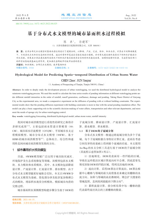
基于分布式水文模型的城市暴雨积水过程模拟
收稿日期:2021-04-15。
项目来源:天津市重点研发计划院市合作计划项目 (18YFYSZC00120)。
Copyright©博看网. All Rights Reserved.
· 106 ·
第20 卷第 8 期
地理空间信息
加载 DEM
填洼
无洼地
DEM
流向计算
累积流量
计算
栅格转换
为矢量
河网计算
子流域划分
CHEN Zhuo1, SUN Jianjun1
(1. Academy of Prospecting of Tianjin, Tianjin 300191, China)
Abstract: In order to deeply study the development process of urban waterlogging, we used the distributed hydrological model to analyze the
渍水点.shp 属性表 (部分)
FID
Shape
1
Point
0
2
Point
Point
Area
Address
花溪区
甲秀南路与溪北路交叉口吉林村拉槽
花溪区
黔灵山路黔灵山隧道 B 匝道
南明区
机场路小碧立交桥下交叉口积水点
X
Y
665 966.716 1
2 926 580.102 3
678 860.232 6
q = Kq 0 + q 0
'
(6)
积水模型
Q z = å[(Qi −q × Si)× Dti]
式中, q 为排水效率,单位为 m3 / (s × km 2 ) ; q 0 为设
艺传毕业设计论文-《通天塔》电影中的时空结构特色分析

毕业论文开题报告论文题目:《通天塔》电影中的时空结构特色分析学生姓名:XXX学号:1008611二级学院名称:电视艺术学院专业:电视节目制作指导教师:XXX职称:讲师填表日期:2014年12月28日浙江传媒学院教务处制一、选题的背景与意义:电影是叙事的艺术,并且是大众艺术。
那么这样的叙事首先就要让人们懂得,这是大众艺术的前提。
因此就要有清晰的叙述线和逻辑线。
叙述线的设置要符合观赏者的习惯,在叙述线中还要尽可能提高信息传递的有效性,并减少对有用信息的干扰。
时间的运动线和空间的运动线是叙事线的两条主干。
要正确地完成叙述任务,时间线和空间线就必须明确、清晰。
时空结构是电影中最主要的故事架构。
一部电影如果时空关系发生了混乱,就必然造成理解上的失误。
因此,无论是对于剧本的写作,还是镜头表现性、镜头的剪辑以及蒙太奇制作都离不开对时间结构、空间结构的描写与准确表现。
因此,电影又是一种时空的表现艺术。
2006 年由墨西哥导演冈萨雷斯•伊纳里多执导的影片《通天塔》,借用了《圣经》中“通天塔”的典故为影片命名,向我们揭示了一个跨越时间和空间局限的,拥有普世价值的主题:人类由于缺乏沟通、理解和信任从而造成了许多小到普通家庭,大到国家民族的冲突和争端。
导演冈萨雷斯•伊纳里多以此片对人类命运的深刻思考和此片所揭示的深刻而具有普世性的主题获得了金球奖最佳剧情片奖、戛纳电影节最佳导演奖等多项大奖。
而用来承载和体现这一宏大主题的故事情节也是非常的庞大和复杂。
影片由涉及三个大洲,分别发生在摩洛哥、美国、日本和墨西哥四个国家的四个故事组成。
这些故事涉及到因沟通不佳而导致的各种矛盾,它们互相平行发展,又有所交叉,是如此的纷繁复杂。
本片导演采用了交错式的多重时空结构,将这些纷繁复杂的故事建构到了影片独特的艺术时空之中,使之成为一个艺术整体,从而很好地呈现了影片深刻的人文主题,而这种独特的时空结构也成为了影片成功的关键因素。
二、研究的基本内容与拟解决的主要问题:1、时空交错式剧作结构由多条叙事线索组成,每条叙事线索都具有相对独立性,可以独立成篇,其间人物角色不同,故事情节无重叠之处,并且发生发展有头有尾,有因有果,逻辑严密。
秦川牛FADS基因家族克隆、生物信息学分析及组织表达研究
中国畜牧兽医 2024,51(3):903-915C h i n aA n i m a lH u s b a n d r y &V e te r i n a r y Me d i c i n e 秦川牛F A D S 基因家族克隆㊁生物信息学分析及组织表达研究尹思琦,赵刚奎,高海旭,孙红红,辛怡然,昝林森,赵春平(西北农林科技大学动物科技学院,杨凌712100)摘 要:ʌ目的ɔ试验旨在系统分析秦川牛脂肪酸去饱和酶(F A D S )基因家族,阐明该家族成员在秦川牛不同组织及脂肪细胞不同分化时期的时空表达规律,为进一步探究其在牛脂肪沉积中的作用奠定基础㊂ʌ方法ɔ试验采集秦川牛不同组织样本,从肾周脂肪中分离前体脂肪细胞,通过P C R 扩增F A D S 基因家族C D S 区序列,利用生物信息学软件分析预测其序列特征㊂利用实时荧光定量P C R 检测F A D S 基因家族成员在成年牛不同组织及肾周前体脂肪细胞分化过程中的时空表达谱㊂ʌ结果ɔ试验成功扩增出F A D S 基因家族3个成员(F A D S 1㊁F A D S 2和F A D S 3)C D S 区,大小分别为1425㊁1335㊁1332b p㊂系统进化树结果显示,秦川牛F A D S 基因家族成员氨基酸序列与瘤牛相似性最高,与小鼠的亲缘关系较远㊂生物信息学预测结果显示,F A D S 基因家族均为较稳定的亲水性蛋白,二级结构主要由α-螺旋构成,三级结构与二级结构预测结果一致㊂F A D S 1和F A D S 2主要定位于内质网(44.4%㊁44.4%),F A D S 3主要定位细胞膜中(39.1%)㊂实时荧光定量P C R 结果显示,F A D S 1㊁F A D S 3基因在肌肉组织表达量较高,F A D S 2基因在肝脏中表达量最高,显著高于其他组织(P <0.05)㊂在脂肪细胞的成脂分化过程中,与其他时间点相比,F A D S 1和F A D S 2基因在第2天时表达量最高(P <0.05),F A D S 3基因则在第2天时表达量最低(P <0.05)㊂ʌ结论ɔ本研究成功克隆了秦川牛F A D S 基因家族成员F A D S 1㊁F A D S 2㊁F A D S 3,在瘤牛㊁山羊㊁绵羊等哺乳动物中高度保守㊂F A D S 基因家族均为较稳定的亲水性蛋白,F A D S 1㊁F A D S 3基因在肌肉组织中高表达,F A D S2基因在肝脏组织中高表达㊂在脂肪细胞的成脂分化过程中,分化第2天时,F A D S 1㊁F A D S 2基因表达量最高,F A D S 3基因表达量最低㊂试验结果进一步揭示F A D S 基因家族通过调控脂肪细胞分化进而影响肉牛脂肪沉积作用机制研究奠定基础㊂关键词:秦川牛;F A D S 基因家族;生物信息学;表达中图分类号:S 823文献标识码:AD o i :10.16431/j .c n k i .1671-7236.2024.03.002 开放科学(资源服务)标识码(O S I D ):收稿日期:2023-09-22基金项目:陕西省农业科技创新驱动项目(N Y K J -2022-Y L (X N )03);陕西省重点研发计划项目 两链 融合重点专项(2022G D -T S L D -46-0404)联系方式:尹思琦,E -m a i l :h i y i n s i q i @163.c o m ㊂通信作者赵春平,E -m a i l :z h a o .c h u n p i n g@f o x m a i l .c o m C l o n i n g ,B i o i n f o r m a t i c sA n a l y s i s a n dT i s s u eE x pr e s s i o no f F A D S G e n eF a m i l yi n Q i n c h u a nC a t t l e Y I NS i q i ,Z H A OG a n g k u i ,G A O H a i x u ,S U N H o n g h o n g ,X I N Y i r a n ,Z A NL i n s e n ,Z H A OC h u n p i n g(C o l l e g e o f A n i m a l S c i e n c e a n dT e c h n o l o g y ,N o r t h w e s t A &FU n i v e r s i t y ,Y a n g l i n g 712100,C h i n a )A b s t r a c t :ʌO b j e c t i v e ɔT h e p u r p o s e o f t h i s e x p e r i m e n tw a s t o s y s t e m a t i c a l l y a n a l y z e t h e f a t t y ac id de s a t u r a s e s (F A D S )g e n ef a m i l y i n Q i n c h u a n c a t t l e ,c l a r i f y t h e s p a t i o t e m p o r a le x pr e s s i o n p a t t e r n s o f t h e s em e m b e r s i nv a r i o u s t i s s u e s a n dd i f f e r e n t d i f f e r e n t i a t i o n s t a g e s o f p r e a d i p o c yt e s ,a n d l a y a f o u n d a t i o n f o r f u r t h e r e x p l o r i n g t h e f u n c t i o n a n d r e g u l a t o r y r o l e s o f F A D S g e n e f a m i l yi nb o v i n e f a t d e p o s i t i o n .ʌM e t h o d ɔD i f f e r e n t t i s s u e s a m p l e s o fQ i n c h u a n c a t t l ew e r e c o l l e c t e d ,t h e p r e a d i p o c y t e sw e r ei s o l a t e df r o m p e r i r e n a lf a t ,a n dt h e C D Sr e g i o ns e qu e n c e so f F A D S g e n e f a m i l y w e r e a m p l i f i e db y P C R ,a n d t h e s e q u e n c e c h a r a c t e r i s t i c sw e r e p r e d i c t e db y b i o i n f o r m a t i c s s o f t w a r e .R e a l -t i m e q u a n t i t a t i v e P C R w a su s e dt od e t e c tt h et e m p o r a la n ds p a t i a le x p r e s s i o n p r o f i l e so f F A D S g e n ef a m i l y m e m b e r si n d i f f e r e n tt i s s u e s o fa d u l tc a t t l e a n d d u r i n g th e中国畜牧兽医51卷d i f f e r e n t i a t i o no f p r e r e n a la d i p o c y t e s.ʌR e s u l tɔT h eC D Sr e g i o no f3m e m b e r so f F A D S g e n e f a m i l y(F A D S1,F A D S2a n dF A D S3)w a s a m p l i f i e d s u c c e s s f u l l y w i t h t h e s i z e o f1425,1335a n d 1332b p,r e s p e c t i v e l y.T h e p h y l o g e n e t i ct r e er e s u l t ss h o w e dt h a tt h ea m i n oa c i ds e q u e n c e so f F A D S g e n e f a m i l y m e m b e r so fQ i n c h u a nc a t t l eh a d t h eh i g h e s t s i m i l a r i t y w i t h B o s i n d i c u s,a n d w e r e f a r r e l a t e d t o M u s m u s c u l u s.T h e r e s u l t s o f b i o i n f o r m a t i c s p r e d i c t i o n s h o w e d t h a t t h e F A D S g e n e f a m i l y w e r e s t a b l e h y d r o p h i l i c p r o t e i n s,a n d t h e s e c o n d a r y s t r u c t u r ew a sm a i n l y c o m p o s e d o f a l p h ah e l i x,a n dt h et e r t i a r y s t r u c t u r e w a sc o n s i s t e n t w i t ht h e p r e d i c t e ds e c o n d a r y s t r u c t u r e.F A D S1a n dF A D S2w e r em a i n l y l o c a t e d i nt h ee n d o p l a s m i c r e t i c u l u m(44.4%a n d44.4%),a n d F A D S3w a sm a i n l y l o c a t e di nt h ec e l lm e m b r a n e(39.1%).R e a l-t i m e q u a n t i t a t i v eP C Rr e s u l t s s h o w e d t h a t t h ee x p r e s s i o no f F A D S1a n d F A D S3g e n e sw e r eh i g h e r i n m u s c l e t i s s u e,a n dt h e e x p r e s s i o no f F A D S2g e n ew a s t h eh i g h e s t i n l i v e r,a n ds i g n i f i c a n t l y h i g h e r t h a nt h a t i no t h e r t i s s u e s(P<0.05).W i t h t h e a d i p o g e n i c d i f f e r e n t i a t i o n o f a d i p o c y t e s,c o m p a r e d t o o t h e rd i f fe r e n t i a t i o n t i m e,t h e e x p r e s s i o n of F A D S1a n d F A D S2g e n e sw e r e th e hi g h e s t o n d a y s2(P<0.05),w h i l e t h e e x p r e s s i o no f F A D S3g e n ew a s t h e l o w e s t o nd a y s2(P<0.05).ʌC o n c l u s i o nɔF A D S1,F A D S2a n d F A D S3o f F A D S g e n e f a m i l y i nQ i n c h u a n c a t t l ew e r e s u c c e s s f u l l y c l o n e d, w h i c hw e r eh i g h l y c o n s e r v e d B o s i n d i c u s,C a p r ah i r c u s a n d O v i sa r i e s a n do t h e r m a m m a l s.F A D S g e n e f a m i l y w e r er e l a t i v e l y s t a b l eh y d r o p h i l i c p r o t e i n s,F A D S1a n d F A D S3g e n e sw e r e h i g h l y e x p r e s s e d i n m u s c l e,a n d F A D S2g e n ew a sh i g h l y e x p r e s s e di nl i v e r.I nt h e p r o c e s so f a d i p o g e n i c d i f f e r e n t i a t i o no f a d i p o c y t e s,F A D S1a n d F A D S2g e n ee x p r e s s i o n sw e r e t h eh i g h e s t a n d F A D S3g e n ee x p r e s s i o n w a st h el o w e s to nd a y s2o fd i f f e r e n t i a t i o n.T h er e s u l t sl a i da f o u n d a t i o n f o r f u r t h e r r e s e a r c ho n t h em e c h a n i s mo f F A D S g e n e f a m i l y i n f l u e n c i n g f a t d e p o s i t i o n i nb e e f c a t t l eb y r e g u l a t i n g a d i p o c y t e d i f f e r e n t i a t i o n.K e y w o r d s:Q i n c h u a n c a t t l e;F A D S g e n e f a m i l y;b i o i n f o r m a t i c s;e x p r e s s i o n多不饱和脂肪酸(P U F A s)是重要的多功能介质,可改善和维持机体健康[1-3]㊂P U F A s包括ω-6和ω-3P U F A,具有维持细胞膜流动性㊁减少单核细胞/巨噬细胞分泌促炎细胞因子㊁降低对心脏室性节律失常的易感性㊁改善血管内皮细胞的功能,抑制血小板聚集和减少肝脏中的甘油三酯合成等生物学作用[3-4]㊂其中长链多不饱脂肪酸(L C P U F A s)包含由18~22个碳原子组成的碳链,并且含有两个或两个以上双键的直链脂肪酸[5],是人体自身不能合成,但在生长发育过程中必需的脂肪酸㊂现有研究表明,具有功能的L C P U F A s主要包括二十碳四烯酸(A A)㊁二十二碳六烯酸(D H A)以及二十碳五烯酸(E P A),其发挥的生理功能包括促进视网膜和大脑发育㊁预防和治疗心血管疾病㊁炎症免疫的调节作用㊁抗肿瘤作用以及影响凝血功能和调节血脂等[5-6]㊂脂肪酸去饱和酶(F A D S)是L C P U F A s合成过程中的关键酶之一,该家族包括3个成员:F A D S1㊁F A D S2㊁F A D S3,同在人类11号染色体上[7]㊂其中F A D S1与F A D S2分别编码Δ5与Δ6去饱和酶[8],二者在P U F A s合成中可在脂肪酸碳链上的碳原子之间加入双键,发挥调控作用[9]㊂F A D S1和F A D S2基因作为早期生长和肥胖的候选标志物被广泛研究[10-11],其中F A D S1基因可以在油酸代谢中参与Δ7去饱和作用,使11-20ʒ1生成7,11-20ʒ2[12],还能通过AM P K/S R E B P1途径调节山羊乳腺上皮细胞脂肪酸合成和甘油三酯积累[13]㊂同时沉默F A D S1基因可抑制黑色素细胞(P I G1)的增殖并诱导细胞死亡[14]㊂另外,F A D S2基因缺陷型小鼠的体重较正常小鼠减少20%~25%,体脂含量较低,且对胰岛素敏感性降低[15];在山羊乳腺上皮细胞中干扰F A D S2基因表达可明显降低过氧化物酶体增殖物激活受体α(P P A Rα)和转录因子类固醇调节元件结合蛋白1(S R E B P1)的表达[16]㊂此外,F A D S1基因的亚型也可以增强F A D S2基因介导的前体脂肪酸生成[17]㊂目前关于F A D S3基因的研究较少,除了其对肝脏和大脑中的二十二碳六烯酸存在调节作用外[18],进一步的研究表明F A D S3是一种Δ14Z 鞘样碱性去饱和酶,在女性血浆中活性更高,与人血浆鞘脂体中的性别特异性差异有关[19]㊂上述研究表明,F A D S基因家族很可能通过与转录因子结合或参与P P A R s通路等途径参与脂肪的发育调控㊂目前,关于F A D S基因家族功能的研究大多集中在4093期尹思琦等:秦川牛F A D S基因家族克隆㊁生物信息学分析及组织表达研究人类早期发育和对母乳的影响方面,在成脂分化及脂代谢方面的研究也多以小鼠㊁山羊等为研究对象㊂关于牛F A D S基因家族基本信息及其调控脂肪沉积方面的研究鲜有报道㊂本研究对秦川牛F A D S 基因家族蛋白进行生物信息学预测,并对其在成年牛不同组织及牛脂肪细胞成脂分化中的表达规律进行分析,为进一步研究F A D S基因家族在牛脂肪沉积中的作用及调控机制提供参考㊂1材料与方法1.1样本采集试验所用秦川牛组织样品采自西北农林科技大学良繁场的成年秦川母牛㊂屠宰过程中,用无菌手术器械分别采集秦川牛13个部位的组织样品(心脏㊁肺脏㊁肾脏㊁肝脏㊁脾脏㊁小肠㊁皮下脂肪㊁肾周脂肪㊁心包脂肪㊁肠系膜脂㊁背最长肌㊁前腿肌㊁后腿肌),放入无菌㊁无R N A酶㊁无D N A酶的冻存管中,液氮速冻后―80ħ保存备用㊂1.2主要试剂及仪器胰蛋白酶购自C y t i v a公司;胰岛素㊁D X M S㊁I B M X㊁R o s i g l i t a z o n e均购自S i g m a-A l d r i c h(上海)公司;胎牛血清购自P A N公司;M5T a q H i F iP C R M i x购自北京聚合美生物科技有限公司;D E M E/ F-12培养基㊁青霉素/链霉素双抗均购自H y C o l n e公司,T r i z o l㊁P r i m e S c r i p t T M R T R e a g e n tK i tw i t h g D N A E r a s e r㊁D L2000D N A M a r k e r均购自T a k a R a公司;G e l E x t r a c t i o nK i t购自O m e g a公司㊂水浴锅购自上海精宏公司;C O2细胞培养箱购自T h e r m o公司;荧光定量P C R仪购自A p p l i e dB i o s y s t e m s公司㊂1.3秦川牛前体脂肪细胞的分离培养及诱导分化用手术剪和镊子去除新鲜采集的秦川牛肾周脂肪组织表面的肌肉㊁结缔组织以及血管等杂质,将脂肪组织修剪成约1m m3大小的组织块,用P B S缓冲液冲洗3次,使用Ⅰ型胶原酶对组织块进行消化,加入等量的完全培养基终止消化㊂使用0.25和0.075m m网筛对混合液分别过滤2次,收集滤液, 1000r/m i n离心15m i n,弃去上清㊂用完全培养基重悬沉淀,37ħ㊁5%C O2培养箱中培养㊂2h后更换新鲜的完全培养基,可见有部分贴壁细胞,即获得前体脂肪细胞㊂将原代牛前体脂肪细胞接种于6孔板,置37ħ㊁5%C O2培养箱培养至细胞汇合度达80%,加入诱导Ⅰ液(基础培养液中含0.5m m o l/L I B M X㊁2μm o l/L胰岛素㊁1μm o l/L地塞米松㊁1μm o l/L罗格列酮),诱导2d后更换诱导Ⅱ液(基础培养液中含2μm o l/L胰岛素),之后每2d更换1次诱导Ⅱ液㊂1.4引物设计及合成根据G e n B a n k中公布的牛F A D S1(X M_ 005226961.4)㊁F A D S2(NM_001083444.1)㊁F A D S3(NM_001083691.2)基因序列,采用P r i m e r P r e m i e r5.0软件设计引物,引物序列见表1㊂引物均由北京擎科生物科技有限公司合成㊂表1引物序列信息T a b l e1P r i m e r s e q u e n c e i n f o r m a t i o n基因G e n e s引物序列P r i m e r s e q u e n c e s(5'ң3')退火温度A n n e a l i n gt e m p e r a t u r e/ħ产物大小P r o d u c tl e n g t h/b p用途P u r p o s eF A D S1F:A TG G G G G A C G C G C G C C G57.391425克隆R:T T A T T G G T G G A G A T A G G C A T C T A GF A D S2F:A TG G G G A A G G G G G G A A A C C A63.061335克隆R:T C A T T T G T G G A G G T A G G C G T CF A D S3F:A TG G G C G G T G T C G G G G A G C67.191332克隆R:T C A C T G G T G G A G G T A G G C T T C C A G C CF A D S1F:C TG C T T T G G T G C C A T A A C C C59.47118实时荧光定量P C RR:C T C A G C C T T C G C T G A C A T T GF A D S2F:T T C CG C T G G G A G G A G A T T C58.79188实时荧光定量P C RR:C G C A C A A A A T C A A G G T T G C GF A D S3F:TG A T C T A C A T G C T T G G C C C C64.89303实时荧光定量P C RR:T C T T G C C G T A C T C A A C G G A Cβ-a c t i n F:T C T A G G C G G A C T G T T A G C50.7082实时荧光定量P C R R:C C A T G C C A A T C T C A T C T C G509中国畜牧兽医51卷1.5总R N A提取及c D N A合成取成年秦川牛心脏㊁肺脏㊁肾脏等13个组织及不同分化天数(第0㊁2㊁4㊁6天)牛前体脂肪细胞,采用T r i z o l法提取组织及细胞总R N A,按照P r i m e S c r i p tR T R e a g e n tK i tw i t h g D N A E r a s e r反转录试剂盒的操作步骤,将其反转录为c D N A,―20ħ保存备用㊂1.6F A D S基因家族克隆及测序以秦川牛肾周脂肪细胞c D N A为模板,通过P C R扩增F A D S基因家族C D S序列㊂P C R反应体系20μL:M5T a q H i F i P C R M i x(2ˑ)10μL,上㊁下游引物(10μm o l/L)各1μL,c D N A(100n g/μL) 2μL,R N a s e-f r e ed d H2O6μL㊂P C R反应程序: 95ħ预变性5m i n;94ħ变性30s,退火(退火温度见表1)40s,72ħ延伸50s,共35个循环;72ħ延伸10m i n㊂P C R产物经1.0%琼脂糖凝胶电泳检测后进行切胶回收,P C R产物纯化后送至北京擎科生物技术有限公司测序,将测序结果与N C B I数据库中的核苷酸序列进行比对分析㊂1.7相似性比对及系统进化树构建通过N C B I官网查询F A D S基因家族氨基酸序列,利用M e g aX软件将秦川牛F A D S基因家族的氨基酸序列与瘤牛㊁水牛㊁山羊㊁绵羊㊁人㊁恒河猴㊁小鼠㊁马㊁黑猩猩㊁鸡的氨基酸序列进行相似性比对,并通过邻接法构建系统进化树㊂1.8生物信息学分析测序结果通过B L A S T比对后,在N C B I中查询获得氨基酸序列,利用生物信息学在线工具预测F A D S基因家族的蛋白理化性质㊁亲/疏水性㊁磷酸化位点等特征,具体软件信息见表2㊂表2生物信息学分析软件T a b l e2B i o i n f o r m a t i c s a n a l y s i s t o o l s在线工具O n l i n e t o o l s网址W e b s i t e s功能预测F u n c t i o n p r e d i c t i o n P r o t P a r m h t t p s:ʊw e b.e x p a s y.o r g/p r o t p a r a m/理化性质P r o t S c a l e h t t p s:ʊw e b.e x p a s y.o r g/p r o t s c a l e/亲/疏水性N e t P h o s3.1S e r v e r h t t p s:ʊs e r v i c e s.h e a l t h t e c h.d t u.d k/s e r v i c e.p h p?N e t P h o s-3.1磷酸化位点P S O R TⅡP r e d i c t h t t p s:ʊp s o r t.h g c.j p/f o r m2.h t m l亚细胞定位M E M E h t t p s:ʊm e m e-s u i t e.o r g/m e m e/t o o l s/m e m e潜在保守性基序P r a b i h t t p s:ʊn p s a-p r a b i.i b c p.f r/c g i-b i n/n p s a_a u t o m a t.p l?p a g e=/N P S A/n p s a_s e c c o n s.h t m l二级结构S W I S S-MO D E L h t t p s:ʊs w i s s m o d e l.e x p a s y.o r g/i n t e r a c t i v e三级结构G e n eMA N I A h t t p:ʊg e n e m a n i a.o r g/蛋白互作网络1.9秦川牛F A D S基因家族在不同组织及不同分化时期前体脂肪细胞中的表达通过实时荧光定量P C R检测F A D S基因家族在秦川牛不同组织和不同分化阶段前体脂肪细胞中的表达特性,引物信息见表1㊂P C R反应体系20μL:G r e e n P r e m i xE x T a qⅡ(T l i R N a s e HP l u s)(2ˑ)10μL,上㊁下游引物(10μm o l/L)各1μL,c D N A(100n g/μL)2μL, R N a s e-f r e eH2O6μL㊂P C R反应程序:95ħ预变性30s;95ħ变性15s,退火(退火温度见表1)15s, 72ħ延伸60s,共39个循环㊂以β-a c t i n为内参基因,试验重复3次,用2-әәC t法计算目的基因的相对表达量㊂1.10数据统计分析使用G r a p h P a dP r i s m9.0软件进行分析和作图,通过O n e-W a y A N O V A进行单因素方差分析,利用独立样本t检验分析差异显著性,结果以平均值ʃ标准差表示,P<0.05表示差异显著㊂2结果2.1秦川牛F A D S基因家族克隆及分析P C R扩增产物经1.0%琼脂糖凝胶电泳检测显示,条带单一㊁清晰,与预期扩增片段大小相符(图1),表明成功获得F A D S基因家族成员C D S序列㊂使用N C B I B L A S T对测序结果进行比对分析,结果显示秦川牛F A D S1㊁F A D S2㊁F A D S3基因的C D S序列长度分别为1425㊁1335㊁1332b p,与G e n B a n k中相应序列一致㊂2.2相似性比对及系统进化树构建将牛F A D S基因家族氨基酸序列分别与不同物种进行序列比对,秦川牛F A D S1㊁F A D S2和F A D S3基因氨基酸序列与瘤牛相似性分别为100%㊁97%和91%㊂系统进化树结果显示,秦川牛F A D S基因家族与瘤牛㊁山羊㊁绵羊等物种亲缘关系较近,与小鼠的亲缘关系较远(图2)㊂6093期尹思琦等:秦川牛F A D S 基因家族克隆㊁生物信息学分析及组织表达研究1㊁2,F A D S 1基因P C R 扩增产物;M ,D L 2000D N A M a r k e r ;3㊁4,F A D S 2基因P C R 扩增产物;5㊁6,F A D S 3基因P C R 扩增产物1a n d 2,F A D S 1g e n eP C Ra m p l i f i c a t i o n p r o d u c t s ;M ,D L 2000D N A M a r k e r ;3a n d 4,F A D S 2g e n eP C Ra m pl i f i c a t i o n p r o d u c t s ;5a n d6,F A D S 3g e n eP C Ra m p l i f i c a t i o n p r o d u c t s 图1 秦川牛F A D S 基因家族P C R 扩增结果F i g .1 P C Ra m p l i f i c a t i o n r e s u l t s o f F A D S g e n e f a m i l yi n Q i n c h u a n c a t t le 图2 秦川牛F A D S 基因家族氨基酸序列系统进化树F i g .2 P h y l o g e n e t i c t r e e o f a m i n o a c i d s e q u e n c e o f F A D S g e n e f a m i l yi n Q i n c h u a n c a t t l e 709中 国 畜 牧 兽 医51卷2.3 生物信息学分析2.3.1 理化性质分析 使用P r o t P a r m 在线程序预测F A D S 基因家族理化性质,结果见表3,秦川牛F A D S 基因家族编码443~474个氨基酸,原子总数为7209~7761个,蛋白分子质量为51306.35~54974.17u ;理论等电点预测范围为8.28~9.75,表明该家族成员整体偏碱性㊂氨基酸残基中占比重最高的均为亮氨酸,半胱氨酸占比最低㊂F A D S 2蛋白不稳定系数为40.89(最稳定),F A D S 1和F A D S 3蛋白为不稳定蛋白㊂F A D S 家族蛋白脂肪族指数均较高,理化性质差异不大,较为稳定㊂表3 秦川牛F A D S 基因家族理化性质T a b l e 3 P h y s i c a l a n d c h e m i c a l p r o p e r t i e s o f F A D S g e n e f a m i l y i n Q i n c h u a n c a t t l e 蛋白P r o t e i n s 氨基酸数量A m i n o a c i dn u m b e r/个分子质量M o l e c u l a rw e i g h t /u 分子式F o r m u l a 理论等电点P I不稳定系数I n s t a b i l i t yi n d e x 脂肪族指数A l i ph a t i c i n d e x F A D S 147454974.17C 2559H 3862N 694O 628S 189.7548.9491.75F A D S 244452532.59C 2452H 3632N 644O 622S 148.9940.8986.58F A D S 344351306.35C 2380H 3569N 641O 604S 158.2852.7193.592.3.2 亲/疏水性分析 通过在线程序P r o t S c a l e 分析F A D S 基因家族的亲/疏水性,结果见图3,F A D S 1疏水性最大值为2.891,其中异亮氨酸(I l e )的单个值最高,为4.500;最小值为―3.091㊂F A D S 2疏水性最大值为2.444,其中I l e 的单个值最高(4.500);最小值为―2.800㊂F A D S 3疏水性最大值为2.867,最小值为―3.022㊂推测F A D S基因家族均为亲水性蛋白㊂A~C ,分别为F A D S 1㊁F A D S 2和F A D S 3基因㊂图4㊁6㊁7㊁9同A -C ,F A D S 1,F A D S 2a n d F A D S 3g e n e s ,r e s p e c t i v e l y .T h e s a m e a s f i g .4,f i g .6,f i g .7a n d f i g .9图3 秦川牛F A D S 基因家族亲/疏水性预测F i g .3 H y d r o p h i l i c i t y a n dh y d r o p h o b i c i t yp r e d i c t i o no f F A D S g e n e f a m i l yi n Q i n c h u n c a t t l e 2.3.3 磷酸化位点预测 利用N e t ph o s3.1S e r v e r 在线软件预测F A D S 基因家族的磷酸化位点,结果见图4,F A D S 1蛋白中共预测到29个潜在磷酸化修饰位点,其中包括17个丝氨酸(S e r )磷酸化位点㊁10个苏氨酸(T h r )磷酸化位点㊁2个酪氨酸(T yr )磷酸化位点;F A D S 2蛋白中共预测到潜在磷酸化修饰位点28个,其中包括S e r 磷酸化位点15个㊁T h r 磷酸化位点11个㊁T yr 磷酸化位点2个;F A D S 3蛋白中共预测到潜在磷酸化修饰位点21个,其中包括S e r 磷酸化位点14个㊁T h r 磷酸化位点4个㊁T yr 磷酸化位点3个㊂2.3.4 亚细胞定位分析 通过P S O R T ⅡP r e d i c t i o n 在线软件预测秦川牛F A D S 基因家族亚细胞定位,结果见表4㊂秦川牛F A D S 1㊁F A D S 2蛋白分布于内质网的可能性均为44.4%,F A D S 1蛋白在细胞质㊁线粒体㊁高尔基体以及细胞膜中分布的可能性为11.1%,F A D S 2蛋白在细胞膜或线粒体中的可能为22.2%,而F A D S 3蛋白最可能在细胞膜中(39.1%),其次是内质网(38.4%)㊂8093期尹思琦等:秦川牛F A D S 基因家族克隆㊁生物信息学分析及组织表达研究图4 秦川牛F A D S 基因家族磷酸化位点预测F i g .4 P r e d i c t i o no f p h o s p h o r y l a t i o n s i t e s o f F A D S g e n e f a m i l y i n Q i n c h u a n c a t t l e 表4 秦川牛F A D S 基因家族亚细胞定位预测T a b l e 4 P r e d i c t i o no f s u b c e l l u l a r l o c a l i z a t i o no f F A D S g e n e f a m i l y i n Q i n c h u n c a t t l e %亚细胞定位S u b c e l l u l a r l o c a l i z a t i o n 占比P e r c e n t a ge F A D S 1F A D S 2F A D S 3内质网E n d o p l a s m i c r e t i c u l u m 44.444.438.4细胞质C y t o p l a s m i c 11.122.2线粒体M i t o c h o n d r i a l11.122.213.0高尔基体G o l g i 11.14.3空泡V a c u o l a r 11.1细胞膜P l a s m am e m b r a n e 11.139.1分泌系统的囊泡V e s i c l e s o f s e c r e t o r y s ys t e m 11.14.3细胞外E x t r a c e l l u l a r4.32.3.5 保守基序及基因结构分析 利用M E M E在线软件预测F A D S 基因家族潜在的保守性基序,结果见图5,与F A D S 2㊁F A D S 3相比,F A D S 1最前端缺少一个M o t i f 元件,F A D S 2与F A D S 3的M o t i f元件数量和顺序均保持一致(图5A )㊂基序结构图中,横轴表示碱基序号,纵轴表示校正后得分,碱基高度越高表示该位置出现这种碱基可能性越高,F A D S 基因家族具有较高保守性(图5B )㊂2.3.6 二级结构预测 利用在线软件P r a b i 对F A D S 基因家族进行二级结构预测分析,通过不同算法对二级结构分类预测(D S C )㊁多变量线性回归组合预测(M L R C )㊁神经网络预测(P H D )和综合预测(S e c .C o n s .)计算α-螺旋㊁延伸链㊁无规则卷曲等在蛋白结构中的占比,结果见表5,F A D S 基因家族二级结构占比变化不大,主要由α-螺旋和无规则卷曲构成㊂909中 国 畜 牧 兽 医51卷图5 秦川牛F A D S 基因家族保守基序(A )及基序结构(B )F i g .5 C o n s e r v e dm o t i f (A )a n dm o t i f s t r u c t u r e (B )o f F A D S g e n e f a m i l y i n Q i n c h u a n c a t t l e 表5 秦川牛F A D S 基因家族二级结构预测T a b l e 5 P r e d i c t i o no f s e c o n d a r y s t r u c t u r e o f F A D S g e n e f a m i l y i n Q i n c h u a n c a t t l e %项目I t e m s 基因G e n e s占比P e r c e n t a ge α-螺旋A l p h ah e l i x 延伸链E x t e n d e d s t r a n d无规则卷曲R a n d o mc o i l 模棱两可状态T h e a m b i g u o u s s t a t e o f b e i n gD S CF A D S 137.133.3859.490F A D S 245.720.9053.380F A D S 342.982.7154.400M L R CF A D S 149.587.7143.250F A D S 252.7011.2636.040F A D S 352.6010.3837.020P H DF A D S 154.018.2337.760F A D S 257.886.3135.810F A D S 360.956.5532.510S e c .C o n s .F A D S 149.585.2743.251.90F A D S 252.034.2840.093.60F A D S 353.504.9738.153.392.3.7 三级结构预测 利用S W I S S -MO D E L 软件通过同源建模法进一步预测F A D S 基因家族三级结构,可视化结果见图6㊂F A D S 基因家族三级结构与二级结构预测结果基本一致㊂2.3.8 蛋白互作分析 通过基因富集分析以及在线网站预测,绘制F A D S 基因家族蛋白互作网络,结果见图7㊂F A D S 1㊁F A D S 2均与超长链脂肪酸蛋白5(E l o v l 5)㊁E l o v l 2存在相互作用;三者和硬0193期尹思琦等:秦川牛F A D S 基因家族克隆㊁生物信息学分析及组织表达研究脂酰辅酶A 去饱和酶5(S C D 5)共享蛋白质结构域,且F A D S 2参与P P A R s 信号通路,推测三者可能参与脂质的合成与运输,且存在相互作用㊂图6 秦川牛F A D S 基因家族三级结构预测F i g .6 P r e d i c t i o no f t e r t i a r y s t r u c t u r e o f F A D S g e n e f a m i l yi n Q i n c h u a n c a t t l es 图7 秦川牛F A D S 基因家族蛋白互作网络图F i g .7 P r o t e i n i n t e r a c t i o nn e t w o r ko f F A D S g e n e f a m i l yi n Q i n c h u a n c a t t l e 119中国畜牧兽医51卷2.4F A D S基因家族在秦川牛不同组织中的表达由表6可知,F A D S基因家族在前腿肌㊁后腿肌㊁背最长肌均有较高表达,F A D S1基因在心包脂中不表达;F A D S1㊁F A D S2基因均在肠系膜脂高表达,在肾周脂中表达量较低;F A D S3则在肾周脂中表达最高,在皮下脂肪中最低㊂另外F A D S1基因在后腿肌中表达量最高,脾脏中表达量最低,显著低于其他组织(P<0.05)㊂F A D S2基因在肝脏中表达量最高,显著高于其他组织(P<0.05)㊂F A D S3基因在前腿肌中表达量最高,显著高于除心脏外其他组织(P<0.05)㊂2.5F A D S基因家族在秦川牛不同分化时间前体脂肪细胞中的表达由图8可知,F A D S1和F A D S2基因在诱导分化第2天的前体脂肪细胞中表达量最高,显著高于其他时间点(P<0.05)㊂F A D S3基因则与之相反,在诱导分化第2天时表达量最低,显著低于其他时间点(P<0.05)㊂表6F A D S基因家族在秦川牛不同组织中的相对表达量T a b l e6R e l a t i v e e x p r e s s i o no f F A D S g e n e f a m i l y i nd i f f e r e n t t i s s u e s o f Q i n c h u n c a t t l e组织T i s s u e s F A D S1F A D S2F A D S3心脏H e a r t1.79ʃ0.08c3.72ʃ0.10b2.86ʃ0.05a肝脏L i v e r2.06ʃ0.33b10.96ʃ0.55a1.00ʃ0.07h脾脏S p l e e n1.00ʃ0.04f1.26ʃ0.05d1.46ʃ0.10f g肺脏L u n g1.96ʃ0.15b1.00ʃ0.06e2.35ʃ0.28b c肾脏K i n d e y2.19ʃ0.14b2.24ʃ0.19c2.07ʃ0.04c小肠S m a l l i n t e s t i n e1.63ʃ0.18c1.97ʃ0.03c d1.39ʃ0.07g背最长肌L o n g i s s i m u s d o r s im u s c l e1.57ʃ0.68b3.82ʃ0.30b2.66ʃ0.22a b前腿肌F o r e l e g m u s c l e2.26ʃ0.30a4.35ʃ0.39b3.73ʃ0.46a后腿肌H i n d l e g m u s c l e2.51ʃ0.03a4.02ʃ0.66b2.58ʃ0.02b肠系膜脂M e s e n t e r y i n t e r n a l f a t1.50ʃ0.14d2.97ʃ0.12b1.75ʃ0.18d e肾周脂P e r i r e n a l f a t1.19ʃ0.09e1.54ʃ0.36d1.82ʃ0.04d心包脂E p i c a r d i a l a d i p o s e 2.25ʃ0.08c d1.74ʃ0.13d e皮下脂肪S u b u t a n e o u s f a t1.37ʃ0.17e1.84ʃ0.12d1.72ʃ0.02e同列数据肩标不同字母表示差异显著(P<0.05);肩标相同字母表示差异不显著(P>0.05)I n t h e s a m e c o l u m n,v a l u e sw i t hd i f f e r e n t l e t t e r s u p e r s c r i p sm e a n s i g n i f i c a n t d i f f e r e n c e(P<0.05);W h i l ew i t h t h e s a m e l e t t e r s u p e r s c r i p t sm a e nn o s i g n i f i c a n t d i f f e r e n c e(P>0.05)3讨论F A D S基因家族作为重要的脂肪酸去饱和酶,首次在小鼠中成功克隆,随后在人㊁大鼠㊁奶山羊㊁鸡等物种中研究逐渐增多,通过对遗传和代谢组学的研究表明,F A D S基因家族中存在形成生物学重要脂质的关键控制点,且对组织特异性产生影响,在动物免疫㊁繁殖㊁生长发育等方面发挥着重要作用[20-21]㊂本研究以秦川牛为试验材料,克隆F A D S 基因家族成员C D S区,并对其进行理化性质分析,结果表明F A D S基因家族在哺乳动物中存在较高的保守性,F A D S1㊁F A D S2和F A D S3基因氨基酸序列与瘤牛相似性分别为100%㊁98%和97%,与水牛㊁山羊㊁绵羊等亲缘关系较近,结果与邬娇等[16]报道的奶山羊F A D S2基因研究一致㊂生物信息学分析表明,F A D S基因家族均为碱性亲水性蛋白,蛋白质总体折叠结构中亲水基团向外,疏水基团向内,并在跨膜区形成高疏水值区域,与蛋白二级结构㊁三级结构的预测结果一致㊂其中F A D S1基因与陈振鹏等[22]报道的碱地黑牛F A D S1基因的理化性质研究一致,但由于使用同源建模和折叠识别2种分析方法,对蛋白三级结构的预测有所不同;F A D S2基因与邬娇等[16]在奶山羊上的研究基本一致,亚细胞定位预测显示,F A D S1㊁F A D S2基因存在于内质网中几率较大,而F A D S3在细胞膜中的可能性最大㊂磷酸化位点预测显示F A D S基因家族存在大量的丝氨酸位点,丝氨酸在脂肪和脂肪酸的新陈代谢㊁肌肉生长㊁细胞膜制造加工㊁肌肉组织和包围神经细胞的鞘合成中均发挥作用[23],推测F A D S基因家族在细胞信号传递及脂质代谢中发挥着重要作用,其中F A D S1㊁F A D S2基因可能参与内质网中2193期尹思琦等:秦川牛F A D S 基因家族克隆㊁生物信息学分析及组织表达研究图8 F A D S 基因家族在秦川牛不同分化时间前体脂肪细胞中的相对表达量F i g .8 R e l a t i v e e x p r e s s i o no f F A D S g e n e f a m i l y a t d i f f e r e n t d i f f e r e n t i a t i o n t i m e s i n p r e a d i p o c yt e s o f Q i n c h u a n c a t t l e s 蛋白质与脂质的合成,F A D S 3基因则可能参与脂质转运或通过结合蛋白发挥作用㊂蛋白互作网络进一步分析显示,F A D S 1㊁F A D S 2㊁F A D S 3基因之间存在相互作用,且参与P P A R s 信号通路㊂相关研究表明F A D S 1可以增强F A D S 2介导的类花生酸前体脂肪酸的产生[17],且F A D S 1通过AM P K /S R E B P 1途径调节山羊乳腺上皮细胞脂肪酸合成和甘油三酯积累[13];F A D S 2则受S R E B P 1和P P A R α调控,从而影响鱼类长链多不饱和脂肪酸的合成[24-26];目前有关F A D S 3的研究较少,2017年Z h a n g 等[18]研究报道,F A D S 3基因敲除对小鼠肝脏和大脑中的二十二碳六烯酸起到调节作用,具体的调节机制仍有待探究㊂实时荧光定量P C R 检测F A D S 基因家族在秦川牛不同组织中的表达情况,结果发现F A D S 1㊁F A D S 3基因分别在后腿肌㊁前腿肌组织的表达量最高,而F A D S 2基因则在肝脏中表达量最高,其次是肌肉和心脏,在肺脏中表达量最低㊂相关研究报道,F A D S 1基因在奶山羊肌肉组织中表达量最高,F A D S 2基因在人脑和肝脏中高水平表达,在奶山羊肝脏组织中表达量最高[27-28]㊂肝脏是脂质合成㊁吸收和输出的主要器官,葡萄糖㊁脂类以及各种蛋白质转化为反应物为机体供能,F A D S 2基因高表达可能与脂质合成㊁肝脏基础代谢紧密相关㊂肌肉中存在大量游离脂肪酸和葡萄糖的转运[27],F A D S 1与F A D S 3基因在肌肉中高表达很可能参与其调控㊂同时,G l a s e r 等[21]研究表明,F A D S 3基因在山羊乳腺组织中表达量远高于肝脏,与本试验中F A D S 3基因在肝脏中低表达的结果一致㊂Y a n等[29]发现肠道菌群的改变会显著影响小鼠肠道和肝脏中F A D S 1㊁F A D S 2基因表达,本研究中不同部位脂肪组织中F A D S 1与F A D S 2基因在肠系膜脂中高表达,推测可能与此相关㊂F A D S 1㊁F A D S 2基因在秦川牛肾周前体脂肪细胞不同分化时间的表达量均呈现先上升后下降最后趋于平缓,而F A D S 3基因则相反,表现出先下降后上升趋势,说明F A D S 1㊁F A D S 2基因在脂肪细胞生长中发挥作用的进程一致,且符合脂肪细胞分化过程中标志基因表达变化的一般规律[30-32],二者可能存在相互调控,对脂肪细胞的分化产生影响㊂而F A D S 3基因发挥作用的时间与F A D S 1㊁F A D S 2不同,也可能与其发挥作用的时间或参与的信号通路不同相关联,后续需要进一步探究㊂319中国畜牧兽医51卷4结论本研究克隆了秦川牛F A D S基因家族成员F A D S1㊁F A D S2㊁F A D S3基因C D S区,大小分别为1425㊁1335㊁1332b p,该基因家族均为较稳定的亲水性蛋白,二级结构主要为α-螺旋,在瘤牛㊁山羊㊁绵羊等哺乳动物中高度保守㊂F A D S1㊁F A D S3基因在肌肉组织中高表达,F A D S2基因在肝脏组织中高表达㊂随着脂肪细胞的成脂分化,F A D S1㊁F A D S2基因在分化第2天表达量最高,F A D S3基因则与之相反㊂研究结果为进一步揭示F A D S基因家族功能及其在脂肪细胞分化和肉牛脂肪沉积的作用机制奠定基础㊂参考文献(R e f e r e n c e s):[1] K A P O O RB,K A P O O RD,G A U T AMS,e t a l.D i e t a r yp o l y u n s a t u r a t e d f a t t y a c i d s(P U F A s):U s e s a n dp o t e n t i a l h e a l t h b e n e f i t s[J].C u r r e n t N u t r i t i o nR e p o r t s,2021,10(3):232-242.[2] W I K T O R OW S K A A,B E R E Z I'N S K A M,N OWA KJ.P U F A s:S t r u c t u r e s,m e t a b o l i s m a n d f u n c t i o n s[J].A d v a n c e s i n C l i n i c a la n d E x p e r i m e n t a l M e d i c i n e,2015,24(6):931-941.[3] B A Z I N E T RP,L A YÉS.P o l y u n s a t u r a t e d f a t t y a c i d sa n d t h e i r m e t ab o l i t e s i n b r a i n f u nc t i o n a n dd i se a s e[J].N a t u r e R e v i e w s N e u r o s c i e n c e,2014,15(12):771-785.[4] D U Y,T A Y L O RCG,A U K E MA H M,e t a l.R o l e o fo x y l i p i n s g e n e r a t e d f r o m d i e t a r y P U F A s i n t h em o d u l a t i o n o f e n d o t h e l i a l c e l l f u n c t i o n[J].P r o s t a g l a n d i n s L e u k o tN u t r i e n t sF a t t y A c i d s,2020,160:102-160.[5] M I L E SEA,C H I L D SCE,C A L D E RPC.L o n g-c h a i np o l y u n s a t u r a t e d f a t t y a c i d s(L C P U F A s)a n d t h ed e v e l o p i n g i m m u n es y s t e m:A n a r r a t i v er e v i e w[J].N u t r i e n t s,2021,13(1):247.[6] D A SU N.I s o b e s i t y a n i n f l a m m a t o r y c o n d i t i o n?[J].N u t r i t i o n,2001,17(11-12):953-966.[7] A B S H I R I N I M,I L E S A NM I-O Y E L E R E B L,K R U G E R M C.P o t e n t i a lm o d u l a t o r y m e c h a n i s m so fa c t i o nb y l o n g-c h a i n p o l y u n s a t u r a t e df a t t y a c id so nb o n ec e l l a nd c h o n d r o c y t eme t a b o l i s m[J]P r o g r e s s i nL i p i dR e s e a r c h,2021,83:101-113.[8]田慧敏.F A D S基因簇与乳母膳食对乳汁中脂肪酸成分的影响及机制研究[D].长春:吉林大学,2019.T A N H M,E f f e c ta n d m e c h a n i s m o f F A D S g e n ec l u s t e ra n dl a c t a t i n g m o t h e r sd ie t o nf a t t y a c i dc o m p o s i t i o n i nm i l k[D].C h a n g c h u n:J i l i nU n i v e r s i t y,2019.(i nC h i n e s e)[9] C H I L T O NFH,D U T T AR,R E Y N O L D SL M,e t a l.P r e c i s i o nn u t r i t i o na n do m e g a-3p o l y u n s a t u r a t e d f a t t ya c i d s:A c a s e f o r p e r s o n a l i z e d s u p p l e m e n t a t i o na p p r o a c h e sf o rt h e p r e v e n t i o n a n d m a n a g e m e n t o fh u m a nd i s e a s e s[J].N u t r i e n t s,2017,9(11):1165.[10] L A T T K A E,I L L I G T,H E I N R I C H J,e t a l.F A D Sg e n e c l u s t e r p o l y m o r p h i s m s:I m p o r t a n tm o d u l a t o r so ff a t t y a c i d l e v e l s a n d t h e i r i m p a c t o n a t o p i cd i se a s e s[J].N u t r i g e n e tN u t r i g e n o m i c s,2009,2(3):119-128.[11] R A L S T O N J C,MA T R A V A D I A S,G A U D I O N,e t a l.P o l y u n s a t u r a t e df a t t y a c i d r eg u l a t i o n o fa d i p o c y t e F A D S1a n d F A D S2e x p r e s s i o n a n df u n c t i o n[J].O b e s i t y,2015,23(4):725-728.[12] P A R K H G,E N G E L M G,V O G T-L OW E L L K,e t a l.T h e r o l e of f a t t y a c i dd e s a t u r a s e(F A D S)g e n e si no l e i ca c i d m e t a b o l i s m:F A D S1Δ7d e s a t u r a t e s11-20ʒ1t o7,11-20ʒ2[J].P r o s t a g l a n d i n s L e u k o tE s s e n t i a lF a t t y A c i d s,2018,128:21-25.[13] HU A N G J,S HA O Y,Z O N G X,e t a l.F A D S1o v e r e x p r e s s i o n p r o m o t e s f a t t y a c i d s y n t h e s i s a n dt r i a c y l g l y c e r o l a c c u m u l a t i o n v i a i n h i b i t i n g t h eAM P K/S R E B P1p a t h w a y i n g o a tm a m m a r y e p i t h e l i a lc e l l s[J].F o o d&F u n c t i o n J o u r n a l,2022,13(10):5870-5882.[14] T A N GL,L IJ,F U W,e t a l.S u p p r e s s i o no fF A D S1i n d u c e s R O S g e n e r a t i o n,c e l l c y c l e a r r e s t,a n da p o p t o s i s i nm e l a n o c y t e s:I m p l i c a t i o n s f o r v i t i l i g o[J].A g i n g-U S,2019,11(24):11829-11843.[15] S T O F F E L W,HAMM E L S I,J E N K EB,e t a l.O b e s i t yr e s i s t a n c ea n dd e r e g u l a t i o no f l i p o g e n e s i s i nΔ6-f a t t ya c i d d e s a t u r a s e(F A D S2)d e f i c i e n c y[J].E M B OR e p o r t s,2014,15(1):110-120.[16]邬娇.奶山羊F A D S2基因功能及转录调控机理初步研究[D].杨凌:西北农林科技大学,2019.WU J.P r e l i m i n a r y s t u d y o n F A D S2g e n ef u n c t i o na n d t r a n s c r i p t i o n a l r e g u l a t i o n m e c h a n i s m i n d a i r yg o a t s[D].Y a n g l i n g:N o r t h w e s t A&F U n i v e r s i t y,2019.(i nC h i n e s e)[17] P A R K W J,K O T HA P A L L IK S,R E A R D O N H T,e t a l.A n o v e l F A D S1i s of o r m p o t e n t i a t e s F A D S2-m e d i a t e d p r o d u c t i o n o f e i c o s a n o i d p r e c u r s o r f a t t ya c i d s[J].J o u r n a l o f L i p i d R e s e a r c h,2012,53(8):1502-1512.[18] Z HA N G J Y,Q I N X,L I A N G A,e t a l.F A D S3m o d u l a t e s d o c o s a h e x a e n o i c a c i d i n l i v e r a n db r a i n[J].P r o s t a g l a n d i n s L e u k o t r i e n e s a n d E s s e n t i a l F a t t yA c i d s,2017,123:25-32.419。
Spatio-temporal Pattern Characteristics of Relationship Between Urbanization and Economic

Chin.Geogra.Sci.2019Vol.29No.4pp.553-567 https:///10.1007/s11769-019-1053-z0Springer cSSR Science Press /content/1002-0063Spatio-temporal Pattern Characteristics of Relationship Between Urbanization and Economic Development at County Level in ChinaYANG Zhen1'2,ZHANG Xiaolei1,LEI Jun1,DUAN Zuliang1,LI Jiangang1,2(1.Xinjiang Institute of Ecology and Geography,Chinese Academy of Sciences,Urumqi830011,China,2.University of Chinese Academy of S ciences,Beijing100049,China)Abstract:The relationship between China's urbanization and economic development(RCUED)is an important concern nationwide.As important actors in regional strategy and policy,county-level regions have played an increasingly significant role in the development of China's social economy.However,the existing research on the RCUED lacks the fine depiction of the county・level administrative units. Using2000and2010census data and the statistical analysis method,we uncovered the evolution characteristics of China's urbanization and economic development and conducted a quantitative identification for the RCUED with improved methods using the quadrant map approach.In addition,we investigated the spatial correlation effect of the RCUED using the spatial autocorrelation analysis method.The results were as follows:1)In general,a high degree of matching exists between China's urbanization and economic development at the county level at the significance level of0.01.The correlation coefficients between China's urbanization and economic development in 2000and2010were0.608and0.603,respectively.2)A significant regional difference exists in the RCUED at the county level.Based on a comparative analysis of2276county units in China in the two years,we found that county units can be categorized as under-urbanized,basic coordination and over-urbanized in various areas.No situation was observed where urbanization seriously lagged behind the economic development level,so the levels of urbanization and economic development appear to be basically coordinated, and the coordination state may be gradually optimized over time.3)Over time,the spatial dependency of the RCUED has weakened and the spatial heterogeneity has increased.Northeast China has always been an area characterized by over-urbanization.The number of county units classified as under-urbanized has begun to decline in eastern coastal urban agglomeration areas,while counties rich in resources have transformed from having point-shaped over-urbanization to plane-shaped under-urbanization along the northern border, and the number of over-urbanized county units has increased in the middle reaches of the Yangtze River.4)'Lag-lag'type and4advance-advance1type accounted for68%of all counties in China,and these counties were shown to have obvious spatial differentiation characteristics.Keywords:urbanization;economic development;relationship;spatial-temporal pattern;county;ChinaCitation:YANG Zhen,ZHANG Xiaolei,LEI Jun,DUAN Zuliang,LI Jiangang,2019.Spatio-temporal Pattern Characteristics of Relationship Between Urbanization and Economic Development at County Level in China.Chinese Geographical Science,29(4): 553-567.https:///10」007/s11769-019-1053-z1IntroductionA close relationship exists between urbanization and economic development(Henderson,2003;Bloom et al.,2008;Chen et al.,2009;2013),whereby economic growth promotes the expansion of modem industries and changes the structure of the economy.As a result, the population shifts from the rural areas dominated byReceived date:2018-05-11;accepted date:2018-09-10Foundation item:Under the auspices of the Strategic Priority Research Program of Chinese Academy of Sciences,Pan-Third Pole Environment Study for a Green Silk Road(Pan-TPE)(No.XDA20040400)Corresponding author:LEI Jun.E-mail:leijun@©Science Press,Northeast Institute of Geography and Agroecology,CAS and Springer-Verlag GmbH Germany,part of Springer Nature 2019554Chinese Geographical Science2019Vol.29No.4primary industry to urban areas dominated by secondary and tertiary industries.This process promotes the improvement of urbanization(Henderson,1988).Urbanization also promotes economic growth by causing the population and industries to gather in and near cities, producing the scale effect(Li,2017).So,the study of this relationship is the scientific basis for a country or region to formulate relevant strategies,which is a classic topic in geography,demography,economics,and other subjects(Chen et al.,2014).Since the beginning of the 21st century,China's urbanization and economic development have experienced rapid growth,but many problems have appeared,such as the destruction of resources and the environment(Chen et al.,2010;Cao et al.,2014),rural hollowing,land vacancy,increased risks with food safety and land security,and damage to cultural and natural heritages(Deng and Bai,2014),accompanied by semi-urbanization(Lin,2006;2007).Although these problems have different causes,the relationship between urbanization and economic develop・ment has not been clarified clearly.At present,urbanization is a national strategy and is in the latter stage of accelerated development.China's economy has simultaneously entered into a critical transition period.Under this background,quantitatively judging the relationship between China's urbanization and economic development and exploring its spatial pattern evolution model would be theoretically and practically significant.The RCUED has been a longstanding academic interest on which both domestic and overseas scholars have conducted many empirical tests.However,due to the uniqueness of China's urbanization model(Chan, 1992;Zhang and Zhao,2003;Chen et al.,2013;Wang and Liu,2015),and the complexity of the relationship, different scholars have varying opinions and inconsistent explanations on the understanding of the relationship(Chen et al.,2014).In general,there are three views on the RCUED:the mainstream view is that China's urbanization lags behind the level of economic devel・opment(Ebanks and Cheng,1990;Dong and Putterman, 2000;Zhang and Zhao,2003),which means that China was under-urbanized compared with other countries at similar levels of development before the Reform and Opening-up Policy in1978and its urbanization started to catch up to other countries in more recent years (Ebanks and Cheng,1990),Chang and Brada,however, introduced an opposing view,stating that China was not under-urbanized prior to the reform;its urbanization lag only started to grow in the late period of reform despite mass rural-urban migration during this period(Chang and Brada,2006).Chen et al.(2009)stated that no urbanization in China seriously lags behind economic development level.The lower urbanization levels match the lower economic development levels,which is cate・gorized low-level coordination.Some scholars also think that China's urbanization process is too fast (Friedmann,2006;Lu,2007),and over-fast urbanization will seriously affect resources and the environment,and regard the process as the second'Great Leap Forward5 in China(Cao et al.,2014),which would have unprece・dented destructive power.Especially since the late 2000s,the average annual growth rate of China's urbanization has reached 1.3%,which has exceeded the normal development track of urbanization,causing driven urbanization(Chen et al.,2010),and producing a series of regional deprivation behaviors(Fang and Liu, 2007).For methods are used for studying this relatio ship:(1)the quadrant scatter method(Chen et al.,2014), (2)selecting cross-sectional data for direct comparison (Xiong,2009),(3)comparing the relationship using time series data(Li,2017),and(4)using the panel data method(Chang and Brada,2006).Different methods may produce different measurement results,which is one of the reasons for the divergent opinions on the RCUED.From the perspective of research objects,the empirical tests mainly focus on the international com-parison of the relationship(Chen et al.,2009),the evaluation of relationship over a long time series in China(Chen et al.,2013),the provincial pattern of the relationship(Chen et al.,2014),and the comparative study of the relationship between different prefectures in a province(Xiu et al.,2017).In general,the existing studies on the relationship mainly concentrated on the national and provincial scales,lacking a microscopic and more detailed description.The analysis based on the individual provinces lacks nationwide consideration and comparison.In geography research,an increasing number of scholars is advocating that it is not appropriate to apply the same theory to different spatial scales.The development trends and underlying mechanisms of geographic phenomena may be different on different spatial scales(Overman,2004).Therefore,studying the rela・tionship on a small scale can compensate for deficiencies due to a large scale and can describe the relation・YANG Zhen et al.Spatio-temporal Pattern Characteristics of Relationship Between Urbanization and Economic Development (555)ship more precisely,to better reveal the spatial depend・ency and spatial heterogeneity of the relationship pattern.In the current studies,the spatial evolution of the relationship is seldom covered;awareness of the spatial correlation pattern is rare.On basis of statistical and geographic information system(GIS)analyses,we first tried to answer the question:what have been the major patterns and changes in urbanization and economic development at the county level?Then,we identified the county pattern characteristics of the RCUED and summarized the RCUED(over-urbanization,underurbanization,or basic coordination).We probed into spatial association characteristics of the RCUED.Finally,we investigated the change types of the RCUED at the county level.Based on the previous research work,we used the 2000and the2010national census data and statistical yearbook data,taking county areas as the research unit, in an attempt to accurately depict the RCUED,and to integrate the advantages of macro pattern research and micro scale pared to previous similar studies,our results provide better guidance for urbaniza・tion and economic development at the county level.2Data and Methods2.1DataThe population data used in this study were collected from the fifth and sixth national censuses conducted at the county level in2000and2010.The administrative division system in2000was adjusted to be in accordance with that in2010.After the adjustment,there were2276county jurisdictions in total.The Hong Kong Special Administrative Region,the Macao Special Ad・ministrative Region,and Taiwan Province were not included in this study due to missing data.Two key indicators were selected to measure the development level: gross domestic product(GDP)per capita and the urbanization level.Availability(there are two main ways to obtain Chinese population data:one,the comprehensive and detailed census data,but there may be time-lag, which means that such data can only be obtained in the years of census;two,the data recorded in the statistical yearbook,due to the incomplete and unspecific statistical indexes,the data is not sufficiently accurate,but it has fine real time performance.The statistics of census data is made based on the resident population,so it has relatively high quality,can fully reflect the mobility characteristics of the Chinese population,and precisely describe the urbanization level according to the resident population)and accuracy of data were the main consid・erations for selecting2000and2010as the evaluation years(for a long time,China has kept calculating per capita GDP with household registered population rather than resident population,thus overestimating per capita GDP in regions such as Guangdong and Shanghai with large influx of population,and underestimating per capita GDP in regions such as Hunan and Henan with large outflow of population,so it is hard to reflect the economic development level of a region.In view of this situation,the State Statistics Bureau issued the Notice on Improving and Regulating Regional GDP Account・ing on January6,2004according to the spirit of the28th Executive Meeting of the State Council,which required all provinces,autonomous regions and municipalities calculating per capita GDP with resident population.But it is hard to accurately monitor the migrant population, so per capita GDP calculated based on population would always be overestimated or underestimated.The popula・tion census could provide the relatively accurate data on the resident population,so per capita GDP calculated based on which could be more accurate).In this study, the urbanization rate(urbanization level)refers to the ratio of urban population in a county to the total perma・nent population in the county(the demographic data are based on the permanent population rather than the household population,and was calculated using2000 and2010censuses data),which was used to reflect the process and aggregation of population to urban areas. Notably,many potential explanatory variables exist for the level of urbanization,but economic development level is the most significant,which can be represented by per capita GDP,because the per capita GDP can explain as much as75%of the variation in the urbanization level in most countries in the world.GDP per capita is a comprehensive index that is widely used by the United Nations(UN)and the World Bank to represent each country's economic development level,which is also a multi-dimensional index that reflects the structure of industry and salary income(Chang and Brada,2006; Chen et al.,2014).Therefore,the economic develop-ment level is represented by GDP per capita,which is defined as the ratio of total GDP to total population.The GDP data in2000were derived from the China County556Chinese Geographical Science2019Vol.29No.4Statistical Yearbook(National Statistical Bureau of China,2001a),China City Statistical Yearbook(National Statistical Bureau of China,2001b),China Statistical Yearbook for Regional Economy(National Statistical Bureau of China,201la),and China City Statistical Yearbook(National Statistical Bureau of China,201lb). GDP per capita was calculated without making adjustments for inflation because Z-score normalization was applied to the cross-sectional data used in this study. Using this method,GDP per capita data can be compared in ways that reduce the impact of changes in the consumer price index(CPI)on research results.2.2Methods2.2.1Quadrant scatter methodWe applied the quadrant scatter method proposed by Chen et al.(2014)to the quantitatively judge the RCUED at the county level,which avoids some limitations in investigating the evolvement,diversity,and the incompatibility of a nonlinearity model gen e rated using time-series data.The results obtained using the method can be more easily visualized.We used improved methods using the quadrant map approach by incorporating the degree of deviation to investigate the county pattern of the relationship between urbanization and economic development.The detailed processing steps are as follows:(1)Prepare the data on per capita GDP(GDPP)and urbanization rate(URBAN)for each county unit.(2)Standardize the per capita GDP and urbanization rate and formulate new variables,named ZGDPP and ZURBAN,respectively.The formula for standardization can be written as:z=(x f—元)/s(1) where i is the observed data;x is the average value of 兀,,元=工兀/〃,and s is the standard deviation,H(D/("T)(2)(3)ZGDPP is defined as the X axis and ZURBAN as the Y axis.Generate a point set for the per capita GDP and urbanization rate of each county(ZGDPP, ZURBAN),and the quadrant scatter is displayed on this point set.(4)The discriminant principle:-0.1<ZURBAN-ZGDPP<0.1means that the relationship is a pattern of basic coordination,0.1<ZURBAN-ZGDPP<0.5means that the relationship is a pattern of slight over-urbaniza-tion,-0.5<ZURBAN-ZGDPP<-0.1means that the relationship is a pattern of slight under-urbanization,0.5<ZURBAN-ZGDPP<\means that the relationship isa pattern of medium over-urbanization,-\<ZURBAN-ZGDPP<-0.5means that the relationship is a pattern of medium under-urbanization,ZURBAN-ZGDPP>1means that the relationship is a pattern of sharp over-urbanization,and ZURBAN—ZGDPP<-1means that the relationship is a pattern of sharp under-urbanization.2.2.2Spatial autocorrelation analysisThe spatial autocorrelation analysis method is based on the first law of geography,which is a quantitative measure of the potential interdependence used to investigate the structural mode of the spatial correlation of the entire study area.In this paper,the global spatial autocorrelation statistics measure Moran9s I was used to verify the relationship distribution patterns between county urbanization and economic development level. Global Moran9s I formula is written as(Gatrell,1979;Li et al.,2012):"工工Xa-〒)(X/T)/=------------------------(3) ZZ^.(x,.-x)2i=\J=\where x,and xj represent the values of ZURBAN-ZGDPP for counties i and y,respectively;is the corresponding element of the spatial weight matrix w;and n denotes the number of cities and counties in the gion.The values of I range from-1to1,where the sign represents the spatial autocorrelation type and the abso・lute value represents the autocorrelation intensity.When the value of Moran9s I is0,there is no spatial autocorrelation.The statistical significance of Moran's I is represented by Z-scores:Z(/)=[I-£*(/)]/.We applied the local spatial autocorrelation statistics measure local Moran's I(LMI)to reveal the heterogeneous features of the spatial differences.The LMI is calculated as(Anselin,1995):(4)YANG Zhen et al.Spatio-temporal Pattern Characteristics of Relationship Between Urbanization and Economic Development (557)where county i is influenced by county j.Thus,LMI reflects the change trend in the spatial difference be・tween the two counties.3Results3.1Evolution characteristics of county pattern for urbanization and economic development in China Overall,China's urbanization and economic development maintained rapid growth in2000-2010.In2010, China's GDP and per capita GDP were41.30trillion yuan(RMB)and30876yuan,respectively,increasing from10.03trillion yuan and7942yuan in2000,representing annual increases of15.2%and a four-fold growth in China's GDP and a3.9fold growth in per capita GDP.China simultaneously underwent large・scale urbanization(Yang et al.,2019),and the rate of urbanization has increased dramatically from36.9%in 2000to50.3%in2010,an annual increase in urbanization rate of1.34percentage points.The urban popula・tion increased from0.46billion to0.67billion,which is an average annual in c rease in urban population of21 million.A cluster analysis of the urbanization rate and per capita GDP was conducted for China in2000and 2010.Urbanization development can be divided into four stages according to the urbanization process introduced by Fang et al.(2008):the initial stage(ur・banization rate<30%),the intermediate stage(30%-60%),the later stage(60%-80%),and final stage (80%-100%).Similarly,economic development level can be grouped into four categories according to the World Bank classification criteria for regional econ・omy(Yang,2011):low level regions(per capita GDP is less than50%of the national average),lower-middle level regions(per capita GDP is50%-100%of the national average),higher-middle level regions(per capita GDP is100%-150%of the national average),and high level regions(per capita GDP is more than150% higher than the national average).Based on the above criteria,the county・level pattern of differences between China's urbanization and economic development is depicted in Fig.1.(1)In2000,most counties in China had a low urbanization rate,with obvious regional differences(). Of all counties,1577were in the initial stage of urbanization,accounting for69.3%of the total,with an average urbanization rate of16.48%.These counties were mainly distributed in the southwestern Xinjiang,the Qinghai-Tibet Plateau,the Midwestern Loess Plateau, Huanghe-Huaihe-Haihe Region,the poverty belts around Beijing and Tianjin,and the hilly region in the southern China.Of all counties,20.4%were classified as being in the intermediate stage,with an average urbanization rate of41.9%.They were particularly dis・tributed in the eastern coastal areas,border areas of Inner Mongolia,and three provinces in Northeast China. The remaining10.3%counties were classified into the later and final stages of urbanization,of which4.7% were in the later stage,and 5.6%in the final stage. These counties were mainly distributed in Northeast China with an advanced state-owned economy;Xinjiang,Inner Mongolia,and Qinghai,characterized by ack vanced industrial and mining industry;and Beijing, Tianjin,Shanghai,Guangzhou,and Shenzhen,characterized by advanced comprehensive economies(Liu and Yang,2012;Wang and Li,2016).(2)Compared with2000,the rate of county urbaniza・tion obviously increased in2010,reaching50.3%from 36.9%in2000(Fig.lb).Of the four major regions,the rates in eastern,central,western,and northeastem regions reached59.7%,43.6%,41.6%,and57.6%in2010 from45.7%,29.3%,28.8%,and52.4%in2000,respectively,increasing by14%,14.3%,12.8%,and5.2%over the10years,respectively.The number of county units in the initial stage decreased significantly,from1577in 2000to821in2010,but these counties were still concentrated in the southwestern Xinjiang,Qinghai-Tibet Plateau,Loess Plateau,Yunnan-Guizhou Plateau,and the central Plain Traditional Agricultural Region.The number of counties in the intermediate stage obviously increased,exceeding50%of the total number of coun・ties,and showing a wider spatial distribution range and a more obvious plane-shaped distribution trend.The counties in the later stage and the final stage increased in proportion,reaching13.3%of the total.These coun・ties showed an obvious gathering momentum,and the high urbanization belt primarily formed along the east・em coastal areas.(3)An obvious spatial variation in per capita GDP was observed at the county level in2000(Fig.lc).The t herringbone,shape regional pattern of high economic development was gradually highlighted,created by the counties along the northern border and in the eastern558Chinese Geographical Science 2019 W>1.29 No. 4coastal areas. The economic development of the coun ties along Beijing-Guangzhou Railway was signifi ・ cantly higher than that of the surrounding counties. These three belt regions jointly formed a high-value region of economic development in China. The low- value regions were mainly located in Southwestern Xin ・ jiang, Qinghai-Tibet Plateau, Loess Plateau, Yunnan- Guizhou Plateau, and the Central Plain Traditional Ag ・ ricultural Region.(4) Compared with 2000, the disparity in county economy relatively decreased, and the variation coeffi ・ cient of per capita GDP at the county level dropped from 0.841 in 2000 to 0.829 in 2010, which conforms to the spatial differentiation characteristics of China's economic development from unbalanced to gradually rebalanced trajectory (Fig. Id). The current relatively balanced state is the result of the competition between eastern coastal areas, resource-rich counties, such as Inner Mongolia and Xinjiang, and the inland areas (Qi et al., 2013).Through the analysis of the spatial patterns of county urbanization and economic development in 2000 and 2010, we found that county urbanization level highly matches the economic development level, which means that the high-value county urbanization rate regions are also high-value regions of economic development; similarly, the low-value regions in terms of county ur banization rate generally have relatively low economic development. The correlation analysis of county ur banization rate and per capita GDP for the two years were analyzed, and the correlation coefficients were 0.608 and 0.603 for 2000 and 2010 at the 0.01 signifi cance level, respectively, and the above assessment was preliminarily verified.■ Final-stage | | No dataInitial-stage c.2000(Per capita GDP)Intermediate-stage | Later-stage d.2010(PercapitaGDP)GS(2016)2923Initial-stage Intermediate-stageLater-stageFinal-stage || No data0 500 km500 kmFig. 1 The spatial patterns of China's urbanization and economic development at county level in 2000 and2010YANG Zhen et al.Spatio-temporal Pattern Characteristics of Relationship Between Urbanization and Economic Development (559)3.2Quantitative identification of the relationship between China's urbanization and economic development at the county levelUsing the quadra n t scatter method proposed by Chen et al.(2014),the regions typifying the relationship between county urbanization and economic development can be divided according to the threshold setting crite・ria,so the2276counties in China can be classified into seven types(Table1and Fig.2).Table1shows that the number of the counties with slight under-urbanization,slight over-urbanization,and basic coordination in2000and2010ranked one to three among all types,respectively.These three types accounted for64%and60%of the total number of coun・ties in China in2000and2010,respectively.Many counties were classified as medium under-urbanization and over-urbanization,but only a few as sharpder-urbanization and over-urbanization.We spatially visualized the results to better identify the spatial distribution of each type(Fig.2).(1)Regions with sharp over-urbanization:in2000, these regions were mainly concentrated in Northeast China,Western Inner Mongolia,and Western Qinghai. These regions had a mean urbanization rate of73.8% and per capita GDP of8068yuan,which indicated that they were located in regions in the later-stage of urbanization and moderate-and high-levels of economic development.In2010,except for some of the counties along the northern border that transitions from sharp under-urbanization to sharp over-urbanization,other counties maintained their distribution pattern.With an average urbanization rate of81.1%and per capita GDP of36727yuan,their urbanization development classi・fied as the final stage,and economic development was at the lower level of higher-middle.The main reason is that as,an old industrial base,Northeast China has many state-owned enterprise employees and forest workers, but a lower agricultural population,which increases the urbanization rate(Wang and Li,2016).The system and structural constraints have led to industrial structure aging,sluggish economic growth,and in a dequate urban vitality.These are the reasons for the urbanization level being ahead of the economic development in Northeast China.It is worth noting that the Central Party Committee and the State Council made decisions on revitalizing the old industrial bases in Northeast China in2003.The old industrial base revitalization strategy produced phased results.During2000-2010,the average annual growth rate of GDP in Northeast China was higher than the national average.However,the urbanization growth rate was much lower than the national average.As a result,the number of over-urbanized counties in North-east China decreased in2010,especially in Liaoning Province.This is the result of economic revitalization in Northeast China,which has not changed the present situation where urbanization is ahead of the economic development in Northeast China.Western Inner Mongo・lia and Western Qinghai are resource-rich regions, which have the statistically virtual high urbanization and relatively high economic development.However,with the implementation of the Western Development Campaign and rapid economic development,this situation has significantly changed.(2)Regions with medium over-urbanization:in2000 and2010,regions with medium over-urbanization were scattered.In general,more were distributed in counties in the midwestem China,and less was distributed in the counties along the eastern coastal areas.The urbaniza・tion rate and per capita GDP were56.2%and8574yuan in2000,and56.6%and28717yuan in2010,respectively.The urbanization rates in the two years were higher than the national average.The economic development level was slightly higher than the national aver・age in2000,but lower than the national average in 2010.(3)Regions with slight over-urbanization:these re・gions were mainly distributed in Mideastem Loess Plateau,Yunnan-Guizhou Plateau and Eastern Sichuan Basin in2000.With an average urbanization rate of30.4% and per capita GDP of5106yuan,the urbanization levelTable1The number of counties in seven types of the relationship between China's urbanization and economic development in2000 and2010TypeSharpunder-urbanizationMediumunder-urbanizationSlightunder-urbanizationBasiccoordinationSlightover-u rban i zationMediumover-urbanizationSharp overurbanizationYear20120000200020102000201020002010200020102000201020002010Number146152278309568508414363480486180261210197。
巴罗型变质作用的地质特征及其构造启示:以苏格兰高地和喜马拉雅造山带为例
2024/040(05):1587 1602ActaPetrologicaSinica 岩石学报doi:10.18654/1000 0569/2024.05.15纪敏,高晓英,涂聪等.2024.巴罗型变质作用的地质特征及其构造启示:以苏格兰高地和喜马拉雅造山带为例.岩石学报,40(05):1587-1602,doi:10.18654/1000-0569/2024.05.15巴罗型变质作用的地质特征及其构造启示:以苏格兰高地和喜马拉雅造山带为例纪敏1 高晓英1,2 涂聪1 陈宣锦1 窦玉欣1 肖萌1JIMin1,GAOXiaoYing1,2 ,TUCong1,CHENXuanJin1,DOUYuXin1andXIAOMeng11 中国科学技术大学地球和空间科学学院,合肥 2300262 中国科学院壳幔物质与环境重点实验室,中国科学院比较行星学卓越创新中心,合肥 2300261 SchoolofEarthandSpaceSciences,UniversityofScienceandTechnologyofChina,Hefei230026,China2 KeyLaboratoryofCrust MantleMaterialsandEnvironments,CenterofExcellenceforComparativePlanetology,ChineseAcademyofSciences,Hefei230026,China2024 01 02收稿,2024 03 13改回JiM,GaoXY,TuC,ChenXJ,DouYXandXiaoM 2024 GeologicalfeatureofBarrovian typemetamorphismanditstectonicimplications:InsightsfromtheScottishHighlandsandHimalayanorogen.ActaPetrologicaSinica,40(5):1587-1602,doi:10.18654/1000 0569/2024.05.15Abstract Barrovian typemetamorphiczoneisaproductofmetamorphismofAl richpeliticrocksunderintermediategeothermalgradientatconvergentplatemargins,widelyexposedinvariousorogensworldwide Whilethemineralassemblagesandmetamorphicpressure temperatureconditionsofBarrovian typemetamorphiczonesindifferentregionsaresimilar,thespatialdistributionfeaturesofdistinctmetamorphiczonescharacterizedbyindexmineralsexhibitnotabledifferences TheScottishHighlandsshowcasesatypicalBarrovian typemetamorphiczone,whereastheHimalayanorogenexposesaninvertedBarrovian typemetamorphiczone Thetwotypesdocumentdiversemetamorphicandtectonicevolutionprocesses,actingasnaturallaboratoriesforcomparingandinvestigatingthespatiotemporalevolutionofthermalstructureanddynamicregimeofcollisionorogensaswellasthegeodynamicmechanism ThisstudyutilizestheScottishHighlandsandHimalayanorogenascasestudies,comparingthepetrologicalandpetrochronologicalfeaturesofthetypicalandinvertedBarrovian typemetamorphiczones,anddiscussingtheformationmechanismsofthetwotypes Studiesinthetworegionshaveuniquecharacteristics InvestigationsintheScottishHighlandsprimarilyconcentrateontheheatingmechanism,highlightingthesignificantinfluenceofexternalheatsourcefromasthenosphericmantleanditsderivedmagmasonthedevelopmentofBarrovian typemetamorphiczone Incontrast,investigationsintheHimalayanorogenpredominantlyfocusonthestructuralprocesses,emphasizingtheroleofin sequencethrustingintheformationofinvertedmetamorphiczone Onthisbasis,thisstudyextendstheperspectivefromBarrivoan typemetamorphiczonetoBarrovian typemetamorphism,comprehensivelyexaminingitsheatingmechanismandtectonicsetting,andsubsequentlyexploringitsimplicationforcollisionalorogenandcrustalreworkingprocessesKeywords Convergentplatemargin;Barrovian typemetamorphism;Heatingmechanism;Tectonicsetting;ScottishHighlands;Himalayanorogen摘 要 巴罗型变质带是汇聚板块边缘富铝泥质岩在中等地温梯度下变质作用的产物,广泛分布于全球各造山带。
中国梅毒发病率的时空分布特征分析
Vol.41No.5May 2021上海交通大学学报(医学版)JOURNAL OF SHANGHAI JIAO TONG UNIVERSITY (MEDICAL SCIENCE)中国梅毒发病率的时空分布特征分析田婷婷,侯雅宣,李雨晴,祁鸿姣,陈默,吕美霞华中科技大学同济医学院公共卫生学院流行病与卫生统计学系,武汉430030[摘要]目的·了解2017年中国内地31个省、直辖市、自治区梅毒流行的时空分布。
方法·由中国公共卫生科学数据中心获取2017年中国内地31个省、直辖市、自治区梅毒的发病数据,描述发病率的时间变化特征。
采用全局莫兰指数和安瑟伦局部莫兰指数来分析梅毒病例的空间聚集特征,采用基于泊松分布模型的时空扫描分析探索其时空分布特征。
结果·2017年中国内地31个省、直辖市、自治区梅毒总发病数为475860例,年发病率为34.49/10万,其中隐性梅毒占比最大,达到76.78%(365353/475860),8月份发病率最高。
从空间分布上看,梅毒发病率最高的省级单位为新疆维吾尔自治区,达91.80/10万。
隐性、二期、三期、胎传梅毒均呈现空间正自相关(均P <0.05)。
上海市、江苏省、浙江省表现为二期、三期梅毒高-高聚集(均P <0.05),而新疆维吾尔自治区、西藏自治区则表现为胎传梅毒高-高聚集(P =0.000)。
时空扫描分析发现4月至9月,福建省、江西省、浙江省、上海市、江苏省、湖南省、安徽省和广东省是梅毒发病主聚集区域(P =0.000),此聚集区内梅毒发病风险是聚集区外的1.59倍。
结论·中国内地梅毒发病率较高;各省、直辖市、自治区重点防控的梅毒类型和时段存在差异,其中4月至9月,福建省、江西省、浙江省、上海市、江苏省、湖南省、安徽省和广东省是中国内地梅毒防控的重点区域。
[关键词]梅毒;时空分析;疾病监测[DOI ]10.3969/j.issn.1674-8115.2021.05.015[中图分类号]R188.2/.7[文献标志码]ASpatio -temporal analysis of incidence rate of syphilis in ChinaTIAN Ting -ting,HOU Ya -xuan,LI Yu -qing,QI Hong -jiao,CHEN Mo,LÜMei -xiaDepartment of Epidemiology and Biostatistics,School of Public Health,Tongji Medical College,Huazhong University of Science and Technology,Wuhan 430030,China[Abstract ]Objective ·To get the spatio-temporal distribution of the syphilis epidemic in 31provinces,municipalities directly under the CentralGovernment and autonomous regions of the mainland of China in 2017.Methods ·The data of syphilis incidence in 31provinces,municipalities and autonomous regions of the mainland of China in 2017were obtained from the China Public Health Science Data Center,and the time distrbution characteristics of the incidence rates were described.The global Moran ′s I index and Anselin local Moran ′s I index were used to analyze the spatial cluster characteristics of the syphilis cases,and then space-time scan analysis based on Poisson distribution was used to explore the spatio-temporal distribution characteristics.Results ·In 2017,the number of syphilis cases in the 31provinces,municipalities,and autonomous regions of the mainland of China was 475860,and the incidence rate was 34.49/tent syphilis accounted for most of the cases,reaching 76.78%(365353/475860).August had the highest incidence rate.For the spatial distribution,Xinjiang Uygur Autonomous Region was the provincial-level unit with the highest incidence rate of syphilis,reaching 91.80/100000.The incidence rates of latent,secondary,tertiary,and congenital syphilis appeared with positive spatial autocorrelation (all P <0.05).The high-high clusters of secondary and tertiary syphilis appeared in Shanghai,Jiangsu,and Zhejiang (all P <0.05),respectively,while the high-high clusters of congenital syphilis appeared in Xinjiang and Tibet (P =0.000).The results of space-time scan analysis showed that the main cluster appeared from April to September in Fujian,Jiangxi,Zhejiang,Shanghai,Jiangsu,Hunan,Anhui,and Guangdong (P =0.000).Compared with the outside area,the relative risk of syphilis in this cluster was 1.59times.Conclusion ·The incidence rate of syphilis in China is relatively high.There are differences in the types and periods of syphilis prevention and control among provinces,municipalities and autonomous regions.From April to September,Fujian,Jiangxi,Zhejiang,Shanghai,Jiangsu,Hunan,Anhui and Guangdong are the key areas for syphilis prevention and control in the mainland of China.[Key words ]syphilis;spatio-temporal analysis;disease surveillance梅毒是由苍白密螺旋体苍白亚种感染人体所引起的一种系统性、慢性性传播疾病,可引起人体多系统多器官的损害,产生多种临床表现,导致组织破坏、功能失常,甚至危及生命[1]。
EI_05981000

Analyzing Spatio-temporal Distribution of Crime Hot-spots and Their Related Factorsin Shanghai, ChinaZhanhong Wang, Jianping Wu, Bailang Yu*Key Laboratory of Geographical Information Science,East China Normal University,Shanghai, China*Corresponding author: blyu@Abstract—As an analysis method for temporal and spatial variations, the hot spot analysis is an effective way to reveal the implied relationship among events. Crime hot spots analysis is fundamentally important for the public safety, and can contribute to combat and prevent crime. In this study, the monthly hotspots of thefts and robberies in Shanghai in 2009 are analyzed and mapped by using the hotspot analysis tool of ArcGIS 9.3. The spatio-temporal variations of hotspots for those two types of crime are identified. In order to find their related factors, the Principal Component Analysis (PCA) is adopted to investigate the 18 indicators (e.g. resident population density and floating population density) involved in the crime distribution. The main factors related to the crime hot spots are discussed. The spatio-temporal variations of crime hot spots would benefit the decision-making for combating and preventing urban crime.Keywords-crime hot spot; hot spot analysis; spatial-temporal distribution; principal component analysisI.I NTRODUCTIONIn a specific urban region, crime is not distributed randomly, but showed the spatial and temporal distribution characteristics owing to the inevitable connection with region population, environment, economic, policy, and social factors. Controlling the spatial-temporal distribution is fundamentally important to fight against crime and improve the public trust on the social security [1]. Among the numerous spatial-temporal analyses, the hot spot analysis is an effective tool to understand the implied relationship among events. Using the hot-spot analysis we can make a regression analysis and a prognosis of events. Therefore, researchers will draw a scientific conclusion about crime control and prevention combined with the hot spot analysis.At the present time, research of the hot spot analysis has been based on the following aspects: grid [2], division of technology [3], density technology [4], space scanning technology [5], support vector machine technology [6], hierarchical clustering [7] and spatial autocorrelation. All of these methods have their own characteristics, especially the spatial autocorrelation, which can not only detect hot spots, but also reveal the links between events, so this study used self-correlation analysis method.In this paper, the monthly hotspots of thefts and robberiesin Shanghai in 2009 are analyzed and mapped, and then the Principal Component Analysis (PCA) are adopted to investigate the 18 indicators (e.g. resident population densityand floating population density) to find the main related factorsof the crime hot spots.For the purpose of this study, we hope it will be helpful to provide the decision-making guides and references for the rational distribution of crime prevention measures in space.Thus we can change the previous passive situation of crime prevention and strengthen the management on key areas andkey indicators initiatively.II.S TUDY A REA AND M ETHODSA.Study Area and DataShanghai, which is located in the Yangtze River delta front,is the economic, financial, trade and shipping center of China.The whole city total area are about 6340 square kilometers, the resident population is more than 1900 million. It has a total of19 districts and counties, including the Central City Core Area (Huangpu, Jingan, Luwan, Hongkou), the Central City EdgeZone (Yangpu, Zhabei, Putuo, Xuhui, Changning), the Suburban Areas (Qingpu, Songjiang, Jiading, Minhang, Baoshan, Pudong), and the Outer Suburbs (Jinshan, Fengxianand Chongming). The unit of data processing and statistics isthe police station area. There are 441 police station areas in Shanghai totally.Spatial data are from the Shanghai Police G eographic Information System, including the district and police station range. Cases data is from the Shanghai Police Cases Online Information System. Based on the study purpose, we focus onthe data of robberies and thefts in 2009, and count them according to the police station. Population and housing data isfrom the Shanghai Population Information Management System, including the household population, floating population, foreign Population, rental housing, spare rooms, room, dormitories, and campsites. Entertainment and leisure places data is from the Shanghai Police Station Integrated Information System. The above data is extracted, transformed,and loaded through the ETL tool.978-1-61284-848-8/11/$26.00 ©2011 IEEEB.Research Methods 1)Hotspot analysisWe calculated the Getis-Ord G *i for each element of data set using the hotspot analysis tool of ArcG IS9.3. Then the positions - those elements with high or low value occurred clustering -were obtained [8].Getis-Ord local statistic can be expressed as follows:nni,jj i,j*iwx X w G¦¦x j is the property value of j,w i,j is Spatial Weight between the i and j ,n is the total number of elements,and:njj=1xX=n¦ (2)S(3)2)Principal component analysisPCA is a statistical analysis to grasp the major contradiction of things.It can analyze the main factors from multiple things, reveal the essence of things, and simplify complex issues [9].In this study, we used PCA tools of SPSS to analysis the 18indicators of the crime hot spots from January to December2009. Those indicators include the resident population density,floating population density, foreign population density, numberof rental housing, spare rooms, their own room, dormitories, campsites, hotels, entertainment, leisure venues, dance halls,Internet cafes, sauna, game room, billiards room, bar, coffeebar and tea room.III.RESULTS ANDDISCUSSIONA.The Spatial-temporal Distribution of Crime Hot SpotsFigure 1. The hot/cold spatial-temporal distribution maps of theft in January to December 2009,in Shanghai.Figure 2. The hot/cold spatio-temporal distribution maps of robbery in January to December 2009,in Shanghai.By calculating, we obtained the Z, P value of each policestation for theft and robbery.When the P value is less than0.05, Z value has two intervals, i.e. Z> 2.58, Z <-2.58. It showsthat the two kinds of cases have significant spatial clusteringcharacteristics, namely have hot and cold spots. Fig. 1 and Fig.2 are the hot/cold spatial-temporal distribution maps of theft and robbery cases in Shanghai. Hot spots are shown in bright red. Cold spots, or areas of low crime, are shown in dark blue.Fig. 1 shows theft crime hot spots to the “central city core area”as the center, and changed dynamically with the seasons, extending to the east-west direction in the first three quarters, extending to the north-south direction in the fourth quarter, while the “outer suburbs”is basically a crime cold spots shows robbery crime hot spots mainly in“Central City Edge Zone”and “suburban areas”, and the“central city core area”of the city is a crime cold spot in most of the seasons. TABLE I. T HE T OTAL V ARIANCE E XPLAINED OF T HEFT IN SEPTEMBERTABLE II. C OMPONENT M ATRIX OF T HEFT IN S EPTEMBERTABLE III. T HE T OTAL V ARIANCE E XPLAINED OF R OBBERY INS EPTEMBERB.The Principal Component Analysis of Crime Hot SpotsThe results showed that were consistent based on similar cases at different times of the principal component analysis, but the results still have large differences between theft and robbery. TABLE I and TABLE II are the results of theft principal component analysis of Shanghai in September 2009, the components are excluded the cumulative contribution of more than 85% after the composition in TABLE Ċ.TABLE III, TABLE IV are the results of robbery principal component analysis of Shanghai in September 2009, the components are excluded the cumulative contribution of more than 85% after the composition in TABLE IV.Based on the results and the actual survey, we found that the main factors of theft are entertainment, leisure venues, dance halls, game rooms and saunas, while the main factors affect the robbery are floating population density and the number of rental housing.IV.C ONCLUSIONThrough the hot spot analysis of theft and robbery in Shanghai from the January to December 2009, we found the overall trend and the spatio-temporal variations of crime hot spots, and by the principal component analysis, we analyzed the main factors of crime hot spots related to the theft and robbery.TABLE IV. C OMPONENT M ATRIX OF R OBBERY IN SEPTEMBERTherefore, we propose that law enforcement agencies should strengthen the management of entertainment,leisure venues, dance halls, game room, sauna and other areas in the downtown, the floating population and rental housing in the suburban. Meanwhile, patrols also should be emphasized in the suburban.R EFERENCES[1]H. Zhong, J. Yin, J. Wu, S. Yao, Z. Wang, Z. Lv, and B. Yu, "SpatialAnalysis for Crime Pattern of Metropolis in Transition Using Police Records and G IS: a Case Study of Shanghai, China," International Journal of Digital Content Technology and its Applications, vol. 5, 2011,pp. 93-105.[2] E Schikuta, and M Erhart, The BANG-clustering system: grid-baseddata analysis, ser. Lecture Notes in Computer Science, Berlin/Heidelberg: Springer, vol. 1280,1997.[3]J.B. MacQueen, “Some Methods for Classification and Analysis ofMultivariate Observations,”In Proc. 5th Berkeley Symposium on Mathematical Statistics and Probability, pp. 281-297, 1967.[4] A. Azzalini and N. Torelli, “Clustering via nonparametric densityestimation,” Statistics and Computing, vol. 17(1), 2007,pp. 71-80. [5]M. Kulldorff, “A Spatial Scan Statistic,” Communications in Statistics:Theory and Method, vol. 26(6), 1997,pp.1481-1496.[6] D. Zeng, W. Chang, and H. Chen, “A comparative study of spatio-temporal hotspot analysis techniques in security informatics,”in Proc.IEEE Int. Conf. Intelligent Transportation Systems, pp. 112–117, 2004 [7]S.C. Johnson, “Hierarchical Clustering Schemes,” Psychometrika, vol.2,1967,pp.241–254.[8]ESRI, “ArcGIS Resource Center,”/zh-cn/arcgisdesktop/10.0/help/index.html, accessed at December 17, 2010.[9] Baidu, “Baidu Encyclopedia,”/view/852194.htm,accessed at December 18, 2010.。
无信号交叉口自动驾驶车辆群时空轨迹分布式规划
TECHNOLOGY AND INFORMATION无信号交叉口自动驾驶车辆群时空轨迹分布式规划王莹然兰州交通大学 交通运输学院 甘肃 兰州 730070摘 要 为保证无信号交叉口通行安全,降低车辆通行延误,提出一种针对多自动驾驶车辆的时空轨迹分布式规划方法,为待规划车辆求解最优安全速度。
首先建立缓冲区速度控制模型,确定车辆在缓冲区内的可行速度范围;其次,通过车辆的行驶路径确定其经过的网格,根据已完成规划的车辆在网格上的时间预约信息来对车辆最优安全速度进行时空资源约束;最后通过对缓冲区速度约束、冲突区速度约束及道路限速约束对车辆的最优速度进行求解。
关键词 自动驾驶;无信号交叉口;时空轨迹;速度控制;分布式计算;仿真Distributed Planning of Spatiotemporal Trajectory of Autonomous Vehicle Groups at Unsignalized IntersectionsWang Ying-ranSchool of Traffic and Transportation, Lanzhou Jiaotong University, Lanzhou 730070, Gansu Province, ChinaAbstract In order to ensure the traffic safety at unsignalized intersections and reduce vehicle traffic delay, a spatiotemporal trajectory distributed planning method for multiple autonomous vehicles is proposed to solve the optimal safety speed for the vehicles to be planned. Firstly, the buffer speed control model is established to determine the feasible speed range of the vehicle in the buffer zone. Secondly, the grid passed by the vehicle is determined by the driving path, and the spatiotemporal resource of the optimal safety speed of the vehicle is constrained according to the time reservation information of the vehicle on the grid after the planning. Finally, the optimal speed of the vehicle is solved by the buffer speed constraint, the collision zone speed constraint and the road speed limit constraint.Key words automatic driving; unsignalized intersection; spatiotemporal trajectory; speed control; distributed computing;emulation引言车车通信(V2V)、车路通信(V2I)等技术的发展及普及,使自动驾驶汽车(Autonomous Vehicles,AV)之间可以相互合作[1]。
基于大规模候选集的检索型多轮对话模型

摘要摘 要随着人工智能技术的深刻变革,新一代端到端聊天式对话系统已广泛用于娱乐聊天机器人、个人助手和公司智能客服等实际场景中,成为人工智能领域最具有应用前景的技术之一。
与传统的人机交互方式不同,智能对话系统不仅能够理解人类日常交流的语言并作出有意义的回答,还能够通过一系列的对话完成某一项任务。
通常地说,端到端聊天式对话系统技术主要分为检索式对话系统和生成式对话系统两大类。
生成式对话系统根据已经进行的对话历史利用自然语言生成技术重新生成回复。
尽管生成式系统有希望能够不局限于预先建立回复的范围,但是生成式系统也会遭受目前自然语言生成技术所带来的流畅性不足、倾向于回复通用性语句等问题。
相比于之下,检索式对话系统主要利用信息检索技术对一组预先建立的候选回复进行打分和返回最合适的回复,在大多数情况中能够提供更加流畅并有意义的回复。
然而,预建立的候选语料质量不高会影响检索式对话系统的回复合理性,预建立候选回复的数目种类不足也会显著地降低检索式对话系统的回复多样性。
针对上述问题,本文主要以较大规模候选集场景下的检索式多轮对话模型为研究课题,首先提出时空特征匹配网络,研究其在大量候选回复场景下的性能和效率,同时分析时空匹配特征的可解释性和模型的优缺点。
通过对比实验和可视化分析,本文证明了基于时空匹配特征的检索式多轮对话模型能在较大规模候选集场景下以更低的时间复杂度达到更好的性能。
同时,本文重点关注端到端的检索式对话模型的的语义理解能力,将预训练语言模型引入聊天型对话系统中。
本文接着提出交谈者分割机制和多轮对话增强方法提高预训练对话检索模型的性能。
通过在多轮对话输入中分割交谈者,引入与讲话人相关的输入特征,并采用特定的数据增强方法生成更多的训练数据,使得预训练对话检索模型能够更好地对多轮对话的连贯性和逻辑性进行建模。
对比实验结果显示本文提出的方法超过了大量基线模型,同时实验结果显示在较大规模候选集中也能获得更好的性能提升。
融合时空信息个性化旅游兴趣点推荐算法
第13卷㊀第12期Vol.13No.12㊀㊀智㊀能㊀计㊀算㊀机㊀与㊀应㊀用IntelligentComputerandApplications㊀㊀2023年12月㊀Dec.2023㊀㊀㊀㊀㊀㊀文章编号:2095-2163(2023)12-0120-05中图分类号:TP183文献标志码:A融合时空信息个性化旅游兴趣点推荐算法潘㊀兰,魏嘉银,卢友军,干㊀霞(贵州民族大学数据科学与信息工程学院,贵阳550025)摘㊀要:针对个性化旅游兴趣点推荐算法中存在的问题,如忽视序列图中节点间的时空信息及未能充分利用空间相关性,本文提出了一种融合时空信息个性化旅游兴趣点推荐算法㊂运用自注意力机制获取用户的动态信息,将其作为图神经网络中用户和兴趣点的时空特征,并参与领域信息的聚合㊂实验表明,该算法具有可行性,能够有效提升推荐性能㊂关键词:自注意力机制;图神经网络;个性化旅游兴趣点推荐Recommendpersonalizedtouristattractionsbasedonspatial-temporalinformationPANLan,WEIJiayin,LUYoujun,GANXia(SchoolofDataScienceandInformationEngineering,GuizhouMinzuUniversity,Guiyang550025,China)Abstract:Aimingtoaddresstheissuesinpersonalizedtourismpoint-of-interestrecommendationalgorithms,specificallytheneglectofspatio-temporalinformationbetweennodesinsequencegraphsandtheinadequateutilizationofspatialcorrelation,thispaperintroducesarecommendedpersonalizedtouristattractionsbasedonspatial-temporalinformationalgorithmthatisfoundedontheself-attentionmechanism.Thisalgorithmemploystheattentionmechanismtocapturethedynamicinformationofusers,treatingtheseasthespatio-temporalfeaturesofbothusersandpointsofinterestwithinthegraphneuralnetwork,andengagesintheaggregationofdomain-specificinformation.Experimentalresultsdemonstratetheviabilityofthismethodanditsabilitytosignificantlyenhancerecommendationperformance.Keywords:self-attentionmechanism;graphneuralnetwork;personalizedtourisminterestpointrecommendation.基金项目:贵州省教育厅自然科学研究项目(黔教技[2022]015号);贵州省省级科技计划项目资助(黔科合基础[2018]1082,黔科合基础[2019]1159号);贵州省科技计划项目(QKHJCZK2022YB195,QKHJCZK2023YB143,QKHPTRCZCKJ2021007)㊂作者简介:潘㊀兰(1997-),女,硕士研究生,主要研究方向:海量数据统计与分析㊁推荐算法;卢友军(1987-),男,博士,副教授,主要研究方向:复杂系统与大数据分析;干㊀霞(1997-),女,硕士研究生,主要研究方向:海量数据统计与分析㊂通讯作者:魏嘉银(1986-),男,博士,副教授,主要研究方向:大数据分析与处理㊁推荐算法设计与分析㊂Email:weijiayin05@sina.com收稿日期:2023-10-180㊀引㊀言基于位置服务的普及,用户在社交平台上分享旅游兴趣点(Point-of-Interest,POI)的签到和评论已成为一种流行趋势[1]㊂丰富的用户签到数据推动了兴趣点推荐系统的发展,该系统可模拟用户访问偏好并预测最可信的下一个POI,历史签到数据为服务商提供了宝贵信息,揭示了用户的行为模式,该系统可帮助用户决定下一个目的地和计划行程㊂序列效应在旅游兴趣点推荐中至关重要,现有研究主要针对序列转换,已逐渐被基于神经网络的方法取代㊂Wang等[2]提出了全局时空感知图神经网络模型,捕捉全局时空关系;Liu等[3]考虑POI动态时效性,提出了一种交互增强且时间感知的图卷积网络模型,用于连续的POI推荐;Capanema等[4]结合循环神经网络(RNN)和图神经网络(GNN)预测下一个POI类别;Wang等[5]使用图神经网络(GNN)和用户与POI之间的复杂相关性进行推荐;Zhang等[6]提出深度卷积和多头自注意力位置网络模型,模型用于位置的智能推荐;Tsai等[7]利用用户生成内容推荐游览序列㊂虽然基于时空信息的兴趣点已被广泛研究,但仍存在空间相关性利用不足的问题㊂Cao等[8]提出轨迹感知动态图卷积网络,捕获局部空间相关性;Lai等[9]提出多视图时空增强超图网络进行下一个POI推荐;OuJ等[10]使用增强时序卷积网络学习顺序转换相关性,进行下一个POI推荐;LiQ等[11]提出基于注意力的时空门控图神经网络模型进行序列推荐;LiH等[12]提出时空意向学习自我意向网络,捕捉用户长期偏好,识别特定时间重访特定POI的意向㊂1㊀个性化旅游兴趣点推荐算法模型1.1㊀时空特征捕获层为了更好地考虑轨迹中两次访问之间的不同空间距离和时间间隔,时空特征捕获层旨在聚合相关POI并更新访问表示,通过引入自注意层捕捉长期依赖并为每次访问分配权重㊂将时空上下文纳入序列建模,可提升模型对局部POI的关注和推荐结果的可解释性㊂将用户㊁旅游兴趣点和时间戳集合分别表示为U={u1,u2, ,uU},P={p1,p2, ,pP}和T={t1,t2, ,tT},序列Su={cu1,cu2, ,cuSu}其中cuj是用户u的第j次签到记录㊂通过不同的参数矩阵WQ,WK,WVɪℝdˑd进行转换获得新的序列Su,式(1):㊀Su=attention(EuWQ,EuWK,EuWV,E(Δ),M)(1)㊀㊀自注意力机制函数定义,式(2):hTu=softmax(M∗(θKTd0+EΔ))V(2)㊀㊀其中,hTu表示注意力输出嵌入矩阵;d0=d'h,h是注意力头数;d0是尺度因子,用于避免因点积归一化过大而导致的消失梯度;θ,K,Vɪℝlˑd'表示序列的查询㊁键和值向量,在自注意力中θ=K=V;EΔ表示时空上下文矩阵AD插值嵌入的输出;Wang等[13]将矩阵Mɪℝlˑl,θKTd0ɪℝlˑl其上三角元素填满 -¥ ,则元素与元素相乘;softmax函数用于将这些分数归一化为注意力权重㊂最终的空间用户输入嵌入Tp使用和Tu同样的计算方法㊂使用多头注意力从不同的潜在视角来捕获时空信息,并输入到前馈神经网络中,最终用户和POI的时空信息输出,式(3)和式(4):hu=FFN(hTu1 hTui hTuk)(3)hp=FFN(hTp1 hTpi hTpk)(4)㊀㊀其中,k表示注意力函数的数量㊂1.2㊀区域子图设置模块为优化推荐算法,本文设置了一个区域子图设置模块,以加强相似用户间的影响并减弱不相似用户间的影响㊂每个用户由特征向量表示,包括图空间特征和地理空间特征㊂本文为使用归一化的经纬度数据来确定地理空间特征,并利用特征向量将兴趣相似的用户分组到同一子图中㊂在子图构建中,不相似用户的连接会被弱化或断开,以降低其负面影响㊂该模块结合了图空间和地理空间信息㊂用户特征向量可以表示为式(5):Featureu=σ(W1(e(1)u+eup)+b1)(5)㊀㊀其中,e(1)u表示第一层图卷积后的用户嵌入,即通过聚合一阶相邻POI获得的图空间结构;eup表示用户最频繁访问的POI地理位置;σ(㊃)是激活函数;W1和b1分别表示权重矩阵和偏置矢量㊂获得用户特征向量后,使用三层神经网络投影获得用户特征,U表示用户投影得到分类预测向量,式(6):U=W4(W3Featureu+b3)+b4(6)㊀㊀其中,W3,W4和b3,b4分别表示权重矩阵和偏置矢量㊂相似用户归入同一区域子图㊂确定子图数量后,用户只收集所在子图内的邻近信息,降低不相似用户间的影响㊂1.3㊀时空图神经网络模块根据用户数据构造用户矩阵二分图签到序列二分图G=(Q,E),Q={qui}|Q|i=1表示签到数据的集合,E表示序列图中两个相邻节点之间的边集,表示访问旅游兴趣点Pur后的下一个兴趣点为Put+1㊂为了进一步利用结构化POI的空间邻近性,本文采用谱图卷积网络(GCN),该网络能够挖掘隐藏在图的拓扑信息中的非结构化信息㊂为了更好地捕捉POI与动态空间之间的相关性,构建归一化拉普拉斯矩阵L的邻接矩阵,式(7):L=(D+I)-1(A+I)(7)㊀㊀其中,D㊁A㊁I分别表示度矩阵㊁邻接矩阵和单位矩阵㊂每个卷积层只处理一阶邻域信息,包括自度矩阵和对邻接矩阵的归一化运算,则GCN的逐层传播规则被定义式(8):H(l)=σ(LH(l-1)W(l))(8)㊀㊀其中,H(l-1)是节点第l层的输出结果;W(l)表示线性变换矩阵;σ是非线性激活函数㊂GCN学习节点表示,通过聚合邻接节点信息生成中间表示,再经线性投影和非线性激活更新所有节点㊂通过构建区域子图,利用空间结构和地理特征将兴趣相似的用户分类㊂区域子图数可用集合R={r1,r2, ,ri}表示,i表示区域子图,同类用户归入同一子图,并将直接相连的POI也归入该子图㊂同一POI可能出现在多个子图中,但每个用户只属于121第12期潘兰,等:融合时空信息个性化旅游兴趣点推荐算法一个子图㊂合并用户和POI的初始嵌入,通过一阶图卷积得到用户和POI的签到关系,本文将所有用户和POI的初始嵌入进行合并,并利用一阶图卷积运算进行处理,式(9)和式(10):e(1)u=ðiɪNu1NuNpe(0)p(9)e(1)p=ðuɪNp1NuNpe(0)u(10)㊀㊀其中,Nu表示用户访问的POI的集合;Np表示已经访问POI的用户的集合;1NuNp用于实现对称归一化㊂在图卷积中,用户节点归属一个子图,POI分布在与其相关的子图,POI嵌入是所有含该POI的子图中嵌入之和㊂经l-1层图卷积传播后得到,式(11) 式(13):e(l)u=ðprɪNu1NuNpe(l-1)pi(11)e(l)pi=ðuɪNip1NpNue(l-1)u(12)e(k)p=ðsɪRe(k)pi(13)㊀㊀其中,R为POI所在的每个区域子图的集合,epi为POI在区域子图ri中的嵌入表示㊂2㊀实验结果及分析2.1㊀数据集描述基于位置的社交网络拥有大量用户数字足迹,用户通过签到分享位置㊂为验证融合时空信息个性化旅游兴趣点推荐算法的有效性,本文选用Foursquare和Gowalla这两个公开㊁广泛使用的LBSN数据集进行实验,数据集包含用户㊁POI㊁时间戳㊁经度㊁纬度等信息㊂数据处理时,删除了访问或登记次数少于5次的数据,并随机按7:3划分训练集和测试集㊂数据集信息见表1㊂表1㊀数据集描述Table1㊀Descriptionofthedatasets数据集用户数兴趣点数签到数Gowalla19541329813117914Foursquare176422848327962322.2㊀评估指标为了评估模型的泛化能力,本文使用召回率(Recall@K)来衡量精准推荐的旅游兴趣点比例,用归一化折损累计增益(NormalizedCumulativeLossGain,NDCG@K)来衡量排名表现,并通过这两个指标来逐步优化提出的算法㊂召回率的计算公式(14):Recall@K=SuKK(14)㊀㊀其中,SuK为用户感兴趣的POI个数㊂归一化折损累计增益考虑了每个旅游兴趣点的实际相关性,式(15):DGG@K=ðKi=12reli-1log(i+1)(15)㊀㊀IDCG则表示推荐系统给某一用户返回的最好推荐结果列表,即最相关的结果(目标旅游兴趣点)放在最前面,式(16):IDCG@K=ð|REL|Ki=12reli-1log(i+1)(16)㊀㊀其中,reli表示位置i的推荐结果的相关性㊂一般设置用户给出正反馈的旅游兴趣点的值为1,其余旅游兴趣点的值为0㊂用每个用户的DCG与IDCG之比作为每个用户归一化后的分值,即NDCG,使不同用户之间的NDCG值有可比性,式(17):NDCG@K=DCG@KIDCG@K(17)2.3㊀性能分析为了验证本文提出的融合时空信息个性化旅游兴趣点推荐算法有效性,本文选取了ST-GGNN[14]㊁SR-GNN[15]㊁ST-LSTM[16]等相关算法与本文提出的融合时空信息个性化旅游兴趣点推荐算法在两个公开的数据集上进行对比实验,实验结果见表2㊂可见本文提出的推荐模型明显优于其它基线模型,本文提出的模型比最优的基线模型ST-GGNN在召回率Recall@5㊁Recall@10㊁Recall@20和归一化折损累计增益NDCG@5㊁NDCG@10㊁NDCG@20分别提高了6.5%㊁31.9%㊁21.4%㊁24.1%㊁24.1%㊁40.8%,表明本文提出的方法能有效提升推荐性能㊂为了更好地评估模型,本文基于所提出的方法,进行了消融实验,分别去除了时空特征捕获层(Ours-TD)和区域子图(Ours-R)用来评估所提出的模型中的核心部分对实验性能的影响,实验结果如图1和图2所示,可见去除了时空特征捕获层(Ours-TD)和区域子图设置模块(Ours-R),算法都表现出了较弱的性能,说明了这两种设计所包含的组件在一定程度上都有助于获取用户的偏好㊂221智㊀能㊀计㊀算㊀机㊀与㊀应㊀用㊀㊀㊀㊀㊀㊀㊀㊀㊀㊀㊀㊀㊀㊀第13卷㊀表2㊀模型精度对比表Table2㊀Comparisonofmodelaccuracy算法Gowalla数据集Recall@5Recall@10Recall@20nDCG@5nDCG@10nDCG@20SR-GNN0.04430.04980.05310.04470.05010.0568ST-LSTM0.05520.06420.07830.05690.05940.0667ST-GGNN0.06990.08910.13350.06430.07260.0773Ours0.07450.11760.16210.07980.09010.10890.160.140.120.100.080.060.040.020O u r s -R O u r s -T D O u r sO u r s -RO u r s -T D O u r sR e c a l l @5R e c a l l @10R e c a l l @200.120.100.080.060.040.020R e c a l l @5R e c a l l @10R e c a l l @20R e c a l lN D C G㊀㊀㊀㊀(a)召回率㊀㊀㊀㊀㊀㊀㊀㊀㊀㊀㊀㊀㊀㊀(b)归一化折损累计增益图1㊀在Gowalla数据实验结果Fig.1㊀TheresultsofexperimentsinGowalladata0.160.140.120.100.080.060.040.020O u r s -R O u r s -T D O u r sO u r s -R O u r s -T D O u r sR e c a l l @5R e c a l l @10R e c a l l @200.120.100.080.060.040.020R e c a l l @5R e c a l l @10R e c a l l @20R e c a l lN D C G㊀㊀㊀㊀(a)召回率㊀㊀㊀㊀㊀㊀㊀㊀㊀㊀㊀㊀㊀㊀(b)归一化折损累计增益图2㊀在Foursquare数据实验结果Fig.2㊀TheresultsofexperimentsinFoursquaredata3㊀结束语现有算法忽略了时空信息和空间相关性,而用户的空间偏好可从签到序列中推断㊂本文提出了融合时空信息个性化旅游兴趣点推荐算法,获取用户动态信息,参与领域信息聚合,捕捉时空相关性,动态更新序列图节点,提供用户可能感兴趣的下一个旅游POI列表㊂在两个公开的社交网站的数据上进行了实验验证,实验结果表明此方法提升了推荐性能,为个性化旅游推荐提供了一定的借鉴㊂参考文献[1]LIUX,LIUY,ABERERK,etal.Personalizedpoint-of-interestrecommendationbyminingusersᶄpreferencetransition[C]//Proceedingsofthe22ndACMInternationalConferenceonInformation&KnowledgeManagement.2013:733-738.[2]VEGETABILEBG,STOUT-OSWALDSA,DAVISEP,etal.EstimatingtheentropyrateoffiniteMarkovchainswithapplicationtobehaviorstudies[J].JournalofEducationalandBehavioralStatistics,2019,44(3):282-308.[3]QIL,LIUY,ZHANGY,etal.Privacy-awarepoint-of-interestcategoryrecommendationininternetofthings[J].IEEEInternetofThingsJournal,2022,9(21):21398-21408.[4]RAHMANIHA,ALIANNEJADIM,AHMADIANS,etal.LGLMF:localgeographicalbasedlogisticmatrixfactorizationmodelforPOIrecommendation[C]//Proceedingsofthe15thAsiaInformationRetrievalSocietiesConferenceonInformationRetrievalTechnology,AIRS2019.HongKong,China:SpringerInternationalPublishing,2020:66-78.[5]XUZ,HUZ,ZHENGX,etal.Amatrixfactorizationrecommendationmodelfortourismpointsofinterestbasedoninterestshiftanddifferentialprivacy[J].JournalofIntelligent&FuzzySystems,2023(Preprint):1-15.[6]WANGQ,YINH,CHENT,etal.Nextpoint-of-interestrecommendationonresource-constrainedmobiledevices[C]//ProceedingsoftheWebConference2020.2020:906-916.(下转第128页)321第12期潘兰,等:融合时空信息个性化旅游兴趣点推荐算法识别效果㊂由此可见,加入注意力机制对于小麦锈病的识别和病症判断是有效的㊂在AT-ResNet100网络模型中由于网络层数较高,所需要的模型参数也相应增加,识别准确率也相对其他模型表现更好㊂综合考虑网络性能和训练次数等因素,本文选择AT-ResNet100网络模型作为小麦锈病识别和病症判断的最终网络模型㊂3 结束语针对小麦锈病检测问题,本文提出一种基于注意力ResNet网络模型的小麦锈病检测方法㊂为验证本文网络模型的有效性和鲁棒性,以自定义数据集Wheat-data为实验对象,首先通过对不同算法的识别准确率和F1⁃score性能指标进行分析,可知本文网络模型在自定义数据集上均达到良好的效果;其次在自定义数据集上针对ResNet网络模型和基于注意力ResNet网络模型在识别准确率和F1⁃score方面进行对比,本文网络模型在自定义数据集上平均识别准确率和F1⁃score均高于非注意力ResNet网络模型,表明该网络模型在小麦锈病检测方面的有效性和鲁棒性;最后对网络模型参数和识别准确率进行对比分析,可知AT-ResNet100网络模型具有优良的表现性能㊂参考文献[1]李玉.农业植物病理学[M].长春:吉林科学技术出版社.1992.[2]冷伟锋,马占鸿.基于热红外遥感的小麦条锈病菌越夏区精准勘界[J].植物保护学报,2018,45(1):118-123.[3]雷雨,韩德俊,曾庆东,等.基于高光谱成像技术的小麦条锈病病害程度分级方法[J].农业机械学报,2018,49(5):226-232.[4]BOHNENKAMPD,KUSKAMT,MAHLEINAK,etal.Utilisingpurefungalsporespectraasreferenceforahyperspectralsignaldecompositionandsymptomdetectionofwheatrustdiseasesonleafscale[J].PlantPathol,2019,68(6):1188-1195.[5]祝诗平,卓佳鑫,黄华,等.基于CNN的小麦籽粒完整性图像检测系统[J].农业机械学报,2020,51(5):36-42.[6]林点,潘理,易平.面向图像识别的卷积神经网络鲁棒性研究进展[J].网络与信息安全学报,2022,8(3):111-122.[7]HEKM,ZHANGXY,RENSQ,etal.Deepresiduallearningforimagerecognition[C]//ProceedingsofIEEEConferenceonComputerVisionandPatternRecognition.LasVegas:IEEE,2016:770-778.[8]ABEDINIAO,AMJADYN,ZAREIPOURH.Anewfeatureselectiontechniqueforloadandpriceforecastofelectricalpowersystems[J].IEEETransactionsonPowerSystems,2017,32(1):62-74.[9]张万玉.计算机视觉注意力机制建模研究[D].西安:西安工业大学,2022.[10]王彦彪,陈振勇,郭文萍,等.基于双注意力机制优化CNN架构的GIS局部放电模式识别[J].电力科学与技术学报,2022,37(2):22-29.[11]石磊,王毅,成颖,等.自然语言处理中的注意力机制研究综述[J].数据分析与知识发现,2020,4(5):1-14.[12]张晓凤,陈付彬,罗欢.矩阵Hadamard积与Fan积的特征值新界[J].西南师范大学学报(自然科学版),2022,47(7):1-6.[13]孙瑞安,张云华.结合AdaBERT的TextCNN垃圾弹幕识别和过滤算法[J].智能计算机与应用,2021,11(4):9-13.[14]赵静,李志铭,鲁力群,等.基于无人机多光谱遥感图像的玉米田间杂草识别[J].中国农业科学,2020,53(8):1545-1555.[15]焦计晗,张帆,张良.基于改进AlexNet模型的油菜种植面积遥感估测[J].计算机测量与控制,2018,26(2):186-189.[16]BALLESTERP,ARAUJOR.OntheperformanceofGoogLeNetandAlexNetappliedtosketches[C]//ProceedingsoftheThirtiethAAAIConferenceonArtificialIntelligence.Phoenix,AZ,USA.Phoenix,AI,USA.2016:1124-1128.[17]杨琪威.线性模型平均中惩罚因子选择的交叉验证法[D].上海:华东师范大学,2022.(上接第123页)[7]WANGJ,YANGB,LIUH,etal.Globalspatio-temporalawaregraphneuralnetworkfornextpoint-of-interestrecommendation[J].AppliedIntelligence,2023,53(13):16762-16775.[8]LIUY,WUH,REZAEEK,etal.Interaction-enhancedandtime-awaregraphconvolutionalnetworkforsuccessivepoint-of-interestrecommendationintravelingenterprises[J].IEEETransactionsonIndustrialInformatics,2022,19(1):635-643.[9]CAPANEMACGS,SILVAFA,SILVATRMB,etal.POI-RGNN:Usingrecurrentandgraphneuralnetworkstopredictthecategoryofthenextpointofinterest[C]//Proceedingsofthe18thACMSymposiumonPerformanceEvaluationofWirelessadHoc,Sensor,&UbiquitousNetworks.2021:49-56.[10]WANGD,WANGX,XIANGZ,etal.Attentivesequentialmodelbasedongraphneuralnetworkfornextpoirecommendation[J].WorldWideWeb,2021,24(6):2161-2184.[11]XUS,HUANGQ,ZOUZ.Spatio-TemporalTransformerRecommender:NextLocationRecommendationwithAttentionMechanismbyMiningtheSpatio-TemporalRelationshipbetweenVisitedLocations[J].ISPRSInternationalJournalofGeo-Information,2023,12(2):64-79.[12]TSAICY,CHENYJ,PEÑAAS,etal.Avisitingsequencerecommendationframework:enhancedbydynamiclandmarkandstaytime[J].ExpertSystemswithApplications,2023,230:120649-120662.[13]WANGE,JIANGY,XUY,etal.Spatial-temporalintervalawaresequentialPOIrecommendation[C]//Proceedingsof2022IEEE38thInternationalConferenceonDataEngineering(ICDE).IEEE,2022:2086-2098.[14]OUJ,JINH,WANGX,etal.STA-TCN:Spatial-temporalAttentionoverTemporalConvolutionalNetworkforNextPoint-of-interestRecommendation[J].ACMTransactionsonKnowledgeDiscoveryfromData,2023,17(9):1-19.[15]LIQ,XUX,LIUX,etal.AnAttention-BasedSpatiotemporalGGNNforNextPOIRecommendation[J].IEEEAccess,2022,10:26471-26480.[16]LIH,YUEP,LIS,etal.Spatio-temporalintentionlearningforrecommendationofnextpoint-of-interest[J].Geo-spatialInformationScience,2023:1-14.DOI:10.1080/10095020.2023.2179428821智㊀能㊀计㊀算㊀机㊀与㊀应㊀用㊀㊀㊀㊀㊀㊀㊀㊀㊀㊀㊀㊀㊀㊀第13卷㊀。
植物种子休眠的原因及休眠的多形性_杨期和

西北植物学报2003,23(5):837—843Acta Bot.Boreal.-Occident.Sin.文章编号:1000-4025(2003)05-0837-07植物种子休眠的原因及休眠的多形性杨期和1,叶万辉1*,宋松泉2,殷寿华2(1中国科学院华南植物研究所,广州510650;2中国科学院西双版纳植物园,云南勐腊666303)摘 要:概述了植物种子休眠的原因及种子休眠的多形性.种壳障碍、胚形态发育不全和生理后熟以及种子中含有化学抑制剂都可导致种子休眠.根据不同的分类标准可将种子休眠可分成不同类型,但通常将休眠分为外源休眠、内源休眠和综合休眠.影响休眠的因素是复杂的,植物种类不同,休眠特性不同;同种植物的种子,来源于不同居群和植株,在不同时期采集,位于母株不同位置,其休眠有可能不同;甚至同一果实中的不同种子,休眠特性都会有差异.影响休眠性状表达的基因既有核基因,又有质基因,休眠通常表现为一种受多基因控制的数量性状.种子休眠的多形性有利于调节种子萌发的时空分布.关键词:种子;休眠原因;种子休眠类型中图分类号:Q945.35;S330.2 文献标识码:ASummarization on causes of seed dormancy and dormancy polymorphismYAN G Qi-he1,YE Wan-hui1*,SON G So ng-qua n2,YIN Sho u-hua3 (1South China Ins titu te of Bo tany,Chin ese Acad emy of Sciences,Guany z h ou510650,China;2Xishuang banna tropical Bo tanicalGarden,Chinese Acad emy of Sciences,M engla Yun nan666303,China)Abstract:Causes of seed do rmancy and polymo rphism of do rm ancy w ere summa rized in this paper.Husk o bstructio n,mo rphological embryo hypo plasia,phy siological after-ripping,and chemical inhibito rs in seeds all induced seeds to be dorma nt.Acco rding to v arious criterions,seed dorma ncy could be classified into va rio us catego ries,but do rmancy w as generally classified into exo geno us,endog eno us,and com bina-tional do rmancy.Causes of do rm ancy w ere com plica ted,a nd the seeds of different plant species had differ-ent characteristics of dorma ncy.There w as v aria tion in seed do rmancy amo ng the seeds fro m the sam e species because o f v arious popula tions a nd individuals,periods for co llecting and locatio ns o f mother plants.M oreov er,there w as difference amo ng th e seeds from the sam e fruit.Seed do rmancy were g enera l-ly qua ntita tiv e traits influenced by a la rg e number of genes including nuclear g ene and plasmagene.The seed do rmancy polym orphism benefited reg ulating spatio-temporal distribution o f seed g ermina tion.Key words:seed;causes of dorma ncy;ty pes of seed do rmancy 休眠是许多植物种子的一种特性,休眠程度反映了种子萌发的环境需求(包括温度、水分、光照与氧)的宽窄;能发芽的环境范围越宽,表明种子休眠性越浅,反之,范围越窄,休眠性越深;这4个环境的可能范围下种子完全不能萌发的就是处于完全的休眠.活种子能否萌发取决于种子本身的休眠程度以收稿日期:2002-09-29;修改稿收到日期:2003-03-07基金项目:国家重点基础研究发展规划项目(编号:G2000046803),广东省科技百项工程项目(编号:2KB06801S),中国科学院生物科学与技术研究特别支持费课题鼎湖山南亚热带季风常绿阔叶林物种多样性的维持机制研究(S TZ97-1-05)和中国科学院知识创新工程项目资助(KSCX2-3-04-05)作者简介:杨期和(1969-),男(汉族),现为中国科学院华南植物研究所博士研究生,从事种子生理生态方面的研究工作.*通讯联系人.Co rrespond ence to:YE Wan-h ui.及环境条件.种子发芽必须经过吸收水分、代谢过程活化、胚生长三个阶段.不休眠的种子是能够迅速通过发芽三阶段的,如果任何一个阶段陷入了停顿,都能引起种子休眠.在自然环境下,种子休眠代表着一种重要的保护模式,目的在阻止种子在不适宜的时期萌发,确保幼苗存活;换言之,种子若在温湿等条件不当的季节萌发,会导致幼苗的死亡.因此大多数温带和寒带植物的种子在夏末和秋季散落之后,尽管温度、湿度和光照均适合于种子发芽,但仍保持休眠,直到来年春季才萌发[1~3].但对于农业生产、果园育苗和造林而言,休眠的种子若缺乏事先处理或处理的时间、方法不当,将有可能使育苗数量短缺,造林预定方案延迟,带来重大损失[4,5].1 休眠的概念种子休眠(seed dorma ncy)是具有正常活力的种子在适宜的环境条件(光照、温度、水分和氧气等)下仍不能萌发的现象[2,6~8].休眠一般指的是环境条件完全满足萌发的需要,但水合种子还是不能对这些适宜的条件起反应.它和处于静态的(quiescent)种子是不同的,静态种子通常是指处于干燥状态或处于不利条件下不能萌发的种子,这些种子一旦吸水或转移至适宜条件就能萌发[9],但也有学者将种子在不利条件下不能萌发称为强迫休眠[8~10].种子是否休眠,可用一些方法进行判断.一种是取两份粒数相同的种子,一份用T TC等方法测定生活力,另一份在适宜条件下做发芽实验,如果生活力显著大于发芽率,则说明种子处于休眠状态;另一种是发芽结束时,取未发芽的种子用T TC法染色,如果未发芽种子染成红色,则表明种子休眠.一些植物,如热带一些顽拗性植物(如龙脑香科)种子、柳属(Salix)和栽培的许多作物种子没有休眠,成熟脱落之后在适宜的条件下就能萌发,但许多植物通常有或强或弱的休眠特性[9,12].种子休眠的分类方法有多种,根据种子休眠产生的时间可分为初生休眠(prim ary do rmancy)或先天性休眠(inna te dorma n-cy,收获时即已具有的休眠现象)和次生休眠或二次休眠(secondary do rmancy,原来不休眠或解除休眠后的种子由于高湿、低氧、高二氧化碳、低水势或缺乏光照等不适宜环境条件的影响诱发的休眠);根据休眠因素所在种子中的解剖位置可分为外源休眠(种壳休眠)、内源休眠(胚休眠)以及两大类间的各种组合;根据休眠的机制可分为物理休眠、化学休眠、生理休眠等;根据休眠的程度又可分为浅休眠、中等程度休眠和深休眠等[2,4,11~13].2 休眠的原因种子休眠的原因大致可归为两大类:第一类是内源因素即胚本身的因素,包括胚的形态发育未完成;生理上未成熟;缺少必须的激素或存在抑制萌发的物质.用低温层积、变温处理、干燥、激素处理等方法可解除.第二类是外源因素即胚以外的各种组织,即种壳(种皮、果皮或胚乳等)的限制,包括种壳的机械阻碍、不透水性、不透气性以及种壳中存在抑制萌发的物质等.用物理、化学方法破坏种皮或去除种壳即可解除[2,12].由内源因素引起的休眠通常称为胚休眠,由外源因素引起的休眠称为种壳休眠[2,12,13].种子休眠是由种子本身的特有的结构和特性所决定,但环境因素也影响种子的休眠,如未休眠的苍耳(X anthium strumarium)离体胚置于潮湿的粘土或其它低氧气压条件下会休眠;低浓度的氧气也诱导非休眠的苹果种子的胚休眠[1,9,12].这些已解除休眠且吸足水分的种子在不适的环境放置过久后,再移到原本适宜发芽的环境下,却不再能萌发,又进入休眠状态,这种因环境而导致的休眠称为次生休眠.许多有休眠性的种子,休眠性被解除后,由于在加工储藏的过程因干燥过度,或发芽条处理不当,温度过高等,皆有可能造成次生休眠[13,14].2.1 胚休眠的原因胚休眠即胚部本身所引起的休眠性,即使剥除种壳,分离出离体胚,种子还是不能萌发.胚休眠可以分成形态的、生理的或是两种方式同时存在所引起的休眠[2,13].此类休眠最常见于木本植物,尤其是蔷薇科的,草本植物也常有之,如野燕麦(Avena fatua)、Aristada c ontorta和Bouteloua curtipendual 等[9].2.1.1 形态的胚休眠 有些植物的果实已经成熟,自然脱落,但种胚尚未发育完全,需经过一段时间的成长,种胚才能发育完全,这种休眠称为形态的胚休眠或未成熟胚的休眠(rudimentary embryo do r-mancy).形态的胚休眠是指虽然种子本身的发育已达到最高的干重,并且已可能干燥离开母体,但是胚发育却仍不完整,甚至分化尚未开始,因此播种后在短期内无法萌发[9,13,15].这类种子在发芽前需先经相当长时间的湿润期,让胚部在种子内逐渐发育完全后,才能获得发芽力,但还不一定可以顺利地发芽;另有一些虽然胚部已完整的分化发展,但是形体较小,播种后胚部先在838西 北 植 物 学 报23卷种壳内慢慢地发育生长,等到相当大后胚根才突出种壳,完成萌发.这类种子播种吸水后,虽然经过一段时间,表面上没有发芽的迹象,实际上胚部仍在发育.如台湾红豆杉,果实在11月假种皮转红后采收,此时种子胚尚未发育完全,必须再经过一段暖温层积时间给予发育生长,研究发现在这段暖温期间种子胚增长为原来的 1.5~ 1.7倍;欧洲赤松(Pinus sylvestris)和欧洲云杉(Picea abies)、水曲柳(Frax i-nus mandshurica)、人参(Panax G inseng)、西洋参(Panax quinquefolium)、银杏(G ink go biloba)和玉兰(Magnolia dunudata)等种子从母体脱落时,种胚尚小,需经数月才能充分成长,才能萌发;在棕榈科、葱木科、罂粟科、报春花科、木兰科和毛茛科等植物种子常出现这种现象,油棕(Elaeis guineensis)甚至需要几年的后续发育.表现形态休眠的种子比较频繁地遇见在热带地区,在温带植物也有发现,如乌头属(Aconitum)的某些种[5,9~13].2.1.2 生理的胚休眠 生理的胚休眠是指一批胚部发育完全的种子,种子在任何环境下仍然无法发芽的休眠形态,其原因是由于胚的活力降低,胚部本身的生理障碍所引起的,要求在一定条件下完成生理后熟才能萌发.这种裸露的胚置于潮湿的萌发基质上,即使条件适宜,仍保持休眠状态[9,13].胚生理休眠有的是整个胚的休眠,但有些是胚的局部休眠,如牡丹(P.suf fruticosa)、百合(Lilium spp.)、Cim icif uga spp、Paeonia spp、荚艹迷(Vibur-num spp.)以及加拿大细辛(Asarum canadense)等植物是上胚轴休眠;蓼属(Poly gonatum)、延龄草(Trillium spp.)、铃兰(Convallaria spp)、Caulo-phyllum thalictroides和多花鹿药(Smilacina race-mosa)等是上胚轴和胚根休眠[9,15].牡丹种子属典型的上胚轴休眠类型,当种子生根后,若不变换条件,则一直保持生根生长,并长出许多侧根.虽然中胚轴和上胚轴有所膨大,但上胚轴却不会生长出芽[12~15].休眠不仅表现在由于胚轴的缺陷,离体胚不能萌发,而且也表现在子叶的代谢阻抑上.如切除大麦的盾片可解除胚休眠;新采收的条纹苍耳种子,胚呈休眠状态,在光下暴露时,离体子叶不能形成叶绿素,也不能展开,而从采收后一年的种子上剥离的子叶既能伸长,也能产生绿色,因为此时种子休眠已解除,表明休眠的子叶及胚轴中存在着代谢缺陷.种子胚休眠的另一种表现形式是,虽然离体胚也能发芽,但生长缓慢,产生了生长缓慢的幼苗,有的甚至不生根,而在早期切除子叶,则能产生正常的植株,这些证据充分表明,在许多情况下,子叶存在抑制剂能抑制休眠胚轴的生长.切除一片或两片子叶可以解除viburnum trilobum、欧洲卫茅(Euonymus europaeus)、岑树(Frax inus ex c elsior)、欧洲白蜡树、榛(Corylus avellana)、桃(Prunus persica)和苹果(Malus sylvestris)等种子的胚轴休眠.在一些植物种胚中,已经分离出抑制剂,在已鉴定的抑制剂中,主要是脱落酸(ABA).在某些情况下,胚休眠的程度与脱落酸浓度之间存在正相关性.总得来说,胚的生理休眠主要是因为是抑制剂(主要是ABA)浓度过高,而促进剂如赤霉素(GA)、细胞分裂素(CK)和生长素(IAA)等浓度过低所致[17~20].2.2 种壳休眠的原因种壳休眠是指种子的包覆组织所导致的休眠性.所谓包覆组织,泛指散播单位中,胚部以外的各种结构(也称为胚的外围结构),可能是指胚乳、种皮、果皮、内外颖甚至于花被等或这些组织的综合体,依植物而异[19].种壳休眠习惯上称为种皮休眠(seed do rmancy o r seedcoa t-imposed do rmancy),但植物解剖学上的种皮不包括种皮以外的包覆组织,因此称为种壳休眠更为准确.种壳引起种子休眠的原因,因植物而有所不同,可再细分为物理性的、化学性的以及机械性的等三类;种壳休眠的原因也可能是多重的,就是包覆组织具有上述三种方式的两种以上特性.类别虽然颇多,不过有共同的特性,就是若将胚从包壳剥离出来,种胚就可以发芽[9,13].2.2.1 物理性的种壳休眠 物理性的种壳休眠(或结构上的休眠)通常指由于种子的包覆组织太紧密,密封性好,含有蜡质、胶质、粘质或革质化,使水分和氧气不易进入,二氧化碳和其它一些化学抑制性物质不能迅速排出而导致休眠;对于感光性种子,种壳也可减少甚至完全阻止光线到达胚部,使种子无法在适宜的水、气、光条件而萌发.许多植物种子有物理性的种壳休眠特性,但发生最多的和休眠程度最深的通常在硬实中,所以物理休眠通常也被称为硬实性,在自然界是比较普遍的.这种现象对于有些科较典型,如豆科、锦葵科、旋花科等,其它如藜科、鼠李科、百合科、茄科、壳斗科、无患子科、田麻科、棕榈科、美人蕉科、禾本科、葫芦科、Geraniaceae、Anacsr-diaceae、Nym pheaceae、Sterculiaceae等也或有之[21~25].种皮坚硬的种子称为硬实(hardseed).硬实种皮具有发达的角质层和广泛发育的栅状细胞和骨状8395期杨期和,等:植物种子休眠的原因及休眠的多形性石细胞(特别是种脐的细微结构),透水和透气性极弱,导致发芽缓慢和发芽不整齐,如野欧洲白芥(Synapis arvensis)的休眠种子是完全分化了的,但是胚被妨碍氧扩散的种皮所包被[9].大部分硬实种子如莱豆(Phaseolus lunatus),即使在珠孔处也被覆结构致密的种皮,通常水气都不能通过种皮,但苍耳种子透水却不透气[6].硬实性因植物种类、成熟度、成熟条件和贮藏时间而有很大变化.种皮厚薄程度因树种不同,相同树种生长在不同的环境条件,种皮结构也有差异[25],如中亚的决明(Cassia)硬实率为10%~30%,而Ba tumi的决明只有2%~3%,但皂荚(Gleditsia sinensis)、刺槐(Robinia pseudoacaci-a)、马占相思(Acacia mangium)和其它一些树种则高达80%~100%.许多豆科植物种子在刚成熟时硬实率低,而过熟的种子通常硬实率较高.成熟时空气湿度低导致硬实性大为增加;对硬实性的植物种子进行脱水处理,通常容易提高其硬实率[9,26].种壳导致的种子物理性休眠期可以从几天到上千年[6].小麦和柑桔属(Citrus)因种皮的不透性致使种子萌发推迟数天(通常也认为种子是处于轻度的休眠之中),甘草(G lycyrrhiza uralrnsis)和黄芪(As-tragalus mongholicus)以及某些豆科植物等种子种皮的不透性很强,可使萌发推迟数月甚至数年,如洋槐(Robina pseudoacacia)种子中,有20%的因种皮不透水至少可保持休眠两年,而大约 1.5%的种子可保持休眠14年;而埋存于地下的古莲种子休眠可达几百年甚至上千年,坚硬的种壳是导致其长休眠的重要原因[27,28].2.2.2 机械性的种壳休眠 有些植物种子的种壳虽然不至于防止吸水,但是吸水后的种子却由于包覆构造太坚强,而胚芽或胚根的生长力不足以穿透种壳,因而种壳是以机械的力量阻碍胚的扩展,限制种子发芽[13],种子最终能否解除休眠取决于胚的扩展力与种皮强度之间的对比.蔷薇科、核果类种子以及茶种子皆是此类休眠典型的例子.以尚未裂果的成熟种子为例,种子的含水量因外界相对湿度的高低而迅速地增减,显示种壳不限制水分的进出.这类种子剥去硬壳后两周内可以完成发芽,若不剥壳,则播种后需要四个月以上的时间才可以发芽;在发芽孔四周用砂布磨薄,也可以缩短发芽所需时间[13]. 2.2.3 化学性的种壳休眠 许多植物种子的种皮或胚乳内含有一些酚类、醛类和脱落酸(ABA)等化学物质,称为抑制剂,抑制种子的发芽.在不同植物种子的种壳中,抑制剂的种类往往不同,榛(Corylus avellana)、桃(Prunus persica)、野蔷薇(Rosa canina)和美国白蜡树(Frax inus americana)种壳中的为AB A,沙枣(Elaeagnus angustifolia)和牛奶子(Elaeagnus umbellata)种子中的可能为香豆素,有的植物种壳中的抑制物不止一种,如甜菜(Beta vul-garis)种子中含有多种酚酸、亚胺以及高浓度的离子[9,26,29].已经发现的果皮抑制剂有酚类的水杨酸、苯氧酸、肉桂酸,脱落酸等和苦杏仁苷.如最近发现流苏树(Chinnanthus retusus)种子有上胚轴休眠现象,而上胚轴休眠主要原因乃是种子胚乳内含有一些水溶性,且带有糖类的酚类物质,这类物质会减缓上胚轴细胞分裂的速度,使得上胚轴生长较胚根缓慢.结果当胚根突破种皮长出时,上胚轴仍被种皮所包裹,未见茎叶部分长出.Rosa种子去壳后,胚可以发芽;若在发芽床上将果皮及种皮放在胚旁,许多胚都无法发芽;若将果皮置于胚上,则发芽几乎全部受阻.有些蔷薇科植物种皮中含有苦杏仁苷,这类物质受酶促分解后的产物,影响种子的萌发.这类种子通常在果皮腐烂或动物取食或在雨季经雨水淋洗之后,化学物质对种子的限制作用解除,种子通常就能萌发[23].白蜡属(Frax inus)树种、甜菜属(Beta)等的种子是典型的化学休眠.化学休眠的种子大部分发现于热带和亚热带地区的植物[9,13].2.3 综合休眠大多数植物种子都是综合休眠(亦称组合休眠或复休眠),有多种内部休眠和外部休眠类型的组合.如苹果、红豆杉(Tax us chinesis)和红松(Pinus koraiensis)种子结合了未成熟胚休眠和生理休眠二种,通常也称为形态-生理休眠,这种组合休眠类型在有典型低温季节的温带和亚热带地区分布较多;欧洲白腊树种子休眠是由于强的形态-生理休眠再加上弱的内果皮抑制;椴树(Tilia amurensis)种子是生理休眠加上硬实性,在水渗入到胚中之前不会发生层积变化,这一综合休眠类型较多,山楂(Crataegus)、蔷薇属(Rosa)植物与此相似.山茱萸(Cornus off icinalis)种子的休眠属于因种皮不透性及胚后熟双重原因引起的综合休眠类型,坚硬的果核内含树脂类物质,妨碍透水;果实收获时幼胚虽已分化有明显的子叶和胚轴,但其长度仅为种子长度的1/2~1/3,还需要较高的温湿度条件使之继续生长,直到长满种子长度,果核由膨压的力量撑裂,种子裂口;裂口后的种子还需再经历一段低温时期,完成生理成熟,到天气转暖时方能出苗[5,9].拟南芥840西 北 植 物 学 报23卷(arabidopsis)种子是种皮休眠和胚休眠的双重类型[18];钟萼木(Bretschneidera sinensis)、野牛草(Buchloe dactyloides)和结缕草(Zoysia japonica)种子也是种壳休眠和胚生理休眠的双重休眠;古莲种子是种皮硬实性和生理休眠的双重休眠[30~32].桃种子休眠的原因主要是内果皮障碍和种胚需要生理后熟等[34].对这类种子必须首先解除种壳的限制,然后经过低温层积和化学处理,才能完全解除种子的休眠.3 种子休眠的遗传学基础不同种类、不同居群甚至不同母株的种子休眠特性都存在一定的差异,同其它性状一样,种子的休眠也是由遗传物质决定的,也受环境因素的影响[25].对燕麦(Avena sativa)和野燕麦(Avena f atua)等植物种子休眠的遗传机制研究表明,不同的野生类型和栽培类型,基因型有差异,萌发和休眠特性亦有所不同;休眠通常表现为数量性状,受多基因(三个主要基因)控制,环境因素也影响性状表达;控制休眠的基因既有核基因,也有质基因.目前对种子休眠和萌发的遗传和环境控制研究较广泛的有拟南芥和西红柿、玉米、小麦、大麦和水稻等作物,对这些植物的GA和ABA的敏感型和缺陷型突变体的研究已经表明GA和ABA在种子休眠控制中起着关键性作用,而GA和ABA等激素合成受酶的调控,酶的合成受基因控制.如玉米和西红柿的胎萌突变品种,AB A的含量远低于野生型,主要是因为类胡萝卜素生物合成途径中某一反应步骤被抑制,都会导致种子中ABA缺乏;而在燕麦中,有休眠特性的赤霉素的含量远低于无休眠的类型,同样是因为赤霉素的生物合成受到抑制,这很可能是因为是基因编码的酶的合成发生了改变.分子生物学的发展为种子休眠原因的研究开辟了新途径,目前在种子休眠的特定阶段或种子经特定处理后用聚丙烯酰胺凝胶电泳等方法来检测基因产物的变化,从而研究种子休眠的机理.研究休眠的分子技术包括ABA 突变体的利用、分子标记、转基因技术、用反义RN A 阻止基因的表达、cDN A克隆技术等.分子研究可把那些表面上相关的现象联系起来,从较多的因素中确定与休眠有关的基因,并从分子水平上阐明休眠机理.对于许多作物而言,其野生种类通常比栽培种类具有更强的休眠特性,利用野生型和栽培型进行杂交有利于进行数量性状定位分析[34~36].对ABA 突变体和野生型植株进行互交实验发现:只由胚胎本身产生的ABA才可引起休眠[37].分子标记被用于与休眠诱导、维持和释放相联系的生理反应的量化研究[38].Mo rris(1991)等对ABA敏感的小麦种子的研究表明:在吸水的休眠种子中,一些对ABA 敏感的基因表达被延迟了[39].To tyo masu从莴苣中分离出两个cDN A克隆,以此来研究休眠释放中基因转录的变化[40].Lea基因,也称后期胚胎发育丰富基因,它们是仅仅在胚休眠过程中表达的一组基因,其表达受ABA调节,同时也说明基因的表达反过来也受激素的影响[36,37,39,40].种子休眠的基因调控是复杂的,采用转录子组(transcripto me)和蛋白质组(proteo me)技术是识别这些基因的最有效的方法[35],但种子休眠的基因识别、定位及这些基因的表达方式和遗传方式等研究目前还刚刚起步,尚需更深入更广泛的研究.4 休眠的多形性及其生态学意义种子休眠是一种重要的适应性,它增加在不利环境下的存活.在进化过程中出现的多种多样的休眠类型是植物种的某些分组的特征,并且和生长地的气候条件是相适应的;植物种子休眠的多样性亦是生物多样性的一个具体体现,是植物适应生态环境、气候变化和温湿度差异等各种因素以保持自身的繁殖发展而形成的一种生物特性[1].种子休眠不一定是一种或有或无的特征(all-o r-non phe-no meno n),在许多情况下表现为一种数量性状,随外界条件(主要是温度)、种子发育成熟阶段和生境特点(如海拔高度和纬度)等而变化[9].同种植物的不同个体、不同年份、同一母株的不同花序或相同花序内的不同位置的种子,皆可能有不同的休眠特点,因而导致由同一植株产生的一批种子,其休眠性并非一致.同种植物产生不同休眠性的种子,与形态一样,可以认为是多形性(polymo rphism或heterob-lasty、hetero mo rphy)的表现.休眠的多形性保证野生种子在栖地上不同的时间发芽,是相当有利的特性[1].多形性常出现于菊科、十字花科、藜科、禾本科等,其它科也可见到.苍耳(X anthium pensylvan-icum)种子是最极致的休眠多形性,苍耳一个果实由两粒种子组成,上位种子休眠性强,下位种子休眠性弱;两粒种子分别播种,所产生的一对种子也是上下有别.Biden bipinnata所形成的瘦果,外围的休眠性较高,而内边的休眠性较低[6,9].所以植物种子的休眠特性是极其复杂的.种子休眠是调节萌发的最佳时间和空间分布的8415期杨期和,等:植物种子休眠的原因及休眠的多形性。
- 1、下载文档前请自行甄别文档内容的完整性,平台不提供额外的编辑、内容补充、找答案等附加服务。
- 2、"仅部分预览"的文档,不可在线预览部分如存在完整性等问题,可反馈申请退款(可完整预览的文档不适用该条件!)。
- 3、如文档侵犯您的权益,请联系客服反馈,我们会尽快为您处理(人工客服工作时间:9:00-18:30)。
Distributed Spatio-Temporal Similarity SearchDemetriosZeinalipour-Y azti Dept.of Computer Science University of Cyprus1678,Nicosia,Cyprus dzeina@cs.ucy.ac.cySong LinDept.of Comp.Sci.and Eng.Univ.of California,RiversideRiverside,CA92521,USAslin@Dimitrios GunopulosDept.of Comp.Sci.and Eng.Univ.of California,RiversideRiverside,CA92521,USAdg@ABSTRACTIn this paper we introduce the distributed spatio-temporal similarity search problem:given a query trajectory Q,we want tofind the trajectories that follow a motion similar to Q,when each of the target trajectories is segmented across a number of distributed nodes.We propose two novel algo-rithms,UB-K and UBLB-K,which combine local computa-tions of lower and upper bounds on the matching between the distributed subsequences and Q.Such an operation gen-erates the desired result without pulling together all the distributed subsequences over the fundamentally expensive communication medium.Our solutionsfind applications in a wide array of domains,such as cellular networks,wildlife monitoring and video surveillance.Our experimental evalu-ation using realistic data demonstrates that our framework is both efficient and robust to a variety of conditions.Categories and Subject DescriptorsH.3[Information Storage and Retrieval]:General TermsAlgorithms,Design,Performance,ExperimentationKeywordsSpatio-temporal Similarity Search,Top-K Query Processing 1.INTRODUCTIONThe advances in networking technologies along with the wide availability of GPS technology in commodity devices, make spatiotemporal records nowadays ubiquitous in many different domains including cellular networks,wildlife moni-toring and video surveillance.The enormous growth in spa-tiotemporal records in conjunction with the emerging in-network storage model,constitute centralized spatiotempo-ral query processing techniques obsolete in many respects. Permission to make digital or hard copies of all or part of this work for personal or classroom use is granted without fee provided that copies are not made or distributed for profit or commercial advantage and that copies bear this notice and the full citation on thefirst page.To copy otherwise,to republish,to post on servers or to redistribute to lists,requires prior specific permission and/or a fee.CIKM’06,November5–11,2006,Arlington,Virginia,USA. Copyright2006ACM1-59593-433-2/06/0011...$5.00.To stimulate our description consider the Enhanced911 (e911)1service,which was recently enforced by the Federal Communications Commission(FCC)to all US cellular ser-vice providers.In e911,each provider must be able to locate wireless911callers within a50to300meters accuracy,when required.In order to satisfy the FCC requirements,carriers had the choice to either add GPS technology into their cell phones(the handset solution),or to estimate the position of a caller using the timing of signals emitted from the phone to the base station(the network solution).The bottom line of both approaches,is that base stations scattered around US neighborhoods must be able to provide the precise lo-cation of any cell phone user at any given moment.In the event of a911call,the accurate location information will be transmitted towards the local state and government agen-cies that can take further action.An important point is that the generated data remains in-situ,at the base station that generated the data,until some event of interest occurs. The above example shows three important points:i) spatiotemporal data becomes available in an ever growing number of applications;ii)organizations realize that a dis-tributed data storage and query processing model is in many occasions more practical than storing everything centrally.A category of applications for which this is particularly true, are sensor and RFID-related technologies that try to capture the physical world at a highfidelity;and iii)many of the generated spatiotemporal records might become outdated before they are ever utilized(for instance a cell phone user might never actually make a911call),which again shows that centralization might be a wasteful approach.In this paper we propose techniques to overcome the in-herent problems of the centralized scenario.Specifically,we formulate the Distributed Spatio-Temporal Similarity Search problem and devise techniques to solve this problem effi-ciently.To formalize our description,let A denote a spatio-temporal trajectory defined as a sequence of l multidimen-sional tuples{a1,...,a l}.Each tuple is characterized by two spatial dimensions and one temporal dimension(i.e.a i(x i,y i,t i),∀i∈[1..l]).A segment or subsequence of a tra-jectory A,is defined as a collection of r consecutive tuples [a i..a i+r](i+r≤l).Note that the segments of each trajec-tory A,are located at different remote sites,depending on the site that collected the data.In real applications a tra-jectory will usually span many such sites,depending on the coverage provided by each access point.We denote the natural fragmentation of each trajectory as spatial fragmentation,because a trajectory is sliced up into several disjoint subsequences which reside on spatially dis-tributed sites.Our objective is to answer the query:“Report the objects(i.e.trajectories)which follow a similar spatio-temporal motion with Q”,where Q is some query trajectory. The notion of similarity captures the trajectories which dif-fer only slightly,in the whole sequence,from the given search query Q.More formally,the tuples of each target trajectory A,are compared with the points of Q within some tem-poral and spatial window.Other queries,such as pattern queries[12],which look at the pattern of a trajectory rather than individual points,are similarly interesting but outside of the scope of this paper.Research to this day,has focused on computing similarity queries assuming that the querying entity has access to all the trajectories in advance,or becomes aware of them in a streaming fashion(Section2provides an overview).While the centralized model serves well many scenarios where the transfer of data is inexpensive,it is not appropriate for en-vironments with expensive communication mediums,such as wireless sensor networks[16],or environments where the distributed sites generate large quantities of spatio-temporal records(e.g.the e911scenario).Our approach is optimized for retrieving the K most simi-lar trajectories to a query Q,for a user parameter K.There-fore the queries do not retrieve the whole universe of an-swers.Additionally,the techniques we propose employ tra-jectory matching techniques that have been shown to be accurate and tolerant to noise and outliers while featuring an extremely low computational overhead.In this paper we mainly use the Longest Common Subsequence(LCSS)[9] as a distance measure,but the techniques can easily be ex-tended to work with Dynamic Time Warping(DTW)[5]as well.Our main contributions are summarized as following:1.We introduce and formalize the problem offindingthe most similar spatio-temporal trajectories in a dis-tributed environment.2.We propose the UB-K and UBLB-K algorithms,whichare distributed query processing algorithms thatfindthe K most similar trajectories to a query trajectoryQ,by utilizing locally computed lower and upper bounds on the trajectory similarity function.3.We propose DUB LCSS,which aredistributed similarity approximation algorithms thatcan accurately upper and lower bound the LongestCommon Subsequence(LCSS)similarity.The remainder of the paper is organized as follows:Sec-tion2provides an overview of related research,Section3 formulates the problem and our notation.Section4de-scribes our distributed query processing algorithms,UB-K and UBLB-K,which utilize upper and lower bound scores on a variety of distance measures in order to compute the K most similar trajectories to a query trajectory Q.The exact mechanism of generating the upper bounds(DUBLCSS)is described in Section5. In Section6,we present an experimental study of our al-gorithms using25,000car trajectories moving in the city of Oldenburg(Denmark)and Section7concludes the paper.yFigure1:The trajectories A1and A2of two moving objects in space G.Each cell contains an access point that records subsequences of A1and A2.2.RELATED WORKTo the best of our knowledge the distributed spatiotem-poral similarity search problem has not been addressed in the literature before.However spatio-temporal queries have been an intense area of research over the last years[1,4, 13,19,20,22,24,26].This resulted in the development of efficient access methods[13,15,22,24]and similarity measures[5,9,24]for predictive[23],historical[24]and complex spatio-temporal queries[12].All these techniques, as well as the frameworks for spatio-temporal queries[18, 21,25],work in a completely centralized setting.Our tech-niques on the other hand are decentralized and keep the data in-situ,which is more appropriate for environments with expensive communication mediums and for large scale applications that generate huge amounts of spatiotemporal records.One problem with the in-situ storage of trajectories is that query processing now becomes significantly more complex. Finding similar trajectories in a distributed fashion might require sophisticated techniques and interactions to uncover the potentially very large number of answers.Note that a query of the type“Find which other trajectories are similar to trajectory Q”yields fuzzy answers,thus it is meaning-ful to limit the cardinality of the answer set to some user defined threshold K.Otherwise,the user would end up re-trieving a large number of less relevant answers.Solutions to the above Top-K query processing problem,have tradition-ally been provided by the database community in a variety of contexts including middleware systems[10,11],web accessi-ble databases[7,17,27],stream processors[2],peer-to-peer systems[3]and other distributed systems[8,28].In general,a Top-K query returns the K highest ranked answers to a user defined similarity function.For instance the query by example:”Find the K=5images that are most similar to some query image Q”,returns thefive pictures that minimize the average distance for a set of given dimen-sions(ing features such as color,texture,etc).A top-k query returns a subset of the complete answer set,in order to minimize some cost metric that is associated with the retrieval of the complete answer set.Such a cost is usually measured in terms of disk accesses or network trans-missions,depending on where the data physically resides. The TA[11]algorithm and its variants are well established and understood algorithms for computing top-k queries in a centralized setting.A fundamental assumption underlyingthese algorithms is that the exact score is available for each dimension of the similarity function.For instance,given some image p i and some query image Q,we have a similarity score associated with each of its dimensions(i.e.0.7simi-larity with respect to color,0.94similarity with respect to texture etc).The total similarity of p i and Q,is then simply be the average of these scores(i.e.0.82).Exact scores are also the underlying assumption of distributed top-K query processing algorithms proposed in recent literature,namely the TPUT[8],TJA[28]and TPAT[14].Unfortunately such exact scores are not available in our setting and therefore none of the above top-k query pro-cessing solutions can be utilized in our case.To understand thisfirst assume that we map,using a1:1correspondence,each query dimension to a distributed site.The most similar trajectory A is the one that maximizes the similarity to Q across all dimensions(i.e.all sites).A naive solution would be to calculate some exact similar-ity score at each remote site and then combine these scores using any of the aforementioned top-k query processing al-gorithms.For instance,by utilizing the Euclidean distance (L2),given as|Q−A|=2qDefinitionGThe Querying NodeQNumber of Cells in GmTrajectory Length(discrete points)KLowerM(Q,A),Full Match between theF ullM(Q,A)Larger Match means Smaller DistanceTable1:Symbol Description.3.1The Data ModelLet G denote a2-dimensional matrix of points in the xy-plane that represents the coordinate space of some ge-ographic area.Without loss of generality,we assume that the points in G are logically organized into x·y cells as illus-trated in Figure2.Each cell contains an access point(AP) that is assumed to be in communication range from every point in its cell.2Although the coordinate space is assumed to be parti-tioned in square cells,other geometric shapes such as vari-able size rectangles or Voronoi polygons are similarly appli-cable but outside the scope of this paper.This partitioning of the coordinate space simply denotes that in our setting, G is covered by a set of AP s.Now let{A1,A2,...,A m}de-note a set of m objects moving in G.At each discrete time instance,object A i(∀i≤m)generates a spatio-temporal record r={A i,t i,x i,y i},where t i denotes the timestamp on which the record was generated,and(x i,y i)the coordi-nates of A i at t i.The record r is then stored locally at the closest AP for l discrete time moments after which it is dis-carded.Therefore at any given point every access point AP maintains locally the records of the last l time moments.A trajectory can be conceptually thought of as a contin-uous sequence A i=((a x:1,y:1),...,(a x:l,y:l))(i≤m),while physically it is spatially fragmented across several cells(see Figure2).Similarly,the spatio-temporal query is also rep-resented as:Q=((q x:1,y:1),...,(q x:l,y:l))but this sequence is not spatially fragmented.3.2The Query ModelOur objective is to answer efficiently top-K queries of the type:given a trajectory Q,retrieve the K trajectories whichFigure3:(a)METADATA:Lower and Upper bounds computed for m trajectories.(b)Distributed Topologies. are the most similar to Q.First note that the similarity query Q is initiated by some querying node QN,which dis-seminates Q to all cells that intersect the query Q.We call the intersecting regions candidate cells.Upon receiv-ing Q,each candidate cell executes locally a lower bounding matching function(LowerM)and an upper bounding func-tion(UpperM)on all its local subsequences(these functions will be described in Section5.2).This yields2·m local dis-tance computations to Q by each cell(one for each bound). To speed up computations we could utilize spatiotemporal access methods similar to those proposed in[24].The con-ceptual array of lower(LB)and upper bounds(UB)for an example scenario of three nodes(C1,C2,C3)is illustrated in Figure3a.We will refer to the sum of bounds from all cells as METADATA and to the actual subsequence trajectories stored locally by each cell as DATA.Obviously,DATA is orders of magnitudes more expensive than MET ADAT A to be transferred towards QN.Therefore we want to in-telligently exploit MET ADAT A to identify the subset of DAT A that produces the K highest ranked answers.Fig-ure3b illustrates two typical topologies between cells:star and hierarchy.Our proposed algorithms are equivalently ap-plicable to both of them although for the remainder of the paper we use a star topology to simplify our description.In order tofind the K trajectories that are most similar to a query trajectory Q,QN can fetch all the DATA and then perform a centralized similarity computation using the F ullM(Q,A i)(∀i≤m)method,which is one of the LCSS, DTW or other L p-Norm distance measures presented in Sec-tion5.Centralized is extremely expensive in terms of data transfer and delay.4.DISTRIBUTED QUERY PROCESSING In this section we present two novel distributed query pro-cessing algorithms,UB-K and UBLB-K,whichfind the K most similar trajectories to a query trajectory Q.The UB-K algorithm uses an upper bound on the matching between Q and a target trajectory A i,while UBLB-K uses both a lower and an upper bound on the matching.The description on how these bounds are acquired is delayed until Section5.4.1The UB-K AlgorithmThe UB-K algorithm is an iterative algorithm for retriev-ing the K most similar trajectories to a query Q.The algo-rithm minimizes the number of DATA entries transferred to-wards QN by exploiting the upper bounds from the META-DATA table.Notice that METADATA contains the bounds of many objects that will not be in thefinal top-K result. In order to minimize the cost of uploading the complete METADATA table to QN we utilize a distributed top-K Input:Query Q,m Distributed Trajectories,Result Pa-rameter K,Iteration Stepλ.Output:K trajectories with the largest match to Q.1.Run any distributed top-K algorithm for Q andfindtheΛ(Λ>K)trajectories with the highest UBs.2.Fetch the(Λ−1)trajectories from the cells and com-pute their full matching to Q using F ullM(Q,A i).3.If theΛth UB is smaller or equal to the K th largestfull match then stop;else goto step1withΛ=Λ+λ. 3In this paper we initializeΛas K+1.second step QN will fetch the subsequences of the trajec-tories identified in thefirst step.Therefore QN has now the complete trajectories for A4and A2(right side of Fig-ure4).QN then computes the following full matching: F ullM(Q,A4)=23,F ullM(Q,A2)=22using the Longest Common Subsequence described in Section5.Since theΛth highest UB(A0=25)is larger than the K th highest full match(A2=22),the termination condition is not satis-fied in the third step.To explain this,consider a trajec-tory X with a UB of24and a full match of23.Obviously X is not retrieved yet(because it has a smaller UB than 25).However,it is a stronger candidate for the top-2result than(A2,22),as X has a full match of23which is larger than22.Therefore we initiate the second iteration of the UB-K algorithm in which we compute the nextλ(λ=2) METADATA entries and full values F ullM(Q,A0)=16, F ullM(Q,A3)=18.Now the termination has been satis-fied because theΛth highest UB(A9,18)is smaller than the K th highest full match(A2,22).Finally we return as the top-2answer the trajectories with the highest full matches (i.e.{(A4,23),(A2,22)}).Theorem1.The UB-K algorithm always returns the most similar objects to the query trajectory Q.Proof:Let A denote some arbitrary object returned as an answer by the UB-K algorithm(A∈Result),and B some arbitrary object that is not among the returned re-sults(B/∈Result).We want to show that F ullM(Q,B)≤F ullM(Q,A)always holds.Assume that F ullM(Q,B)>F ullM(Q,A).We will show that such an assumption leads to a contradiction.Since A∈Result and B/∈Result it follows from thefirst step of the algorithm that ub B≤ub A.In the second phase of the algorithm we fetch the trajectory A and calculate F ullM(Q,A).By using the assumption,we can now draw the following conclusion:F ullM(Q,A)<F ullM(Q,B)≤ub B≤ub A.When the algorithm terminates in the third step,with A among its answers,we know that ub X,for some object X,was smaller or equal to the Kth largest full score(i.e.ub X≤...≤F ullM(Q,A)).But it is also true that ub B≤ub X(as object B was not chosen in thefirst step of the algorithm),which yields ub B≤ub X≤F ullM(Q,A) and subsequently F ullM(Q,B)≤F ullM(Q,A)(by defini-tion F ullM(Q,B)≤ub B).This is a contradiction as we assumed that F ullM(Q,B)>F ullM(Q,A)4.2The UBLB-K AlgorithmThe UBLB-K algorithm is,similarly to UB-K,an itera-tive algorithm for retrieving the K most similar trajecto-ries.However it has two subtle differences:(i)It uses both an upper bound(UB)and a lower bound(LB)in order to determine whether the top K trajectories have been found and(ii)It transfers the candidate trajectories in afinal bulk step rather than incrementally.Description:Algorithm2presents UBLB-K.Thefirst step of this algorithm is identical to UB-K with the difference that we also compute a distributed LB.This comes at a very small network and delay overhead as this is performed in parallel with the UB computation.In the second step, QN checks if theΛth highest UB is smaller or equal to the K th highest LB.If that is the case then QN certainly Input:Query Q,m Distributed Trajectories,Result Pa-rameter K,Iteration Stepλ.Output:K trajectories with the highest match to Q.1.Run any distributed top-K algorithm for Q andfindtheΛ(Λ>K)trajectories with the highest UB.For each UB also retrieve the respective LB.2.If theΛth highest UB is smaller or equal to the K thhighest LB then goto step3;else goto step1with Λ=Λ+λ.3.Fetch the trajectory for objects which have a UB big-ger than the K th highest LB.LB(A2,21).After QN performs thefinal bulk transferring step it calculates the full match of the retrieved candidates and simply returns the top-2trajectories with the highest match to the query(i.e.{(A4,23),(A2,22)}).Theorem2.The UBLB-K algorithm always returns the most similar objects to the query trajectory Q.Proof:Similar to Theorem14.3DiscussionUB-K vs.UBLB-K:Comparing the two algorithms we can observe that in many cases(like our example),UBLB-K might terminate and retrieve less DATA entries at the ex-pense of an increased overhead of METADATA entries.Note that the DATA entries are orders of magnitudes more expen-sive to be transferred than METADATA entries.The sav-ings increase when the LBs are tighter,which consequently allows QN to determine faster whether the top-K results have been found.The savings of UBLB-K are also increased for larger values ofΛ.Note that UB-K has to always re-trieveΛfull trajectories while UBLB-K,based on the LBs, can be more selective.These observations are validated in Section6.Incremental Deepening into Top-K Results:Since both our algorithms fetch the highest METADATA incre-mentally(e.g.theyfind the top K,Λ+λ,Λ+2λ,...UBs at increasing iterations),QN can cache the METADATA and DATA it has received in the previous iterations and only request for the new METADATA and DATA in a new it-eration.Consider for example Figure4,where in thefirst iteration,QN fetches the trajectories of{A4,A2}.In the second iteration,QN only needs to fetch the trajectories of A0and A3,since the top2trajectories have already been fetched in the previous iteration.Global Clock Independence:It is important to men-tion that our algorithms operate correctly in the absence of a global clock.This is true because the various phases of our algorithms are not defined as a function of time.How-ever,when nodes are not synchronized then this might result in the computation of incorrect answers to the respective queries.We emphasize that this is not attributed to the operation of our algorithms but rather to the out-of-order trajectories.In fact even the centralized algorithm would be affected by the same problems in this case.5.SIMILARITY MEASURES FOR SPATIO-TEMPORAL TRAJECTORIESIn the previous section we have discussed how our pro-posed distributed query processing algorithms work by uti-lizing locally computed lower and upper bound scores on the matching between a query Q and the respective trajec-tories.In this section we describe how these bounds are calculated.We start out by providing an overview of dis-tance measures that were proposed in a centralized setting, where the querying node has access to the complete trajec-tory of some moving object.We then provide extensions for computing these distances in a distributed setting.In par-ticular,we will focus on a distributed version of the Longest Common Subsequence,which is utilized in this work.5.1Centralized Similarity MeasuresLet A((a x:1,y:1),...,(a x:l1,y:l1))and B((b x:1,y:1),...,(b x:l2,y:l2)) denote two2-dimensional trajectories with sizes l1and l2 respectively.The most straightforward way to compute the similarity between A and B is to use any of the L p-Norm distances,such as the Manhattan(L1),Euclidean(L2)or Chebyshev(L∞).Although this family of distances can be calculated very efficiently,it is notflexible to out-of-phase matches and not tolerant to noisy data because the points are only matched at identical time positions.The Dynamic Time Warping(DTW)[5],solves some of the matching inefficiencies associated with the L p-Norm dis-tances by allowing local stretching of the sequences to opti-mize the matching.However its performance might deteri-orate in the presence of noisy data in which outliers distort the true distance between sequences.The Longest Common Sub-Sequence(LCSS)similarity has been extensively used in many1-dimensional sequence prob-lems such as string matching.The2-dimensional adaptationof LCSS using the L∞4is defined as following:Definition Given integersδandǫ,the Longest Common Sub-Sequence similarity LCSSδ,ǫ(A,B)between two sequences A and B is defined as:LCSSδ,ǫ(A,B)=8>>>>>>><>>>>>>>:0,if A or B is empty1+LCSSδ,ǫ(Tail(A),Tail(B))if|a x:l1−b x:l2|<ǫand|a y:l1−b y:l2|<ǫand|l1−l2|<δmax(LCSSδ,ǫ(Tail(A),B),LCSSδ,ǫ(A,Tail(B)))otherwisewhere theδandǫare user defined thresholds that allowflexible matching in the time and the space domain respec-tively.LCSS can deal more efficiently with outliers,because outliers are simply dropped from the matching and so large outliers do not skew the measure.Similar to DTW,LCSS can be computed by a dynamic programming algorithm witha time complexity of O(δ·(l1+l2))[9].Even though LCSS offers many desirable properties,its time complexity of O(δ·(l1+l2))might constitute it in-efficient for large values of l1,l2orδ,so it is desirable to give a technique to upper bound the LCSS similarity.The idea of the technique proposed in[24]is to encapsulate the query trajectory Q within a bounding envelope and thenfind the intersection between the envelope and the trajecto-ries.For simplicity consider the1-dimensional case whereQ=(q x:1,...,q x:l1)denotes a query and A=(a x:1,...,a x:l2)a trajectory.Suppose that we replicate each point Q i forδtime instances before and after time i and that we also repli-cate each point Q i forǫspace instances above and below Q i (see Figure6).The area contained in the union of all these points defines the Minimum Bounding Envelope(MBE)of the query trajectory Q.The notion of the bounding envelope can be trivially extended to more dimensions.The LCSS similarity between the envelope of Q and a sequence A is defined as:LCSS(MBE Q,A)=nX i=1 1if A[i]within envelope0otherwisex d i m e n s i o nNote quence in O (ilarity sents 5.2The are the QN .In this section we show how to compute the Longest Common Subsequence LCSS δ,ǫ(Q,A i )in a distributed set-ting.In particular we present techniques to upper bound (UpperM )and lower bound (LowerM )the LCSS match-ing.These bounds can then be exploited,using the UB-K and UBLB-K algorithms described in the previous section,in order to find the K most similar trajectories in a com-pletely distributed fashion.Recall that in a distributed setting each trajectory A i (i ≤m )is spatially fragmented over n cells.We define as A ij ,the segment of the trajectory A i (i ≤m )that lies inside cell c j (j ≤n ).We note that A ij may not be continuous,however this does not present a problem since each point in the trajectory is uniquely identified.Therefore each local subsequence can still be matched over the query Q ,which is assumed to be available in its entirety to each cell.The basic idea of our approach is to perform local com-putations of partial lower and upper bounds at each cell and then combine these partial results to give upper and lower bounds for LCSS δ,ǫ(Q,A i )(∀i ≤m ).This allows us to perform the computation in parallel and to minimize the amount of data transferred to QN .Note that the only other alternatives are to either trans-fer all A ij (∀i ≤m,∀j ≤n )to QN (the Centralized solu-tion)or to perform the dynamic programming computation of LCSS δ,ǫ(Q,A i )(∀i ≤m )in a distributed setting.The latter approach is lengthy and expensive,as it requires the communication of the execution state between neighboring cells for each pair (Q,A i )(∀i ≤m ).projections of cell 1(top)and cell 2(bottom)in the X dimension.The overlap of the sub-trajectory in the cell with the MBE Q is taken as upper bound matching.5.3Distributed LCSS Upper Bound (DUBLCSS ).The idea is to have each cellc j (∀j ≤n )locally match its local subsequences A ij (∀i ≤m )to Q using the upper bounding method LCSS (MBE Q ,A ij )presented in section 5.1.Note that this is a simple and cheap operation since each trajectory point in the local sub-sequence A ij is associated with a timestamp.We then sim-ply perform a parallel addition of these individual results which yields an upper bound on the LCSS matching.Fig-ure 7illustrates the operations of the algorithm.The cor-rectness of DUBLCSS (MBE Q ,A i ).Proof:By construction,the aggregate similarity for a tra-jectory A i is computed by adding the local similarity compu-tation in each of the n cells:P n j =1LCSS (MBE Q ,A ij ).If a trajectory point (x,y)is in LCSS δ,ǫ(Q,A i ),then this point must be within δand ǫfrom the query Q .The trajectory points returned by LCSS (MBE Q ,A ij )are all the points in。