Spontaneous CP violation on the lattice

合集下载

CP violation in kaon decays

1
Introduction.
Since 1949, when K mesons were discovered1 , kaon physics has represented one of the richest sources of information in the study of fundamental interactions. One of the ﬁrst ideas, originated by the study of K meson production and decays, was the Gell–Mann2 and Pais3 hypothesis of the ‘strangeness’ as a new quantum number. Almost at the same time, the famous ‘θ − τ puzzle’4 was determinant in suggesting to Lee and Yang5 the revolutionary hypothesis of parity violation in weak interactions. Lately, in the sixties, K mesons played an important role in clarifying global symmetries of strong interactions, well before than QCD was proposed6 − 8 . In the mean time they had a relevant role also in the formulation of the Cabibbo theory9 , which uniﬁed weak interactions of strange and non–strange particles. Finally, around 1970, the suppression of ﬂavor changing neutral currents in kaon decays was one of the main reason which pushed Glashow, Iliopoulos and Maiani10 to postulate the existence of the ‘charm’. Hypothesis which was lately conﬁrmed opening the way to the uniﬁcation of quark and lepton electro–weak interactions. In 1964 a completely unexpected revolution was determined by the Christenson, Cronin, Fitch and Turlay observation of KL → 2π decay11 , i.e. by the discovery of a very weak interaction non invariant under CP . Even if more than thirty years have passed by this famous experiment, the phenomenon of CP violation is still not completely clear and

On the determination of CP violating Majorana phases

∗ ∗ Jγk = Uαi Uβj Uαj Uβi ; (α, β, γ and i, j, k cyclic),
(5)
or of the products of Jγk . For three generations, there are nine of such invariants Jγk but the unitarity of U makes all of them have the same imaginary component including the sign Im [Jγk ] = J = c1 c2 c2 3 s1 s2 s3 sin δ. (6)
The phase δ can be determined once one knows J and the mixing angles. Recently there have been many studies [5] where extracting J from the long-baseline three-ﬂavour neutrino oscillations experiments is discussed. Existing 2 neutrino anomalies imply [6] three diﬀerent scales of neutrino mass squared diﬀerences δm2 ≡ (m2 j − mk ):
On the determination of CP violating Majorana phases
M K Samal∗
Institute of Physics, Sachivalaya Marg, Bhubaneswar 751 005, India. The determination of CP violating phases in the Majorana neutrino mixing matrix using phenomenological constraints from neutrino oscillations, neutrinoless double beta decay, (µ− , e+ ) conversion and few other processes is discussed. We give the expressions for the phases in terms of the mixing angles and masses consistent with the recent data from Kamiokande.

CP破坏的物理(physics of CP violation)part_1

∂Ak Bi = εijk ∂x j
( φ → φ' = φ. A → A' = A )
T transformation
t time t → t' = ti
T transformation
t xi time coordinate velocity momentum angular momentum spin charge density charge current t → t' = ti xi → x'i = xi vi → v'i = vi pi → p'i = pi Li → L'i = Li si → s'i = si ρi → ρ'i = ρ i ji → j'i = ji
PxP = x P j P† = j C x C† = x CjC = j
†
†
PpP = p P E P† = E C p C† = p CEC = E
†
†
PLP = L
† PBP =B
†
C L C† = L CBC = B
†
P and C operators act on a state |ψ(x, t)> as C ψ ( x,t ) = ψ C ( x,t ) P ψ ( x,t ) = ψ P (−x,t )
1 L em = − Fμν F μν + j μ Aμ 4
In QM theory, P and C are unitary operators act on position (x), momentum (p), angular momentum (L), electric current (j), electric (E) and magnetic (B) ﬁeld operators.

Lepton flavor violation in the triplet Higgs model

∗ e-mail: † e-mail: ‡ e-mail:
kakizaki@tuhep.phys.tohoku.ac.jp ogura@tuhep.phys.tohoku.ac.jp fumitaka@tuhep.phys.tohoku.ac.jp
1
Observation of neutrino oscillations and establishment of bi-large ﬂavor mixing of the lepton sector are main progress in particle physics in recent years. The atmospheric neutrino experiment of the Super-Kamiokande implies νµ → ντ transition with maximal mixing [1]. Results from the Super-Kamiokande, the SNO and the KamLAND indicate the large mixing angle matter-enhanced solution for solar neutrinos [2–4]. The small mixing angle Ue3 is required by the CHOOZ experiment [5]. Although the diﬀerences of the mass squared ∆m2 have been measured by the oscillation experiments, the absolute values of the neutrino masses remain unknown. Direct searches of the neutrino masses such as neutrinoless double beta decay experiments or tritium beta decay experiments, or cosmological constraints cannot reach well below the eV scale. Thus, it is important to seek other signals which may have some information on the neutrino masses. Among other things, looking for phenomena which change generations of leptons is promising since lepton ﬂavor violation observed in neutrino oscillations implies that it also occurs in the charged lepton sector. On theoretical side, interesting models have been proposed that account for smallness of neutrino masses. One representative model is the seesaw mechanism with heavy righthanded neutrinos [6]. Since the mass scale of the right-handed neutrinos is extremely high, phenomenological signatures but neutrino oscillations are negligibly suppressed. In its supersymmetric extension with soft breaking terms, the situation is quite diﬀerent since there exist new superparticles and new ﬂavor changing interactions at the weak scale. Existence of the ﬂavor oﬀ-diagonal elements of the sfermion mass matrices and the scalar trilinear couplings leads to observable ﬂavor changing phenomena. Unfortunately, these terms have no relation to the neutrino mass matrix generically, so that we cannot predict anything deﬁnite without further assumptions. An alternative to explain the neutrino masses is a model with an SU (2) triplet Higgs ﬁeld [7]. To investigate lepton ﬂavor violation in this model is particularly intriguing: the Yukawa coupling of the triplet Higgs which generates the neutrino masses also induces lepton ﬂavor violating processes. Moreover, the mass of the triplet Higgs can be lowered to the electroweak scale while retaining large lepton ﬂavor violating couplings. Thus, new signatures, which provide us information on the neutrino masses, could be detectable at present or future experiments. In this letter, we explore lepton ﬂavor violating decay in the framework of the triplet Higgs model. Signals of lepton ﬂavor violation at collider experiments or at leptonic decay experiments in this type of models have been already discussed [8–10]. However, special forms of the mass matrices and speciﬁc values of the masses and the mixing angles are assumed in these works. The purpose of this work is to clarify correlations between the lepton ﬂavor nonconserving decay ratios and the mass patterns of neutrinos in a more general framework. We will analyze muonic decay, say µ → eee, µ → eγ and µ − e conversion in nuclei, which gives the stringent bounds, in the three possible cases: the hierarchical type (m1 ≪ m2 ≪ m3 ), the degenerate type (m1 ∼ m2 ∼ m3 ), and the inverted-hierarchical type (m3 ≪ m1 ∼ m2 ). We will show that the branching ratio of µ → eee decay, which arises from a tree level diagram, depends heavily on the mass spectra while µ → eγ decay and µ − e conversion in nuclei not. First of all, we brieﬂy review the triplet Higgs model in which the triplet Higgs possesses a weak scale mass, concentrating on how small neutrino masses are produced [7]. In addition to the minimal standard model ﬁelds, an SU (2) triplet scaler multiplet ∆ with hypercharge 2

B → πρ, πω decays in perturbative QCDapp roach

Digital Object Identiﬁer (DOI)10.1007/s100520100878Eur.Phys.J.C 23,275–287(2002)T HE E UROPEANP HYSICAL J OURNAL CB →πρ,πωde cays in pe rturbative QCDapproachC.-D.L¨u 1,2,3,M.-Z.Yang 1,2,31CCAST (World Laboratory),P.O.Box 8730,Beijing 100080,P.R.China 2Institute of High EnergyPhy sics,CAS,P.O.Box 918(4),Beijing 100039,P.R.China 3Physics Department,Hiroshima University,Higashi-Hiroshima 739-8526,JapanReceived:5November 2001/Published online:8February2002–c Springer-Verlag /Societ`a Italiana di Fisica 2002Abstract.We calculate the branching ratios and CP -asymmetries for B 0→π+ρ−,B 0→ρ+π−,B +→ρ+π0,B +→π+ρ0,B 0→π0ρ0,B +→π+ωand B 0→π0ωdecays,in the perturbative QCD approach.In this approach,we calculate non-factorizable and annihilation type contributions,in addition to the usualfactorizable contributions.Our result is in agreement with the branching ratio of B 0/¯B0→π±ρ∓,B ±→π±ρ0,π±ωmeasured bythe CLEO and BABAR collaborations.We also predict large CP -asymmetries in these decays.These channels are useful to determine the CKM angle φ2.1IntroductionThe rare decays of the B -mesons are getting more and more interesting,since they are useful for the search of CP -violation and sensitive to new physics.The recent measurement of B →πρand πωdecays by the CLEO Collaboration [1]aroused more discussions on these decays [2].The B →πρ,πωdecays which are helpful for the de-termination of the Cabbibo–Kobayashi–Maskawa (CKM)unitarity triangle φ2have been studied in the factoriza-tion approach in detail [3,4].In this paper,we would like to study the B →πρand πωdecays in the perturba-tive QCD approach (PQCD),where we can calculate the non-factorizable contributions as corrections to the usual factorization approach.In the B →πρ,πωdecays,the B -meson is heavy,sit-ting at rest.It decays into two light mesons with large mo-menta.Therefore the light mesons are moving very fast in the rest frame of the B -meson.In this case,the short dis-tance hard process dominates the decay amplitude.The reasons can be ordered as:ﬁrst,because there are not many resonances near the energy region of the B mass,it is reasonable to assume that the ﬁnal state interaction is not important in two-body B decays.Second,with the ﬁnal light mesons moving very fast,there must be a hard gluon to kick the light spectator quark (almost at rest)in the B -meson to form a fast moving pion or light vector meson.So the dominant diagram in this theoretical pic-ture is the one with a hard gluon from the spectator quark connecting with the other quarks in the four quark oper-ator of the weak interaction.There are also soft (soft and collinear)gluon exchanges between the quarks.Summing over those leading soft contributions gives a Sudakov formMailing addressfactor which suppresses the dominance of the soft con-tribution.This makes the PQCD reliable in calculating the non-leptonic decays.With the Sudakov resummation,we can include the leading double logarithms for all loop diagrams,in association with the soft contribution.Un-like the usual factorization approach,the hard part of the PQCD approach consists of six quarks rather than four.We thus call it the case of six-quark operators or six-quark eﬀective theory.Applying the six-quark eﬀective theory to B -meson decays,we need meson wave functions for the hadronization of quarks into mesons.All the collinear dy-namics is included in the meson wave functions.In this paper,we calculate the B →πand B →ρform factors,which are input parameters used in the factoriza-tion approach.The form factor calculations can give severe restrictions to the input meson wave functions.We also calculate the non-factorizable contributions and the anni-hilation type diagrams,which are diﬃcult to calculate in the factorization approach.We found that this type of di-agrams gives dominant contributions to the strong phases.The strong phase in this approach can also be calculated directly,without ambiguity.In the next section,we will brieﬂy introduce our method of PQCD.In Sect.3,we per-form the perturbative calculations for all the channels.We give the numerical results and discussions in Sect.4.Fi-nally Sect.5is a short summary.2The frameworkThe three scale PQCD factorization theorem has been de-veloped for non-leptonic heavy meson decays [5].The fac-torization formula is given by the typical expressionC (t )×H (x,t )×Φ(x )276 C.-D.L¨u,M.-Z.Yang:B→πρ,πωdecays in perturbative QCD approach×exp−s(P,b)−2t1/bd¯µ¯µγq(αs(¯µ)),(1)where C(t)are the corresponding Wilson coeﬃcients,Φ(x) are the meson wave functions.The quark anomalous di-mensionγq=−αs/πdescribes the evolution from scale t to1/b.Non-leptonic heavy meson decays involve three scales: the W-boson mass m W,at which the matching conditions of the eﬀective Hamiltonian is deﬁned,the typical scale t of a hard sub-amplitude,which reﬂects the dynamics of heavy quark decays,and the factorization scale1/b, with b the conjugate variable of the parton transverse mo-menta.The dynamics below the1/b scale is regarded as being completely non-perturbative,and can be parame-terized into meson wave functions.Above the scale1/b, PQCD is reliable and radiative corrections produce two types of large logarithms:ln(m W/t)and ln(tb).The for-mer are summed by the renormalization group equations to give the leading logarithm evolution from m W to the t scale contained in the Wilson coeﬃcients C(t),while the latter are summed to give the evolution from the t scale down to1/b,shown as the last factor in(1).There exist also double logarithms ln2(P b)from the overlap of collinear and soft divergences,P being the dom-inant light-cone component of a meson momentum.The resummation of these double logarithms leads to a Su-dakov form factor exp[−s(P,b)],which suppresses the long distance contributions in the large b region,and vanishes as b>1/ΛQCD.This factor improves the applicability of PQCD.For the detailed derivation of the Sudakov form factors,see[6,7].Since all logarithm corrections have been summed by renormalization group equations,the above factorization formula does not depend on the renormal-ization scaleµ.With all the large logarithms resummed,the remaining ﬁnite contributions are absorbed into a hard sub-ampli-tude H(x,t).The H(x,t)is calculated perturbatively us-ing the four quark operators together with the spectator quark,connected by a hard gluon.When the end-point region(x→0,1)of the wave function is important for the hard amplitude,the corresponding large double loga-rithmsαs ln2x shall appear in the hard amplitude H(x,t), which should be resummed to give a jet function S t(x). This technique is the so-called threshold resummation[8]. The threshold resummation form factor S t(x)vanishes as x→0,1,which eﬀectively suppresses the end-point be-havior of the hard amplitude.This suppression will be-come important when the meson wave function remains constant at the end-point region.For example,the twist-3 wave functionsφPπandφtπare such kinds of wave func-tions;they can be found in the numerical section of this paper.The typical scale t in the hard sub-amplitude is around(ΛM B)1/2.It is chosen as the maximum value of those scales which appear in the six-quark action.This is to diminish theα2s corrections to the six-quark amplitude. The expressions of the scale t in diﬀerent sub-amplitudes will be derived in the next section and the formula is shown in the appendix.2.1Wilson coeﬃcientsFirst we begin with the weak eﬀective Hamiltonian H eﬀfor the∆B=1transitions:H eﬀ=G F√2V ub V∗ud(C1O u1+C2O u2)−V tb V∗td10i=3C i O i.(2) We specify below the operators in H eﬀfor b→d:O u1=¯dαγµLuβ·¯uβγµLbα,O u2=¯dαγµLuα·¯uβγµLbβ,O3=¯dαγµLbα·q¯q βγµLq β,O4=¯dαγµLbβ·q¯q βγµLq α,O5=¯dαγµLbα·q¯q βγµRq β,O6=¯dαγµLbβ·q¯q βγµRq α,O7=32¯dαγµLbα·qe q ¯q βγµRq β,O8=32¯dαγµLbβ·qe q ¯q βγµRq α,O9=32¯dαγµLbα·qe q ¯q βγµLq β,O10=32¯dαγµLbβ·qe q ¯q βγµLq α.(3)Hereαandβare the SU(3)color indices;L and R are the left-and right-handed projection operators with L= (1−γ5),R=(1+γ5).The sum over q runs over the quarkﬁelds that are active at the scaleµ=O(m b),i.e., (q {u,d,s,c,b}).The PQCD approach works well for the leading twist approximation and leading double logarithm summation. For the Wilson coeﬃcients,we will also use the leading logarithm summation for the QCD corrections,although the next-to-leading order calculations already exists in the literature[9].This is the consistent way to cancel the ex-plicitµdependence in the theoretical formulae.If the scale m b<t<m W,then we evaluate the Wil-son coeﬃcients at a t scale using the leading logarithm running equations[9]in Appendix B of[10].In numerical calculations,we useαs=4π/[β1ln(t2/Λ(5)QCD2)]which is the leading order expression withΛ(5)QCD=193MeV,de-rived forΛ(4)QCD=250MeV.Hereβ1=(33−2n f)/12,with the appropriate number of active quarks n f.n f=5when the scale t is larger than m b.If the scale t<m b,then we evaluate the Wilson co-eﬃcients at the t scale using the formulae in Appendix C of[10]for four active quarks(n f=4)(again in leading logarithm approximation).C.-D.L¨u,M.-Z.Yang:B→πρ,πωdecays in perturbative QCD approach2772.2Wave functionsIn the resummation procedure,the B-meson is treated asa heavy-light system.In general,the B-meson light-conematrix element can be decomposed as[11,12]1 0d4z(2π)4e i k1·z 0|¯bα(0)dβ(z)|B(p B)=−i√2N c(p B+m B)γ5×φB(k1)−n−v√2¯φB(k1)βα,(4)where n=(1,0,0T),and v=(0,1,0T)are the unit vec-tors pointing to the plus and minus directions,respec-tively.From the above equation,one can see that there are two Lorentz structures in the B-meson distribution amplitudes.They obey the following normalization condi-tions:d4k1 (2π)4φB(k1)=f B2√2N c,d4k1(2π)4¯φB(k1)=0.(5)In general,one should consider both these two Lorentz structures in calculations of B-meson decays.However,it can be argued that the contribution of¯φB is numerically small[13];thus its contribution can be neglected.There-fore,we only consider the contribution of the Lorentz structureΦB=1√2N c(p B+m B)γ5φB(k1)(6)in our calculation.We keep the same input as in the other calculations in this direction[10,13,14]and it is also easier for comparing with other approaches[12,15].Throughout this paper,we use the light-cone coordinates to write the four momentum as(k+1,k−1,k⊥1).In the next section,we will see that the hard part is always independent of one of the k+1and/or k−1,if we make some approximations.The B-meson wave function is then a function of the variablesk−1(or k+1)and k⊥1,φB(k−1,k⊥1)=d k+1φ(k+1,k−1,k⊥1).(7)Theπ-meson is treated as a light-light system.In the B-meson rest frame,the pion is moving very fast,and one of the k+1or k−1is zero which depends on the deﬁnition of the z axis.We consider a pion moving in the minus direction in this paper.The pion distribution amplitude is deﬁned by[16]π−(P)|¯dα(z)uβ(0)|0=i√2N c1dx e i xP·zγ5Pφπ(x)+m0γ5φP(x)−m0σµνγ5Pµzνφσ(x)6βα.(8)For theﬁrst and second term in the above equation,wecan easily get the projector of the distribution amplitudein the momentum space.However,for the third term weshould make some eﬀort to transfer it into the momentumspace.By using integration by parts for the third term,after a few steps,(8)can beﬁnally changed toπ−(P)|¯dα(z)uβ(0)|0=i√2N c1dx e i xP·zγ5Pφπ(x)+m0γ5φP(x)+m0[γ5(v n−1)]φtπ(x)βα,(9)whereφtπ(x)=(1/6)(d/x)φσ(x),and the vector v is par-allel to theπ-meson momentum pπ.m0=m2π/(m u+m d)is a scale characterized by chiral perturbation theory.InB→πρdecays,theρ-meson is only longitudinally polar-ized.We only consider its wave function in longitudinalpolarization[13,17]:ρ−(P, L)|¯dα(z)uβ(0)|0=1√2N c1dx e i xP·zpρφtρ(x)+mρφρ(x)+mρφsρ(x).(10)The second term in the above equation is the leading twistwave function(twist-2),while theﬁrst and third terms aresub-leading twist(twist-3)wave function.The transverse momentum k⊥is usually convenientlyconverted to the b parameter by a Fourier transforma-tion.The initial conditions ofφi(x),i=B,π,are of non-perturbative origin,satisfying the normalization1φi(x,b=0)d x=12√6f i,(11)with f i the meson decay constant.3Perturbative calculationsIn the previous section we have discussed the wave func-tions and Wilson coeﬃcients of the factorization formulain(1).In this section,we will calculate the hard part H(t).This part involves the four quark operators and the nec-essary hard gluon connecting the four quark operator andthe spectator quark.Since theﬁnal results are expressedas integrations of the distribution function variables,wewill show the whole amplitude for each diagram includingwave functions.Similar to the B→ππdecays[10],there are8typesof diagrams contributing to the B→πρdecays,which areshown in Fig.1.Let usﬁrst calculate the usual factorizablediagrams a and b.The operators O1,O2,O3,O4,O9,andO10are(V−A)(V−A)currents,and the sum of theiramplitudes is given byF e=8√2πC F G F fρmρm2B( ·pπ)278 C.-D.L¨u ,M.-Z.Yang:B →πρ,πωdecays in perturbative QCDapproachFig.1a–h.Diagrams contributing to the B →πρdecays (diagram a and b contribute to the B →πform factor)× 1d x 1d x 2∞b 1d b 1b 2d b 2φB (x 1,b 1)×(1+x 2)φA π(x 2,b 2)+r π(1−2x 2) φP π(x 2,b 2)+φσπ(x 2,b 2) αs (t 1e )×h e (x 1,x 2,b 1,b 2)exp[−S ab (t 1e )]+2r πφP π(x 2,b 2)αs (t 2e )h e (x 2,x 1,b 2,b 1)×exp[−S ab (t 2e )],(12)where r π=m 0/m B =m 2π/[m B (m u +m d )];C F =4/3is a color factor.The function h e ,the scales t i e and the Sudakov factors S ab are displayed in the appendix.In the above equation,we do not include the Wilson coeﬃcients of the corresponding operators,which are process depen-dent.They will be shown later in this section for diﬀerent decay channels.The diagrams in F ig.1a,bare also the di-agrams for the B →πform factor F B →π1.Therefore wecan extract F B →π1from (12).We haveF B →π1(q 2=0)=F e√2G F f ρm ρ( ·p π).(13)The operators O 5,O 6,O 7,and O 8have the structure of (V −A )(V +A ).In some decay channels,some of these operators contribute to the decay amplitude in a factoriz-able way.Since only the vector part of the (V +A )current contributes to the vector meson production,π|V −A |B ρ|V +A |0 = π|V −A |B ρ|V −A |0 ,(14)the result of these operators is the same as (12).In some other cases,we need to do a Fierz transformation for these operators to get the right color structure for the factoriza-tion to work.In this case,we get (S −P )(S +P )operatorsfrom (V −A )(V +A )ones.Because neither the scalar northe pseudo-scalar density give contributions to the vector meson production,i.e. ρ|S +P |0 =0,we getF P e =0.(15)For the non-factorizable diagrams c and d,all threemeson wave functions are involved.The integration of b 3can be performed easily using the δfunction δ(b 3−b 1),leaving only the integration of b 1and b 2.For the (V −A )(V −A )operators the result isM e =−323√3πC F G F m ρm 2B ( ·p π)× 10d x 1d x 2d x 3 ∞0b 1d b 1b 2d b 2φB (x 1,b 1)×x 2 φA π(x 2,b 1)−2r πφσπ(x 2,b 1) ×φρ(x 3,b 2)h d (x 1,x 2,x 3,b 1,b 2)exp[−S cd (t d )].(16)For the (V −A )(V +A )operators the formula is diﬀerent:M P e =643√3πC F G F m 2ρm B ( ·p π)× 10d x 1d x 2d x 3 ∞0b 1d b 1b 2d b 2φB (x 1,b 1)×r π(x 3−x 2)× φP π(x 2,b 1)φt ρ(x 3,b 2)+φσπ(x 2,b 1)φs ρ(x 3,b 2) −r π(x 2+x 3)× φP π(x 2,b 1)φs ρ(x 3,b 2)+φσπ(x 2,b 1)φt ρ(x 3,b 2) +x 3φA π(x 2,b 1) φt ρ(x 3,b 2)−φsρ(x 3,b 2) ×h d (x 1,x 2,x 3,b 1,b 2)exp[−S cd (t d )].(17)Comparing with the expression of M e in (16),the (V −A )(V +A )type result M Pe is suppressed by m ρ/m B .C.-D.L¨u ,M.-Z.Yang:B →πρ,πωdecays in perturbative QCD approach 279For the non-factorizable annihilation diagrams e andf,again all three wave functions are involved.The inte-gration of b 3can be performed easily using the δfunction δ(b 3−b 2).Here we have two kinds of contribution,which are diﬀerent.M a is the contribution containing the oper-ator of type (V −A )(V −A ),and M Pa is the contribution containing the operator of type (V −A )(V +A ):M a =323√3πC F G F m ρm 2B ( ·p π)× 10d x 1d x 2d x 3 ∞0b 1d b 1b 2d b 2φB (x 1,b 1)× x 2φA π(x 2,b 2)φρ(x 3,b 2)+r πr ρ(x 2−x 3)× φP π(x 2,b 2)φt ρ(x 3,b 2)+φσπ(x 2,b 2)φs ρ(x 3,b 2) +r πr ρ(x 2+x 3)× φσπ(x 2,b 2)φt ρ(x 3,b 2)+φP π(x 2,b 2)φsρ(x 3,b 2)×h 1f (x 1,x 2,x 3,b 1,b 2)exp[−S ef (t 1f )]−x 3φA π(x 2,b 2)φρ(x 3,b 2)+r πr ρ(x 3−x 2)× φP π(x 2,b 2)φt ρ(x 3,b 2)+φσπ(x 2,b 2)φs ρ(x 3,b 2) +r πr ρ(2+x 2+x 3)φP π(x 2,b 2)φs ρ(x 3,b 2)−r πr ρ(2−x 2−x 3)φσπ(x 2,b 2)φtρ(x 3,b 2)×h 2f (x 1,x 2,x 3,b 1,b 2)exp[−S ef (t 2f )] ,(18)M P a=−323√3πC F G F m ρm 2B ( ·p π)× 10d x 1d x 2d x 3 ∞0b 1d b 1b 2d b 2φB (x 1,b 1)× x 2r πφρ(x 3,b 2) φP π(x 2,b 2)+φσπ(x 2,b 2) −x 3r ρφA π(x 2,b 2)φt ρ(x 3,b 2)+φs ρ(x 3,b 2)×h 1f (x 1,x 2,x 3,b 1,b 2)exp[−S ef (t 1f )]+ (2−x 2)r πφρ(x 3,b 2) φP π(x 2,b 2)+φσπ(x 2,b 2) −r ρ(2−x 3)φA π(x 2,b 2) φt ρ(x 3,b 2)+φsρ(x 3,b 2)×h 2f (x 1,x 2,x 3,b 1,b 2)exp[−S ef (t 2f )] ,(19)where r ρ=m ρ/m B .The factorizable annihilation dia-grams g and h involve only the πand ρwave functions.There are also two kinds of decay amplitudes for these two diagrams.F a is for (V −A )(V −A )type operators,and F P a is for (S −P )(S +P )type operators:F a =8√2C F G F πf B m ρm 2B ( ·p π)× 1d x 1d x 2 ∞0b 1d b 1b 2d b 2×x 2φA π(x 1,b 1)φρ(x 2,b 2)−2(1−x 2)r πr ρφP π(x 1,b 1)φtρ(x 2,b 2)+2(1+x 2)r πr ρφP π(x 1,b 1)φsρ(x 2,b 2)×αs (t 1e )h a (x 2,x 1,b 2,b 1)exp[−S gh (t 1e )]−x 1φA π(x 1,b 1)φρ(x 2,b 2)+2(1+x 1)r πr ρφP π(x 1,b 1)φs ρ(x 2,b 2)−2(1−x 1)r πr ρφσπ(x 1,b 1)φsρ(x 2,b 2)×αs (t 2e )h a (x 1,x 2,b 1,b 2)exp[−S gh (t 2e )],(20)F P a=16√2C F G F πf B m ρm 2B ( ·p π)× 10d x 1d x 2 ∞0b 1d b 1b 2d b 2×2r πφP π(x 1,b 1)φρ(x 2,b 2)+x 2r ρφAπ(x 1,b 1)×φs ρ(x 2,b 2)−φt ρ(x 2,b 2)×αs (t 1e )h a (x 2,x 1,b 2,b 1)exp[−S gh (t 1e )]+ x 1r π φP π(x 1,b 1)−φσπ(x 1,b 1) φρ(x 2,b 2)+2r ρφA π(x 1,b 1)φsρ(x 2,b 2)×αs (t 2e )h a (x 1,x 2,b 1,b 2)exp[−S gh (t 2e )] ,(21)In the above equations,we have used the assumptionthat x 1 x 2,x 3.Since the light quark momentum frac-tion x 1in the B -meson is peaked at the small x 1re-gion,while the quark momentum fraction x 2of the pion is peaked around 0.5,this is not a bad approximation.The numerical results also show that this approximation makes very little diﬀerence in the ﬁnal result.After us-ing this approximation,all the diagrams are functions of k −1=x 1m B /(21/2)of the B -meson only,independent ofthe variable k +1.Therefore the integration of (7)is per-formed safely.If we exchange the πand ρin Fig.1,the result will be diﬀerent for some diagrams because this will switch the dominant contribution from the B →πform factor to the B →ρform factor.The new diagrams are shown in Fig.2.Inserting (V −A )(V −A )operators,the corresponding amplitude for F ig.2a,bisF eρ=8√2πC F G F f πm ρm 2B ( ·p π)(22)× 10d x 1d x 2 ∞0b 1d b 1b 2d b 2φB (x 1,b 1)× (1+x 2)φρ(x 2,b 2)+(1−2x 2)r ρφt ρ(x 2,b 2)+φs ρ(x 2,b 2)280 C.-D.L¨u ,M.-Z.Yang:B →πρ,πωdecays in perturbative QCDapproachFig.2a–h.Diagrams contributing to the B →πρdecays (diagram a and b contribute to the B →ρform factor A B →ρ)×αs (t 1e )h e (x 1,x 2,b 1,b 2)exp[−S ab (t 1e )]+2r ρφs ρ(x 2,b 2)αs (t 2e )h e (x 2,x 1,b 2,b 1)exp[−S ab (t 2e )].These two diagrams are also responsible for the calculationof the B →ρform factors.The form factor relative to theB →πρdecays is A B →ρ0,which can be extracted from (22):A B →ρ0(q 2=0)=F eρ√2G F f πm ρ( ·p π).(23)For (V −A )(V +A )operators,F ig.2a,bgiveF Peρ=−16√2πC F G F f πm ρr πm 2B ( ·p π)× 10d x 1d x 2 ∞0b 1d b 1b 2d b 2φB (x 1,b 1)× φρ(x 2,b 2)−r ρx 2φt ρ(x 2,b 2)+(2+x 2)r ρφs ρ(x 2,b 2)×αs (t 1e )h e (x 1,x 2,b 1,b 2)exp[−S ab (t 1e )]+ x 1φρ(x 2,b 2)+2r ρφs ρ(x 2,b 2) ×αs (t 2e )h e (x 2,x 1,b 2,b 1)exp[−S ab (t 2e )] .(24)For the non-factorizable diagrams in Fig.2c,d the result isM eρ=−323√3πC F G F m ρm 2B ( ·p π)× 10d x 1d x 2d x 3 ∞0b 1d b 1b 2d b 2φB (x 1,b 1)×x 2 φρ(x 2,b 2)−2r ρφt ρ(x 2,b 2) ×φA π(x 3,b 1)h d (x 1,x 2,x 3,b 1,b 2)×exp[−S cd (t d )].(25)For the non-factorizable annihilation diagrams e and f,we have M aρfor (V −A )(V −A )operators and M Paρfor (V −A )(V +A )operators.M aρ=323√3πC F G F m ρm 2B ( ·p π)× 10d x 1d x 2d x 3 ∞0b 1d b 1b 2d b 2φB (x 1,b 1)× exp[−S ef (t 1f )]×x 2φA π(x 3,b 2)φρ(x 2,b 2)+r πr ρ(x 2−x 3)× φP π(x 3,b 2)φt ρ(x 2,b 2)+φσπ(x 3,b 2)φs ρ(x 2,b 2)+r πr ρ(x 2+x 3)φσπ(x 3,b 2)φtρ(x 2,b 2)+φP π(x 3,b 2)φsρ(x 2,b 2)h 1f (x 1,x 2,x 3,b 1,b 2)−x 3φA π(x 3,b 2)φρ(x 2,b 2)+r πr ρ(x 3−x 2)× φP π(x 3,b 2)φt ρ(x 2,b 2)+φσπ(x 3,b 2)φs ρ(x 2,b 2) −r πr ρ(2−x 2−x 3)φσπ(x 3,b 2)φt ρ(x 2,b 2)+r πr ρ(2+x 2+x 3)φP π(x 3,b 2)φsρ(x 2,b 2)×h 2f (x 1,x 2,x 3,b 1,b 2)exp[−S ef (t 2f )],(26)M P aρ=M Pa .(27)For the factorizable annihilation diagrams g and hF aρ=−F a ,(28)F Paρ=−F P a ,(29)If the ρ-meson is replaced by the ω-meson in Figs.1and2,the formulas will be the same,except for replacing f ρby f ωand φρby φω.C.-D.L¨u ,M.-Z.Yang:B →πρ,πωdecays in perturbative QCD approach 281In the language of the above matrix elements for dif-ferent diagrams (12)–(29),the decay amplitude for B 0→π+ρ−can be written M (B 0→π+ρ−)=F eρ ξu13C 1+C 2−ξt C 4+13C 3+C 10+13C 9−F Peρξt C 6+13C 5+C 8+13C 7+M eρ[ξu C 1−ξt (C 3+C 9)]+M a ξu C 2−ξt C 4−C 6+12C 8+C 10−M aρξt C 3+C 4−C 6−C 8−12C 9−12C 10−M Paρξt C 5−12C 7 +F a ξu C 1+13C 2−ξt −13C 3−C 4−32C 7−12C 8+53C 9+C 10+F Pa ξt 13C 5+C 6−16C 7−12C 8 ,(30)where ξu =V ∗ub V ud ,ξt =V ∗tb V td .The Ci s should be cal-culated at the appropriate scale t using the equations in the appendices of [10].The decay amplitude of thecharge conjugate decay channel B 0→ρ+π−is the same as (30)except replacing the CKM matrix elements ξu to ξ∗u and ξt to ξ∗t under the deﬁnition of charge conjugationC |B 0 =−|¯B 0 .We haveM (B 0→ρ+π−)=F e ξu 13C 1+C 2−ξt C 4+13C 3+C 10+13C 9+M e [ξu C 1−ξt (C 3+C 9)]−M Pe ξt [C 5+C 7]+M aρ ξu C 2−ξt C 4−C 6+12C 8+C 10−M a ξt C 3+C 4−C 6−C 8−12C 9−12C 10−M Pa ξt C 5−12C 7 +F a ξu −C 1−13C 2−ξt 13C 3+C 4+32C 7+12C 8−53C 9−C 10−F Pa ξt 13C 5+C 6−16C 7−12C 8 .(31)The decay amplitude for B 0→π0ρ0can be written as−2M (B 0→π0ρ0)=F e ξu C 1+13C 2−ξt −13C 3−C 4+32C 7+12C 8+53C 9+C 10+F eρ ξu C 1+13C 2−ξt−13C 3−C 4−32C 7−12C 8+53C 9+C 10+F Peρξt 13C 5+C 6−16C 7−12C 8+M e ξu C 2−ξt −C 3−32C 8+12C 9+32C 10+M eρ ξu C 2−ξt −C 3+32C 8+12C 9+32C 10−(M a +M aρ)[ξu C 2−ξt C 3+2C 4−2C 6−12C 8−12C 9+12C 10+(M P e +2M Pa )ξt C 5−12C 7.(32)The decay amplitude for B +→ρ+π0can be written as √2M (B +→ρ+π0)=(F e +2F a ) ξu13C 1+C 2−ξt 13C 3+C 4+C 10+13C 9+F eρ ξu C 1+13C 2−ξt −13C 3−C 4−32C 7−12C 8+C 10+53C 9−F Peρξt −13C 5−C 6+12C 8+16C 7+M eρ ξu C 2−ξt −C 3+32C 8+12C 9+32C 10+(M e +M a −M aρ)[ξu C 1−ξt (C 3+C 9)]−M P e ξt [C 5+C 7]−2F Pa ξt 13C 5+C 6+13C 7+C 8 .(33)The decay amplitude for B +→π+ρ0can be written as√2M (B +→π+ρ0)=F e ξu C 1+13C 2−ξt −13C 3−C 4+32C 7+12C 8+53C 9+C 10+(F eρ−2F a ) ξu13C 1+C 2−ξt 13C 3+C 4+13C 9+C 10−(F P eρ−2F Pa )ξt 13C 5+C 6+13C 7+C 8+M e ξu C 2−ξt −C 3−32C 8+12C 9+32C 10+(M eρ−M a +M aρ)[ξu C 1−ξt (C 3+C 9)]+M Pe ξt C 5−12C 7.(34)282 C.-D.L¨u ,M.-Z.Yang:B →πρ,πωdecays in perturbative QCD approachFrom (30)–(34),we can verify that the isospin relation M (B 0→π+ρ−)+M (B 0→π−ρ+)−2M (B 0→π0ρ0)=√2M (B +→π0ρ+)+√2M (B +→π+ρ0)(35)holds exactly in our calculations.The decay amplitude for B +→π+ωcan also be writ-ten as an expression of the above F i and M i ,but one should remember replacing f ρby f ωand φρby φω√2M (B +→π+ω)=F e ξu C 1+13C 2 −ξt73C 3+53C 4+2C 5+23C 6+12C 7+16C 8+13C 9−13C 10+F eρ ξu 13C 1+C 2 −ξt 13C 3+C 4+13C 9+C 10−F Peρξt 13C 5+C 6+13C 7+C 8+M e ξu C 2−ξtC 3+2C 4−2C 6−12C 8−12C 9+12C 10+(M eρ+M a +M aρ)[ξu C 1−ξt (C 3+C 9)]−(M P a +M P aρ)ξt [C 5+C 7]−M Pe ξt C 5−12C 7.(36)The decay amplitude for B 0→π0ωcan be written as2M (B 0→π0ω)=F e ξu −C 1−13C 2−ξt−73C 3−53C 4−2C 5−23C 6−12C 7−16C 8−13C 9+13C 10+F eρ ξu C 1+13C 2−ξt −13C 3−C 4−32C 7−12C 8+53C 9+C 10+F Peρξt C 6+13C 5−16C 7−12C 8+M e −ξu C 2−ξt−C 3−2C 4+2C 6+12C 8+12C 9−12C 10+M eρ ξu C 2−ξt −C 3+32C 8+12C 9+32C 10+(M a +M aρ)ξu C 2−ξt −C 3−32C 8+12C 9+32C 10+(M P e +2M Pa )ξt C 5−12C 7.(37)4Numerical calculations and discussions of resultsIn the numerical calculations we useΛ(f =4)MS=0.25GeV ,f π=130MeV ,f B =190MeV ,m 0=1.4GeV ,f ρ=f ω=200MeV ,f T ρ=f T ω=160MeV ,M B =5.2792GeV ,M W =80.41GeV .(38)Note that for simplicity we use the same value for f ρ(f Tρ)and f ω(f Tω).This also makes it easy for us to see the major diﬀerence for the two mesons in B decays.In principle,the decay constants can be a little diﬀerent.For the light meson wave function,we neglect the b dependent part,which is not important in the numerical analysis.We use the wave function for φA πand the twist-3wave functions φP πand φtπfrom [16]:φA π(x )=3√6f πx (1−x )(39)× 1+0.44C 3/22(2x −1)+0.25C 3/24(2x −1),φP π(x )=f π2√6(40)×1+0.43C 1/22(2x −1)+0.09C 1/24(2x −1) ,φt π(x )=f π2√6(1−2x ) 1+0.55(10x 2−10x +1) .(41)The Gegenbauer polynomials are deﬁned byC 1/22(t )=12(3t 2−1),C 1/24(t )=18(35t 4−30t 2+3),C 3/22(t )=32(5t 2−1),C 3/24(t )=158(21t 4−14t 2+1),(42)whose coeﬃcients correspond to m 0=1.4GeV.In the B →πρ,πωdecays,it is the longitudinal polarization of the ρand ω-meson which contributes to the decay ampli-tude.Therefore we choose the wave function of the ρ-and ω-meson similar to the pion case in (39)and (41)[17]:φρ(x )=φω(x )=3√6f ρx (1−x ) 1+0.18C 3/22(2x −1) ,(43)φt ρ(x )=φtω(x )=f T ρ2√6 3(2x −1)2+0.3(2x −1)2× 5(2x −1)2−3+0.21[3−30(2x −1)2+35(2x −1)4],(44)φs ρ(x )=φsω(x )(45)=32√6f Tρ(1−2x ) 1+0.76(10x 2−10x +1) .。

ansys警告信息解决方法

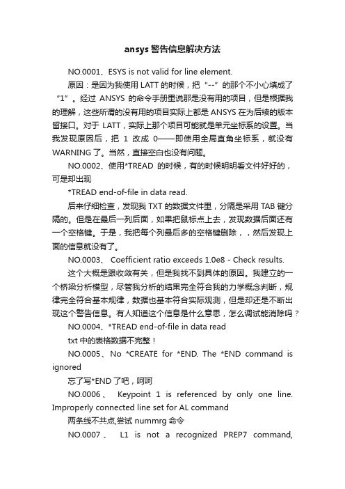
ansys警告信息解决方法NO.0001、ESYS is not valid for line element.原因：是因为我使用LATT的时候，把“--”的那个不小心填成了“1”。

经过ANSYS的命令手册里说那是没有用的项目，但是根据我的理解，这些所谓的没有用的项目实际上都是ANSYS在为后续的版本留接口。

对于LATT，实际上那个项目可能就是单元坐标系的设置。

当我发现原因后，把1改成0——即使用全局直角坐标系，就没有WARNING了。

当然，直接空白也没有问题。

NO.0002、使用*TREAD的时候，有的时候明明看文件好好的，可是却出现*TREAD end-of-file in data read.后来仔细检查，发现我TXT的数据文件里，分隔是采用TAB键分隔的。

但是在最后一列后面，如果把鼠标点上去，发现数据后面还有一个空格键。

于是，我把每个列最后多的空格键删除，，然后发现上面的信息就没有了。

NO.0003、 Coefficient ratio exceeds 1.0e8 - Check results.这个大概是跟收敛有关，但是我找不到具体的原因。

我建立的一个桥梁分析模型，尽管我分析的结果完全符合我的力学概念判断，规律完全符合基本规律，数据也基本符合实际观测，但是却还是不断出现这个警告信息。

有人知道这个信息是什么意思，怎么调试能消除吗？NO.0004、*TREAD end-of-file in data readtxt中的表格数据不完整！NO.0005、No *CREATE for *END. The *END command is ignored忘了写*END了吧，呵呵NO.0006、Keypoint 1 is referenced by only one line. Improperly connected line set for AL command两条线不共点,尝试 nummrg命令NO.0007、L1 is not a recognized PREP7 command,abbreviation, or macro.This command will be ignored 还没有进入prep7，先：/prep7NO.0008、Keypoint 2 belongs to line 4 and cannot be moved 同一位置点2已经存在了，尝试对同位置的生成新点换个编号，比如1002NO.0009、Shape testing revealed that 32 of the 640 new or modified elements violate shape warning limits.To review test results, please see the output file or issue the CHECK command.单元形状奇异，在我的模型中6面体单元的三个边长差距较大，可忽略该错误NO.0010、用命令流建模的时候遇到的The drag direction (from the keypoint on drag line 27 that is closest to a keypoint KP of the given area 95) is orthogonal to the area normal at that KP.Area cannot be dragged by the VDRAG command.意思是拉伸源面的法向与拉伸路径垂直，不能使用VDRAG命令。

违背定律英语

违背定律英语全文共四篇示例，供读者参考第一篇示例：违背定律（Violation of Law）是指违反国家法律规定，违背法律赋予公民和组织的权利和义务，破坏社会秩序和法治的行为。

在各个国家法律体系中，都存在不同的法律规定和标准，违背定律是指在这些法律规定和标准下所做出的行为。

违背定律是社会治理的重要问题，因为它会损害社会的和谐稳定，影响人民的生活和权益，甚至引发恶劣的后果。

各国都制定了严格的法律体系和监督机制，以确保公民和组织遵守法律，维护社会秩序和法治。

在英语中，违背定律通常被称为“violation of law”或“breach of law”。

违背定律的行为多种多样，包括但不限于：盗窃、偷税漏税、贪污腐败、故意伤害、违反交通规则、侵犯知识产权、违反劳动法等。

这些行为不仅损害了他人的利益，也触犯了法律，需要受到法律的制裁和处罚。

违背定律是一种违法行为，其后果往往不可预测和不可挽回。

我们每个人都应该自觉遵守法律，不做出违法行为，维护社会的和谐稳定和法治秩序。

只有通过共同努力，我们才能建设一个更加公正、文明和法治的社会。

【字数不足，需要重新增加内容】第二篇示例：违背定律，即违反法律或规定。

在现代社会中，法律是维护社会秩序和正常运作的重要保障，违背定律会导致不良后果和社会危机。

在英语中，违背定律通常用violate the law或break the law来表示。

本文将探讨违背定律在英语中的相关用法以及其重要性。

违背定律在英语中通常用violate the law或break the law来表达。

violate是动词，意为违背，违反；law是名词，意为法律。

violate the law可译为违反法律，违背定律。

在日常生活中，我们常听到类似的表达，例如：“He violated the law by speeding on the highway.”（他因在高速公路上超速而违法了。

）“Breaking the law will result in serious consequences.”（违法行为将带来严重后果。

Measure of the size of CP violation in extended models

CP violation is said to be maximal when the products Im VijVk∗jVklVi∗l acquire its maximum
absolute value. This occurs of all the matrix elements
iws h1e/n√t3hearnedistmheaxpihmausemomf iVxuidnVgc∗idnVctshVeu∗Cs KisM2πm/a3t. riNx:evtehrethmeoledsusluass
Refs. [3, 4, 5] although our deﬁnitions will be based on quantities invariant not only under
rephasings of the CKM matrix but under arbitrary quark basis transformations.
[1, 2, 3, 4, 5] since experiment [6] revealed that the phase appearing in the Cabibbo-Kobayashi-
Maskawa (CKM) matrix [7] had to be large to explain the observed CP violation in the K0K¯ 0 system. As shown by Wolfenstein [1] any deﬁnition of maximal CP violation based on
depends on the adoption of the Murnaghan construction as well as on the order in which the

Spontaneous Lorentz Violation, Gravity, and Nambu-Goldstone Modes

1 2
κ(BµBν
±
b2)2,
where
κ
is
a
constant
(of
mass
dimension
zero).
In the former case,
only excitations that stay within the potential minimum (the NG modes) are allowed by
terms and is purely an auxiliary ﬁeld. In contrast, the Lorentz NG modes do propagate.
They comprise a massless vector, with two independent transverse degrees of freedom
condition, bµAµ = 0. Hence, we conclude that spontaneous local Lorentz violation may provide an alternative explanation for massless photons. In the bumblebee model, the
arXiv:0704.2994v2 [gr-qc] 24 Apr 2008
SPONTANEOUS LORENTZ VIOLATION, GRAVITY AND NAMBU-GOLDSTONE MODES 1
Robert Bluhm Physics Department
Colby College Waterville, ME 04901 USA
photon ﬁelds couple to the current Jµ as conventional photons, but also have additional Lorentz-violating background interactions like those appearing in the Standard-Model

CP and T violation in non-perturbative chiral gauge theories

HU-EP-05/17
CP and T violation in non-perturbative chiral gauge theories
arXiv:hep-lat/0504004v1 6 Apr 2005
Werner Kerler Institut f¨ ur Physik, Humboldt-Universit¨ at, D-12489 Berlin, Germany
we get the decomposition of the Dirac operator into Weyl operators ¯+ DP− + P ¯− DP+ . D=P ¯+ in the following, we write them in the form Considering P− and P 1 l − γ 5 G ), P− = (1 2 ¯+ = 1 (1 ¯ 5 ), P l + Gγ 2 (2.3) (2.2)
Obviously the form of the chiral projections based on (1.1) represents a rather special case. Thus ﬁrstly the question arises whether the observed symmetry violations really persist in general. Secondly instead of only tracing the violations back to a parameter singularity to reveal the precise reason for them is preferable. Thirdly then to get quantitative hold of the violations is desirable. In a more general approach [8] it has been shown that the symmetric situation of contiuum theory in the CP case is not admitted due to certain operator properties. The ¯ and D there have been functions of a basic unitary operator. Though this operators G, G formulation includes all chiral operators discussed so far as special cases [9], relying on the mentioned unitary operator introduces unnecessary restrictions and forms an obstacle for a more thorough investigation of the indicated symmetries. To investigate CP, T and CPT symmetries in a general way, we here ﬁrst analyze the possible properties of the chiral projections starting from the Dirac operator and imposing only minimal conditions. We ﬁnd that due to a contribution which inevitably comes with ¯ one generally gets G ¯ = G. Furthermore, since the overall sign of opposite sign in G and G the respective contribution remains open, it becomes obvious that in the construction of the chiral projections one is confronted with two distinct possibilities, of which one must be chosen to describe physics. We next show that CP transformations as well as T transformations interchange the ¯ . This together with the fact that one generally has G ¯ = G then is seen rˆ oles of G and G to constitute the origin of the symmetry violations. With respect to the need of choosing one of the mentioned two possibilities in the construction the interchange under CP and under T transformations means to violate the original choice. On the other hand, CPT ¯ = G. symmetry is seen to be generally there and not to be aﬀected by G Finally, considering correlation functions for any value of the index, we point out that the symmetry violation eﬀects enter them via the bases involved. To get quantitative hold ¯ would be supplemented of such eﬀects we note that if the related interchange of G and G by a change of the respective sign in the construction one would get symmetry. Thus the eﬀect of the violation turns out to be given by the diﬀerence of the results for the two sign choices and is seen to become manifest in entirely diﬀerent subsets of bases contributing to the correlation functions. In Section 2 we introduce basic relations and analyze the possibilities for the chiral projections. In Section 3 we derive the properties for CP, T and CPT transformations. In Section 4 we consider the eﬀects caused in correlation functions. Section 5 contains our conclusions.

CP and T Violation in Neutrino Oscillations and Invariance of Jarlskog's Determinant to Mat

RAL-TR/1999-086 hep-ph/9912435 20 December 1999
CP and T Violation in Neutrino Oscillations and Invariance of Jarlskog’s Determinant to r Eﬀects
arXiv:hep-ph/9912435v1 21 Dec 1999
2
trix, Mν is in general, an arbitrary 3x3 matrix. The Hermitian square of the neutrino † mass matrix, Mν Mν , may be diagonalised to ﬁnd its eigenvalues, and its eigenvectors form the columns of the lepton mixing matrix, U. It is well-known that under these circumstances, neutrinos propagating in vacuum undergo ﬂavour oscillations, and furthermore, in general, these result in CP - and T -violating asymmetries. The CP - and T -violating asymmetries in the transition probabilities are given (for arbitrary mixing matrix) by the universal function P (να → νβ ) − P (ν α → νβ ) = P (να → νβ ) − P (νβ → να ) = 16J sin (∆12 L/2) sin (∆23 L/2) sin (∆31 L/2)

On the Spontaneous CP Breaking in the Higgs Sector of the Minimal Supersymmetric Standard M

b
g b Vb −
f
where gb (gf ) denotes the number of degrees of freedom of bosons (fermions). In the bosonic part we sum over stops, neutral scalar and charged Higgses, and Goldstone bosons (b = ˜L,R , h, H, H ± , G± ), and in the fermionic one we consider neutralinos and charginos (f = t χ ˜o , χ ˜± ). Working in the ’t Hooft–Landau gauge and in the DR renormalization scheme, we will decompose the bosonic components as
2 2 (2) m2 3 − λ6 v1 − λ7 v2 < 1. 4λ5 v1 v2 In the MSSM these conditions are not satisﬁed (at tree level) because in this case supersymmetry gives 1 (g 2 + g ′ 2 ), λ1 = λ2 = 8
J.R. Espinosa †, J.M. Moreno and M. Quir´ os Instituto de Estructura de la Materia, CSIC Serrano 123, E–28006 Madrid, Spain
Abstract We revise a recently proposed mechanism for spontaneous CP breaking at ﬁnite temperature in the Higgs sector of the Minimal Supersymmetric Standard Model, based on the contribution of squarks, charginos and neutralinos to the one-loop eﬀective potential. We have included plasma eﬀects for all bosons and added the contribution of neutral scalar and charged Higgses. While the former have little eﬀect, the latter provides very strong extra constraints on the parameter space and change drastically the previous results. We ﬁnd that CP can be spontaneously broken at the critical temperature of the electroweak phase transition without any ﬁne-tuning in the parameter space.

(Non-) Gibbsianness and phase transitions in random lattice spin models

a rXiv:mat h-ph/99424v126Apr1999(NON-)GIBBSIANNESS AND PHASE TRANSITIONS IN RANDOM LATTICE SPIN MODELS ∗Christof K¨u lske 1WIAS Mohrenstrasse 39D-10117Berlin,Germany Abstract:We consider disordered lattice spin models with ﬁnite volume Gibbs measures µΛ[η](dσ).Here σdenotes a lattice spin-variable and ηa lattice random variable with prod-uct distribution I P describing the disorder of the model.We ask:When will the joint measures lim Λ↑Z Z d I P (dη)µΛ[η](dσ)be [non-]Gibbsian measures on the product of spin-space and disorder-space?We obtain general criteria for both Gibbsianness and non-Gibbsianness providing an interesting link between phase transitions at a ﬁxed random conﬁguration and Gibbsianness in product space:Loosely speaking,a phase transition can lead to non-Gibbsianness,(only)if it can be observed on the spin-observable conjugate to the independent disorder variables.Our main speciﬁc example is the random ﬁeld Ising model in any dimension for which weshow almost sure-[almost sure non-]Gibbsianness for the single-[multi-]phase region.We also discuss models with disordered couplings,including spinglasses and ferromagnets,where various mechanisms are responsible for [non-]Gibbsianness.Key Words:Disordered Systems,Gibbs-measures,non-Gibbsianness,Random Field Model,Random Bond Model,SpinglassI.IntroductionThe purpose of this paper is to present a class of measures on discrete lattice spins showing a rich behavior w.r.t.their Gibbsianness properties.The examples we consider turn up in a natural context of well-studied disordered systems.Given a random lattice system,such as the randomﬁeld Ising model,we look at the joint distribution of spins and random variables describing the disorder.It is now very natural from a probabilistic point of view to consider the corresponding joint measures on the skew space resulting from the a-priori distribution of the disorder variables.Taking the inﬁnite volume limit leads to inﬁnite volume measures on the skew space.We will investigate the Gibbsianness-properties of such measures,for generalﬁnite range potentials.As we will see,this gives rise to a whole family of interesting examples of measures with non-trivial behavior.Why consider these measures?-Gibbs measures are the basic objects for a mathematically rigorous description of equilibrium statistical mechanics.They are characterized by the fact that theirﬁnite volume conditional expectations can be written in terms of an absolutely summable interaction potential.The failure of the Gibbsian property is linked to the emergence of long-range correlations or hidden phase transitions.In the theory of disordered systems on the other hand,the understanding of potentially non-local behavior as a function of the disorder variables is very important.It is a general theme that comes up very soon in any serious analysis of a lot of disordered systems. E.g.,it leads to technically involved concepts like that of a‘bad region’in space where the realization of the random variable was exceptional that must be treated carefully because it could lead to non-locality.Now,as we will see in our general investigation,the[non-]Gibbsianness of the joint measures is related in an interesting way to the[non-]locality of certain expectations of random Gibbs-measures as a function of the disorder variables.Since such a non-locality can arise in a variety of diﬀerent ways,there is a variety of diﬀerent‘mechanisms’for non-Gibbsianness.So,the much-disputed phenomenon of non-Gibbsianness becomes related in a somewhat surprising way to continuity questions of the random Gibbs measures on the spins w.r.t.disorder,or,in other words,phase transitions induced by changes of the disorder variables.The present investigation was motivated by the special recent example of the Ising-ferromagnet with site-dilution(‘GriSing randomﬁeld’)that was shown to be non-Gibbsian but almost Gibbsian in[EMSS]where an interesting realization of the disorder variables leading to‘non-continuity’was found.Mathematically the analysis was simpliﬁed here because the system considered breaks down intoﬁnite pieces.This is of course not true in most of the systems ofinterest(say:the randomﬁeld Ising model).Such a‘non-decoupling’is going to be an essential complication of the general treatment we are going to present,as we will see.Let us remark that there has been some discussion during the last years about numer-ous examples of non-Gibbsian measures,to what extent the failure of the Gibbsian property has to be taken serious,and what suitable generalizations of Gibbsianness should be(see e.g. [F],[E],[DS],[BKL],[MRM],references therin,and the basic paper[EFS]).While this discussion still does not seem to beﬁnished,the answers seem to depend on the speciﬁc situation.Our point in this context is less a general philosophical one,but to provide interesting examples that show(non-)Gibbsianness in a slightly diﬀerent light related to important issues in the theory of random Gibbs measures.More precisely we will do the following:Basic Deﬁnitions:Denote byΩ=ΩZ Z d0the space of spin-conﬁgurationsσ=(σx)x∈Z Z d,whereΩ0is aﬁniteset.Similarly we denote by H=H Z Z d0the space of disorder variablesη=(ηx)x∈Z Z dentering the model,where H0is aﬁnite set.Each copy of H0carries a measureν(dηx)and H carries the product-measure over the sites,I P=ν⊗Z d.We denote the corresponding expectation by I E. The space of joint conﬁgurationsΩ×H=(Ω0×H0)Z Z d is called skew space.It is equipped with the product topology.We consider disordered models whose formal inﬁnite volume Hamiltonian can be writtenin terms of terms of disordered potentials(ΦA)A⊂Z Z d,Hη(σ)= A⊂Z Z dΦA(σ,η)(1.1)whereΦA depends only on the spins and disorder variables in A.We assume for simplicityﬁnite range,i.e.thatΦA=0for diam A>r.A lot of disordered models can be cast into this form.Forﬁxed realization of the disorder variableηwe denote byµσb.c.Λ[η]the correspondingﬁnite volume Gibbs-measures inΛ⊂Z Z d with boundary conditionσb.c..As usual,they are the probability measures onΩthat are given by the formulaµσb.c.Λ[η](f):= σΛf(σΛσb.c.Z Z d\Λ)e−A∩Λ=∅ΦA(σΛσb.c.Z d\Λ,η)We look at spins and disorder variables at the same time and deﬁne joint spin variablesξx=(σx,ηx)∈Ω0×H0.The objects of main interest will then be the correspondingﬁnite vol-.They are the probability measures on the skew space(Ω0×H0)Z Z d ume joint measures Kσb.c.Λthat are given by the formula(F):= I P(dη) µσb.c.Λ[η](dσ)F(σ,η)(1.3)Kσb.c.Λfor any bounded measurable joint observable F:Ω×H→I R.We will consider the following examples in more detail:(i)The Random-Field Ising Model:The single spin space isΩ0={−1,1}.The Hamilto-nian isHη(σ)=−J <x,y>σxσy−h xηxσx(1.4) where the formal sum is over nearest neighbors<x,y>and J,h>0.The disorder variables are given by the randomﬁeldsηx that are i.i.d.with single-site distributionνthat is supported on aﬁnite set H0.The joint spins we will consider are given in a natural way by the Ising spin and the random ﬁeld at the same site,i.e.ξx=(σx,ηx).ξx is thus4-valued in the case of symmetric Bernoulli distribution.(ii)Ising Models with Random Couplings:Random Bond,EA-Spinglass The single spin space isΩ0={−1,1}.The Hamiltonian isHη(σ)=− x,e J x,eσxσx+e(1.5)where the formal sum is over sites x∈Z Z d and the nearest neighbor vectors in the positive lattice directions,i.e.e∈{(1,0,0,...,0),(0,1,0,...,0),...,(0,0,...,1)}=:E.The random variablesJ x,e takeﬁnitely many values,independently over the‘bonds’x,e.Speciﬁc distributions we will consider are e.g.(a)Random Bond:J x,e takes values J1,J2>0(b)EA-Spinglass:Symmetric(non-degenerate)3-valued,J x,e takes values−J,0,J withν(J x,e=J)=ν(J x,e=−J),0<ν(J x,e=0)<1We deﬁne the joint spins by the Ising spin and the collection of adjacent couplings pointing in the positive direction,i.e.ξx=(σx,ηx)=(σx,(J x,e)e∈E).It is thus16-valued in dimension3in case(a).We think of the Random Field Ising model for a moment to motivate what we are going to do.Recall that,in two dimensions,for almost every realization of the random ﬁelds ηw.r.t.to the I P there exists a unique inﬁnite volume Gibbs measure µ(η)(see [AW]).In three or more dimensions,for low temperatures and ‘small disorder’there exist ferromagnetically ordered phases µ+,−(η)obtained by diﬀerent boundary conditions [BK].Diﬀerent from the GriSing example of [EMSS]we can hence consider various inﬁnite volume versions of the form ‘I P (dη)µ(η)(dσ)’.The most general thing now that we can reasonably do,is to ﬁx any boundary condition σb.c..Then,due to compactness,there are always subsequences such that the corresponding K σb.c.Λ(dξ)converges weakly to a probability measure on the skew space that we call K (dξ).Note that this measure can in general depend on the boundary condition and the particular choice of the subsequence in d ≥2.It can be shown that:by conditioning K (dξ)=K (dσ,dη)on the disorder variable ηone obtains a (not necessarily extremal)random inﬁnite volume Gibbs-measure,for I P -almost every η.1The aim of this paper is to investigate the question:When are the weak limit points of K σb.c.Λ(dξ)Gibbs-measures on the skew-space?When are they almost [almost not]Gibbs?This investigation is about continuity properties of conditional expectations.Throughout the paper we will use the following notion of continuity that involves only uniquely deﬁned ﬁnite volume events.Following [MRM]we say:Deﬁnition:A point ξ∈Ω×H is called good conﬁguration for K ,if sup ξ+,ξ−Λ:Λ⊃V K (˜ξx ξV \x ,ξ+Λ\V )−K (˜ξx ξV \x ,ξ−Λ\V ) →0(1.6)with V ↑Z Z d ,for any site x ∈Z Z d ,for any ˜ξx ∈H 0.Call ξbad ,if it is not good.As usual we have written ξA =(ξx )x ∈A (and will also do so for σA ,ηA ).In words:Good conﬁguration are the points ξwhere:The family of conditional expectations of K is equicontinuous w.r.t.the parameter Λ.We recall:If there are no bad conﬁgurations,the measure K is Gibbsian (see [MRM]).If Gibbsianness does not hold,one can ask for the K -measure of the set of bad conﬁgurations.We say that K is almost Gibbsian,if it has K -measure zero.If it has K -measure one,we say that K is almost non-Gibbsian.(See also the beginning of the next chapter.)In the remainder of the paper we will prove criteria that ensure that a conﬁguration(η,σ)is good or bad(see propositions1-6).It might not be very intuitive atﬁrst sight to understand why such measures can ever be non-Gibbsian.Let us stress the following facts:Surely,the conditional expectation of the spin-variableσx given the joint variableξ=(σ,η)away from x andηx is a local function,given by the local speciﬁcations.Trivially,the conditional expectation of the disorder variableηx givenηaway from x is a local function-it is even independent.However: The conditional expectation ofηx givenηandσaway from x can be highly nontrivial,due to the coupling between spins and disorder arising from the local speciﬁcations(1.2).Rather than presenting our general results at this point,we specialize to the Random Field Ising Model.For this model there is a complete characterization of a bad conﬁguration in terms of the behavior of theﬁnite volume Gibbs-measures that is particularly transparent.We obtain:Theorem1:Consider a randomﬁeld Ising model of the form(1.4),in any dimension d.A conﬁgurationξ=(η,σ)is a bad conﬁguration for any joint measure obtained as a limit point of theﬁnite volume joint measures I P(dη)µσb.c.∂ΛΛ[η]if and only iflim Λ↑∞µ+Λ[ηΛ](˜σx=1)>limΛ↑∞µ−Λ[ηΛ](˜σx=1)(1.7)for some site x,independent ofσ.Hereµ+,−Λare theﬁnite volume Gibbs measures with+(resp.−)boundary conditions.Note,that the theorem will hold for the joint measures corresponding to Dobrushin states that are supposed to exist in d≥4.1Using the known results about the randomﬁeld model one immediately obtains:Corollary:(i)d=1:K is Gibbsian,for all J,h>0.(ii)d=2:K is a.s.Gibbsian for all J,h>0.On the other hand,suppose thatν[ηx=0]>0.Assume that J is suﬃciently large andh>0.Then K is not Gibbsian.(iii)d≥3,νsymmetric,J>0suﬃciently large,ν[η2x]suﬃciently small.Then any such K isa.s.not Gibbs.Indeed:The a.s.Gibbsianness in d=2follows from the a.s.absence of ferromagnetism, proved in[AW].That we have Non-Gibbsianness in d≥2if the support of the randomﬁelds contains zero follows from the fact that the conﬁgurationξ=(ηx≡0,σ)is a bad,if J islarge enough s.t.there is ferromagnetic order in the homogeneous Ising ferromagnet.A.s.non-Gibbsianness under the conditions(iii)follows from the existence ferromagnetic order,proved in[BK].The organization of the paper is as follows.In Chapter II we investigate the one-site conditional probabilities of K and prove general criteria that ensure that a conﬁguration is good or bad.We will see that the important general step is to consider the single-site variation of the Hamiltonian w.r.t.the disorder variableηx and rewrite the conditional expectations in the form of Lemma1.This leads to expressions involving certain expectations of the‘conjugate’spin-observable.In the example of the randomﬁeld model this observable is just the spinσx;thus the corresponding criteria in Theorem(i)are simply formulated in terms of the magnetization.In Chapter III we apply our results.We prove Theorem1about the RFIM.Next we comment on Models with decoupling conﬁgurations,recalling the GriSing randomﬁeld of[EMSS] and Models with random couplings(including spinglasses)that can be zero.This provides more examples of non-Gibbsianﬁelds.Next we specialize our criteria of Chapter II to Models with random couplings,proving Theorem2.Based on this we give a heuristic discussion explaining how the validity of the Gibbsian property can be linked to the absence of random Dobrushin states.Acknowledgments:The author thanks A.van Enter for a private explanation of reference[EMSS].II.Criteria for joint[non-]GibbsiannessIn this chapter we are going to investigate whether a conﬁgurationξ=(η,σ)is good or bad for the joint states K.We will obtain criteria that are given in terms of the local speciﬁcations. To do so we introduce the single-site variation of the Hamiltonian w.r.t.disorder(2.2)and use theﬁnite volume perturbation formula(2.3)to rewrite the conditional expectations of K in the form of Lemma1.This leads to the characterization of good resp.bad conﬁgurations of the Corollary of Proposition1.As direct consequences thereof,Propositions2and3give more convenient conditions that ensure goodness resp.badness.Under the additional assumption of a.s.convergent Gibbs measures we obtain the slightly less obvious criterion for badness of Proposition4.Before we start,let us however summarize the following facts about the notion of good conﬁguration and its relevance for Gibbsianness,for the sake of clarity:(i)Ifξis bad for K any version of the conditional expectationξZ Z d→K(ξx|ξZ Z d\x)must bediscontinuous for some site x(use DLR-equation,see Proposition4.3[MRM]).(ii)Conversely:Assume thatˆξ∈G:={ξ;ξis good}.Then limΛ↑Z Z d K(ξx|ˆξΛ\x)exists for any site x and hence also limΛ↑Z Z d K(ξV|ˆξΛ\V)=:γV(ξV|ˆξZ Z d\V)exists for anyﬁnite volume V.If G has full measure w.r.t K,the above limit can be(arbitrarily)extended to a measur-able function of the conditioning.It is readily seen to deﬁne a version of the conditional expectationξZ Z d\V→K(ξV|ξZ Z d\V)that is continuous within the set G[i.e.:ξ(N)→ξwith ξ(N),ξ∈G implies K(ξV|ξ(N)Z Z d\V)→K(ξV|ξZ Z d\V)].(See[MRM]:Proof of Proposition4.4).In this situation we call K almost Gibbs.1In particular:If every conﬁguration is good,the measure K has a version of the conditional expectation that is continuous on the whole space and is Gibbs therefor.In the sequel it will be important to keep track of the local dependence of various quantities.It will be useful to make this explicit.We use the followingNotation:For theﬁxed interaction range r we introduce the r-boundary∂B={x∈Z Z d\B;d(x,B)≤r}.In the same fashion we writeΛ)=I PΛ)µσb.c.∂ΛΛ[ΛN\Λµσb.c.∂ΛNΛN[ηx,ηΛ\x,˜ησ′x I EΛN\Λ](σ′x,σΛ\x)=µσ∂x x[ηx,η∂x](σx)(2.1)where the second equality follows from the application of the compatibility relation for theµ-measures for the inner volume made of the single site x,as soon asΛ⊃1If K(G)=1but G=H×Ω,we have:G is dense in H×Ω[since any ball w.r.t.a metric for the product topology has to have positive K-mass,under the assumption of bounded interactions Φ.]Thus the conditional expectation is continuous on G but necessarily not uniformly continuous (because it could be extended to the whole space otherwise.)non-locality as a function of σΛ\x ,ηΛ\x in this term.On the other hand we see that,if the conditional ηx -distribution has a non-local behavior as a function of σΛ\x ,ηΛ\x ,this carries over also to the σx -marginal K σb.c.∂ΛN ΛN σx σΛ\x ;ηΛ\x = K σb.c.∂ΛN ΛN d ˜ηx σΛ\x ;ηΛ\x µσ∂x x [˜ηx ,η∂x ](σx )unless the dependence on ˜ηx of the one-site expecta-tion under the last integral is trivial,of course.After these simple remarks we come to the important formula that is going to be the starting point of all our analysis.Let us deﬁne the single-site-variation of the Hamiltonian w.r.t.the disorder variable 1ηx at the site x to be∆H x (σx ,ηx η∂x )−ΦA σΛ\x ](dσΛ)f (σΛ)= µσb.c.∂ΛΛ[η0x ,ηx ,ηx ,η0x ,η∂x )Λ\x ](dσΛ)e −∆H x (σΛN \Λ σ∂−Λ;η0x ,ηΛ\x µσb.c.∂ΛN ΛN [η0x ,ηΛ\x ,˜ηx )e−∆H x (˜σΛN \Λ σ∂−Λ;η0x ,ηΛ\x µσb.c.∂ΛN ΛN [η0x ,ηΛ\x ,˜ηx )e−∆H x (˜σ1A quantity of this type also plays a crucial role in [AW]where the ﬂuctuations of extensive quantities are investigated.Its Gibbs expectation could be termed ‘order parameter that is conju-gate to the disorder’.Proof:To compute the conditional distribution of ηx we use the ﬁnite volume perturbation formula to extract the variation of ηx .We use a convention to put tildes on quantities that are integrated and writeK σb.c.∂ΛN ΛN σΛ\x ;ηx ,ηΛ\x =I P (ηx )I P (ηΛ\x )×I EΛN \Λ](σΛ\x )=I P (ηx )I P (ηΛ\x )×I EΛN \Λ](d ˜σΛ)e −∆H x (˜σ µσb.c.∂ΛN ΛN [η0x ,ηΛ\x ,˜ηx ,ηx ,η0x ,η∂x )=I P (ηx )×I P (ηΛ\x )µσ∂−ΛΛo [η0x ,ηΛ\x ](σΛo \x )× µσ∂x x [η0x ,η∂x](d ˜σx )e −∆H x (σ∂x ,˜σx ,ηx ,η0x ,η∂x )×I E ΛN \Λ](σ∂−Λ)ΛN \Λ](d ˜σΛ)e −∆H x (˜σΛN \Λµσb.c.∂ΛN ΛN [η0x ,ηΛ\x ,˜η µσb.c.∂ΛN ΛN [η0x ,ηΛ\x ,˜ηx ,ηx ,η0x ,η∂x )= K σb.c.∂ΛN ΛN d ˜ηΛN \Λ](d ˜σx ,ηx ,η0x ,η∂x ) −1×I EΛN \Λ](σ∂−Λ)(2.6)where the term in the last line is just a constant for ηx .♦Remark:The formula gives the modiﬁcation of the conditional expectation compared with the ‘free’a-priori measure ν(ηx )that results from the non-trivial coupling of ηto the spin-variable σ.The second term in the second line of (2.4),a Gibbs expectation of the exponential of the single-site variation of the Hamiltonian,is of course a local function in the conditioning.Assuming the ﬁniteness of the potential it is bounded.Thus,to investigate the potential non-locality of the l.h.s.one has to investigate the third line of (2.4).Remark:The local ΛN -limit of the conditional expectation K σb.c.∂ΛN ΛN d ˜ηthe existence of aΛN-limit on the l.h.s.of(2.5).TheΛN limit of the last line of(2.6)[the normalization needed to obtain probabilities]also exists by the hypothesis.Sometimes it is convenient to rewrite(2.4)using that,by theﬁnite volume perturbation formula,we haveµσb.c.∂ΛNΛN[η0x,ηΛ\x,˜ηx)e−∆H x(˜σΛN\Λ](d˜σx,ηx,η0x,η∂x)≡µσb.c.∂ΛNΛN[ηΛ,˜ηΛN\Λ]/Zσb.c.∂ΛNΛN[ηxηΛ\x˜ηK η2x σΛ\x;ηΛ\x =q local(η1x,η2x,σ∂x,η∂x)q nonlocΛ,x[η1x,η2x,ηΛ\x,σ∂−Λ](2.8) whereq local(η1x,η2x,σ∂x,η∂x)=ν(η1x)ΛN\Λ σ∂−Λ;η2x,ηΛ\xµσb.c.∂ΛNΛN[η1x,ηΛ\x,˜ηx)e∆H x(˜σend that both q ’s in Proposition 0are uniformly bounded against zero and one,by the assumed ﬁniteness of ∆H x .♦To understand the symmetry between η1and η2in this formula we remark that q local as well as the inner integral in (2.10)can be written as fractions of partitions functions,by the remark following (2.7).We will now discuss various consequences of Corollary of Proposition 1.It is very diﬃcult to say anything reasonable about the behavior of the conditional measure K σb.c.∂ΛN ΛN d ˜ηΛ\V] e ∆H x (η1x ,η2x ,η∂x ) −µσb.c.∂ΛΛ[η1x ,ηV \x ,η−ΛN \Λ] e∆H x (η1x ,η2x ,η∂x )−µσb.c.∂ΛN ΛN[η1x ,ηx ,η1x ,η2x ,η∂x )≤r V,x (η1x ,η2x ,η)(2.13)to compare the µ-terms under the ˜η-integrals with a term that is independent of ˜ηand η+,−.This shows that (2.11)is bounded by 2r V,x which converges to zero.♦Remark:To estimate r V,x (η1x ,η2x ,η)we can also bound the variation of the random cou-plings by the variation over the boundary conditionsr V,x (η1x ,η2x ,η)≤sup σ1,σ2µσ1∂−V V o [η1x ηV \x ] e ∆H x (η1x ,η2x ,η∂x ) −µσ2∂−V V o [η1x ηV \x ] e ∆H x (η1x ,η2x ,η∂x )(2.14)Remark:We see,how(2.12)parallels(1.6).The quantity that is of interest is now the Gibbs-expectation of the exponential of the single-site variation as a function of the disorder variables.In words:If we have equicontinuity in the parameterΛof theseﬁniteΛ-Gibbs expec-tations w.r.t.the disorder variable at the pointη,we conclude thatη,σis a good conﬁguration. The reader may alsoﬁnd it intuitive to rewrite the Gibbs-expectations appearing in(2.12)in the form of fractions of partition functions,or(equivalently)as exponentials of diﬀerences of free energies taken forη1x andη2x.In slightly diﬀerent words the criterion thus requires:Equiconti-nuity in the volume of the single site-variations of the free energies w.r.t.the disorder variable at the pointη.To get a criterion for bad conﬁgurations that is independent of the behavior of the outer expectation of q nonloc[see(2.10)]leads to an expression that is slightly more complicated because it contains an additional supremum.Proposition3:Putq upper Λ,x [η1x,η2x,ηΛ\x]:=lim supΛN↑Z Z dsup˜ηΛN\Λ] e∆H x(η1x,η2x,η∂x) (2.15)Thenη,σis a bad conﬁguration for K,if for some site x,for some pairη1x,η2xlim V↑Z Z dsupη+,η−Λ:Λ⊃Vq upperΛ,x[η2x,η1x,ηV\x,η+Λ\V] −1−q upperΛ,x[η1x,η2x,ηV\x,η−Λ\V] >0(2.16)Proof:By(2.7)and the uniform estimate of the˜η-integral we see that thatq nonloc Λ,x [η1x,η2x,ηΛ\x,σ∂−Λ]≤q upperΛ,x[η1x,η2x,ηΛ\x],≥q upperΛ,x[η2x,η1x,ηΛ\x]−1(2.17)Hence the claim(discontinuity of the l.h.s.)follows from the deﬁnition of a bad conﬁguration.♦Models with a.s.convergent Gibbs states:Suppose that we have the existence of a weak limitlim Λ↑Z Z d µσb.c.∂ΛΛ[ηΛ]=µ∞[ηZ Z d](2.18)for I P-a.e.η.It follows thatµ∞[ηZ Z d]is an inﬁnite volume Gibbs measure for P-a.e.ηthat depends measurably onη.Consequently the inﬁnite volume joint state is then just the I P-integralofµ∞.We stress that this has not been assumed so far and is really a much stronger assumption then local convergence of the joint states.It is not expected to hold e.g.for spinglasses in the multi-phase region(that is supposed although not proved to exist).This assumption implies that the terms in the main formula of Lemma1converge individ-ually withΛN↑Z Z d.So we have thatq nonloc Λ,x [η1x,η2x,ηΛ\x,σ∂−Λ]= K d˜ηZ Z d\Λ σ∂−Λ;η2x,ηΛ\x µ∞[η1x,ηΛ\x,˜ηZ Z d\Λ] e∆H x(η1x,η2x,η∂x) (2.19) Suppose we want to exhibit a bad conﬁguration and we have estimates on the continuity ofη→µ∞[η]for typical directions but not in all directions.For an example of a perturbation in an atypical direction think of the randomﬁeld Ising model that will be discussed below.Here the Gibbs-measure with plus boundary conditions can be pushed in the‘wrong phase’by choosing the randomﬁelds to be minus in a large annulus.While the RFIM can be treated by Proposition3there are examples where we would like to get away from uniform estimates w.r.t.˜ηin favorof estimates that are only true for typical˜η,for the a-priori measure I P.To obtain the following criterion is more subtle than what we noted in Proposition2and3. The trick is to show the existence of suitable‘bad’σ-conditionings using the knowledge about typical disorder variables w.r.t.the unbiased I P-measure.Proposition4:Assume the a.s.existence of the weak limits ofﬁnite volume Gibbs measures (2.18)and denote by K the corresponding inﬁnite volume joint measure.The conﬁgurationξ=(η,σ)is a bad conﬁguration for K if:for each cube V,centered at the origin,there exists an increasing choice of volumesΛ(V),and conﬁgurationsηV,¯ηV s.t.forI P-a.e.˜ηwe have thatlim infV↑Z Z dµ∞[η1x,ηV\x¯ηVΛ(V)\V,˜ηZ Z d\Λ] e∆H x(η1x,η2x,η∂x)>lim supV↑Z Z dµ∞[η1x,ηV\xηVΛ(V)\V,˜ηZ Z d\Λ] e∆H x(η1x,η2x,η∂x) (2.20) for some site x,and someη1x,η2x.Proof:We will show that there exist two conditionings¯σandσ,s.t.lim inf V↑Z Z d q nonlocΛ(V),x[η1x,η2x,ηV\x¯ηVΛ(V)\V,¯σ∂−Λ(V)]>lim supV↑Z Z d q nonlocΛ(V),x[η1x,η2x,ηV\xηVΛ(V)\V,σ∂−Λ(V)](2.21)From this and the Corollary of Proposition1follows the badness.To show(2.21)we proceed as follows:The l.h.s.and r.h.s.of(2.20)are tail measur-able,hence a.s.constant.Denote the l.h.s of(2.20)by¯q∞[η1x,η2x,ηZ Z d\x]and the r.h.s.by q∞[η1x,η2x,ηZ Z d\x].We will show that there exists a conditioningσs.t.the r.h.s.of(2.21)is bounded from above by q∞[η1x,η2x,ηZ Z d\x].(Similarly,there exists a conditioning¯σs.t.the l.h.s. of(2.21)is bounded from below by¯q∞[η1x,η2x,ηZ Z d\x].)We will construct this conditioning as a sequence given on the‘small’annuli∂−Λ(V)(and arbitrary for other lattice sites.)To make use of the a.s.statement w.r.t the product measure I P we need to produce a formula that recovers this measure.We writelim sup V↑∞ ˜σ∂−Λ(V) K∞ ˜σ∂−Λ(V) η2x,ηV\xηVΛ(V)\V q nonlocΛ(V),x[η1x,η2x,ηV\xηVΛ(V)\V,˜σ∂−Λ(V)]=lim supV↑∞ I P(d˜η)µ∞[η1x,ηV\xηVΛ(V)\V,˜ηZ Z d\Λ] e∆H x(η1x,η2x,η∂x) ≤q∞[η1x,η2x,ηZ Z d\x](2.22)where theﬁrst equality follows from(2.19)and the inequality from Fatou’s Lemma w.r.t product-integration of the˜η.From this,the existence of such a conditioningσis easy to see.(By contradiction:If the claim were not true,for any sequence of conditioningsσ∂−Λ(V),we wouldhave that there exists a positiveǫs.t.min˜σ∂−Λ(V)q nonlocΛ(V),x[...,˜σ∂−Λ(V)]≥q∞[...]+ǫfor inﬁnitelymany V’s.But this would imply that also the quantity under the limsup on the l.h.s.of(2.22) [which is just a˜σ∂−Λ(V)-expectation]would have to be bigger of equal to this bound,for the same inﬁnitely many V’s.)♦III.ExamplesIII.1:The randomﬁeld Ising modelNote that the single site perturbation w.r.t the randomﬁeld of the Hamiltonian is very simple,i.e.e∆H x(σx,η1x,η2x)=e h(η2x−η1x)σx=e h(η1x−η2x)+2sinh h(η2x−η1x)1σx =1(3.1)An application of Propositions2and3gives,with the aid of monotonicity arguments Theorem1, as stated in the introduction.It provides a complete characterization of good/bad conﬁgurations in terms of the behavior of theﬁnite volume Gibbs-expectations with plus resp.minus boundary conditions.The interesting part,the mechanism of non-continuity,is due to the fact that we can make the randomﬁeld Gibbs measure look like the plus(minus)phase around a given site by choosing theﬁelds in a suﬃciently large annulus to be plus(minus).That this works independently of what theﬁelds even further outside do,is crucial for the argument.Proof of Theorem1:We use the fact that the function(η,σbc)→µσbcΛ[ηΛ](˜σx=1)is monotone(w.r.t.the partial order of its arguments obtained by site-wise comparison.)From。

CP Violation

On leave of absence from Departament de F´ ısica Te` orica, Universitat de Val` encia, and IFIC, Centre Mixte Universitat de Val` encia–CSIC, E-46100 Burjassot, Val` encia, Spain. † Work supported in part by CICYT (Spain), under grant No. AEN93-0234.
CERN-TH.7114/93
CP VIOLATION
arXiv:hep-ph/9312297v1 16 Dec 1993
A. Pich∗† Theory Division, CERN, CH-1211 Geneva 23
ABSTRACT An overview of the phenomenology of CP violation is presented. The Standard Model mechanism of CP violation and its main experimental tests, both in the kaon and bottom systems, are discussed.
CERN-TH.7114/93 December 1993
CP VIOLATION
A. PICH∗† Theory Division, CERN, CH-1211 Geneva 23
ABSTRACT An overview of the phenomenology of CP violation is presented. The Standard Model mechanism of CP violation and its main experimental tests, both in the kaon and bottom systems, are discussed.

Resonant CP Violation due to Heavy Neutrinos at the LHC

School of Physics and Astronomy, University of Manchester, Manchester M13 9PL, United Kingdom b Center for Theoretical Physics, School of Physics, Seoul National University, Seoul, 151-722, Korea
Abstract
The observed light neutrinos may be related to the existence of new heavy neutrinos in the spectrum of the SM. If a pair of heavy neutrinos has nearly degenerate masses, then CP violation from the interference between tree-level and self-energy graphs can be resonantly enhanced. We explore the possibility of observing CP asymmetries due to this mechanism at the LHC. We consider a pair of heavy neutrinos N1,2 with masses ranging from 100 − 500 GeV and a mass-splitting ∆mN = mN2 − mN1 comparable to their widths ΓN1,2 . We ﬁnd that for ∆mN ∼ ΓN1,2 , the resulting CP asymmetries can be very large or even maximal and therefore, could potentially be observed at the LHC.

Solution of the strong CP problem

a r X i v :h e p -p h /9611266v 1 7 N o v 1996Solution of the strong CP problemvouraUniversidade T´e cnica de LisboaCFIF,Instituto Superior T´e cnico,Edif´ıcio Ciˆe ncia (f´ısica)P-1096Lisboa Codex,Portugal February 1,2008Abstract I put forward an SU(2)L ⊗SU(2)R ⊗U(1)model in which spontaneously broken parity symmetry makes it that strong CP violation only arises at three-loop level.All leptons and up-type quarks are in doublets either of SU(2)L or of SU(2)R ,but there are singlet down-type quarks.A bi-doublet of scalars is introduced which has only one component with non-vanishing expectation value,thereby avoiding W L -W R mixing.The scalar potential is such that scalar-pseudoscalar mixing does not occur either.1Introduction Non-perturbative eﬀects in Quantum Chromodynamics (QCD)may lead to P and CP violation,characterized by a parameter θ,in hadronic processes.The experimental upper bound on the electric dipole moment of the neutron constrains θto be less than 10−9or so.The presence of this unnaturally small number in QCD is what is known as the strong CP problem.θis the sum of two terms,θQCD and θQF D .θQCD is the original value of the angle θcharacterizing the QCD vacuum.θQF D originates in the chiral rotation of the quark ﬁelds needed to render the quark masses real and positive.If M p and M n are the mass matrices of the up-type and down-type quarks,then θQF D =arg det(M p M n ).There are two general ways of solving the strong CP problem.In the ﬁrst approach it is claimed that θhas no signiﬁcance or physical consequences;theories with diﬀerent values of θare equivalent,and therefore we may set θ=0without loss of generality.This may be so because of the presence in the theory of a Peccei–Quinn symmetry [1],but there are also claims that QCD dynamics itself cures the strong CP problem [2].The second path,which I shall follow,tries to ﬁnd some symmetry which naturally leads to the smallness of θ.As θis both CP-and P-violating,we ﬁrst assume the Lagrangian (or at least its quartic part)to be either CP-or P-symmetric,thereby automatically obtaining θQCD =0.CP or P symmetry must then be either softly or spontaneously broken.While doing this the problem of ensuring the smallness ofθQF D remains.This is quitediﬃcult when using CP symmetry.After CP is broken softly or spontaneously,it is diﬃcult to avoid one-loop contributions toθQF D from the quark self-energies[3],because each neutral spin-0particle will usually have both scalar and pseudoscalarinteractions with each quark.Georgi[4]realized this,and claimed thatθQF D thus generated would be of order10−8.However,in order to make this estimate heassumed all quarks to have masses at most of order10GeV.Once it is known that the top mass is much larger than this,a suppression factor is lost,and a morelikely estimate isθQF D∼10−5,which is unacceptable.Most models using CP to suppressθ[5]suﬀer from this problem in one way or another.A remarkable exception is the model of Bento and collaborators[6].In1990theﬁrst model appeared[7]which used P symmetry to suppressθ.The general features that models of this kind have to satisfy were later analysed by Barr and collaborators[8].They claimed that a model which uses parity to suppressθmust have both mirror quarks and a duplication of the standard-model (SM)SU(2)gauge group.In their own words:“The mirror families must have diﬀerent weak interactions from the ordinary V−A ones.There is simply no escape from this conclusion;one has to double both the electroweak group and the fermionic content”.In this paper I construct a model in which the SU(2)gauge group is indeeddoubled,but the lepton and up-type-quark content is the same as in the SM, while the down-type quarks are doubled.In my modelθQF D only arises at three-loop level.The model is somehow intermediate between the standard left-right-symmetric model[9]and the models with mirror quarks[7,8],but it has some odd features,as I shall point out.2The model2.1Scalar potentialThe gauge group of the model is SU(2)L⊗SU(2)R⊗U(1).The scalar sector con-sists of a bi-doubletφ(with˜φ≡τ2φ∗τ2),a doubletχL of SU(2)L,and a doublet χR of SU(2)R.The Lagrangian is assumed to be symmetric under parity,which transformsφintoφ†and interchangesχL withχR.The gauge coupling constant of SU(2)L is equal to the one of SU(2)R,and I call it g.The electric charge is Q=T L3+T R3+Y.Up to this point,the model is similar to the usual left-right-symmetric one[9].I assume the Lagrangian to be symmetric under a discrete symmetry S,which transformsφ→iφ,χL→−χL,χR→iχR.(1)As a consequence,the scalar potential isV=µ1(χ†LχL+χ†RχR)+µ2tr(φ†φ)+m(χ†LφχR+χ†Rφ†χL)+λ1[(χ†LχL)2+(χ†RχR)2]+λ2(χ†LχL)(χ†RχR)+λ3[tr(φ†φ)]2+λ4tr(φ†˜φ)tr(˜φ†φ)+λ5{[tr(φ†˜φ)]2+[tr(˜φ†φ)]2}+λ6(χ†LχL+χ†RχR)tr(φ†φ)+λ7(χ†Lφφ†χL+χ†Rφ†φχR)+λ8(χ†L˜φ˜φ†χL+χ†R˜φ†˜φχR).(2) It is important to notice that,even though I do not impose CP symmetry,all the coupling constants in this S-and parity-symmetric potential are real.I decompose the scalar multiplets as(A may be L or R)φ= φ0∗2φ+1−φ−2φ01 ,˜φ= φ0∗1φ+2−φ−1φ02,χA= χ+Aχ0A .(3)In principle,all four neutral complexﬁelds in these multiplets may acquire a vacuum expectation value(vev).I shall however assume the vev ofφ02to vanish. That is,I assumeφ = 000k1 , ˜φ = k∗1000 , χA = 0v A .(4)This is a crucial feature of the model.The purpose of this is to avoid W L-W R mixing which,together with the diﬀerent mixing matrices for left-and right-handed currents if φ02 were non-vanishing,would lead to the generation ofθQF D at one-loop level.It is important to notice that φ02 =0is a consistent assumption since no vev forφ02is induced by the vevs ofφ01,χ0L andχ0R.This means that, when we substitute all scalarﬁelds butφ02by their vevs,no term remains in the potential which is linear inφ02.I must add the remark that the potential in eq.2 is the most general one which has parity symmetry and admits φ02 =0.Because of the gauge symmetry,the only meaningful phase in eq.4isα≡arg(v L v∗R k∗1).The value ofαisﬁxed by the only term in the potential in eq.2 which“sees”it,the term in m.However,m is real,and therefore(assuming, without loss of generality,m to be negative)αwill be zero.As there is only one term in the potential which“sees”the vacuum phase α,there is no scalar-pseudoscalar mixing.This is another crucial feature of the model.It prevents one-loop self-energy diagrams with neutral spin-0ﬁelds from generatingθQF D,which would then be too large.The absence of scalar-pseudoscalar mixing can be explicitly checked by de-veloping the potential in eq.2toﬁnd the masses of the various spin-0particles. Without loss of generality I set k1,v L and v R real and positive.I then writeφ01=k1+ρ1+iη12,φ02=ρ2+iη22,χ0A=v A+ρA+iηA2.(5)There is one massive neutral pseudoscalar,I≡(k1v RηL−k1v LηR−v L v Rη1)/N, where N≡proportional to m ,as would be expected,because if m vanished there would be another spontaneously broken U(1)symmetry (given by χL →exp(iψ)χL and χR →exp(−iψ)χR )in the potential,and then I would be a Goldstone boson.There are three massive neutral scalars,which are orthogonal combinations of ρ1,ρL and ρR .These orthogonal combinations depend on the speciﬁc values of the parameters in the potential.There are two other neutral spin-0particles,ρ2and η2.The masses of ρ2and η2are diﬀerent because of the λ5term in the potential.Finally,the physical charged scalars are H +L =(−k 1χ+L +v L φ+1)/V Land H +R =(−k 1χ+R −v R φ+2)/V R ,where V A ≡2and the mass of W R is (gV R )/√2cos θW ),and its interactions are approximately givenby (g/cos θW )(T L 3−Q sin 2θW ),with a suitably deﬁned angle θW .The above approximations are up to terms of order v L /v R or k 1/v R .This means that the lightest neutral gauge boson can be identiﬁed with the Z particle observed at LEP and SLAC if v R ≫v L ,k 1.Notice however that we do not impose any condition on k 1/v L .2.3Yukawa interactionsThe quark sector of the model consists of doublets q L of SU(2)L ,doublets q R of SU(2)R ,and left-handed N L and right-handed n R which are singlets both of SU(2)L and of SU(2)R and have electric charge −1/3.There are three (for three generations)of each of these types of quark multiplets.I writeq L = p Ln L ,q R = p RN R .(6)Parity interchanges q L with q R and N L with n R .The discrete symmetry S trans-forms q L →q L ,q R →iq R ,N L →N L ,n R →−n R .(7)As a consequence,the Yukawa Lagrangian for the quarks isL Y =−q R ˜φ†∆q L −(q R χR GN L +H.c.),(8)where∆is hermitian,while G is a general3×3complex matrix.The mass terms will then beL Y=...−(\L⊑L G\R+√u LγµγL V d L+W+RµV L k1M u VγL+k1V R k1M u VγR+k1√DV†M u VγL d+√DV†M u VγL d−The Yukawa interactions of the quarks with I and with the scalars are given by L Y=...−iI2N v L v R uM uγ5u+k1v R dM dγ5d+k1√DM d D.(14)√uM u u−ρL2vLRemember thatρ1,ρL andρR are not eigenstates of mass,rather they are related by an orthogonal transformation to the three physical scalarﬁelds.The lepton sector of the model may be chosen to be the usual one[9],without lepton singlets.This is a considerable simpliﬁcation relative to previous models which used parity to suppressθQF D[7,8].Because the vev ofφ02vanishes,the neutrino masses vanish too.In this way we do not have to explain their small value,which is a usually a problem in left-right-symmetric models.2.4CP violationIn this model CP violation is hard and manifests itself only in the complexity of the CKM matrix V.At lowest order in V,rephasing-invariant imaginary parts appear in the“quartets”Vαi Vβj V∗αj V∗βi(α=βand i=j).As is well-known [10],the imaginary parts of all quartets are equal in modulus to a value J.The experimental data on V imply that J is at most10−4.Let us consider the generation ofθQF D from the quark self-energies.Just as in the SM[11],complex self-energies arise at lowest order when they are proportional to quartets.This happens when the respective diagrams have four vertices with either the gauge bosons W or the charged spin-0particles H L or H R.This means that complex self-energies only arise at two-loop level.In the unitary gauge,the self-energies with gauge bosons W do not contribute to the masses—they are proportional to either pγL or pγR.In other gauges though,the Goldstone bosons absorbed in the longitudinal components of the W contribute an imaginary part to the mass of each quark.However,when divided by the mass of the quark and summed over allﬂavours,those imaginary parts cancel out.As a consequence the contribution toθQF D vanishes in any ing a similar argument,we can easily show that the two-loop diagrams involving the spin-0chargedﬁelds H L and H R do not contribute toθQF D either.Therefore,strong CP violation only arises at three-loop level.This is the same as happens in the SM[11].θwill be suppressed by the factors J<∼10−4and (16π2)−3∼10−6.Therefore,we expectθto be no larger than10−10.However,as was pointed out in the analysis of Ellis and Gaillard[11],factors m q/m W should be present too,where m q are second-generation quark mases.These factors m q/m W further suppressθQF D to values of order10−16.Moreover,in models which use parity symmetry to obtainθQF D=0at tree level,there must be extra suppression factors at loop level arising from a partial cancellation between the contributions toθQF D from the usual quarks and from the mirror sector[8].Therefore,10−16 is only an upper bound forθQF D,which in the present model is probably much smaller than that.3ConclusionsIt is important to stress the diﬀerences between the present model and previousones[7,8]which used parity symmetry to suppressθQF D.This model has less fermions,because it avoids doubling the lepton spectrum and the up-type-quark spectrum.On the other hand,it has more spin-0ﬁelds,because of the use of a bi-doublet of SU(2)L and SU(2)R.The presence of adiscrete symmetry is crucial to obtain φ02 =0;this in turn is important because it allows us to have vanishing neutrino masses.The asymmetry between up-typeand down-type quarks,with twice as many charge−1/3quarks as charge2/3 quarks,is an interesting feature of the model;of course,this asymmetry may be inverted,we might instead consider a model in which the number of up-type quarks would be twice the number of down-type quarks.In the previous models,the ratio between the masses of the W R and of theW L was v R/v L,which was equal to the ratio between the masses of the heavyand light down-type quarks,and of the heavy and light up-type quarks.In the present model,v R/v L is still the ratio between the masses of the heavy and light down-type quarks.On the other hand,the ratio of the masses of W R and W L is now V R/V L=v R/v L.The ratio v R/v L must at least be of order105,else the lightest exotic D quarkwould have been observed at LEP.However,the mass of W R does not have to be that much higher than the one of the W L,because k1/v L may be quite large,and then V R/V L∼v R/k1instead of v R/v L.It is worth noting that the mass matrix of the charge2/3quarks is proportional to k1,while the one of the charge−1/3 quarks is proportional to v L(see eq.9);this fact suggests that k1/v L∼100may be a good guess.The discrete symmetry is needed,not only to make φ02 =0consistent,but also in order to make all couplings in the scalar potential real,even when CP symmetry is not imposed to the Lagrangian,and to guarantee that no scalar-pseudoscalar mixing will arise.That symmetry is also necessary to lead to a vanishing vacuum phaseα.Contrary to most previous models,the fact that the vacuum phase vanishes is crucial to obtainθQF D=0at tree level.This model seems to be a viable and interesting alternative to the usual left-right-symmetric model,attractive in particular because of the absence ofﬂavour-changing neutral interactions(except for the ones mediated byρ2and byη2, which connect the standard down-type quarks with the heavy ones,see eq.13). Its experimental exploration,searching in particular for the right-handed gauge interactions of the up-type quarks and for the eﬀects of the charged spin-0ﬁelds, should be given some attention.References[1]R.Peccei and H.Quinn,Phys.Rev.Lett.38(1977)1440and Phys.Rev.D16(1977)1791.[2]P.Bicudo and J.Ribeiro,preprint FISIST/2-96/CFIF(hep-ph/9604219).[3]D.Chang and R.N.Mohapatra,Phys.Rev.D32(1985)293.[4]H.Georgi,Hadr.J.1(1978)155.[5]R.N.Mohapatra and G.Senjanovi´c,Phys.Lett.79B(1978)283;M.A.B.B´e g and H.-S.Tsao,Phys.Rev.Lett.41(1978)278;G.Segr`e and H.A.Weldon,Phys.Rev.Lett.42(1979)1191;S.Barr and ngacker,Phys.Rev.Lett.42(1979)1654;G.C.Branco,W.Grimus and voura,Phys.Lett.B380(1996)119.[6]L.Bento,G.C.Branco and P.Parada,Phys.Lett.B267(1991)95.[7]K.S.Babu and R.N.Mohapatra,Phys.Rev.D15(1990)1958.[8]S.M.Barr,D.Chang and G.Senjanovi´c,Phys.Rev.Lett.67(1991)2765.[9]For a review see G.Senjanovi´c,Nucl.Phys.B153(1979)334.[10]C.Jarlskog,Phys.Rev.Lett.55(1985)1039and Z.Phys.C29(1985)491;G.C.Branco and voura,Phys.Lett.B208(1988)123.[11]J.Ellis and M.K.Gaillard,Nucl.Phys.B150(1979)141.。

CP violation at colliders

a rXiv:h ep-ph/9411398v228Nov1994PRL-TH-94/35November 1994hep-ph/9411398CP violation at colliders 1Saurabh D.Rindani Theory Group,Physical Research Laboratory Navrangpura,Ahmedabad 380009,India Abstract The prospects of experimental detection of CP violation at e +e −and pp/p t and W +W −production and decay is also described.1.Introduction 1.1CP violation in the standard model CP violation in the standard model (SM),as is well known,arises due tocomplex Yukawa couplings,and ﬁnally shows up through quark mixing in the Cabibbo-Kobayashi-Maskawa matrix as a single phase.The reparametriza-tion invariant quantityJ =sin 2θ1sin θ2sin θ3cos θ1cos θ2cos θ3sin δ(1)is a measure of CP violation in SM,and though small,produces measurable eﬀects in the K meson system,and hopefully the eﬀects in the b -quark states will be measurable.The eﬀects in other sectors (as for example the neutronelectric dipole moment)and in high-energy processes is generally predicted to be too small to be observed.In the leptonic sector of SM the prospects of CP violation being observ-able are worse,since there is no analogue of the CKM phase in the absence of neutrino masses.CP violation in leptonic systems has to feed in from the hadronic sector through loops.For example,electric dipole moments(EDM) of charged leptons are induced due to the W EDM,and are found to vanish up to three-loop order.The electron EDM is then estimated to be around 10−41e cm.[1]Thus,any new observable CP violation would be a signal of non-standard physics.It might be mentioned that perhaps there is already a hint towards non-standard CP violation in current ideas on electroweak baryogenesis. 1.2Scenarios for CP violation beyond SMCP violation beyond SM can arise due to almost any extra Yukawa couplings which can be complex,and possibly also due to new Higgs self-interactions and complex scalar vacuum expectation values.Thus,intro-duction of extra fermions or scalars could give rise to new sources of CP violation.Retaining the gauge group to be SU(2)L×U(1),CP violation can arise due to extra fermion or Higgs doublets or singlets.Since the SM measure of CP violation J(eq.(1))is small owing to the small mixing angles among quark generations as experimentally observed,larger CP violating eﬀects would arise if there are extra generations of quarks,whose mixing angles may be less constrained.If there are new fermions(quarks or leptons)in exotic representations(left-handed singlets and/or right-handed doublets of SU(2)L)there are further complexﬂavour-changing couplings to Z which violate CP.Supersymmetry requires the addition of extra scalars and fermions,whose couplings violate CP.In left-right symmetric models,again,there further sources of CP violation.1.3Use of eﬀective Lagrangians for model-independent analysisThere is a large variety of sources of CP violation beyond SM,and rather than discuss predictions of each model for each observable quantity,it is more economical to analyze CP-violating quantities in terms of the parameters of2an eﬀective Lagrangian.Examples of CP-violating terms in an eﬀective Lagrangian with which we will be concerned here are given below:L eff=−iψiσµνγ5ψi Fµν−iψiσµνγ5ψi(∂µZν−∂νZµ) + V=A,Z ig V κV W†µWν Vµν+ λV2ǫµναβVαβ;Vµν=∂µVν−∂νVµ;Wµν=∂µWν−∂νWµ).These termsare of dimension≤6.In eq.(2),ψi refers to various fermionicﬁelds(quarksand leptons),whose electric and“weak”dipole moment is given by dψi anddψi,respectively.It should be noted that all the parameters are in reality scale dependent“form factors”,and can be complex.2.Some general considerations2.1Observable quantities which measure CP violationThere are basically two types of observables which can be used to char-acterize CP violation:asymmetries and correlations.An example of an asymmetry is the partial-width asymmetry for decay of particles i andi→Γ(i→f)+Γ(f).(3)If CP is a symmetry of the theory,A=0.Non-vanishing A implies violation of CP.A is a convenient parameter because it is dimensionless and lies between−1and1.In particular,if i is an eigenstate of CP,f.As we shall see later,the CP T theorem implies that A is zero even if CP is violated unless the amplitude has an absorptive part which can arise because ofﬁnal-state interactions or loop eﬀects in perturbation theory.3Another type of asymmetry is an asymmetry in aﬁnal-state variable like energy or angle.It is deﬁned in general(for i=Sdσ(i→f)S dσ(i→f).(4)Here S andE+,E−dσ(i→f).(5)The other category of quantities consists of CP-odd correlations which are expectations values of CP-odd operators in a process with initial as well ﬁnal states described by CP-even density matrices.Thus for an observable O({p A i,s A i})which is a function of momenta p A i and spins s A i of particles A i,and which transforms under CP asO({p A i,s A i})→O({−p A i,s A i})=−O({p A i,s A i}),(6) the CP-odd correlation isO = dσO({p A i,s A i})O dσ.(8) 2.2Statistical signiﬁcanceWhether or not a measured asymmetry or correlation can really signal CP violation naturally depends on its statistical signiﬁcance decided by the statisticalﬂuctuation expected in the event sample.4For a rate asymmetry A,the number of asymmetric events∆N is∆N=AN,(9) where N is the total number of events in the channel considered.The sta-tisticalﬂuctuation in these N events is√N,(10)orA>1N.(11)Thus,it would be possible to measure an asymmetry if its predicted value is larger than1/√O2 − O 2(12) is a measure of the background coming from CP-invariant interactions.For N events in the channel,the CP-even events give rise to aﬂuctuation ∆O/√√ O2 − O 2.(13)There is a further experimental requirement for measuring CP violation. All experimental cuts must respect CP invariance.If not,they would intro-duce artiﬁcial asymmetries,diluting or obliterating the genuine signal of CP violation.2.3CP T theorem and all thatSince a combined CP T transformation is a good symmetry according to the CP T theorem,CP invariance(or violation)implies T invariance(or vio-lation),and vice versa.However,it should be borne in mind that observation of a T-odd asymmetry or correlation is not necessarily an indication of CP5(or even T)violation.The reason for this is the anti-unitary nature of the time-reversal operator in quantum mechanics.As a consequence of this,a T operation not only reverses spin and three-momenta of all particles,but also interchanges initial andﬁnal states.This last interchange is diﬃcult to meet with in practice,and one usually has a situation where only momenta and spins are reversed,with the initial andﬁnal states kept as such.In that case, non-zero T-odd observables do not necessarily signal genuine T violation.There is,however,a case when T-odd observables imply T violation,and that is whenﬁnal-state interactions and loop eﬀects can be neglected.In that case the transition operator T obeys T=T†,since the right-hand side in the unitarity relationT−T†=i T†T(14) can be neglected.Thenf|T|i ≈ f|T†|i = i|T|f ∗.(15) Now if T invariance holds,thenf|T|i = i T|T|f T ,(16) where|i T ,|f T represent states with all momenta and spins inverted in sign. Combining eq.(16)with(15)for time-reversed states,we have| f|T|i |=| f T|T|i T |.(17) In this case,if a T-odd observable is non-zero,it implies T violation.Thus,T invariance(and CP invariance through the CP T theorem)implies equality of amplitudes with all momenta and spins reversed if and only ifﬁnal-state interaction(absorptive part for the amplitude)vanishes.Put diﬀerently,this means thatﬁnal-state interactions can mimic T vi-olation,but not genuine CP violation.One should therefore use,as far as possible,CP-odd observables to test CP invariance,not T-odd observables (unless they are also CP odd).For a genuine CP-odd quantity,there are two possibilities,A.it is T odd,and therefore CP T even,orB.it is T even,and therefore CP T odd.In case B,there is no violation of the CP T theorem provided the amplitude has an absorptive part.(This is again due to the fact the CP T operator is6antiunitary,and interchanges initial andﬁnal states).Thus non-vanishing of CP T-odd operators necessarily requires an absorptive part of the amplitude to exist.The absorptive part of CP-odd CP T-odd quantities in perturbation the-ory usually comes from loop contributions where the intermediate state can be on shell.An interesting way of realizing this possibility in the case of an intermediate state of an unstable particle is through the Breit-Wigner form of its propagator.In this case the absorptive part is proportional to its width. This trick has been used in the case of the top,Z and Higgs propagators [2,3,4].One must however be careful to subtract out the part of the width corresponding to decay into the initial orﬁnal state for consistency with the CP T theorem[5].It has also been pointed out recently[6]that oﬀ-diagonal contributions to the self-energy of the virtual particles are also needed for consistency with the CP T theorem.3.CP violation in the leptonic sector3.1Scenarios for leptonic CP violationIn the standard model,no right-handed neutrinos are introduced.As a result,there is no mass matrix to diagonalize for the neutrinos.Hence the CKM matrix is the unit matrix,and no CP-violating phases can arise. However,in extensions of the standard model,CP violation can arise ei-ther because of the presence of neutrino masses or because of extra leptons introduced(even though neutrinos may be massless),or both.A.Massive neutrinos.Neutrinos can have Dirac or Majorana masses.CP violation in the Dirac case is exactly analogous to that in the quark sector of the standard model.In case of Majorana masses,the freedom of phase redeﬁnition of the neutral leptonﬁelds is reduced because Majorana mass terms are not invariant under phase transformations.As a result there are more CP-violating phases in the CKM matrix than the corresponding Dirac case.It is thus possible to have CP violation with even two generations of Majorana neutrinos.B.Massless neutrinos with exotic leptons.It is possible to have CP violation because of either charged or neutral leptons in exotic representations7of SU(2)×U(1).The leptons then haveﬂavour-violating couplings to Z or Higgses,which can be complex and hence CP violating.We consider below some leptonic CP-violating processes at high-energy colliders which make use of the above mechanisms of CP violation.The importance of leptonic processes stems from the fact that they are relatively clean from the experimental point of view.3.2Leptonicﬂavour violating Z decaysLeptons can haveﬂavour-violating couplings to Z giving rise toﬂavour violating Z decays into charged leptons either at tree level or at one-loop level:Z→l il j)−Γ(Z→.(19)Γ(Z→l i l i l j)This is T even and therefore CP T odd.It therefore needs an absorptive part to be present.Flavour-violating tree-level couplings of charged leptons to Z arise in models with exotic charged leptons transforming as either left-handed sin-glets and/or right-handed doublets.In such a case the Glashow-Weinberg condition forﬂavour-diagonal couplings is not satisﬁed,and(18)occurs at tree level.For A of(19)to be non-zero,one-loop correction to(18)is also needed,and only the absorptive part of that amplitude contributes.The asymmetry is then O(α)[7].On the other hand,models with exotic neutral leptons haveﬂavour-violating couplings of neutral leptons at the tree-level giving rise to(18) at the loop level[8].The absorptive part now comes from one of these loop diagrams.A is now O(1).However,unlike in the previous case,the rate of theﬂavour-violating process(18)is O(α3).Thus,the minimum total num-ber N Z of Z events for an observable asymmetry is in both cases O(1/α3). However,constraints on leptonic mixing angles and masses of exotic leptons make this process too rare to observe at LEP.3.3CP violation in e+e−→γ∗,Z∗→l+l−8In case of CP violation in e+e−→γ,Z→l+l−there are two general results[9]:(i)No CP violation can be seen without measuring initial orﬁnal spins.This follows basically because no CP-odd observable can be constructed without spins.(ii)The only CP-violating couplings for the on-shell process are the dipole moment type couplings of e or l(electric or“weak”dipole moments).Since there are strong experimental limits on the electron and muon electric dipole moments(d e<∼10−27e cm,dµ<∼10−19e cm),τmay be a good candidate for l.In fact,the weak moment ofτhas been constrained usingτpolarization in this reaction(see below).Since it is clear from(i)that either initial orﬁnal spins have to be observed to detect CP violation,we consider below both these cases for e+e−→Z→τ+τ−.3.3.1CP tests usingτpolarization in e+e−→τ+τ−This possibility has been discussed by several authors[2,10–12].For the processe−(p−)+e+(p+)→τ−(k−,s−)+τ+(k+,s+),(20) possible CP-odd quantities that can be constructed out of the momenta and spins in the centre-of-mass(cm)frame are(p−−p+)·(s−−s+)and (p−−p+)·s−×s+.To measure these quantities,one must,of course,be able to measure s±. This can be done by looking at decay distributions ofτ±.In the rest frame ofτ,the angular distribution of an observed decay particle isdΓ(1+αs· q∗),(21)4πwhere q∗is the unit vector along the momentum of the observed particle, andαis a constant called the analyzing power of the channel.For example,α=∓1forτ±→π±ντ,=±1/3forτ±→l±νlντ,as deduced from the theory of weakτing(21),spin correlations can be translated to momentum correlations.In terms of the observed momenta,possible CP-odd variables are p·(q+×q−)(CP T=+1), p·(q++q−)(CP T=−1), p·(q+×q−) p·(q+−q−)9(CP T=+1), p·(q++q−) p·(q+−q−)(CP T=−1).Expectation values of the last two were suggested by Bernreuther et al.[11,12]for measuring respectively the real and imaginary parts of theτweak dipole form factor dτ(m2Z).The suggestion has been carried out at LEP for Re dτ(m2Z)by the OPAL[13]and ALEPH[14]groups.OPAL looked at inclusive leptonic and hadronic decays ofτ,whereas ALEPH analyzed all channels exclusively. The results obtained are the95%conﬁdence-level upper limits Re dτ(m2Z)< 7.0×10−17e cm(OPAL[13])and Re dτ(m2Z)<3.7×10−17e cm(ALEPH [14]).The theoretical prediction for the1s.d.limit obtainable in the measure-ment of Im dτ(m2Z)is10−16using the correlation p·(q++q−) p·(q+−q−) and a sample of107Z’s[12].3.3.2Longitudinal beam polarizationThe Stanford Linear Collider(SLC),operating presently at the Z reso-nance,has an e−polarization of about62%,and is likely to reach75%in the future.The present sample collected is of50,000Z’s,and the hope is to reach5×105,or even106Z’s.Can this longitudinal e−polarization help in measuring theτweak dipole moment?The answer is“yes”[15].In fact,as we shall see,SLC can do better than LEP so far as Im dτis concerned.The essential point is that the vector polarization of Z gets enhanced in the presence of e+e−longitudinal polarization.For vanishing beam polariza-tion,P e−=P e+=0,the Z vector polarization is2g V e g AeP(0)Z=,(23)1−P(0)Z P e+e−whereP e−−P e+P e+e−=It is therefore proﬁtable to look for CP-odd observables involving the Z spin s Z=P Z p,where p is the unit vector along p+=−p−in the c.m. frame.Examples of such observables are p·(q+×q−)and p·(q++q−). While both are CP odd,the former is CP T even and the latter is CP T odd.The above is not entirely correct in principle.CP-odd correlations give a measure of underlying CP violation only if the initial state is CP even. Otherwise there may be contributions to correlations which arise from CP-invariant interactions due to the CP-odd part of the initial state.In the case when only the electron beam is polarized,the initial state is not CP even.In practice,however,this CP-even background is small because for m e→0,only the CP-even helicity combinations e−L e+R and e−R e+L survive, making the corrections proportional to m e/m Z≈5×10−6.If one includes orderαcollinear photon emission from the initial state,which couldﬂip the helicity of the e±,then like-helicity e+e−states could also survive for van-ishing electron mass2.However,it turns out that this being a non-resonant eﬀect,the corresponding cross section at the Z peak is small.It is therefore expected that the correlations coming from CP-invariant SM interactions in such a case will be negligible.The correlations O1 ∼ p·(q+×q−) and O2 ∼ p·(q++q−) have been calculated analytically for the single-pion andρdecay mode of eachτ. Also calculated analytically are O21 and O22 needed for obtaining the1 s.d.limit on the measurability of dτobtained using eq.(13)[15].The results for only the single-pion channel are summarized in Tables1a and1b,which give,respectively for O1and O2and for electron polarizations P e−=0,±0.62,the correlations in units of dτm Z/e,the square root of the variance,and the1σlimit on Re dτand Im dτobtainable with106Z’s.The enhancement of O1,2 and hence the sensitivity of dτmeasurement with polarization is evident from the tables.O1 (GeV2)for O21Re dτ=e/m Z for106Z’s(in e cm)0.901.5×10−16+0.6212.864.013.3×10−172I thank Prof.L.M.Sehgal for drawing my attention to this fact.11Table1aO2 (GeV)for O22Im dτ=e/m Z for106Z’s(in e cm)−0.166.2×10−16 +0.629.57−0.701.4×10−16Observable 1s.d.limit on| dτ|O112.86GeV2−6.22GeV5.0×10−173.3.3Transverse beam polarizationUse of transversely polarized e+e−beams for the study of CP violation has been studied by several people(see for example[2,17]).For a reaction e−(p−,s−)+e+(p+,s+)→f(k+)+c,bLP R DµEDµφ +H.c.,(26) L Y=i LγµνP R E φ +H.c.(27)Their results forλW=(400GeV)−2and L=4.8×105pb−1at LEP are given in Table3,where A is the asymmetry for s−·(p×k)given byA= dσ(p i,s i)− dσ(−p i,−s i) s−·(p×k).(28)Though this is an interesting eﬀect,a theoretical estimate forλW is needed before concluding whether the eﬀect would be observable.Assuming a sys-tematic error of0.1%,the2-σlimits possible onλW are estimated to be(570 GeV)−2and(660GeV)−2respectively for up-and down-type quarks.τ+τ−c b6.531A×10−5970.9 5.5c,b4.CP violation in top pair productionEvidence for a top quark of mass of about174GeV at the Tevatron has been reported by the CDF collaboration[18].Even though the data is not conclusive,it is generally believed that the top quark will eventually be found with a mass of a similar magnitude.Top-antitop pairs can then be produced at large rates at future colliders and used for various studies.In particular,since a heavy top(m t>120GeV)decays before it hadronizes [19],information about its polarization is preserved in its decay products. Schmidt and Peskin[20]have suggested(elaborating on an old suggestion of Donoghue and Valencia[21])looking for the asymmetry between t Lt R as a signal for CP violation(see also[22]).Note that this is possible only for a heavy particle like the top quark because for a light particle, the dominant helicity combination would be t L t L,each being self-conjugate.The asymmetry N(t L t R)can be probed through the energy spectra of prompt leptons from t→W b;W→lν.This is understood as follows.For a heavy top,the dominant W helicity in t→W b is0.Now,due to V−A interaction,b is produced with left-handed helicity(neglecting the b mass).Hence in the t rest frame,W+momentum is dominantly along the t spin direction.It follows that l+in W+decay is produced preferentially in the direction of the t spin.In fact,the distribution is1+cosψ,whereψis the angle between the l+momentum direction and the t spin direction.In going to the laboratory frame,the t gets boosted.Thus l+from t R is more energetic than l+from t L,and l−from t R. Therefore,in the decay of t L t L has higher energy than l+from t L,and the reverse is true for t Rt L)−N(t RφvSince N(t L t R)is CP odd and T even,the CP T theorem re-quires the existence of an absorptive part for it to be non-zero.Looking at the tree and one-loop diagrams for q t,they conclude thatA=N(t L t R)t L)+N(t R2.Thus the asymmetry A would be observable with108tp collisions,lepton energy asymmetry can be used to measure CP violation in e+e−→tt production plane in the laboratory frame.It is also possible to construct a“left-right”asymmetry of leptons with respect to a plane perpendicular to the t t momentum direction[24].Certain combinations of up-down and left-right symmetry with forward-backward asymmetry can also be considered.All these probe diﬀerent combinations of CP-violating couplings[24].The result of ref.[23]is that asymmetry is at the few per cent level for the top-quark electric and weak dipole moments d t, d t∼e/m t.For√t production[25].Certain correlations are more sensitive to CP violation in t decay,rather than production[25]. Another process which has been suggested is e+e−→tνthrough W+W−→t t,one corresponding to t-channel b exchange and the other with an s-channel heavy Higgsφ,which can be on shell for mφ>2m t.Then,the absorptive part needed for a CP-odd CP T-odd asymmetry is provided by the width of the Higgs.A sizable asymmetry can be obtained thus[4].At linear colliders,there is a possibility of producing electron beams with longitudinal polarization.This may be exploited to enhance the sensitivity of15measurememnt of the top dipole moments as well as to measure the electric and weak dipole moments independently[24,26]5.CP violation in other processesThe process e+e−→W+W−,which will be studied in the near future at LEP200,will be theﬁrst one to be able to test the SM couplings of the electroweak gauge bosons.The process is expected to put bounds on non-standardγand Z couplings to W+W−.The non-standard couplings could be CP violating ones,as in(2).These can be studied in a way similar to the one used for probing CP violation in e+e−→τ+τ−and e+e−→tt with leptonic t,E− + E+ ,and suggest the angular correlation ratioδ= θ− − θ+t decay asymme-tries inφ→tfor.The above discussion is mainly aimed at arriving at an idea of the sen-sitivities possible in diﬀerent measurements.In general,the results in most popular models of CP violation beyond SM indicate that CP violation in the most optimistic theoretical scenario would be measurable only with some diﬃculty in the existing or presently envisaged experiments.Nevertheless,it would be good to keep one’s eyes open to these possibilities.17References[1]M.J.Booth,Chicago preprint EFI-93-1(1993).[2]F.Hoogeveen and L.Stodolsky,Phys.Lett.B212,505(1988).[3]A.Pilaftsis,Z.Phys.C47,95(1990);M.Nowakowski and A.Pilaftsis,Mod.Phys.Lett.A6,1933(1991);A.S.Joshipura and S.D.Rindani, Pramana–J.Phys.38,469(1992),Phys.Rev.D46,3008(1992);G.Eilam,J.L.Hewett and A.Soni,Phys.Rev.Lett.67,1979(1991),68, 2103(1992).[4]A.Pilaftsis and M.Nowakowski,Int.J.Mod.Phys.A9,1097(1994).[5]L.Wolfenstein,Phys.Rev.D43,151(1991);J.M.Soares,Phys.Rev.Lett.68,2102(1992).[6]T.Arens and L.M.Sehgal,Aachen preprint PITHA94/19(1994).[7]D.Choudhury,A.S.Joshipura and S.D.Rindani,Phys.Rev.Lett.67,548(1991).[8]N.Rius and J.W.F.Valle,Phys.Lett.B246,249(1990).[9]W.Bernreuther et al.,Z.Phys.C43,117(1989).[10]S.Goozovat and C.A.Nelson,Phys.Lett.B267,128(1991);G.Cou-ture,Phys.Lett.B272,404(1991);W.Bernreuther and O.Nachtmann, Phys.Rev.Lett.63,2787(1989).[11]W.Bernreuther et al.,Z.Phys.C52,567(1991).[12]W.Bernreuther,O.Nachtmann and P.Overmann,Phys.Rev.D48,78(1993).[13]OPAL Collaboration,P.D.Acton et al.,Phys.Lett.B281,405(1992).[14]ALEPH Collaboration,D.Buskulic et al.,Phys.Lett.B297,459(1992).[15]B.Ananthanarayan and S.D.Rindani,Phys.Rev.Lett.73,1215(1994);Phys.Rev.D50,4447(1994).18[16]B.Ananthanarayan and S.D.Rindani,PRL preprint PRL-TH-94/32(1994).[17]C.P.Burgess and J.A.Robinson,Mod.Phys.Lett.A6,2707(1992)[18]CDF Collaboration,F.Abe et al.,Phys.Rev.Lett.73,225(1994);Phys.Rev.D(to appear).[19]I.Bigi and H.Krasemann,Z.Phys.C7,127(1981);J.K¨u hn,ActaPhys.Austr.Suppl.XXIV,203(1982);I.Bigi et al.,Phys.Lett.B181, 157(1986).[20]C.R.Schmidt and M.E.Peskin,Phys.Rev.Lett.69,410(1992).[21]J.F.Donoghue and G.Valencia,Phys.Rev.Lett.58,451(1987).[22]G.L.Kane,dinsky and C.-P.Yuan,Phys.Rev.D45,124(1991).[23]D.Chang,W.-Y.Keung and I.Phillips,Nucl.Phys.B408,208(1993).[24]P.Poulose and S.D.Rindani,PRL preprint PRL-TH-94/31(1994).[25]W.Bernreuther,T.Schr¨o der and T.N.Pham,Phys.Lett.B279,389(1992);W.Bernreuther and P.Overmann,Nucl.Phys.B388,53(1992), Heidelberg preprint HD-THEP-93-11(1993);W.Bernreuther and A.Brandenburg,Phys.Lett.B314,104(1993);J.P.Ma and A.Branden-burg,Z.Phys.C56,97(1992);A.Brandenburg and J.P.Ma,Phys.Lett.B298,211(1993).[26]F.Cuypers and S.D.Rindani,MPI-PhT/94-54,PRL-TH-94/24(to ap-pear in Phys.Lett.B).[27]D.Chang,W.-Y.Keung and I.Phillips,Phys.Rev.D,(1993).[28]H.S.Mani et al.,Mehta Res.Inst.preprint MRI-PHY/9/93(1993).[29]A.Soni and R.M.Xu,Phys.Rev.Lett.69,33(1992);D.Chang,W.-Y.Keung and I.Phillips,Phys.Rev.D48,3225(1993),Phys.Lett.B305, 261(1993);A.Ilakovac,B.A.Kniehl and A.Pilaftsis,Phys.Lett.B317, 609(1993).19[30]Y.Kizukuri and N.Oshimo,preprint IFM8/93,TKU-HEP93/05(1993).[31]J.P.Ma and B.H.J.McKellar,Phys.Lett.B319,533(1993).[32]D.Choudhury and S.D.Rindani,Phys.Lett.B335,198(1994).20。

Vasp出错信息及解决方法

Vasp出错信息及解决方法使用vasp的过程中难免会出现一些警告、报错信息，现在将这样的信息和一些解决办法列出来。

欢迎大家一起讨论，把解决问题的办法记录下来，让我们在一起解决问题中前行。

欢迎补充~讨论~1.warning:the distance between some ions is very small一种可能的错误是因为：在poscat中的坐标类型（Direct 或者 car）没有顶格写（也就是说开头空格），如果你是笛卡尔坐标的话，它会识别为ｄｉｒｅｃｔ坐标，从而出现这样的警告。

2.WARNING: CHECK: NIOND is too smalldyna.F中的NIOND 默认值是 256，如果体系中的原子数大于256时将出现这个警告信息。

所以解决办法就是：将 NIOND 的值改成一个大于你计算体系的原子数，然后重新编译一下。

3.ERROR: there must be 1 or 3 items on line 2 of POSCARFORTRAN STOP造成这个错误的原因是上传POSCAR文件的时候是windows的格式，传到unix 系统下造成回车符不对。

最简单的解决方法为：试着在unix下直接写一个。

或者dos2unix filename4.VASP计算出现Segmentation Fault而终止运算在makefile中 FFLAGS 后面添加-heap-arrays，例如：FFLAGS = -FR -lowercase -assume byterecl -heap-arrays5.WARNING: aliasing errors must be expected set NGX to 154 to avoid them WARNING: aliasing errors must be expected set NGY to 158 to avoid them WARNING: aliasing errors must be expected set NGZ to 126 to avoid themaliasing errors are usually negligible using standard VASP settingsand one can safely disregard these warnings当设置PREC=LOW,NORMAL时会出现这样的警告信息，当PREC=high和accurate时就没有了，或者直接将NGX,NGY,NGZ设置成警告信息中给出的数值即可。

CP Violation from Dimensional Reduction Examples in 4+1 Dimensions

1
Introduction.
We regard the CP symmetry as fundamental. It is indeed the natural symmetry of gauge interactions, where it can be traced directly to the unitary nature of the gauge groups. A ”pure” gauge theory (that is, without scalar interactions, such as Yukawa terms or even masses) is indeed CP -invariant in 3 + 1 dimensions at the classical level. Although it might be argued that an alternate source of violation is to be found in quantum anomalies (the so-called θ term), it is well-known that this eﬀect can be rotated away for massless fermions. In the Standard Model CP violation thus comes only from the completely arbitrary Yukawa couplings. The purpose of the quest for uniﬁcation is eventually to eliminate the need for such arbitrary coupling parameters, possibly relating them to the gauge interactions. It is thus to be expected that a uniﬁed theory should be CP -invariant. In such a case, a breaking mechanism is needed. It could be spontaneous (non-alignment of condensates or scalar vev), but the possibility also exists to relate it to some dynamical eﬀect, for instance here, to dimensional reduction [1],[2]. In section 2, we will brieﬂy discuss the discrete symmetries in (d − 1) + 1 dimensions, then construct in section 3 an explicit example. This example, while providing the equivalent of an electric dipole moment still has a rather fundamental problem, namely that the theory stays (up to a phase) vectorlike. Ways out are presented in section 4.

1、下载文档前请自行甄别文档内容的完整性，平台不提供额外的编辑、内容补充、找答案等附加服务。
2、"仅部分预览"的文档,不可在线预览部分如存在完整性等问题,可反馈申请退款(可完整预览的文档不适用该条件!)。
3、如文档侵犯您的权益，请联系客服反馈,我们会尽快为您处理(人工客服工作时间：9:00-18:30)。

a r X i v :h e p -l a t /9908045v 1 27 A u g 19991Spontaneous CP violation on the lattice ∗ine a and K.Rummukainen ba Theory Division,CERN,CH-1211Geneva 23,Switzerland bNORDITA,Blegdamsvej 17,DK-2100Copenhagen Ø,DenmarkAt ﬁnite temperatures around the electroweak phase transition,the thermodynamics of the MSSM can be described by a three-dimensional two Higgs doublet eﬀective theory.This eﬀective theory has a phase where CP is spontaneously violated.We study spontaneous CP violation with non-perturbative lattice simulations,and analyse whether one could end up in this phase for any physical MSSM parameter values.CERN-TH/99-262NORDITA-1999/51HEhep-lat/9908045August,19991.INTRODUCTIONThe physics problem we address is CP viola-tion around the ﬁnite temperature MSSM elec-troweak phase transition.CP violation is one of the requirements for baryogenesis,and it is thus of interest to ask whether it would be available to a suﬃcient extent in the MSSM,where the phase transition can be strong enough to account for the non-equilibrium constraint [1,2].In particular,we are here interested in the phe-nomenon of spontaneous CP violation.Sponta-neous CP violation can in principle take place in any two Higgs doublet model [3],but for the phys-ical MSSM parameters it cannot be realized at T =0[4].However,it has been suggested that it might be more easily realized at ﬁnite temper-atures [5],or even only in the phase boundary between the symmetric and broken phases [6,7].As described in [8],this questions can be stud-ied with 3d eﬀective ﬁelds theories and non-perturbative lattice simulations.More speciﬁ-cally,we report here on preliminary results con-cerning the following two questions:1.Is there a homogeneous thermodynamical phase in the MSSM for some parameter values and temperatures,where CP is spontaneously violated?2.Could CP also be violated at the phase bound-ary between the usual symmetric and CP con-serving broken phases?4F a ij F a ij+2a =1(D i H a )†(D i H a )+m 2a O a +λa O 2a+λ3O 1O 2+λ4M †M (1)+ m 212M +λ5M 2+(λ6O 1+λ7O 2)M +H .c . .This theory is an eﬀective theory for ﬁnite TMSSM if the right-handed stop mass is not smaller than the top mass.The opposite case leading to a strong transition,necessitates a dy-namical SU(3)stop triplet ﬁeld,but we defer that discussion to a future publication —the results do not diﬀer qualitatively from the present ones.We have also neglected the dynamical eﬀects of the hypercharge U(1)subgroup.Using the symmetries of the Lagrangian,we can parametrize the two Higgs doublets asH 1=v 12 10 ,˜H 2=v 22 cos θe iφsin θ .(2)It turns out that in the case relevant to us,λ4−2λ5<0,the angle θsettles dynamically to zero,so that we do not consider it any more.For real parameters,this theory is even under both of the discrete symmetries C,P.The C sym-metry,H a →H ∗a ,corresponds to φ→−φ.While parity is not spontaneously broken in this the-ory,the C symmetry can be,thus violating also CP [3].CP violation is signalled by |cos φ|<1.23.TREE-LEVEL CRITERIAThe region of the parameter space where thereis CP violation can be found by minimizing theeﬀective potential of the theory in Eq.(1)with respect toφ.We do thisﬁrst at the tree-level.First of all,it is easy to understand that to get|cosφ|<1,one needsλ4−2λ5<0,λ5>0.(3) Theﬁrst condition is automatically satisﬁed in,say,the MSSM whereλ4≈−g2/2.The sec-ond condition can also be satisﬁed:λ5>0(aswell asλ6,λ7=0)can be generated radiatively. Theλ5generated is typically very small,though,λ5<∼0.01.In fact,the stability of the3d theory itself sets an upper bound:λ5>∼0.03would make the theory unbounded from below.For the mass parameters,there are essentiallytwo conditions to be satisﬁed.Theﬁrst is rather easy to understand:denoting M212=m212+12λ7v22,we note that there is a non-trivialminimum forφ,if[3] |M212|3~(m12+m22)/T2λ=0.001, ν=1.0, β=8, vol=103ttice results for speciﬁc parameters. icantly from the perturbative value∼0.015for these parameters.We thus conclude that pertur-bation theory is relatively reliable,and Fig.1is quite a satisfactory approximation for the part of the parameter space leading to CP violation.6.IMPLICATIONS FOR THE MSSM We can now compare the region leading to CP violation with that allowed by theﬁnite T MSSM. Consider,in particular,Eqs.(4),(5),or the cor-responding projections in Fig.1.First of all,it turns out that a small m212as required by Eq.(4)can be obtained more easily atﬁnite T than at T=0.Thus,it seems that spontaneous CP violation could be possible. Unfortunately,the other constraint,Eq.(5),is stronger and works in the opposite direction.In-deed,atﬁnite T in the MSSM(see,e.g.,[8]), m21+m22≈m2A+0.53T2+ (6)where the remainder is positive.Thus,at tem-peratures below∼100GeV relevant for the elec-troweak phase transition,(m21+m22)/T2>∼1.2for m A>∼80GeV.This does not agree with Eq.(5),nor overlap with the region shown in Fig.1.7.OUTLOOKWe have addressed theﬁrst of the questions of the Introduction,and found a negative an-swer:one does not end up in a phase where CP is spontaneously violated in the MSSM.A light stop changes some aspects of the analysis,but the conclusion seems to remain the same.Let us then consider the second question.Now, the analysis above indicated that spontaneous CP violation is always more likely at large vevs,cf. Eqs.(4),(5).Thus it seems quite unlikely that CP would be violated in the phase boundary,if it is not violated in the broken phase.As we have found that the broken phase of the MSSM is always CP symmetric,the answer to the latter question seems also to be negative.A solution of the perturbative equations of motion within the phase boundary points in the same direction[9]. This issue,as well as other related problems, can of course still be studied with lattice simula-tions.Work is in progress(see also[10]). REFERENCES1. D.B¨o deker et al,Nucl.Phys.B497(1997)387[hep-ph/9612364];M.Carena et al,Nucl.Phys.B524(1998)3[hep-ph/9710401];J.M.Cline and G.D.Moore,Phys.Rev.Lett.81 (1998)3315[hep-ph/9806354];M.Losada, Nucl.Phys.B537(1999)3[hep-ph/9806519];S.Davidson et al,hep-ph/9907365.ine and K.Rummukainen,Phys.Rev.Lett.80(1998)5259[hep-ph/9804255];Nucl.Phys.B535(1998)423[hep-lat/9804019].3.T.D.Lee,Phys.Rev.D8(1973)1226.4.N.Maekawa,Phys.Lett.B282(1992)387;A.Pomarol,Phys.Lett.B287(1992)331[hep-ph/9205247].5. elli and M.Pietroni,Phys.Lett.B306(1993)67[hep-ph/9302207];J.R.Espinosa et al,Phys.Lett.B319(1993)505[hep-ph/9308315].6. elli et al,Nucl.Phys.B412(1994)441[hep-ph/9406368].7.K.Funakubo et al,Prog.Theor.Phys.99(1998)1045[hep-ph/9802276];K.Funakubo et al,hep-ph/9903276.ine and K.Rummukainen,Nucl.Phys.B545(1999)141[hep-ph/9811369].9.S.J.Huber et al,work in progress.10.Z.Fodor,these proceedings.。