Remote spectral measurement using entangled photons
利用可调谐半导体激光吸收光谱法同时在线监测多组分气体浓度_张志荣
前后 影 响 很 小 (幅 值 变 化 HCl:Vpp=0.992→ 0.99V,H2S:Vpp=0.69→0.704 V);光 开 关 方 法 切 换 过 程 中 略 有 不 稳 定 ;多 频 方 法 信 噪 比 有 所 提 高 ,HCl探 测 和 H2S 探 测 时 信 噪 比 在 激 光 器 关 闭 和 打 开 情 况 下 分 别 提 高 了 0.95 倍 和 3.17倍 。 实 验 结 果 表 明 ,这 3 种 方 法 操 作 简 单 , 无 需 额 外 较 大 的 设 备 仪 器 ,可 以 方 便 地 实 现 多 气 体 组 分 的 同 时 在 线 监 测 ,在 一 定 程 度 上 提 高 了系统的监测能力。
第 21 卷 第 11 期 2013年11月
光学 精密工程
Optics and Precision Engineering
Vol.21 No.11
Nov.2013
文 章 编 号 1004-924X(2013)11-2771-07
利用可调谐半导体激光吸收光谱法同时在 线监测多组分气体浓度
I(υ)=I0(υ)exp(-σ(υ)cL),
(1)
其中:σ(υ)是吸收 截 面,c 为 吸 收 气 体 的 分 子 数 浓
度。对 于 近 红 外 分 子 吸 收 来 说,公 式 (1)可 近
似为:
I(v)≈I0(v)(1-σ(v)cL),
(2)
即通过吸收气体之后光强变化与浓度和光程成线
性关系。由于大 气 中 痕 量 气 体 含 量 比 较 低,吸 收
在研究大气痕量成分的变化过程中或者是区 分混合物中多种 气 体 成 分 的 相 对 浓 度 时,希 望 能 够同时测量多种气体的成分。 然而 TDLAS技术 一般需要为每一种感兴趣的气体选用一套专门的 系统进行检测,因 此 该 技 术 在 多 组 分 气 体 浓 度 同 时在线监测 方 面 略 显 逊 色。 近 年 来,人 们 发 现 两 种吸收谱线相近的气体,如 CO、CO2,在1 579nm 附近存在吸收且 不 互 相 干 扰,因 此 可 以 通 过 温 度 控制和注入电流 使 一 个 DFB 激 光 器 同 时 扫 描 上 述气体 的 吸 收 波 长[8],最 终 实 现 同 时 在 线 监 测。 这 样 既 降 低 了 仪 器 的 复 杂 性 ,操 作 简 单 ,又 提 高 了 测量速度,但是 大 多 数 气 体 并 不 具 备 像 CO、CO2 这 样 的 临 近 谱 线 ,因 此 需 要 寻 求 其 它 方 法 。
星载高光谱成像系统发展综述
航天返回与遥感第44卷第6期12 SPACECRAFT RECOVERY & REMOTE SENSING2023年12月星载高光谱成像系统发展综述刘思田卢慧王栋李晓兰朱春丽边丽蘅*(北京理工大学复杂环境智能感测技术工信部重点实验室,北京100081)摘要高光谱遥感技术通过记录地表物体在多个连续波段下的光谱信息,实现高精度的地球观测与分析。
为了获取更多地物目标的细节信息,研究人员提出了对高光谱成像系统各项参数指标的新要求,国内外开展了大量相关研究。
随着卫星技术的成熟,高光谱遥感平台从最初的机载平台逐渐发展到星载平台,促进了高光谱遥感图像在地质、农林业、环境监测等领域的广泛应用。
目前,多数光谱成像系统选用传统的光学器件来实现分光,将计算光学与高光谱遥感结合,有利于集成更紧凑便捷的成像系统。
文章首先介绍了高光谱成像系统的主要类型和原理,随后对近30年来典型的星载高光谱成像系统及载荷进行了综述,梳理了典型国内外星载高光谱成像系统的发展现状,并对不同国家成像系统的性能指标进行了对比分析,总结了相应的发展历程,并对未来星载高光谱成像系统的发展作出了展望。
关键词高光谱成像系统遥感载荷星载光谱成像仪发展趋势中图分类号:V248.1;TP391.41文献标志码: A 文章编号: 1009-8518(2023)06-0012-15 DOI: 10.3969/j.issn.1009-8518.2023.06.002Overview of Development Analysis of Space-Borne HyperspectralImaging SystemLIU Sitian LU Hui WANG Dong LI Xiaolan ZHU Chunli BIAN Liheng*(MIIT Key Laboratory of Complex-Field Intelligent Sensing, Beijing Institute of Technology, Beijing 100081, China)Abstract Hyperspectral remote sensing technology provides high-precision earth observation and analysis by recording the spectral information of ground objects over multiple continuous wavelength bands. To obtain more detailed information about the earth’s surface, researchers worldwide have conducted extensive studies on various parameters of hyperspectral remote sensing payloads. With satellite technology maturing, hyperspectral remote sensing has shifted from airborne platforms to satellites, broadening applications in geology, agriculture, forestry, and environmental monitoring. Most spectral imaging systems now rely on traditional optical components for spectral separation. Combining computational optics with hyperspectral remote sensing is conducive to integrating more compact and convenient imaging systems. This paper initiates by introducing the principal types and principles of hyperspectral imaging instruments. It subsequently offers an overview of conventional space-borne hyperspectral remote sensing payloads spanning the last three decades. It analyses the present status of typical hyperspectral payloads on both domestic and international fronts, undertaking a comparative evaluation of their performance metrics. Finally, the paper concludes by encapsulating the associated trends in development. Furthermore, this paper offers insights into the future收稿日期:2023-09-25基金项目:国家自然科学基金面上项目(61971045);国家优秀青年科学基金项目(62322502)引用格式:刘思田, 卢慧, 王栋, 等. 星载高光谱成像系统发展综述[J]. 航天返回与遥感, 2023, 44(6): 12-26.LIU Sitian, LU Hui, WANG Dong, et al. Development Analysis of Spaceborne Hyperspectral Imaging System[J].Spacecraft Recovery & Remote Sensing, 2023, 44(6): 12-26. (in Chinese)第6期刘思田等: 星载高光谱成像系统发展综述 13trends of hyperspectral remote sensing payloads, providing valuable references for advancing research and applications of hyperspectral remote sensing payloads in China.Keywords hyperspectral imager; remote sensing payload; space-borne spectral imager; development trend0 引言高光谱遥感是一种基于成像光谱理论的遥感方法,旨在同时捕获地物的光谱信息和空间位置关系,以实现对地球表面的精确观测和深入分析。
SignalShark实时频谱分析监测接收器RF方向找器与定位系统说明书

The new generation in signal analysisReal-Time Spectrum AnalyzerMonitoring ReceiverRF Direction Finding andLocalization SystemMore and more devices have to share the available frequency spectrum as aresult of new technologies such as the Internet of things (IoT), machine tomachine (M2M) or car to car (C2C) communications, and the rapidly growing4G/5G mobile networks.It doesn’t matter whether you are making a wideband measurement of entirefrequency ranges, or searching for hidden signals, or needing to reliablydetect very short impulses, or localizing interference signals –SignalSharkgives you all the measurement solutions you need to cope with the increasinglycomplex radio frequency spectrum. Its design and excellent performance makeit ideal for on-site measurements as well as for fully-fledged laboratory use. SignalShark. Seven senses for signalsSignalShark –there’s a reason for the name. Just like its namesake, theSignalShark is an extremely efficient hunter, perfectly designed for its task.Its prey: interference signals. Its success rate: Exceptional. The real-timeanalyzer is a successful hunter, thanks to the interplay of its highly developedseven sensory functions. Seven senses that don’t miss a thing, and that makeit easy for you to identify and track down interferers in real-time./watch?v=pSZdR27j5LQ&t=14s• Frequency range: 8 kHz to 8 GHz• Weight: Approx. 4.1 kg / 9 lbs (with one battery)• Dimensions: 230 × 335 × 85 mm (9.06ʺ× 13.19ʺ× 3.35ʺ)Make it your deviceSignalShark is ready for the future, thanks toits many expansion facilities, and it can beoptimally adapted as needed to the widestvariety of applications.SignalShark – the 40 MHz real-timespectrum analyzerWhether you are in the lab or out in thefield, you will have the right analysis toolin hand with the SignalShark. You will beconvinced by its truly outstanding RF perfor-mance, as well as by its easily understood,application-oriented operating concept.The high real-time bandwidth with very highFFT overlapping ensures that you can reliablycapture even extremely brief and infrequentevents. The unusually fast scan rate results invery short measurement times even if youneed to cover wider frequency bands thanthe real-time bandwidth. Comprehensiveevaluation tools make sure that you canperform current and future measurementand analysis tasks up to laboratory instru-ment standards reliably, simply, and faster.SignalShark – the monitoring receiverThe extremely High Dynamic Range (HDR) ofthe SignalShark ensures that you can reliablydetect even the weakest signals in the pre-sence of very strong signals, and not confusethem with the artifacts of a normal receiver.This is a basic requirement for most tasksin the field of radio monitoring. Alongsidethe real-time spectrum analyzer, there is areceiver for audio demodulation, level mea-surement, and modulation analysis, whichcan be tuned to any frequency and channelbandwidth within the 40 MHz real-timebandwidth. And, if you need even more thanthe analysis tools of the SignalShark, you canprocess the I/Q data from the receiver exter-nally as a real-time stream and store themon internal or external data storage media.SignalShark – the direction findingand localization systemIt is often necessary to locate the positionof a signal transmitter once the signals havebeen detected and analyzed. SignalSharksupports the new Automatic Direction-Finding Antennas (ADFA) from Narda,allowing you to localize the source veryquickly and reliably. In fact, localization ischild’s play, thanks to the integrated mapsand localization firmware. Conveniently,homing-in using an ADFA mounted on amoving vehicle is also supported. Powerful,state of the art algorithms minimize theeffects of false bearings caused by reflectionsoff urban surroundings in real-time. Extre-mely light weight and easy to use manualdirection finding antennas are availablefor ”last mile“ localization.V I D E OVideo display port for external monitor or projector USB 2.0 for keyboard, mouse, printer, etc.fast, convenient measurementBuilt-in loudspeaker gives clear,loud sound reproduction, even in noisy environments/watch?v=0jqrwU_jPcsV I D E OSignalShark is a handy, portable, battery powered measuring device, yet it boasts performance that is otherwise only found in large, heavy laboratory grade equipment. It can be readily used instead of such expensive equipment because of its wide range of connection facilities and measurement functions.SignalShark –the real-time spectrum analyzer• HDR: extremely low noise and distortion, simultaneously • real-time bandwidth: 40 MHz – FFT overlap: 75 % (Fspan > 20 MHz)– FFT overlap: 87.5 % (Fspan ≤20 MHz, RBW ≤400 kHz))– FFT size: up to 16,384• Minimum signal duration for 100 % POI: 3.125 µs at full amplitude accuracy • Minimum detectable signal duration: < 5 ns • Persistence: up to 1.6 million spectrums per second • Spectrogram time resolution: down to 31.25 µs • Spectrogram detectors: up to three at the same time • RBW: 1 Hz - 800 kHz in real-time spectrum mode, 1 Hz - 6.25 MHz in scan spectrum mode• Filters conforming to CISPR and MIL for EMC measurements • Scan speed: Scan rate up to 50 GHz/s • Detectors: +Pk, RMS, Avg, -Pk, Sample• Markers: 8, additional noise power density and channel power function •Peak table: shows up to 50 highest spectral peaksReliable detection of extremely short and rare events in a 40 MHz real-time bandwidthA real-time analyzer calculates the spectrum by applying the FFT on overlapping time segments of the underlying I/Q data within its real-time bandwidth. The real-time band-width is only one of the key parameters for a real-time analyzer. The probability of inter-cept, POI, is easily just as important. This parameter describes the minimum time that the signal must be present for it to be always detected without any reduction in level. This time is affected by the maximum resolution bandwidth RBW and the FFT overlap. The SignalShark is a match for established laboratory analyzers with its minimum duration of 3.125 µsec for 100 %POI and full amplitude accuracy. The mini-mum detectable signal duration is < 5 nsec.SignalShark accomplishes this by a large signal immunity in combination with a very low intrinsic noise as well as a high FFT overlap and its large resolution bandwidth.That is outstanding for a hand-held analyzer. To accomplish this, SignalShark generally operates with an 87.5 % overlap, which is again outstanding for a hand-held analyzer.This means that even the shortest impulses are detected and the full signal to noise ratio is maintained for longer signals.Spectrogram shows more details than everWith SignalShark, you can use up to three detectors at the same time for the Spectrogram view. This makes it possible for you to easily visualize impulse inter-ference on broadcast signals and get much more information from the spectrogram. The extraordinarily fine time resolution of 31.25 µs means that you can completely reveal the time signatures of many signals.With the I/Q Analyzer option, you can resolve the spectrogram even more, to less than 200 ns.Persistence ViewA color display of the spectrum shows how often the displayed levels have occurred. This enables you to detect signals that would be masked by stronger signals in a normal spectrum view.=SignalShark is not just a very powerful real-time spectrum analyzer. It is also the ideal monitoring receiver, thanks to its near ITU-ideal spectrum monitoring dynamic capabilities, second receiver path and demodulators.SignalShark –the monitoring receiver• HDR: extremely low noise and distortion, simultaneously • CBW: 25 Hz - 40 MHz (Parks-McClellan, α= 0.16)• Filters for EMC measurements: CISPR, MIL • Detectors: +Pk, RMS, Avg, -Pk, Sample• EMC detectors: CPk, CRMS, CAvg (compliant with CISPR)• Level units: dBm, dB µV, dB(µV/m) …• Level uncertainty: < ±2dB • AFC• Audio demodulators: CW, AM, Pulse, FM, PM, LSB, USB, ISB, I/Q • AGC & squelch for audio demodulators • Modulation measurements: AM, FM, PM • I/Q streaming: Vita 49 (sample rate ≤25,6 MHz)• Remote control protocol: SCPIThe benefit of HDRThe extremely high dynamic range (HDR) of the SignalShark ensures that you can reliably detect even the weakest signals in the presence of very strong signals. The SignalShark’s pre-selector allows it to suppress frequencies that would other-wise interfere with the measurement. The excellent dynamic range of the SignalShark is the result of the ideal combination of the displayed averaged noise level (DANL)with the so-called large-signal immunity parameters, i.e. the second and third order intermodulation intercept points (IP 2and IP 3).It is important that these three factors are always specified for the same device setting (e.g. no attenuation, no pre-amplifier), as they vary considerably according to the setting.DDC 2, the additional receiver pathThe tuning frequency and the channel band-width of an additional receiver path, DDC 2,can be set independently from the real-time spectrum analyzer path, DDC 1, within the real-time bandwidth of the SignalShark. The I/Q data can be streamed to external devices in real-time, or they can be processed by the SignalShark itself for level measurements,audio demodulation, and modulation measurements. The very steep cutoffchannel filters capture 100 % of the signal in the selected channel without any degra-dation while completely suppressing the adjacent channels.CISPR compliant EMC detectors now also available for on-site applications The facility for selecting all the filters and detectors necessary for CISPR or MIL com-pliant EMC measurements is also available for the receiver as well as for the spectrum. If an interferer is detected, you can now decide on the spot whether or not the device needs to be taken out of service because of violating EMC regulations.EQDDC 1Overlap BufferFFT DetectorsPersist.Persistence StreamSpectrum StreamADC DataDDC 2DetectorsDetectorsI/Q BufferTrigger UnitDemodulatorsAGCLevel StreamDem. Det.StreamDem. Audio StreamAM & FM StreamI/Q StreamI 2+Q2I 2+Q2PATH 1PATH 2The block circuit diagram shows the two, independent digital down converters (DDC). These make it possible e.g. to observe the spectrum of the signal spectrum and demodulate it at the same time independently within the real-time bandwidth.Automatic Direction Finding Antenna ADFA 1 + 2Narda offers a large number of automatic and directional antennas for the SignalShark. Their unique characteristics combined with the SignalShark makes them unbeatable.Automatic Direction Finding Antenna ADFA 1The frequency range of ADFA 1 makes it particularly suitable for localizing interferers,e.g. in mobile communications networks:Frequency range: 200 MHz - 2.7 GHz Nine dipoles arranged on a 380 mm diameter circle for DFA central monopole is used as a reference element for DF or as an omnidirectional monitoring antennaBuilt-in phase shifter and switch matrix Direction finding method: correlative interferometerBearing uncertainty: 1° RMS (typ.)Built-in electronic compassBuilt-in GNSS receiver with antenna and PPS outputDiameter: 480 mmAutomatic Direction Finding Antenna ADFA 2 (available 2019)This ADFA is suitable for a wide range of localization tasks due to its wide frequency range:Frequency range: (500 kHz) 10 MHz -8 GHz Two crossed coils for DF at low frequencies Nine dipoles arranged on a 380 mm dia-meter circle for DF at medium frequencies Nine monopoles arranged on a 125 mm diameter circle for DF at high frequencies A central monopole is used as a reference element for DF or as an omnidirectional monitoring antennaBuilt-in phase shifter and switch matrix Direction finding method: Watson-Watt or correlative interferometerBearing uncertainty (10 MHz - 200 MHz): 2° RMS (typ.)Bearing uncertainty (200 MHz - 8 GHz): 1° RMS (typ.)Built-in electronic compassBuilt-in GNSS receiver with antenna and PPS output Diameter: 480 mm Automatic Direction Finding Antenna ADFA accessoriesConnecting cable, length 5 m or 15 m,low lossTripod including mounting accessories Mounting kit for magnetic attachment to a vehicle roofMounting kit for mast attachmentAfter you have localized the signal by SignalShark and ADFA using the car, you will need for last mile or to enter a building Narda’s handy, feather-light directional antennas and active antenna handle. They are the ideal choice in this situation. The antenna handle does more than just hold the antenna. Among other features, it has a built-in operating button that allows you to perform the main steps during manual direction finding, making the combination unbeatable.and take bearings on very weak or distant signals. The preamplifier gain is taken into account automatically when you make field strength or level measurements.The integrated operating button lets you make the main steps in the manual direction finding process.The following antennas to fit the antenna handle are available:• Loop Antenna: 9 kHz - 30 MHz• Directional Antenna 1: 20 MHz - 250 MHz • Directional Antenna 2: 200 MHz - 500 MHz • Directional Antenna 3: 400 MHz - 8 GHz A plug-in adapter with male N connector allows you to take advantage of the features of the handle even when you are using third-party antennas or external filters.Directional antenna 3400 MHz - 8 GHz350 g / 0.77 lbsDirectional antenna 1 20 MHz - 250 MHz 400 g / 0.88 lbs Loop antenna 9 kHz - 30 MHz 380 g / 0.84 lbs Directional antenna 2 200 MHz - 500 MHz 300 g / 0.66 lbs Active antenna handle with integrated compass and preamplifier 9 kHz - 8 GHz 470 g / 1.04 lbsAdapter,male N connectorN Antenna Elements0°90°180°270°Element SwitchReference Elementn1Quadrature Phase Shifter(Smart Antenna)+The Narda antenna handle and directional antennas are extremely light, making for fatigue-free signal searches.The convenient plug-in system allows you to change antennas very quickly.SignalShark recognizes the antenna and applies the appropriate antenna factors for field strength measurements automatically.SignalShark receives the azimuth,elevation and polarization of the antenna from the 3D electronic compass built into the handle, so manual direction finding could hardly be simpler.The preamplifier built into the handle is activated and deactivated bySignalShark, so you can further reduce SignalShark’s low noise figure to detectYou will often need to locate the position of a signal transmitter once thesignals have been detected or analyzed. SignalShark combined with Narda’snew automatic direction finding antennas (ADFA) and the very powerfulmap and localization firmware provides reliable bearings in the twinklingof an eye. The bearing results are processed by the SignalShark withoutneeding an external PC. Reliable localization of transmitters has not beenpossible before with so few hardware components.Transmitter localizationSignalShark simplifies transmitter localizationby autonomously evaluating all the availablebearing results and plotting them on a map,using a statistical distribution of bearinglines. The result is a so-called “heat map”,on which the possible location of the trans-mitter is plotted and color-coded accordingto probability. SignalShark also draws anellipse on the map centered on the estima-ted position of the transmitter and indicatingthe area where the transmitter has a 95 %probability of being located. The algorithmused by SignalShark to calculate the positionof an emitter is extremely powerful. It candetermine the position of the emitter bycontinuous direction finding when movingaround in a vehicle, even in a complexenvironment such as an inner-city area.The calculation is continuous inreal-time, so you can viewthe changing heat mapon the screen of theSignalShark andFast automatic direction findingSignalShark supports the new automaticdirection finding antennas (ADFA) fromNarda, which let you take a completebearing cycle in as little as 1.2 ms.The omnidirectional channel power and thespectrum are also measured during a bearingcycle, so you can monitor changes in thesignal level or spectrum concurrently withthe bearings. The AFDAs use differentantenna arrays, depending on the frequencyrange. At low frequencies, a pair of crossedcoils are used for the Watson-Watt methodof direction finding. At medium and highfrequencies, a circular array of nine dipolesor monopoles is used for the correlativeinterferometer direction finding method.SignalShark –The RF direction finding and localization system• Frequency range ADFA 1: 200 MHz - 2.7 GHz• Frequency range ADFA 2: 10 MHz - 8 GHz• Azimuth and elevation bearings• DF quality index• Complete bearing cycle: down to 1.2 ms• Omnidirectional level and spectrum during DF process• Uses OpenStreetMaps, other map formats can be imported• Easy to use, powerful map and localization software• The map and localization software runs on the handheldunit itselfThe SignalShark is a very powerful platform that Narda is continuously expanding. Options that will be available for delivery in 2019 are described below. Only the firmware of the SignalShark will be used to realize these options, which will be capable of on-site activation.High time resolution spectrogram HTRSalso available in the spectrum pathIn real-time spectrum mode, the ring buffer ofthe SignalShark records the I/Q data from thereal-time spectrum path rather than from thereceiver I/Q data. If you or a trigger eventhalts the real-time analyzer, the last up to200 million I/Q samples of the monitoredfrequency range are available. This correspondsto a timespan of at least 4 s, so you can zoomin on the spectrogram with a resolution ofbetter than 200 ns when the analyzer is halted.The FFT overlap can be up to 93.75 %, and nodetectors are needed that could reduce thetime resolution. You can even subsequentlyalter the RBW. The persistence view also adjustsso that it exactly summarizes the spectrumsin the time period covered by the zoomedsegment. This ensures that all the time orspectral details in the I/Q data can be madevisible. You can of course also save the I/Qdata of the zoomed segment.DF SpectrumThe SignalShark can find the directions ofseveral transmitters simultaneously in DFspectrum evaluation mode. This mode offersa persistence spectrum and a spectrogramof the azimuth in addition to the usual levelspectrum and spectrogram view. You canalso monitor frequency ranges that arewider than the real-time bandwidth of theSignalShark. You can distinguish betweendifferent transmitters much more easilythan before by means of DF spectrum mode,because the SignalShark shows you thedirection of incidence as well as the levelof each frequency bin.SignalShark I/Q analyzerSignalShark has a ring buffer for up to 200 million I/Q samples. The receiver I/Q data are normally written continuouslyto the ring buffer. The recording can be stopped by a trigger event. The recorded I/Q data are then transferred to the CPU of the SignalShark, where they are further processed.The following trigger sources are available: Frequency mask triggerReceiver levelExternal trigger sourceTimestampUser inputFree runThe following I/Q data views are available: I and Q versus timeMagnitude versus time (Zero-span) Vector diagramHigh time resolution spectrogram Persistence You can of course also save the I/Q data as adata set, and you can even stream the datadirectly to permanent storage media in orderto make very long recordings of the I/Q data.You can then replay such long-term recor-dings using the integrated I/Q analyzer, orprocess them externally.2 x 10 MHz LTE signal recorded in a HTRS. Time resolution1 µs. The extremely high time resolution renders the signaltransparent at low traffic levels (right), so you can spotpossible interference within the frame structure.More Information about technical details andaccessories like transport case and car chargerunit can be found in the SignalShark data sheet./en/signalsharkNarda is a leading supplier …N S T S 06/18 E 0333A T e c h n i c a l a d v an c e s , e r r o r s a n d o m i s s i o n s e x c l u d e d .© N a r d a S a f e t y T e s t S o l u t i o n s 2014. ® T h e n a m e a n d l o g o a r e t h e r e g i s t e r e d t r a d e m a r k s o f N a r d a S a f e t y T e s t S o l u t i o n s G m b H a n d L 3 C o m m u n i c a t i o n s H o l d i n g s , I n c .—T r a d e n a m e s a r e t h e t r a d e m a r k s o f t h e i r o w n e r s .r o e n e r -d e s i g n .d eNarda Safety Test Solutions 435 Moreland RoadHauppauge, NY11788, USA Phone +1 631 231-1700Fax +1 631 231-1711**************************… of measuring equipment in the RF test and measurement, EMF safety and EMC sectors. The RF test and measurement sector covers analyzers and instruments for measuring andidentifying radio sources. The EMF safety product spectrum includes wideband and frequency-selective measuring devices, and monitors for wide area coverage or which can be worn on the body for personal safety. The EMC sector offers instruments for determining the electro-magnetic compatibility of devices under the PMM brand. The range of services includes servicing, calibration, accredited calibration, and continuous training programs.Narda Safety Test Solutions GmbH Sandwiesenstraße 772793 Pfullingen, Germany Tel. +49 7121 97 32 0Fax +49 7121 97 32 790********************* /en/signalshark。
外文翻译(英文)利用IR,SEM和维尔卡技术检测硅酸盐水泥的早起水化及其制备过程
Early hydration and setting of Portland cement monitored by IR,SEM and Vicat techniquesRikard Ylmén,Ulf Jäglid,Britt-Marie Steenari,Itai Panas ⁎Department of Chemistry and Biotechnology,Environmental Inorganic Chemistry,Chalmers University of Technology,S-41296Gothenburg,Swedena b s t r a c ta r t i c l e i n f o Article history:Received 26November 2007Accepted 30January 2009Keywords:HydrationCalcium-silicate-hydrate (C-S-H)Spectroscopy Cement paste Portland cementDiffuse Re flectance Infrared DR-FTIR spectroscopy is employed to monitor chemical transformations in pastes of Portland limestone cement.To obtain a suf ficient time resolution a freeze-dry procedure is used to instantaneously ceasing the hydration process.Rapid re-crystallization of sulphates is observed during the first 15s,and appears to be complete after ~30min.After ~60min,spectroscopic signatures of polymerizing silica start to emerge.A hump at 970–1100cm −1in conjunction with increasing intensity in the water bending mode region at 1500–1700cm −1is indicative of the formation of Calcium Silicate Hydrate,C-S-H.Simultaneously with the development of the C-S-H signatures,a dip feature develops at 800–970cm −1,re flecting the dissolution of Alite,C 3S.Setting times,180(initial)and 240(final)minutes,are determined by the Vicat bining DR-FTIR,SEM and Vicat measurements it is concluded that the setting is caused by inter-particle coalescence of C-S-H.©2009Elsevier Ltd.All rights reserved.1.IntroductionToday,Portland cement is a widely used binder in concrete construction.C 3S (alite)and C 2S (belite)is essential to the build-up of strength in Portland cement.These two calcium-silicate phases are formed above 800°C,where C 3S is preferentially formed upon elevating the temperature and increasing amount of added burned lime,CaO.C 3S is responsible for short term strength development (days to months)while C 2S displays the better long term strength development performances (~years).The quest for increasingly shorter setting time and early strength has seen the C 3S/C 2S ratio increase in commercial Portland cement.In recent years,the increased attention on environmental aspects of material conversion has in fluenced research towards possible modi fications of Portland cement to better meet the increasing demands for sustainability in the construction sector.This is done by using additives and changing the composition of the cement.Many different experimental techniques have been employed to investigate the effects on material conversion as Portland cement is dissolved and transformed into calcium-silicate-hydrate,C-S-H.For determination of setting times,Vicat measurements are often employed.At later stages in the hydration process,an ultrasonic cement analyser may be used to determine changes in the elastic modulus of the mortar [1,2].Calorimetry is employed to monitor the heat released upon hydration [3–7],whereas X-ray diffraction [8–13],nuclear magnetic resonance [14–16]and Fourier transform infrared spectroscopy,FTIR,are used toobtain chemical information.Morphological information may be obtained by means of scanning electron microscopy and transmission electron microscopy [11,12,15,17].Spectroscopic methods are commonly used to study the chemistry of cement hydration.In the present work the hydration of Portland cement has been monitored mainly by means of infrared spectroscopy.In infrared spectroscopy one utilizes that molecules or groups of atoms on large molecules absorbs different wavelengths of infrared light depend-ing on which atoms that constitute the molecule or group,its geometry and its immediate surroundings.It can therefore be used to study both crystalline and amorphous samples.The sample is irradiated with infrared light with a span of different wavelengths.The sample will absorb some of the light at wavelengths that are characteristic to its chemical composition.To see at which wavelengths the sample has absorbed light the intensity at each wavelength is measured with and without sample.IR radiation only penetrates about 1wavelength into the sample (~10µm for 1000cm −1),making it ideal in the study of surface processes.In previous studies where FTIR was used to study the hydration of cement and its components,the sample was prepared by mixing the cement with KBr and pressing the mixture into pellets [18–21].The usefulness of Diffuse Re flectance Fourier Transform Infrared Spectro-scopy,DR-FTIR,as a tool for studying the hydration of cement has also been demonstrated in previous work [22,23].A comparison between DR-FTIR and the KBr pellet technique has been done by Delgado et al.[24],who showed that the methods produce similar spectra.The advantage of the KBr technique is that it provides better de fined bands than DR-FTIR,but the sample preparation is more labour intensive.The results of the present study suggest that the DR-FTIR technique employed is indeedCement and Concrete Research 39(2009)433–439⁎Corresponding author.Tel.:+46317722860;fax:+46317722853.E-mail address:itai@chalmers.se (I.Panas).0008-8846/$–see front matter ©2009Elsevier Ltd.All rights reserved.doi:10.1016/j.cemconres.2009.01.017Contents lists available at ScienceDirectCement and Concrete Researchj ou r n a l h o m e pa g e :ht t p ://e e s.e l s e v i e r.c o m /C E MC ON /d e f a ul t.a s ppreferred in that external physico-chemical interference is minimized,i.e.the hydration products are studied in the proper cement matrix with a minimum of sample tampering,and avoiding contact with foreign chemicals.Differential IR light absorption of samples which have been allowed to hydrate for different times is reported here.Water displays strong absorption in the mid-IR range,which makes it virtually impossible to perform in situ studies of cement hydration.A second draw back of in situ DR-FTIR for the study of cement hydration is that the surface of the cement paste,while hydrating,may become too flat for the diffuse re flectance technique to be ef ficiently used.These considerations validate selection of an ex situ DR-FTIR approach.To study very early hydration using an ex situ technique,it is imperative that the hydration is stopped instantaneously at a predetermined time.To satisfy this requirement,a freeze-dry technique is adopted in this research.The freezing of the sample with liquid nitrogen ensures that all chemical processes are very much retarded,while the subsequent water evaporation step at low temperature minimizes any thermally induced chemical transforma-tions other than water removal while drying.Indeed,earlier microscopy work [25–27]has shown that freezing is a relatively mild method to stop hydration.The drying will of course affect the structures of some phases.Bound water,like in ettringite,could be partially removed,and morphological properties may change upon removal of water.The purpose of the present study is to demonstrate the ef ficiency of the freeze-dry procedure in conjunction with DR-FTIR spectroscopy for studying the complex hydration chemistry of Portland cement.An attempt to correlate relevant spectroscopic signatures to the devel-opment of strength in the system is also made.Strength development is monitored here by means of Vicat measurements.2.ExperimentalThe Portland cement used was a Portland limestone cement,“byggcement Std PK Skövde CEM II/A-LL 42,5R ”,from Cementa AB.An automatic/manual mortar mixer 39-0031from ELE International was used.The cement was mixed with distilled deionized water that was poured into the mixing bowl before adding the cement.The ratio of water to as received dry cement was 0.4by weight in both DR-FTIR and Vicat measurements.The cement was carefully added and the paste was mixed at 140rpm on the mixing blade and 62rpm on the mixing head.The hydration time was measured from the instant when the cement was added to the water.2.1.DR-FTIRThe spectrometer used was a Nicolet Magna-IR 560with an insert cell for diffuse re flectance spectroscopy.The measurement range liesbetween 400and 4000cm −1.The diffuse re flectance technique is utilized,in which the incident beam is allowed to be re flected off the ground sample towards an overhead mirror upon which the diffusely scattered rays are collected and measured in the detector.A more detailed description is given by Fuller and Grif fiths [28].The sample is scanned 64times with a resolution of 2.0cm −1and the presented data is an average value.Each sample was prepared and analyzed 3times and the final spectrum was an average of these 3measurements to minimize differences due to sample preparation.The batch size was 200g of as received dry cement.As the cement hydration was studied from 15s the cement paste was only mixed for 15s.However,the chemical development of the cement paste was found to be insensitive of mixing time as long as the cement was completely wetted [29].Samples were prepared in plastic dishes of 35mm in diameter.The thickness of the paste in the dishes was ~2–3mm.Lids were placed over the dishes while they hydrated to prevent water from evaporating.The samples were hydrated between 15s and 360min in normal laboratory environment,then frozen by immersion in liquid nitrogen and subsequently placed in the freeze drier overnight.Measurements were made the following day.Before measurement the sample was ground and placed in the sample holder of the DR-FTIR spectrometer.To obtain good reproducibility,great care was taken when grinding the samples and placing them in the sample cup to make the samples as similar as possible.2.2.VicatThe batch size was 300g of as received dry cement and the cement paste was mixed for 2⁎90s with a stop in between for 15s to scrape the paste from the inside walls.The Vicat apparatus used was a Vicatronic automatic recording apparatus E040and measurements were performed in a 40mm mould with a calibrated weight of 300g and a cylindrical needle with flat tip area of 1mm 2.2.3.Scanning electron microscopyThe microscope used was a FEI Quanta 200FEG ESEM operated in secondary electron detection mode with high-vacuum and an acceleration voltage of 2kV.Some of the freeze-dried samples were pulverized.Since the freeze-dried samples were barely holding together this was easily done with a metal spoon.Some of the powder was placed on carbon tape attached to the sampleholder.Fig.1.Vicat measurement showing the depth of penetration of the Vicat needle into the cement as function of time.The height of the mould was 40mm.Table 1Possible assignment to some of the peaks observed in Figs.2–5.Wave number [cm −1]Possible assignment Reference656–658υ4of SiO 4[21,40]714υ4of CO 3[22,32,35,37]847–848Al –O,Al –OH [21,35]877–878υ2of CO 3[21,22,35,37]1011–1080Polymerized silica [19]~1100–1200υ3of SO 4[19,22,31,32]1200–1202Syngenite,thenardite [32–34]1400–1500CO 3[19,21,22,35,37]1620–1624υ2of water in sulphates [22,31,33]1640–1650υ2H 2O[21,35,36]1682–1684υ2of water in sulphates [22,31,33]1795–1796CaCO 3Own measurement,[22]2513–2514CaCO 3Own measurement,[22]2875–2879CaCO 3Own measurement,[22]2983–2984CaCO 3Own measurement,[22]3319–3327Syngenite,thenardite [32–34]3398–3408υ3of H 2O,capillary water [36]3457υ1+υ3of H 2O[21,36]3554υ3of H 2O in gypsum [22,31]3611Bassanite [22]3641–3644Ca(OH)2Own measurement,[20,23,24,37]434R.Ylmén et al./Cement and Concrete Research 39(2009)433–439Several regions were examined to make sure that the observed structures were representative of the sample.3.ResultsThe present study attempts to correlate setting with the evolution of spectral features in DR-FTIR spectra during early hydration of cement.The Vicat setting time measurement for the used Portland cement is displayed in Fig.1.Initial andfinal set are seen to occur at 180min and240min respectively.In Section3.1,the overall time evolution of DR-FTIR absorption intensities is presented.Possible assignments of the different bands are shown in Table1,and interpreted in Sections3.1.2–3.1.4.3.1.Time resolved spectra of hydrating cementThe hydration process was monitored for thefirst six hours by applying the freeze dry method,grinding of sample and subsequently acquiring the DR-FTIR spectra.The recorded absolute spectra of dry and hydrated cement are displayed in Fig.2.It shows the spectra of theas received dry cement together with the cement just after it has been mixed(15s),after180min and360min of hydration.Weak signatures of hydration can be seen in the900–1200cm−1region.To enhance these effects,various difference spectra were constructed.In Fig.3,the difference spectra employ as received dry cement as reference.Now, the spectroscopic features can be seen significantly clearer and we observe the development and saturation band at1100–1200cm−1 already after15s.This is complemented by a more slowly growing feature at900–1100cm−1.Because the bands that developed after 15s cannot be associated with the actual hardening of cement paste, the15s spectrum was taken as reference in Figs.4and5.Fig.3 supports the overall procedure in that a smooth background is observed in the relevant spectral regions.Having found this,Fig.5 focuses on the500–2000cm−1interval and the spectra for twelve different hydration times are displayed.3.1.1.Sulphate bandsThe sulphates originally present in Portland cement are gypsum (CaSO4·2H2O),hemihydrate(bassanite,CaSO4·0.5H2O)and anhy-drite(CaSO4).The latter ones are formed when the gypsum is ground with the cement clinker.The heat makes some of the crystal water in the gypsum to dissociate.When water is added to the cement the sulphates react with the aluminate and ferrite phases of the cement to produce AFt phase.This phase in turn reacts further with the aluminate and ferrite phases to form the AFm phase[30].Characteristic sulphate absorption bands are generally found in the range1100–1200cm−1due to theυ3vibration of the SO42−-group in sulphates[19,22,31,32].It is very difficult to interpret this area by studying FTIR-spectra only,since the many forms of sulphates give rise to several peaks here and cause lots of overlaps,but also because the υ3vibration of the SiO42−-group can absorb in this region,especially when it has polymerized[21].Therefore no in-depth analysis of it will be done in this work.In the DR-FTIR spectrum of as received dry cement(Fig.2,bottom spectrum),a broad feature is seen in1100–1200cm−1region reflecting mainly amorphous sulphates.Immedi-ately after mixing with water,some sharp absorption bands develop at 1100cm−1,1200cm−1and3320cm−1,indicative of very rapid dissolution of sulphates followed by crystallization(Fig.2,15s spectrum).This can also be inferred by considering the15s difference spectrum in Fig.3.This spectrum corresponds to the difference between that acquired after15s of hydration,and the spectrum of dry cement.Spectral signatures of sulphate chemistry after15s of hydration,corresponding to re-crystallization are obtained.Appar-ently,crystalline sulphate phases form very early in the hydration process,after which they become inactive spectator phases.The extent to which this holds true can be assessed by replacing the as received dry cement reference spectrum for that of15s hydrated cement(Figs.4and5).From Fig.5we observe significant changes in the sulphate absorption bands up to30min of hydration.Apparently, intermediate phases are formed consistent with theabsorptionFig.2.Absorbance of as received dry cement and cement that has been allowed tohydrate for15s,180min and360min after the cement was added to the water.Thespectra are shown offset forclarity.Fig.3.Difference spectra where the absorbance spectrum of as received dry cement hasbeen subtracted from the absorbance spectra of cement hydrated for15s,180min and360min.The spectra are shown offset forclarity.Fig.4.Difference spectra in the range400–4000cm−1where the absorbance spectrumof the freshly mixed cement(15s)has been subtracted from the absorbance spectra ofcement hydrated for30s,5min,120min and360min.The spectra are shown offset forclarity.435R.Ylmén et al./Cement and Concrete Research39(2009)433–439spectra of syngenite (K 2Ca(SO 4)2·H 2O)and thenardite (Na 2SO 4)or closely related compounds [32–34].At any rate,after 60min,little changes can be seen in the sulphate absorption region of the spectra.3.1.2.Water associated bandsIn the spectrum for as received dry cement there is a peak at 1623cm −1and a smaller one at 1684cm −1.These are caused by the bending vibration υ2of water in sulphates,mainly gypsum [22,31,33].The peak at 3554cm −1is caused by the υ3vibration of water in gypsum [22,31]and the peak at 3611cm −1could be caused by bassanite (CaSO 4·0.5H 2O).As hydration progresses there is a broad feature forming with its centre at ~1650cm −1,caused by the bending vibration υ2of irregularly bound water [21,35,36].The consumption of gypsum can be seen as dips in this feature at 1623cm −1and 1680cm −1(Figs.4and 5).A small increase in gypsum during the first 10min is implied,and may be due to the transformations of anhydrite and bassanite.The “background ”level for wave numbers N 1600cm −1is steadily increasing with increasing hydration times.Since there seems to be no corresponding decrease in any other area,this is probably caused by the incorporation of water.The absorption intensities due to the υ2vibration mode of water at ~1650cm −1and the υ1+υ3modes at ~3450cm −1and results from Mollah et al.and Yu et al.support this observation [21,36].3.1.3.Silica associated bandsAfter about 2h of hydration new spectral intensity shifts are observed from ~900cm −1towards ~1000–1100cm −1(see Figs.3–5),neither associated with sulphates nor water,suggestive of rearrange-ments in the silica subsystem.These dip-hump features are taken to re flect dissolution of alite and simultaneously the polymerization ofsilica [21,23,37,38]to form calcium silicate hydrate C-S-H (vide infra ).In order to focus on the silica chemistry,the 15s reference spectrum is replaced by that acquired after 30min (see Fig.6),i.e.after the sulphate chemistry has stopped.Monotonous growth of the C-S-H associated absorption intensities (970–1100cm −1)is observed.The dip in the absorption spectrum at 800–970cm −1,which deepens with time,is due to the dissolution of the C 3S clinker phase [39].The intensities in the dip (800–970cm −1)and hump (970–1100cm −1)regions in Fig.6were integrated in an attempt to correlate the clinker dissolution with the silica polymerization.A horizontal line at the intensity at 970cm −1was used as baseline.The result is plotted in Fig.7.3.1.4.Hydroxides and carbonatesThe peak at 3643cm −1(see Table 1and Figs.2and 3)corresponds to Ca(OH)2,which is formed as silicate phases in the cement dissolve.The peaks at 1796cm −1,2513cm −1,2875cm −1,2983cm −1and the shoulder at 1350–1550cm −1are due to that portion of calcium carbonate,which is added to the cement by the manufacturer after clinker calcination.The amount of calcium carbonate is seen to decrease as the hydration progresses,i.e.negative absorption bands in the difference spectra of Figs.3and 4.This may partly be due to the reaction of calcite with the aluminate to form less crystalline phases such as carboxyaluminates [40,41]or the carbonate ion can substitute for sulphate ions in Aft and AFm phases [13,30].The peak growing at ~1070cm −1could be the υ1vibration of CO 3-group in the formed carbonates [33,35],but this observation would contradict theoverallFig.6.Difference spectra in the range 500–2000cm −1where the absorbance spectrum of cement hydrated for 30min has been subtracted from the absorbance spectra of cement with hydration times from 60–360min.The spectra are shown offset forclarity.Fig.7.Integrated value of the absorbance in the intervals 800–970cm −1(upper dots)and 970–1100cm −1(lower dots)in Fig.6as function of hydration time of the cement.The lines are drawn on free hand to guide the eye and does not represent a mathematicalmodel.Fig.5.Difference spectra in the range 500–2000cm −1where the absorbance spectrum of the freshly mixed cement (15s)has been subtracted from the absorbance spectra of cement with hydration times from 30s to 360min.The spectra are shown offset for clarity.436R.Ylmén et al./Cement and Concrete Research 39(2009)433–439Fig.8.SEM pictures of cement at different stages of hydration.a)Surface of unhydrated particle.b)Surface of particle hydrated for 15s.c)Surface of particle hydrated for 120min.d)Surface of particle hydrated for 240min.e)Surface of particle hydrated for 480min.f)Surface of particle hydrated for 480min at larger magni fication.437R.Ylmén et al./Cement and Concrete Research 39(2009)433–439reduction of carbonate absorption intensities with time.A more plausible candidate for this absorption band is the stretching vibration of Si–O,which is also found in jennite(Ca8(Si6O18H2)(OH)8Ca·6H2O) [37,38].3.2.SEMSEM pictures of cement grains at different stages of hydration are displayed in Fig.8.The surfaces of the unhydrated particles are bare, with debris lying on top(Fig.8a).After15s and120min of hydration (Fig.8b,c)the surfaces of the cement particles are still found to be bare,but lumps and platelets have formed in addition to the debris present already on the unhydrated particles.Fig.8d shows cement after240min of hydration.Now a carpet is covering the cement particles.The carpet has grown even more after480min of hydration and is seen to consist of needle-like protruding structures(Fig.8e,f).4.DiscussionA longstanding issue concerns the roles of various phases during early hardening of Portland cement.In particular the roles of sulphates,added to the Portland cement as anhydrous(CaSO4), hemihydrate(CaSO4·0.5H2O),and gypsum(CaSO4·2H2O)have been much discussed in this context.Indeed,the general consensus is that the dissolution and re-crystallization of the various sulphate contain-ing phases is completed well before the setting occurs[42,43].Yet,due to the complexity and instability of the early cement chemistry,the sulphates,besides their well known function as water absorbents, have been empirically found to affect the morphology of the hydrating paste both by providing a background ionic strength and by forming intermediate phases,which suppress“flash setting”.In the present study,results show that the sulphate related DR-FTIR absorption bands display large changes in the1100–1200cm−1interval but that this occurs mainly during thefirst10min of hydration,during which the development of sharp bands imply the formation of crystalline phases.The appearing platelets and hexagonal crystals seen with SEM are possibly associated with these phases.After30min,the inter-conversion of sulphate phases has apparently stopped.The sulphates formed are most probably ettringite or monosulphate,as earlier studies on cement hydration have shown that these sulphates are formed during thefirst minutes of hydration[11,43,44].In this study of the evolution of the C-S-H absorption bands,the30min spectrum was chosen as reference.The degree to which the sulphate chemistry is completed at this time can be appreciated by studying1100–1200cm−1region in Fig.6,keeping in mind that C-S-H also displays absorption bands in this interval.By DR-FTIR spectroscopy,detectable amounts of polymerized silica are formed after approximately1h of hydration,as seen in Fig.6in the 900–1100cm−1interval.It is gratifying to note how well the integrated intensities at800–970cm−1as function of time(Fig.7) correlate with the quantitative X-ray diffraction study on C3S hydration by Taylor et al.[45],who interpreted their results to imply C-S-H formation.The fact that the growth of the hump feature at970–1100cm−1follows the C3S dissolution process implies that the signature of polymeric silica indeed corresponds to C-S-H formation.It can be noted how the formation of polymerized silica(970–1100cm−1) is correlated in time with an increased incorporation of water in the structure as seen in the absorption interval at1500–1700cm−1.This supports further that calcium silica hydrate C-S-H is a major product formed upon early Portland cement hydration,as C-S-H consists of polymerized silica and calcium ions with water incorporated.It becomes interesting to attempt to correlate the materials conversion observed with DR-FTIR with morphological changes as seen with SEM.The acceleration phase of C-S-H formation starts somewhere between120and180min(Figs.6and7).Simulta-neously a growth of a needle-like phase is developed on the cement particles(Fig.8).This phase has been attributed to C-S-H in previous studies of alite,C3S,where no other phase than C-S-H and portlandite(Ca(OH)2)is formed[25,46].It is seen in Fig.1that the setting starts after180min,and that it is completed after240min. Since the conversion of the sulphates occurs during thefirst30min, the possibility that the needle-like phase is due to sulphates is ruled out.However,the acceleration phase of C-S-H formation(vide supra) occurs on the same time scale as the formation of the needle-like phase seen by SEM as well as that of the setting process.An identification of C-S-H as the phase responsible for the setting of the Portland cement is thus arrived at.Support is produced to the claim that C-S-H is responsible for the initial development of strength in Portland cement pastes.Also,it is suggested that C-S-H is formed continuously during hydration and in particular so prior to the setting.This implies that the actual setting is due to coalescence of clinker grains and that it is associated with the formation of sufficient amounts of C-S-H,to increase friction and bridge the inter-grain distances.The presentfindings are consistent with those of Chen and Odler [43],who reach the conclusion that setting in ordinary Portland cement is mainly due to the formation of C-S-H as long as the ratio between sulphates and C3A+C4AF is balanced,else“false setting”results due to the formation of ettringite or monosulphate.5.ConclusionsCement is a complex material,and its hydration possibly provides additional complexity.Indeed,as yet no single method exists which completely determines all chemical reactions taking place in a cement structure from the mixing and onward.Therefore several comple-mentary techniques must be used.In the present study,signatures of early setting of an untampered limestone Portland cement were extracted by correlating DR-FTIR,SEM, and Vicat measurements.The objective of this paper was to demonstrate how diffuse reflectance Fourier transform infrared spectroscopy in combination with freeze-drying may add a piece of the puzzle regarding material conversion during the very early stages of cement hydration, down to fractions of a minute.Whereas setting of each unique cement must be addressed separately,a method to monitor the material conversions during early hydration has been presented.Summarizing:•the time evolution of the sulphate chemistry displays very rapid crystallization followed by a slow recrystallization phase,which is completed within approximately30min;•the appearance of a broad absorption hump at970–1100cm−1after 60min of hydration is due to polymeric silica.It is correlated with the development of water bending vibration bands(1500–1700cm−1). This implies the formation of calcium silicate hydrate,C-S-H;•time dependent changes in morphology due to the hydration process,as monitored with SEM,were found to correlate with the DR-FTIR signatures of C-S-H formation,•the growth of a dip feature in the spectra at800–970cm−1,identified as the dissolution of C3S Alite,correlates with the formation of C-S-H.Vicat setting begins after180min and is completed after240min. This occurs well after the sulphate reactions have stopped.However, the C-S-H formation in the acceleration phase of C3S dissolution, displays the same time dependence as that of the setting process.The observations support the understanding of setting in terms of coalescing C-S-H coated Portland cement particles.AcknowledgementsThe support from the Knowledge foundation(KK stiftelsen),the Swedish Research Council,and Eka Chemicals Inc.,Bohus is gratefully acknowledged,as well as valuable discussions with Inger Jansson.438R.Ylmén et al./Cement and Concrete Research39(2009)433–439。
a-Measuring soil organic carbon in croplands at regional scale using airborne imaging spectroscopy
Pedosphere22(5):640–649,2012 ISSN1002-0160/CN32-1315/Pc 2012Soil Science Society of China Published by Elsevier B.V.and SciencePressModel-Based Integrated Methods for Quantitative Estimationof Soil Salinity from Hyperspectral Remote Sensing Data:A Case Study of Selected South African Soils∗1Z.E.MASHIMBYE1,3,4,∗2,M.A.CHO2,5,J.P.NELL3,W.P.DE CLERCQ1,A.VAN NIEKERK4and D.P.TURNER31Department of Soil Science,Stellenbosch University,Private Bag X1,Matieland7602(South Africa)2Council for Scientific and Industrial Research,Natural Resources and the Environment,P.O.Box395,Pretoria0001(South Africa) 3Agricultural Research Council-Institute for Soil,Climate and Water,Private Bag X79,Pretoria0001(South Africa)4Department of Geography and Environmental Studies,Stellenbosch University,Private Bag X1,Matieland7602(South Africa)5School of Environmental Science,University of Kwazulu-Natal,Westville Campus,Westville3630(South Africa)(Received January19,2012;revised July24,2012)ABSTRACTSoil salinization is a land degradation process that leads to reduced agricultural yields.This study investigated the method that can best predict electrical conductivity(EC)in dry soils using individual bands,a normalized difference salinity index(NDSI),partial least squares regression(PLSR),and bagging PLSR.Soil spectral reflectance of dried,ground,and sieved soil samples containing varying amounts of EC was measured using an ASD FieldSpec spectrometer in a darkroom.Predictive models were computed using a training dataset.An independent validation dataset was used to validate the models.The results showed that good predictions could be made based on bagging PLSR usingfirst derivative reflectance(validation R2=0.85),PLSR using untransformed reflectance (validation R2=0.70),NDSI(validation R2=0.65),and the untransformed individual band at2257nm(validation R2=0.60) predictive models.These suggested the potential of mapping soil salinity using airborne and/or satellite hyperspectral data during dry seasons.Key Words:electrical conductivity,land degradation,partial least squares regression,salinity index,spectral reflectance Citation:Mashimbye,Z.E.,Cho,M.A.,Nell,J.P.,De Clercq,W.P.,Van Niekerk,A.and Turner,D.P.2012.Model-basedintegrated methods for quantitative estimation of soil salinity from hyperspectral remote sensing data:A case study of selected South African soils.Pedosphere.22(5):640–649.INTRODUCTIONSouth Africa is a vast lions of South African rands have been invested in building large ir-rigation infrastructure.Soil salinity often builds up in these schemes due to incorrect management prac-tices.It is very difficult to monitor salinization in these schemes because current monitoring methods are ground based and the costs of laboratory analysis are high.Remote sensing is an attractive alternative to ground-based methods due to its relatively low costs and the ability to rapidly provide spatial information covering large areas.The use of remote sensing for soil salinity monitoring in South Africa is,however, not well established.Little is known about how South African conditions influence the spectra of salt-affected soils.Soil salinization is a world-wide land degradation process that occurs in arid and semi-arid regions.Salts accumulate in the soil due to natural or man-made processes, e.g.,irrigation.Although statistics about the extent of salt-affected soils differ according to authors,Szabolcs(1994)and Metternicht and Zinck (2003)agree that about1billion hectares of land in the world are affected by salts.According to Nell (2009),nearly60%of soils in South African are non-saline,23%slightly saline, 5.1%saline, 1.4%mode-rately saline,0.4%strongly saline,3.8%saline-sodic (non-alkaline),6.3%saline-sodic(alkaline),and0.4% can be considered as sodic.Nell(2009)used analyti-cal and morphological data derived from soil survey∗1Project supported by the Agricultural Research Council-Institute for Soil,Climate and Water(ARC-ISCW)of South Africa(No.GW 51/072),the National Research Foundation(NRF)of South Africa(No.GW51/083/01),and the Water Research Commission(WRC) of South Africa(No.K5/1849).∗2Corresponding author.E-mail:mashimbyee@arc.agric.za.ESTIMATION OF SOIL SALINITY FROM REMOTE SENSING DATA641reports,environmental planning and the land type database(LTD)survey undertaken by the Agricultural Research Council-Institute for Soil,Climate and Wa-ter(ARC-ISCW)to quantify primary salinity status of South Africa.He then used elementary statistical techniques to identify relationships between the soil, water,climate,topography,vegetation,and salt pa-rameters.Despite the awareness of the negative ef-fects that excess salts in the soil have on agricultural yields,it is reported that the problem is increasing rather than decreasing(Szabolcs,1994;Metternicht and Zinck,2003).According to Metternicht and Zinck(2003),a variety of remote sensing data, e.g.,aerial photo-graphs,video images,infrared thermography,visi-ble and infrared multispectral and microwave images, have been used for identifying and monitoring salt-affected soils.Hitherto,broadband remote sensing data have been generally used for monitoring salt-affected soils(Sharma and Bhargarva,1988;Rao et al., 1991;Dwivedi,1992;Verma et al.,1994;Mashimbye, 2005).However,because of their low spectral resolu-tion and the use of conventional classification methods, these multispectral sensors(e.g.,Spot,Landsat MSS, and Landsat ETM+)are reported to have limited value for studying soil properties(Dehaan and Taylor,2003; Tamas and Lenart,2006).Notwithstanding,these sen-sors have been successful in distinguishing severely salt-affected from non-affected soils(Farifteh et al., 2006;Weng et al.,2010).Imaging spectroscopy(hyperspectral remote sen-sing)does provide near-laboratory quality reflectance spectra for each pixel.According to Bertel et al. (2006),each picture element contains a unique spec-trum which can be used for detecting earth’s surface materials.Hyperspectral remote sensing allows the dis-crimination of subtle differences between materials, permitting investigation of phenomena and concepts that greatly extend the scope of traditional remote sensing(Chang,2003;Lillesand et al.,2004;Campbell, 2007).This is achievable because of the contiguous na-ture of the spectral profile of a hyperspectral signature.Hyperspectral remote sensing has been widely used to study salt-affected soils(Ben-Dor and Banin,1994; Drake,1995;Ben-Dor et al.,2002;Dehaan and Tay-lor,2002,2003;Tamas and Lenart,2006;Farifteh, 2007).Al-Khaier(2003)achieved an accurate(R2= 0.86)detection of soil salinity by a normalized salinity index in bare agricultural soils using ASTER bands4 (near-infrared)and5(short-wave infrared).Additio-nally,Khan et al.(2005)successfully used a norma-lized difference salinity index(NDSI)(using the near-infrared and red bands of the Indian Remote Sensing LISS-II sensor)to map soil salinity.No studies that used a hyperspectral NDSI to map soil salinity could be found.Weng et al.(2010)developed a univariate regre-ssion model to estimate soil salt content using a soil salinity index.The index was constructed from continuum-removed reflectance at2052and2203nm. Their model was applied to a Hyperion reflectance image and was successfully validated(R2=0.627). Farifteh et al.(2007)used PLSR and obtained pre-diction R2values between0.78and0.98using ex-perimental soil sample data,which in each sample was treated with different salts(namely,MgSO4,KCl, NaCl,and MgCl2).Viscarra Rossel(2007)showed that bagging partial least squares regression(PLSR)pre-dictive models provided more robust predictions of or-ganic carbon than PLSR predictive models alone.The aim of this study was to evaluate the utility of an NDSI,PLSR,and bagging PLSR,for predicting soil salinity.Predictive models were developed using a training dataset.An independent validation dataset which was not included in the training was used to validate the models.MATERIALS AND METHODSSoil samplesTwo South African soil databases,namely,the LTD and ad hoc data held by the Agricultural Research Council(ARC),were used as sources for establishing a suitable set of soil samples for this study.The LTD arose from the1:250000scale soil mapping program, carried out over a period of30years(1972–2002)by the ARC-ISCW.From the early1990s this information was systematically transferred to a geographical infor-mation system(GIS),along with the composition of each of the more than7000unique land type mapping units,as well as a supporting database containing the soil profile information.The ARC soil samples selected were collected on a monthly or bi-monthly basis over a period of14years fromfixed sites southeast of Johan-nesburg in the Gauteng Province.More information about soils of South Africa can be found on the Agri-cultural Geo-Referenced Information Systems(AGIS) website at http://www.agis.agric.za.Most salts in South Africa are of sea origin imbed-ded in the geology.The LTD soil samples used in this study were from the following geological formations: Adelaide,Beaufort,Barbeton,Bokkeveld,Bushman-land,Drakensberg,Dwyka,Ecca,Kalahari,Meinhard-skraal,Nama,Soutpansberg,Table Mountain,Tarkas-642Z.E.MASHIMBYE et al .tad,and Zululand (Fig.1a).Natural organic carbon of the soil samples ranged from 0.01to 0.28g kg −1.The distribution of the samples with different quantities of natural organic carbon is depicted in Fig.1b.The soils were found to be saline sodic,moderately saline,non-alkaline sodic,and slightly saline soils (Fig.1c).The soil and terrain digital database (SOTER)soil units covered by the samples are:A4,AR,C1,E1,G1,and H1(Fig.1d).In total,95soil samples were used for this study.The samples were selected from the two databases u-sing a stratified random sampling technique (Brus and Gruijter,1997;Christofides,2003;Kim et al .,2007)to ensure an even distribution within the five saline classes:non-saline (0–2dS m −1),slightly saline (2–4dS m −1),moderately saline (4–8dS m −1),strongly saline (8–16dS m −1),and extremely saline (>16dS m −1).All the samples were oven-dried,ground,andFig.1Simplified geology (a),natural organic carbon content of soils (b),saline and sodic soils (c),and soil and terrain digital database (SOTER)soil classification (d)in South Africa.ESTIMATION OF SOIL SALINITY FROM REMOTE SENSING DATA643put through a2-mm sieve to remove large particles and plant remains.The samples were analyzed for electrical conductivity(EC),organic carbon,and tex-ture.EC was measured by a1:5saturated extract. The samples were spread throughout South Africa,and were of diverse soil colours.The samples were divided into two groups:training(n=63)and validation (n=32).Training samples were used for model de-velopment,while the remaining samples were used to independently validate the models.Spectral data collectionAn analytical spectral device(ASD)FieldSpec spe-ctrometer was used to acquire spectral signatures of the soil samples in a darkroom to ensure stable at-mospheric and uniform illumination conditions.The instrument covers the visible to short-wave infrared wavelength range(350to2500nm).The spectrome-ter has a sampling interval of1.4nm for the region 350to1000nm and2nm for the region1000to2500 nm with a spectral resolution of3and10nm,respec-tively.Darkroom conditions were used to eliminate dif-fuse light conditions and to ensure that light conditions are similar to allow comparison.Diffuse lighting condi-tions will be considered in a separate part of the study as the influence thereof is required for calibrating the remotely sensed information.A halogen lamp(Lowel Light Pro,JCV14.5V-50WC)was used as a source of light.The lamp wasfixed at a nadir position20cm above the tar-get.To prevent contamination of one sample by ano-ther,each sample was placed on a separate black plas-tic background before making spectral signature mea-surements.A sufficient amount of soil for each sam-ple was spread on the plate to completely cover the plate’s surface.The soil wasflattened on top to form an even surface.Reflectance calibration was done using a white reference.The white reference is a calibrated white Spectralon with a near100%diffuse(Lamber-tian)reference reflectance panel made from a sin-tered poly-tetra-flourethylene based material.Calibra-tion was done before taking measurements of each of the samples.Spectral signatures were taken at a height of approximately15cm above the target at approxi-mately15◦offnadir to minimize the effect of bidirec-tional reflectance.Data analysisBecause EC is the major indicator of soil salini-ty(Farifteh,2007;Farifteh et al.,2007,2008;Yao and Yang,2010),analysis was conducted conside-ring EC only.Four techniques were evaluated in this study:individual bands analysis,NDSI,PLSR,and bagging PLSR.Salinity models were computed using untransformed individual reflectance,first derivative individual reflectance(FDR),NDSI,PLSR,and bag-ging PLSR.Individual bands were selected based on the correlograms between EC and reflectance.Soil re-flectance data in the wavelength range between400and 2500nm were used for the analysis.Calibration and validation R2were computed for each of the models.PLSR and bagging PLSR were computed using the ParLeS version3.1software(Viscarra Rossel,2007, 2008).PLSR is a method that specifies a linear rela-tionship between a set of dependent variables,Y,and a set of predictor variables,X(Farifteh et al.,2007).The general idea of the PLSR is to extract the orthogonal or latent predictor variables,accounting for as much of the variation of the dependent variables as possi-ble.The bagging PLSR is a bootstrap technique that leaves out about37%of the data in the course of re-sampling(Viscarra Rossel,2007,2008).The bootstrap automatically calculates the R2,adjusted R2(R2adj), root mean square error(RMSE),mean error(ME), ratio of prediction to deviation(RPD),and standard deviation of the error distribution(SDE).The performance of each of the models was evalu-ated using the calibration R2and the validation R2.The R2values indicate the strength of statisti-cal correlation between measured and predicted values (Farifteh et al.,2007).Additionally,the PLSR models were evaluated using the RPD and R2adj.The R2adj mea-sures the proportion of the variation in the response that may be attributed to the model rather than to random error,which makes it more comparable across models with different numbers of parameters(Viscarra Rossel,2007).The RPD measures the ratio of percen-tage deviation to the RMSE.RPD values of less than 1.5indicate very poor model predictions,between1.5 and2.0poor model predictions,between2.0and2.5 good model predictions,and greater than2.5very good model predictions(Viscarra Rossel,2007).Individual bands.A distributionfitting curve using untransformed EC values revealed that the trai-ning samples were not normally distributed(P<0.05, Shapiro-Wilk’s W test)(Fig.2a).A second distribution fitting curve computed using the natural logarithmic values of EC resulted in a normal distributed(P< 0.05,Shapiro-Wilk’s W test)sample(Fig.2b).The analysis was consequently conducted using the natural logarithmic values of EC.Pearson’s correlation analy-ses of original soil spectra and FDR with EC were car-ried out and the bands that yielded the highest corre-lations with EC were identified.For individual band644Z.E.MASHIMBYE et al .analysis,only bands that occur outside the major wa-ter absorption bands (1340–1480and 1770–1970nm)(Herold et al .,2004)were considered for analysis.Con-sequently,regression models that explained the most degree of variation of EC using spectral reflectance were computed using these bands only.All 63training and 32validation samples wereused.Fig.2Training sample distribution fitting curves of original electrical conductivity (EC)values (a)and logEC values (b).Normalized difference salinity index (NDSI).An analysis was carried out to develop an NDSI that pre-dicts EC in soils.Candidate NDSI for any two bands i and j for a sample n ,NDSI i,j,n ,was calculated ac-cording to the principle of the normalized difference vegetation index (NDVI)used in vegetation studies (Eq.1):NDSI i,j,n =(R i,n −R j,n )/(R i,n +R j,n )(1)where R i,n and R j,n are the reflectance of any two bands i and j for a sample n ,respectively.The candidate NDSI was derived from all possible two-band combinations involving the bands in the 400–2500nm range,sampled at 10nm resolution.Only the training sample set was used for this purpose.This re-sulted in 44100(i.e.,210×210)candidates.The NDSI was regressed with EC and the best bands were iden-tified.Partial least squares regression (PLSR).PLSR is a bilinear calibration method using data compression by reducing the large number of measured collinear spectral variables to a few non-correlated latent vari-ables or factors (Hansen and Schjoerring,2003;Cho et al .,2007).PLSR specifies a linear relationship between a set of dependent variables (Y )and a set of predictor variables (X ),thereby extracting the orthogonal or la-tent predictor variables accounting for as much of the variation of the dependent variables as possible (Cho et al.,2007;Farifteh et al ,2007).The linear equation derived from the PLSR is:Y =Xb +E(2)where Y is the mean-centred matrix containing the response variables,X the mean-centred matrix con-taining the predictor variables (spectral bands in this study),b the matrix containing the regression coeffi-cients,and E the matrix of residuals.PLSR of un-transformed and first derivative reflectance with EC was conducted using the ParLeS version 3.1software (Viscarra Rossel,2008).As with the other techniques evaluated,all 95samples were used for this analysis.Bagging PLSR.Bootstrapping performs sam-pling within a sample.It is a technique that may be used to estimate the cumulative distribution function (CDF)of a population,its moments and their un-certainty by re-sampling with replacement (Viscarra Rossel,2007).The bootstrap assumes that the CDF of the data is sufficiently similar to that of the original population,and that multiple realizations of the popu-lation can be replicated from a single dataset.The bag-ging PLSR function of the ParLes version 3.1software was used to conduct automatic bootstrapping consis-ting of 50iterations for the bagging PLSR.Although a bootstrap may have duplicate data,it leaves out about 37%of the data in the course of re-sampling for valida-tion statistics (Viscarra Rossel,2007).These statistics were analyzed to assess the performance of the various models.RESULTSRegression between EC and individual bandsPearson correlation coefficient values of EC with untransformed saline soil spectra increased from the visible through to the short-wave infrared region of the spectrum (Fig.3).The raw reflectance data at 2257nm and FDR at 991nm showed the highest Pearson correlation coefficient (r =−0.59for 2257nm and r =ESTIMATION OF SOIL SALINITY FROM REMOTE SENSING DATA645Fig.3Relationships of electrical conductivity (EC)with un-transformed reflectance of dry saline soils.−0.73for FDR at 991nm)with EC among the spec-tral bands from 400to 2500nm.The above bands were subsequently used to derive predictive regression models for soil EC.Fig.4a indicated that for the un-transformed reflectance (at 2257nm),a quadratic re-gression model provided a better representation (R 2=0.31)of the EC of the training sample set than a linear model (R 2=0.25).Despite yielding a lower calibration R 2,the linear predictive model yielded aslightly higher prediction R 2than the quadratic pre-dictive model (Fig.4b,c)compared to the validation sample set.For the FDR (at 991nm),both the linear and quadratic models yielded similar calibration and prediction R 2values (Fig.4d,e,f).NDSI.Linear regression analyses were perfo-rmed comparing each candidate NDSI with EC.A con-tour plot of R 2of the results is shown in Fig.5.The 2040and 1410nm wavelengths were identified as the most promising for developing an NDSI.Consequently,an NDSI using the corresponding bands was created and subsequently assessed for its predictive capability using the independent validation dataset.Although the NDSI quadratic and linear regres-sion predictive models yielded similar calibration R 2(Fig.6a),the NDSI quadratic predictive model yielded a higher prediction R 2than the NDSI linear predic-tive model,with the prediction R 2being 0.65and 0.57for the NDSI quadratic predictive model and the NDSI linear predictive model,respectively (Fig.4b,c).Compared to the individual band predictive models (Fig.4b,c,e,f),the NDSI quadratic predictive model yielded higher calibration and prediction R 2values.PLSR.The results show that the R 2values for the untransformed and FDR PLSR predictivemodelsFig.4Untransformed individual band (at 2257nm)soil electrical conductivity (EC)predictive models (a),quadratic untransformed individual band soil EC predictive model validation (b),linear untransformed individual band soil EC predictive model validation (c),first derivative reflectance (FDR)individual band (at 991nm)soil EC predictive models (d),quadratic FDR individual band soil EC predictive model validation (e),and linear FDR individual band soil EC predictive model validation (f).646Z.E.MASHIMBYE et al.Fig.5Contour plot of R 2with wavelength.were 0.68and 0.72,respectively (Table I),while the RPD values were less than 1.5in both cases.Accor-ding to Farifteh et al .(2007),predictive models with RPD values less than 1.5and calibration R 2values between 0.66and 0.81can be regarded as poor pre-dictive models.In addition,the high RMSE values (0.39and 0.41for untransformed spectra and FDR,respectively)were indicative of high prediction errors.Although the R 2value of the FDR PLSR predictive model was slightly higher than the untransformed re-flectance value,the former yielded a significantly lower prediction R 2(Fig.7a,b).The first five factors of the untransformed reflectance PLSR predictive model con-tained about 68%of the information on soil EC,while the first factor of the FDR PLSR predictive model con-tained almost 72%of the information on soil EC.Bagging PLSR .As with PLSR,the calibration R 2values were between 0.66and 0.81(R 2=0.69for the untransformed reflectance and R 2=0.67for the derivative reflectance).However,the RPD values were higher than 1.5(Table II).Additionally,the baggingTABLE ICalibration statistics for the partial least squares regression (PLSR)soil salinity models Statistics a)Untransformed First derivative reflectance reflectance R 0.680.72R 2adj0.470.41RMSE 0.390.41RPD1.35 1.27Number of factors51a)R 2adj=adjusted R 2;RMSE =root mean square error;RPD=ratio of prediction to deviation.TABLE IICalibration statistics for bagging partial least squares regression (PLSR)soil salinity models Statistics a)Untransformed First derivative reflectance reflectance R 0.690.67R 2adj0.690.66RMSE 0.290.29RPD1.81 1.73Number of factors 82Number of bootstraps5050a)R 2adj=adjusted R 2;RMSE =root mean square error;RPD=ratio of prediction to deviation.PLSR presented lower prediction errors when com-pared to PLSR (Tables I and II).Amongst all the predictive models evaluated in this study,the bagging PLSR model using FDR yielded the highest prediction R 2(Fig.8b).DISCUSSIONThis study found that there was potential for bag-ging PLSR predictive models to improve soil salinity prediction using remote sensing.Bagging PLSR predic-tive models produced higher prediction R 2thanPLSR,Fig.6Normalized difference salinity index (NDSI)soil salinity predictive models (a),quadratic NDSI soil salinity predictive model validation (b),and linear NDSI soil salinity predictive model validation (c).ESTIMATION OF SOIL SALINITY FROM REMOTE SENSING DATA647Fig.7Untransformed spectra partial least squares regression (PLSR)soil salinity predictive model validation (a)and the first derivative reflectance (FDR)PLSR soil salinity predictive model validation(b).Fig.8Untransformed spectra bagging partial least squares regression (PLSR)soil salinity predictive model validation (a)and first derivative reflectance (FDR)bagging PLSR soil sali-nity predictive model validation (b).NDSI,and individual band predictive models.Theseresults support the findings by Viscarra Rossel (2007)which showed that bagging PLSR predictive models provided more robust predictions of organic carbon than PLSR predictive models alone.This is because bagging PLSR incorporates a bootstrap sampling into the construction of the model,which stabilizes the modelling while still allowing for the identification of important relationships in the data (Viscarra Rossel,2007).We found that the PLSR predictive models per-formed better than two-band NDSI or individual band models.This was likely due to higher information con-tent of the multiple bands used in PLSR.The predic-tion R 2obtained in this study is generally lower than that of Farifteh et al.(2007).Presumably,this is be-cause the EC of the samples used in this study is the combined effect of a number of naturally occurring so-luble salts.The results of untransformed PLSR analy-sis suggested that PLSR could provide useful estimates of soil EC.The NSDI predictive models could explain up to about 50%of the variation in soil EC.Normalized in-dices have been found to be useful in many studies,including vegetation studies (Gao,1996;Al-Khaier,2003;Delbart et al .,2005;Jin and Sader,2005;Khan et al .,2005;George et al .,2006;Cho et al .,2007;Inoue et al .,2008).One of the bands (located at 1410nm)used to compute the NDSI is found in the water ab-sorption region.Consequently,the NDSI can only be applied to dry soils.No studies that linked the other band used in the NDSI (band at 2040nm)to soil EC were found.The relationship of EC with the saline soil spec-tra increased from the visible through to the short-wave infrared (SWIR)region of the spectrum.The highest correlations of untransformed saline soil spec-tra with EC occurred in the near-infrared (NIR)and SWIR regions.This is likely due to saline soils having distinct spectral features in the visible and NIR regions of the spectrum,which allows the recognition of mine-rals such as gypsum,bassanite,and polyhalite (Dehaan and Taylor,2002;Metternicht and Zinck,2003).Also,Farifteh et al .(2007)found that the best performing bands for field-scale,experiment-scale,and image-scale datasets were in the NIR and SWIR regions of the spectrum.The untransformed individual band located at 2257nm presents possibilities for estimating soil EC for dry soils by a linear predictive model.No other studies were found linking the band at 2257nm to soil EC.Because this study was based on dry soils,the in-fluence of water on the soil spectra would be minimal.648Z.E.MASHIMBYE et al.According to Weng et al.(2010),organic carbon con-tent hardly affects the reflectance of soil when it is lower than20g kg−1.Hence,organic carbon could not have affected the spectral reflectance of the soils in this study because the highest measured organic carbon for the samples was0.28g kg−1,while the average organic carbon content was0.03g kg−1.The techniques applied in this study have not been tested on digital hyperspectral airborne or satellite i-mages.They will be tested using digital airborne hy-perspectral data at a selected study site where fur-ther work is currently being conducted.Constraints such as atmospheric attenuation are envisaged when airborne or satellite images are used(Ben-Dor et al., 2009).Good atmospheric correction methods will have to be used.Other challenges include soil texture and bidirectional reflectance distribution function effects. Additionally,the soil surface is not always fully ex-posed.Litter,vegetation cover and remains,rocky out-crops,and other surface features might contribute to creating spectral confusion with salt reflectance prope-rties(Metternicht and Zinck,2003;Ben-Dor et al., 2009).CONCLUSIONSResults of this study suggested that individual bands,an NDSI,PLSR,and bagging PLSR presented opportunities for mapping salinity during dry seasons. They also affirmed that bagging PLSR produced more robust predictive models than PLSR alone.Of all the techniques evaluated in this study,bagging PLSR using FDR was the most effective method of predicting soil EC.In addition,an NDSI and the untransformed band at2257nm can potentially predict soil EC under dry conditions.These techniques presented possible solu-tions for estimating soil EC using remotely sensed ima-gery during dry seasons.This study also revealed that soil EC can be explained by a linear predictive spectral model.Furthermore,this study showed that there was potential to estimate EC using laboratory spectrome-ters(where minimum soil preparation will be required) and in situ.More research is needed to evaluate these techniques underfield conditions,different soil types, and different geological conditions.ACKNOWLEGEMENTSThe authors wish to express appreciation to Mr. Garry Patterson,Dr.Goodman Jezile and Dr.Tho-mas Fyfield of the ARC-ISCW,South Africa for edit-ing the manuscript.Professor Robin Barnard of the ARC-ISCW is thanked for assistance during the prepa-ration of the proposal.We express our gratitude to Mr.Richard Tswai and Mr.Phila Sibandze of the ARC-ISCW for assistance with spectral data measure-ments.Thanks to Mr.Adam Loock of the ARC-ISCW for providing the laboratory chemical analysis of the soil samples.Ms.Marjan van der Walt and Mr.Ernst Jacobs of the ARC-ISCW are thanked for assisting withfinding information on the LTD.Our gratitude also goes to Mr.Lot Mokoena of the ARC-ISCW for assistance with locating soil samples in the soil sam-ple stores.Finally,the authors express gratitude to Dr.Jan van Aardt of the Council for Scientific and In-dustrial Research-Natural Resources and Environment in South Africa for making available the darkroom and for providing the spectrometer.REFERENCESAl-Khaier,F.2003.Soil salinity detection using satellite remote sensing.MS.Dissertation,International Institute for Geo-information Science and Earth Observation and Utrecht University,Enschede.Ben-Dor,E.and Banin,A.1994.Visible and near-infrared(0.4–1.1μm)analysis of arid and semiarid soils.Remote Sens.Environ.48:261–274.Ben-Dor,E.,Chabrillat,S.,Dematte,J.A.M.,Taylor,G.R., Hill,J.,Whiting,M.L.and Sommer,ing imaging spectroscopy to study soil properties.Remote Sens.Envi-ron.113:538–555.Ben-Dor,E.,Patkin,K.,Banin,A.and Karnieli,A.2002.Map-ping of several soil properties using DAIS-7915hyperspec-tral scanner data—a case study over clayey soils in Israel.Int.J.Remote Sens.23:1043–1062.Bertel,L.,Deronde,B.,Fernandez,M.,Kempeneers,P.,Knaeps,E.,Meuleman,K.,Reusen,I.,Ruddick,K.,Sterckx,S.,Tre-fois,P.and Mol,V.2006.Hyperteach:Training in Imaging Spectroscopy.AFRICAN SUN MeDia,Stellenbosch. Brus,D.J.and De Gruijter,J.J.1997.Random sampling or geo-statistical modelling?Choosing between design-based and model-based sampling strategies for soil(with Discussion).Geoderma.80:1–44.Campbell,J.B.2007.Introduction to Remote Sensing.4th ed.Guilford Press,New York.Chang,C.I.2003.Hyperspectral Imaging:Techniques for Spec-tral Detection and Classification.Kluwer Academic/Plenum Publishers,New York.Cho,M.A.,Skidmore,A.,Corsi,F.,Van Wieren,S.E.and Sobhan,I.2007.Estimation of green grass/herb biomass from airborne hyperspectral imagery using spectral indices and partial least squares regression.Int.J.Appl.Earth Observ.Geoinform.9:414–424.Christofides,T.C.2005.Randomized response in stratified sam-pling.J.Stat.Plan.Infer.128:303–310.Dehaan,R.T.and Taylor,G.R.2002.Field-derived spectra of salinized soils and vegetation as indicators of irrigation-induced salinization.Remote Sens.Environ.80:406–417. Dehaan,R.T.and Taylor,G.R.2003.Image-derived spectral endmembers as indicators of salinisation.Int.J.Remote Sens.24:775–794.Delbart,N.,Kergoat,L.,Toan,T.L.,Lhernitte J.and Picard,G.2005.Determination of phenological dates in boreal re-。
杰尼奥公司的Raman光谱仪使用培训课程说明书

6Who should attendFrom Monday 9 am to Wednesday 5:30 pmDates: February 11-13, 2019 May 13-15, 2019 June 24-26, 2019 October 7-9, 2019November 18-20, 2019Users of HORIBA Scientific Raman spectrometers • A cquire theoretical and practical knowledge on Raman spectrometers • L earn how to use the software • L earn methodology for method development and major analytical parameters • H ow to set up an analytical strategy with an unknown sample • H ow to interpret results• L earn how to follow the performances of theRaman spectrometer over the time.Day 1• The theory of the Raman principle • R aman Instrumentation • P ractical session – System and software presentation, Acquisition Parameters: - L abSpec 6 presentation and environment: useraccounts, file handling, display of data, basic functions - S et up of acquisition parameters and singlespectra measurement - Templates & ReportsDay 2• Analysis of Raman spectra • P ractical session: Raman spectrum measurement and Database Search - O ptimization of the parameters: how to chosethe laser, the grating, the confocal hole, the laser power- How to use the polarization options - Library Search using KnowItAll software - How to create databasesRaman imaging • H ow to make a Raman image (1D, 2D and 3D) • D ata evaluation: cursors, CLS fitting, peakfitting•Image rendering, 3D datasets •Fast mapping using SWIFT XSDay 3Data processing• Processing on single spectra and datasets • Baseline correction • Smoothing • Normalization• Spectra subtraction, averaging • Data reduction • Methods• Practical exercisesCustomer samples: Bring your own samples!Duration: 3 daysReference: RAM1Raman Microscopy for Beginners7Acquire technical skills on DuoScan, Ultra Low Frequency (ULF), Particle Finder or TERS.Users of HORIBA Scientific Raman spectrometers who already understand the fundamentals of Raman spectroscopy and know how to use HORIBA Raman system and LabSpec Software. It is advised to participate in the basic Raman training first (RAM1).Introduction to DuoScan• Principle and hardwareDuoScan Macrospot• Practical examplesDuoScan MacroMapping• Practical examplesDuoScan Stepping Mode• Practical examplesCustomer samples: Bring your own samples!Presentation of the ULF kit• Principle and requirements • Application examplesInstallation of the ULF kitIntroduction to Particle Finder• Principle and requirementsPractical session• Demo with known sample• Customer samples: Bring your own samples!Practical session• Demo with known samplesCustomers samples: Bring your own samples! Presentation of the TERS technique• Principle and requirements • Application examplesDemo TERS• Presentation of the different tips and SPM modes • Laser alignment on the tip • T ERS spectra and TERS imaging on known samplesPractical session• Hands-on on demo samples (AFM mode)• Laser alignment on the tip • T ERS spectra and TERS imaging on known samplesRaman Options: DuoScan, Ultra Low Frequency, Particle Finder, TERS8Users of HORIBA Scientific Raman spectrometers who already understand the fundamentals of Raman spectroscopy and know how to use HORIBA Raman system and labSpec Software. It is adviced to participate in the basic Raman training first.Who should attendDates: February 14, 2019 June 27, 2019November 21, 2019Duration: 1 dayReference: RAM2From 9 am to 5:30 pm• Acquire theoretical and practical knowledge on SERS (Surface Enhanced Raman Spectroscopy)• Know how to select your substrate • Interpret resultsRaman SERSIntroduction to SERSPresentation of the SERS technique • Introduction: Why SERS?• What is SERS?• Surface Enhanced Raman basics • SERS substratesIntroduction to the SERS applications• Examples of SERS applications • Practical advice • SERS limitsDemo on known samplesCustomer samples: Bring your own samples!Raman Multivariate Analysis9Users of HORIBA Scientific Raman spectrometerswho already understand the fundamentals of Ramanspectroscopy and know how to use HORIBA Ramansystem and LabSpec Software. It is advised toparticipate in the basic Raman training first (RAM1).• Understand the Multivariate Analysis module• Learn how to use Multivariate Analysis for data treatment• Perform real case examples of data analysis on demo and customer dataIntroduction to Multivariate Analysis• Univariate vs. Multivariate analysis• Introduction to the main algorithms: decomposition (PCA and MCR), classification and quantification (PLS)Practical work on known datasets (mapping)• CLS, PCA, MCRIntroduction to classification• HCA, k-means• Demo with known datasetsIntroduction to Solo+MIA• Presentation of Solo+MIA Array• Demo with known datasetsData evaluation: cursors, CLS fitting, peak fitting• Fast mapping using SWIFT XSObjective: Being able to select the good parameters for Raman imaging and to perform data processScanning Probe Microscopy (SPM)• Instrumentation• T he different modes (AFM, STM, Tuning Fork) and signals (Topography, Phase, KPFM, C-AFM, MFM,PFM)Practical session• Tips and sample installation• Molecular resolution in AFM tapping mode• M easurements in AC mode, contact mode, I-top mode, KPFM• P resentation of the dedicated tips and additional equipment• O bjective: Being able to use the main AFM modes and optimize the parametersimaging)Practical session• Hands-on on demo samples (AFM mode)• Laser alignment on the tip• T ERS spectra and TERS imaging on known sample Day 3TERS Hands-on• T ERS measurements, from AFM-TERS tip installation to TERS mapping.• TERS measurements on end users samples.• Bring your own samples!28Practical informationCourses range from basic to advanced levels and are taught by application experts. The theoretical sessions aim to provide a thorough background in the basic principles and techniques. The practical sessions are directed at giving you hands-on experience and instructions concerning the use of your instrument, data analysis and software. We encourage users to raise any issues specific to their application. At the end of each course a certificate of participation is awarded.Standard, customized and on-site training courses are available in France, G ermany, USA and also at your location.Dates mentionned here are only available for HORIBA France training center.RegistrationFill in the form and:• Emailitto:***********************• Or Fax it to: +33 (0)1 69 09 07 21• More information: Tel: +33 (0)1 69 74 72 00General InformationThe invoice is sent at the end of the training.A certificate of participation is also given at the end of the training.We can help you book hotel accommodations. Following your registration, you will receive a package including training details and course venue map. We will help with invitation letters for visas, but HORIBA FRANCE is not responsible for any visa refusal. PricingRefreshments, lunches during training and handbook are included.Hotel transportation, accommodation and evening meals are not included.LocationDepending on the technique, there are three locations: Longjumeau (France, 20 km from Paris), Palaiseau (France, 26 km from Paris), Villeneuve d’Ascq (France 220 km from Paris) or at your facility for on-site training courses. Training courses can also take place in subsidiaries in Germany or in the USA.Access to HORIBA FRANCE, Longjumeau HORIBA FRANCE SAS16 - 18 rue du canal91165 Longjumeau - FRANCEDepending on your means of transport, some useful information:- if you are arriving by car, we are situated near the highways A6 and A10 and the main road N20- if you are arriving by plane or train, you can take the train RER B or RER C that will take you not far from our offices. (Around 15 €, 150 € by taxi from Charles de Gaulle airport, 50 € from Orly airport).We remain at your disposal for any information to access to your training place. You can also have a look at our web site at the following link:/scientific/contact-us/france/visi-tors-guide/Access to HORIBA FRANCE, Palaiseau HORIBA FRANCE SASPassage Jobin Yvon, Avenue de la Vauve,91120 Palaiseau - FRANCEFrom Roissy Charles de Gaulle Airport By Train • T ake the train called RER B (direction Saint RemyLes Chevreuse) and stop at Massy-Palaiseaustation• A t Massy-Palaiseau station, take the Bus 91-06C or 91-10 and stop at Fresnel• T he company is a 5 minute walk from the station,on your left, turn around the traffic circle and youwill see the HORIBA building29 Practical InformationAround 150 € by taxi from Charles de Gaulle airport. From Orly Airport By Train• A t Orly airport, take the ORLYVAL, which is ametro line that links the Orly airport to the AntonyRER station• A t Antony station, take the RER B (direction StRemy Les Chevreuse) and stops at Massy-Palai-seau station• A t Massy-Palaiseau station, take the Bus 91-06C, 91-06 B or 91-10 stop at Fresnel• T he company is 5 minutes walk from the station,on your left, turn around the traffic circle and youwill see the HORIBA building• O r at Orly take the Bus 91-10 stop at Fresnel.The company is 5 minutes walk from the station,on your left, turn around the traffic circle and youwill see the HORIBA building. We remain at yourdisposal for any information to access to your trainingplace. You can also have a look at our web site at thefollowing link:/scientific/contact-us/france/visi-tors-guide/Around 50 € by taxi from Orly airport.Access to HORIBA FRANCE, Villeneuve d’Ascq HORIBA Jobin Yvon SAS231 rue de Lille,59650 Villeneuve d’Ascq - FRANCEBy Road from ParisWhen entering Lille, after the exit «Aéroport de Lequin», take the direction «Bruxelles, Gand, Roubaix». Immmediatly take the direction «Gand / Roubaix» (N227) and No «Bruxelles» (A27) Nor «Valenciennes» (A23).You will then arrive on the ringroad around Villeneuve d’Ascq. Take the third exit «Pont de Bois».At the traffic light turn right and follow the road around, (the road will bend left then right). About 20m further on you will see the company on the right hand side where you can enter the car park.By Road from Belgium (GAND - GENT)Once in France, follow the motorway towards Lille. After «Tourcoing / Marcq-en-Baroeul», follow on the right hand side for Villeneuve d’Ascq. Take the exit «Flers Chateau» (This is marked exit 6 and later exit 5 - but it is the same exit). (You will now be following a road parallel to the mo-torway) Stay in the middle lane and go past two sets of traffic lights; at the third set of lighte, move into the left hand lane to turn under the motorway.At the traffic lights under the motorway go straight, (the road shall bend left then right). About 20 m further you shall see the company on the right hand side where you can enter the car park.AeroplaneFrom the airport Charles de Gaulle take the direction ‘Ter-minal 2’ which is also marked TGV (high speed train); where you can take the train to ‘Lille Europe’.Train - SNCFThere are two train stations in Lille - Lille Europe or Lille Flandres. Once you have arrived at the station in Lille you can take a taxi for HORIBA Jobin Yvon S.A.S., or you can take the underground. Please note both train stations have stations for the underground.Follow the signs:1. From the station «Lille Flandres», take line 1, direction «4 Cantons» and get off at the station «Pont de bois».2. From the station «Lille Europe», take line 2, direction «St Philibert» and get off at the following station «Gare Lille Flandres» then take line 1, direction «4 Cantons» and get off at the station «Pont de Bois».BusBus n°43, direction «Hôtel de Ville de Villeneuve d’Ascq», arrêt «Baudoin IX».InformationRegistration: Fill inthe form and send it back by FAX or Email four weeks before beginning of the training.Registration fees: the registration fees include the training courses and documentation. Hotel, transportation and living expenses are not included except lunches which are taken in the HORIBA Scientific Restaurant during the training.Your contact: HORIBA FRANCE SAS, 16-18 rue du Canal, 91165 Longjumeau, FRANCE Tel: + 33 1 64 74 72 00Fax: + 33 1 69 09 07 21E-Mail:***********************Siret Number: 837 150 366 00024Certified ISO 14001 in 2009, HORIBA Scientific is engaged in the monitoring of the environmental impact of its activitiesduring the development, manufacture, sales, installation and service of scientific instruments and optical components. Trainingcourses include safety and environmental precautions for the use of the instrumentsHORIBA Scientific continues contributing to the preservation of theglobal environment through analysis and measuring technologymentisnotcontractuallybindingunderanycircumstances-PrintedinFrance-©HORIBAJobinYvon1/219。
超高温FT_IR光谱发射率测量系统校准方法_王宗伟
第29卷第5期2010年10月红外与毫米波学报J .I nfrared M illi m .W avesV o.l 29,N o .5O ctobe r ,2010文章编号:1001-9014(2010)05-0367-05收稿日期:2009-10-29,修回日期:2010-03-21R eceived da te :2009-10-29,revised da te :2010-03-21基金项目:国家自然科学基金(60877065)作者简介:王宗伟(1983-),男,黑龙江哈尔滨人,哈尔滨工业大学博士研究生,主要研究领域为材料热物性测试技术,E-m a i :l w z w vbp@163.co m.超高温FT -IR 光谱发射率测量系统校准方法王宗伟1, 戴景民1, 何小瓦2, 杨春玲1, 潘卫东1(1.哈尔滨工业大学电气工程及自动化学院,黑龙江哈尔滨 150001;2.航天材料及工艺研究所,北京 100076)摘要:针对材料发射率数据日益增长的需求,建立了超高温傅里叶变换(FT )光谱发射率测量系统.为校准材料光谱发射率的测量结果,建立了包含辐射传交换、固体热传导、辐射测温在内的发射率校准模型.通过校准模型定量分析了试样辐射热损、厚度、热导率等因素引起的发射率测量误差.结果表明,这些因素均导致试样测量温度偏高,而发射率测量结果偏低.测量了真空环境下2000e 时纯度为99.99%石墨的光谱发射率曲线.采用模型校准后的发射率曲线与文献比较,取得了比较一致的结果.该方法在超高温发射率测量技术中可以有效地提高测量精度.关 键 词:光谱发射率;热导率;温度梯度;真实温度;傅立叶光谱仪中图分类号:TP701 文献标识码:ACALIBRATION OF FT -IR SPECTRAL E M I SSIVITY MEASURE MENT AT ULTRA -HIGH TE M PERATUREWANG Zong -W ei 1, DA I Ji n g -M i n 1, HE X iao -W a 2, YANG Chun-Ling 1, PAN W e-i Dong1(1.Schoo l of E l ectrical Eng i nee ri ng and Au t om ati on .H arb i n Instit u te o f T echno logy ,H a rbin 150001;2.A e rospace R esearch Instit u te o fM ate rial and P ro cessi ng T echno l ogy ,Be iji ng 100076)Abstrac t :To co rrect m easurem ent e rrors in spectra l em iss i v ity measure m ent based on FT-I R in the vacuu m a m b i ent ,theem i ssi v ity ca libration m ode l has been constructed ,i nc l ud i ng rad i ation ther m a l l osses ,one d i m ension heat transfer and rad-i a ti on the r mom etry .T he e m issi v ity e rror has been quantitati ve ly analyzed .T he resu lts sho w that t he h i gher the sa m ple te m-perat u re is ,the lo w er i s the va l ue of the e m i ssi v ity .T h i s res u lt is i nduced by ther m al l osses ,m ate rial ther m a l conductiv it y and sa m ple th i ckness .T o reduce the e rror i nduced by these facto rs ,t he syste m shou l d be ca li b rated .T he ca li b rated spec -tral e m i ssi v ity o f h i gh -purity g raph ite sa m ple at 2000e agrees v ery we ll w ith t he results repo rted by G.N euer and G.Jaro -m a -W eil and .K ey word s :Spectra l e m i ssi v ity ;Ther m a l conducti v ity ;T emperature g radient ;T rue te m pe rature ;FT-I R引言随着材料科学及应用技术的发展,人们需要认知新型材料光谱辐射特性,比如气动加热过程中飞行器鼻锥和机翼前缘的热防护[1],太阳能利用集热管光谱选择性涂层集热效率[2],军事战争中导弹制导与飞机红外隐身[3]等问题需要获取材料或涂层的高温光谱发射数据.由于高温环境材料的宽光谱发射率测试尚有一些问题亟待解决,国内外尚无超过1500e 的宽谱发射率测量设备的文献[4~6].在超高温情况(1500~2400e )复杂结构的温度测试是一大难题,采用接触式测量方法直接测量试样温度有明显弊端,如接触不牢靠、高温振荡和损耗老化等问题.而试样温度的测量误差会给发射率测量结果带来较大误差,从而失去发射率测试精度.使用光学高温计能够很好地解决黑体温度的测量,但只能准确测量试样的辐射亮温或色温,获取试样前表面的真实温度十分困难.另一个影响高温发射率测量精度的重要因素是,由于固体材料表面的辐射功率与温度的四次方呈正比,并且随着温度增高,特别在超高温条件下,试样表面的辐射热损较大,这些在发射率测量技术中尚未引起足够的重视.而对于低导热材料在轴向方向产生温度梯度,也会对发射率测量结果贡献较大误差.综合考虑以上情况,课题组建红外与毫米波学报29卷立了一套宽温(100~2400e )宽谱(2~25L m )发射率测量装置,集成真空、水冷、集总控制等功能.并考虑到以上提及的几个重要的影响因素,建立了完整的系统误差校准模型,并定量讨论了各因素对测量结果的误差贡献.1 测量原理及系统结构影响材料发射率的因素很多,比如物质组份、表面结构、表面粗糙度、表面化学变化等.辐射能量比较法利用黑体作为辐射能量的参比基准,具有基准精度高、易维护等优点;红外傅里叶光谱仪辐射通量大,信噪比高,响应度高,响应速度快,且可测量较宽光谱辐射亮度.结合以上优点,建立的超高温真空环境红外光谱发射率测量系统原理如图1所示.图1 超高温光谱发射率测量原理图F ig .1 Sche m a tic d i agra m o f ultra -h i gh temperature spec tra l em i ssi v ity m easure m ent 实物测量系统如图2所示,主体结构包括黑体炉A 、试样室A(1000~2400e )、黑体炉B 、试样室B (100~1000e )、T 型恒温光路结构、傅里叶光谱仪(1.28~28L m )、电气控制系统、水冷环节、真空环节、充气环节和测温部分等.由于光谱仪响应的非线性误差在0.5%以内[7],假定光谱仪对入射辐射能量为线性响应.光谱仪测得辐射能量根据公式(1)给出S (K )=R (K )[L (K )+L 0(K )] ,(1)S (K )光谱仪输出值,R (K )系统光谱响应函数,L (K )目标辐射亮度,L 0(K )背景辐射亮度.通过多点黑体定标法标定出R (K )与L 0(K )[8],根据发射率定义列出式(2):E (T,K )=L s (T,K )/L b (T,K ) .(2)假设被测试样为朗伯辐射体,试样前表面温度图2 课题组研制的发射率测量系统F i g.2 Em i ssi v ity m easurement syste m deve l oped by re -search team测量误差为$T ,则发射率测量结果的衰减比R 表述为公式(3) R =E c /E =E W b (T -$T,K )/P L b (T,K )E W b (T,K )/P L b (T,K ),(3)式中E 为试样真实发射率,E c 为由$T 引起的发射率测量结果,W b 为黑体辐射功率,L b 为黑体辐射亮度.依据公式(3),计算1800~2400e 由不同的温度偏差$T 所得发射率的衰减比R 见图3.图3 温度测量偏差引起发射率测量结果衰减比F i g.3 A ttenuation ra tio o f em issi v ity resu lts caused by tem -perat u re m easure m ent dev iati on可见,在不同测试温度点处,温度偏差$T 越大,引起的发射率测量结果越小,所以这种系统偏差必须修正.2 数学物理模型由于采用热传导的加热方式对不同试样进行加热,那么由于各种材料的热导率不同,会导致试样前后表面之间的温度梯度产生差异.其主要影响因素是试样材料和石墨加热器材料的在不同温度下的热导率.试样加热结构的一维热传导辐射模型,原理示3685期王宗伟等:超高温FT-I R光谱发射率测量系统校准方法图4 试样辐射和一维热传导模型F ig .4 Sa m ple radiati on and one -d i m ensi ona l heat transfer m ode l意如图4所示.具体思想是由T 2到T 1的一维热流量,在试样前表面以辐射能E 1的形式损失掉,并且得到环境的辐射能补偿E 2.分别对试样和加热器材料建立一维热传导方程:T 2-T 0=qd 2J 2T 0-T 1=qd 1J 1,(4)q 为热流密度,T 0为接触面的温度,T 1为试样前表面温度,T 2为加热器表面温度,J 1和J 2分别为试样和石墨加热器的热导率,d 1和d 2分别为试样和加热器轴向厚度.根据Stefan -Bo ltz m ann 和K irchhoff 定律,试样前表面辐射的功率E 1和背景对试样前表面的补偿辐射E 2可用式(5)给出:E 1=E 1R T 41E 2=A 1R T 4a mb=E 1R T4a mb,(5)T amb 为背景温度,A 1为试样表面的全吸收率,E 1为试样表面的全发射率.根据公式(4)、(5),可导出加热器背温T 2与试样前表面温度T 1的关系式,见式(6)所示. T 2=E 1R J 1J 2(d 1J 2+d 2J 1)(T 41-T 4amb )+T 1 .(6)采用光学测温的方法可以直接测量试样加热器背部的辐射亮温T L ,如果辐射亮温T L 时的试样辐射亮度直接与相同温度下的黑体辐射亮度作比较,那么一定会带来较大误差.考虑到石墨加热器的圆柱型空腔结构,并假设均匀镜-漫反射腔体模型,利用蒙特卡罗法跟踪光束计算空腔有效发射率[9],空腔有效发射率可用式(7)表述:E a =1-Q a =1-E ]i=1F iri,(7)F i 为入射光线在逃逸出窗口之前,在腔体内i 次镜-漫反射的系数,r 为方向入射半球散射的反射率.单色红外高温计测得的辐射亮温T L 与加热器背温T 2可用式(8)表述:1/T 2-1/T L =K ln E a /c 2 ,(8)联立公式(6)、(7)、(8)可导出单色红外高温计测得的辐射亮温T L 与试样前表面的真实温度T 1的方程:E 1R J 1J 2(d 1J 2+d 2J 1)(T 41-T 4a mb )+T 1=1/(1/T L +K ln E a /c 2).(9)3 计算结果与分析试样真实温度修正模型的关键参数有石墨和试样材料的热导率,由于不良导热体的热导率比较小,会使前后表面产生较大的温度梯度.为分析比较不同材料的热导率引入的差异,引入三种常规材料:三氧化二铝、石墨和不锈钢材料.三种材料热导率随温度的变化规律[10]如图5所示.三种材料的热导率随温度变化趋势有所不同,其中石墨的热导率较大,但随着温度的升高降幅也较大;三氧化二铝的热导率较低,变化趋势与石墨类似;而不锈钢热导率随温度变化趋势与之相反,这说明不同加热体和试样的热导率随温度变化有不同的变化趋势.图5 材料热导率与温度的关系曲线图F i g .5 T he re l a ti ons h i p bet w een m ater i a l t her m a l conductiv it y and temperat u re3.1 材料热导率及辐射热损对温度测量的影响采用导热传热方式加热试样,由于试样加热方向存在热传导问题而产生的温度梯度,并且高温辐369红外与毫米波学报29卷射会降低试样表面温度.分析了各种材料试样测量温度曲线偏差,计算参数为:试样圆片,厚度d 1=2mm ,直径5=36mm;加热器加热片厚度d 2=5mm;三氧化二铝、不锈钢和石墨的全发射率的估计值E 1为0.15,0.2和0.8;试样加热体的空腔有效发射率的计算参数腔长比为L /d =1;镜-漫反射率为r =012.图6 热平衡状态时试样真温与测量温差的关系F i g.6 T he re lati onship bet w een sa mp le te m perature andm easurement te m perature d iffe rence a t ther m al balance 将上述参数代入公式(7)和(9),得到试样前表面真实温度T 1和单色红外高温计测得的辐射亮温T L 的温度差T 1-T L ,记为D T 1,温度差如图6所示.从结果可以得到,试样在室温至700e 温度范围内D T 1小于10e ,此时测温偏差对发射率的影响不大,但是随着温度升高,D T 1增加趋势愈来明显.对于石墨试样,当探测器测得辐射亮温为2300e 时,根据计算结果试样前表面实际温度T 1只有1800e 左右,这样的测温结果显然对发射率的测量结果有很大影响.3.2 试样真温测量结果对发射率测量结果的影响试样加热器由于结构的特殊性,温度测量精度较难保障,那么,温度测量偏差D T 导致发射率测量偏差$E 是需要考虑的问题,两者关系可用式(10)表述[7].$E E=c 2/K T exp (-c 2/K T )-1$T T.(10)根据式(10)可以估算产生一定测温偏差时,某一温度下发射率测量结果的偏差.通过前面的分析得知,由于试样前表面的辐射功率与温度的四次方呈正比,并且由于材料热导率的原因,通过建立石墨加热器和试样的热平衡方程得知,在高温情况下,试样前表面和加热器背面之间的温度梯度较大.那么,为了观察100e 至2400e 情况几种试样由于上述原因导致发射率测量结果的偏差,通过计算公式(9)、(10),得到各温度下发射率测量偏差,见图7所示.从图中可以看到,发射率测量偏差的绝对值随温度增高而变大,特别是在超高温条件下,这种现象尤为明显.3.3 高温石墨试样的温度及发射率校准石墨材料因优良的高温烧蚀及辐射特性,是航天领域常用的基础材料之一.下面针对石墨材料高温情况下的发射率校准问题,进行简要的探讨.从图6和图7中发现,由于石墨可以加热到较高温度,但高温情况下,石墨试样的发射率测量偏差较大,且分析了产生这种现象的原因.除了试样辐射功率与温度的四次方呈正比和材料热导率的影响,还有一个重要的因素就是试样的厚度,由于热导率的存在,导致试样越厚温度差越大.下面定量分析试样厚度导致发射率测量结果的偏差.图7 3种试样在各温度的发射率测量偏差F i g .7 Em i ssi v ity dev iati on of three sa mp les at d ifferen t tem -perature将已知参数代入公式(9),并计算试样在四个厚度条件下的温差曲线T 1-T L ,记为D T 2,计算结果如图8所示.比较图8的四条曲线,可见真温与辐射亮温的差值的绝对值|T 1-T L |随温度升高而增大,且测量辐射亮温T L 大于试样真温T 1.试样表面真温越高,T 1-T L 增加趋势愈大.石墨试样厚度越大,T 1-T L 越大,考虑试样机械强度和不透明性,试样厚度宜选取1~2mm.通过计算公式(9)和(10),将试样四种厚度d 1代入方程,解得发射率偏差$E 与试样前表面真温T 1的关系曲线如图9所示,在T 1=2400e 时,7mm 试样厚度,发射率的测量偏差竟达到25%,而T 1=3705期王宗伟等:超高温FT-I R光谱发射率测量系统校准方法2400e 时,1mm 试样厚度测量偏差也在12%左右,所以减小试样厚度只能起到一部分作用.要得到高精度发射率测量结果,必须采用校准模型进行修正.针对高纯石墨材料,采用文中所述超高温FT -I R 光谱发射率测量系统测量了高纯石墨材料在真空、超高温条件下的光谱发射率曲线.并采用发射率校准模型校准了石墨试样2000e 的光谱发射率曲线,得到的数据如图10所示,并与G .N euer 的高温石墨发射率数据[11]进行比对,取得了比较一致的结果.4 结论通过建立光谱发射率校准模型,分析了超高温真空环境基于FT -I R 发射率测量误差产生的主要因图10 石墨在2000e 的发射率校正结果与文献数据对比F i g .10 The co m pa rison o f ca libra ted g raph ite e m i ssi v ity re -su lts and refe rence data at 2000e素,得到以下结论:(1)1000e 以上的高温发射率测试,需要考虑高发射率材料的辐射热损,较大的温度梯度会导致实测温度偏高,而发射率计算结果偏低,这一情况在高温区愈加明显.(2)石墨材料随温度升高,热导率下降较明显,导致高温区测得温差较大,使发射率测量值偏小.(3)由于材料热导率的存在,试样厚度增大导致温差增大,考虑到试样机械强度、热变形和不透明性,选择薄试样会减小发射率测量误差.REFERENCES[1]S AV INO R,STEFANO FUM O M D e ,PATERNA D,et al .A erother modyna m ic st udy ofUHTC -based ther m a l pro tecti on sy stem s[J ].A erosp ace Science and T echno l ogy,2005,9(2):151)160.[2]TAZAM A M,G ang XU,TANE M URA S .Spectral selecti v eradiati ng m ater ials fo r direct rad i ative heati ng [J].Solar E nergy M ater i als&So l ar Cells ,2004,84(1):459)466.[3]X I A X in -L i n ,A I Q i ng ,REN D e -Peng .A nalysis on thetransient te mperature -fi e l ds f o r i n fra red radiati on o f aircraft sk i n .J.Infrared M illi m.W aves (夏新林,艾青,任德鹏.飞机蒙皮红外辐射的瞬态温度场分析.红外与毫米波学报),2007,26(3):174)177.[4]M ONTE C ,GUT SC HWAG ER B ,M ORO ZOVA S P.R ad i a -tion the r mom etry and e m issiv it y m easurements unde r vacu -u m at the PTB [J].In t .J.T hermophy s .,2009,30(1):203)219.[5]O ERT EL H,BAU ER W.F ac ility for the m eas u re m ent ofspectra l em iss i v iti es o f brigh t m etals i n the te mperature range from 200to 1200e [J].H i gh T e mp eratures H i gh P ressures ,1998,30(5):531)536.[6]MARKHAM J R,K I N SELLA K,CARANGELO R M,etal .A bench top FT-I R based i nstru m ent for si m ultaneousl y m easur i ng surface spec tra l e m ittance and temperat u re [J].R ev .Sci .Instrum.,1993,64:2515)2522.(下转388页)371红外与毫米波学报29卷表3文献[2]提出的CVA方法和本文方法的变化检测精度比较Table3Co mparison of detection precisi on ob tai n ed by the CVA techn i que i n th e reference[2]and th e p ro-posed approach方法总错误像元数误检率漏检率正确检测率文献[2]方法9120 5.73%19.45%86.45%本文方法56828.29%5.86%91.56%位到前后两时相原始影像上,可分别得到前后时相非变化区域和变化区域分布情况,如图3(a)至(d)所示.比较发现,图3(a)与(b)中非黑色像元区域,两幅影像的光谱颜色非常相似,可认为前后时相地物的属性没有发生变化;(c)与(d)中的非黑色像元区域,两幅影像上的光谱颜色分布不同,有效地反映了地物的变化.最后将本文方法与CVA方法的实验结果进行了比较.表3为文献[2]提出的基于CVA分析的多波段变化检测方法和本文方法的检测结果的精度比较.从中可见,本方法的检测性能要优于文献[2]的方法,其中总错误像元数下降了3438个,正确检测率高出了5.11%.从以上实验比较结果可看到,本文提出的变化检测方法在总体检测效果和检测速度两方面都具优势.4结论提出了一种基于快速E M算法和模糊融合的多波段遥感影像无监督变化检测方法.该方法首先提出了一种快速E M算法对各波段差值差异影像进行变化分类参数估计,获取变化分类阈值和变化信息,然后引入模糊集理论以克服遥感影像变化分类的不确定性和变化信息的分散性,用于各波段变化信息的模糊融合和判决,最终生成变化检测图.本文方法创新之处主要体现在以下3个方面:(1)将影像差值法扩展到了多波段变化检测应用中;(2)提出的快速E M算法有效地解决了传统E M算法收敛速度缓慢和估计出现较大偏差而影响最终变化检测精度的问题;(3)实现了对多波段变化信息的有效集中和准确提取.通过对真实的多时相多波段遥感影像数据集的实验,验证了所提出的变化检测方法的可行性和有效性.REFERENCES[1]Si ngh A.D i g ita l change detec ti on techn i ques us i ng re m ote-l y-sensed data[J].International J ournal of R e mo te Sens-ing,1989,10(6):989)1003.[2]B rozzone L,P rieto D F.Au t om atic ana lysis o f the differencei m age for uns uperv ised change de tecti on[J].IEEE T rans-action on G eoscience and Re m ote Sensing,2000,38(3): 1171)1182.[3]B aziY,B ruzzone L,M e l gani F.An unsuperv i sed approachbased on genera li zed G aussi an model to auto m atic chang e detecti on i n mu lt-i te m po ra l S AR i m ages[J].I EEE T ransac-tion on G eoscience and R e m ote Sensing,2005,43(4):874)887.[4]Chen J,G ong P,H e C Y,et al.L and-s ue/l and-coverchang e detection using i m prov ed change-vector anan l ysis [J].Photogra mmetr ic Eng i neering and R e m o te S ens i ng, 2003,69(4):369)379.[5]Brozzone L,P rieto D F.A n adapti ve se m i para m etric andcontex-t based approach to uns uperv ised change detection in mu ltite m pora l remo te-sensi ng i m ages[J].IEEE T ransacti on on I m age P rocessi ng,2002,11(4):452)466.[6]Chen F,Luo L,J i n Y Q.Autom atic analysis o f change de-tecti on o f mu lt-i te m po ra l ERS-2S AR i m ages by usi ng t wo-t hresho ld E M and MR F a lgo rith m s[J].Progress in N at ural Science,2004,14(3):269)275.[7]S HENG Hu,i L I AO M i ng-Sheng,Z HANG Lu.D ete r m ina-tion of thresho l d in change de tecti on based on canon ical co r-re l a ti on analysis[J].Journal of Re m ote Sensin g(盛辉,廖明生,张路.基于典型相关分析的变化检测中变化阈值的确定.遥感学报),2004,8(5):451)457.[8]G opa l S,W oodcock C.T heo ry and m ethods for accuracy as-sess m ent o f them ati c m aps us i ng f uzzy sets[J].P ho togra m-m etric Eng i neering and R e mo te Sensing,1994,60(2):181)188.[9]O rlando J T,R u i S.I m age Segm enta ti on by hist og ramt hresho ldi ng usi ng fuzzy sets[J].IEEE T ransaction on Im-age Processing,2002,11(12):1457)1465.(上接371页)[7]ISH II J,ONO A.U ncertainty esti m a ti on for em i ssi v itym easurem ents nea r roo m te m perature w it h a Fourier trans-for m spectrome ter[J].M easure m ent Science and T echnolo-gy,2001,12:2103)2112.[8]HUANG Y e,FANG Y ong-H ua,XUN Y u-L ong,et al.Ca l-ibrati on m ethod o f i nfrared spectru m rad i ome ter at var i ous te m perat ures and background te m pe rature adj ust m ent[J].J.Infrare d M illi m.W aves(黄烨,方勇化,荀毓龙,等.红外光谱多点定标方法及环境温度校正.红外与毫米波学报)2004,23(2):131)134.[9]O no A.Ca lcu l a tion of d irectiona l e m issivities o f cav iti es bycav iti es by the M on te Car l o m e t hod[J].J.Op t.Soc.Am., 1980,70(5):547)554.[10]HO C Y,POW ELL R W,L iley P E.Ther m a l conductiv i tyo f t he E le m en ts[J].J.Phys.Che m.Ref.D at a,1972,1(2):284)418.[11]N E U ER G,J AROMA-W E ILAND G.Spectral and tota le m i ssi v ity of h i gh-temperature m ater i a ls[J].Int.J.Ther-m op hys.,1998,19(3):917)929.388。
遥感专业外文翻译--高光谱遥感信息中的特征提取与应用研究

2500单词,3900汉字出处:Du P, Tao F, Hong T. Spectral Features Extraction in Hyperspectral RS Data and Its Application to-298.本科毕业设计(论文)中英文对照翻译院(系部)测绘与国土信息工程学院专业名称测绘工程年级班级学生姓名指导老师2012年6月3日Spectral Features Extraction in Hyperspectral RS Data andIts Application to Information ProcessingOriented to the demands of hyperspectral RS information processing and applications, spectral features in hyperspectral RS image can be categorized into three scales: point scale, block scale and volume scale. Based on the properties and algorithms of different features, it is proposed that point scale features can be divided into three levels: spectral curve features, spectral transformation features and spectral similarity measure features. Spectral curve features include direct spectra encoding, reflection and absorption features. Spectral transformation features include Normalized Difference of Vegetation Index (NDV I) , derivate spectra and other spectral computation features. Spectral similarity measure features include spectral angle ( SA ) , Spectral Information Divergence ( SID ) , spectral distance, correlation coefficient and so on. Based on analysis to those algorithms, several problems about feature extraction, matching and application are discussed further, and it p roved that quaternary encoding, spectral angle and SID can be used to information processing effectively.1 IntroductionHyperspectral Remote Sensing was one of the most important breakthroughs of Earth Observation System ( EOS) in 1990 s. It overcomes the limitations of conventional aerial and multispectral RS such as less band amount, wide band scope and rough spectral information expression, and can provide RS information with narrow band width, more band amount and fine spectral information, also it can distinguish and identify ground objects from spectral space, so hyperspectral RS has got wide applications in resources, environment, city and ecological fields. Because hyperspectral RS is different from conventional RS information obviously in both information acquisition and information processing, there are many problems should be solved in practice. One of the most important problems is about spectral features extraction and application in hyperspectral RS data including hyperspectral RS image and standard spectral database. Nowadays, studies on hyperspectral are mainly focused on band selection and dimensionality reduction, image classification, mixed pixel decomposition and others, and studies on spectral features are few. In this paper, spectral features extraction and application will be taken as our central topic in order to provide some useful advices to hyperspectral RS applications.2 Framework of spectral features in hyperspectral RS dataIn general, hyperspectral RS image can be expressed by a spatial-spectral data cube ( Fig. 1). In this data cube, every coverage expressed the image of one band, and each pixel forms a spectral vector composed of albedo of ground object on every band in spectral dimension, and that vector can be visualized by spectral curve ( Fig. 2 ). Many features can be extracted from spectral vector or curve, and spectral features are the key and basis of hyperspectral RS applications. Also each spectral curve in spectraldatabase can be analyzed with same method. Although there are some algorithms to compute spectral features, the framework and system is still not obvious, so we would like to propose a framework for spectral features in hyperspectral RS data including hyperspectral RS image and standard spectral database.Fig. 1Hyperspectral image data cube Fig. 2Reflectance spectral curve of a pixel2. 1Three scales of spectral featuresAccording to the operational objects of extraction algorithms, spectral features can be categorized into three scales: point-scale, block-scale and volume-Scale.Point scale takes pixel and its spectral curve as operational object and some useful features can be extracted from this spectral vector (or spectral curve).In general, hyperspectral RS image takes spectral vector of each pixel as processing object.Block scale is oriented image block or region. Block is the set of some pixels, and it can be homogeneous or heterogeneous. Homogeneous regions are got by image segmentation and pixels in this region are similar in some given features; heterogeneous region are those image blocks with regular or irregular size, and they are cut from original image directly, for example, an image can be segmented according to quadtree method. In hyperspectral RS image, block scale features can be computed from two aspects. One is to compute texture feature of a block on some characterized bands, and the other is to compute spectral feature of a block. If the block is homogeneous its mean vector can be computed firstly and then spectral of this mean vector can be extracted to describe the block. If the block is heterogeneous, it can be segmented to some homogeneous blocks.Volume scale combines spatial and spectral features in a whole and extracts features in 3D ( row, column and spectra ) space. Here, some 3D operational algorithms are needed, for example, 3D wavelet transformation and high order Artificial Neural Network (ANN ). Because this type of features is difficult to compute and analyze, we don′t research it in current studies.In this paper, we would like to focus on point scale feature, or those features extracted from spectralvector that may be spectral vector of a pixel or mean vector of a block.2. 2 Three levels of point scale featuresFrom operation object, algorithm principles, feature properties, application modes and other aspects, we think it is feasible to categorize spectral features into three levels: spectral curve features, spectral transformation features and spectral similarity measure features. They are corresponding to analysis on spectral curve with all bands, data transformation and combination with part of all bands and similarity measure of spectral vectors. In our study, data from OM IS and PHI hyperspectral image, USGS spectral database and typical spectra data in China is experimented and two examples are given in this paper. One is to select three regions from PH I image (Region I is vegetation, Region II is built-up land, and Region III is mixed region of some land covers) , and the other is spectral curve of three ground objects from USGS spectral database, among them S1 is Actinolite_HS22. 3B, S2 is Actinolite_HS116. 3B and S3 is Albite_HS66. 3B, so S1 and S2 are similar and they are different from S3.3 Spectra l curve featuresSpectral curve features are computed by some algorithms based on the spectral curve of certain pixel or ground object, and it can describe shape and properties of the curve. The main methods include direct encoding and feature band analysis.3. 1 Direct encodingThe important idea of spectral curve feature is to emphasize spectral curve shape, so direct encoding is a very convenient method, and binary encoding is used more widely. Its principle is to compare theattribute value at each band of a pixel with a threshold and assign the code of“0”or“1”according to its value. That can be expressed byHere, []s i is code of the ith band, i X is the original attribute value of this band, and T is the threshold. Generally, threshold is the mean of spectral vector, and it can also be selected by manual method according to curve shape, sometimes median of spectral vector is probably used.Only one threshold is used in binary encoding, so the divided internal is large and precision is low. In order to improve the appoximaty and precision, the quaternary encoding strategy is proposed in this paper. Its primary idea is as follows: ( 1 ) the mean of the total pixel spectral vector is computed and denoted by T 0 , and the attribute is divided into two internal including [min X , 0T ] and [0T , min X ]; (2) the pixels located in the two internals are determined and the mean of each internal is got and donated by T and TR , so four internals are formed including [min X , TL ], [0T , TR ] and [TR , min X ]; ( 3) each band is assigned one of the code sets { 0, 1, 2, 3 } according to the internal it is located; (4) to compute the ratio of matched bands number to the total band number as final matching ratio. It p roved that quaternary encoding could describe the curve shape more precisely.[]()1i if X T s i o else≥⎧=⎨⎩If quarternary encoding is used, the ratio of the same region is smaller than binary encoding, but the ratio between different regions decreased dramatically. So quarternary encoding is more effective in measuring the similarity between different pixels.Because direct encoding will disperse the continuous albedo into discrete code, the encoding result is affected by threshold obviously and will lead to information loss. Although its operation is very simple, it is only used to some applications requiring low precision, and the threshold should be selected according to different conditions.3. 2Spectral absorption or reflection featureDiffering from direct encoding in which all bands are used, spectral absorption or reflection feature only emphasizes those bands where valleys or apexes are located. That means those bands with local maximum or minimum in spectral curve should be determined at first and then further analysis can be done. In general, albedo is used to describe the attribute of a pixel, so those bands with local maximum are reflection apex and those with local minimum are absorption valley.After the location and related parameters are got, the detail analysis can be done. In general two methods are used, one is to give direct encoding and analysis to feature bands, and the other is to compute some quantitative index using feature bands and their parameters.3.3Encoding of spectra l absorption or reflection featuresThe locations of feature bands are directly used in spectral feature encoding. The following will take absorption feature as an example. If one band is the location of absorp tion valley, its code will be “1 ”, otherwise its code is “0 ”. After the encoding is completed further matching and comparison can be done. Because of those uncertainties and errors in hyper spectral imaging process, the locations of feature bands perhaps move in near bands, and that will lead to low match ratio. In order to reduce the impact of band displacement, the extended encoding method is proposed and used in this paper. Its idea is that if the code of a certain band is“1”then the bands prior to and behind it will be assigned the same code“1”, and then matching and analysis will be done.The similarity measure to code vector is matching by bit. The matching ratio is got by the ratio of matched bands to total band count. In this study, two match schemes are used. One is matching the code of all bands and the other is only matching those feature bands.Based on above analysis, four schemes are used and compared. These are: ( 1) direct encoding to all bands and matching by all bands, and ( 2 ) direct encoding to all bands and matching only by feature bands, and ( 3) extended encoding and matching by all bands, and ( 4 ) extended encoding and matching only by feature bands.From above analysis and comparison to spectral absorption and reflection feature encoding and matching, it can be found that although absorption and reflection band can describe the spectral properties of ground object, effective matching operation should be used in order to overcome the impacts of noise,band displacement and other factors. In practical applications, absorption and reflection can be used to extract thematic information and retrieve a certain type of object effectively.Based on spectral absorption and reflection features, the spectral absorption index ( SA I) or spectral reflection index ( SR I) can be computed by wavelength, albedo of feature band and its left and right shoulders, and those indexes can describe spectral feature more precisely on some occasions.4 Spectra l computation and transformation featuresBoth correlativity and mutual compensation exist in different bands of hyper spectral RS information, so many new features can be got by certain computation and combination to some bands and used to classification, information extraction and other tasks.4. 1 Normalized difference of vegetation index (NDVI)NDVI plays very important roles in hyper spectral application. It can describe some fine information about vegetation such as Leaf Area Index (LA I) , ratio of vegetation and soil, component of vegetation and so on. In some classifiers ( for example, ANN classifier) NDVI usually is used as an independent feature in classification.4. 2Derivative spectrumDerivative spectrum is also called as spectral derivative technique. One rank and two rank derivative spectrum can be computed by Equation.Each rank derivative spectrum can be computed using algorithms similar to above. After derivative computation is end, we can find that each type of ground object may have some features distinguished from other entities in a certain rank derivative spectrum and that can be used to identify information. Sometimes derivative spectrum image can be used as the input of classifier directly. Although spectral derivative can provide new features in addition to original information, some new images will be formed after derivative operation and that will increase data volume dramatically. Form rank derivative spectrum, N - 2M bands will be formed, so how to process relationship between data volume and efficiency becomes a new question.5Conclusions and discussionsIn this paper, oriented to the demands of hyper spectral RS information processing to spectral features, the framework of spectral features is proposed and some major feature extraction algorithms and their applications are discussed, and some improvement, experiments and analysis are finished. From the studies in this paper, the following conclusions can be drawn:1 ) Based on the extraction principle and algorithm, spectral features in hyper spectral RS information can be categorized into three levels: spectral curve features, spectral transformation and computation features and spectral similarity measure features. This framework is useful for further analysis and applications.2) As the common style of pixel spectral vector, some features can be extracted and used. Thealgorithm and computation of binary encoding is simple and easy but it will lead to loss of some detail information. Quaternary encoding can describe curve features with high rescission and be used to matching, retrieval and other work. The reflection and absorption features based on spectral curve have wide applications in retrieval, thematic information extraction and other tasks, but effective matching strategy must be adopted in order to control errors. In this paper two new app roaches including extended encoding and matching and combined matching of reflectance and absorption features are proposed and it p roved that they can get better results than traditional methods in feature measure.3) As the main computation and transformation features, NDV I and derivative spectrum can provide new features participating in classification, extraction and other processing and extract those useful patterns and information hidden behind original data, so they are very useful in hyper spectral RS information processing.4) For those spectra similarity measure indexes, Spectral Angle and SID are more effective than traditional indexes because they can measure the similarity more precisely, so they are usually used to classification, clustering and retrieval.Some topics about the feature extraction and application of spectral feature are discussed in this paper. Our further studies will be focused on classification, object identification and thematic information extraction in hyper spectral RS information and the specific application modes of different spectral features in order to promote the development of hyper spectral RS application.高光谱遥感信息中的特征提取与应用研究面向高光谱遥感信息处理和应用的需求,在高光谱遥感图像的光谱特征可分为三个尺度:点规模,块规模和数量规模。
应用笔记52416:Thermo Scientific Nicolet iS50 FT-IR 光谱仪
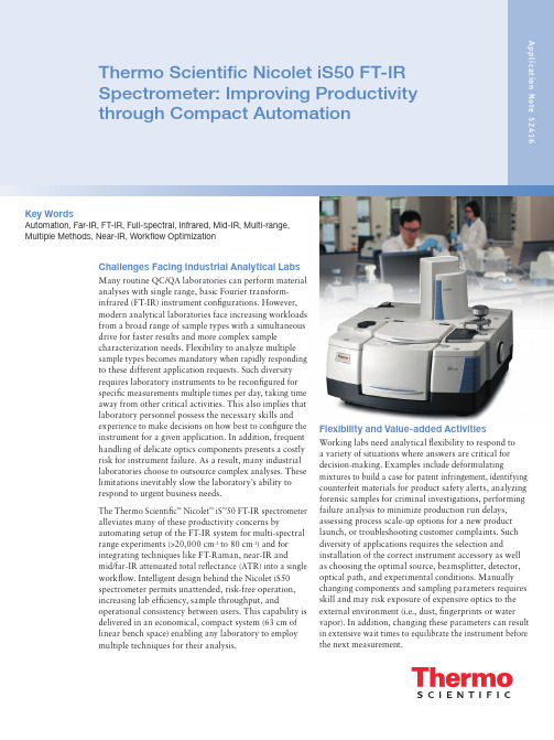
Thermo Scientific Nicolet iS50 FT-IRSpectrometer: Improving Productivity through Compact Automation Application Note 52416 Key WordsAutomation, Far-IR, FT-IR, Full-spectral, Infrared, Mid-IR, Multi-range,Multiple Methods, Near-IR, Workflow OptimizationChallenges Facing Industrial Analytical LabsMany routine QC/QA laboratories can perform materialanalyses with single range, basic Fourier transform-infrared (FT-IR) instrument configurations. However,modern analytical laboratories face increasing workloadsfrom a broad range of sample types with a simultaneousdrive for faster results and more complex samplecharacterization needs. Flexibility to analyze multiplesample types becomes mandatory when rapidly respondingto these different application requests. Such diversityrequires laboratory instruments to be reconfigured forspecific measurements multiple times per day, taking timeaway from other critical activities. This also implies thatlaboratory personnel possess the necessary skills andexperience to make decisions on how best to configure the instrument for a given application. In addition, frequent handling of delicate optics components presents a costly risk for instrument failure. As a result, many industrial laboratories choose to outsource complex analyses. These limitations inevitably slow the laboratory’s ability to respond to urgent business needs.The Thermo Scientific™ Nicolet™ iS™50 FT-IR spectrometer alleviates many of these productivity concerns by automating setup of the FT-IR system for multi-spectral range experiments (>20,000 cm-1 to 80 cm-1) and fori ntegrating techniques like FT-Raman, near-IR and mid/far-IR attenuated total reflectance (ATR) into a single workflow. Intelligent design behind the Nicolet iS50 spectrometer permits unattended, risk-free operation, increasing lab efficiency, sample throughput, and operational consistency between users. This capability is delivered in an economical, compact system (63 cm of linear bench space) enabling any laboratory to employ multiple techniques for their analysis.Flexibility and Value-added ActivitiesWorking labs need analytical flexibility to respond toa variety of situations where answers are critical for decision-making. Examples include deformulating mixtures to build a case for patent infringement, identifying counterfeit materials for product safety alerts, analyzing forensic samples for criminal investigations, performing failure analysis to minimize production run delays, assessing process scale-up options for a new product launch, or troubleshooting customer complaints. Such diversity of applications requires the selection and installation of the correct instrument accessory as well as choosing the optimal source, beamsplitter, detector, optical path, and experimental conditions. Manually changing components and sampling parameters requires skill and may risk exposure of expensive optics to the external environment (i.e., dust, fingerprints or water vapor). In addition, changing these parameters can result in extensive wait times to equilibrate the instrument before the next measurement.These manual reconfigurations provide little added value to the laboratory workflow. Users must plan and set up batch experiments to minimize the number of steps. This creates bottlenecks, limiting access to the full capability of the instrument. As a result, labs are less able to address “emergency situations” without interrupting the batch run and resetting the instrument parameters. For instance, analysis of a polymer with additives requires mid-IR and far-IR plus Raman spectroscopy. This would entail three beamsplitter changes with associated risks in handling expensive components and instrument recovery times between changes.The productivity improvements with the Nicolet iS50 FT-IR spectrometer come from two main sources. First, the internally mounted iS50 ABX Automated Beamsplitter Exchanger uses one-button simplicity (described as a Touch Point) to perform instrument setup and operation, providing a “one touch and done” workflow. The removal of manual handling and exposure of the optics to the environment means instant readiness. Second, the user need no longer care about which optics are installed. As seen in Table 1, the potential for error in manual operations is apparent when the array of possible component combinations is considered. With the Nicolet iS50 spectrometer, however, a user simply presses the Touch Point on the instrument to automate the configuration and ready the instrument for the experiment. For example, pressing the Touch Point on the iS50 NIR module automates the setup without requiring any understanding of which optics are used. What matters is performing NIR analysis – not worrying about choosing the right components. The instrument takes care of this step. Integration of the spectrometer with its modules and components allows the user to expand capabilities, increasing productivity with tools such as:• Up to three detectors (such as near-, mid- and far-IR)• The iS50 Raman sample compartment module• The built-in diamond iS50 ATR sampling station• T he iS50 NIR module with integrating sphere or fiber optics• The iS50 GC-IR module• A sample compartment thermal gravimetric analysis-IR (TGA-IR Interface)Figure 1 describes the analytical power the user can achieve with the iS50 spectrometer to obtain answers needed for time-sensitive decisions. With a single user interaction, the instrument can perform multiple measurements and analyses, resulting in a final report, even when unattended. The Thermo Scientific OMNIC™software provides a user-friendly interface to set up applications quickly and generate spectra for definitive answers. By adding powerful analytical tools like the Thermo Scientific OMNIC Specta™ software with a library of over 30,000 spectra and multi-component searching (or the TQ Analyst™ software for chemometrics), a complete analytical workflow from sampling to results can often be achieved in less than 60 seconds.This paper will demonstrate how the integration and automation of the Nicolet iS50 spectrometer leads to new levels of productivity, while minimizing risk to costly components. Unlike most spectrometers, operating the Nicolet iS50 instrument becomes simpler as modules are added and as more manual steps are removed even when unattended.Experiment Source Beamsplitter Detector AccessoryMid-IR Transmission Thermo Scientific Polaris™KBr KBr-DLaTGS Standard Cells Far-IR Transmission Polaris Solid Substrate Polyethylene DLaTGS Cells w/Far-IR Windows Near-IR Transmission White Light CaF2InGaAs CuvettesMid-IR ATR Polaris KBr Dedicated DLaTGS iS50 ATRFar-IR ATR Polaris Solid Substrate Dedicated DLaTGS iS50 ATRFT-Raman Raman Laser CaF2Raman InGaAs iS50 RamanTable 1: Experiments made possible with the Nicolet iS50 FT-IR SpectrometerFigure 1: Nicolet iS50 analysis workflowAutomated Multi-spectral Analysis:Mid- and Far-IR ATR plus Near-IRMost FT-IR users understand the utility of the mid-IR spectral range for qualitative and quantitative analyses. Less well known, the far-IR region can provide new and unique information. Simply put, as the mass of atoms involved in vibrations increases, the wavenumber decreases.1Thus, for materials like organometallics or metal oxides, the IR absorption shifts below 400 cm-1 and below the range of standard KBr optics. Numerous polymers, sugars, and other large molecules also have far-IR information which may be useful or definitive to the analyst. Traditionally, collecting FT-IR spectra in both the mid-IR and far-IR region entailed significant sample preparation. This included changing hygroscopic optics and multiple detectors, and risking altered system performance from water vapor. The Nicolet iS50 spectrometer enables rapid analysis over the full mid-IR and well into thefar-IR region (4,000 cm-1 to 80 cm-1) when equipped with the iS50 ABX, iS50 ATR, and the correct beamsplitters. The typical, multi-range FT-IR application requires opening the spectrometer to swap beamsplitters. This requires care in handling costly components and exposesthe internal optics to the environment by disrupting purge or desiccation. This activity adds a recovery period tore-equilibrate the instrument before quality data can be collected. These wait times add no value to operations, wasting the analyst’s precious time. Integration and automation on the spectrometer eliminate non-productive wait times, improving efficiency.As an example, Table 2 compares the steps needed to perform a full spectral analysis from far-IR to near-IR between the manual method (Typical) and the Nicolet iS50 method with built-in iS50 ATR and iS50 NIR module. This represents three spectral ranges in one sampling operation, a unique power of the instrument. Most important the built-in iS50 ATR optics and detector permit spectral data collection in both the mid- and far-IR regions. The analysis time decreases from around 30 minutes to less than seven. With the Nicolet iS50 spectrometer, the user is able to load two sampling locations (the built-in ATR and the Integrating Sphere module), start the macro and walk away, while in the manual operation, continuous attention is needed to swap the beamsplitters at the right moments. This seemingly hidden improvement allows unattended operation, permitting productivity through automation. Figure 2 shows just the mid- and far-IR spectra collected from acetylferrocene analyzed using an OMNIC macro-controlled workflow. The additional information from the far-IR spectra is clear – the low end triplet verifies that the iron is sandwiched between the cyclopentadiene rings. The NIR data is not shown, but the entire process required seven minutes, including collection of themid- and far-IR backgrounds. Automation also reduced the total hands-on time of the user (pressing buttons, loading sample) to ≈20 seconds. Figure 2: Mid-IR and far-IR spectra of Acetylferrocene. The far-IR optics permit collection to 1700 cm-1, which may be sufficient (fingerprint and far-IR) for many applications.Time Nicolet iS50 Time Process Step Typical (minutes) with Built-in ATR (minutes) Sample Preparation Grind, Mix 10 None 0 Mid-IR Background Collect BKG 0.5 Collect BKG (2nd)* 1. Mid-IR Collect Load Sample, 2 Load Sample, 1Collect Spectrum Collect SpectrumChange Optics Manual Exchange 0.5 Automated 0.5 Recovery Time Wait for Purge 5–10 No Recovery Time 0 Far-IR Background Collect BKG 0.5 Collect BKG (1st)* 0.5 Far-IR Collect Load Sample, 2 Load Sample, 1Collect Spectrum Collect SpectrumChange Optics (NIR) Manual Exchange 0.5 Automated 0.5 Recovery Time Wait for Purge 5 No Recovery Time 0 Collect Background Collect BKG 0.5 Collect BKG 0.5 Collect Sample Load Sample, 1 Collect SAM 0.5Collect SAMData Analysis (Search) Perform Search 2 Automated Search 0.5 Total Time 29.5–34.5 6.5 Table 2: Far-infrared analysis: Typical versus Nicolet iS50 process* W ith the iS50 ATR present, the far-IR background (BKG) is collected, the iS50 ABX swaps beamsplitters, and themid-IR background is collected in <1.5 minutes. The sample is loaded and the spectra are collected in sequence.All times are approximate.Figure 3: The Thermo Scientific Nicolet iS50 FT-IR spectrometer configured for FT-Raman, near-IR, and mid/far-IR ATR with the automated beamsplitter exchanger.Figure 4: Touch Points on the Nicolet iS50 spectrometer employ one-button switching between modules and the iS50 ABX automates optics set-up Touch Point A – NIR module Touch Point B – Raman moduleTouch Point C – Built-in diamond ATRComponent D – ABX Automated Beamsplitter ExchangerMultiple Techniques and Multi-range Analysis: Enhanced FlexibilityThe Nicolet iS50 spectrometer can be configured with FT-Raman, NIR, and wide-range diamond ATR. Switching between these experiments raises concerns of instrument recovery time (purge), exposure/handling of optics, and potential confusion or user error. The experiments are often seen as independent activities for these reasons. The spectrometer with iS50 ABX simplifies this apparently complex situation to one step – initiation of a macro. The Nicolet iS50 instrument shown in Figure 3 is configured with the iS50 NIR, iS50 Raman, iS50 ATR and the iS50 ABX modules and shows how easy sample loading and analysis can be done.For operating one module at a time, the user need only press the associated Touch Point. Seen more closely in Figure 4, Touch Points make one-button operation effortless when switching between modules (sampling stations) and automating optics exchange. Rather than thinking through the components needed (light source, beamsplitter, optical path and detector) to run anexperiment, the user simply presses the Touch Point to switch from an ATR to an NIR measurement and waits until the instrument indicates that it is ready to begin. This error-free operation is done in 30 seconds.The Nicolet iS50 analytical power in Figure 1 becomes clear when the four data collections – mid-IR and far-IR ATR, NIR, and Raman – are performed in one workflow. Collecting spectra from each of these modules using a conventional manual approach required about 50 minutes, including sample loading, optical changes, time forequilibration, and optimization of the Raman signal. The analyst needed to be present throughout the experiment to perform the beamsplitter changes and collect various backgrounds for each sampling station. At the end of the 50 minutes, four spectra and their analyses were available. Actual data collection took 5 minutes and total hands-on time was 45 minutes, representing inefficient use of the analyst’s time.In contrast, the results shown in Figure 5 emerged from a single OMNIC-macro operation. The macro wasprogrammed to begin by collecting backgrounds for the mid- and far-IR ATR, and then switched to the iS50 Raman module. Next the samples were loaded on the ATR, NIR, and Raman sampling stations. After optimizing the signal using the autofocus feature of the Ramanmodule, the macro was initiated, and the analyst walked away. From starting the macro to completion of the final report, the analysis took less than 12 minutes, representing a time savings of over 70%. The actual data collection time was again 5 minutes, however, total hands-on time for the analyst was only 2 minutes – a highly efficient use of the analyst’s (and the instrument’s) time.ABC DApplication Note 52416AN52416_E 12/12MAfrica +27 11 822 4120Australia +61 3 9757 4300Austria +43 1 333 50 34 0Belgium +32 53 73 42 41Canada +1 800 530 8447China +86 10 8419 3588Denmark +45 70 23 62 60Europe-Other +43 1 333 50 34 0Finland/Norway/Sweden +46 8 556 468 00France +33 1 60 92 48 00Germany +49 6103 408 1014India +91 22 6742 9434Italy +39 02 950 591Japan +81 45 453 9100Latin America +1 561 688 8700Middle East +43 1 333 50 34 0Netherlands +31 76 579 55 55New Zealand +64 9 980 6700Russia/CIS +43 1 333 50 34 0Spain +34 914 845 965Switzerland +41 61 716 77 00UK +44 1442 233555USA +1 800 532 4752©2012 Thermo Fisher Scientific Inc. All rights reserved. All trademarks are the property of Thermo Fisher Scientific Inc. and its subsidiaries.This information is presented as an example of the capabilities of Thermo Fisher Scientific Inc. products. It is not intended to encourage use of these products in any manners that might infringe the intellectual property rights of others. Specifications, terms and pricing are subject to change. Not all products are available in all countries. Please consult your local sales representative for details.ConclusionMany forces contribute to new pressures on industrial analytical laboratories: increased sample loads, decreased staffing, retirement of experts, and shrinking budgets. The Thermo Scientific Nicolet iS50 FT-IR spectrometer makes a significant contribution to alleviating these challenges through automation in a multi-tasking, single platform instrument. The Nicolet iS50 spectrometer greatly simplifies and streamlines workflows by decreasing the number of steps with one-button ease and macro operations performed by the analyst. In addition, risks inherent in manual operations (e.g., user error, environmentalexposure) and long recovery times are eliminated. Analysts of any skill level can successfully obtain meaningful results with minimal hands-on time.Technology designed to improve workflow can be found in the iS50 ABX and task-specific modules (i.e., Raman, NIR, TGA-IR etc.). The Touch Point operation simplifies access to the full range of capabilities by automatically configuring the optics (near-, mid- and far-IR) andswitching between sampling stations (modules) in secondsfor enhanced productivity. For the modern industrial lab, the Nicolet iS50 FT-IR spectrometer offers a powerful new tool that goes beyond routine FT-IR to more comprehensive analyses (e.g., FT-Raman and far-IR), adding value to laboratory activities in a compact, easy-to-operate platform.References1. H eavy atoms or groups of atoms shift the IR wavenumber value lower, according to the relationshipwhere ˜v is the IR wavenumber (cm -1) and μ is the reduced mass. As the mass (μ) increases, the IR peak shifts to lower wavenumbers.GlossaryCaF 2– calcium fluorideDLaTGS – d euterated L-alanine doped triglycene sulphate InGaAs – Indium gallium arsenide KBr– potassium bromideFigure 5: Multi-technique data for a recyclable plastic component using the spectrometer pictured in Figure 3. Inset shows NIRindependently for clarity.。
基于高精度光学腔测量气体中痕微量NO_(2)的方法

第46卷第2期 2021年4月天然气化工一C1化学与化工NATURAL GAS CHEMICAL INDUSTRYVol.46 No.2Apr. 2021•开发应用•基于高精度光学腔测量气体中痕/微量NO2的方法唐霞梅,谭依玲,成雪清,李威,徐龙,王少楠(西南化工研究设计院有限公司,四川成都610225)摘要:以吸收光谱为基础的高精度光学腔气体检测技术用于大气中痕量NO。
气体的分析具有在线、实时、高灵敏度等优 点。
分析了近年来NOx排放情况和主要排放源,并针对采用其他光学仪器测量NO2时存在稳定性不好、受标样影响等问题,搭建 了一套适合在线分析N〇2的测量装置;通过仿真选择了 1630.33 cm-1光谱吸收段用于N〇2的测量,利用Allan方差分析评估了系统 的稳定性。
结果表明,在积分时间为200 s时,对应的最低检测限为3.1 x 10鄄9(体积分数)。
将该装置应用于西部某煤化工企业的 燃煤烟道气中N〇2浓度的检测和分析,其结果与实际情况高度吻合。
关键词:痕/微量N〇2;气体检测;高精密光学腔中图分类号:TQ116.02 文献标志码:A 文章编号:1001-9219(2021)02-104-05Method of measuring trace N〇2 in flue gas based on high-precision optical cavity TANG Xia-mei, TAN Yi-ling, CHENG Xue-qing, LI Wei, XU Long, WANG Shao-nan(Southwest Institute of Chemical Co., Ltd., Chengdu 610225, Sichuan, China)Abstract: High precision optical cavity gas detection technology based on absorption spectrum has the advantages of on-line, real-time and high sensitivity for the analysis of trace N〇2 gas in the atmosphere. The emission status and main emission sources of N〇x in recent years were analyzed, and a set of measurement equipment suitable for online analysis was built to solve the problems of poor stability and standard sample influence in the measurement of N〇2 with other optical instruments. The 1630.33 cm-1spectral absorption band was selected for N〇2 measurement by simulation, and the system stability is evaluated by Allan variance analysis. The results showed that the minimum detection limit is 3.1 x 10⁹(volume fraction) when the integration time was 200 seconds. The device was applied to the detection and analysis of N〇2 concentration in the flue gas of a modern coal chemical production enterprise in Western region, and the results were highly consistent with the actual situation.Keywords: trace N〇2; gas detection; high-precision optical cavity随着我国工业化进程的加速,环境污染问题日 益严峻,发展大气污染物的检测技术,对环境污染 的监控、治理以及环境科学问题的研究具有重要意 义[1]。
二氧化硅介孔

Journal of Molecular Catalysis A:Chemical264(2007)153–161Preparation of mesoporous silica/polymer sulfonate composite materials Masahiro Fujiwara a,∗,Kumi Shiokawa a,Yingchun Zhu ba Kansai Center,National Institute of Advanced Industrial Science and Technology(AIST),1-8-31Midorigaoka,Ikeda,Osaka563-8577,Japanb Shanghai Institute of Ceramics,Chinese Academy of Sciences,Shanghai200050,People’s Republic of ChinaReceived21June2006;received in revised form22August2006;accepted9September2006Available online15September2006AbstractMesoporous silica/polymer sulfonate composite materials were prepared by simply mixing hexadecyltrimethylammonium bromide,polymer sulfonates and TEOS(tetraethoxysilane)in alkaline aqueous solution.Nafion and poly(sodium4-styrenesulfonate)were employed as polymer sulfonates.XRD patterns and nitrogen adsorption–desorption isotherms showed that the precipitates obtained had mesostructure similar to MCM-41.Especially,the crystallinity of hexagonal structure of composite materials synthesized with Nafion was high.From all the results obtained here, it is concluded that the polymer sulfonate resins might be incorporated in the wall framework of mesoporous silica matrix.However,when the excess amount of Nafion was mixed,the acid sites of Nafion were significantly lost in the obtained materials.These composite materials present new classes of organically modified mesoporous silicas,where organic polymers are incorporated in the framework of mesoporous silica.They were used as catalysts for␣-methylstyrene dimerization and Friedel–Crafts alkylation reaction of aromatics.©2006Elsevier B.V.All rights reserved.Keywords:Mesoporous silica;Nafion;Poly(styrenesulfonate);Nano-composite;Solid acid;␣-Methylstyrene dimerization1.IntroductionResearches on mesoporous silicas and related materials are importantfields of recent material science[1,2].Especially MCM-41and its analogues[2]are actively studied because of their high potentials for various applications.The function-alization of mesoporous silica with organic compounds began with the surface modification using silane compounds such as R-Si(OR )3[1,3].After this kind of approach,the framework modification using disilane compounds followed.These materi-als are often called periodic mesoporous organosilicas(PMOs) [4–6].For example,Inagaki and co-workers notified that ben-zene ring and analogues are completely incorporated into the framework of mesoporous silica materials,and that these mate-rials are effective acid catalysts after sulphonation[7].Another trend is the polymerizations in the pore voids of mesoporous materials:many researchers produced composite materials with the corresponding polymers by this method[8].Mesoporous composite materials,where an organic polymer is introduced into their“framework”,are also investigated.In2000,we briefly ∗Corresponding author.Tel.:+81727519253.E-mail address:m-fujiwara@aist.go.jp(M.Fujiwara).reported that Nafion resin,whose structure is illustrated inFig.1,was incorporated in the framework of M41S type ofmesoporous silica[9].This material was a unique catalyst for ␣-methylstyrene dimerization.Recently,another group devel-oped the composite materials with polyacrylate[10].In Fig.2,a classification of these composite materials of mesoporous sil-ica with organic components is proposed.Type(A)is surfacemodification using R-Si(OR )3compounds[1,3],and Type(B)isframework modification such as periodic mesoporous organosil-icas(PMOs)[4–7].Type(C)shows composite materials withpolymeric compounds in the pore voids[8].Composite meso-porous materials with polymers in the framework are namedType(D)here[9,10].In this paper,we wish to report further examination of thecomposite materials of mesoporous silica with Nafion resin.Thematrices of mesoporous materials are expected to offer orderednanostructures useful as solid support[11].Nafion resin is alsoa functional perfluorinated sulfonic acid polymer to be usedas acid catalyst[12]and as polymer electrolyte for fuel cellapplication[13].Composite materials of Nafion resin with amor-phous silica have been utilized in these technologies[14,15].The ordered nanostructures of Nafion and analogous resins withmesoporous silica matrix are expected to be useful for variousapplications.1381-1169/$–see front matter©2006Elsevier B.V.All rights reserved. doi:10.1016/j.molcata.2006.09.016154M.Fujiwara et al./Journal of Molecular Catalysis A:Chemical264(2007)153–161Fig.1.Structure of Nafion resin.2.Experimental2.1.Preparation of mesoporous silica/Nafion composite materialThe preparation procedure is considerably simplified from our previously reported method[9].Nafion solution commer-cial available was directly used and no hydrothermal treatment was performed.A typical synthesis of mesoporous silica/Nafion composite is following:5.0g of5%Nafion alcohol solution (from Aldrich)was added to200mL of the aqueous solution of NaOH(1.73g;43.25mmol)and hexadecyltrimethylammo-nium bromide(3.48g;9.55mmol),and this mixed solution was stirred for a few minutes.To this solution,16.69g(80mmol) of tetraethoxysilane(TEOS)was added dropwise for5min, and the resulting solution was further stirred for12h at room temperature.An as-synthesized sample thus obtained wasfil-tered,washed with sufficient amount of H2O and dried at80◦C for12h.Template was removed by refluxing with1M H2SO4 solution of EtOH(solid sample/EtOH solution=1g/150mL)for 12h.Thefiltered solid was refluxed again with pure EtOH(sam-ple/EtOH=1g/150mL)for12h,filtered,washed with H2O at room temperature and dried at80◦C for12h.2.2.Preparation of mesoporous silica/Nafion composite material from amorphous silica/Nafion compositeThe general preparation method of MCM-41type of meso-porous silica from porous amorphous silica is described in elsewhere[16].This procedure was applied to amorphous sil-ica/Nafion composite.The amorphous silica/Nafion composite used here was SAC-13purchased from Aldrich.To the aqueous solution of NaOH(0.15g;3.80mmol)with hexadecyltrimethy-lammonium bromide(0.37g;1.00mmol)in4mL of H2O,0.61g of SAC-13was added.After stirred for1h,the resulting mixture was placed in a stainless autoclave,sealed tightly and heated at 110◦C for24h under autogenous pressure.The following pro-cedures were similar to the above-mentioned process.2.3.Preparation of mesoporoussilica/poly(4-styrenesulfonate)composite materialTo the solution of NaOH(0.799g;19.98mmol)and hex-adecyltrimethylammonium bromide(1.582g;4.341mmol)in 90mL of H2O,0.412g of poly(sodium4-styrenesulfonate)dis-solved in10mL of H2O was added,and to this homogeneous solution8.403g(40.34mmol)of TEOS was mixed.The result-ing solution was stirred for2days at ambient temperature. The precipitate thus formed wasfiltered,washed with sufficient amount of H2O and air-dried.The following procedures were similar to the above-mentioned process.2.4.Preparation of mixture of Nafion with hexadecyltrimethylammonium bromideA5%alcohol solution of Nafion(7.656g;Nafion content: 0.353g;sulfonic acid equivalent:0.341mmol)was mixed with NaOH(0.038g:0.95mmol)in5mL of H2O.After removing solvent under reduced pressure,the residue was dissolved in a mixed solution of H2O(10mL)and EtOH(10mL).Finally hexadecyltrimethylammonium bromide(0.125g;0.343mmol) was added.After about1day,white precipitate obtained was filtered and air-dried.2.5.Preparation of mixture of poly(4-styrenesulfonate)with hexadecyltrimethylammonium bromideThe solution of0.412g of poly(sodium4-styrenesulfonate) in6mL of H2O was mixed with the aqueous solution(50mL)of hexadecyltrimethylammonium bromide(0.728g;2.00mmol). The white precipitate was formed in a few minutes.After stirring for1h,the white precipitate wasfiltered and dried at60◦C. 2.6.Product characterizationsXRD patterns were recorded with a MAC Science MXP3V diffraction apparatus with Nifiltered Cu K␣radiation (λ=0.15406nm).N2adsorption-desorption isotherms were obtained at−196◦C(in liquid N2)using a Bellsorp Mini instru-ment(BEL JAPAN Inc.).BJH calculation was performed toesti-Fig.2.Conceptual schemes of composite materials of mesoporous silica with organic components.M.Fujiwara et al./Journal of Molecular Catalysis A:Chemical264(2007)153–161155mate the mesopore size using adsorption branches of isotherms. Elemental analyses of silicon were performed by the alkali fusion-gravimetric method according to JIS G1212(Japanese industrial standard).Elemental analyses offluorine were car-ried out with the lanthanum-alizarin complexone method using a Shimadzu UV-1600photometry apparatus after the extraction of alkali fusion method.Elemental analyses of carbon were per-formed by the common combustion gas quantification method. Thermogravimetric analyses(TGA)were performed on a Shi-madzu TGA-50apparatus.All samples were held in a platinum sample holder and were heated under air from room temperature to800◦C at the rate of5◦C/min.FT-IR spectra were mea-sured on a Perkin-Elmer Spectrum One spectrometer.Transmit-tance electron microscope(TEM)images were obtained using a JEM-2100F(JEOL)high-resolution transmissionfield emis-sion electron microscope(HRTEM)operated at300kV.The acid capacities of composite materials were estimated by the titra-tion method.The composite materials were immersed in0.1M of aqueous solution of NaCl,and the acid amounts of the ion-exchanged solutions thus obtained were analyzed by titrating with0.01M NaOH using phenolphthalein as indicator.2.7.Catalytic reactionsThe experimental procedure of␣-methylstyrene(AMS) dimerization was described in our previous paper[9].A com-petitive Friedel–Crafts reaction of toluene and p-xylene with benzyl alcohol was performed by the mixed solution of toluene (0.92g,10mmol),p-xylene(1.05g,10mmol)and benzyl alco-hol(0.22g,2mmol)in the presence of a catalyst(0.05g)at 90◦C for7h with vigorous stirring.Afterfiltering the catalyst, thefiltrate was analyzed by a capillary GC.3.Results and discussion3.1.Synthesis of mesoporous silica/Nafion composite materialComposite materials made of mesoporous silica and Nafion resin were prepared by a procedure modified formesoporous Fig.3.XRD patterns of as-synthesized and template-free(solvent extracted) mesoporous silica/Nafion composite materials.(A)As-synthesized MCM/ Nafion-1.(B)As-synthesized MCM/Nafion-2.(C)Template-free MCM/Nafion-1.(D)Template-free MCM/Nafion-2.silica synthesis.TEOS was added to a homogeneous alkaline solution of hexadecyltrimethylammonium bromide with Nafion resin.After stirring at room temperature,as-synthesized com-posite materials of mesoporous silica and Nafion resin were obtained as a white precipitate.Although hydrothermal treat-ment in an autoclave was given in our previous paper[9],we found that this hydrothermal treatment is not essential for the synthesis after the publication of the paper.The surfactant as template was removed by refluxing in H2SO4–EtOH solution (1M of H2SO4).H2SO4is expected to contribute to both the regeneration of sulfonic acid sites in Nafion polymer resin and the surfactant removal.The sample names and the profiles of composite materials are summarized in Table1.The data of a composite material prepared under hydrothermal conditions[9] are also included in Table1as MCM/Nafion-H.Fig.3shows XRD patterns of two composite materials(MCM/Nafion-1andTable1Properties of various mesoporous silica/polymer composites materialsSample Starting ratio d100a SSA b(m2/g)PV c(cm3/g)PPD d(nm) g/mol e wt%f2θnmMCM/Nafion-1 3.13 5.21 2.32(2.34) 3.81(3.77)1239 1.12 2.52 MCM/Nafion-2 6.7211.18 2.20(2.22) 4.01(3.98)1211 1.26 2.75 MCM/Nafion-314.8724.76 2.20(2.28) 4.01(3.87)3330.26 2.52 MCM/Nafion-H g 6.5810.96 2.25(2.35) 3.92(3.76)918 1.00 2.75 MCM/PSS8.8815.19 2.14(2.24) 4.13(3.94)8380.66 2.75a d100:X-ray diffraction(100)interplanar spacing.In parentheses,as-synthesized sample.b BET specific surface area.c Primary mesopore volume calculated from adsorption branch of BJH pore size distribution curve.d Peak pore diameter from adsorption branch of BJH pore size distribution curve.e Starting ratio of polymer(as acid type)and TEOS;gram of polymer/molar of TEOS.f Estimated weight percentage when polymer is completely incorporated in solid material and all TEOS converts into silica(SiO2).g MCM/Nafion composite material we reported[9].156M.Fujiwara et al./Journal of Molecular Catalysis A:Chemical264(2007)153–161Fig.4.Infrared spectra of as-synthesized(A)and template-free(B)MCM/ Nafion-1composite material.MCM/Nafion-2)in as-synthesized and template-free forms. XRD patterns indicated the formation of the hexagonal structure characteristically observed in the MCM-41type of mesoporous silica[2].The peaks assigned to d110,d200and d210interpla-nar spacings were found besides those from d100interplanar ones in all four samples.The surfactants were removed success-fully by the extraction using H2SO4in EtOH with the hexagonal structure maintained.Template removal by calcination was not performed to avoid thermal decomposition of Nafion resin.The peaks derived from the hexagonally ordered structure became stronger after the template removal in both cases(MCM/Nafion-1and MCM/Nafion-2).Infrared spectra of as-synthesized and template-free (extracted)samples are shown in Fig.4.In the as-synthesized sample,strong absorptions of the surfactant were observed approximately at2929and2850cm−1(Fig.4A).These absorp-tions disappeared after the treatment with H2SO4(Fig.4B), indicating the complete removal of the surfactant.On the other hand,the absorptions of C–F stretching modes of Nafion resin at1210and1160cm−1were not found in either spectra,while they are detected in amorphous silica/Nafion composite[14a]. It seems that in the case of amorphous silica/Nafion compos-ite,the contact time of Nafion resin with alkaline solution is comparatively short(the preparation solution gels immediately), preventing the serious decomposition of C–F bonds[14a].In our case,Nafion resin was dissolved in the high alkaline solution for a long time,resulting in critical degradation.The TEM images of MCM/Nafion-1are shown in Fig.5.The ordered structure(hexagonally arranged)was confirmed from the layered lines in the solid.The distance between layers is estimated to be3.0–3.8nm,approximately according with that from XRD patterns.The nitrogen adsorption–desorption isotherms of the template-free samples are shown in Fig.6.Both samples, MCM/Nafion-1and MCM/Nafion-2,indicated the typical type IV isotherms(IUPAC)of ordered mesoporous silica materi-als.The pore size of MCM/Nafion-2was larger than that of MCM/Nafion-1.These results were consistent with the d100 interplanar spacings from XRD patterns(Fig.3).Specific sur-face areas(BET surface area)and pore volumes of both samples were over1000m2/g and1cm3/g,respectively.These data were at the level similar to the MCM-41type of mesoporous sil-icas[1,2],and considerably higher than those of amorphous silica/Nafion composite materials[15].These properties are similar to those of the sample prepared under hydrothermal con-ditions(MCM/Nafion-H)in our previous paper[9].Therefore, a simpler preparation method using the direct use of commer-cial reagent under ambient conditions proved to be applicable. However,when more than20wt%of Nafion resin was added to the starting solution,the ordered structure of the corresponding composite material was considerably collapsed(MCM/Nafion-3).The peak at2.28in2θobserved in the as-synthesized sample (Fig.7A)indicated its moderately ordered structure.However, this peak almost disappeared after the removal of template (Fig.7A),showing the destruction of the ordered structure. In Fig.7B,the nitrogen adsorption–desorption isotherm and the pore size distribution estimated from the BJH method of template-free MCM/Nafion-3are presented.The porosity of this sample was poor and the peak of the pore diameterwas Fig.5.TEM images of MCM/Nafion-1(template-free).M.Fujiwara et al./Journal of Molecular Catalysis A:Chemical264(2007)153–161157Fig.6.(A)Nitrogen adsorption–desorption isotherms of mesoporous silica/Nafion composite materials.( )Adsorption branch of MCM/Nafion-1;( )desorption branch of MCM/Nafion-1;( )adsorption branch of MCM/Nafion-2;(᭹)desorption branch of MCM/Nafion-2.(B)Pore size distributions estimated from the adsorption branches of the isotherms by BJH method.( )MCM/Nafion-1;( )MCM/Nafion-2.broad.The specific surface area and the pore volume decreased to333m2/g and0.259cm3/g,respectively.Thus,the addition of excess amount of Nafion resin inhibited the formation of ordered structure.Another approach to the preparation of the composite mate-rial was attempted by using an amorphous silica/Nafion com-posite.It is well known that porous amorphous silica can be transformed into mesoporous MCM-41type material in the pres-ence of surfactant in alkaline solution[2,16].An amorphous silica/Nafion composite material commercially available(SAC-13;Nafion content:approximately13wt%)was immersed in an alkaline solution dissolving hexadecyltrimethylammonium bromide.This solution system was placed in an autoclave to be hydrothermally treated by reacted at115◦C for24h[16]. The XRD patterns of as-synthesized and template-free samples thus obtained are shown in Fig.8.The crystallinity of the as-synthesized sample was poor,and after the removal of template the hexagonal structure nearly collapsed.Even in this case,a comparatively high content of Nafion resin(13wt%)is thought to prevent the formation of ordered structure in the case of MCM/Nafion-3.3.2.Analyses of composition of mesoporous silica/Nafion composite materialThe contents of Nafion resin in these composite materials were analyzed by various methods.The results of TGA measure-ment of these composite materials are listed in Table2.Nafion resin is thermally decomposed from150to600◦C[17],and the weight decrease of pure mesoporous silica(without Nafion resin)we prepared was measured4.78%due to the thermal dehydration of silanols in this temperature range.The corrected values of the weight decreases by this blank measurement are shown in the parentheses.Although there are no direct propor-tional relationships between the starting contents of Nafion and the weight decreases,combustible Nafion contents increased from MCM/Nafion-1to MCM/Nafion-3.A similar tendency was observed in the elemental analysis shown in Table2.The Fig.7.(A)XRD patterns of as-synthesized and template-free(solvent extracted)MCM/Nafion-3.(B)Nitrogen adsorption–desorption isotherm and the pore size distribution by BJH method from adsorption branch(in inset)of MCM/Nafion-3.158M.Fujiwara et al./Journal of Molecular Catalysis A:Chemical264(2007)153–161Fig.8.XRD patterns of as-synthesized(A)and template-free(B)mesoporous silica/Nafion composite material obtained from an amorphous silica/Nafion composite(SAC-13).carbon andfluorine contents increased with the starting Nafion resin contents.It should be noted that thefluorine contents were low in these composite materials,although the weight ratios of fluorine to carbon must be approximately3.2according to the chemical formula of Nafion(Fig.2)[14a].These lower con-tents offluorine indicated that carbon–fluorine bonds in Nafion resin were significantly cleaved during the preparation process, because aliphatic perfluoro group is known to be unstable under basic conditions(although aromatic C–F bond is reported to be tolerant in alkaline solution)[11a].No observation of C–F bonds in infrared spectra(Fig.4),which can be observed in amorphous silica/Nafion composite[14a],was likely to result from the decrease in thefluorine content in the resin.The acid capacities of these composite materials were estimated by the cation exchange method with NaCl[14].The acid equivalents are also summarized in Table2.The acid content of pure Si-MCM-41(with Nafion resin)was under 0.001mequiv.H+/g.Pure Nafion resin(NR-50)and its compos-ite material with amorphous silica(SAC-13;Nafion content: 13wt%)is reported to have0.89or0.14mequiv.H+/g of acid capacities,respectively[14].In the parentheses of Table2, the weight percentages of Nafion in the composite materials calculated from the measured acid capacities are listed on the assumption that all sulfonic acid sites of Nafion resin are active. The calculated Nafion content of MCM/Nafion-1(5.92wt%) from acid capacity was reasonably consistent with the estimated values from both starting ratio and TGA measurement.On the other hand,in the case of MCM/Nafion-2,the Nafion content estimated from the acid capacity(17.02wt%)was in discord with other results.Furthermore,the acid capacity of MCM/Nafion-3was approximately0.003mequiv.H+/g.From these results,it was concluded that high contents of Nafion in the composite materials led to the some decomposition of Nafion resin,while no significant changes were observed in the case of low Nafion contents.3.3.Synthesis of mesoporous silica/poly-sulfonate composite materialThe formation of composite materials of mesoporous silica with polyacrylate was recently claimed in a report[10],where a procedure analogous to ours was used.We also studied the prepa-ration of a composite material made of mesoporous silica and another poly-sulfonate.Poly(4-styrenesulfonic acid)sodium salt was employed for the synthesis.In a similar manner to Nafion, TEOS was added to the mixed alkaline solution of poly(sodium 4-styrenesulfonate)(PSS)and hexadecyltrimethylammonium bromide,forming a composite material(MCM/PSS)after stir-ring.The XRD patterns of the as-synthesized and template-free samples are shown in Fig.9A.Although the peak intensities of these two patterns were lower than those of composite materials with Nafion,an ordered structure in the nano-level was observed. In the as-synthesized MCM/PSS,peaks assigned to d110,d200 and d210interplanar spacings were found as well as d100inter-planar one.Those peaks are not so clear in the template-free MCM/PSS,and its pore structure might be a wormhole like one[18].The nitrogen adsorption–desorption isotherms of this MCM/PSS composite material presented in Fig.9B are basi-cally type IV.The peak pore diameter was found at2.75nm (in inset).Thus,a poly(styrenesulfonate)polymer can be suc-cessfully introduced into mesoporous silica material as well as Nafion resin.Table2Results of elemental analysis,TGA and acid capacity of mesoporous silica/polymer composite materialsSample Stating ratio(wt%)a Elemental analysis(wt%)b TGA(%)c Acid capacity(mequiv.H+/g)dC Si FMCM/Nafion-1 5.21 2.7539.1 1.659.06(4.27)0.0527(5.92)MCM/Nafion-211.18 2.8939.3 1.7110.75(5.97)0.1515(17.02)MCM/Nafion-324.76 3.9236.8 5.8713.99(9.21)0.003(0.3)a Starting weight composition of Nafion calculated from carbon in Nafion and silicon in TEOS,regarding as Nafion formula are n=7and m=1in Fig.1.b Elemental analyses of C,Si and F were performed by common combustion gas quantification method,alkali fusion-gravimetric method or lanthanum-alizarin complexone method,respectively.c Percentage of weight loss from150to600◦C.In parentheses,the corrected value by deducting the weight decrease(4.78%)by the dehydration of mesoporous silica prepared without Nafion is noted.d Acid capacity estimated from the titration of ion-exchanged solution from NaCl using NaOH solution.In parentheses,the weight percent of Nafion calculated from this acid capacity using the pure Nafion resin acid capacity[14a],0.89mequiv.H+/g(on the supposition that all sulfonic acid sites are active).M.Fujiwara et al./Journal of Molecular Catalysis A:Chemical 264(2007)153–161159Fig.9.(A)XRD patterns of as-synthesized and template-free (solvent extracted)mesoporous silica/poly(sodium 4-styrenesulfonate)composite material (MCM/PSS).(B)Nitrogen adsorption–desorption isotherm and the pore size distribution by BJH method from adsorption branch (in inset)of MCM/PSS.3.4.Mechanistic discussion on the formation ofmesoporous silica/poly-sulfonate composite materials It is well known that the polymer electrolyte such as ion-exchange resin and surfactant readily form their complex by their ionic interaction [19].When sodium polyacrylate or poly(4-styrenesulfonate)was mixed with hexadecyltrimethy-lammonium bromide in aqueous solution,their complexes were instantly produced as precipitates.On the other hand,sodium salt of Nafion resin obtained by neutralization with sodium hydroxide scarcely afforded the precipitate with the surfactant in aqueous solution.Only after the considerable evaporation of solvent,a white viscous solid was obtained.Fig.10shows XRD patterns of the complexes obtained from sodium salt of Nafion or sodium poly(4-styrenesulfonate)withhexadecyltrimethylam-Fig.10.XRD patterns of precipitated solids from Nafion resin (A)or sodium poly(4-styrenesulfonate)(B)with hexadecyltrimethylammonium bromide.monium bromide.In the XRD pattern of the complex from sodium poly(4-styrenesulfonate)and the surfactant,a sharp peak at 2.11in 2θ(interplanar space:4.18nm)was found (B in Fig.10).These kinds of XRD pattern often observed in the com-plexes of polyelectrolytes and surfactants indicate the formation of lamellar structure complexes of polymer electrolytes with sur-factants [19d].On the other hand,in the case of the complex from Nafion resin and surfactant,no clear peak was observed in the XRD pattern (A in Fig.10),indicating that Nafion forms no ordered complex with cationic surfactant.A broad peak found at 2.22in 2θ(interplanar space:3.98nm)is likely to be derived from the cluster structure of sulfonic acid parts of Nafion resin [20].This cluster structure might restrict the formation of the complex with surfactant.In Fig.11,a possible formation mechanism of composite material consisting of mesoporous silica and polymer sulfonate is displayed.Two routes of composite materials formation are assumed.In the case of MCM/PSS synthesis,some layered phases of poly(styrenesulfonate)and surfactant are formed at first.The hydrolysis of TEOS to silica occurs in this solu-tion.With the progress of the condensation of silanols (Si–OH)to siloxane bonds (Si–O–Si),the hexagonal structure by the influences of surfactant is formed gradually.However,the lay-ered structure of poly(styrenesulfonate)and surfactant is com-paratively strong so as to restrict the transformation of the layered structure to the hexagonal one (route A).The lower crystallinity of MCM/PSS is thought to be caused from this effect.On the other hand,complex compounds are scarcely formed from Nafion resin and surfactant,not suppressing the above-mentioned transformation and the fabrication of hexag-onal structure (route B).It is thought that the electrostatic interaction between the sulfonate group of Nafion and cationic surfactant compels the mixing of Nafion resin in aqueous phase as shown in route B of Fig.11,when the amount of Nafion is not overabound.It is not sure that Nafion resin bearing highly hydrophobic perfluoro main chain is incorporated into the aque-ous phase of the mixed solution.However,the low fluorine contents in MCM/Nafion composite materials confirmed by the160M.Fujiwara et al./Journal of Molecular Catalysis A:Chemical 264(2007)153–161Fig.11.Expected mechanisms of mesoporous silica/polymer sulfonate composite materials.elemental analysis suggested that the reaction of carbon–fluorine bond proceeds to eliminate fluorine in high alkaline solution.The main chains of Nafion resin become more hydrophilic by this reaction,increasing the affinity for silica matrix.Finally,the well-defined hexagonal structure of MCM/Nafion compos-ite materials is obtained in the case of low loading of Nafion resin.3.5.Catalytic Friedel–Crafts reaction by mesoporous silica/Nafion composite materialsWe have previously shown the unique behavior of meso-porous silica/Nafion composite materials for ␣-methylstyrene (AMS)dimerization.Representative results are listed in ing this catalyst,intermediate products (products 1and 2)are predominantly obtained and the further reaction (intramolecular Friedel–Crafts reaction)to form an indan deriva-tive (product 3)is inhibited,while the product 3was yielded effectively by amorphous silica/Nafion composite (SAC-13)[9].A competitive Friedel–Crafts type reaction of toluene and p -xylene with benzyl alcohol was examined using MCM/Nafion-1and SAC-13(Fig.12B).While no selectivity for the benzy-lation of toluene or p -xylene was observed in the reaction by SAC-13,the reaction of p -xylene occurred preferably in the case of MCM/Nafion-1catalyst.These results indicated that Friedel–Crafts reaction catalyzed by MCM/Nafion-1is more influenced by the substituents on the benzene ring than that by SAC-13.p -Xylene with two electron-donating groupsisFig.12.Results of ␣-methylstyrene (AMS)dimerization (A)and competitive Friedel–Crafts type reaction of toluene and p -xylene with benzyl alcohol (B).。
高光谱遥感器实验室定标

高光谱遥感器实验室定标英文回答:Hyperspectral remote sensing, also known as imaging spectroscopy, acquires data within hundreds or even thousands of contiguous spectral bands. This vast amount of spectral information provides a unique opportunity to identify and characterize materials on the Earth's surface. However, in order to use hyperspectral data forquantitative analysis, it is essential to perform accurate laboratory calibration.Laboratory calibration involves a series of steps to ensure that the hyperspectral data accurately represents the spectral properties of the measured materials. These steps typically include:1. Instrument characterization: This involves measuring the spectral response of the hyperspectral sensor using a known reference target, such as a white reference panel.The resulting data can be used to correct for any spectral artifacts or non-linearities in the sensor's response.2. Target preparation: The materials to be measured are prepared for measurement by ensuring that they are flat, uniform, and free of contaminants. This may involve cutting or grinding the samples to a specific size and shape.3. Data acquisition: The prepared samples are placed in the hyperspectral sensor and measured under controlled lighting conditions. The resulting data is typically stored in a spectral image format, with each pixel representing the spectral reflectance or emittance of a specificlocation on the sample.4. Data processing: The acquired data is processed to remove noise, correct for atmospheric effects, and convert the spectral values to a desired format. This may involve applying spectral filters, atmospheric correction algorithms, and radiometric calibration procedures.5. Spectral library generation: The processed data isused to create a spectral library, which is a collection of reference spectra for the measured materials. The spectral library can be used for material identification and classification in subsequent hyperspectral image analysis tasks.Laboratory calibration is a critical step in ensuring the accuracy and reliability of hyperspectral data for quantitative analysis. By following these steps, researchers can ensure that their hyperspectral data provides reliable and repeatable information about the materials under study.中文回答:高光谱遥感器实验室定标。
基于GCN-LSTM_的频谱预测算法

doi:10.3969/j.issn.1003-3114.2023.02.001引用格式:薛文举,付宁,高玉龙.基于GCN-LSTM 的频谱预测算法[J].无线电通信技术,2023,49(2):203-208.[XUE Wenju,FU Ning,GAO Yulong.Spectrum Prediction Algorithm Based on GCN-LSTM[J].Radio Communications Technology,2023,49(2):203-208.]基于GCN-LSTM 的频谱预测算法薛文举,付㊀宁,高玉龙(哈尔滨工业大学通信技术研究所,黑龙江哈尔滨150001)摘㊀要:无线频谱是一项重要的㊁难以再生的自然资源㊂在频谱数据中随着信道的动态变化,各个信道不能建模成规则的结构㊂由于卷积神经网络提取的是规则数据结构的相关性,没有考虑信道动态变化以及各个信道节点之间的相关性影响,基于此研究了基于图卷积神经网络(Graph Convolutional Network,GCN)和长短期记忆(Long Short-TermMemory,LSTM)网络结合的GCN-LSTM 频谱预测模型,并且引入了注意力机制,仿真得到了GCN-LSTM 在正确数据集和有一定错误数据的数据集上的预测性能和算法运行时间㊂结果表明在引入注意力机制后,GCN-LSTM 预测模型的准确性和实时性都得到了提高㊂关键词:频谱预测;图神经网络;LSTM;注意力机制中图分类号:TN919.23㊀㊀㊀文献标志码:A㊀㊀㊀开放科学(资源服务)标识码(OSID):文章编号:1003-3114(2023)02-0203-06Spectrum Prediction Algorithm Based on GCN-LSTMXUE Wenju,FU Ning,GAO Yulong(Communication Research Center,Harbin Institute of Technology,Harbin 150001,China)Abstract :Wireless spectrum is an important and hard-to-regenerate natural resource.Since convolutional neural network extractscorrelation of regular data structure,dynamic changes of channel and the correlation between each channel node are not considered.Therefore,this paper studies a GCN-LSTM spectrum prediction model based on the combination of graph convolution neural network GCN and LSTM network,and introduces an attention mechanism.Simulation results show that the prediction performance and algorithm running time of GCN-LSTM on the correct dataset and the dataset with certain error data.Results show that the accuracy and real-timeperformance of GCN-LSTM prediction model are improved after introducing the attention mechanism.Keywords :spectrum prediction;graph neural network;LSTM;attention mechanism收稿日期:2022-12-29基金项目:国家自然科学基金(62171163)Foundation Item :National Natural Science Foundation of China(62171163)0 引言随着无线通信事业的蓬勃发展,各种接入无线网的智能设备数量迅速增长[1],频谱资源趋于紧缺㊂传统的静态频谱分配方式不适配于需求日渐多样化的频谱环境,出现了大量的 频谱空洞 ,造成了频谱资源浪费㊂为解决频谱利用不足的问题,Mitola 在1999年提出了认知无线电(Cognitive Radio,CR)的概念[2]㊂频谱预测的核心就是挖掘并利用历史频谱数据的相关性特征㊂频谱预测可以分为预测信道的占用情况或者是预测用户的位置和传输功率两大类㊂本文主要针对第一类,即预测信道的占用情况㊂早期研究主要采用例如自回归模型[3]㊁隐马尔可夫模型[4]㊁模式挖掘等传统方法㊂随着神经网络的发展,人们开始将神经网络,比如循环神经网络(Recurrent Neural Network,RNN)[5]和长短期记忆网络(Long Short-Term Memory,LSTM)[6]用于预测,LSTM 网络有效缓解了梯度消失和梯度爆炸现象㊂此外,有很多学者对时频联合域频谱预测展开了研究㊂文献[7]利用频谱的这种相关性提出一种二维频繁模式挖掘算法㊂由于不同地点频谱的使用情况也会有很大不同,因此也有研究将频谱预测的维度扩展到时频空域上㊂文献[8]利用神经网络来进行多维频谱预测的方法研究,提出了LSTM网络和其他神经网络结合的方法进行时频空三维的预测,然而只是提出了想法,并没有实现,算法仍处于仿真阶段㊂图神经网络最早由Gori等人[9]提出㊂GCN广泛用于提取图结构的特征信息,从理论上可以将GCN分为基于谱域和空域两类㊂Bruna等人在2014年提出了第一代GCN[10],定义了图上的卷积方法图结构㊂基于空域的图卷积则没有借助谱图理论,可以直接在空域上操作,非常灵活㊂Petar等人在2018年提出了图注意力网络(Graph Attention Network, GAT)[11],在图卷积网络中使用注意力机制,为图结构中不同的节点赋以不同的权重也就是注意力系数,解决了图卷积神经网络(Graph Convolutional Network,GCN)必须提前知道完整图结构的不足㊂把数据处理成图结构之后,利用图神经网络来学习图结构形式的数据可以更有效地挖掘发现其内部特征和模式,与频谱预测的核心不谋而合,因此可以使用图神经网络来进行频谱预测㊂本文首先分析了频谱预测的特点和发展趋势,说明了频谱预测的重要性和可行性㊂其次,针对频谱预测问题提出了GCN-LSTM模型进行二维时频频谱的预测,采用GCN提取频谱数据的拓扑特征,提取得到频谱数据中的频率相关性之后㊂然后利用LSTM网络进行时间维度动态性特征的提取㊂最后,通过引入注意力机制对GCN-LSTM频谱预测算法进行了改进研究㊂1 基于GCN-LSTM网络的频谱预测问题建模㊀㊀图神经网络可以通过分析研究各个节点的空间特征信息得到既包含内容也包含结构的特征表示,因此在本文中处理频谱数据时,不再是建模成规则的图片,而是建模成如图1所示的图结构㊂图结构中的每个节点代表频谱中的各个信道,信道之间是存在关联的,用图中的边表示,时间维度上的各个信道状态即是各个节点的特征㊂图1㊀频谱建模成图结构Fig.1㊀Spectrum modeling and mapping structure为了提取非欧式拓扑图的空间特征,研究人员利用GCN通过图结构的信息和图中节点的信息提取图的结构特征[12],如图2所示㊂GCN如今已经广泛应用于图数据的研究处理领域[13]㊂图2㊀图神经网络的结构示意图Fig.2㊀Structure diagram of graph neural network对于给定的图G=(V,E),V表示图中的节点集合,假设其长度为N㊂可以用图中的节点V和边E来对图进行定义㊂第二代图卷积GCN公式可以简化成:x G∗gθʈðK k=0θk T k(L~)x㊂(1)㊀㊀由式(1)可以看出,图上的卷积不需要整个图都参与运算,只需捕捉到图上的局部特征,减少了需要训练学习的参数量;并且不再需要对图进行特征分解,避免了特征分解的高昂代价㊂但是由于进行矩阵相乘操作,计算的时间复杂度仍然比较高㊂为了对问题进行简化,Kipf等人在文献[14]中设置K=1,只考虑节点的一阶邻居节点㊂如图3所示,当K=1时,对每个节点的特征进行更新时,不但会考虑各个节点本身的输入特征,还会将各个节点的一阶邻域的邻居节点的输入特征也考虑在内㊂取λmax =2,K =1,得到多层传播的图卷积计算公式:H (l +1)=σD ~-12A ~D ~-12H (l )W (l )(),(2)式中,σ(㊃)为非线性激活函数,A ~=A +I N ,A ~为加上自身属性后的邻接矩阵,D ~=ðjA ~ij 表示邻接矩阵A ~的度矩阵,H (l )为第l 层中图节点特征,H (0)=χ,即输入的特征矩阵,W (l )为第l 层的权重,即可训练的卷积滤波参数㊂图3㊀图卷积计算的简单示意图Fig.3㊀Simple diagram of convolution calculation2㊀增加注意力机制的GCN-LSTM 频谱预测算法2.1㊀GCN-LSTM 网络模型利用信道占用模型产生频谱数据,然后将频谱建模成图,频谱中的各个信道建模成图中的各个节点,在频率上提取信道之间的相关性即是提取节点之间的相关性,用GCN 进行提取,时间上的相关性则由LSTM 进行提取㊂GCN-LSTM 频谱预测算法示意如图4所示,内部结构如图5所示㊂图4㊀GCN-LSTM 模型示意图Fig.4㊀GCN-LSTM modeldiagram图5㊀GCN-LSTM 模型内部结构Fig.5㊀Internal structure diagram of GCN-LSTM model图4中,先将图结构形式的频谱输入GCN,提取其拓扑结构特征(即频率相关性),GCN 的输出Z N t 是已经提取了频率相关性的序列数据;然后将提取频率相关性的Z N t 序列输入进LSTM 网络,提取序列数据的时序相关性;最终通过激活函数的激活得到输出,并与真实的频谱数据利用损失函数衡量比较得到误差㊂Z N t 代表输入数据χt 经过图卷积网络后的数据特征㊂i t ㊁f t ㊁o t 分别代表了输入门(Input Gate)㊁遗忘门(Forget Gate)和输出门(Output Gate)㊂图5所示的χt 代表输入的处理成图结构的频谱数据,节点之间的关联强弱代表信道相关性的强弱㊂GCN-LSTM 预测模型公式如下:i t=σ(W iχ㊃Z Nt +W ih ㊃h t -1+b t )f t =σ(W f χ㊃Z N t +W fh ㊃h t -1+b f )o t =σ(W o χ㊃Z N t +W o h ㊃h t -1+b o )c ~t =g (W c χ㊃Z N t +W ch ㊃h t -1+b c )c t =i t☉c ~t +f t ☉c t -1h t =o t☉h -(c t )ìîíïïïïïïïï㊂(3)2.2㊀增加注意力机制的GCN-LSTM 预测模型注意力机制[15]是关注更重点的信息而忽略一些无关的信息,在GCN-LSTM 模型基础上,加入注意力机制,就是对不同时间步的特征赋予不同的权重㊂Soft Attention 注意力机制示意如图6所示,可以分成三步:一是信息输入h j ;二是注意力系数e ij 的计算,e ij 利用神经网络计算,再利用softmax 函数对e ij 进行归一化得到注意力的分布a ij ;三是利用注意力分布αij 与输入的信息进行加权平均得到输出c i㊂αij =exp(e ij )ðN k =1exp(eik)㊂(4)㊀㊀输出c i 为权重与输入的加权平均:c i =ðN j =1αijh j㊂(5)图6㊀Soft attention 注意力机制示意F i g.6㊀Schematic diagram of Soft Attention mechanism㊀㊀增加了注意力机制的GCN-LSTM 模型网络,如图7所示㊂将GCN-LSTM 的输出作为注意力层的输入,通过一个全连接层,再经过softmax 归一化,计算对时间步的权重即注意力分配矩阵,将注意力分配矩阵和输入数据进行逐元素的相乘即得到注意力的输出㊂图7㊀增加注意力机制的GCN-LSTM 模型示意图Fig.7㊀Schematic diagram of GCN-LSTM model forincreasing attention mechanism3 仿真结果利用信道占用模型,产生了5个信道的频谱数据,时间长度为10000,损失函数选择二分类交叉熵损失函数㊂在实验中,设置GCN 的模型参数为:图卷积网络层数为1,初始学习率为0.001,评价GCN-LSTM 预测算法的性能指标为准确率㊂预测窗口长度为10,隐藏单元数hidden_units 为128,batch_size 为64,迭代次数epoch 为20㊂基于GCN-LSTM 预测算法预测的准确率如图8和图9所示㊂图8㊀GCN-LSTM 模型准确率Fig.8㊀GCN-LSTM modelaccuracy图9㊀增加注意力机制的GCN-LSTM 模型精确率Fig.9㊀Increase the accuracy of GCN-LSTMmodel of attention mechanism二分类交叉熵binary_cross entropy 公式为:loss (y ,y ^)=-1nðni(y i lb(y^i )+(1-y i )lb(1-y ^i )),(6)式中,y i 为真实的值,y^i 为预测的值㊂在基础的GCN-LSTM 模型上增加了注意力机制之后,同样训练20轮之后,准确率从96.89%增长到97.86%,准确率得到了提升,训练时间从10.23s 变为12.69s,网络输出时间从0.13s 变为0.15s,时间基本为原来的1.19倍㊂这是因为增加注意力机制后,训练的参数数量从70020增长为78120,数量增多㊂增加注意力机制确实可以提高GCN-LSTM 模型整体的预测性能,而且性能略平稳一些㊂同时对比在频谱数据出现错误情况下的GCN-LSTM 和增加了注意力机制之后的预测模型的预测性能㊂图10为错误概率为0.05的情况,图11为错误概率为0.1的情况㊂比较无错误㊁错误概率为0.05和0.1时,随着错误概率的增加,准确率会略有下降㊂增加注意力机制后的预测算法比没有增加注意力机制的GCN-LSTM 算法指标提高一点,预测性能更好㊂图10㊀GCN-LSTM 模型错误率为0.05时的准确率Fig.10㊀Accuracy when GCN-LSTM model error rate is 0.05图11㊀GCN-LSTM 模型错误率为0.1时的准确率Fig.11㊀Accuracy when GCN-LSTM model error rate is 0.14 结论本文主要研究了基于GCN-LSTM 的频谱预测算法,采用GCN 和LSTM 复合网络GCN-LSTM 预测模型进行时频频谱预测㊂为了考量不同时间步的重要程度,在GCN-LSTM 预测模型基础上增加了注意力机制来提高预测效果㊂此外,实际数据可能存在错误的情况,对无错误数据和错误数据的情况分别进行了仿真㊂仿真结果表明,GCN-LSTM 方法预测准确率较高,且训练时间和预测时间更短,实时性大大提升㊂另外,增加注意力机制后,预测性能也得到一些提高,时间约是没增加注意力机制时的1.2倍㊂对比数据出现错误的情况下,使用GCN-LSTM 算法的预测性能也在可以接受的范围内㊂参考文献[1]㊀DEHOS C,GONZÁLEZ J L,DOMENICO A D,et -limeter-wave Access Andbackhauling:The Solution to the Exponential Data Traffic Increase in 5G Mobilecommuni-cations Systems [J ].IEEE Communications Magazine,2014,52(9):88-95.[2]㊀MITOLA J,MAGUIRE G Q.Cognitive Radio:MakingSoftware Radios More Personal[J].IEEE Personal Com-munications,1999,6(4):13-18.[3]㊀WEN Z,LUO T,XIANG W,et al.Autoregressive Spec-trum Hole Prediction Model for Cognitive Radio Systems [C]ʊIEEE International Conference on Communications Workshops.Beijing:IEEE,2008:154-157.[4]㊀何竞帆.认知无线电频谱预测算法研究[D].成都:电子科技大学,2019.[5]㊀邢玲.基于递归神经网络的频谱预测技术研究[D].成都:电子科技大学,2019.[6]㊀YU L,CHEN J,DING G.Spectrum Prediction via LongShort Term Memory [C]ʊ20173rd IEEE InternationalConference on Computer and Communications (ICCC).Chengdu:IEEE,2017:643-647.[7]㊀YIN S,CHEN D,ZHANG Q,et al.Mining SpectrumUsage Data:A Large-scale Spectrum Measurement Study[J].IEEE Transactions on Mobile Computing,2012,11(6):1033-1046.[8]㊀周佳宇,吴皓.基于神经网络的多维频谱推理方法探讨[J].移动通信,2018,42(2):35-39.[9]㊀GORI M,MONFARDINI G,SCARSELLI F.A New Modelfor Learning in Graph Domains [C]ʊProceedings 2005IEEE International Joint Conference on Neural Networks.Montreal:IEEE,2005:729-734.[10]BRUNA J,ZAREMBA W,SZLAM A,et al.Spectral Net-works and Deep Locally Connected Networks on Graphs [J /OL].arXiv:1312.6203[2022-12-20].https:ʊ /abs /1312.6203.[11]VELIC㊅KOVIC'P,CUCURULL G,CASANOVA A,et al.Graph Attention Networks[J/OL].arXiv:1710.10903[2022-12-20].https:ʊ/abs/1710.10903.[12]魏金泽.基于时空图网络的交通流预测方法研究[D].大连:大连理工大学,2021.[13]SCHLICHTKRULL M,KIPF T N,BLOEM P,et al.Mod-eling Relational Data with Graph Convolutional Networks[C]ʊEuropean Semantic Web Conference.Heraklion:Springer,2018:593-607.[14]KIPF T N,WELLING M.Semi-supervised Classificationwith Graph Convolutional Networks[J/OL].arXiv:1609.02907[2022-12-20].https:ʊ/abs/1609.02907.[15]UNGERLEIDER L G,KASTNER S.Mechanisms of VisualAttention in the Human Cortex[J].Annual Review ofNeuroscience,2003,23(1):315-341.作者简介:㊀㊀薛文举㊀哈尔滨工业大学硕士研究生㊂主要研究方向:频谱预测㊂㊀㊀付㊀宁㊀哈尔滨工业大学硕士研究生㊂主要研究方向:频谱预测㊂㊀㊀高玉龙㊀哈尔滨工业大学教授,博士生导师㊂主要研究方向:智能通信㊁频谱态势认知㊁智能信息融合㊂。
热红外高光谱成像仪(ATHIS)对矿物和气体的实验室光谱测量

第 39 卷第 6 期2020 年 12 月Vol. 39 No. 6December 2020红外与毫米波学报J. Infrared Millim. Waves文章编号:1001-9014(2020)06-0767-11DOI :10. 11972/j. issn. 1001-9014. 2020. 06.015热红外高光谱成像仪(ATHIS)对矿物和气体的实验室光谱测量李春来匸刘成玉],金健],徐睿],谢佳楠],吕刚-袁立银-柳潇3,徐宏根3**,王建宇心收稿日期:2020- 05- 06 ,修回日期:2020- 10- 14 Received date :2020- 05- 06 , Revised date :2020- 10- 14基金项目:中国科学院青年创新促进会项目(2016218),“十三五”民用航天预研项目(D040104)”Foundation items : Supported by Youth Innovation Promotion Association CAS (2016218), and the National Defense Pre -Research Foundation of China during the 13th Five -Year Plan Period (D040104)作者简介(Biography ):李春来(1982-),男,汉族,湖北当阳人,博士 ,研究员,主要研究方向为高分辨率红外高光谱成像技术、新型计算光谱成 像技术等.E -mail :lichunlai@mail. sitp. ac. cn* 通讯作者(Corresponding author ) : E -mail : honggen_xu@163. com , jywang@mail. sitp. ac. cn(1.中国科学院空间主动光电技术重点实验室,上海200083;2.中国科学院大学杭州高等研究院,浙江杭州310024;3.中国地质调查局武汉地质调查中心,湖北武汉430205)摘要:首先介绍了热红外高光谱成像应用的独特优势,然后论述了机载热红外高光谱成像仪(Airborne Thermal Infrared Hyperspectral Imaging System ,ATHIS )灵敏度优化设计方法,结合仪器特点介绍了实验室矿物发射光谱和 气体吸收光谱测量的辐射模型,分析了样本红外光谱与温度分离的数据处理流程。
NaITl闪烁探测器性能随温度变化实验

个 对 应 能 量 分 辨 率 分 别 在 ±4.3% 范 围 内 随 温 度 变 化 保 持 一 致 。 可 看 出 利 用 γ源 作 为 稳 峰 源 是 可 行 的 。
关 键 词 : NaI(Tl)闪 烁 探 测 器 ; 温 度 变 化 ; 峰 位 道 址 ; 稳 谱
中 图 分 类 号 :TL364 .4
NaI(Tl)闪烁探测器性能随温度变化实验
常元智,屈国普*,赵 越,汪 伦,张文利
(南华大学 核科学技术学院,湖南 衡阳 421001)
摘 要:采用高低温试验方法探究了温度变化对 NaI(Tl)闪烁探测器性能及能谱测量的影响,观
察能谱并以常温25 °C为基准,计算137Cs的0.662 MeV、60Co源1.173 MeV,1.332 MeV特征峰位道址、γ
文 献 标 志 码 :A
doi:10.11805/TKYDA201905.0910
Experimental research on performance of NaI(Tl) scintillation detector with temperature change
CHANG Yuanzhi,QU Guopu*,ZHAO Yue,WANG Lun,ZHANG Wenli
射线全能峰计数率、能量分辨率在25 °C下相对变化值。结果为:137Cs的0.662 MeV、60Co源1.173 MeV,
1.332 MeV特 征 峰 位 道 址 在 0 °C~20 °C范 围 内 基本保持 一致,在 20 °C~45 °C范围 内 随 温 度 升 高 逐 渐
降低;0.662 MeV和1.173 MeV全能峰计数率随温度变化分别在±5.19%和 ±4.48%范围内保持一致;3
远程LIBS结合拉曼光谱探测系统检测物质成分分布
1)深圳大学物理与光电工程学院,光电子器件与系统教育部/广东省重点实验室,广东深圳518060; 2)中国科学院深圳先进技术研究院光电工程技术中心,广东深圳518055
摘 要:发展用于远程探测物质成分的激光诱导击穿光谱仪 (laser induced breakdown spectroscopy, LIBS)和拉曼光谱复合检测系统,其能实现以2 mm的扫描精度对二维区域进行扫描,并在30 m的最大距 离处检测样品中的元素含量及其表面分布.通过二维扫描系统分析30 m距离处硅灰石表面的Fe元素分布. 根据LIBS与拉曼信号的时间差异,采用门控增强型CCD相机分别采集LIBS和拉曼光谱信号.实验结果表 明,该系统可用于对铝合金的分类识别,并可用于合金分选过程,从而节约大量的资源和能源.该系统还 可用于远程矿物识别,矿物和岩石可以通过拉曼光谱分析得出分子信息,如C—0、S—0和Si—0的拉伸
distribution on the surface of wollastonite at a distance of 30 m. According to the time difference between ቤተ መጻሕፍቲ ባይዱIBS signal
and Raman signal, both LIBS and Raman spectrum signals are collected by a gated intensified CCD (ICCD)
Raman spectroscopy analysis of minerals and rocks, thus distinguishing minerals and rocks, i. e. carbonates,
sulphates and silicates.
AATCC 183-2004 紫外辐射通过织物的透过或阻挡性能(英)
1. Purpose and Scope
energy for which the wavelengths of the
6.4 AATCC Blotting paper (see 15.5).
1.1 This standard test method is used to determine the ultraviolet radiation blocked or transmitted by textile fabrics intended to be used for UV protection.
erythemal action spectra times the UV-R
4.1 Under any circumstances, do not operating the instrument without a sample
weighting function of the appropriate so- look directly at the equipment and mate- in the optical path; therefore, referenced
between wavelength intervals of the mea- and other manufacturer’s recommenda- and Near-Infrared Spectrophotometers.
sured spectral irradiance times the rela- tions. All OSHA standards and rules
AATCC Test Method 183-2004
Transmittance or Blocking of Erythemally Weighted Ultraviolet Radiation through Fabrics
calibrationMeasurementUncertaintiesCCN2007ACPD

Calibration and measurement uncertainties of a CCN counterD. Rose Nhomakorabeat al.
Title Page Abstract Conclusions Tables Introduction References Figures
Back
Close
Atmospheric Chemistry and Physics Discussions
ACPD
7, 8193–8260, 2007
Calibration and measurement uncertainties of a continuous-flow cloud condensation nuclei counter (DMT-CCNC): CCN activation of ammonium sulfate and sodium chloride aerosol particles in theory and experiment
ACPD
7, 8193–8260, 2007
5
Calibration and measurement uncertainties of a CCN counter
D. Rose et al.
10
Title Page Abstract Conclusions Tables Introduction References Figures
Femtosecond pulse shaping using spatial light modulators

Femtosecond pulse shaping using spatial light modulatorsA. M. WeinerCitation: Rev. Sci. Instrum. 71, 1929 (2000); doi: 10.1063/1.1150614View online: /10.1063/1.1150614View Table of Contents: /resource/1/RSINAK/v71/i5Published by the American Institute of Physics.Related ArticlesNote: Self-characterizing ultrafast pulse shaper for rapid pulse switchingRev. Sci. Instrum. 83, 046111 (2012)Application of a transmission crystal x-ray spectrometer to moderate-intensity laser driven sourcesRev. Sci. Instrum. 83, 043104 (2012)Fractional high-order harmonic combs and energy tuning by attosecond-precision split-spectrum pulse control Appl. Phys. Lett. 100, 121104 (2012)Time-resolved single-shot imaging of femtosecond laser induced filaments using supercontinuum and optical polarigraphyAppl. Phys. Lett. 100, 111107 (2012)Fragment momentum distributions obtained from coupled electron-nuclear dynamicsJ. Chem. Phys. 136, 104306 (2012)Additional information on Rev. Sci. Instrum.Journal Homepage: Journal Information: /about/about_the_journalTop downloads: /features/most_downloadedInformation for Authors: /authorsREVIEW ARTICLEFemtosecond pulse shaping using spatial light modulatorsA.M.Weiner a)School of Electrical and Computer Engineering,Purdue University,West Lafayette,Indiana47907-1285͑Received17August1999;accepted for publication20January2000͒We review thefield of femtosecond pulse shaping,in which Fourier synthesis methods are used to generate nearly arbitrarily shaped ultrafast optical wave forms according to user specification.An emphasis is placed on programmable pulse shaping methods based on the use of spatial light modulators.After outlining the fundamental principles of pulse shaping,we then present a detailed discussion of pulse shaping using several different types of spatial light modulators.Finally,new research directions in pulse shaping,and applications of pulse shaping to optical communications, biomedical optical imaging,high power laser amplifiers,quantum control,and laser-electron beam interactions are reviewed.©2000American Institute of Physics.͓S0034-6748͑00͒02005-0͔I.INTRODUCTIONSince the advent of the laser nearly40years ago,there has been a sustained interest in the quest to generate ul-trashort laser pulses in the picosecond(10Ϫ12s)and femto-second(10Ϫ15s)range.Reliable generation of pulses below 100fs in duration occurred for thefirst time in1981with the invention of the colliding pulse modelocked͑CPM͒ring dye laser.1Subsequent nonlinear pulse compression of pulses from the CPM laser led to a series of even shorter pulses,2–6 culminating in pulses as short as6fs,a record which stood for over a decade.Six femtoseconds in the visible corre-sponds to only three optical cycles,and therefore such pulse durations are approaching the fundamental single optical cycle limit.Further rapid progress occurred following the demonstration of femtosecond pulse generation from solid-state laser media in the1990time frame.7Femtosecond solid-state lasers bring a number of important advantages compared to their liquid dye laser counterparts,including substantially improved output power and stability and new physical mechanisms for pulse generation advantageous for production of extremely short pulses.Femtosecond solid-state laser technology has now advanced to the point that pulses below6fs can be generated directly from the laser.8–14Equally important,the use of solid-state gain media has also led to simple,turn-key femtosecond lasers,and many researchers are now setting their sights on practical and low cost ultrafast laser systems suitable for real-world applications͑in addition to the scientific applications for which femtosecond lasers have been used extensively͒.De-tailed information on the current status of femtosecond tech-nology and applications can be found in several recent jour-nal special issues,15–17books,18–21and in another recent review article in this journal.22The focus of this article is femtosecond pulse shaping,a topic complementary to femtosecond pulse generation.Over the past decade powerful optical waveform synthesis͑or pulse shaping͒methods have been developed which allow generation of complicated ultrafast optical waveforms ac-cording to user specification.Pulse shaping systems have already demonstrated a strong impact as an experimental tool providing unprecedented control over ultrafast laser wave-forms for ultrafast spectroscopy,nonlinearfiber optics,and high-field physics.Coupled with the recent advances and re-sulting widespread availability of femtosecond lasers,as well as advances in femtosecond pulse characterization tech-niques,femtosecond pulse shaping is poised to impact many diverse and additional applications.In the terminology of electronic instrumentation,femtosecond lasers constitute the world’s best pulse generators,while pulse shaping is the short pulse optical analog to electronic function generators, which widely provide electronic square waves,triangle waves,and indeed arbitrary user specified waveforms.A number of approaches for ultrafast pulse shaping have been advanced.Here we concentrate on the most successful and widely adopted method,in which waveform synthesis is achieved by spatial masking of the spatially dispersed optical frequency spectrum.A key point is that because waveform synthesis is achieved by parallel modulation in the frequency domain,waveforms with effective serial modulation band-widths as high as terahertz and above can be generated with-out requiring any ultrafast modulators.We will be particu-larly interested in pulse shaping using spatial light modulators͑SLMs͒,where the SLM allows reprogrammable waveform generation under computer control.A review ar-ticle by Froehly describes a variety of pulse shaping tech-niques investigated prior to1983for picosecond pulses.23A more recent review by Weiner provides a broad account of femtosecond pulse shaping as well as related pulse process-ing techniques,including both the pulse shaping technique which is the focus of the current article as well as other approaches.27Other useful reviews include Ref.24,whicha͒Electronic mail:amw@REVIEW OF SCIENTIFIC INSTRUMENTS VOLUME71,NUMBER5MAY200019290034-6748/2000/71(5)/1929/32/$17.00©2000American Institute of Physicsdescribes early results on femtosecond pulse shaping using fixed masks and related experiments on picosecond pulse shaping performed in the context of nonlinear pulse com-pression,and Refs.25and26,which include citations to recent results on pulse shaping as well as holographic and nonlinear pulse processing.This review article is organized as follows.In Sec.II we discuss the basics of femtosecond pulse shaping,including a description of the apparatus,examples of pulse shaping re-sults usingfixed spatial masks,important results from the theory of pulse shaping,and instrument control,alignment, and pulse measurement issues.In Secs.III and IV we discuss programmable pulse shaping using liquid crystal SLMs and acoustic-optic modulators,respectively;these are the two types of SLMS which are most widely applied for femtosec-ond pulse shaping.Section V summarizes the relative advan-tages and disadvantages of liquid crystal and acousto-opticSLMs for pulse shaping.Section VI covers developments indeformable,movable,and micromechanical mirrors for pulseshaping applications.These special mirror based approachesfor programmable pulse shaping,while important,are not yetas completely developed as the liquid crystal or acousto-optic approaches,and for this reason are not included forcomparison in Sec.V.In Sec.VII we discuss further direc-tions in femtosecond pulse shaping,including shaping of in-coherent light,integration,direct space-to-time pulse shap-ing,and generalized pulse shapers for holographic andnonlinear pulse processing.We conclude in Sec.VIII by sur-veying some of the applications of femtosecond pulse shap-ing,including optical communications,dispersion compensa-tion,laser control of terahertz radiation,coherent control ofquantum mechanical processes,and laser-electron beam in-teraction physics.II.FEMTOSECOND PULSE SHAPING BASICSA.LinearfilteringThe femtosecond pulse shaping approach described inthis article is based on the linear,time-invariantfilter,a con-cept well known in electrical engineering.Linearfiltering iscommonly used to process electrical signals ranging fromlow frequencies͑audio and below͒to very high frequencies ͑microwave͒.Here we apply to linearfiltering to generate specially shaped optical waveforms on the picosecond andfemtosecond time scale.Of course,the hardware needed forprogrammable linearfiltering of femtosecond laser pulseslooks very different from the familiar resistors,capacitors,and inductors used for linearfiltering of conventional elec-trical signals.Linearfiltering can be described in either the time do-main or the frequency domain,as depicted in Fig.1.27In thetime domain,thefilter is characterized by an impulse re-sponse function h(t).The output of thefilter e out(t)in re-sponse to an input pulse e in(t)is given by the convolution ofe in(t)and h(t)e out͑t͒ϭe in͑t͒*h͑t͒ϭ͵dtЈe in͑tЈ͒h͑tϪtЈ͒,͑2.1͒where*denotes convolution.If the input is a delta function, the output is simply h(t).Therefore,for a sufficiently short input pulse,the problem of generating a specific output pulse shape is equivalent to the task of fabricating a linearfilter with the desired impulse response.Note that instead of the term‘‘impulse response function,’’which is common in electrical engineering,h(t)may also be called a Green func-tion,which is a common terminology in some otherfields.In the frequency domain,thefilter is characterized by its frequency response H().The output of the linearfilter E out()is the product of the input signal E in()and the frequency response H()—i.e.,E out͑͒ϭE in͑͒H͑͒.͑2.2͒Here e in(t),e out(t),and h(t)and E in(),E out(),and H(),respectively,are Fourier transform pairs—i.e.,H͑͒ϭ͵dt h͑t͒eϪit͑2.3͒andh͑t͒ϭ12͵dH͑͒e it.͑2.4͒For a delta function input pulse,the input spectrum E in()is equal to unity,and the output spectrum is equal to the fre-quency response of thefilter.Therefore,due to the Fourier transform relations,generation of a desired output waveform can be accomplished by implementing afilter with the re-quired frequency response.Our pulse shaping approach is described most naturally by means of this frequency domain point of view.B.Pulse shaping apparatus and pulse shaping examples usingfixed masksFigure2shows the basic pulse shaping apparatus,which consists of a pair of diffraction gratings and lenses,arranged in a configuration known as a‘‘zero dispersion pulse com-pressor,’’and a pulse shaping mask.28The individual fre-quency components contained within the incident͑usually but not always bandwidth limited͒ultrashort pulse are angu-larly dispersed by thefirst diffraction grating,and then fo-cused to small diffraction limited spots at the back focal plane of thefirst lens,where the frequency componentsare FIG.1.Pulse shaping by linearfiltering.͑a͒Time-domain view.͑b͒Fre-quency domain view.1930Rev.Sci.Instrum.,Vol.71,No.5,May2000 A.M.Weinerspatially separated along one dimension.Essentially the first lens performs a Fourier transform which coverts the angular dispersion from the grating to a spatial separation at the back focal plane.Spatially patterned amplitude and phase masks ͑or a SLM ͒are placed in this plane in order to manipulate the spatially dispersed optical Fourier components.After a sec-ond lens and grating recombine all the frequencies into a single collimated beam,a shaped output pulse is obtained,with the output pulse shape given by the Fourier transform of the patterned transferred by the masks onto the spectrum.In order for this technique to work as desired,one re-quires that in the absence of a pulse shaping mask,the output pulse should be identical to the input pulse.Therefore,the grating and lens configuration must be truly free of disper-sion.This can be guaranteed if the lenses are set up as a unit magnification telescope,with the gratings located at the out-side focal planes of the telescope.In this case the first lens performs a spatial Fourier transform between the plane of the first grating and the masking plane,and the second lens per-forms a second Fourier transform from the masking plane to the plane of the second grating.The total effect of these two consecutive Fourier transforms is that the input pulse is un-changed in traveling through the system if no pulse shaping mask is present.Note that this dispersion-free condition also depends on several approximations,e.g.,that the lenses are thin and free of aberrations,that chromatic dispersion in passing through the lenses or other elements which may be inserted into the pulse shaper is small,and that the gratings have a flat spec-tral response.Distortion-free propagation through the ‘‘zero dispersion compressor’’has been observed in many experi-ments with pulses down to roughly 50fs—see for example Refs.28and 29.For much shorter pulses,especially in the 10–20fs range,more care must be taken to satisfy these approximations.For example,both the chromatic aberration of the lenses in the pulse shaper and the dispersion experi-enced in passing through the lenses can become important effects.However,by using spherical mirrors instead of lenses,these problems can be avoided and dispersion-free operation has been obtained.30The first use of the pulse shaping apparatus shown in Fig.2was reported by Froehly,who performed pulse shap-ing experiments with input pulses 30ps in duration.23Re-lated experiments demonstrating shaping of pulses a few pi-coseconds in duration by spatial masking within a fiber and grating pulse compressor were performed independently by Heritage and Weiner;31–33in those experiments the gratingpair was used in a dispersive configuration without internal lenses since grating dispersion was needed in order to com-press the input pulses which were chirped through nonlinear propagation in the fiber.The dispersion-free apparatus in Fig.2was subsequently adopted by Weiner et al.for ma-nipulation of pulses on the 100fs time scale,initially using fixed pulse shaping masks 28and later using programmable SLMs.34,35With minor modifications,namely,replacing the pulse shaping lenses with spherical mirrors,pulse-shaping operation has been successfully demonstrated for input pulses on the 10–20fs time scale.30,36–38A fiber-pigtailed pulse shaper,with fiber-to-fiber insertion loss as low as 5.3dB,has also been reported for 1.55m operation for optical communications applications.39–41The apparatus of Fig.2͑without the mask ͒can also be used to introduce dispersion for pulse stretching or compression by changing the grating-lens spacing.This idea was introduced and analyzed by Martinez 42and is now extensively used for high-power fem-tosecond chirped pulse amplifiers.22,43Pulse shaping using programmable SLMs will be dis-cussed beginning in Sec.III.Here we present several ex-amples using fixed spatial masks,the masking technology employed in early femtosecond pulse shaping experiments.Fixed masks can provide excellent pulse shaping quality and have been employed in experimental applications of pulse shaping in nonlinear fiber optics,fiber communications,and ultrafast spectroscopy.Disadvantages of fixed masks are that they do not easily provide continuous phase variations ͑bi-nary phase variations are fine ͒and that a new mask must be fabricated for each experiment.Figure 328shows intensity cross-correlation traces of waveforms generated by using an opaque mask with two isolated slits,resulting in a pair of distinct and isolated spec-tral peaks.Note that the intensity cross-correlation traces ap-proximately provide a measurement of optical intensity ver-sus time—see Sec.II G for further explanation.The two frequencies interfere in the time domain,producing a high-frequency optical tone burst.The 2.6THz period of the in-tensity modulation is identical to the separation of the se-lected frequency components and corresponds to a period of only 380fs.We have also performed experiments using an additional phase mask to impose a phase shift between the two spectral components.The resulting waveform is shown in Fig.3as the dotted line.The two distinct frequencies still interfere to produce a tone burst.However,the phaseshiftFIG.2.Basic layout for Fourier transform femtosecond pulseshaping.FIG.3.Intensity cross-correlation traces of optical tone bursts resulting from a pair of isolated optical frequency components.Solid:optical frequen-cies in phase.Dotted:optical frequencies phase shifted by .1931Rev.Sci.Instrum.,Vol.71,No.5,May 2000Femtosecond pulse shapingis expected to lead to an interchange in the positions of the peaks and nulls of the time domain,and this effect is clearly seen in the data.It is worth noting that this effect,namely the shift in the time-domain interference features reflecting spec-tral phase variations,demonstrated here in the context of pulse shaping,has also been developed into a powerful pulse characterization tool for measuring the spectral phase pro-files of unknown ultrashort pulses.44It is also worth noting that the data in Fig.3represent a time-domain analog of the well known Young’s double slit interference experiment. This is one manifestation of the close analogy which exists between time-domain Fourier optics discussed here and the well known and activefield of spatial domain Fourier optics.We also consider generation of ultrafast square pulses usingfixed masks.28The spectrum of a square pulse of du-ration T is shaped as a sinc function,given byE͑f͒ϭE0T sin͑f T͒f T.͑2.5͒The corresponding mask is specified byM͑x͒ϭsin͑x/x0͒x/x0,͑2.6͒where M(x)is the masking function,x0ϭ(Tץf/ץx)Ϫ1,and ץf/ץx is the spatial dispersion at the masking plane.In order to implement the desiredfiltering function,both a phase and an amplitude mask are needed.The phase mask is used to impart the required alternating sign to thefilter.The trans-mission function of the amplitude mask varies continuously with position.Furthermore,due to the combination of fast and slow temporal features͑Ͻ100fs rise and fall times, pulse duration in the picosecond range͒,the amplitude mask must be capable of producing a series of sidelobes over a large dynamic range.The required phase and amplitude masks were fabricated on fused silica substrates using mi-crolithographic patterning techniques,and the two masks were placed back to back at the masking plane of the pulse shaper.Phase masks were fabricated by using reactive ion etching to produce a relief pattern on the surface of the fused silica.Amplitude masks consisted of a series offine opaque metal lines deposited onto the substrate with linewidths and spacings varied in order to obtain the desired transmission. This approach to forming a variable transmission amplitude mask is related to diffractive optics structures utilized for spatial manipulation of laser beams via computer generated holography.Figure4shows a semilog plot of a power spec-trum produced in this way.The data correspond to a mask containing15sidelobes on either side of the central peak.A dynamic range approaching104:1,as well as excellent signal-to-noise ratio,are evident from the power spectrum. The dotted line,which is an actual sinc function,is in good agreement with the data,although the zeroes in the data are washed out due to thefinite spectral resolution of the mea-surement device Figure5͑a͒shows an intensity cross-correlation measurement of a2ps square pulse produced by using masks truncated afterfive sidelobes on either side of the main spectral peak.The rise and fall times of the square pulse are found to be on the order of100fs.The ripple present on the square pulse arises because of the truncation of the spectrum and is in good qualitative agreement with the theoretical intensity profile͓Fig.5͑b͔͒.Square pulses with reduced ripple have also been obtained,by avoiding trunca-tion of the spectrum and instead using a more gentle spectral apodization.An experimental example of such a‘‘smooth’’square pulse is plotted in Fig.5͑c͒.45FIG.4.Semilog plot of power spectrum of an optical squarepulse.FIG.5.Optical square pulses.͑a͒Measurement of a2ps optical square pulse.͑b͒Corresponding theoretical intensity profile.͑c͒Measurement of a square pulse with reduced ripple.1932Rev.Sci.Instrum.,Vol.71,No.5,May2000 A.M.WeinerAt this point we also discuss pulse shaping using phase-only filters.Phase-only filters have the advantage,in situa-tions where they are adequate,of no inherent loss.Here we discuss two examples of useful pulse shaping via lossless,phase-only filtering using fixed phase masks.There are also many examples of phase-only filtering using SLMs;these will be discussed later.One interesting example is encoding of femtosecond pulses by utilizing pseudorandom phase patterns to scramble ͑encode ͒the spectral phases.28,29An example is shown in Fig.6.29The clear aperture of the mask is divided into 44equal pixels,each of which corresponds to a phase shift of either zero or .Figure 6͑a ͒shows a measurement of the intensity profile of the encoded waveform.Spectral encoding spreads the incident femtosecond pulses into a complicated pseudonoise burst within an ϳ8ps temporal envelope.The peak intensity is reduced to ϳ8%compared to that of an uncoded pulse of the same optical bandwidth.For compari-son,the theoretical intensity profile,which is the square of the Fourier transform of the spectral phase mask,is shown in Fig.6͑b ͒.The agreement between theory and experiment is excellent.Similar coding and decoding has been demon-strated with longer phase codes ͑up to 127pixels ͒28and also using programmable SLMs.41An important feature is that because the phase-only filtering is lossless,by using a second pulse shaper with a conjugate phase mask,the spectral phase modulation can be undone,with the result that the pseud-onoise burst is decoded ͑restored ͒back to the original ul-trashort pulse duration.This forms the basis of a proposed ultrashort pulse code-division multiple-access ͑CDMA ͒com-munications concept,in which multiple users share a com-mon fiber optic channel on the basis of different minimally interfering code sequences assigned to different transmitter-receiver pairs.41,46In some cases only the temporal intensity profile of an output pulse is of interest,and this greatly increases the de-grees of freedom available for filter design.In particular,phase-only filters can be designed to yield the desired tem-poral intensity profile.An important example is the use of periodic phase-only spectral filters to produce high quality pulse trains.47,48As in Fig.3,where spectral amplitude fil-tering is used for pulse train generation,the repetition rate of the pulse train is equal to the periodicity of the spectral filter.However,unlike the spectral amplitude filtering case,the envelope of the pulse train depends on the structure of the phase response within a single period of the phase filter.It turns out that by using pseudorandom phase sequences with sharp autocorrelation peaks ͑similar to those used in CDMA and other forms of spread spectrum communication ͒49as the building blocks of the phase filter,one can generate pulse trains under a smooth envelope.The intensity cross-correlation measurement of a resulting experimental pulse train with 4.0THz repetition rate,generated using 75fs input pulses and binary phase masks based on periodic repetitions of the so-called M ͑or maximal length ͒sequences,49is shown in Fig.7͑a ͒.47The pulse train is clean,and the pulses are well separated.Pulse trains with similar intensity profiles ͑not shown ͒have been produced by spectral amplitude filtering,but with substantially reduced energies.Note that the optical phase is constant from pulse to pulse in trains produced by amplitude filtering,unlike the phase filtering case,where the optical phase varies.Pulse trains such as that in Fig.7͑a͒FIG.6.Ultrafast pseudonoise bursts generated by using a pseudorandom spectral phase filter ͑shown as inset ͒.͑a ͒Intensity cross-correlation trace.͑b ͒Corresponding theoretical intensityprofile.FIG.7.Pulse trains generated by phase-only filtering.͑a ͒Pulse train under a smooth envelope.͑b ͒and ͑c ͒Pulse trains under a square envelope.1933Rev.Sci.Instrum.,Vol.71,No.5,May 2000Femtosecond pulse shapinghave been utilized for experiments demonstrating selective amplification of coherent optical phonons in crystals,50,51la-ser control over coherent charge oscillations in multiple quantum well semiconductor structures,52,53and enhance-ment of terahertz radiation emitted from photoconducting antennas.54Similar pulse trains have also been generated us-ing input pulses below20fs,both withfixed masks30and with SLMs,36and with repetition rates in the vicinity of20 THz.36Pulse trains with different envelopes can be generated by varying the details of the phase response within a single pe-riod of the periodic phasefilter.47,48For example,flat-topped pulse trains have been generated by usingfilters based on the so-called Dammann gratings.55–57Damman gratings are computer generated holograms that have previously been used to split an individual laser beam into an equally spaced, equal intensity array of beams in space.The structure for a Dammann grating consists of a periodic binary phase func-tion,where the period of the phase modulation is selected to yield the desired beam separation in the spatial output array and the phase structure within a single modulation period is designed using numerical global optimization techniques to provide the desired number of beams,with as little energy as possible outside the target array area.In spatial optics,the output beam array can be obtained by passing a single input beamfirst through the Dammann grating and then through a lens,which takes the spatial Fourier transform.Pulse se-quences in the time domain can be formed by placing similar masks at the Fourier plane of a pulse shaper.One example of time domain data,obtained by placing a binary phase mask fabricated according to a Dammann grating design into a femtosecond pulse shaper,is shown in Fig.7͑b͒.The wave-form consists of a relatively uniform sequence of eight pulses,with one central pulse missing.Waveforms with the missing central pulse restored have been obtained by adjust-ing the phase difference on the mask to be less than—see Fig.7͑c͒.These time domain results,achieved by using a phasefilter originally designed for spatial beam forming ap-plications,underscores again the close analogy between time domain and space domain Fourier optics.It is worth noting that design of Dammann phase grat-ings for spatial array generation is usually accomplished through numerical optimization techniques.New phase-only filters designed to generate other femtosecond waveforms can also be found using numerical optimization codes.Sev-eral authors have employed simulated annealing algorithms to design either binary48or gray-level58–60phase-onlyfilters, which were tested in pulse shaping experiments using either binary phase masks or liquid crystal modulators,respec-tively.Binary͑0-͒phasefilters produce waveforms with symmetrical intensity profiles,while gray-level phasefilters ͑typically with four or more phase levels͒can be used for generating pulse trains and other waveforms with asymmet-ric intensity profiles.We emphasize that phase-onlyfiltering is generally sufficient only when the target time-domain waveform is not completely specified,e.g.,when the time-domain intensity is specified but the temporal phases are left free.C.Results from pulse shaping theoryIt is important to have a quantitative description of the shaped output waveform e out(t).In terms of the linearfilter formalism,Eqs.͑2.1͒–͑2.4͒,we wish to relate the linearfil-tering function H()to the actual physical masking function with complex transmittance M(x).To do so,we note that thefield immediately after the mask can be writtenE m͑x,͒ϳE in͑͒eϪ͑xϪ␣͒2/w02M͑x͒,͑2.7͒where␣ϭ2f2cd cos͑d͒͑2.8a͒andw0ϭcos͑in͒cos͑dͩfw inͪ.͑2.8b͒Here␣is the spatial dispersion with units cm͑rad/s͒Ϫ1,w0is the radius of the focused beam at the masking plane͑for any single frequency component͒,w in is the input beam radius before thefirst grating,c is the speed of light,d is the grating period,is the wavelength,f is the lens focal length,andin andd are the input and diffracted angles from thefirst grat-ing,respectively.Note that Eq.͑2.7͒is in general a nonseparable function of both space͑x͒and frequency͑͒.This occurs because the spatial profiles of the focused spectral components can be altered by the mask—e.g.,some spectral components may impinge on abrupt amplitude or phase steps on the mask, while others may not.This leads to different amounts of diffraction for different spectral components and results in an outputfield which may be a coupled function of space and time.This space-time coupling has been analyzed by several authors.61–63On the other hand,one is usually interested in generating a spatially uniform output beam with a single prescribed temporal profile.In order to obtain an outputfield which is a function of frequency͑or time͒only,one must perform an appropriate spatialfiltering operation.Thurston et al.64ana-lyze pulse shaping by expanding the maskedfield into Hermite–Gaussian modes and assuming that all of the spatial modes except for the fundamental Gaussian mode are elimi-nated by the spatialfiltering.In real experiments the Gauss-ian mode selection operation could be performed by focusing into afiber͑for communications applications͒or by coupling into a regenerative amplifier͑for high power applications͒. This can be also be performed approximately by spatialfil-tering or simply by placing an iris after the pulse shaping setup.In any case,if one takes thefilter function H()to be the coefficient of the lowest Hermite–Gaussian mode in the expansion of E m(x,),one arrives at the following expression:27,64H͑͒ϭͩ2w02ͪ1/2͵dx M͑x͒eϪ2͑xϪ␣͒2/w02.͑2.9͒Equation͑2.9͒shows that the effectivefilter in the frequency domain is the mask function M(x)convolved with the inten-sity profile of the beam.The main effect of this convolution is to limit the full width at half maximum͑FWHM͒spectral resolution␦of the pulse shaper to␦Х(ln2)1/2w0/␣.1934Rev.Sci.Instrum.,Vol.71,No.5,May2000 A.M.Weiner。
- 1、下载文档前请自行甄别文档内容的完整性,平台不提供额外的编辑、内容补充、找答案等附加服务。
- 2、"仅部分预览"的文档,不可在线预览部分如存在完整性等问题,可反馈申请退款(可完整预览的文档不适用该条件!)。
- 3、如文档侵犯您的权益,请联系客服反馈,我们会尽快为您处理(人工客服工作时间:9:00-18:30)。
a rXiv:q uant-ph/047164v12J u l24Remote Spectral Measurement Using Entangled Photons Giuliano Scarcelli,Alejandra Valencia,Samuel Gompers and Yanhua Shih Department of Physics,University of Maryland,Baltimore County,Baltimore,Maryland 21250Abstract By utilizing the frequency anticorrelation of two-photon states produced via spontaneous parametric down conversion (SPDC),the working principle of a novel remote spectrometer is demonstrated.With the help of a local scan-ning monochromator,the spectral transmission function of an optical element (or atmosphere)at remote locations can be characterized for wide range of wavelengths with expected high resolution.Two-photon states generated via SPDC have been a very resourceful tool for studying fundamental aspects of quantum theory[1].Recently also their practical applications have been exploited opening newfields like quantum information processing,quantum metrology, quantum imaging and quantum lithography[2].In this paper we use SPDC as a frequency anticorrelated two-photon source to demonstrate the working principle of a novel remote spectrometer:a local scanning monochromator is located in a laboratory,but it defines the wavelength measured at remote locations because of the frequency anticorrelation be-tween photons in a pair emitted by SPDC.The process is equivalent to carry a“conjugate monochromator”to remote locations.The proposed method shows a number of interesting features:SPDC sources offer the natural possibility of wide spectral ranges of operation,and due to the frequency anticorrelation between the two photons in a pair and the coincidence-like type of detection,it is possible to make the two detectors operate in very different spec-tral regions without affecting the measurement with spurious signals and without changing the resolution of the measurement determined by the local monochromator.The process of SPDC involves passing a pump laser beam through a nonlinear material, for example,a non-centrosymmetric crystal.Occasionally,the coherent nonlinear interaction leads to the annihilation of a high frequency pump photon and the simultaneous creation of two lower frequency photons,signal and idler,which satisfy the phase matching conditions [3]:ωp=ωs+ωi,k p=k s+k i(1)whereωj,k j(j=s,i,p)are frequencies and wavevectors of the signal(s),idler(i),and pump(p)respectively.The schematic setup of the remote spectrometer is shown in Fig.1.Photon pairs are gen-erated through the SPDC process in a local laboratory.The signal photon is sent to a remote location(e.g.space)passing through the optical element(or atmosphere)whose transmis-sion spectral function is to be measured.The idler photon passes through a monochromator in the laboratory.The signal and the idler are then detected by photon counting detectorsD1,in the space,and D2,in the laboratory.Each detector is connected to an event timer,an electronic device that records the registration time history at which a“click”detection event on the detector has occurred[4].The registration time history of detector D1of the space station is sent back to the laboratory through a classical communication channel(telephone, internet etc.).The two individual registration time-histories are analyzed to achieve maxi-mum“coincidences”by shifting the time bases of the two.The remote spectrometer is now properly set.The spectral function of the remote spectralfilter is obtained by measuring the rate of coincidence counts at each wavelength defined by the monochromator.Perhaps the most important feature of the remote spectrometer is the enormous range of wavelengths that can be analyzed.This aspect comes,as previously mentioned,from the frequency correlation between the signal and idler photons.According to Eq.(1),if a pump laser at400nm is used,a scanning monochromator working in the visible region (400nm−700nm)will be able to remotely analyze a virtually infinitely large range of infrared wavelengths.The resolution of the remote characterization will be determined by the monochromator’s inherent resolution.Thus,using a high resolution monochromator in visible wavelengths will permit high resolution calibrations in infrared wavelengths.Considering the experimental setup in Fig.1,the joint detection counting rate,R c,of detectors D1and D2,on the time interval T,is given by the Glauber formula[5]:1R c∝where f(ω)is the spectral function to be measured andΠ(ω−ωM)simulates the spectral function of the monochromator:a narrow-bandpass function centered at wavelengthωM.The signal-idler two-photon state of SPDC can be calculated by applying thefirst order perturbation theory of quantum mechanics[3].Restricting the calculation to one dimension and collinear SPDC,the two-photon state is:|Ψ = ∞−∞dνΦ(ν)a†s(ω0s+ν)a†i(ω0i−ν)|0 ,(5) whereΦ(ν)is the spectral amplitude of SPDC and is determined by the wavevector phase matching inside the nonlinear crystal,a†is the photon creation operator,|0 denotes the vacuum state.Hereω0s andω0i are the central frequencies of the signal-idler radiationfield,νis a parameter satisfying:ωs=ω0s+ν,ωi=ω0i−ν,ω0s+ω0i=ωp,(6)Using Eq.(4)and Eq.(5),and expanding the wavevector k to the second order inν,the effective two-photon wave function becomes:ψ(τ)= dνΦ(ν)f(ω0s+ν)Π(ω0i−ν−ωM e−iντe−i[k′′1r1+k′′2r2]ν2)−(t1−r1u2and the coincidence counting rate is then:R c∼|Φ(ω0i−ωM)f(ωp−ωM)|2(9) Furthermore,ifΦ(ω0i−ωM)is relativelyflat compared to function f(ωp−ωM),which can be achieved experimentally,Eq.(9)becomes,R c∼|f(ωp−ωM)|2(10) i.e the rate of coincidence counts reproduces exactly the spectral function of the remote optical element,but reversed in frequency with respect to the frequency of the pump.The detailed experimental demonstration setup is shown in the lower part of Fig.1.An Argon ion laser line of457.9nm was used to pump a8mm LBO crystal for SPDC.The LBO was cut for type II degenerate collinear phase matching.The LBO crystal was slightly tilted in the case of non-degenerate collinear phase matching.After passing through the crystal, the pump beam was blocked by two mirrors with high reflectivity at the pump wavelength and by a Newport RG715color glassfilter.The orthogonally polarized photon pair was then split by a polarizing beam splitter.The transmitted signal photons were detected by a single-photon counting module D1(Perkin-Elmer SPCM-AQR-14)after passing through the optical element to be characterized.The reflected idler photons were sent to a monochromator(CVI Digikrom CM110)with2nm resolution through a38mm focal length lens.A50mm focal length lens was placed at its focal distance from the LBO crystal in order to collect the necessary wide spectrum of SPDC radiation into the monochromator.The output of the monochromator was then collected and detected by another single-photon counting module D2.The photocurrent pulses from detectors D1and D2were then sent to the“coincidence counting circuit”with5ns integrating time window.In order to meet the requirement that led to Eq.(10),in which we assumed a relatively flat SPDC spectrum,Φ(ω0i−ωM),compared to thefilter function,f(ωp−ωM),we needed to collect the entire region of relevant SPDC spectrum and couple all the wavelengths into the monochromator with the same efficiency.The choice of the lenses was made exactly to pursue this objective.Fig.2,Fig.3and Fig.4report three typical measurements for bandpassfilters centered at850nm,885.6nm and916nm with bandwidths of10nm,11nm and10nm,respectively. In the graphs,we provided two scales of wavelengths,referred to the signal and the idler wavelengths.These wavelengths can also be read as local“actually”measured wavelength (λ-idler)and“remote”indirectly measured wavelength(λ-signal).The reported single de-tector counting rates of D2are slightly“tilted”at longer wavelengths.The tilting slope is mainly determined by the coupling efficiency of the monochromator[9].To account for this,we normalized the coincidence counts accordingly(seefigure captions for details).It is clear from these experimental data that the remote measurements agree with the stan-dard laboratory classical spectral transmissivity calibration curves and with the theoretical predictions.The authors would like to thank H.Malak,V.Berardi and M.H.Rubin for helpful discussions and encouragement.This research was supported in part by ONR,NSF and NASA-CASPR program.REFERENCES[1]A.Einstein,B.Podolsky,N.Rosen,Phys.Rev.47,777(1935).[2]See for example recent review papers:J.P.Dowling,burn,quant-ph/0206091and A.Migdall,Physics Today52,41(1999).[3]D.N.Klyshko,Photons and Nonlinear Optics(Gordon&Breach,New York,1988);A.Yariv,Quantum Electronics,John Wiley and Sons,New York,(1989).[4]C.Steggerda et al,Proceedings of the10th International Workshop on Laser RangingInstrumentation,Ed.F.M.Yang,Chinese Academy of Sciences Press,404(1996).[5]R.J.Glauber,Phys.Rev.130,2529(1963);131,2766(1963).[6]M.H.Rubin,D.N.Klyshko,Y.H.Shih,and A.V.Sergienko,Phys.Rev.A50,5122(1994).[7]A.Valencia,M.V.Chekhova,A.Trifonov and Y.Shih,Phys.Rev.Lett.88,183601(2002).[8]J.D.Franson,Phys.Rev.A,45,3126(1992).[9]W.Demtroder,Laser Spectroscopy(2nd edition,Springer,1998).FIGURESFIG.1.Scheme of a remote spectrometer and the experimental setup FIG.2.Experimental characterization of a10nm bandpassfilter centered at850nm.The solid line is a direct measurement of the transmissivity function of the850nm spectralfilter by using classical method;hollow squares are the single counts of detector D1(∼2.5Mc/second);filled squares are the single counts of detector D2(peak of∼10Kc/s).The circles are the normalized coincidence counts weighted by the single counts of detector D2(peak of∼900cc/s).FIG.3.Experimental characterization of a11nm bandpassfilter centered at885.6nm.The solid line is the standard characterization;hollow squares are the single counts of D1(∼3Mc/s);filled squares are the single counts of D2(peak of∼12Kc/s).The circles are the normalized cc weighted by the single counts of D2(peak of∼1100cc/s).FIG.4.Experimental characterization of a11nm bandpassfilter centered at916nm.The solid line is the standard characterization;hollow squares are the single counts of D1(∼1.5Mc/s);filled squares are the single counts of D2(peak of∼10Kc/s).The circles are the normalized cc weighted by the single counts of D2(peak of∼900cc/s).Ar + 458 nmLBO M Cutoff PC Laboratory Cw Laser M Figure 1.Giuliano Scarcelli,Alejandra Valencia,Samuel Gompers ,and Yanhua Shih.Idler Wavelength (nm)Signal (Filter) Wavelength (nm)Figure2.Giuliano Scarcelli,Alejandra Valencia,Samuel Gompers,and Yanhua Shih.Signal (Filter) Wavelength (nm)Figure3.Giuliano Scarcelli,Alejandra Valencia,Samuel Gompers,and Yanhua Shih.Signal (Filter) Wavelength (nm)Figure4.Giuliano Scarcelli,Alejandra Valencia,Samuel Gompers,and Yanhua Shih.。