multreg
eclipse使用的关键字

RUNSPEC段使用的关键字API 使用API示踪选项AQUDIMS 水区维数AUTOREF 设置为自定义选项BIGMODEL 允许以大模型运行BLACKOIL 使用黑油模型BRINE 盐水示踪CART 笛卡儿坐标COAL 允许煤层气选项COLLUMNS 给输出数据文件定义左右边框DEBUG 调试控制DIFFUSE 允许分子扩散DIMENS 定义网格维数DISGAS 运行模型油中含有溶解气DUALPERM 双渗透率运行DUALPORO 双孔隙度运行DUMPFLUX 生成全区运行的流量文件ECHO 输出显示开关END 输入文件结尾ENDINC 包含文件结束ENDSALE 使用端点标示饱和度表格EQLDIMS 平衡表维数EQLOPTS 平衡选项EXTRAPMS 表格外推发出警告信息FIELD 使用油田单位FMTHMD 说明HMD文件格式化FMTIN 输入文件格式化FMTOUT 输出文件格式化FOAM 使用FOAM选项FOAMFEED 设定打印文件走纸特征FRICTION 允许井筒摩擦选项FULLIMP 全隐式求解GAS 包含气相GASFIELD 气田工作模型下允许特定选项GIMODEL 允许使用GI拟组分选项GRAVDR 在双孔隙度运行中使用重力驱GRAVDRM 在双孔隙度运行中选择使用重力驱GRIDOPTS 处理网格数据选项HMDIMS 指定梯度选项维数IMPLICIT 选择IMPES求解IMPLICIT 选择全隐式求解INCLUDE 包含另一个指定文件的内容INTSPC 要求初始索引文件LAB 用实验室单位LGR 设定LGR和粗化选项LICENSES 保存ECLIPSE100认证LOAD 加载SAVE文件快速重启MEMORY 在开始运行之前分配必需的内存MESSAGES 重置信息输出和停止限制METRIC 使用公制单位MISCIBLE 混相气驱MONITOR 要求运行时监视输出MULTIN 指明多个输入文件MULTOUT 指明多个输出文件NETWORK 为扩展网络模型设定维数NINEPOIN 选择九点格式NMATRIX 用离散基质双孔隙度模型NOCASC 用线性求解运算解单相示踪NODPPM 非双孔隙度渗透率乘子NOECHO 不显示输入文件NOHYST 不使用滞后选项NOINSPEC 不输出初始索引文件NOMONITO 不输出运行时间监视NONNC 不允许非相邻连接NORSSPEC 不输出重启索引文件NOSIM 停止模拟NOWARN 禁止ECLIPSE警告信息NSTACK 线性求解器堆栈大小NUMRES 使用多个油藏NUPCOL 改变井的目标后迭代次数OIL 指明运行中有油相OPTIONS 激活特定程序选择项PARALLEL 选择并行计算PARTTRAC 被分割的示踪剂维数PATHS 路径别名PEBI 指明使用PEBI/PETRA网格PIMTDIMS 生产指数标定表定维数据POLYMER 启动聚合物驱模型RADIAL 指明使用径向几何模型REGDIMS 区域维数ROCKCOMP 使用岩石压缩性选项RPTHMD 控制输出到HMD文件RPTRUNSP RUNSPEC数据的输出控制RSSPEC 要求重启索引文件SATOPTS 定向和滞后相对渗透率选项SAVE 要求输出快速重启SAVE文件SCDPDIMS 标定沉淀物表维数SMRYDIMS 汇总量的最大数目SOLVDIMS 为PEBI网格的嵌套因数分解法设定维数SOLVENT 用4组分溶剂模型START 指明开始日期SURFACT 使用表面活化剂模型SURFACTW 在表面活化剂模型中建立润湿性可变模拟TABDIMS 表的维数TEMP 要求温度选项TITLE 指定运行标题TRACERS 选择使用示踪剂和示踪剂维数UNCODHMD 指明HMD文件无编码UNIFIN 指明用一个输入文件UNIFOUT 指明用一个输出文件VAPOIL 运行湿气挥发油模型VFPIDIMS 注入井VFP表维数VFPPDIMS 生产井VFP表维数VISCD 激活粘性驱替选项WARN 允许ECLIPSE发出警告信息WATER 模型中有水相WELLDIMS 井数据维数WSEGDIMS 设置多段井维数ACTNUM 确认有效网格ADD 在当前网格块中增加一定数量的网格ADDREG 在指定流动区域增加一定数量的网格ADDZCORN 在指定角点深度增加一定数量的网格AMALGAM 指定LGR合并条件AQUCON 给定数字水区连接处数据AQUNNC 显式设置数字水区非相邻连接处的值AQUNUM 给一个块分配数字水区AUTOCOAR 为自动加密网格设置网格粗化单元体BOUNDARY 定义打印网格区域BOX 重新定义当前输入单元CARFIN 指定笛卡尔局部加密网格COARSEN 指定粗化网格单元COLLAPSE 根据压缩VE选项指明合并单元COLLUMNS 给输出数据文件定义左右边框COORD 角点坐标线COORSYS 每个油藏角点坐标系统信息COPY 数据拷贝COPYBOX 拷贝网格块数据CRITPERM 垂向平衡单元合并的渗透性标准DEBUG 调试控制DIFFMMF 基质-裂缝扩散系数乘子DIFFMR 径向扩散系数乘子DIFFMR- 负径向扩散系数乘子DIFFMTH- 圆周负方向扩散系数乘子DIFFMTHT 圆周方向扩散系数乘子DIFFMX X方向扩散系数乘子DIFFMX- X负方向扩散系数乘子DIFFMY Y方向扩散系数乘子DIFFMY- Y负方向扩散系数乘子DIFFMZ Z方向扩散系数乘子DIFFMZ- Z负方向扩散系数乘子DOMAINS 修改并行域的大小DPGRID 裂缝单元使用基质单元的网格数据DPNUM 指明双孔隙度区域的范围DR 径向网格尺寸DRV 径向网格尺寸(矢量)DTHETA 圆周方向网格尺寸DTHETAV 圆周方向网格尺寸(矢量)DX X方向网格尺寸DXV X方向网格尺寸(矢量)DY Y方向网格尺寸DYV Y方向网格尺寸(矢量)DZ Z方向网格尺寸DZMATRIX 基质高度对重力驱的影响DZMTRX 基质纵向维数DZMTRXV 基质纵向维数(矢量)DZNET 指定单元的净DZ值ECHO 输出显示开关END 输入文件结尾ENDBOX 复位当前输入体包含的全部网格ENDFIN 终止局部网格加密ENDINC 包含文件结束EQLZCORN 重新定义部分角点深度EQUALREG 给流动水区设常量数组EQUALS 为当前区块设置常数组EXTFIN 指定外部局部网格加密EXTHOST 外围局部网格加密时指定LGR单元的父单元EXTRAPMS 表格外推发出警告信息EXTREPGL 为外围局部网格加密指明被替换的单元FAULTDIM 断层数据的维数FAULTS 说明后面编辑的断层FLUXNUM 确定每个流动区域范围FLUXREG 确定哪个流动区是活跃的FLUXTYPE 指定流动边界条件类型FOAMFEED 设定打印文件走纸特征GDFILE 导入表格文件GETDATA 从重启或初始文件中读取命名序列数据GRIDFILE 控制网格几何形状文件的输出GRIDUNIT 定义网格单位HALFTRAN 指定块间传导系数HMAQUNUM 计算数字水区梯度HMFAULTS 定义断层梯度HMMLAQUM 数字水区性质乘子HMMMREGT 区内传导系数累积修正HMMULRGT 计算区内传导系数乘子的梯度HMMULTFT 修改有名断层的传导系数HMMULTSG 双孔隙度SIGMA因子修正系数HMMULTXX 梯度参数累计乘子HRFIN 径向网格DRV因子HXFIN X方向局部网格尺度因子HYFIN Y方向局部网格尺度因子HZFIN Z方向局部网格尺度因子IHOST LGR组集于同一进程IMPORT 从GRID导入网格文件数据INCLUDE 包含另一个指定文件的内容INIT 要求输出INIT文件INRAD 径向几何模型或径向网格加密内径ISOLNUM 指明每个独立油藏的范围JFUNC 激活LEVERETT函数选项LINKPERM 将网格渗透率用到每个单元面LTOSIGMA 对LX,LY,LZ求和LX 对粘性驱替选项X方向基质尺寸LY 对粘性驱替选项Y方向基质尺寸LZ 对粘性驱替选项Z方向基质尺寸MAPAXES 输入预处理图原点MAPUNITS 指定MAPAXES数据使用单位MAXVALUE 当前区块数组的最大限制MESSAGES 复位对信息的打印和停止限制MINPORV 设置一个活动单元最小孔隙体积MINPV 设置一个活动单元最小孔隙体积MINPVV 设置活动单元最小孔隙体积MINVALUE 当前区块数组的最小限制MPFANUM 确定使用多点流动离散化区域MPFNNC 显式输入多点流动非邻连接MULTFLT 修改有名断层传导系数MULTIPLY 用常数乘当前区域的数组MULTIREG 用常数乘当前流动区域的数组MULTNUM 为应用区内传导系数乘子定义区域MULTPV 孔隙体积乘子MULTR 径向传导系数乘子MULTR- 负径向传导系数乘子MULTREGD 流动区或MULTNUM区乘扩散系数MULTREGH 流动区或MULTNUM区乘岩石导热系数MULTREGP 指定流动区或MULTNUM区乘孔隙体积MULTREGT 流动区或MULTNUM区乘传导系数MULTTHT 圆周方向传导系数乘子MULTTHT- 圆周负方向传导系数乘子MULTX X方向传导系数乘子MULTX- X负方向传导系数乘子MULTY Y方向传导系数乘子MULTY- Y负方向传导系数乘子MULTZ Z方向传导系数乘子MULTZ- Z负方向传导系数乘子NEWTRAN 说明块角点传导系数NMATOPTS 离散基质双孔隙度模型选项NNC 显式设置不相邻连接值NODPPM 非双孔渗乘子NOECHO 不显示输入文件NOGGF 不输出网格几何文件NOWARN 禁止ECLIPSE警告信息NTG 厚度净毛比NXFIN 在LGR的每个全局单元中的局部单元数NYFIN 在LGR的每个全局单元中的局部单元数NZFIN 在LGR的每个全局单元中的局部单元数OLDTRAN 指明块中心传导系数OLDTRANR 指明替代的块中心传导系数PARAOPTS 影响域分解选项(用于并行计算)PERMAVE 根据传导系数求渗透率平均值PERMR 指明径向透过率值PERMTHT 指明极角方向透过率值PERMX 指明X方向透过率值PERMY 指明Y方向透过率值PERMZ 指明Z方向透过率值PINCH 形成尖灭层PINCHNUM 指明尖灭区PINCHOUT 形成尖灭层PINCHREG 在区域内形成尖灭层PINCHXY 形成水平尖灭连接处PORO 指明网格块孔隙度值PSEUDOS 容许拟打包数据输出QMOBIL 在LGR中控制流动端点的校正RADFIN 指定1栏径向局部网格加密RADFIN4 指定4栏径向局部网格加密REFINE 为有名局部网格进行数据输入RESVNUM 为给定油藏开始坐标数据输入RPTGRID GRID段输出控制RPTGRIDL GRID段局部加密网格数据输出RPTISOL 产生一个独立油藏数的网格数组SIGMA 双孔隙度基质-裂缝耦合SIGMAGD 油-气体重力驱的基质-裂缝耦合SIGMAGDV 油-气体重力驱的基质-裂缝耦合SIGMAV 双孔隙度基质-裂缝耦合SMULTX,SMULTY,SMULTZ选择自动加密传导系数乘子SOLVCONC 初始煤气溶解度SOLVDIMS 为PEBI网格的嵌套因数分解法设定维数SOLVDIRS 不考虑求解的主要方向SOLVFRAC 在气相中初始溶剂含量SOLVNUM 对PEBI网格设置从用户到求解顺序的映射SPECGRID 说明网格特征THCONR 岩石热传导率THPRESFT 设置裂缝门限压力TOPS 每个网格块顶面深度TRANGL 指定全局-局部连接处的传导系数USEFLUX 使用流量文件USENOFLO 不用流量文件执行USEFLUXVE 使用垂向平衡模型VEDEBUG 控制VE调试和压缩VE选项VEFIN 控制垂向平衡模型WARN 允许ECLIPSE发出警告信息ZCORN 网格块角点深度EDIT段使用的关键字ADD 在当前网格块中增加一定数量的网格BOUNDARY 定义打印网格区域BOX 重新定义当前输入单元COLLUMNS 给输出数据文件定义左右边框COPY 数据拷贝DEBUG 调试控制DEPTH 网格块中心深度DIFFR 径向扩散系数DIFFTHT 圆周方向扩散系数DIFFX X方向扩散系数DIFFY Y方向扩散系数DIFFZ Z方向扩散系数ECHO 输出显示开关EDITNNC 改变不相邻连接部分END 输入文件结尾ENDBOX 复位当前输入体包含的全部网格ENDFIN 终止局部网格加密ENDINC 包含文件结束EQUALS 为当前区块设置常数组EXTRAPMS 表格外推发出警告信息FOAMFEED 设定打印文件走纸特征GETDATA 从重启或初始文件中读取命名序列数据HMMULTFT 修改有名断层的传导系数HMMULTSG 双孔隙度SIGMA因子修正系数IMPORT 从GRID导入网格文件数据INCLUDE 包含另一个指定文件的内容MAXVALUE 当前区块数组的最大限制MESSAGES 复位对信息的打印和停止限制MINVALUE 当前区块数组的最小限制MULTFLT 修改有名断层传导系数MULTIPLY 用常数乘当前区域的数组MULTPV 孔隙体积乘子MULTR- 负径向传导系数乘子MULTREGP 指定流动区或MULTNUM区乘孔隙体积MULTTHT- 圆周负方向传导系数乘子MULTX- X负方向传导系数乘子MULTY- Y负方向传导系数乘子MULTZ- Z负方向传导系数乘子NOECHO 不显示输入文件NOWARN 禁止ECLIPSE警告信息PORV 指明网格块孔隙体积REFINE 为有名局部网格进行数据输入TRANR 径向传导系数TRANTHT 圆周方向传导系数TRANX X方向传导系数TRANY Y方向传导系数TRANZ Z方向传导系数WARN 允许ECLIPSE发出警告信息PROPS段使用的关键字ACTDIMS 定义关键字ACTION的维数ADD 在当前网格块中增加一定数量的网格APIGROUP 使用API示踪选项允许油PVT表格组数AQUTAB CARTER-TRACY水区影响表格BDENSITY 盐水地面密度BGGI 饱和气FVF随着压力和GI的变化BOGI 饱和油FVF随着压力和GI的变化BOX 重新定义当前输入单元COALADS 气体/溶剂相对吸附量COALPP 气体/溶剂吸附对应的压力数据COLLUMNS 给输出数据文件定义左右边框COPY 数据拷贝COPYBOX 拷贝网格块数据DEBUG 调试控制DENSITY 地面条件下流体密度DIFFC 每个PVT区域的分子扩散数据DIFFCOAL 油的扩散系数DIFFDP 运行双孔隙度模型时限制分子扩散DNGL 凝析油部分密度DPKRMOD 修改双孔隙度模型中基质油的相对渗透率ECHO 输出显示开关EHYSTR 滞后参数和模型选择EHYSTRR 区域的滞后参数END 输入文件结尾ENDBOX 复位当前输入体包含的全部网格ENDFIN 终止局部网格加密ENDINC 包含文件结束ENKRVD 相对渗透率端点与深度关系表格ENPCVD 最大毛细管力与深度关系表格ENPTVD 饱和度端点与深度关系表格ENSPCVD PC曲线标定饱和度与深度关系表格EPSDEBUG 控制端点标示选项的调试EQUALS 为当前区块设置常数组EXTRAPMS 表格外推发出警告信息FILLEPS 所有网格块的饱和度端点写入INIT文件FOAMADS 泡沫吸附函数FOAMDCYO 泡沫衰减数是油的饱和度函数FOAMDCYW 泡沫衰减数是水的饱和度函数FOAMFEED 设定打印文件走纸特征FOAMMOB 气体流动度FOAMMOBP 泡沫流动度与压力关系FOAMMOBS 泡沫流动度与剪切力关系FOAMROCK 定义泡沫-岩石的属性GETDATA 从重启或初始文件中读取命名序列数据GIALL 饱和度性质随着压力和GI的变化GINODE GI节点值GRAVITY 地面条件下的流体重度HMMROCK 指定岩石压缩系数的累积修正HMMROCKT 指定岩石压缩参数累积修正HMPROPS 段标题端点标尺修正HMROCK 计算岩石压缩系数斜率HMROCKT 为岩石压缩性表格计算梯度HMRREF 做岩石表格修正的参考压力HYMOBGDR 在运行滞后的溶解气模型中改变计算第二排驱曲线的方法HYSTCHCK 有滞后选项时检查吸入和排驱端点的一致性IKRG,IKRGR,IKRW,IKRWR,IKRO,IKRORG, IKRORW 吸入相对渗透率端点IMBNUM 吸入饱和度函数区个数IMKRVD 吸入相对渗透率端点与深度关系表格IMPCVD 吸入最大毛细管力与深度关系表格IMPORT 从GRID导入网格文件数据IMPTVD 吸入端点与深度关系表格IMSPCVD PC曲线的吸入饱和度与深度关系表格INCLUDE 包含另一个指定文件的内容INTPC 在双孔隙度模型中调用综合PC曲线ISGL,ISGLPC,ISGCR,ISGU,ISWL,ISWLPC,ISWCR, ISWU,ISOGCR,ISOWCR 吸入表端点KRG,KRGR,IKRG,IKRGR 标定气相相对渗透率端点KRO,KRORW,KRORG,IKRO,IKRORW,IKRORG 标定油相相对渗透率端点KRW,KRWR,IKRW,IKRWR 标定水相相对渗透率端点LANGMUIR 煤层气浓度表LANGSOLV 煤层溶解气浓度表MAXVALUE 当前区块数组的最大限制MESSAGES 重置信息输出和停止限制MINVALUE 当前区块数组的最小限制MISC 混相函数表格MLANG 最大地面气体浓度MLANGSLV 最大地面溶剂浓度MSFN 混相饱和度函数MULTIPLY 用常数乘当前区域的数组NOECHO 不显示输入文件NOWARN 禁止ECLIPSE警告信息NOWARNEP 禁止与饱和度表端点一致性相关的警告信息OILVISCT 油的粘度对应温度数值OVERBURD 岩石破裂压力表PCG,IPCG 标定最大的气相毛管力PCRIT 临界压力PCRITDET 各组分的临界压力PCRITS 地面EOS的临界压力。
quaruts 时序约束

quaruts 时序约束English Answer:Quarts Timing Constraints.Quartus Prime timing constraints drive the Quartus Prime timing analyzer engine to achieve fast and accurate timing analysis results. Timing constraints specify the timing relationships and requirements between different parts of the design. These constraints can be applied to clocks, registers, I/O ports, and other design components.Quartus Prime supports two main types of timing constraints:Static timing constraints (STCs) specify absolute timing relationships between two points in the design. For example, you can use STCs to specify the maximum or minimum time between a clock edge and a register setup time.Dynamic timing constraints (DTCs) specify timing relationships between two points in the design that may change over time. For example, you can use DTCs to specify the maximum or minimum time between a clock edge and a register setup time when the clock frequency is changing.Quartus Prime Timing Constraints Syntax.The syntax for timing constraints in Quartus Prime isas follows:<constraint_type> <constraint_name> <constraint_value>。
regulator 分类及应用简介

新材料在 Regulator 中的应用
新材料在 Regulator 中的应 用,使得 Regulator 的性能
得到显著提升。
新材料具有更高的强度、刚 度和稳定性,可以提高
Regulator 的工作性能和使 用寿命。
新材料还可以提高 Regulator 的热性能和耐腐 蚀性能,从而使得 Regulator 的工作环境得到 改善。
安全性与可靠性挑战
总结词
安全性与可靠性是regulator面临的重大挑战之一,需要采取有效的措施来确保 系统的安全和稳定运行。
详细描述
安全性高的regulator可以保护系统和人员免受意外伤害和财产损失。同时,可 靠性好的regulator可以保证系统的长期稳定运行,减少维护和更换的频率和成 本。
线性 Regulator 与非线性 Regulator
线性 Regulator
线性 Regulator 在其整个工作范围内对输入信号进行线性转 换。它们通常具有简单的电路设计和较小的输出噪声。
非线性 Regulator
非线性 Regulator 则在某些工作条件下对输入信号进行非线 性转换。这使得它们在处理复杂信号时具有更高的效率。
Regulator 的历史与发展
Regulator 的历史
regulator最早出现在20世纪初,当时它被用于调节电话交换机的电压,以保证电话交换机的稳定运 行。随着电子技术的发展,regulator开始被广泛应用于各种电子设备中。
Regulator 的发展
随着电子技术的不断发展,regulator也在不断改进和优化,以适应各种不同的应用场景。如今, regulator已经成为了电子设备中不可或缺的一部分,它被广泛应用于各种领域,如通信、电力、汽车 等。
GOLDENGATE常用参数
GOLDENGATE常用参数GOLDENGATE是一款用于实时数据复制和数据集成的高性能软件,可以在异构数据库之间进行实时数据复制和数据同步。
在GOLDENGATE的配置中,有许多常用参数可以设置,以满足不同场景的需求。
以下是一些常用的GOLDENGATE参数及其功能的详细介绍:1.EXTRACT参数:(1)EXTFILE:指定EXTRACT进程将写入的文件名和路径。
(2)TRANSLOGOPTIONS:用于在检测点期间控制事务日志的访问。
(3)REPORTRATES:指定报告的频率和阈值。
(4)GETUPDATEBEFORES:用于提取时获取事务前的数据变化。
(5)GETCOMMITTIMESTAMP:启用或禁用将目标时间戳写入扁平文件的功能。
2.REPLICAT参数:(1)ASSUMETARGETDEFS:假设目标系统与提取数据源是相同的。
(2)MAP:将源端和目标端的表进行映射,以便进行数据复制。
(3)SOURCEDEFS:用于自动生成源端表的结构。
(4)COLMAP:用于指定源端和目标端表之间的列映射关系。
3.MANAGER参数:(1)AUTOSTART:配置GOLDENGATE是否在管理进程启动时自动启动进程。
(2)ALLOWDUPE:允许接收重复的SQL操作。
(3)MAXMAPID:设置最大的MAPID,用于在多个管理器进程之间分配MAPID。
4.GLOBALS参数:(1)HANDLECOLLISIONS:当发生冲突时处理数据复制。
(2)UPDATERECORDSONLY:只更新记录,而不插入新记录。
(3)ASSUMETARGETDEFS:假设源端和目标端的表结构是相同的。
(4)GETDELETED:将已删除的记录写入目标端。
(5)REPLACEBADVALUES:替换无效的值。
5.报告参数:(1)STATSINTERVAL:设置报告的时间间隔。
(2)STATSRECORDS:设置报告的记录数目。
(新)计算机组成原理试题库集及答案
第一章计算机系统概论1. 什么是计算机系统、计算机硬件和计算机软件?硬件和软件哪个更重要?解:P3计算机系统:由计算机硬件系统和软件系统组成的综合体。
计算机硬件:指计算机中的电子线路和物理装置。
计算机软件:计算机运行所需的程序及相关资料。
硬件和软件在计算机系统中相互依存,缺一不可,因此同样重要。
5. 冯•诺依曼计算机的特点是什么?解:冯•诺依曼计算机的特点是:P8计算机由运算器、控制器、存储器、输入设备、输出设备五大部件组成;指令和数据以同同等地位存放于存储器内,并可以按地址访问;指令和数据均用二进制表示;指令由操作码、地址码两大部分组成,操作码用来表示操作的性质,地址码用来表示操作数在存储器中的位置;指令在存储器中顺序存放,通常自动顺序取出执行;机器以运算器为中心(原始冯•诺依曼机)。
7. 解释下列概念:主机、CPU、主存、存储单元、存储元件、存储基元、存储元、存储字、存储字长、存储容量、机器字长、指令字长。
解:P9-10主机:是计算机硬件的主体部分,由CPU和主存储器MM合成为主机。
CPU:中央处理器,是计算机硬件的核心部件,由运算器和控制器组成;(早期的运算器和控制器不在同一芯片上,现在的CPU内除含有运算器和控制器外还集成了CACHE)。
主存:计算机中存放正在运行的程序和数据的存储器,为计算机的主要工作存储器,可随机存取;由存储体、各种逻辑部件及控制电路组成。
存储单元:可存放一个机器字并具有特定存储地址的存储单位。
存储元件:存储一位二进制信息的物理元件,是存储器中最小的存储单位,又叫存储基元或存储元,不能单独存取。
存储字:一个存储单元所存二进制代码的逻辑单位。
存储字长:一个存储单元所存二进制代码的位数。
存储容量:存储器中可存二进制代码的总量;(通常主、辅存容量分开描述)。
机器字长:指CPU一次能处理的二进制数据的位数,通常与CPU的寄存器位数有关。
指令字长:一条指令的二进制代码位数。
8. 解释下列英文缩写的中文含义:CPU、PC、IR、CU、ALU、ACC、MQ、X、MAR、MDR、I/O、MIPS、CPI、FLOPS解:全面的回答应分英文全称、中文名、功能三部分。
matlab regout函数用法

文章标题:深入探讨Matlab中regout函数的用法和应用在Matlab中,regout函数是一个非常有用的工具,它可以用来进行回归分析和输出结果。
在本文中,我们将深入探讨regout函数的用法和应用,以帮助读者更全面、深入地理解并灵活运用这一功能。
1. regout函数概述regout函数是Matlab中用于回归分析的一个重要功能,它可以对回归分析的结果进行输出,并提供了丰富的参数和选项用于定制化分析过程。
通过regout函数,用户可以轻松地获取回归分析中所需的各种统计量和结果输出,从而有效地进行数据分析和建模工作。
2. regout函数的基本用法在使用regout函数时,首先需要准备好回归分析所需的数据和模型。
通过简单的代码调用regout函数,即可进行回归分析并获取结果输出。
下面是一个基本的regout函数调用示例:```% 准备数据x = [1, 2, 3, 4, 5];y = [2, 4, 5, 4, 5];% 进行回归分析并输出结果mdl = fitlm(x, y);out = regout(mdl);disp(out);```通过以上简单的代码,我们就可以进行回归分析并输出结果,从而轻松获取所需的统计量和相关信息。
3. regout函数的参数和选项除了基本的用法外,regout函数还提供了丰富的参数和选项,用于定制化回归分析的过程和结果输出。
用户可以通过指定不同的选项来获取特定的统计量、图表或其他输出信息,从而更灵活地进行数据分析和结果呈现。
在实际应用中,灵活运用这些参数和选项可以帮助用户更准确地理解数据和模型,为决策提供有效的支持。
4. 个人观点和理解作为一个Matlab用户,我个人认为regout函数是一个非常强大和实用的工具。
通过它,我能够快速、准确地进行回归分析并获取所需的结果输出,极大地提高了我的工作效率和数据分析的准确性。
regout 函数提供的丰富参数和选项也让我可以根据具体需求进行灵活定制,满足不同场景下的分析需求,让我的工作更加高效和便捷。
电源管理中的regulator(转载)

电源管理中的regulator(转载)原文地址:regulator是驱动中电源管理的基础设施。
要先注册到内核中,然后使用这些电压输出的模块get其regulator,在驱动中的init里,在适当时间中进行电压电流的设置.Linux内核的动态电压和电流控制接口"LDO是low dropout regulator,意为低压差线性稳压器",是相对于传统的线性稳压器来说的。
传统的线性稳压器,如78xx系列的芯片都要求输入电压要比输出电压高出 2v~3V以上,否则就不能正常工作。
但是在一些情况下,这样的条件显然是太苛刻了,如5v转3.3v,输入与输出的压差只有1.7v,显然是不满足条件的。
针对这种情况,才有了LDO类的电源转换芯片。
生产LDO芯片的公司很多,常见的有ALPHA, Linear(LT), Micrel, National semiconductor,TI等。
in:twl4030-poweroff.c一种称为校准器(regulator)的动态电压和电流控制的方法,很有参考意义和实际使用价值。
1:校准器的基本概念所谓校准器实际是在软件控制下把输入的电源调节精心输出。
2:Consumer的APIregulator = regulator_get(dev, “Vcc”);其中,dev 是设备“Vcc”一个字符串代表,校准器(regulator)然后返回一个指针,也是regulator_put(regulator)使用的。
打开和关闭校准器(regulator)API如下。
int regulator_enable(regulator);int regulator_disable(regulator);3: 电压的API消费者可以申请提供给它们的电压,如下所示。
int regulator_set_voltage(regulator, int min_uV, int max_uV);在改变电压前要检查约束,如下所示。
reed-muller码的编解码方法

Reed-Muller码是一种重要的编码方法,它在信息传输和数据存储中有着广泛的应用。
本文将从简单到深入地探讨Reed-Muller码的编解码方法,并共享个人观点和理解。
1. 什么是Reed-Muller码Reed-Muller码是一种重要的线性块码,由Irving S. Reed和David E. Muller于1954年提出。
它通过对信息位进行线性变换,实现数据的可靠传输和存储。
Reed-Muller码以其优秀的纠错能力和编码效率而闻名,被广泛应用于通信、计算机存储等领域。
2. Reed-Muller码的基本原理Reed-Muller码的基本原理是通过矩阵运算,将输入信息位转换为编码位,并在接收端通过解码算法恢复原始信息。
其编码过程包括信息位的线性变换和加入冗余位,以实现纠错和检错。
解码过程则是通过逆矩阵运算,利用冗余位对接收到的信息位进行校正和恢复。
3. Reed-Muller码的编码方法Reed-Muller码的编码方法主要包括生成矩阵和编码算法两个部分。
生成矩阵是一个特殊的矩阵,通过对其进行运算可以得到编码位。
编码算法则是利用生成矩阵对输入信息位进行线性变换和冗余位的添加。
其编码效率高,纠错能力强,适用于多种信道条件和数据存储环境。
4. Reed-Muller码的解码方法Reed-Muller码的解码方法主要包括校验矩阵和解码算法两个部分。
校验矩阵是生成矩阵的转置矩阵,用于对接收到的编码信息进行校验和检错。
解码算法则是利用校验矩阵和接收到的编码信息位进行逆矩阵运算,实现对错误信息位的修正和恢复。
其解码效率高,能够有效应对信道干扰和数据错误。
5. 个人观点和理解作为一种重要的编码方法,Reed-Muller码不仅在理论研究中具有重要意义,也在工程实践中有着广泛的应用。
其优越的纠错能力和编码效率,使其成为信息传输和数据存储领域不可或缺的技术手段。
在未来的研究和应用中,我相信Reed-Muller码将继续发挥重要作用,为信息技术的发展和进步做出贡献。
VOLTAGE REGULATOR

专利名称:VOLTAGE REGULATOR 发明人:SUDO MINORU申请号:JP30001289申请日:19891117公开号:JPH03158912A公开日:19910708专利内容由知识产权出版社提供摘要:PURPOSE:To obtain the voltage regulator whose current consumption is low and whose load response performance is high by varying a current value which is allowed to flow to an error amplifier in accordance with an output current. CONSTITUTION:When a current (load current of a voltage regulator) flowing to an output transistor 3, and a current flowing to a transistor M6 are denoted as IOUT and I6, respectively, the same gate voltage is applied to the output transistor 3 and M6. Therefore, in accordance with the ratio of transistor sizes of the output transistor 3 and M6, a current being proportional to IOUT flows to M6. Subsequently, the same current as that of the transistor M6 flows to a transistor M7, and the same gate voltage is applied to the transistors M7, M8, therefore, in accordance with the ratio of transistor sizes of the transistors M7, M8, a current being proportional to I6 flows to the transistor M8. In such a manner, by varying a current value which is allowed to flow to an error amplifier 2 in accordance with the load current value of the voltage regulator, the current consumption is reduced and the load response performance is enhanced.申请人:SEIKO INSTR INC更多信息请下载全文后查看。
writemultipleregisters用法

writemultipleregisters用法writemultipleregisters用法1. 什么是writemultipleregisters?writemultipleregisters是一个函数或方法,用于将多个寄存器中的数据写入到指定的位置。
2. 基本语法writemultipleregisters(address, values)3. 参数说明•address:写入数据的目标位置的起始地址。
•values:一个包含多个寄存器数据的列表或数组。
4. 用法示例以下是writemultipleregisters的几个常见用法示例:写入单个寄存器writemultipleregisters(0x1000, [0x55])上述示例中,将值0x55写入地址为0x1000的寄存器。
写入连续多个寄存器writemultipleregisters(0x1000, [0x55, 0xAA, 0x33])上述示例中,将值0x55、0xAA和0x33分别写入地址为0x1000、0x1001和0x1002的连续三个寄存器。
写入非连续多个寄存器writemultipleregisters(0x1000, [0x55, None, 0xAA, N one, 0x33])上述示例中,将值0x55、0xAA和0x33分别写入地址为0x1000、0x1002和0x1004的非连续三个寄存器。
None表示跳过该寄存器。
5. 注意事项•写入的数值需要符合寄存器的数据类型和规范,例如数据类型为整数、浮点数或字符串等。
•写入地址需要正确并在设备寄存器范围内。
•写入成功与否可以通过返回值或异常来判断,具体依赖于所使用的编程语言或库。
以上是关于writemultipleregisters的用法及相关说明。
使用该函数可以方便地将多个寄存器的数据一次性写入到目标位置,节省了多次写入的操作。
在实际项目中,根据需要灵活运用该函数可以提高开发效率。
PowerandSampleSizeCalculation

Power and Sample Size CalculationBy Gayla Olbricht and Yong WangDefinition and ApplicationStatistical power is defined as the probability of rejecting the null hypothesis while the alternative hypothesis is true. Factors that affect statistical power include the sample size, the specification of the parameter(s) in the null and alternative hypothesis, i.e. how far they are from each other, the precision or uncertainty the researcher allows for the study (generally the confidence or significance level) and the distribution of the parameter to be estimated. For example, if a researcher knows that the statistics in the study follow a Z or standard normal distribution, there are two parameters that he/she needs to estimate, the population mean (μ) and the population variance (σ2). Most of the time, the researcher know one of the parameters and need to estimate the other. If that is not the case, some other distribution may be used, for example, if the researcher does not know the population variance, he/she can estimate it using the sample variance and that ends up with using a T distribution.In research, statistical power is generally calculated for two purposes.1.It can be calculated before data collection based on information from previousresearch to decide the sample size needed for the study.2.It can also be calculated after data analysis. It usually happens when the resultturns out to be non-significant. In this case, statistical power is calculated to verify whether the non-significant result is due to really no relation in the sample or due to a lack of statistical power.Statistical power is positively correlated with the sample size, which means that given the level of the other factors, a larger sample size gives greater power. However, researchers are also faced with the decision to make a difference between statistical difference and scientific difference. Although a larger sample size enables researchers to find smaller difference statistically significant, that difference may not be large enough be scientifically meaningful. Therefore, as consultants, we would like to recommend that our clients have an idea of what they would expect to be a scientifically meaningful difference before doing a power analysis to determine the actual sample size needed.Calculation of Statistical PowerThe power is a probability and it is defined to be the probability of rejecting the null hypothesis when the alternative hypothesis is true. After plugging in the required information, a researcher can get a function that describes the relationship between statistical power and sample size and the researcher can decide which power level they prefer with the associated sample size. The choice of sample size may also be constrained by factors such as the financial budget the researcher is faced with. But generally consultants would like to recommend that the minimum power level is set to be 0.80.In some occasions, calculation of power is simple and can be done by hand. Statistical software packages such as SAS also offers a way of calculating power and sample size.The researchers must have some information before they can do the power and sample size calculation. The information includes previous knowledge about theparameters (their means and variances) and what confidence or significance level is needed in the study.Hand Calculation.We will use an example to illustrate how a researcher can calculate the sample size needed for a study. Given that a researcher has the null hypothesis that μ=μ0 and alternative hypothesis that μ=μ1≠μ0, and that the population variance is known as σ2. Also, he knows that he wants to reject the null hypothesis at a significance level of α which gives a corresponding Z score, called it Zα/2. Therefore, the power function will be P{Z> Zα/2 or Z< -Zα/2|μ1}=1-Φ[Zα/2-(μ1-μ0)/(σ/n)]+Φ[-Zα/2-(μ1-μ0)/(σ/n)].That is a function of the power and sample size given other information known and the researcher can get the corresponding sample size for each power level.For example, if the researcher learns from literature that the population follows a normal distribution with mean of 100 and variance of 100 under the null hypothesis and he/she expects the mean to be greater than 105 or less than 95 under the null hypothesis and he/she wants the test to be significant at 95% level, the resulting power function would be:Power=1-Φ[1.96-(105-100)/(10/n)]+Φ[-1.96-(95-100)/(10/n)], which is,Power=1-Φ[1.96-n/2]+Φ[-1.96+n/2].That function shows a relationship between power and sample size. For each level of sample size, there is a corresponding sample size. For example, if n=20, the corresponding power level would be about 0.97, or, if the power level is 0.95, the corresponding sample size would be 16.Using Statistical Package (SAS)Statistical packages like SAS enables a researcher to do the power calculation easily. The procedure in which power and sample size are calculated is specified in the following text.In SAS, statistical power and sample size calculation can be done either through program editor or by clicking the menu the menu. In the latter, a set of code is automatically generated every time a calculation is done.PROC POWER and GLMPOWERPROC POWER and GLMPOWER are new additions to SAS as of version 9.0. As of this writing, SAS 9.0 is not currently installed on ITaP machines, but it can be installed on your home computer using disks available in Steward B14. Make sure to bring your Purdue ID.The table on the following page (taken from the SAS help file) shows the types of analyses offered by PROC POWER. At least one statement is required. The syntax within each statement varies, however, there is some syntax common to all. These common features will be expressed by an example using a paired t-test. More information on each procedure can be found in the SAS help file.In the example, assume that a pilot study has been done, and that the standard deviation of the difference between the two groups has been found to be 5, with a mean difference of 2. We’d like to calculate the required sample size for an experiment with 80% power.proc power;pairedmeans test=diffmeandiff = 2stddev = 5npairs = .power = .80;run;Power and Sample Size Calculation Using SAS MenuPower and sample size can also be calculated using the menu in SAS. When using the menu, the user should specify the chosen design for the underlying project, and then fill in the required parameters needed to do the calculation for each design.The general procedure of using the menu is as follows:1). Open SAS2). Go to the enhanced editor window.3). Click the 'solutions' button on the menu.4). In the submenu, click 'analysis'.5). In the next submenu, click 'analyst', then a new window will pop-up.6). In the new window, click 'statistics' button on the menu.7). Select 'Sample size', then select the design you want to use. (the designsavailable in that menu include: one-sample t-test, paired t-test, two sample t-testand one-way ANOVA).8). After you select the design another window pops-up and asks youto input the needed options and parameters. If you need to know the neededsample size for your research, you can select 'N per Group', then input numberof treatments, corrected sum of square, the standard deviation and the alphalevel. If the researcher wants to calculate the sample size corresponding to eachpower level, he/she may want to specify the range and interval of power level inthe ‘Power’ row in the menu.The corrected sum of squares (CSS) is calculated as the sum of the squared distance from each treatment mean to the grand-mean. For example, there are two treatments with mean of 10 and 20, respectively. That gives us a grandmean of (10+20)/2=15 (assuming equal cell size). Therefore, the corrected sumof squares is: (10-15)2+(20-15)2=50.Once the request for calculation is submitted, SAS will pop-up a window which includes a table of power level and corresponding sample size. You canalso ask SAS to generate a curve showing the relation between power level andsample size. Another important feature of SAS menu is that you can generate the code by which you use to do the power calculation and it will be displayed inanother window.Example OutputAn example is shown below using the CSS mentioned above and assuming a one-way ANOVA design is used. We also assume that the standarddeviation is 20 and the alpha is 0.05. We want to find out the correspondingsample size for each power level ranging from 0.8 to 0.99 at 0.01 intervals. Theoutputs should look like the following:One-Way ANOVA# Treatments = 2 CSS of Means = 50Standard Deviation = 20 Alpha = 0.05N perPower Group0.800 640.810 660.820 680.830 690.840 710.850 730.860 750.870 780.880 800.890 830.900 860.910 890.920 920.930 960.940 1000.950 1050.960 1120.970 1190.980 1300.990 148The output above gives the required sample size per group for each power level. For example, if we want a power level of 0.9, we actually need 86*2=172subjects in the sample.Example from Consulting Service Client s’ ProjectConsider a hypothetical study in which the goal is to determine the effectiveness of a certain drug in lowering diastolic blood pressure. A group of men and women willbe randomly assigned to either receive the drug or to receive a placebo. This design can be analyzed as a one-way ANOVA with four groups: (1) men not taking the drug, (2) men taking the drug, (3) women not taking the drug, and (4) women taking the drug. A previous study indicates that the means for each of these groups might be 93, 74.6, 86.7, and 76.5 respectively. That study examined a similar question and although the means may not be exact, they are a good estimate. The standard deviation in diastolic blood pressure between subjects was 27 for that study. The researcher planning the study would like to know the total number of subjects that will be needed to detect a practical difference in the diastolic blood pressure between subjects receiving the drug and the subjects not receiving the drug. A significance level of 0.05 and a power of 0.8 are desired.The following SAS code was used to arrive at an appropriate sample size given these conditions.proc power;onewayanovatest=constrastgroupmeans = 93 | 74.6 | 86.7 | 76.5stddev = 27alpha = 0.05contrast = (-11 -11)ntotal =.power = 0.8;plot x=power min=0.6 max=1.0;run;Explanation of code:onewayanova - Designates the type of design.test=contrast - Designates the type of test for which the power will be computed.In this case, a contrast which will compare subjects receiving the drug to subjects not receiving the drug is the main test of interest.groupmeans - Step where each of the four group means are listed. If othermagnitudes of mean difference were of interest, these could be modified.stddev - Step where the standard deviation is specified.alpha - Step where the significance level is specified.contrast - Specifies the details of the contrast. In this case, the contrast will bebetween groups 1 and 3 (men and women not taking the drug) and groups 2 and 4 (men and women taking the drug). If a contrast that compares men and womenwere of interest, this step could read: contrast= (1 1 -1 -1).ntotal =. - Specifies that the total sample size is what needs to be calculated. This could be given and the power for that particular sample size could be calculatedinstead.power =0.8 - Step where the desired power is specified. This could be calculated (designated with at '.') if the sample size is given.plot x=power min=0.6 max=1.0 - This statement provides a power curve whichwill display power ranging from 0.6 to 1.0 on the x-axis and the sample sizewhich corresponds to that power on the y-axis.ANOVA Power Calculation ResultsThe POWER ProcedureSingle DF Contrast in One-Way ANOVAFixed Scenario ElementsMethod ExactContrast Coefficients -1 1 -1 1Alpha 0.05Group Means 93 74.6 86.7 76.5Standard Deviation 27Nominal Power 0.8Number of Sides 2Null Contrast Value 0Group Weights 1 1 1 1Computed N TotalActual NPower Total0.807 116From this output, it was determined that 116 subjects total or 116/4=29 subjects per group will be needed to achieve a power of 0.807 for the specified test.After seeing this result, the researcher may be willing to either recruit more subjects to achieve a higher power or recruit less subjects and sacrifice a small reduction in power. To visualize these kinds of tradeoffs, two power curves were constructed. The first curve (i), plots sample size as a function of power. The SAS code for this plot was given previously. This curve would be useful if the researcher knows a range of power that is desired. From this graph, we can see that lowering the power to 0.75 results in a sample size of around 100, whereas increasing the power to 0.80 results in a sample size of around 130.i. Power Curve for ANOVA. Sample size versus power.Alternatively, if the researcher knows a range of sample sizes that is practical in terms of cost and availability of subjects, a different type of power curve might be more useful. This curve (ii) graphs power as a function of sample size. From this curve, we can see that if only 80 subjects complete the study, the power will be reduced to around 0.65. If subjects are likely to withdraw from the study, this curve could also be useful for hypothetical situations involving different numbers of subjects dropping out given a certain number of subjects are recruited in the beginning of the study. The SAS code for this curve (ii) is the same as for the previous curve (i) except a number must be specified for ntotal, a dot must be specified for power, and the plot statement must change to plot x=n min=20 max=120.ii. Power Curve for ANOVA. Power versus sample size.Future Plan for the ProjectThe next step of the project is trying to find out how to do power calculation on different kinds of designs and how to do power analysis on other software packages other than SAS.。
illegle 时序约束

illegle 时序约束1.引言1.1 概述在计算机科学和工程领域,时序约束是指用于描述系统中不同事件或操作之间的时间关系的一种技术。
时序约束被广泛应用于硬件设计、软件开发和系统集成等领域,在确保系统的正确性、稳定性和可靠性方面起着重要作用。
时序约束可以将事件或操作之间的时间关系表达为一种逻辑关系,例如先于、等于、大于等。
它们描述了事件或操作之间的因果关系和执行顺序,以确保系统按照预期的时间顺序工作。
在硬件设计方面,时序约束用于描述时钟信号、数据传输和状态转换等硬件元素之间的时间关系。
通过使用时序约束,我们可以指定数据的到达时间、寄存器的延迟和时钟的频率等参数,以确保系统在正确的时间窗口内进行操作,避免信号冲突和数据错误。
在软件开发方面,时序约束用于描述软件模块之间的调用关系、任务执行的顺序和事件处理的时序要求。
通过使用时序约束,我们可以确保软件模块按照正确的顺序执行,避免并发冲突和死锁等问题。
时序约束的分类包括静态时序约束和动态时序约束。
静态时序约束是在设计或开发过程中就确定好的,而动态时序约束是根据系统运行时的实际情况而被确定的。
两种类型的时序约束都具有重要的意义,在不同的应用场景中起着不可替代的作用。
本文将详细介绍时序约束的定义以及其在硬件设计和软件开发中的应用。
同时,我们还将探讨时序约束的分类以及未来研究的展望,以期对读者对该主题有更深入的理解和认识。
文章结构部分的内容如下:1.2 文章结构本文将按照以下结构进行讨论:第一部分是引言,包括概述、文章结构和目的。
在概述中,将简要介绍时序约束的概念和作用,为后续内容的讨论做铺垫。
接着,文章结构一节将说明整篇文章的组织结构和各个部分的主要内容。
最后,目的一节将明确本文的目的和研究动机,为读者提供整体的认识和把握。
第二部分是正文,包括时序约束的定义和分类。
在时序约束的定义一节中,将给出对时序约束的具体定义和解释,介绍其在各个领域中的应用。
接下来的时序约束的分类一节将详细讨论不同类型的时序约束,包括硬时序约束、软时序约束、紧迫性时序约束等。
Power and Sample Size Calculation

Power and Sample Size CalculationBy Gayla Olbricht and Yong WangDefinition and ApplicationStatistical power is defined as the probability of rejecting the null hypothesis while the alternative hypothesis is true. Factors that affect statistical power include the sample size, the specification of the parameter(s) in the null and alternative hypothesis, i.e. how far they are from each other, the precision or uncertainty the researcher allows for the study (generally the confidence or significance level) and the distribution of the parameter to be estimated. For example, if a researcher knows that the statistics in the study follow a Z or standard normal distribution, there are two parameters that he/she needs to estimate, the population mean (μ) and the population variance (σ2). Most of the time, the researcher know one of the parameters and need to estimate the other. If that is not the case, some other distribution may be used, for example, if the researcher does not know the population variance, he/she can estimate it using the sample variance and that ends up with using a T distribution.In research, statistical power is generally calculated for two purposes.1.It can be calculated before data collection based on information from previousresearch to decide the sample size needed for the study.2.It can also be calculated after data analysis. It usually happens when the resultturns out to be non-significant. In this case, statistical power is calculated to verify whether the non-significant result is due to really no relation in the sample or due to a lack of statistical power.Statistical power is positively correlated with the sample size, which means that given the level of the other factors, a larger sample size gives greater power. However, researchers are also faced with the decision to make a difference between statistical difference and scientific difference. Although a larger sample size enables researchers to find smaller difference statistically significant, that difference may not be large enough be scientifically meaningful. Therefore, as consultants, we would like to recommend that our clients have an idea of what they would expect to be a scientifically meaningful difference before doing a power analysis to determine the actual sample size needed.Calculation of Statistical PowerThe power is a probability and it is defined to be the probability of rejecting the null hypothesis when the alternative hypothesis is true. After plugging in the required information, a researcher can get a function that describes the relationship between statistical power and sample size and the researcher can decide which power level they prefer with the associated sample size. The choice of sample size may also be constrained by factors such as the financial budget the researcher is faced with. But generally consultants would like to recommend that the minimum power level is set to be 0.80.In some occasions, calculation of power is simple and can be done by hand. Statistical software packages such as SAS also offers a way of calculating power and sample size.The researchers must have some information before they can do the power and sample size calculation. The information includes previous knowledge about theparameters (their means and variances) and what confidence or significance level is needed in the study.Hand Calculation.We will use an example to illustrate how a researcher can calculate the sample size needed for a study. Given that a researcher has the null hypothesis that μ=μ0 and alternative hypothesis that μ=μ1≠μ0, and that the population variance is known as σ2. Also, he knows that he wants to reject the null hypothesis at a significance level of α which gives a corresponding Z score, called it Zα/2. Therefore, the power function will be P{Z> Zα/2 or Z< -Zα/2|μ1}=1-Φ[Zα/2-(μ1-μ0)/(σ/n)]+Φ[-Zα/2-(μ1-μ0)/(σ/n)].That is a function of the power and sample size given other information known and the researcher can get the corresponding sample size for each power level.For example, if the researcher learns from literature that the population follows a normal distribution with mean of 100 and variance of 100 under the null hypothesis and he/she expects the mean to be greater than 105 or less than 95 under the null hypothesis and he/she wants the test to be significant at 95% level, the resulting power function would be:Power=1-Φ[1.96-(105-100)/(10/n)]+Φ[-1.96-(95-100)/(10/n)], which is,Power=1-Φ[1.96-n/2]+Φ[-1.96+n/2].That function shows a relationship between power and sample size. For each level of sample size, there is a corresponding sample size. For example, if n=20, the corresponding power level would be about 0.97, or, if the power level is 0.95, the corresponding sample size would be 16.Using Statistical Package (SAS)Statistical packages like SAS enables a researcher to do the power calculation easily. The procedure in which power and sample size are calculated is specified in the following text.In SAS, statistical power and sample size calculation can be done either through program editor or by clicking the menu the menu. In the latter, a set of code is automatically generated every time a calculation is done.PROC POWER and GLMPOWERPROC POWER and GLMPOWER are new additions to SAS as of version 9.0. As of this writing, SAS 9.0 is not currently installed on ITaP machines, but it can be installed on your home computer using disks available in Steward B14. Make sure to bring your Purdue ID.The table on the following page (taken from the SAS help file) shows the types of analyses offered by PROC POWER. At least one statement is required. The syntax within each statement varies, however, there is some syntax common to all. These common features will be expressed by an example using a paired t-test. More information on each procedure can be found in the SAS help file.In the example, assume that a pilot study has been done, and that the standard deviation of the difference between the two groups has been found to be 5, with a mean difference of 2. We’d like to calculate the required sample size for an experiment with 80% power.proc power;pairedmeans test=diffmeandiff = 2stddev = 5npairs = .power = .80;run;Power and Sample Size Calculation Using SAS MenuPower and sample size can also be calculated using the menu in SAS. When using the menu, the user should specify the chosen design for the underlying project, and then fill in the required parameters needed to do the calculation for each design.The general procedure of using the menu is as follows:1). Open SAS2). Go to the enhanced editor window.3). Click the 'solutions' button on the menu.4). In the submenu, click 'analysis'.5). In the next submenu, click 'analyst', then a new window will pop-up.6). In the new window, click 'statistics' button on the menu.7). Select 'Sample size', then select the design you want to use. (the designsavailable in that menu include: one-sample t-test, paired t-test, two sample t-testand one-way ANOVA).8). After you select the design another window pops-up and asks youto input the needed options and parameters. If you need to know the neededsample size for your research, you can select 'N per Group', then input numberof treatments, corrected sum of square, the standard deviation and the alphalevel. If the researcher wants to calculate the sample size corresponding to eachpower level, he/she may want to specify the range and interval of power level inthe ‘Power’ row in the menu.The corrected sum of squares (CSS) is calculated as the sum of the squared distance from each treatment mean to the grand-mean. For example, there are two treatments with mean of 10 and 20, respectively. That gives us a grandmean of (10+20)/2=15 (assuming equal cell size). Therefore, the corrected sumof squares is: (10-15)2+(20-15)2=50.Once the request for calculation is submitted, SAS will pop-up a window which includes a table of power level and corresponding sample size. You canalso ask SAS to generate a curve showing the relation between power level andsample size. Another important feature of SAS menu is that you can generate the code by which you use to do the power calculation and it will be displayed inanother window.Example OutputAn example is shown below using the CSS mentioned above and assuming a one-way ANOVA design is used. We also assume that the standarddeviation is 20 and the alpha is 0.05. We want to find out the correspondingsample size for each power level ranging from 0.8 to 0.99 at 0.01 intervals. Theoutputs should look like the following:One-Way ANOVA# Treatments = 2 CSS of Means = 50Standard Deviation = 20 Alpha = 0.05N perPower Group0.800 640.810 660.820 680.830 690.840 710.850 730.860 750.870 780.880 800.890 830.900 860.910 890.920 920.930 960.940 1000.950 1050.960 1120.970 1190.980 1300.990 148The output above gives the required sample size per group for each power level. For example, if we want a power level of 0.9, we actually need 86*2=172subjects in the sample.Example from Consulting Service Client s’ ProjectConsider a hypothetical study in which the goal is to determine the effectiveness of a certain drug in lowering diastolic blood pressure. A group of men and women willbe randomly assigned to either receive the drug or to receive a placebo. This design can be analyzed as a one-way ANOVA with four groups: (1) men not taking the drug, (2) men taking the drug, (3) women not taking the drug, and (4) women taking the drug. A previous study indicates that the means for each of these groups might be 93, 74.6, 86.7, and 76.5 respectively. That study examined a similar question and although the means may not be exact, they are a good estimate. The standard deviation in diastolic blood pressure between subjects was 27 for that study. The researcher planning the study would like to know the total number of subjects that will be needed to detect a practical difference in the diastolic blood pressure between subjects receiving the drug and the subjects not receiving the drug. A significance level of 0.05 and a power of 0.8 are desired.The following SAS code was used to arrive at an appropriate sample size given these conditions.proc power;onewayanovatest=constrastgroupmeans = 93 | 74.6 | 86.7 | 76.5stddev = 27alpha = 0.05contrast = (-11 -11)ntotal =.power = 0.8;plot x=power min=0.6 max=1.0;run;Explanation of code:onewayanova - Designates the type of design.test=contrast - Designates the type of test for which the power will be computed.In this case, a contrast which will compare subjects receiving the drug to subjects not receiving the drug is the main test of interest.groupmeans - Step where each of the four group means are listed. If othermagnitudes of mean difference were of interest, these could be modified.stddev - Step where the standard deviation is specified.alpha - Step where the significance level is specified.contrast - Specifies the details of the contrast. In this case, the contrast will bebetween groups 1 and 3 (men and women not taking the drug) and groups 2 and 4 (men and women taking the drug). If a contrast that compares men and womenwere of interest, this step could read: contrast= (1 1 -1 -1).ntotal =. - Specifies that the total sample size is what needs to be calculated. This could be given and the power for that particular sample size could be calculatedinstead.power =0.8 - Step where the desired power is specified. This could be calculated (designated with at '.') if the sample size is given.plot x=power min=0.6 max=1.0 - This statement provides a power curve whichwill display power ranging from 0.6 to 1.0 on the x-axis and the sample sizewhich corresponds to that power on the y-axis.ANOVA Power Calculation ResultsThe POWER ProcedureSingle DF Contrast in One-Way ANOVAFixed Scenario ElementsMethod ExactContrast Coefficients -1 1 -1 1Alpha 0.05Group Means 93 74.6 86.7 76.5Standard Deviation 27Nominal Power 0.8Number of Sides 2Null Contrast Value 0Group Weights 1 1 1 1Computed N TotalActual NPower Total0.807 116From this output, it was determined that 116 subjects total or 116/4=29 subjects per group will be needed to achieve a power of 0.807 for the specified test.After seeing this result, the researcher may be willing to either recruit more subjects to achieve a higher power or recruit less subjects and sacrifice a small reduction in power. To visualize these kinds of tradeoffs, two power curves were constructed. The first curve (i), plots sample size as a function of power. The SAS code for this plot was given previously. This curve would be useful if the researcher knows a range of power that is desired. From this graph, we can see that lowering the power to 0.75 results in a sample size of around 100, whereas increasing the power to 0.80 results in a sample size of around 130.i. Power Curve for ANOVA. Sample size versus power.Alternatively, if the researcher knows a range of sample sizes that is practical in terms of cost and availability of subjects, a different type of power curve might be more useful. This curve (ii) graphs power as a function of sample size. From this curve, we can see that if only 80 subjects complete the study, the power will be reduced to around 0.65. If subjects are likely to withdraw from the study, this curve could also be useful for hypothetical situations involving different numbers of subjects dropping out given a certain number of subjects are recruited in the beginning of the study. The SAS code for this curve (ii) is the same as for the previous curve (i) except a number must be specified for ntotal, a dot must be specified for power, and the plot statement must change to plot x=n min=20 max=120.ii. Power Curve for ANOVA. Power versus sample size.Future Plan for the ProjectThe next step of the project is trying to find out how to do power calculation on different kinds of designs and how to do power analysis on other software packages other than SAS.。
约束管理器(ConstraintManager)
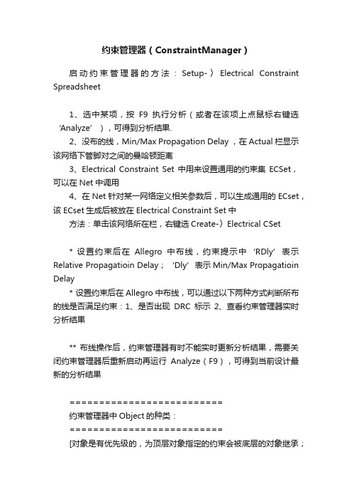
约束管理器(ConstraintManager)启动约束管理器的方法:Setup-〉Electrical Constraint Spreadsheet1、选中某项,按F9执行分析(或者在该项上点鼠标右键选‘Analyze’),可得到分析结果.2、没布的线,Min/Max Propagation Delay ,在Actual栏显示该网络下管脚对之间的曼哈顿距离3、Electrical Constraint Set中用来设置通用的约束集ECSet,可以在Net中调用4、在Net针对某一网络定义相关参数后,可以生成通用的ECset,该ECset生成后被放在Electrical Constraint Set中方法:单击该网络所在栏,右键选Create-〉Electrical CSet* 设置约束后在Allegro中布线,约束提示中‘RDly’表示Relative Propagatioin Delay;‘Dly’表示Min/Max Propagatioin Delay* 设置约束后在Allegro中布线,可以通过以下两种方式判断所布的线是否满足约束:1、是否出现DRC标示2、查看约束管理器实时分析结果** 布线操作后,约束管理器有时不能实时更新分析结果,需要关闭约束管理器后重新启动再运行Analyze(F9),可得到当前设计最新的分析结果==========================约束管理器中Object的种类:==========================[对象是有优先级的,为顶层对象指定的约束会被底层的对象继承;为底层对象指定的约束优先级高于从上层继承的约束][层次关系:系统System-〉设计Design-〉总线Bus-〉差分对Diff-Pair-〉扩展网络Xnet/网络Net-〉匹配群组Match Group-〉管脚对Pin-Pair]1、管脚对:位于同一Net或Xnet上的一对管脚2、网络/扩展网络3、总线(Bus)是管脚对、网络或者扩展网络Xnet的集合。
multi 正则 -回复

multi 正则-回复正则表达式(Regular Expression)是一种用于描述字符串模式的工具。
它是由特定字符和操作符组成的表达式,可以用来匹配、搜索和替换文本中的特定字符串。
在本文中,我们将一步一步地介绍正则表达式的基本概念、语法和应用实例。
第一步:正则表达式的基础概念正则表达式由多个字符组成,这些字符可以是字母、数字、特殊字符或预定义的字符集合。
它们形成了一种模式,用来描述我们希望匹配的字符串的特征。
比如,我们可以使用正则表达式/[0-9]/来匹配任意一个数字字符。
第二步:正则表达式的基本语法正则表达式的基本语法包含了字符和操作符。
其中,字符可以表示具体的字符或字符范围,而操作符则用于对字符进行匹配、重复和组合。
(1)字符:正则表达式中的字符可以是字母、数字或特殊字符。
比如,字符a表示匹配字符"a"本身,字符\d表示匹配任意一个数字字符。
(2)操作符:正则表达式中的操作符可以用于匹配、重复和组合字符。
常见的操作符包括:- 点(.):匹配任意一个字符,除了换行符。
- 星号(*):匹配前面的字符0次或多次。
- 加号(+):匹配前面的字符1次或多次。
- 问号(?):匹配前面的字符0次或1次。
- 花括号({}):匹配前面的字符指定的次数。
比如,{3}表示匹配前面的字符3次。
第三步:正则表达式的应用实例正则表达式可以应用于各种场景,比如数据验证、文本搜索和替换等。
下面我们将以实际应用的形式介绍正则表达式的用法。
(1)数据验证:正则表达式可以用于验证用户输入的数据是否符合特定的格式要求。
比如,我们可以使用正则表达式/^[A-Za-z0-9]{6,12}/来验证用户输入的密码是否由6到12个字母或数字组成。
(2)文本搜索:正则表达式可以用于在文本中查找特定的字符串。
比如,我们可以使用正则表达式/\b[A-Za-z]+\b/来匹配一个单词。
(3)文本替换:正则表达式可以用于替换文本中的特定字符串。
multi 正则 -回复

multi 正则-回复什么是正则表达式?正则表达式(Regular Expression,简称Regex)是一种用于模式匹配和文本处理的表达式。
它使用特定的符号和语法规则,可以用来匹配字符串中特定的模式,并对其进行查找、替换、拆分等操作。
正则表达式在文本处理、数据抽取、数据格式校验等各个领域都有广泛的应用。
为什么要使用正则表达式?正则表达式的使用可简化许多繁琐的文本处理任务。
通常情况下,我们需要处理的文本数据非常庞大,手动查找和处理是一项费时费力的工作。
而正则表达式可以通过一些简单的模式规则,快速定位到需要的文本,减少了人工操作的复杂性和错误率。
正则表达式的基本语法规则正则表达式由普通字符和特殊字符组成。
普通字符可以直接匹配输入文本中的相应字符。
而特殊字符则具有特定的含义,用于指定一些常见的匹配规则。
1. 匹配普通字符:正则表达式中的普通字符可以单个匹配文本中的相应字符。
例如,正则表达式cat 可以匹配文本中的"cat" 这个字符串。
2. 匹配元字符:元字符(Metacharacter)是正则表达式中具有特殊含义的字符。
常见的元字符包括. ^ * + ? { } [ ] \ ( )。
例如,正则表达式c.t 可以匹配"cat"、"cut" 等字符串;正则表达式^cat 可以匹配以"cat" 开头的字符串;正则表达式[abc] 可以匹配包含a、b 或c 的字符串。
3. 匹配字符集合:正则表达式中的方括号[] 用于指定一个字符集合。
字符集合可以包含多个字符,也可以使用连字符(-) 来表示一个字符范围。
例如,正则表达式[a-z] 可以匹配任意小写字母,正则表达式[0-9] 可以匹配任意数字。
4. 匹配量词:正则表达式中的量词用于指定匹配某个字符或模式的次数。
常见的量词包括*(匹配零次或多次)、+(匹配一次或多次)、?(匹配零次或一次)、{n}(匹配n 次)、{n,}(匹配至少n 次)、{n,m}(匹配至少n 次但不超过m 次)。
MUL、IMUL、DIV

MUL、IMUL、DIV大家好,今天这节课中我们来深入的学习下乘法指令。
乘法指令有两种,一种是有符号整数乘法另一种是无符号整数乘法,今天我们来学习无符号整数乘法。
MUL是进行无符号乘法的指令。
MUL(无符号乘法)指令有三种格式:第一种是将8位的操作数于al相乘。
第二种是将16位的操作数与ax相乘; 第三种是将32位的操作数与eax进行相乘乘数和被乘数大小必须相同,乘积的尺寸是乘数/被乘数大小的两倍。
三种格式都既接受寄存器操作数,也接受内存操作数。
但是不接受立即操作数(这点大家注意下)。
例如:你想将al寄存器中的值乘上2,那么此时你需要将立即数2存放到一个寄存器中,然后通过mul指令相乘,或者将立即数放到一个内存地址中,然后通过内存单元的形式来进行相乘。
举例:mov bl, 2mul bl ;此刻将bl寄存器中的值乘上al寄存器中的值指令中唯一的一个操作数是乘数。
也就是当我们的乘数是8位的时候,则与al相乘,如果我们的乘数是16位则与ax相乘,如果我们的乘数是32位则与eax寄存器相乘。
那么下面我给出mul乘法的相关操作数的实例被乘数乘数积al 8位操作数 axax 16位操作数 dx:axeax 32位操作数 edx:eax因为如果我们的乘数是一个8位操作数的话,我们的结果存在在ax寄存器中。
如果是16位操作数的话,我们的结果存放在dx:ax中。
如果dx不为0,则进位标志置位。
在执行完mul指令后,我们一般要检查下进位标志。
因为我们需要知道乘积的高半部分是否可以安全的忽略。
例如:mov al, 6hmov bl, 10hmul bl此刻我们检查进位标志cf = 0, 那么ah我们就可以将其忽略了,所以结果是60h。
那么我们再来举一个例子:例如:mov ax, 6000mov bx, 5000mul bx我们检查进位标志,此时cf = 1。
那么我们的结果是dx:ax ,此时我们的dx = 1E00, ax = 0000 所以最后我们的积为 1E000000。
ogg 外键约束

ogg 外键约束【实用版】目录1.OGG 外键约束的定义2.OGG 外键约束的作用3.OGG 外键约束的实现方式4.OGG 外键约束的优点与不足5.OGG 外键约束的实际应用案例正文1.OGG 外键约束的定义OGG(Object-Relational Mapping,对象关系映射)是一种数据库映射技术,用于将面向对象的编程语言与关系型数据库相结合。
在 OGG 中,外键约束是一种用于建立实体之间关联关系的机制。
它允许一个实体(称为“子实体”)通过外键与另一个实体(称为“父实体”)建立关联。
外键约束可以确保数据的完整性和一致性。
2.OGG 外键约束的作用OGG 外键约束在数据库设计中具有重要作用,主要表现在以下几点:(1)数据完整性:外键约束可以确保数据的完整性。
如果子实体与父实体之间存在关联,那么在插入或删除子实体记录时,需要确保父实体的存在。
这样可以避免数据孤立记录的产生,确保数据的一致性。
(2)数据关联:外键约束可以方便地实现实体之间的关联。
通过建立外键约束,可以方便地在查询时获取相关实体的信息,提高查询效率。
(3)数据安全性:外键约束可以提高数据的安全性。
通过设置外键约束,可以防止非法数据的插入和删除,确保数据的安全。
3.OGG 外键约束的实现方式在 OGG 中,实现外键约束的方式主要有以下几种:(1)在实体类中定义外键属性:在子实体的类中,可以定义一个外键属性,该属性关联到父实体的主键属性。
这样,在插入或删除子实体记录时,可以通过检查外键属性的值来确保父实体的存在。
(2)使用数据库约束:在数据库层面,可以设置外键约束。
这样,在插入或删除子实体记录时,数据库会自动检查外键约束,确保数据的完整性。
4.OGG 外键约束的优点与不足OGG 外键约束具有以下优点:(1)数据一致性:外键约束可以确保数据的一致性,避免数据孤立记录的产生。
(2)数据安全性:外键约束可以提高数据的安全性,防止非法数据的插入和删除。
- 1、下载文档前请自行甄别文档内容的完整性,平台不提供额外的编辑、内容补充、找答案等附加服务。
- 2、"仅部分预览"的文档,不可在线预览部分如存在完整性等问题,可反馈申请退款(可完整预览的文档不适用该条件!)。
- 3、如文档侵犯您的权益,请联系客服反馈,我们会尽快为您处理(人工客服工作时间:9:00-18:30)。
Multiple Regression by Iterative Fitting(EDTTS, Ch.7) We can use the same principle with more variables:(1a) Fit y using x1(2a) Fit residuals from step (1a) to x2(1b) Fit residuals from step (2a) to x1(2b) Fit residuals from step (1b) to x2(1c) Fit residuals from step (2b) to x1(2c) Fit residuals from step (1c) to x2and so on, until the coefficients are effectively zero.When fitting by least squares, the final residuals will be the same as the least squares residuals.Final coefficients must be calculated:Intercept: add intercept terms together from all regressions for x1:add coefficients of x1from (1a), (2a), (3a), ...for x2:add coefficients of x2from (1b), (2b), (3b), ... NB:This is a very slow way to obtain least squares fitA more direct way of finding this least squares fit that does not require iteration is to adjust each variable for the suc-cessive ones as described in EDTTS (Ch.7).We use this same "adjusted iterative fitting" when we replace the LS fit by the RR fit.Multiple Regression by Adjusted Iterative Fitting "Sweep out" one variable at a timeBasic idea:(1) Adjust y for x1→y⋅1(2) Adjust x2for x1→x2⋅1(3) Adjust y⋅1for x2⋅1Now y is adjusted for both x1and x2.Also, see how much of x1is in x2.See how this results in LS line:(1) Fit y to x1and form residuals:ˆy=c0+c1x1y⋅1=y−c1x1c1=ni=1Σ(x i1−x1)y i/ni=1Σ(x i1−x1)2(2) Fit x2to x1and form residuals:ˆx2=d0+d1x1x2⋅1=x2−d1x1d1=ni=1Σ(x i1−x1)x i2/ni=1Σ(x i1−x1)2(3) Fit y⋅1to x2⋅1and form residuals:ˆy⋅1=c0+c2x2⋅1y⋅12=y⋅1−c2x2⋅1c2=ni=1Σ(x2⋅1,i−x2⋅1)y⋅1,i/ni=1Σ(x2⋅1,i−x2⋅1)2Least squares fit isˆy=b0+b1x1+b2x2,whereb2=c2b1=c1−d1c2b0=mean(y i−b1x i1−b2x i2).Note:If you plot y⋅12against x1,the least squares slope of the line will be zero; likewise for x2.Everywhere above,replace "LS fit" with "RR line fit", but the "Note"no longer applies, so must add iterative steps: (4) Plot y⋅12against x1.If slope is not "small", adjust c1slope accordingly,forming new c1,y⋅1,c2,y⋅12. (5) Plot y⋅12against x2.If slope is not "small", adjust c1slope accordingly,return to (4).Otherwise, go to (6).(6) Obtainfinal residuals from step (5);obtain final fit from either(data−residuals)or from assembling all coefficients from all stepsor fromˆy=b0+b1+x1+b2x2whereb2=c2b1=c1−d1c2b0=median(y1−b1x i1−b2x i2).EDTTS, p.251: adjusted iterative fitting:(1) Fit y to x1=Poverty:y=87.54+1. 72x1+y⋅1(2) Fit x4=Infant mortality rate to x1:x4=89.82+1. 15x1+x4⋅1(3) Fit y⋅1to x4⋅1:y⋅1=−4. 34−0. 329x4⋅1+y⋅14 Assemble:y=87.54+1. 72x1−4. 34−0. 329(x4−89.82−1. 15x1)+y⋅14 =11 2.75+2. 10x1−0. 329x4+y⋅14Note:The correlation between x1and x4is high -- 0.57 --so unadjusted least squares fitting requires nine steps to converge to the least squares solution!(When the correla-tion is only 0.30, as for x1and x2,only six steps are needed.) We reduce the need for extensive iteration by adjusting variables as we go along.Same decomposition as before:data=fit1+residual1=fit2+residual2=fit3+residual3with final decompositiondata=(fit1+fit2+fit3)+residual3Here,fit2is obtained by fitting x2.1to residual1,and so on, as variables are used in turn.The results are not the same as fitting x2to residual1,unless x1is uncorrelated with x2 (there is no component of x1in x2).General procedure, > 2 independent variables:(1) Fit y to x1→y=c10+c1x1+y⋅1(2) Fit x2to x1→x2=d20+d21x1+x2⋅1(1) + (2)→(3):(3) Fit y⋅1to x2⋅1→y⋅1=c21+c2x2⋅1+y⋅12(4) Fit x3to x1and x2⋅1→x3=d30+d31x1+d32x2⋅1+x3⋅12(3) + (4)→(5)(5) Fit y⋅12to x3⋅12→y⋅12=c30+c3x3⋅12+y⋅123(6) Fit x4to x1,x2⋅1,x3⋅12→x4=d40+d41x1+d42x2⋅1+d43x3⋅12+x4⋅123(5) + (6)→(7):(7) Fit y⋅123to x4⋅123→y⋅123=c40+c4x4⋅123+y⋅1234(8) Fit x5to x1,x2⋅1,x3⋅12,x4⋅123→(etc.)Assemble coefficients (for intercepts,x1,x2,etc.)Strategies for removing variables:(1) Plot y versus x k,in turn; choose that x k for whichrelationship looks strongest.Note: some plots maysuggest transforming x kfirst; e.g.,1/income,log(rate).(2) Regress (rank of y i)on(rank of x ik), and choose thatx k for which the slope coefficient is largest (use ofranks reduces impact of outliers on the LS regression-- but there could be many ties for the "most signifi-cant" if there are only few data points and severalvariables have monotonic relationships with y)Some important facts to remember:(1) Thefit depends on what variables are in the equation.Omission of a variable can make drastic changes infit -- even rev e rse sign of coefficients(cf. fit of y⋅some to x k⋅some).(2) The LS coefficient b k can be obtained by regressingy⋅(all but k)on x k⋅(all but k).So a plot of y⋅(all but k)onx k⋅(all but k)is more informative than y on x k.Robust Regression: "Iteratively reweighted LS"y=Xβ+epislon=fit+roughˆβ=(X′X)−1X′ylinear function of y=(y1,... ,y n)′Weighted least squares:ˆβ=(X′WX)−1X′WyWWeight matrix W=diag(w1,...,w n)w i=BIG if residual is small(point i is "consistent" with "model")w i=little if resid-ual is large(point i is "inconsistent" with "model")Deciding on BIG and little residuals:•s_r=measure of spread of residuals (e.g., ...)•BIG residual if|resid|>6⋅s_r:w i=[1−(resid/6s2_r)]2|resid|<6s r(*)=0otherwiseIteratively re-weighted LS:1. Fit OLS→ˆβ(0)→r(0)=y−Xˆβ(0)2Calculate W(1 )[i,i]using r(0)i for resid for w i(*)3. Fitˆβvia WLS (weighted LS):→ˆβ(1 )→r(1 )=y−Xˆβ(1 )4Calculate W(2 )[i,i]using r(1 )i for resid for w i5. Fitˆβvia WLS using W(2 ):→ˆβ(2 )→r(2 )=y−Xˆβ(2 )|beta(k+1)−ˆβ(k)|<τ(tolerance)Iterate untilˆNotes:1. Starting with OLS is NOT robust, but it’s easy.2. Eqn(*) is called bisquare weight function:w i=1when residual=0w i=0when |residual|>6s_rfalls smoothly to zero3. The value "6" is a "tuning parameter"monly4≤c≤6.4. Any weight function that smoothly falls to zeroyields robust estimate ofβ.Biweight regression isespecially efficient.5. Easy to do computationally.See rlm(MASS):rlm(formula, data, weights, ..., subset, na.action,method = c("M", "MM", "model.frame"), ...)rlm(x, y,weights, w = rep(1, nrow(x)), init = "ls",-10-psi = psi.huber,method = c("M", "MM"), ... )method: currently either M-estimation or MM-estimationor (for the ’formula’ method only) find the model frame. MM-estimation is M-estimation with Tukey’s biweight initialized by a specific S-estimator.See ’Details’Psi functions are supplied for the Huber,Hampel and Tukey bisquare proposals as ’psi.huber’, ’psi.hampel’, ‘psi.bisquare’. Selecting ’method = "MM"’ selects a specific set of options which ensures that the estimator has a high breakdown point. The initial set of coefficients and the final scale are selected by an S-estimator with ’k0 = 1.548’; this gives(for n >> p) breakdown point 0.5. The final estimator isan M-estimator with Tukey’s biweight and fixed scale that will inherit this breakdown point provided ’c > k0’; thisis true for the default value of ’c’ that corresponds to95% relative efficiency at the normal.Case weights arenot supported for ’method = "MM"’.。