HHU Soil Mechanics Chapter 2 Permeability of Soil
二维水动力学模型糙率的推导和验证
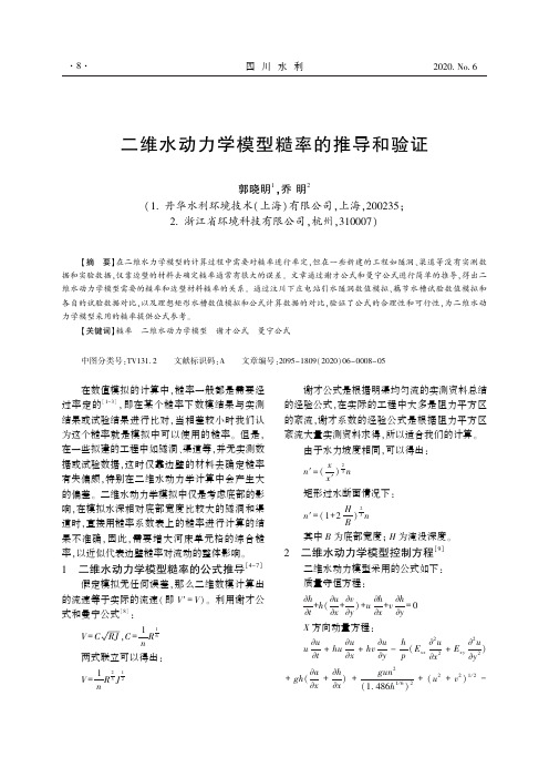
故水位即水深 H ) ,对矩形槽进行模拟。 计算中
2020 No 6
· 11·
四 川 水 利
E 取 2000Pa / s。
n′ = (1 + 2
H 2
)3n
B
代入 H = 6 37m、11 09m、15 62m。 可以得出
图 8 网格及平面示意
V=
1 2 1 1 BH 2 1
R3 J2 = (
) 3 J 2 Q = AV = BHV
n
n B + 2H
通过试算,可以得出三个流量对应的水深 H
分别 为 6 37m、 11 09m、 15 62m, 流 速 V 分 别 为
1 57m / s、1 804m / s、1 92m / s。 上 游 进 口 处 给 定
[ J] .长江科学院院报,2016,33(6) :29-35.
〔8〕 周 毅.基于 GIS 的溃坝洪水模拟与方法研究[ D] .
■
( 上接第 11 页)
的率定。 我们可以通过查糙率表,通过公式计算
( c) 流量 200m3 / s 时流速沿程变化 ( d) 流量 200m3 / s 时水位沿程变化
( e) 流量 300m3 / s 时流速沿程变化 ( f) 流量 300m3 / s 时水位沿程变化
据或试验数据,这时仅靠边壁的材料去确定糙率
有失偏颇,特别在二维水动力学计算中会产生大
n′ = (
的偏差。 二维水动力学模拟中仅是考虑底部的影
矩形过水断面情况下:
响,在模拟水深相对底部宽度比较大的隧洞和渠
n′ = (1 + 2
道时,直接用糙率系数表上的糙率进行计算的结
岩土工程专业英语词汇1
岩土工程专业英语词汇岩土工程专业英语词汇一. 综合类综合类 1.geotechnical engineering 岩土工程岩土工程 2.foundation engineering 基础工程基础工程3.soil, earth 土4.soil mechanics 土力学土力学 cyclic loading 周期荷载周期荷载 unloading 卸载卸载 reloading 再加载再加载 viscoelastic foundation 粘弹性地基粘弹性地基 viscous damping 粘滞阻尼粘滞阻尼 shear modulus 剪切模量剪切模量5.soil dynamics 土动力学土动力学6.stress path 应力路径应力路径二. 土的分类土的分类1.residual soil 残积土残积土 groundwater level 地下水位地下水位2.groundwater 地下水地下水groundwater table 地下水位地下水位 3.clay minerals 粘土矿物粘土矿物 4.secondary minerals 次生矿物次生矿物ndslides 滑坡滑坡 7.engineering geologic investigation 工程地质勘察工程地质勘察 8.boulder 漂石漂石9.cobble 卵石卵石 10.gravel 砂石砂石 11.gravelly sand 砾砂砾砂 12.coarse sand 粗砂粗砂 13.medium sand 中砂中砂14.fine sand 细砂细砂 15.silty sand 粉土粉土 16.clayey soil 粘性土粘性土 17.clay 粘土粘土 18.silty clay 粉质粘土粉质粘土19.silt 粉土粉土 20.sandy silt 砂质粉土砂质粉土 22.saturated soil 饱和土饱和土 23.unsaturated soil 非饱和土非饱和土 24.fill (soil)填土填土 29.soft clay 软粘土软粘土 30.expansive (swelling) soil 膨胀土31.peat 泥炭泥炭32.loess 黄土黄土 33.frozen soil 冻土冻土三. 土的基本物理力学性质土的基本物理力学性质24.degree of saturation 饱和度饱和度 25.dry unit weight 干重度干重度 26.moist unit weight 湿重度湿重度27.saturated unit weight 饱和重度饱和重度 28.effective unit weight 有效重度有效重度 29.density 密度密度pactness 密实度密实度 31.maximum dry density 最大干密度最大干密度32.optimum water content 最优含水量最优含水量 33.three phase diagram 三相图三相图34.tri-phase soil 三相土三相土 35.soil fraction 粒组粒组 36.sieve analysis 筛分筛分37.hydrometer analysis 比重计分析比重计分析 38.uniformity coefficient 不均匀系数不均匀系数39.coefficient of gradation 级配系数级配系数 40.fine-grained soil(silty and clayey)细粒土细粒土41.coarse- grained soil(gravelly and sandy)粗粒土粗粒土 42.Unified soil classification system 土的统一分类系统土的统一分类系统43.ASCE=American Society of Civil Engineer 美国土木工程师学会美国土木工程师学会44.AASHTO= American Association State Highway Officials 美国州公路官员协会美国州公路官员协会45.ISSMGE=International Society for Soil Mechanics and Geotechnical Engineering 国际土力学与岩土工程学会国际土力学与岩土工程学会 四. 渗透性和渗流渗透性和渗流1.Darcy ’s law 达西定律达西定律2.piping 管涌管涌3.flowing soil 流土流土4.sand boiling 砂沸砂沸5.flow net 流网流网6.seepage 渗透(流)渗透(流)7.leakage 渗流渗流8.seepage pressure 渗透压力渗透压力9.permeability 渗透性渗透性 10.seepage force 渗透力渗透力 11.hydraulic gradient 水力梯度水力梯度12.coefficient of permeability 渗透系数渗透系数五. 地基应力和变形地基应力和变形1.soft soil 软土软土2.(negative) skin friction of driven pile 打入桩(负)摩阻力打入桩(负)摩阻力3.effective stress 有效应力有效应力4.total stress 总应力总应力5.field vane shear strength 十字板抗剪强度十字板抗剪强度6.low activity 低活性低活性7.sensitivity 灵敏度灵敏度8.triaxial test 三轴试验三轴试验9.foundation design 基础设计基础设计10.recompaction 再压缩再压缩 11.bearing capacity 承载力承载力 12.soil mass 土体土体13.contact stress (pressure)接触应力(压力)接触应力(压力) 14.concentrated load 集中荷载集中荷载 15.a semi-infinite elastic solid 半无限弹性体半无限弹性体 16.homogeneous 均质均质 17.isotropi 17.isotropic c 各向同性各向同性18.strip footing 条基条基 19.square spread footing 方形独立基础方形独立基础20.underlying soil (stratum ,strata)下卧层(土)下卧层(土) 21.dead load =sustained load 恒载恒载 持续荷载持续荷载22.live load 活载活载 23.short –term transient load 短期瞬时荷载短期瞬时荷载24.long-term transient load 长期荷载长期荷载 26.settlement 沉降沉降 27.deformation 变形变形 28.casing 套管套管 29.dike=dyke 堤(防)堤(防) 30.clay fraction 粘粒粒组粘粒粒组32.subgrade 路基路基 33.well-graded soil 级配良好土级配良好土 34.poorly-graded soil 级配不良土级配不良土35.normal stresses 正应力正应力 36.shear stresses 剪应力剪应力 37.principal plane 主平面主平面38.major (intermediate, minor) principal stress 最大(中、最小)主应力最大(中、最小)主应力39.Mohr-Coulomb failure condition 摩尔-库仑破坏条件库仑破坏条件42.pore water pressure 孔隙水压力孔隙水压力 43.preconsolidation pressure 先期固结压力先期固结压力44.modulus of compressibility 压缩模量压缩模量 45.coefficent of compressibility 压缩系数压缩系数pression index 压缩指数压缩指数 47.swelling index 回弹指数回弹指数48.geostatic stress 自重应力自重应力 49.additional stress 附加应力附加应力 50.total stress 总应力总应力51.final settlement 最终沉降最终沉降 52.slip line 滑动线滑动线六. 基坑开挖与降水基坑开挖与降水1 excavation 开挖(挖方)开挖(挖方)2 dewatering (基坑)降水(基坑)降水3 failure of foundation 基坑失稳基坑失稳4 bracing of foundation pit 基坑围护基坑围护5 bottom heave=basal heave (基坑)底隆起(基坑)底隆起6 retaining wall 挡土墙挡土墙7 pore-pressure distribution 孔压分布孔压分布8 dewatering method 降低地下水位法降低地下水位法 9 well point system 井点系统(轻型)井点系统(轻型) 10 deep well point 深井点深井点 11 vacuum well point 真空井点真空井点 12 braced cuts 支撑围护支撑围护 13 braced excavation 支撑开挖支撑开挖 14 braced sheeting 支撑挡板支撑挡板七. 深基础--deep foundation1.pile foundation 桩基础桩基础 1)cast –in-place 灌注桩灌注桩 diving casting cast-in-place pile 沉管灌注桩沉管灌注桩 bored pile 钻孔桩钻孔桩 piles set into rock 嵌岩灌注桩嵌岩灌注桩 rammed bulb pile 夯扩桩夯扩桩2)belled pier foundation 钻孔墩基础钻孔墩基础 drilled-pier foundation 钻孔扩底墩钻孔扩底墩3)precast concrete pile 预制混凝土桩预制混凝土桩4)steel pile 钢桩钢桩 steel pipe pile 钢管桩钢管桩 steel sheet pile 钢板桩钢板桩5)prestressed concrete pile 预应力混凝土桩预应力混凝土桩 prestressed concrete pipe pile 预应力混凝土管桩预应力混凝土管桩2.caisson foundation 沉井(箱)沉井(箱)3.diaphram wall 地下连续墙地下连续墙 截水墙截水墙4.friction pile 摩擦桩摩擦桩5.end-bearing pile 端承桩端承桩6.shaft 竖井;桩身竖井;桩身 8.pile caps 承台(桩帽)承台(桩帽)9.bearing capacity of single pile 单桩承载力单桩承载力 teral pile load test 单桩横向载荷试验单桩横向载荷试验 11.ultimate lateral resistance of single pile 单桩横向极限承载力单桩横向极限承载力13.vertical allowable load capacity 单桩竖向容许承载力单桩竖向容许承载力14.low pile cap 低桩承台低桩承台 15.high-rise pile cap 高桩承台高桩承台16.vertical ultimate uplift resistance of single pile 单桩抗拔极限承载力单桩抗拔极限承载力17.silent piling 静力压桩静力压桩 18.uplift pile 抗拔桩抗拔桩 19.anti-slide pile 抗滑桩抗滑桩20.pile groups 群桩群桩21.efficiency factor of pile groups 群桩效率系数(η) 22.efficiency of pile groups 群桩效应群桩效应 23.dynamic pile testing 桩基动测技术桩基动测技术24.final set 最后贯入度最后贯入度 27.pile head=butt 桩头桩头 28.pile tip=pile point=pile toe 桩端(头)桩端(头)29.pile spacing 桩距桩距 30.pile plan 桩位布置图桩位布置图 31.arrangement of piles =pile layout 桩的布置桩的布置32.group action 群桩作用群桩作用 33.end bearing=tip resistance 桩端阻桩端阻34.skin(side) friction=shaft resistance 桩侧阻桩侧阻 35.pile cushion 桩垫桩垫 36.pile driving(by vibration) (振动)打桩(振动)打桩 37.pile pulling test 拔桩试验拔桩试验 38.pile shoe 桩靴桩靴 八. 地基处理--ground treatment2.cushion 垫层法垫层法3.preloading 预压法预压法4.dynamic compaction 强夯法强夯法5.dynamic compaction replacement 强夯置换法强夯置换法6.vibroflotation method 振冲法振冲法7.sand-gravel pile 砂石桩砂石桩 8.gravel pile(stone column)碎石桩碎石桩9.cement-flyash-gravel pile(CFG)水泥粉煤灰碎石桩水泥粉煤灰碎石桩 10.cement mixing method 水泥土搅拌桩水泥土搅拌桩 11.cement column 水泥桩水泥桩 12.lime pile (lime column)石灰桩石灰桩 13.jet grouting 高压喷射注浆法高压喷射注浆法14.rammed-cement-soil pile 夯实水泥土桩法夯实水泥土桩法 15.lime-soil compaction pile 灰土挤密桩灰土挤密桩 lime-soil compacted column 灰土挤密桩灰土挤密桩 lime soil pile 灰土挤密桩灰土挤密桩16.chemical stabilization 化学加固法化学加固法 17.surface compaction 表层压实法表层压实法18.surcharge preloading 超载预压法超载预压法 19.vacuum preloading 真空预压法真空预压法21.geofabric ,geotextile 土工织物土工织物 posite foundation 复合地基复合地基23.reinforcement method 加筋法加筋法 24.dewatering method 降低地下水固结法降低地下水固结法26.expansive ground treatment 膨胀土地基处理膨胀土地基处理27.ground treatment in mountain area 山区地基处理山区地基处理28.collapsible loess treatment 湿陷性黄土地基处理湿陷性黄土地基处理 29.artificial foundation 人工地基人工地基30.natural foundation 天然地基天然地基 31.pillow 褥垫褥垫 32.soft clay ground 软土地基软土地基 33.sand drain 砂井砂井 34.root pile 树根桩树根桩 35.plastic drain 塑料排水带塑料排水带九. 固结consolidation1.Terzzaghi ’s consolidation theory 太沙基固结理论太沙基固结理论2.Barraon ’s consolidation theory 巴隆固结理论巴隆固结理论3.Biot ’s consolidation theory 比奥固结理论比奥固结理论4.over consolidation ration (OCR)超固结比超固结比5.overconsolidation soil 超固结土超固结土6.excess pore water pressure 超孔压力超孔压力7.multi-dimensional consolidation 多维固结多维固结 8.one-dimensional consolidation 一维固结一维固结9.primary consolidation 主固结主固结 10.secondary consolidation 次固结次固结11.degree of consolidation 固结度固结度 15.coefficient of consolidation 固结系数固结系数16.preconsolidation pressure 前期固结压力前期固结压力 17.principle of effective stress 有效应力原理有效应力原理18.consolidation under K0 condition K0固结固结十. 抗剪强度shear strength1.undrained shear strength 不排水抗剪强2.residual strength 残余强度残余强度3.long-term strength 长期强度长期强度4.peak strength 峰值强度峰值强度5.shear strain rate 剪切应变速率剪切应变速率6.dilatation 剪胀剪胀7.effective stress approach of shear strength 剪胀抗剪强度有效应力法剪胀抗剪强度有效应力法8.total stress approach of shear strength 抗剪强度总应力法抗剪强度总应力法 9.Mohr-Coulomb theory 莫尔-库仑理论莫尔-库仑理论 10.angle of internal friction 内摩擦角内摩擦角11.cohesion 粘聚力粘聚力 12.failure criterion 破坏准则破坏准则13.vane strength 十字板抗剪强度十字板抗剪强度 14.unconfined compression 无侧限抗压强度无侧限抗压强度15.effective stress failure envelop 有效应力破坏包线有效应力破坏包线16.effective stress strength parameter 有效应力强度参数有效应力强度参数十一. 本构模型--constitutive model1.elastic model 弹性模型弹性模型2.nonlinear elastic model 非线性弹性模型非线性弹性模型3.elastoplastic model 弹塑性模型弹塑性模型4.viscoelastic model 粘弹性模型粘弹性模型5.boundary surface model 边界面模型边界面模型6.Duncan-Chang model 邓肯-张模型邓肯-张模型7.rigid plastic model 刚塑性模型刚塑性模型 8.cap model 盖帽模型盖帽模型 9.work softening 加工软化加工软化10.work hardening 加工硬化加工硬化 11.Cambridge model 剑桥模型剑桥模型 12.ideal elastoplastic model 理想弹塑性模型理想弹塑性模型13.Mohr-Coulomb yield criterion 莫尔-库仑屈服准则莫尔-库仑屈服准则 14.yield surface 屈服面屈服面15.elastic half-space foundation model 弹性半空间地基模型弹性半空间地基模型16.elastic modulus 弹性模量弹性模量 17.Winkler foundation model 文克尔地基模型文克尔地基模型 十二. 地基承载力--bearing capacity of foundation soil1.punching shear failure 冲剪破坏冲剪破坏2.general shear failure 整体剪切破化整体剪切破化3.local shear failure 局部剪切破坏局部剪切破坏4.state of limit equilibrium 极限平衡状态极限平衡状态5.critical edge pressure 临塑荷载临塑荷载6.stability of foundation soil 地基稳定性地基稳定性7.ultimate bearing capacity of foundation soil 地基极限承载力地基极限承载力8.allowable bearing capacity of foundation soil 地基容许承载力地基容许承载力十三. 土压力--earth pressure1.active earth pressure 主动土压力主动土压力2.passive earth pressure 被动土压力被动土压力3.earth pressure at rest 静止土压力静止土压力4.Coulomb ’s earth pressure theory 库仑土压力理论库仑土压力理论5.Rankine ’s earth pressure theory 朗金土压力理论朗金土压力理论十四. 土坡稳定分析--slope stability analysis1.angle of repose 休止角休止角 3.safety factor of slope 边坡稳定安全系数边坡稳定安全系数5.Swedish circle method 瑞典圆弧滑动法瑞典圆弧滑动法6.slices method 条分法条分法十五. 挡土墙--retaining wall1.stability of retaining wall 挡土墙稳定性挡土墙稳定性2.foundation wall 基础墙基础墙3.counter retaining wall 扶壁式挡土墙扶壁式挡土墙4.cantilever retaining wall 悬臂式挡土墙悬臂式挡土墙5.cantilever sheet pile wall 悬臂式板桩墙悬臂式板桩墙6.gravity retaining wall 重力式挡土墙重力式挡土墙7.anchored plate retaining wall 锚定板挡土墙锚定板挡土墙 8.anchored sheet pile wall 锚定板板桩墙锚定板板桩墙 十六. 板桩结构物--sheet pile structure1.steel sheet pile 钢板桩钢板桩2.reinforced concrete sheet pile 钢筋混凝土板桩钢筋混凝土板桩3.steel piles 钢桩钢桩4.wooden sheet pile 木板桩木板桩5.timber piles 木桩木桩十七. 浅基础--shallow foundation1.box foundation 箱型基础箱型基础2.mat(raft) foundation 片筏基础片筏基础3.strip foundation 条形基础条形基础4.spread footing 扩展基础扩展基础pensated foundation 补偿性基础补偿性基础6.bearing stratum 持力层持力层7.rigid foundation 刚性基础刚性基础 8.flexible foundation 柔性基础柔性基础9.embedded depth of foundation 基础埋置深度基础埋置深度 foundation pressure 基底附加应力基底附加应力11.structure-foundation-soil interaction analysis 上部结构-基础-地基共同作用分析上部结构-基础-地基共同作用分析 十八. 土的动力性质--dynamic properties of soils1.dynamic strength of soils 动强度动强度2.wave velocity method 波速法波速法3.material damping 材料阻尼材料阻尼4.geometric damping 几何阻尼几何阻尼5.damping ratio 阻尼比阻尼比6.initial liquefaction 初始液化初始液化7.natural period of soil site 地基固有周期地基固有周期8.dynamic shear modulus of soils 动剪切模量动剪切模量 9.dynamic magnification factor 动力放大因素动力放大因素10.liquefaction strength 抗液化强度抗液化强度 11.dimensionless frequency 无量纲频率无量纲频率12.evaluation of liquefaction 液化势评价液化势评价 13.stress wave in soils 土中应力波土中应力波14.dynamic settlement 振陷(动沉降)振陷(动沉降)十九. 动力机器基础动力机器基础1.equivalent lumped parameter method 等效集总参数法等效集总参数法2.dynamic subgrade reaction method 动基床反力法动基床反力法3.vibration isolation 隔振隔振4.foundation vibration 基础振动基础振动5.elastic half-space theory of foundation vibration 基础振动弹性半空间理论基础振动弹性半空间理论6.allowable amplitude of foundation 基础振动容许振幅基础振动容许振幅7.natural frequency of foundation 基础自振频率基础自振频率二十. 地基基础抗震地基基础抗震1.earthquake engineering 地震工程地震工程2.soil dynamics 土动力学土动力学3.duration of earthquake 地震持续时间地震持续时间4.earthquake response spectrum 地震反应谱地震反应谱5.earthquake intensity 地震烈度地震烈度6.earthquake magnitude 震级震级7.seismic predominant period 地震卓越周期地震卓越周期8.maximum acceleration of earthquake 地震最大加速度地震最大加速度二十一. 室内土工实验室内土工实验1.high pressure consolidation test 高压固结试验高压固结试验2.consolidation under K0 condition K0固结试验固结试验3.falling head permeability 变水头试验变水头试验4.constant head permeability 常水头渗透试验常水头渗透试验5.unconsolidated-undrained triaxial test 不固结不排水试验(UU)6.consolidated undrained triaxial test 固结不排水试验(CU)7.consolidated drained triaxial test 固结排水试验(CD) paction test 击实试验击实试验9.consolidated quick direct shear test 固结快剪试验固结快剪试验 10.quick direct shear test 快剪试验快剪试验11.consolidated drained direct shear test 慢剪试验慢剪试验 12.sieve analysis 筛分析筛分析 13.geotechnical model test 土工模型试验土工模型试验 14.centrifugal model test 离心模型试验离心模型试验15.direct shear apparatus 直剪仪直剪仪 16.direct shear test 直剪试验直剪试验17.direct simple shear test 直接单剪试验直接单剪试验 18.dynamic triaxial test 三轴试验三轴试验19.dynamic simple shear 动单剪动单剪 20.free (resonance )vibration column test 自(共)振柱试验振柱试验 二十二. 原位测试原位测试1.standard penetration test (SPT)标准贯入试验标准贯入试验2.surface wave test (SWT)表面波试验表面波试验3.dynamic penetration test(DPT)动力触探试验动力触探试验4.static cone penetration (SPT) 静力触探试验静力触探试验5.plate loading test 静力荷载试验静力荷载试验teral load test of pile 单桩横向载荷试验单桩横向载荷试验7.static load test of pile 单桩竖向荷载试验单桩竖向荷载试验 8.cross-hole test 跨孔试验跨孔试验9.screw plate test 螺旋板载荷试验螺旋板载荷试验 10.pressuremeter test 旁压试验旁压试验11.light sounding 轻便触探试验轻便触探试验 12.deep settlement measurement 深层沉降观测深层沉降观测13.vane shear test 十字板剪切试验十字板剪切试验 14.field permeability test 现场渗透试验现场渗透试验15.in-situ pore water pressure measurement 原位孔隙水压量测原位孔隙水压量测 16.in-situ soil test 原位试验原位试验。
2、渗流理论1

本章内容
第1节 地下水引发的工程问题
第2节 达西定律
第3节 流网理论简介 第4节 流土、管涌及其防治 第5节 非饱和土的湿化及其危害
ቤተ መጻሕፍቲ ባይዱ
第1节 地下水引发的工程问题
Soil mechanics Chapter 2 (WRH)
第2节 达西定律
水在土的孔隙中流动,其形式可以分为: 层流:水的流速很慢,认为相邻两个水分子运动轨 迹相互平行而不混掺。 紊流:紊流与层流的意义相反。
Soil mechanics Chapter 2 (WRH)
第二章 渗流、 渗流、流土和湿化
§2.1 地下水引发的工程问题 §2.2 达西定律 §2.3 流网理论简介 §2.4 流土、管涌及其防治 2.5非饱和土的湿化及其危害 §2.5
第1节 地下水引发的工程问题
Soil mechanics Chapter 2 (WRH)
地下水位≈ 地下水位≈测压管水面
不透水层 优点: 优点:可获得现场较为可 靠的平均渗透系数 缺点:费用较高,耗时较长 缺点:费用较高,
第1节 地下水引发的工程问题
Soil mechanics 第2节 达西定律 Chapter 2 (WRH)
4.层状地基的等效渗透系数 4.层状地基的等效渗透系数
三. 渗透系数的测定 测定土的渗透系数的方法有:
常水头试验法
室内试验测定方法
变水头试验法
野外试验测定方法
井孔抽水试验 井孔注水试验
第1节 地下水引发的工程问题
Soil mechanics 第2节 达西定律 Chapter 2 (WRH)
1.常水头渗透试验 1.常水头渗透试验
该试验适用于渗透性大的粗颗粒土。试验装置如图所示, 该试验适用于渗透性大的粗颗粒土。试验装置如图所示,圆 柱体试料断面积为A 长度为l 保持水头差h不变, 柱体试料断面积为A,长度为l,保持水头差h不变,测定经过 一定时间t的透水量是V 渗透系数k可根据式导出如下: 一定时间t的透水量是V,渗透系数k可根据式导出如下:
土力学电子教材-同济大学
在线练习开始页
土的物理性质及其工程分类 土中水的运动规律 土的应力分布及计算 土的压缩与地基沉降计算 土的抗剪强度 土压力计算 土坡稳定分析 地基承载力
/jpkc/soil/zice/Question.htm2013-5-27 8:51:10
课程习题开始页
土力学教学大纲
习题
(四)土的压缩性和固结理论
1.概述 2.土的压缩特性 3.土的固结状态 4.有效应力原理 5.太沙基一维固结理论 习题
(五)土中应力和地基沉降计算
1.概述 2.地基中的自重应力 3.地基中的附加应力 4.常用沉降计算方法 5.地基沉降随时间变化规律的分析 习题
/jpkc/soil/Dagang/Jxdg.htm(第 6/9 页)2013-5-27 8:51:23
土中水的运动规律
学习指导 工程背景 渗透理论
渗流模型 达西渗透定律 渗透系数的确定 流网及其工程应用
概述 流网的绘制 流网的应用 土中渗透作用力与渗透变形
渗透力 渗透变形 本章小结
/jpkc/soil/common/book.htm(第 2/7 页)2013-5-27 8:50:31
(七)地基承载力
1.了解地基破坏模式 2.掌握地基极限承载力的计算方法 掌握按极限平衡条件确定地基临塑荷载、塑性荷载、 极限荷载的方法;同时掌握规范确定地基承载力的方 法。
/jpkc/soil/Dagang/Jxdg.htm(第 3/9 页)2013-5-27 8:51:23
土中应力和地基沉降计算 土的抗剪强度
法,熟悉土的基本物理力学性质,掌握地基沉降、地 基承载力、土压力计算方法和土坡稳定分析方法,掌 握一般土工试验方法,达到能应用土力学的基本原理
地基承载力
yantubbs-The hardening soil model, Formulation and verification

The hardening soil model: Formulation and verificationT. SchanzLaboratory of Soil Mechanics, Bauhaus-University Weimar, GermanyP.A. VermeerInstitute of Geotechnical Engineering, University Stuttgart, GermanyP.G. BonnierP LAXIS B.V., NetherlandsKeywords: constitutive modeling, HS-model, calibration, verificationABSTRACT: A new constitutive model is introduced which is formulated in the framework of classical theory of plasticity. In the model the total strains are calculated using a stress-dependent stiffness, different for both virgin loading and un-/reloading. The plastic strains are calculated by introducing a multi-surface yield criterion. Hardening is assumed to be isotropic depending on both the plastic shear and volumetric strain. For the frictional hardening a non-associated and for the cap hardening an associated flow rule is assumed.First the model is written in its rate form. Therefor the essential equations for the stiffness mod-ules, the yield-, failure- and plastic potential surfaces are given.In the next part some remarks are given on the models incremental implementation in the P LAXIS computer code. The parameters used in the model are summarized, their physical interpre-tation and determination are explained in detail.The model is calibrated for a loose sand for which a lot of experimental data is available. With the so calibrated model undrained shear tests and pressuremeter tests are back-calculated.The paper ends with some remarks on the limitations of the model and an outlook on further de-velopments.1INTRODUCTIONDue to the considerable expense of soil testing, good quality input data for stress-strain relation-ships tend to be very limited. In many cases of daily geotechnical engineering one has good data on strength parameters but little or no data on stiffness parameters. In such a situation, it is no help to employ complex stress-strain models for calculating geotechnical boundary value problems. In-stead of using Hooke's single-stiffness model with linear elasticity in combination with an ideal plasticity according to Mohr-Coulomb a new constitutive formulation using a double-stiffness model for elasticity in combination with isotropic strain hardening is presented.Summarizing the existing double-stiffness models the most dominant type of model is the Cam-Clay model (Hashiguchi 1985, Hashiguchi 1993). To describe the non-linear stress-strain behav-iour of soils, beside the Cam-Clay model the pseudo-elastic (hypo-elastic) type of model has been developed. There an Hookean relationship is assumed between increments of stress and strain and non-linearity is achieved by means of varying Young's modulus. By far the best known model of this category ist the Duncan-Chang model, also known as the hyperbolic model (Duncan & Chang 1970). This model captures soil behaviour in a very tractable manner on the basis of only two stiff-ness parameters and is very much appreciated among consulting geotechnical engineers. The major inconsistency of this type of model which is the reason why it is not accepted by scientists is that, in contrast to the elasto-plastic type of model, a purely hypo-elastic model cannot consistently dis-tinguish between loading and unloading. In addition, the model is not suitable for collapse load computations in the fully plastic range.12These restrictions will be overcome by formulating a model in an elasto-plastic framework in this paper. Doing so the Hardening-Soil model, however, supersedes the Duncan-Chang model by far. Firstly by using the theory of plasticity rather than the theory of elasticity. Secondly by includ-ing soil dilatancy and thirdly by introducing a yield cap.In contrast to an elastic perfectly-plastic model, the yield surface of the Hardening Soil model is not fixed in principal stress space, but it can expand due to plastic straining. Distinction is made between two main types of hardening, namely shear hardening and compression hardening. Shear hardening is used to model irreversible strains due to primary deviatoric loading. Compression hardening is used to model irreversible plastic strains due to primary compression in oedometer loading and isotropic loading.For the sake of convenience, restriction is made in the following sections to triaxial loading conditions with 2σ′ = 3σ′ and 1σ′ being the effective major compressive stress.2 CONSTITUTIVE EQUATIONS FOR STANDARD DRAINED TRIAXIAL TESTA basic idea for the formulation of the Hardening-Soil model is the hyperbolic relationship be-tween the vertical strain ε1, and the deviatoric stress, q , in primary triaxial loading. When subjected to primary deviatoric loading, soil shows a decreasing stiffness and simultaneously irreversible plastic strains develop. In the special case of a drained triaxial test, the observed relationship be-tween the axial strain and the deviatoric stress can be well approximated by a hyperbola (Kondner& Zelasko 1963). Standard drained triaxial tests tend to yield curves that can be described by:The ultimate deviatoric stress, q f , and the quantity q a in Eq. 1 are defined as:The above relationship for q f is derived from the Mohr-Coulomb failure criterion, which involves the strength parameters c and ϕp . As soon as q = q f , the failure criterion is satisfied and perfectly plastic yielding occurs. The ratio between q f and q a is given by the failure ratio R f , which should obviously be smaller than 1. R f = 0.9 often is a suitable default setting. This hyperbolic relationship is plotted in Fig. 1.2.1 Stiffness for primary loadingThe stress strain behaviour for primary loading is highly nonlinear. The parameter E 50 is the con-fining stress dependent stiffness modulus for primary loading. E 50is used instead of the initial modulus E i for small strain which, as a tangent modulus, is more difficult to determine experimen-tally. It is given by the equation:ref E 50is a reference stiffness modulus corresponding to the reference stress ref p . The actual stiff-ness depends on the minor principal stress, 3σ′, which is the effective confining pressure in a tri-axial test. The amount of stress dependency is given by the power m . In order to simulate a loga-rithmic stress dependency, as observed for soft clays, the power should be taken equal to 1.0. As a3Figure 1. Hyperbolic stress-strain relation in primary loading for a standard drained triaxial test.secant modulus ref E 50 is determined from a triaxial stress-strain-curve for a mobilization of 50% ofthe maximum shear strength q f .2.2 Stiffness for un-/reloadingFor unloading and reloading stress paths, another stress-dependent stiffness modulus is used:where ref urE is the reference Young's modulus for unloading and reloading, corresponding to the reference pressure σ ref . Doing so the un-/reloading path is modeled as purely (non-linear) elastic.The elastic components of strain εe are calculated according to a Hookean type of elastic relation using Eqs. 4 + 5 and a constant value for the un-/reloading Poisson's ratio υur .For drained triaxial test stress paths with σ2 = σ3 = constant, the elastic Young's modulus E ur re-mains constant and the elastic strains are given by the equations:Here it should be realised that restriction is made to strains that develop during deviatoric loading,whilst the strains that develop during the very first stage of the test are not considered. For the first stage of isotropic compression (with consolidation), the Hardening-Soil model predicts fully elastic volume changes according to Hooke's law, but these strains are not included in Eq. 6.2.3 Yield surface, failure condition, hardening lawFor the triaxial case the two yield functions f 12 and f 13 are defined according to Eqs. 7 and 8. Here4Figure 2. Successive yield loci for various values of the hardening parameter γ p and failure surface.the measure of the plastic shear strain γ p according to Eq. 9 is used as the relevant parameter forthe frictional hardening:with the definitionIn reality, plastic volumetric strains p υε will never be precisely equal to zero, but for hard soils plastic volume changes tend to be small when compared with the axial strain, so that the approxi-mation in Eq. 9 will generally be accurate.For a given constant value of the hardening parameter, γ p , the yield condition f 12 = f 13 = 0 can be visualised in p'-q-plane by means of a yield locus. When plotting such yield loci, one has to use Eqs. 7 and 8 as well as Eqs. 3 and 4 for E 50 and E ur respectively. Because of the latter expressions,the shape of the yield loci depends on the exponent m . For m = 1.0 straight lines are obtained, but slightly curved yield loci correspond to lower values of the exponent. Fig. 2 shows the shape of successive yield loci for m = 0.5, being typical for hard soils. For increasing loading the failure sur-faces approach the linear failure condition according to Eq. 2.2.4 Flow rule, plastic potential functionsHaving presented a relationship for the plastic shear strain, γ p , attention is now focused on the plastic volumetric strain p υε. As for all plasticity models, the Hardening-Soil model involves a re-lationship between rates of plastic strain, i.e. a relationship between p υε and p γ . This flow rule hasthe linear form:5Clearly, further detail is needed by specifying the mobilized dilatancy angle m ψ. For the presentmodel, the expression:is adopted, where cv ϕ is the critical state friction angle, being a material constant independent ofdensity (Schanz & Vermeer 1996), and m ϕ is the mobilized friction angle:The above equations correspond to the well-known stress-dilatancy theory (Rowe 1962, Rowe 1971), as explained by (Schanz & Vermeer 1996). The essential property of the stress-dilatancy theory is that the material contracts for small stress ratios m ϕ < cv ϕ, whilst dilatancy occurs for high stress ratios m ϕ < cv ϕ. At failure, when the mobilized friction angle equals the failure angle,p ϕ, it is found from Eq. 11 that:Hence, the critical state angle can be computed from the failure angles p ϕand p ψ. The above defi-nition of the flow rule is equivalent to the definition of definition of the plastic potential functionsg 12 and g 13 according to:Using theKoiter-rule (Koiter 1960) for yielding depending on two yield surfaces (Multi-surface plasticity ) one finds:Calculating the different plastic strain rates by this equation, Eq. 10 directly follows.3 TIME INTEGRATIONThe model as described above has been implemented in the finite element code P LAXIS (Vermeer& Brinkgreve 1998). To do so, the model equations have to be written in incremental form. Due to this incremental formulation several assumptions and modifications have to be made, which will be explained in this section.During the global iteration process, the displacement increment follows from subsequent solu-tion of the global system of equations:where K is the global stiffness matrix in which we use the elastic Hooke's matrix D , f ext is a global load vector following from the external loads and f int is the global reaction vector following from the stresses. The stress at the end of an increment σ 1 can be calculated (for a given strain increment ∆ε) as:6whereσ0 , stress at the start of the increment,∆σ , resulting stress increment,4D , Hooke's elasticity matrix, based on the unloading-reloading stiffness,∆ε , strain increment (= B ∆u ),γ p , measure of the plastic shear strain, used as hardening parameter,∆Λ , increment of the non-negative multiplier,g , plastic potential function.The multiplier Λ has to be determined from the condition that the function f (σ1, γ p ) = 0 has to be zero for the new stress and deformation state.As during the increment of strain the stresses change, the stress dependant variables, like the elasticity matrix and the plastic potential function g , also change. The change in the stiffness during the increment is not very important as in many cases the deformations are dominated by plasticity.This is also the reason why a Hooke's matrix is used. We use the stiffness matrix 4D based on the stresses at the beginning of the step (Euler explicit ). In cases where the stress increment follows from elasticity alone, such as in unloading or reloading, we iterate on the average stiffness during the increment.The plastic potential function g also depends on the stresses and the mobilized dilation angle m ψ. The dilation angle for these derivatives is taken at the beginning of the step. The implementa-tion uses an implicit scheme for the derivatives of the plastic potential function g . The derivatives are taken at a predictor stress σtr , following from elasticity and the plastic deformation in the previ-ous iteration:The calculation of the stress increment can be performed in principal stress space. Therefore ini-tially the principal stresses and principal directions have to be calculated from the Cartesian stresses, based on the elastic prediction. To indicate this we use the subscripts 1, 2 and 3 and have 321σσσ≥≥ where compression is assumed to be positive.Principal plastic strain increments are now calculated and finally the Cartesian stresses have to be back-calculated from the resulting principal constitutive stresses. The calculation of the consti-tutive stresses can be written as:From this the deviatoric stress q (σ1 – σ3) and the asymptotic deviatoric stress q a can be expressed in the elastic prediction stresses and the multiplier ∆Λ:7whereFor these stresses the functionshould be zero. As the increment of the plastic shear strain ∆γ p also depends linearly on the multi-plier ∆Λ, the above formulae result in a (complicated) quadratic equation for the multiplier ∆Λwhich can be solved easily. Using the resulting value of ∆Λ, one can calculate (incremental)stresses and the (increment of the) plastic shear strain.In the above formulation it is assumed that there is a single yield function. In case of triaxial compression or triaxial extension states of stress there are two yield functions and two plastic po-tential functions. Following (Koiter 1960) one can write:where the subscripts indicate the principal stresses used for the yield and potential functions. At most two of the multipliers are positive. In case of triaxial compression we have σ2 = σ3, Λ23 = 0and we use two consistency conditions instead of one as above. The increment of the plastic shear strain has to be expressed in the multipliers. This again results in a quadratic equation in one of the multipliers.When the stresses are calculated one still has to check if the stress state violates the yield crite-rion q ≤ q f . When this happens the stresses have to be returned to the Mohr-Coulomb yield surface.4 ON THE CAP YIELD SURFACEShear yield surfaces as indicated in Fig. 2 do not explain the plastic volume strain that is measured in isotropic compression. A second type of yield surface must therefore be introduced to close the elastic region in the direction of the p-axis. Without such a cap type yield surface it would not be possible to formulate a model with independent input of both E 50 and E oed . The triaxial modulus largely controls the shear yield surface and the oedometer modulus controls the cap yield surface.In fact, ref E 50largely controls the magnitude of the plastic strains that are associated with the shear yield surface. Similarly, ref oedE is used to control the magnitude of plastic strains that originate from the yield cap. In this section the yield cap will be described in full detail. To this end we consider the definition of the cap yield surface (a = c cot ϕ):8where M is an auxiliary model parameter that relates to NC K 0 as will be discussed later. Further more we have p = (σ1 + σ2+ σ3) andwithq is a special stress measure for deviatoric stresses. In the special case of triaxial compression it yields q = (σ1 – σ3) and for triaxial extension reduces to q = α (σ1 –σ3). For yielding on the cap surface we use an associated flow rule with the definition of the plastic potential g c :The magnitude of the yield cap is determined by the isotropic pre-consolidation stress p c . For the case of isotropic compression the evolution ofp c can be related to the plastic volumetric strain rate p v ε:Here H is the hardening modulus according to Eq. 32, which expresses the relation between theelastic swelling modulus K s and the elasto-plastic compression modulus K c for isotropic compres-sion:From this definition follows a stress dependency of H . For the case of isotropic compression we haveq = 0 and therefor c p p=. For this reason we find Eq. 33 directly from Eq. 31:The plastic multiplier c Λ referring to the cap is determined according to Eq. 35 using the addi-tional consistency condition:Using Eqs. 33 and 35 we find the hardening law relating p c to the volumetric cap strain c v ε:9Figure 3. Representation of total yield contour of the Hardening-Soil model in principal stress space for co-hesionless soil.The volumetric cap strain is the plastic volumetric strain in isotropic compression. In addition to the well known constants m and σref there is another model constant H . Both H and M are cap pa-rameters, but they are not used as direct input parameters. Instead, we have relationships of theform NC K 0=NC K 0(..., M, H ) and ref oed E = ref oed E (..., M, H ), such that NC K 0and ref oed E can be used as in-put parameters that determine the magnitude of M and H respectively. The shape of the yield cap is an ellipse in p – q ~-plane. This ellipse has length p c + a on the p -axis and M (p c+ a ) on the q ~-axis.Hence, p c determines its magnitude and M its aspect ratio. High values of M lead to steep caps un-derneath the Mohr-Coulomb line, whereas small M -values define caps that are much more pointed around the p -axis.For understanding the yield surfaces in full detail, one should consider Fig. 3 which depicts yield surfaces in principal stress space. Both the shear locus and the yield cap have the hexagonal shape of the classical Mohr-Coulomb failure criterion. In fact, the shear yield locus can expand up to the ultimate Mohr-Coulomb failure surface. The cap yield surface expands as a function of the pre-consolidation stress p c .5 PARAMETERS OF THE HARDENING-SOIL MODELSome parameters of the present hardening model coincide with those of the classical non-hardening Mohr-Coulomb model. These are the failure parameters ϕp ,, c and ψp . Additionally we use the ba-sic parameters for the soil stiffness:ref E 50, secant stiffness in standard drained triaxial test,ref oedE , tangent stiffness for primary oedometer loading and m , power for stress-level dependency of stiffness.This set of parameters is completed by the following advanced parameters:ref urE , unloading/ reloading stiffness,10v ur , Poisson's ratio for unloading-reloading,p ref , reference stress for stiffnesses,NC K 0, K 0-value for normal consolidation andR f , failure ratio q f / q a .Experimental data on m , E 50 and E oed for granular soils is given in (Schanz & Vermeer 1998).5.1 Basic parameters for stiffnessThe advantage of the Hardening-Soil model over the Mohr-Coulomb model is not only the use of a hyperbolic stress-strain curve instead of a bi-linear curve, but also the control of stress level de-pendency. For real soils the different modules of stiffness depends on the stress level. With theHardening-Soil model a stiffness modulus ref E 50is defined for a reference minor principal stress of σ3 = σref . As some readers are familiar with the input of shear modules rather than the above stiff-ness modules, shear modules will now be discussed. Within Hooke's theory of elasticity conversion between E and G goes by the equation E = 2 (1 + v ) G . As E ur is a real elastic stiffness, one may thus write E ur = 2 (1 + v ur ) G ur , where G ur is an elastic shear modulus. In contrast to E ur , the secant modulus E 50 is not used within a concept of elasticity. As a consequence, there is no simple conver-sion from E 50 to G 50. In contrast to elasticity based models, the elasto-plastic Hardening-Soil model does not involve a fixed relationship between the (drained) triaxial stiffness E 50 and the oedometer stiffness E oed . Instead, these stiffnesses must be given independently. To define the oedometer stiff-ness we usewhere E oed is a tangent stiffness modulus for primary loading. Hence, ref oed E is a tangent stiffness ata vertical stress of σ1 = σref .5.2 Advanced parametersRealistic values of v ur are about 0.2. In contrast to the Mohr-Coulomb model, NC K 0 is not simply a function of Poisson's ratio, but a proper input parameter. As a default setting one can use the highly realistic correlation NC K 0= 1 – sin ϕp . However, one has the possibility to select different values.All possible different input values for NC K 0 cannot be accommodated for. Depending on other pa-rameters, such as E 50, E oed , E ur and v ur , there happens to be a lower bound on NC K 0. The reason for this situation will be explained in the next section.5.3 Dilatancy cut-offAfter extensive shearing, dilating materials arrive in a state of critical density where dilatancy has come to an end. This phenomenon of soil behaviour is included in the Hardening-Soil model by means of a dilatancy cut-off . In order to specify this behaviour, the initial void ratio, e 0, and the maximum void ratio, e cv , of the material are entered. As soon as the volume change results in a state of maximum void, the mobilized dilatancy angle, ψm , is automatically set back to zero, as in-dicated in Eq. 38 and Fig. 4:11Figure 4. Resulting strain curve for a standard drained triaxial test including dilatancy cut-off.The void ratio is related to the volumetric strain, εv by the relationship:where an increment of εv is negative for dilatancy. The initial void ratio, e 0, is the in-situ void ratio of the soil body. The maximum void ratio, e cv , is the void ratio of the material in a state of critical void (critical state).6 CALIBRATION OF THE MODELIn a first step the Hardening-Soil model was calibrated for a sand by back-calculating both triaxial compression and oedometer tests. Parameters for the loosely packed Hostun-sand (e 0 = 0.89), a well known granular soil in geotechnical research, are given in Tab. 1. Figs. 5 and 6 show the satis-fying comparison between the experimental (three different tests) and the numerical result. For the oedometer tests the numerical results consider the unloading loop at the maximum vertical load only.7 VERIFICATION OF THE MODEL7.1 Undrained behaviour of loose Hostun-sandIn order to verify the model in a first step two different triaxial compression tests on loose Hostun-sand under undrained conditions (Djedid 1986) were simulated using the identical parameter from the former calibration. The results of this comparison are displayed in Figs. 7 and 8.In Fig. 7 we can see that for two different confining pressures of σc = 300 and 600 kPa the stress paths in p-q-space coincide very well. For deviatoric loads of q ≈ 300 kPa excess porewater pres-sures tend to be overestimated by the calculations.Additionally in Fig. 8 the stress-strain-behaviour is compared in more detail. This diagram con-tains two different sets of curves. The first set (•, ♠) relates to the axial strain ε1 at the horizontal12Figure 5. Comparison between the numerical (•) and experimental results for the oedometer tests.Figure 6. Comparison between the numerical (•) and experimental results for the drained triaxial tests (σ3 = 300 kPa) on loose Hostun-sand.and the effective stress ratio 31/σσ′′ on the vertical (left) axis. The second set (o , a ) refers to the normalised excess pore water pressure ∆u /σc on the right vertical axis. Experimental results forboth confining stresses are marked by symbols, numerical results by straight and dotted lines.Analysing the amount of effective shear strength it can be seen that the maximum calculated stress ratio falls inside the range of values from the experiments. The variation of effective friction from both tests is from 33.8 to 35.4 degrees compared to an input value of 34 degrees. Axial stiff-ness for a range of vertical strain of ε1 < 0.05 seems to be slightly over-predicted by the model. Dif-ferences become more pronounced for the comparison of excess pore water pressure generation.Here the calculated maximum amount of ∆u is higher then the measured values. The rate of de-crease in ∆u for larger vertical strain falls in the range of the experimental data.Table 1. Parameters of loose Hostun-sand.v urm ϕp ψp ref ref s E E 50/ref ref ur E E 50/ref E 500.200.6534° 0° 0.8 3.0 20 MPa13Figure 7. Undrained behaviour of loose Hostun-sand: p-q-plane.Figure 8. Undrained behaviour of loose Hostun-sand: stress-strain relations.7.2 Pressuremeter test GrenobleThe second example to verify the Hardening-Soil model is a back-calculation of a pressuremeter test on loose Hostun-sand. This test is part of an experimental study using the calibration chamber at the IMG in Grenoble (Branque 1997). This experimental testing facility is shown in Fig. 9.The cylindrical calibration chamber has a height of 150 cm and a diameter of 120 cm. In the test considered in the following a vertical surcharge of 500 kPa is applied at the top of the soil mass by a membrane. Because of the radial deformation constraint the state of stress can be interpreted in this phase as under oedometer conditions. Inside the chamber a pressuremeter sonde of a radius r 0 of 2.75 cm and a length of 16 cm is placed. For the test considered in the following example there was loose Hostun-sand (D r ≈ 0.5) of a density according to the material parameters as shown in Tab. 1 placed around the pressuremeter by pluviation. After the installation of the device and the filling of the chamber the pressure is increased and the resulting volume change is registered.14Figure 9. Pressuremeter Grenoble .This experimental setup was modeled within a FE-simulation as shown in Fig. 10. On the left hand side the axis-symmetric mesh and its boundary conditions is displayed. The dimensions are those of the complete calibration chamber. In the left bottom corner of the geometry the mesh is finer because there the pressuremeter is modeled.In the first calculation phase the vertical surcharge load A is applied. At the same time the hori-zontal load B is increased the way practically no deformations occur at the free deformation bound-ary in the left bottom corner. In the second phase the load group A is kept constant and the load group B is increased according to the loading history in the experiment. The (horizontal) deforma-tions are analysed over the total height of the free boundary. In order to (partly) get rid of the de-formation constrains at the top of this boundary, marked point A in the detail on the right hand side of Fig. 10 two interfaces were placed crossing each other in point A . Fig. 11 shows the comparison of the experimental and numerical results for the test with a vertical surcharge of 500 kPa.On the vertical axis the pressure (relating to load group B ) is given and on the horizontal axis the volumetric deformation of the pressuremeter. Because the calculation was run taking into ac-count large deformations (updated mesh analysis ) the pressure p in the pressuremeter has to be cal-culated from load multiplier ΣLoad B according to Eq. 40, taking into account the mean radial de-formation ∆r of the free boundary:The agreement between the experimental and the numerical data is very good, both for the initial part of phase 2 and for larger deformations of up to 30%.。
Lesson 15 soil mechanical(土木工程专业英语)
subgrade 路基 U.S. Bureau of Public Roads 美国公路局 Road Research Board 公路研究部
Today, the civil engineer relies heavily on the numerical results of tests to reinforce experience and correlate new problems with established solutions. Obtaining truly representative samples of soils for such tests, however, is extremely difficult; hence there is a trend toward testing on the site instead of in the laboratory, and many important p . r o p e r tie s ar e n o w e va l u a te d i n th is w a y.
Charles Augustin de Coulomb (1736~1806) was a French physicist. He is best known as the discoverer of Coulomb's law, which defines the force of electrostatic attraction and repulsion. The SI unit of charge, the coulomb, was so named in his honour.
cohesion[ kəu‘hi:ʒən ] 内聚力,粘聚力 ; plasticity[ plæs‘tisiti ]塑性;
soil mechanics
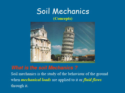
(Concepts)
What is the soil Mechanics ?
Soil mechanics is the study of the behaviour of the ground when mechanical loads are applied to it or fluid flows through it.
Example
General pore Pressure Expression
During Undrained Loading Skemption equation(1948) u=u0+u1=B(1+A(1 -3)) =B3+AB(1 - 3 ) • isotropic stress • uniaxial deviatoric stress
3. Polluted ground clean-up • Anything which rests on the ground or goes through it involves soil mechanics 1. Making a mud pie or a sand castle
2. Leaving footprints in a muddy field or on beach What do we do ? Research, in practice, Make many educated “guesses” based on experience and cleaver investigation and interpretive methods
The pore pressure parameter B = 1 for 100% saturated soil (B 0.95) A depends on the consolidation history of the soil
土力学 (8)

(a) Laminar flow: streamline parallel to each other (b) Turbulent flow: streamline interlace with each other Judgement method : Reynolds number
Outline of Chapter 2
Introduction Capillary phenomena Underground water movement Darcy’s law Determination of permeability
coefficient Seepage force and critical hydraulic
Soil Mechanics-chapter2
Seepage phenomeБайду номын сангаасa
Soil Mechanics-chapter2
Capillary phenomena
In fine-grained soils ,water is capable of rising to a considerable height above the water table and remaining there permanently. This kind of water is called capillary water. The soil layer wetted by capillarity is called capillary water zone and it can be divided into 3 parts. (1) Normal capillary zone ; (2) Capillary network zone; (3) Capillary suspension zone.
Soil Mechanics

Soil MechanicsSoil mechanics is concerned with the use of the laws of mechanics and hydraulics in engineering problems related to soils.Soil is a natural aggregate of mineral grains,with or without organic constituents,formed by the chemical and mechanical weathering of rock.It consists of three phases:solid mineral matter,water,and air or other gas.Soils are extremely variable in composition,and it was this heterogeneity that long discouraged scientific studies of these deposits.Gradually,the investigation of failures of retaining walls,foundations,embankments,pavements,and other structures resulted in a body of knowledge concerning the nature of soils and their behavior sufficient to give rise to soil mechanics as a branch of engineering science.History.Little progress was made in dealing with soil problems on a scientific basis until the latter half of the 18th century,when the French physicist Charles-Augustin de Coulomb published his theory of earth pressure(1773).In 1857 the Scottish engineer Willliam Rankine developed a theory of equilibrium of earth masses and applied it to some elementary problems of foundation engineering.These two classical theories still form the basis of current methods of estimating earth pressure,even though they were based on the misconception that all soils lack cohesion,as does dry sand.Twentieth-century advances have been in the direction of taking cohesion into account understanding the basic physical properties of soils in general and of the plasticity of clay in particular;and systematically studying the shearing characteristics of soils—that is,their performance under conditions of sliding.Both Coulomb’s and Rankine’s theories assumed that the surface of rupture of soil subjectedto a shearing force is a plane.While this is a reasonable approximation for sand,cohesive soils tend to slip along a curved surface.In the early 20th century,Swedish engineers proposed a circular arc as the surface of slip.During the last half century considerable progress has been made in the scientific study of soils and in the application of theory and experimental data to engineering design.A significant advance was made by the German engineer Karl Terzaghi,who in 1925 published a mathematical investigation of the rate of consolidation of clays under applied pressures.His analysis,which was confirmed experimentally, explained the time lag of settlements of fully waterlogged clay deposits.Terzaghi coined the term soil mechanics in 1925 when he published the book Erdbaumechanik(“Earth-Building Mechanics”).Research on subgrade materials,the natural foundation under pavements,was begun about 1920 by the U.S.Bureau of Public Roads.Several simple tests were correlated with the propertiesof natural soils in relation to pavement design.In England,the Road Research Board was set up in 1933.In 1936 the first international conference on soils was held at Harvard University.Today,the civil engineer relies heavily on the numerical results of tests to reinforce experience and correlate new problems with established solutions.Obtaining truly representative sample of soils for such tests,however,is extremely difficult;hence there is a trend toward testing on the site instead of in the laboratory,and many important properties are now evaluatedin this way.Engineering properties of soils.The properties of soils that determine their suitability for engineering use include internal friction,cohesion,compressibility,elasticity,permeability,and capillary.Internal friction is the resistance to sliding offered by the soil mass.Sand and gravel have higher internal friction than clays;in the latter an increase in moisture lowers the internal friction.The tendency of a soil to slide under the weight of a structure may be translated into shear;that is,a movement of a mass of soil in a plane,either horizontal,vertical,or other.Sucha shearing movement involves a danger of building failure.Also resisting the danger of shear is the property of cohesion,which is the mutual attractionof soil particles due to molecular forces and the existence of moisture between them.Cohesive forces are markedly affected by the amount of moisture present.Cohesion is generally very highin clays but almost nonexistent in sands or slits.Cohesion values range from zero for dry sand to 2,000 pounds per square foot for very stiff clays.Compressibility is an important soil characteristic because of the possibility of compacting the soil by rolling,tamping,vibration,or other means,thus increasing its density and load-bearing strength.An elastic soil tends to resume its original condition after compaction.Elastic(expansible)soils are unsuitable as sub-grades for flexible pavements since they compact and expand as a vehicle passes over them,causing failure of the pavement.Permeability is the property of a soil that permits the flow of water through it.Freezing-thawing cycles in winter and wetting-drying cycles in summer alter the packing density of soil grains.Permeability can be reduced by compaction.Capillarity causes water to rise through the soil above the normal horizontal plane of free water.In most soils numerous channels for capillary action exist;in clays,moisture may be raised as much as 30 feet by capillarity.Density can be determined by weight and volume measurements or by special measuring devices.Stability of soils is measured by an instrument called a stabilometer,which specifically measures the horizontal pressure transmitted by a vertical load.Consolidation is the compaction or pressing together of soil that occurs under a specific load condition; this property is also tested.Site Investigation.Soil surveys are conducted to gather data on the nature and extent of the soil expected to be encountered on a project.The amount of effort spent on site investigation depends on the size and importance of the project; it may range from visual inspection to elaborate subsurface exploration by boring and laboratory testing.Collection of representative samples is essential for proper identification and classification of soils.The number of samples taken depends on previously available data, variation in soil types,and the size of the project.Generally,in the natural profile at a location,there is more variation in soil characteristics with depth than with horizontal distance.It is not good practice to collect composite samples for any given horizon (layer),since this does not truly represent any one location and could prove misleading.Even slight variations in soil characteristics in a horizon should be duly noted.Classification of the soilin terms of grain size and the liquid and plastic limits are particularly important steps.An understanding of the eventual use of the data obtained during site investigation is important.Advance information on site conditions is helpful in planning any survey program.Information on topography,geological features(outcrops,road and stream cuts,lake beds,weathered remnants,etc.),paleontological maps,aerial photographs,well logs,and excavations can prove invaluable. Geophysical exploration methods yield useful corroboratory data.Measurement of the electrical resistivity of soils provides an insight intoseveral soil characteristics.Seismic techniques often are used to determine the characteristics of various subsurface strata by measuring the velocity of propagation of explosively generated shock waves through the strata.The propagation velocity varies widely for different types of soils.Shock waves also are utilized to determine the depth of bedrock by measuring the time required for the shock wave to travel to the bedrock and return to the surface as a reflected wave.Dependable subsurface information can only be obtained by excavation.A probe rod pushed into the ground indicates the penetration resistance.Water jets or augers are used to bring subsurface materials to the surface for examination.Colour change is one of the significant elements such an examination can reveal.Various drilling methods are employed to obtain chips from depth.Trenches or pits provide more complete information for shallow depths.Pneumatic or diamond drilling may be required if hard rock is encountered.At least a few of the boreholes should exceed the depth of significant stress that is established for the structure.Avoidance of structural disturbance of the samples is not critical for some tests but is very important for in-place density or shearing strength measurements.Complete and accurate records,such as borehole logs,must be prepared and maintained,and the samples themselves must be retained for future inspection.。
重庆大学土木工程学院土力学第1章

第一章土的物理性质和压实机理主要内容介绍土的形成及物质组成,从定性和定量两个方面描述土体的物质组成\密实程度及工程应用§1 土的物性与分类§1.1 土的形成及颗粒特征§1.2土的结构及工程性质§1.3土的三相组成及物理性质指标§1.4无粘性土的密实特性§1.5粘性土的物理特性§1.6土的工程分类§1.7土的压实机理及工程控制知识要点1.掌握土体的三相组成及三相比例指标之间的换算2.领会无粘性土密实度概念、判别方法及砂土相对密度的计算3.掌握粘性土的塑性、液限、塑性指数和液性指数的概念及其物理状态评价4.掌握无粘性土和粘性土的分类依据和分类方法5.掌握土体的压实原理及压实标准与控制Soil mechanics Chapter 1 (WRH)§ 1.1 土的形成与颗粒特征一、土的形成形成过程形成条件物理力学性质影响土是岩石经过风化后,在不同条件下形成的自然历史的产物搬运、沉积风化岩石地球土地球Soil mechanicsChapter 1 (WRH)生物风化物理风化化学风化矿物成分未变无粘性土原生矿物矿物成分改变粘性土次生矿物风化作用分类有机质岩石和土的粗颗粒受各种气候因素的影响产生胀缩而发生裂缝,或在运动过程中因碰撞和摩擦而破碎。
特点:只改变颗粒的大小和形状,不改变矿物颗粒的成分。
母岩表面和碎散的颗粒受环境因素的作用而改变其矿物的化学成分,形成新的矿物。
经化学风化生成的土为细粒土,具有粘结力。
动植物活动引起的岩石和土体粗颗粒的粒度或成分的变化Soil mechanics Chapter 1 (WRH)残积土无搬运运积土有搬运土质较好残积土强风化弱风化微风化母岩体颗粒表面粗糙多棱角粗细不均无层理母岩表层经风化作用破碎成岩屑或细小颗粒后,未经搬运残留在原地的堆积物风化所形成的土颗粒,受自然力的作用搬运到远近不同的地点所沉积的堆积物二. 搬运与沉积Soil mechanics Chapter 1 (WRH)运积土的特点运积土有搬运风:风积土重力:坡积土流水:洪积土冲积土湖泊沼泽沉积土海相沉积物冰川: 冰积土土粒粗细不同,性质不均匀有分选性,近粗远细浑圆度分选性明显,土层交迭含有机物淤泥,土性差颗粒细,表层松软,土性差土粒粗细变化较大,性质不均匀颗粒均匀,层厚而不具层理Soil mechanics Chapter 1 (WRH)二、土的三相组成气相固相液相++构成土骨架,起决定作用重要影响土体次要作用土体三相组成示意图湿土。
土壤物理学-课后习题

土壤物理学第一章土壤基质以及基质特征1、什么是土壤的基质?基质一词有什么特别的含义?土壤基质特征指的什么?土壤基质:土壤固体部分的物理结构状态称为土壤基质,是一个多分散多孔的体系。
与土壤固体一词相比,土壤基质一词更强调土壤的分散和多孔的特性。
土壤基质的分散性是指土壤的固体物质是由不同比例的、粒径粗细不一、形状和组成各异的颗粒物所组成。
自然土壤一般由分散的粒径不同的土粒和团粒组成。
各分散的土粒和团粒以及团粒内必然存在许多孔隙,大多数土壤基质中的孔隙所占的容积为一半左右,一般用孔隙度来表示。
基质特征通常包括土粒和团粒的粒径分布,土壤比表面积和土壤孔径分布。
有时可包括有机胶体的数量和粘粒矿物的种类。
土壤基质特征是土壤成土过程的产物,是物理和能量在土壤中保持和运动以及植物生长的基础或介质。
不了解土壤基质特征,也就无法了解土壤各项运动过程的真实状况。
2、哪种土壤结构最好?土壤的团粒结构最好,土壤团粒结构中由若干土壤单粒粘结在一起形成为团聚体的一种土壤结构。
因为单粒间形成小孔隙、团聚体间形成大孔隙,所以与单粒结构相比较,其总孔隙度较大。
小孔隙能保持水分,大孔隙则保持通气,团粒结构土壤能保证植物根的良好生长,适于作物栽培。
团粒是由多种微生物分泌的多糖醛酸甙、粘粒矿物以及铁、铅的氢氧化物和腐殖质等胶结而成的。
总之土壤团粒结构是通过干湿交替、温度变化等物理过程,化学分解和合成等化学过程,高等植物根、土壤动物和菌类的活动等生物过程以及人为耕作等农业措施因素而形成的,其中以人类耕作等农业措施对土壤团粒结构的形成影响最大。
良好团粒结构具备的条件:①有一定的结构形态和大小;②有多级孔隙;③有一定的稳性;④有抵抗微生物分解破碎的能力。
团粒结构对土壤肥力的作用:①能协调水分和空气的矛盾;②能协调土壤有机质中养分的消耗和积累的矛盾;③能稳定土壤温度,调节土热状况;④改良耕性和有利于作物根系伸展。
?3、某人做土壤粒径分析实验,得到土样各粒级占干重的百分率如下:根据以上数据,求做土壤粒径分布图,并根据国际、美国、前苏联和中科院南土所所确定的土壤质地划分标准确定供试土样质地。
土木项目工程博士英语必备

⼟⽊项⽬⼯程博⼠英语必备.-⼟⽊⼯程博⼠研究⽣专业英语必备第⼀部分必须掌握,第⼆部分尽量掌握第⼀部分:1 Finite Element Method 有限单元法2 专业英语Specialty English3 ⽔利⼯程Hydraulic Engineering4 ⼟⽊⼯程Civil Engineering5 地下⼯程Underground Engineering6 岩⼟⼯程Geotechnical Engineering7 道路⼯程Road (Highway) Engineering8 桥梁⼯程Bridge Engineering9 隧道⼯程Tunnel Engineering10 ⼯程⼒学Engineering Mechanics11 交通⼯程Traffic Engineering12 港⼝⼯程Port Engineering13 安全性safety17⽊结构timber structure18 砌体结构masonry structure19 混凝⼟结构concrete structure20 钢结构steelstructure21 钢-混凝⼟复合结构steel and concrete composite structure22 素混凝⼟plain concrete 23 钢筋混凝⼟reinforced concrete24 钢筋rebar25 预应⼒混凝⼟pre-stressed concrete26 静定结构statically determinate structure27 超静定结构statically indeterminate structure28 桁架结构truss structure29 空间⽹架结构spatial grid structure30 近海⼯程offshore engineering31 静⼒学statics32运动学kinematics33 动⼒学dynamics34 简⽀梁simply supported beam35 固定⽀座fixed bearing36弹性⼒学elasticity37 塑性⼒学plasticity38 弹塑性⼒学elaso-plasticity39 断裂⼒学fracture Mechanics40 ⼟⼒学soil mechanics41 ⽔⼒学hydraulics42 流体⼒学fluid mechanics43 固体⼒学solid mechanics44 集中⼒concentrated force45 压⼒pressure46 静⽔压⼒hydrostatic pressure .-47 均布压⼒uniform pressure48 体⼒body force49 重⼒gravity50 线荷载line load51 弯矩bending moment52 torque 扭矩53 应⼒stress54 应变stain55 正应⼒normal stress56 剪应⼒shearing stress57 主应⼒principal stress58 变形deformation59 内⼒internal force60 偏移量挠度deflection61 settlement 沉降62 屈曲失稳buckle63 轴⼒axial force64 允许应⼒allowable stress65 疲劳分析fatigue analysis66 梁beam67 壳shell68 板plate69 桥bridge70 桩pile71 主动⼟压⼒active earth pressure72 被动⼟压⼒passive earth pressure 73 承载⼒load-bearing capacity74 ⽔位water Height75 位移displacement76 结构⼒学structural mechanics77 材料⼒学material mechanics78 经纬仪altometer79 ⽔准仪level80 学科discipline81 ⼦学科sub-discipline82 期刊journal ,periodical83⽂献literature84 ISSN International Standard Serial Number 国际标准刊号85 ISBN International Standard Book Number 国际标准书号86 卷volume87 期number 88 专著monograph89 会议论⽂集Proceeding90 学位论⽂thesis, dissertation91 专利patent92 档案档案室archive93 国际学术会议conference94 导师advisor95 学位论⽂答辩defense of thesis96 博⼠研究⽣doctorate student97 研究⽣postgraduate99 SCI Science Citation Index 科学引⽂索引100ISTP Index to Science and Technology Proceedings 科学技术会议论⽂集索引101 题⽬title102 摘要abstract103 全⽂full-text104 参考⽂献reference105 联络单位、所属单位affiliation106 主题词Subject107 关键字keyword108 ASCE American Society of Civil Engineers 美国⼟⽊⼯程师协会109 FHWA Federal Highway Administration 联邦公路总署110 ISO International Standard Organization111 解析⽅法analytical method112 数值⽅法numerical method113 计算computation114 说明书instruction115 规范Specification, Code第⼆部分:岩⼟⼯程专业词汇1.geotechnical engineering岩⼟⼯程2.foundation engineering基础⼯程3.soil, earth⼟ cyclic loading周期荷载unloading卸载reloading再加载viscoelastic foundation粘弹性地基viscous damping粘滞阻尼shear modulus剪切模量5.soil dynamics⼟动⼒学6.stress path应⼒路径7.numerical geotechanics 数值岩⼟⼒学⼆. ⼟的分类 1.residual soil残积⼟ groundwater level地下⽔位 2.groundwater 地下⽔ groundwater table地下⽔位 3.clay minerals粘⼟矿物 4.secondary minerals次⽣矿物/doc/6dd42ba0f4335a8102d276a20029bd64793e6290.html ndslides滑坡 6.bore hole columnar section 钻孔柱状图 7.engineering geologic investigation⼯程地质勘察 8.boulder漂⽯ 9.cobble卵⽯ 10.gravel砂⽯ 11.gravelly sand砾砂 12.coarse sand粗砂 13.medium sand中砂 14.fine sand细砂 15.silty sand粉⼟ 16.clayey soil粘性⼟ 17.clay粘⼟ 18.silty clay粉质粘⼟ 19.silt粉⼟ 20.sandy silt砂质粉⼟ 21.clayey silt粘质粉⼟ 22.saturated soil饱和⼟ 23.unsaturated soil⾮饱和⼟24.fill (soil)填⼟ 25.overconsolidated soil超固结⼟ 26.normally consolidated soil正常固结⼟ 27.underconsolidated soil⽋固结⼟ 28.zonal soil区域性⼟ 29.soft clay软粘⼟ 30.expansive (swelling) soil膨胀⼟ 31.peat泥炭 32.loess黄⼟ 33.frozen soil冻⼟ 24.degree of saturation饱和度 25.dry unit weight⼲重度26.moist unit weight湿重度45.ISSMGE=International Society for Soil Mechanics and Ge otechnical Engineering 国际⼟⼒学与岩⼟⼯程学会四. 渗透性和渗流1.Darcy’s law 达西定律2.piping管涌3.flowing soil流⼟4.sand boiling砂沸5.flow net流⽹6.seepage渗透(流)7.leakage渗流8.seepage pressure渗透压⼒9.permeability渗透性10.seepage force渗透⼒11.hydraulic gradient⽔⼒梯度 12.coefficient of permeability 渗透系数五. 地基应⼒和变形1.soft soil软⼟2.(negative) skin friction of driven pile打⼊桩(负)摩阻⼒3.effective stress有效应⼒4.total stress总应⼒5.field vane shear strength⼗字板抗剪强度6.low activity低活性7.sensitivity灵敏度8.triaxial test三轴试验9.foundation design基础设计 10.recompaction再压缩11.bearing capacity承载⼒ 12.soil mass⼟体13.contact stress (pressure)接触应⼒(压⼒)14.concentrated load集中荷载 15.a semi-infinite elastic solid 半⽆限弹性体 16.homogeneous均质 17.isotropic各向同性18.strip footing条基 19.square spread footing⽅形独⽴基础20.underlying soil (stratum ,strata)下卧层(⼟)21.dead load =sustained load恒载持续荷载 22.live load活载 23.short –term transient load短期瞬时荷载24.long-term transient load长期荷载 25.reduced load折算荷载 26.settlement沉降 27.deformation变形 28.casing套管29.dike=dyke堤(防) 30.clay fraction粘粒粒组 31.physical properties物理性质 32.subgrade路基 33.well-graded soil级配良好⼟ 34.poorly-graded soil级配不良⼟ 35.normal stresses正应⼒ 36.shear stresses剪应⼒ 37.principal plane主平⾯38.major (intermediate, minor) principal stress最⼤(中、最⼩)主应⼒ 39.Mohr-Coulomb failure condition摩尔-库仑破坏条件 40.FEM=finite element method有限元法41.limit equilibrium method极限平衡法42.pore water pressure孔隙⽔压⼒43.preconsolidation pressure先期固结压⼒44.modulus of compressibility压缩模量45.coefficent of compressibility压缩系数/doc/6dd42ba0f4335a8102d276a20029bd64793e6290.html pression index压缩指数 47.swelling index 回弹指数 48.geostatic stress⾃重应⼒ 49.additional stress附加应⼒ 50.total stress总应⼒ 51.final settlement最终沉降 52.slip line滑动线六. 基坑开挖与降⽔ 1 excavation开挖(挖⽅) 2 dewatering (基坑)降⽔ 3 failure of foundation基坑失稳4 bracing of foundation pit基坑围护5 bottom heave=basal heave (基坑)底隆起6 retaining wall挡⼟墙7 pore-pressure distribution孔压分布8 dewatering method降低地下⽔位法9 well point system 井点系统(轻型) 10 deep well point深井点 11 vacuum well point真空井点 12 braced cuts⽀撑围护 13 braced excavation⽀撑开挖 14 braced sheeting⽀撑挡板七. 深基础--deep foundation 1.pile foundation桩基础1)cast –in-place灌注桩 diving casting cast-in-place pile沉管灌注桩 bored pile钻孔桩 special-shaped cast-in-place pile机控异型灌注桩 piles set into rock嵌岩灌注桩 rammed bulb pile夯扩桩2)belled pier foundation钻孔墩基础 drilled-pier foundation 钻孔扩底墩 under-reamed bored pier3)precast concrete pile预制混凝⼟桩4)steel pile钢桩 steel pipe pile钢管桩 steel sheet pile钢板桩5)prestressed concrete pile预应⼒混凝⼟桩 prestressed concrete pipe pile预应⼒混凝⼟管桩 2.caisson foundation沉井(箱)3.diaphragm wall地下连续墙截⽔墙 4.friction pile摩擦桩 5.end-bearing pile端承桩 6.shaft竖井;桩⾝ 7.wave equation analysis波动⽅程分析 8.pile caps承台(桩帽) 9.bearing capacity of single pile 单桩承载⼒/doc/6dd42ba0f4335a8102d276a20029bd64793e6290.html teral pile load test单桩横向载荷试验11.ultimate lateral resistance of single pile单桩横向极限承载⼒ 12.static load test of pile单桩竖向静荷载试验 13.vertical allowable load capacity单桩竖向容许承载⼒ 14.low pile cap低桩承台 15.high-rise pile cap⾼桩承台 16.vertical ultimate uplift resistance of single pile单桩抗拔极限承载⼒ 17.silent piling静⼒压桩 18.uplift pile抗拔桩 19.anti-slide pile抗滑桩20.pile groups群桩 21.efficiency factor of pile groups群桩效率系数(η)22.efficiency of pile groups群桩效应 23.dynamic pile testing 桩基动测技术24.final set最后贯⼊度 25.dynamic load test of pile桩动荷载试验26.pile integrity test桩的完整性试验 27.pile head=butt桩头 28.pile tip=pile point=pile toe桩端(头) 29.pile spacing 桩距30.pile plan桩位布置图 31.arrangement of piles =pile layout 桩的布置32.group action群桩作⽤ 33.end bearing=tip resistance桩端阻 34.skin(side) friction=shaft resistance桩侧阻35.pile cushion桩垫 36.pile driving(by vibration) (振动)打桩 37.pile pulling test拔桩试验 38.pile shoe桩靴 39.pile noise打桩噪⾳ 40.pile rig打桩机九. 固结consolidation1.Terzzaghi’s consolidation theory太沙基固结理论2.Barraon’s consolidation theory巴隆固结理论3.Biot’s consolidation theory⽐奥固结理论4.over consolidation ration (OCR)超固结⽐5.overconsolidation soil超固结⼟6.excess pore water pressure超孔压⼒7.multi-dimensional consolidation多维固结8.one-dimensional consolidation⼀维固结9.primary consolidation主固结10.secondary consolidation次固结11.degree of consolidation固结度 12.consolidation test固结试验 13.consolidation curve固结曲线 14.time factor Tv时间因⼦15.coefficient of consolidation固结系数16.preconsolidation pressure前期固结压⼒17.principle of effective stress有效应⼒原理18.consolidation under K0 condition K0固结⼗. 抗剪强度shear strength 1.undrained shear strength不排⽔抗剪强度2.residual strength残余强度3.long-term strength长期强度4.peak strength峰值强度5.shear strain rate剪切应变速率6.dilatation剪胀7.effective stress approach of shear strength 剪胀抗剪强度有效应⼒法 8.total stress approach of shear strength抗剪强度总应⼒法 9.Mohr-Coulomb theory莫尔-库仑理论 10.angle of internal friction内摩擦⾓ 11.cohesion粘聚⼒ 12.failure criterion破坏准则 13.vane strength⼗字板抗剪强度14.unconfined compression⽆侧限抗压强度15.effective stress failure envelop有效应⼒破坏包线16.effective stress strength parameter有效应⼒强度参数⼗⼀. 本构模型--constitutive model1.elastic model弹性模型2.nonlinear elastic model⾮线性弹性模型3.elastoplastic model弹塑性模型4.viscoelastic model粘弹性模型5.boundary surface model边界⾯模型6.Duncan-Chang model邓肯-张模型7.rigid plastic model 刚塑性模型8.cap model盖帽模型9.work softening加⼯软化 10.work hardening加⼯硬化 11.Cambridge model剑桥模型 12.ideal elastoplastic model理想弹塑性模型 13.Mohr-Coulomb yield criterion莫尔-库仑屈服准则14.yield surface屈服⾯15.elastic half-space foundation model弹性半空间地基模型 16.elastic modulus弹性模量 17.Winkler foundation model ⽂克尔地基模型⼗⼆. 地基承载⼒--bearing capacity of foundation soil 1.punching shear failure冲剪破坏 2.general shear failure整体剪切破化3.local shear failure局部剪切破坏 4.state of limit equilibrium极限平衡状态5.critical edge pressure临塑荷载6.stability of foundation soil地基稳定性7.ultimate bearing capacity of foundation soil地基极限承载⼒ 8.allowable bearing capacity of foundation soil地基容许承载⼒⼗三. ⼟压⼒--earth pressure1.active earth pressure主动⼟压⼒2.passive earth pressure被动⼟压⼒3.earth pressure at rest静⽌⼟压⼒4.Coulomb’s earth pressure theory库仑⼟压⼒理论5.Rankine’s earth pressure theory朗⾦⼟压⼒理论⼗四. ⼟坡稳定分析--slope stability analysis1.angle of repose休⽌⾓2.Bishop method毕肖普法3.safety factor of slope边坡稳定安全系数4.Fellenius method of slices费纽伦斯条分法5.Swedish circle method瑞典圆弧滑动法6.slices method条分法⼗五. 挡⼟墙--retaining wall1.stability of retaining wall挡⼟墙稳定性2.foundation wall基础墙3.counter retaining wall扶壁式挡⼟墙4.cantilever retaining wall悬臂式挡⼟墙5.cantilever sheet pile wall悬臂式板桩墙6.gravity retaining wall重⼒式挡⼟墙7.anchored plate retaining wall锚定板挡⼟墙8.anchored sheet pile wall锚定板板桩墙⼗六. 板桩结构物--sheet pile structure1.steel sheet pile钢板桩2.reinforced concrete sheet pile钢筋混凝⼟板桩3.steel piles钢桩4.wooden sheet pile⽊板桩5.timber piles⽊桩⼗七. 浅基础--shallow foundation 1.box foundation箱型基础 2.mat(raft) foundation⽚筏基础 3.strip foundation条形基础4.spread footing扩展基础 /doc/6dd42ba0f4335a8102d276a20029bd64793e6290.html pensated foundation补偿性基础 6.bearing stratum持⼒层 7.rigid foundation刚性基础 8.flexible foundation柔性基础9.embedded depth of foundation基础埋置深度/doc/6dd42ba0f4335a8102d276a20029bd64793e6290.html foundation pressure基底附加应⼒11.structure-foundation-soil interaction analysis上部结构-基础-地基共同作⽤分析⼗⼋. ⼟的动⼒性质--dynamic properties of soils1.dynamic strength of soils动强度2.wave velocity method 波速法3.material damping材料阻尼4.geometric damping ⼏何阻尼5.damping ratio阻尼⽐6.initial liquefaction初始液化7.natural period of soil site地基固有周期8.dynamic shear modulus of soils动剪切模量 9.dynamic ma ⼆⼗. 地基基础抗震1.earthquake engineering地震⼯程2.soil dynamics⼟动⼒学3.duration of earthquake地震持续时间4.earthquake response spectrum地震反应谱5.earthquake intensity地震烈度6.earthquake magnitude震级7.seismic predominant period地震卓越周期 8.maximum acceleration of earthquake地震最⼤加速度⼆⼗⼀. 室内⼟⼯实验1.high pressure consolidation test⾼压固结试验 2.consolidation under K0 condition K0固结试验 3.falling head permeability变⽔头试验4.constant head permeability常⽔头渗透试验5.unconsolidated-undrained triaxial test不固结不排⽔试验(UU)6.consolidated undrained triaxial test固结不排⽔试验(CU)7.consolidated drained triaxial test固结排⽔试验(CD)/doc/6dd42ba0f4335a8102d276a20029bd64793e6290.html paction test击实试验9.consolidated quick direct shear test固结快剪试验10.quick direct shear test快剪试验11.consolidated drained direct shear test慢剪试验12.sieve analysis筛分析 13.geotechnical model test⼟⼯模型试验 14.centrifugalmodel test离⼼模型试验15.direct shear apparatus直剪仪 16.direct shear test直剪试验 17.direct simple shear test直接单剪试验18.dynamic triaxial test三轴试验 19.dynamic simple shear动单剪 20.free(resonance)vibration column test⾃(共)振柱试验⼆⼗⼆. 原位测试1.standard penetration test (SPT)标准贯⼊试验2.surface wave test (SWT)表⾯波试验3.dynamic penetration test(DPT)动⼒触探试验4.static cone penetration (SPT) 静⼒触探试验5.plate loading test静⼒荷载试验/doc/6dd42ba0f4335a8102d276a20029bd64793e6290.html teral load test of pile 单桩横向载荷试验7.static load test of pile 单桩竖向荷载试验8.cross-hole test 跨孔试验9.screw plate test螺旋板载荷试验10.pressuremeter test旁压试验11.light sounding轻便触探试验12.deep settlement measurement深层沉降观测13.vane shear test⼗字板剪切试验14.field permeability test现场渗透试验15.in-situ pore water pressure measurement 原位孔隙⽔压量测16.in-situ soil test原位试验。
现代土壤力学
第一章 大地工程-歷史的回顧 第7頁
1.6 現代土壤力學(1910-1927)
在此一時期,經由黏土相關研究所發表之著作建 立了黏土基本行為與參數,其中最重要之著作敘 述於下。
1911 年,瑞典化學與土壤科學家Albert Mauritz Atterberg(1846-1916),以定義液性、塑性與縮性限 度來解釋黏土的稠性。 法國工程師Jean Frontard(1884-1962)在一等值垂直 壓力下為黏土試體進行不排水雙向剪力試驗,來決定 其剪力強度參數(參見Frontard, 1914)。
在1700 至1927 年間之大地工程可分成四個階段 (Skempton,1985):
1. 2. 3. 4. 前古典時期(西元1700 至1776 年)。 古典土壤力學── 第1 期(西元1776 至1856 年)。 古典土壤力學── 第2 期(西元1856 至1910 年)。 現代土壤力學(西元1910 至1927 年)。
第一章 大地工程-歷史的回顧 第4-5頁
1.3 前古典時期(1700-1776)
此一時期的研究重點,是關於各種土壤之天然邊 坡和單位重,以及半經驗法則之土壓力理論。 1717 年法國皇家工程師Henri Gautier(16601737),根據使用土壤堆積而自然形成有尖頂斜 坡的研究來推導擋土牆設計程序。當時所謂自然 形成斜坡之斜率(natural slope),就是我們現在 所說的安息角(angle of repose)。根據此一研究, 乾淨之乾砂土(dry sand)與一般土壤(ordinary earth)的安息角分別為31° 與45°。
第一章 大地工程-歷史的回顧 第5頁
1.3 前古典時期(1700-1776)
第一章 大地工程-歷史的回顧 第5頁
河海大学土力学英文教案Chapter 2 Permeability of Soil
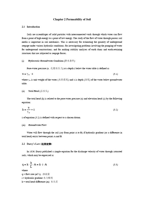
Chapter 2 Permeability of Soil2.1 IntroductionSoils are assemblages of solid particles with interconnected voids through which water can flow from a point of high energy to a point of low energy. The study of the flow of water through porous soil media is important in soil mechanics. This is necessary for estimating the quantity of underground seepage under various hydraulic conditions; for investigating problems involving the pumping of water for underground constructions; and for making stability analyses of earth dams and earth-retaining structures that are subjected to seepage forces. (i) Hydrostatic Groundwater Condition (静水条件)Pore-water pressure (u, 孔隙水压力) at a depth z below the water table is defined as z u w ⋅γ=(3.1)where γw is unit weight of the water (水的重度) and z is depth (深度) of the water below groundwatertable. (ii) Total Head (总水头)The total head (h) is related to the pore-water pressure (u) and elevation head (z) by the followingequation:z uh w+γ=(3.2)z of equation (3.2) is defined with respect to a chosen datum.(iii) Groundwater FlowWater will flow through the soil (say from point A to B) if hydraulic gradient (or a difference in total head) exists between points A and B.2.2 Darcy ’s Law (达西定律)In 1856, Darcy published a simple equation for the discharge velocity of water through saturated soils, which may be expressed asA i k A Lhk q ⋅⋅=⋅⋅= (3.3)whereq = flow rate (m 3/s), 渗流量 i = hydraulic gradient 水力梯度 h = total head difference (m) 水头差L = length of flow (m) 渗径长度k = coefficient of permeability (m/s) 渗透系数 A = cross-sectional area of the specimen (m 2) 横截面积Equation (3.3) implies that the flow rate (q) bears a linear relationship to the hydraulic gradient (i). However, a non-linear relationship between q and i is found for clay [叁考: 土力学 p.69 图 3-3]. For practical reason, the following relationship between q and i is assumed for clay:()A i i k q b ⋅-⋅=(3.3a)where i b is starting hydraulic gradient (起始水力梯度). For gravelly soil (砾土), linear relationship between q and i appears at small hydraulic gradient only. As hydraulic gradient increases beyond a critical value, the relationship becomes non-linear as the flow becomes turbulent (紊流) [叁考: 土力学 p.69 图 3-3].Darcy ’s law is valid for laminar flow (层流) condition where Reynolds numbers is smaller than or equal to 1. Reynolds numbers (雷诺数) is defined as follows:1dv Re ≤η⋅⋅ρ=(3.4)where ρ is density of water (水的密度), v is velocity of water (流速), η is viscosity of water (水的粘滞系数) and d is average diameter of soil grains (土粒子平均粒径). As ρ = 1 g/cm 3, v = 0.25 cm/s, η = 0.0131 g/s ⋅cm at temperature of 10︒C, d is calculated by equation (3.4)m m 52.0v0.1d ≤⋅ρη⋅≤Thus Darcy ’s law can be applied to soils which are finer than coarse sand.2.3 Determination of Coefficient of Permeability (渗透系数的测定)2.3.1Constant head test (常水头测试)A typical arrangement of the constant head permeability test is shown in Fig.2.1. In the setup, the total water head is always maintained constant during the period of the test. The constant head test is suitable for coarse-grained soils. The coefficient of permeability is calculated by the following equation:t h A LV Lh t A V i v k ⋅∆⋅⋅=∆⋅== (3.5)where V is volume of water collected, L is length of the specimen, A is cross-sectional area of the specimen, ∆h is total head difference and t is duration of the test.2.3.2 Falling Head Test (变水头测试)A typical arrangement of the falling head permeability test is shown in Fig.2.2. It is suitable for fine-grained soils. The rate of flow of water through the specimen at any time t is given bydtdhA A L h k dt dV 21⋅-=⋅⋅= (3.6a)where V is volume of water collected, L is length of the specimen, A 1 is cross-sectional area of the specimen, A 2 is cross-sectional area of the standpipe and h is total head difference. Re-arranging equation (3.6a) into⎪⎭⎫⎝⎛-⋅⋅=h dh k A L A dt 12(3.6b)Integrating equation (3.6b)⎪⎭⎫⎝⎛-⋅⋅⋅=⎰⎰h dh k A L A dt 21h h 12T⎪⎪⎭⎫ ⎝⎛⋅⋅⋅=2112h h ln k A L A T ⎪⎪⎭⎫ ⎝⎛⋅⋅⋅=2112h h ln T A L A k(3.6c)The values of k for different types of soil are typically within the ranges shown in Table 2.1.2.4 Seepage and Flow Nets (渗流和流网)2.4.1 Laplace ’s equationLaplace differential equation of continuity is used to describe the two-dimensional steady flow condition for a given point in the soil mass. Let us consider a soil element as shown in Fig. 2.3. The element has dimension of dx and dz in x and z direction, respectively. Water flows through the element due to a hydraulic head difference between upstream and downstream side. Let v x and v z be the discharge velocity in the x and z direction, respectively. The rates of flow of water into the element in the x and z direction are1dz v q x )in (x ⋅⋅= (3.7a) 1dx v q z )in (z ⋅⋅=(3.7b)The rates of flow of water out of the element in the x and z direction are1dz dx x v v q x x )out (x ⋅⋅⎪⎭⎫⎝⎛∂∂+=(3.7c)1dx dz z v v q z z )out (z ⋅⋅⎪⎭⎫⎝⎛∂∂+=(3.7d)Assuming water is incompressible and no volume change in the soil mass occurs, the total rate of inflow should be equal to the total rate of outflow1dx v 1dz v 1dx dz z v v 1dz dx x v v z x z z x x ⋅⋅+⋅⋅=⋅⋅⎪⎭⎫⎝⎛∂∂++⋅⋅⎪⎭⎫ ⎝⎛∂∂+0zv x v z x =∂∂+∂∂(3.7e)Using Darcy ’s law, v x and v z can be expressed asx hk i k v x x x x ∂∂⋅=⋅= (3.7f) z h k i k v z z z z ∂∂⋅=⋅=(3.7g)Substituting equations (3.7f) and (3.7g) into equation (3.7e)0zhk x h k 22z 22x =∂∂⋅+∂∂⋅(3.7h)If the soil is isotropic k x = k z , equation (3.7h) becomes0z h x h 2222=∂∂+∂∂ (3.7i)2.4.2 Flow NetsThe continuity equation [equation(3.7i)] in isotropic medium represents two orthogonal families of curves – that is, the flow lines (流线) and equipotential lines (等势线).A flow line is a line along which a water particle will travel from upstream to the downstream side in the permeable soil medium. An equipotential line is a line along which the total head (总水头) at all points is the same. If piezometers (测压计) are placed at different points along an equipotential line, the height of water will rise to the same elevation in all of them. A combination of a number of flow lines and equipotential lines is called a flow net.To complete the graphical construction of a flow net, the flow and equipotential lines are drawn in such a way that (i) the equipotential lines intersect the flow lines at right angle, (ii) the flow elements are approximate squares, (iii) the upstream and downstream surfaces of the permeable layer are equipotential lines and (iv) the boundary of the impervous layer is a flow line.Based on the flow net, the total flow rate (q) can be estimated bydfN N H k q ⋅⋅= (3.8)where H is the total head difference between the upstream and downstream sides, N f is the number of flow channels and N d is the number of equipotential drops.In addition, the pore-water pressure (u) at a given point A determined from the flow net is⎪⎪⎭⎫ ⎝⎛⋅-=d dt Nn H H h (3.9a)()w e t h h u γ⋅-=(3.9b)where H is total head difference, N d is total number of equipotential drops, n d is number of equipotential drops at point A, h t is total head at point A and h e is elevation head at point A.2.5 Effective stress (有效应力)2.5.1 Effective stress principleEffective stress (σ’) is defined asAN 's∑=σ (3.10a)where ∑N s is the sum of inter-contact forces and A is the cross-sectional area of the soil mass under consideration.Total stress (σ) is defined as()u A A N A s s ⋅-+=⋅σ∑()u AA A AN s s⋅-+=σ∑(3.10b)where A s is cross-sectional area of the soil mass occupied by solid-to-solid contacts. As the ratio A s /A is small and can be neglected for pressure ranges encountered in practical problems. Thus, equation (3.10b) becomesu '+σ=σ(3.11)2.5.2 Pore-water pressure and effective stress under hydrostatic conditionThe total stress at depth z isz sat ⋅γ=σ(3.12a)The pore-water pressure at depth z isz u w ⋅γ=(3.12b)The effective stress at depth z is()z 'z u 'w sat ⋅γ=⋅γ-γ=-σ=σ(3.12c)where γsat is saturated unit weight of soil, γw is unit weight of water and γ’ is submerged unit weight ofsoil.2.5.3 Pore-water pressure and effective stress under seepage(i) Downward seepageThe pore-water pressure at depth z is reduced because of the downward flow of waterh z u w w ⋅γ-⋅γ=(3.13a)where h is the hydraulic head difference between ground surface and depth z. The effective stress at depth z becomesh z 'u 'w ⋅γ+⋅γ=-σ=σ(3.13b)(ii) Upward seepageThe pore-water pressure at depth z is increased because of the upward flow of waterh z u w w ⋅γ+⋅γ=(3.14a)where h is the hydraulic head difference between ground surface and depth z. The effective stress at depth z becomesh z 'u 'w ⋅γ-⋅γ=-σ=σ(3.14b)2.5.4 Critical hydraulic gradient (临界水力梯度)At boiling or quick condition under a critical hydraulic gradient (i c ), the weight of the soil will be balanced by the upward seepage force such that the effective stress becomes zero. From equation (3.14b)0h z 'c w =⋅γ-⋅γ()()()n 11G e11G 'z h i s s w c c -⋅-=+-=γγ==(3.15)where e is void ratio and n is porosity.Table 2.1 Typical values of coefficients of permeability (k)Key wordsClay粘土Constant head test 常水头测试Cross-sectional area 横截面积Darcy’s Law 达西定律Density 密度Diameter of soil grains 土粒子粒径Discharge velocity 渗透速度Effective Stress有效应力Equipotential line 等势线Falling head test 变水头测试Flow line 流线Flow net 流网Flow rate 渗流量Gravel 砾石Hydraulic Head 水头Hydraulic head difference 水头差Hydraulic gradient 水力梯度Breaking hydraulic gradient起始水力梯度Critical hydraulic gradient 临界水力梯度Hydrostatic condition静水条件Laminar flow 层流Laplace Equation 拉普拉斯方程Mixture混合物Permeability 渗透性Coefficient of permeability 渗透系数Pore-water pressure孔隙水压力Porosity 孔隙率Reynolds numbers 雷诺数Sand 砂土Seepage 渗流Seepage Force渗流力Silt 粉土Total Stress总应力Turbulent flow 紊流Viscosity 粘滞系数V oid ratio 孔隙比Fig. 2.1 Setup of constant head permeability test Fig. 2.2 Setup of falling head permeability test Fig. 2.3 Seepage through a soil elementChapter 3 Stresses in soil (土体应力)3.1 IntroductionSoil mass can bear loadings from structures as well as its self-weight. Stresses are produced due to these loadings. The stresses are used to evaluate the deformation of the structures founded on the soil mass and the stability of the soil mass. This chapter presents the methods to determine the self weight and additional stresses acted on a soil mass.3.2 In-situ stresses (原位应力)3.2.1 Effective vertical stress (竖向应力)The effective vertical stress (σ’z ) is calculated from the unit weight of the soil (土的重度),γ.(i) No ground water table (地下水位) exists [叁考: 土力学 p.39 图 2-1]z 'z ⋅γ=σ(3.1)where γ (kN/m 3) is unit weight of the soil and z (m) is depth of the soil.(ii) Ground water table locates at the ground surface()z 'z 'w z ⋅γ=⋅γ-γ=σ(3.2)where γ’ (kN/m 3) is submerged unit weight of the soil (土的浮重度) and γw (9.81 kN/m 3) is unit weightof water (水的浮重度).(iii) If the ground consists of n different layers of stratum (土层)i n1i i z z '⋅γ=σ∑=(3.3)where γi and z i are unit weight and depth of the soil of the i th stratum, respectively.3.2.2 Effective horizontal stress (侧向应力)The effective horizontal stress (σ’h ) is much more difficult to be evaluated. Normally, the horizontal stress is expressed as a function vertical stress by the following expression:v o h 'K 'σ⋅=σ(3.4)where K o is coefficient of earth pressure at rest (静止侧压力系数). Typical values of K o are listed inTable 3.1.3.3 Contact pressures at the bottom of the foundation (基底压力)3.3.1 Flexible and rigid foundationsThe pressure distribution beneath a foundation depends on the type of load, the flexural rigidity of the foundation and the type of material on which it is resting.A flexible foundation (柔性基础) has zero stiffness but a rigid foundation (刚性基础) has infinite stiffness. A uniformly loaded flexible foundations (e.g. oil tank and earth dam) resting on an elastic material such as saturated clay will take a sagging profile and the contact pressure is also uniformly distributed [叁考: 土力学 p.41 图 2-4].A rigid foundation (e.g. concrete dam, box foundation) resting on saturated clay will undergo uniform settlement and the contact pressure distribution looks like a saddle, i.e. large at the edge but small in the middle [叁考: 土力学 p.42 图 2-5].If the size of the foundation is not too large and the applied load is small, linear distribution of the contact pressure can be used.3.3.2 Pressure distribution at the bottom of the rigid foundation(i) Vertical load at the center of the foundation (中心竖向荷载)BL F p v⋅=(3.5)where F v is the sum of the applied vertical load (竖向荷载) and the weight of the foundation and backfill (基础和回填土的总重), L is the length of the foundation and B is breadth of the foundation.(ii) Eccentric and vertical load (偏心竖向荷载)⎪⎭⎫⎝⎛±⋅=L e 61B L F }p p v min max (3.6)where e is the eccentricity of the total vertical load.For e < L/6, a trapezoidal pressure distribution, For e = L/6, a triangular pressure distribution,For e > L/6, p min < 0, part of the foundation is separated from the soil and the stress redistributes to a triangular pressure distribution [叁考: 土力学 p.43 图 2-7e] with p max equals to()e L 5.0B 3F 2p vmax -⋅⋅=(3.7)(iii) Net pressure at the bottom of the foundation (基底净压力)Before the construction of a foundation, the soil exhibits an overburden pressure due to its self weight. During construction, soil is excavated to the level of foundation. The final (or net) pressure exerted on the foundation is the applied pressure minus the weight of the excavated soil.o net z p p ⋅γ-=(3.8)where z o is depth of foundation.3.4 Stress increase due to surface load (地基中的附加应力)3.4.1 Stresses due to a vertical point load (竖向集中力作用下附加应力)Boussinesq (1883) solved the problem of stresses produced at any point in a homogeneous (均质), elastic (弹性) and isotropic (各向同性) medium as the result of a point load applied on the surface of a semi-infinite half space (半无限空间体). Boussinesq ’s solution for stresses at a point M [叁考: 土力学 p.47 图 2-10] due to the point load F is()()()⎭⎬⎫⎩⎨⎧⎥⎦⎤⎢⎣⎡-⋅+⋅+-+⋅μ-+⋅π=δσ35252x R z R z R x z R 2z R R 1321R z x 2F 3(3.9a)()()()⎭⎬⎫⎩⎨⎧⎥⎦⎤⎢⎣⎡-+⋅+-+⋅μ-+⋅π=δσ35252y R z R z R y z R 2z R R 1321R z y 2F 3 (3.9b)5332z R z 2F 3cos R2F 3π=θ⋅π=δσ(3.9c)()()⎥⎦⎤⎢⎣⎡⋅++μ--⋅⋅π=δτ=δτ325y x xy R y x z R z R 2321R z y x 2F 3 (3.9d)52zxxz R z x 2F 3⋅π=δτ=δτ(3.9e)52zyy z R z y 2F 3⋅π=δτ=δτ (3.9f)22y x r +=(3.9g) 22222z r z y x R +=++=(3.9h)where μ is Poisson ’s ratio. Equation (3.9c) can be re-arranged as follows:225225253z z F K z r 11z 2F 3R z z 2F 3R z 2F 3⋅=⎥⎥⎦⎤⎢⎢⎣⎡⎪⎭⎫ ⎝⎛+⋅π=⎪⎭⎫⎝⎛⋅π=π=δσ (3.9i)where252z r 123K ⎥⎥⎦⎤⎢⎢⎣⎡⎪⎭⎫ ⎝⎛+⋅π=(3.9j)K is a function of r/z.By using the principle of superposition (叠加原理), the vertical stress produced at point M due to several point loads F i ( i = 1,2,…n) [叁考: 土力学 p.47 图 2-12] can be deduced from equation (3.9j) and presented as follows:∑∑==⋅=⋅=δσn1i i i2n1i 2i i z F Kz 1z F K(3.9k)3.4.2 Stress increase in 3-dimensional problems (空间条件下的附加应力)(i) Vertical stress beneath the corner of a vertical and uniformly loaded (竖直均布荷载) rectangularfoundationLet the net pressure on the rectangular area be equal to p [叁考: 土力学 p.48 图 2-13]. The total load on the elementary area is pdxdy. The vertical stress (d σz ) at point M due to the load on this elementary area can be obtained from equation (3.9c)dy dx p R 2z 3d 53z ⋅⋅⋅π=σ(3.10a)The increase of stress at M due to the entire rectangular loaded area can be found by integratingequation (3.10a)()⎥⎦⎤⎢⎣⎡⎪⎭⎫ ⎝⎛+⎪⎭⎫ ⎝⎛+++++⋅π=++⋅π⋅⋅⋅=⋅π⋅⋅⋅=δσ-⎰⎰⎰⎰n m tan n 11n m 1n m 1nm 2p z y x 2dydx p z 3R 2dy dx p z 3122222B 0L052223B 0L 053z (3.10b)where m = L/B and n = z/B, L is length of the rectangle, B is breadth of the rectangle, z is depth of point A from the bottom of the foundation. Equation (3.10b) can be re-written as follows:p K s z ⋅=σ(3.10c)K s is a function of m and n or L. B and z. Values of K s can be obtained from 土力学 p.52表2-2.(ii) Vertical stress beneath the center of a vertical and uniformly loaded circular foundationLet the net pressure on the circular foundation of radius r o be equal to p [叁考: 土力学 p.52 图 2-18]. The total load on the elementary area is prdrd θ. The vertical stress (d σz ) at point A belowthe center due to the load on this elementary area can be obtained from equation (3.9c) The increase of stress at A due to the entire circular area can be found by integrating d σz()p K r /z 1111p z r 2prdrd z 3d r 2320220r 0522320r 0zz 00⋅=⎥⎥⎥⎥⎥⎥⎦⎤⎢⎢⎢⎢⎢⎢⎣⎡⎪⎪⎭⎫ ⎝⎛+-=+πθ=σ=σ⎰⎰⎰⎰ππ (3.11)K r is a function of z/r 0 and values of K r are summarized in 土力学 p.55表2-5.3.4.3 Stress increase in 2-dimensional problems (平面问题条件下的附加应力)(i) Stresses due to a line load (线荷载)The figure [叁考: 土力学 p.56 图 2-19] shows a line load of infinite length (y direction) having a pressure p/unit length on the surface of a semi-infinite soil mass. The total load on the elementary length is pdy. The vertical stress (d σz ), horizontal stress (d σx ) and shear stress (τxz ) at point A due to the load on this elementary length can be obtained from equations (3.9c), (3.9a) and (3.9e), respectively. The increase of stresses at M due to the entire line load can be found by integrating d σz , d σx and τxz ,β⋅π=⋅π⋅=⋅π⋅⋅=σ⎰+∞∞-3141353z cos R p 2R z p 2R2dy p z 3 (3.12a)β⋅β⋅π=σ21x sin cos R p2(3.12b)β⋅β⋅π=⋅π⋅⋅=τ=τsin cos R p2R z x p 221412zx xz (3.12c)where221z x R += (3.12d) zx tan =β(3.12e)This is a plane stress problem and from theory of elasticity()z x y σ+σ⋅μ=σ(3.12f)(ii) Vertical stress beneath a vertical and uniformly loaded strip foundation (条形基础竖直均布荷载)Equation (3.12a) derived for the vertical stress increases as the result of a line load can be used to determine the stress increases at a point due to a strip load of width B [叁考: 土力学 p.56 图 2-20]. Let the pressure acting on the foundation be p n and consider an elementary strip of of width d ζ. The load per unit length of this strip is p n d ζ. This elementary strip can be treated as a line load. The vertical stress increase (d σz ) is calculated from equation (3.12a) by replacing p by p n d ζ. and xby (x - ζ). The increase of stresses at A due to the entire strip load can be found by integrating d σz ,()[]p K z x d z p 2s z 2223Bz ⋅=+ζ-ζ⋅⋅π=σ⎰(3.13a)where()()⎥⎦⎤⎢⎣⎡-+-⋅-+-+⎪⎭⎫ ⎝⎛--⎪⎭⎫ ⎝⎛⋅π=--222211sz1m n 1m n m n n m n 1m tan n m tan 1K(3.13b)where m = x/B and n = z/B and values of K z s are tabulated in 土力学 p.59表2-6.Table 3.1 Typical values of K oKey wordsClay 粘土Normally consolidated clay 正常固结粘土Overconsolidated clay 超固结粘土Coefficient of earth pressure at rest (K o) 静止侧压力系数Earth dam 土坝Eccentric 偏心Elastic 弹性Fill 填土Backfill 回填土Well-compacted fill 压实填土Foundation 基础Bottom of foundation 基底Flexible foundation 柔性基础Rigid foundation 刚性基础Strip foundation 条形基础Ground water table 地下水位Homogeneous 均质In-situ stresses 原位应力Isotropic 各向同性Load 荷载Horizontal load 水平荷载Inclined load 倾斜荷载Line load 线荷载Triangular load 三角形分布荷载Uniform load 均布荷载Vertical load 竖向荷载Vertical point load 竖向集中力Moment 力矩Pressure 压力Net pressure 净压力Principle of superposition 叠加原理Right-angled trapezoidal load 直角梯形分布荷载Sand 砂土Loose sand 松砂Dense sand 密砂Semi-infinite half space 半无限空间体Stratum 土层Stress 应力Horizontal stress 侧向应力Stress increase 附加应力Vertical stress 竖向应力Two-dimensional problem 平面问题Unit weight of soil 土的重度Submerged unit weight of soil 土的浮重度Chapter 4 Compressibility and Consolidation of Soil [土的压缩与固结]4.1 IntroductionThe process of consolidation [固结] is often confused with the process of compaction [压实]. Compaction increases the density of an unsaturated soil by reducing the volume of air in the voids (see Fig.4.1). However, consolidation is a time-related process of increasing the density of a saturated soil by draining some of the water out of the voids (see Fig.4.1).Consolidation is generally related to fine-grained soils [幼粒土] such as silts and clays. Coarse-grained soils [粗粒土], such as sands and gravels, also undergo consolidation but at a much faster rate due to their high permeability. Saturated clays consolidate at a much slower rate due to their low permeability.Consolidation theory is required for the prediction of both the magnitude and the rate of consolidation settlements [沉降量与沉降速度] to ensure the serviceability of structures founded on a compressible soil layer.4.2 A simple one-dimensional consolidation model [单向固结模型]Since water can flow out of a saturated soil in any direction, the process of consolidation is essentially three-dimensional [三维]. However, in most field situations, water will not be able to flow out of the soil by flowing horizontally because of the vast expanse of the soil in horizontal direction. Therefore, the direction of flow of water is primarily vertical [竖向] or one-dimensional. As a result, the soil layer undergoes one-dimensional (1-D) consolidation settlement [单向固结沉降] in the vertical direction.Fig.4.2 shows a simple model for 1-D consolidation. The spring [弹簧] is analogous to the soil skeleton [土骨架]. The stiffer the spring, the less it will compress. Therefore, a stiff soil will undergo less compression than a soft soil. The stiffness of a soil [土的硬度] influences the magnitude of its consolidation settlement. The valve [阀门] opening size is analogous to the permeability of the soil [土的渗透性]. The smaller the opening, the longer it will take for the water to flow out and dissipate its pressure. Therefore, consolidation of a fine-grained soil takes longer to complete than that of a coarse-grained soil. Permeability of a soil influences the rate of its consolidation.4.3 One-dimensional consolidation test [单向固结试验]The one-dimensional (1-D) consolidation test is performed in an oedometer [固结仪]. An oedometer is shown in Fig.4.3. The soil specimen [土样本] is in a form of a disc (normally 20 mm in height and 80 mm in diameter), which is confined in a steel ring and immersed in a water bath. A vertical load [竖向荷载] is applied to compress the specimen and water is permitted to drain away through porous stones [透水石] placed at the top and bottom of the specimen.4.3.1 Time-related consolidationFor each vertical load increment [竖向荷载增量], the vertical settlement [竖向沉降] of the soil specimen is recorded using a dial gauge [百分表]. Fig.4.4 shows the time relationships of verticalsettlement, vertical total stress, excess pore-water pressure [超孔隙水压力] and vertical effective stress. Initially, 100 % of the vertical load is taken by pore water because, due to low permeability of the soil specimen, the pore water is unable to flow out of the voids quickly. Therefore, there is very little settlement of the soil specimen immediately after placing the vertical load. The settlement of soil is possible only when there is an increase in effective stress, which in turn requires that the void ratio of the soil be reduced by the expulsion of pore water. After a few seconds, the pore water begins to flow out of the voids. This results in a decrease in excessive pore-water pressure and void ratio of the soil specimen and an increase in effective stress. Finally, all excess pore-water pressure dissipates and the vertical effective stress equals to the vertical total stress.4.3.2 Compression Curve [压缩曲线]Several increments of vertical stress are applied in an oedometer test. For each increment, the final settlement of the soil specimen is recorded. The end points from number of loading and unloading increments [荷载与卸载增量] of an oedometer test may be plotted as a conventional stress-strain curve [应力-应变曲线] as shown in Fig.4.5. The increment of vertical strain [竖向应变增量] (∆εv ) for each loading increment is given byv H h∆=ε∆ (4.1)where ∆h is the final settlement for the loading increment (i.e. the change in specimen height) and H 0 is the initial specimen height [样本初始高度] before loading increment is applied.(i) e : σ’v curveAs the soil specimen is not allowed to deform in horizontal direction, there is only change in void ratio. Thus, ∆εv can be expressed in terms of the void ratio [孔隙比] (e) by0v e 1eH h +∆=∆=ε∆ (4.2)where ∆e is the change in void ratio due to the loading increment and e 0 is the initial void ratio of the specimen [初始孔隙比] before loading increment is applied. The test results are plotted in terms of vertical effective stress (σ’v ) and void ratio (e) and shown in Fig.4.6.The coefficient of volume compressibility [体积压缩系数] (m v ) is defined as the ratio of change in volumetric strain (∆εvol ) over change in vertical effective stress (∆σ’v ) and shown as follows:v o v vol v 'ee 11'm σ∆∆⋅+-=σ∆ε∆= (4.3) The unit for m v is m 2/kN and its value depends on the stress range over which it is calculated. Example: Consider the second loading increment shown in Fig.4.7,kN /m 1082.11002002.18.02.111'e e 11m 23v o v -⋅=--⋅+-=σ∆∆⋅+-=(ii) e : log σ’v curveThe e : σ’v curve becomes almost linear if σ’v is plotted on a log scale as shown in Fig.4.8. The slope of the loading curve is called the Compression Index [压缩指数] (C c ) and is dimensionless. It isdefined as:⎪⎪⎭⎫⎝⎛σσ∆+σ∆-=σ-σ-=vo v vo vo1v o1c '''log e 'log 'log e e C (4.4)The negative sign is used because the void ratio decreases when the effective stress is increased. The slope of the unloading curve is called the Expansion Index [回弹指数] (C e ) and is calculated using the same procedure.(iii) Other compressibility parametersOedometric modulus [侧限压缩模量] (E s ) is defined as the ratio of vertical effective stress (σ’z ) over vertical strain (εz ) and shown as follows:z z s 'E εσ=(4.5)From generalised Hooke ’s law [广义虎克定律], elastic strains [弹性应变] in x, y and z directions areexpressed as follows: ()z y x x EE σ+σμ-σ=ε (4.6a) ()z x y y EEσ+σμ-σ=ε (4.6b) ()y x z z EE σ+σμ-σ=ε(4.6c)where E is Young ’s modulus [弹性模量]. In 1-D consolidation, εx = εy = 0, thus Equations (4.6b) and (4.6c) become ()z y x σ+σ⋅μ=σ (4.6d) ()z x y σ+σ⋅μ=σ(4.6e)Substitute Equation (4.6e) into Equation (4.6d)μ-μ=σσ1z x (4.6f)Since σx = σy = σz K 0, where K 0 is the coefficient of earth pressure at rest [静止土压力系数], thereforeμ-μ=1K 0 (4.6g)In one-dimensional consolidation, substitute Equations (4.5) and (4.6f) into Equation (4.6c) and re-arranged to the following expression: ()⎪⎪⎭⎫ ⎝⎛μ-μ-⋅=⎪⎪⎭⎫ ⎝⎛μ-μ-⋅εσ=σ⋅μ-σ⋅μ-σε=121E 1211E 2s 2zzy x z z (4.6h)4.4 Effect of stress history [应力历史]Fig.4.9 shows the stress history of a clay deposit. Due to the melting of ice and ground erosion,。
《非饱和土有效应力》课件

非饱和土的特点
特点一
非饱和土的应力-应变关系受到含水率的影响,含水率的变化会导 致土的力学性质发生变化。
特点二
非饱和土的抗剪强度和压缩性随含水率的变化而变化,含水率越高 ,抗剪强度越低,压缩性越大。
特点三
非饱和土的渗透性和导热性也受到含水率的影响,含水率越高,渗 透性越低,导热性越差。
02
非饱和土的有效应力原理
有效应力的基本概念
有效应力
指土壤骨架承受的应力,是土壤保持稳定的因 素。
有效应力原理
土壤的变形和强度与有效应力相关,而非总应 力。
有效应力与孔隙压力
孔隙压力的变化会影响有效应力的变化。
有效应力原理在非饱和土中的应用
非饱和土的特性
01
非饱和土中存在吸力和孔隙压力,它们对土壤的力学性质有显
著影响。
有效应力在非饱和土中的表现
有效应力在地下水控制中的应用
总结词:关键作用
VS
详细描述:在地下水控制中,非饱和 土的有效应力对土壤水分的运移和地 下水的流向有着重要影响。通过研究 有效应力,可以更好地了解地下水运 动规律,为地下水资源的合理开发和 利用提供依据。
有效应力在地下水控制中的应用
总结词:工程实践
详细描述:在地下水控制实践中,有效应力分析可以帮助确 定地下水水位、流向和流速等参数。同时,根据有效应力的 大小和分布,可以制定合理的地下水开采方案和防止地面沉 降的措施。
将渗透性转化为有效应力。
04
非饱和土的有效应力与工程实 践
有效应力在边坡稳定性分析中的应用
总结词:重要应用
详细描述:在边坡稳定性分析中,非饱和土的有效应力是一个关键因素。通过考 虑有效应力,可以更准确地评估边坡在不同降雨条件下的稳定性,从而采取适当 的加固措施。
土的临界状态模型及其性质修改
土的临界状态模型及其性质6.0 引言到目前为止,土的性质已经可以用单个图形来描述。
该书第二章讲述了土的物理性质,第三章讲述了有效应力与应力路径,第四章讨论了土的一维固结,第五章讨论了土的剪切强度。
很明显,土在高应力状态下固结,其剪切强度将会增大。
增量的大小取决于土的种类、加载条件(排水或不排水)以及应力路径等。
因此,应将那些单个的图形联系在一起进行分析。
在本章中,将讨论如何将它们联系在一起。
我们把这些单个的图形反映到一个图中去,然后用它来解释并分析土的性质。
这里主要是将固结与剪切强度建立在一起,实际中的土需要用一个很复杂的图去描述。
不仅因为土是一种天然复杂的材料;而且荷载与加载路径没有设想的那样精确。
这里将通过该图提供的简单框架来描述,解释和预测土体对各种加载的反应。
此框架是建立在临界状态土体上的一个理论模型-临界状态模型(Shofield ,Worth 1968)。
实验和现场的数据,尤其是从正常固结的软粘土得到的,对临界状态模型的发展起到了推动作用。
这章的重点在于如何通过临界状态模型来解释土的特性,但不是推导数学公式。
将要讨论的临界状态模型(CSM)是对土的性质的一个简化,从而达到理想化。
但CSM 描述的土的性质对于岩土工程师来说仍然是非常重要的。
CSM模型的核心问题是所有的土将在(q, p’, e)空间中唯一的破坏面上破坏,这样,CSM包含了破坏准则中的体积变化,该准则并不象莫尔库仑破坏准则那样仅说明了达到最大应力比时的破坏。
由CSM知,破坏当你无法用足够的实验来说明土的性质,或者必需预测建设中与工后土随加载变化的性质时,可以采用CSM来估计。
尽管CSM在实际应用方面存在争论,但它的理论基础很简单,对于土的特性研究,特别是在“如果…那么…”的假设前提下,它是非常有用的。
通过这章对CSM的学习,虽然它是一个简化了的准则,但有助于我们更好的理解土的其它模型。
学完这一章你应该能够了解:●估计土的破坏应力●估计破坏时的应变●根据从简单的实验得到的一些参数来预测土的应力-应变特性●预测当作用在土体上的荷载发生改变时土的破坏状态学习该章节时,可能要用到第二~五章中的知识,尤其是:●指数特性(第二章)●有效应力,应力变量以及应力路径(第三章)●基本的固结(第四章)●剪切强度(第五章)某油罐建于冲积软粘土上,要求事先对该粘土用一圆形堤加载,施加的荷载至少与油罐加满油时产生的总应力相等,砂土排水加速了固结的过程。
英汉对照图示基础工程学第二章土力学
英汉对照图示基础工程学第二章土力学Chapter2 Soil mechanics21.Concepts in foundation engineering基础工程中的一些概念soil mechanics土力学engineering geology工程地质学foundation engineering基础工程学theory实际experience阅历22.Description of soil properties土性质的描画index properties指数性质soil classification土分类stress condition应力条件permeability浸透性deformation property变形特性shear strength抗剪强度water content含水量void ratio孔隙比unit weight容重23.Definition of geotechnical terms岩土工程术语的定义void ratio孔隙比porosity孔隙率water content含水量unit weight容重dry unit weight干容重unit weight of solid固体容重specific gravity比重degree of saturation[,sætʃə'reiʃən]饱和度gas气体water水solid固体24.Determination of grain size distribution粒径大小散布的测定grain size粒径percent finer小于某一粒径颗粒的累计百分数hydrometer analysis液体比重计剖析sieve analysis筛分sand砂土effective grain size有效粒径coefficient of uniformity平均系数well graded级配良好uniformly graded级配平均poorly sorted不良分选poorly graded级配不良clay粘土silt粉土sand砂土gravel砾石25.Plasticity of soils土的塑性plasticity index塑性指数shrinkage limit收缩界限plastic limit塑限liquid limit液限water content含水量26.Plasticity chart塑性图liquid limit液限low plasticity低塑性medium plasticity中等塑性high plasticity高塑性A-line A-线clay粘土silt粉土plasticity index塑性指数semi solid半固体volume体积27.Distinction between clay and silt 粘土和粉土的区别plasticity塑性settlement rate沉降速率dilatancy[dai'leitənsi]剪胀性dry strength干强度settlements沉降suspension[sə'spenʃən]悬浮28.Structure of clay粘土的结构dispersed[di'spə:st]分散flocculated['flɔkjuleitid]絮凝positive charge正电荷negative charge负电荷29.Standard Proctor compaction test 规范普洛克脱击实实验dry unit weight干容重dry density干密度maximum dry density最大干密度saturated饱和optimum water content最正确含水量water content含水量30.Proctor compaction tests普洛克脱击实实验standard Proctor test规范普氏实验modified Proctor test修正普氏实验blows击数layer层31 paction curves压实曲线clay粘土silt粉土sand砂土till冰碛土standard规范modified修正water content含水量dry density干密度32.Unified soil classification system土的一致分类体系gravel砾石sand砂土silt粉土clay粘土organic无机peat泥炭well graded级配良好poorly graded级配不良silty粉质clayey粘质low plasticity低塑性high plasticity高塑性ML低塑性粉土CL低塑性粘土OL低塑性无机土MH高塑性粉土CH高塑性粘土OH高塑性无机土liquid limit液限33.Tripartite[,trai'pɑ:tait] soil classification chart 土分类的三角坐标图percent百分比clay粘粒sand砂粒silt粉粒particle size粒径34.British Standard Code of Practice for Soil Investigations〔CP2001〕英国适用规范地基土勘察规范soil description土描画consistence稠度density密度structure结构colour颜色particle size粒径geological formation地质成因cohesive soils粘性土cohesionless soils无粘性土fissured['fiʃəd]裂隙laminated['læmineitid]片状35.Rock description〔CP 2001〕岩石描画colour颜色grain size颗粒大小texture['tekstʃə]纹理structure结构state of weathering风化形状rock name岩石称号strength强度mineral fragments矿物碎片rock fragments岩石碎片crystalline['kristəlain]结晶体amorphous[ə'mɔ:fəs]无定形laminated片状foliated页状uniaxial[,ju:ni'æksiəl] compression单轴抗压point load tests点荷载实验coarse grained粗颗粒micaceous[mai'keiʃəs]云母片massive块状moderately weathered中等风化sandstone砂岩36.Darcy’s law达西定理coefficient of permeability浸透系数hydraulic gradient水力梯度flow活动gross area毛面积/修建面积cross area截面积37.Permeameter [,pə:mi'æmitə] for determination of laboratory permeability 用于室内测定浸透性的浸透仪standpipe测压管Darcy’s law达西定理38.Pumping test for determination of field permeability测定现场浸透性抽水实验permeability浸透性piezometer孔隙水压仪infiltration[,infil'treiʃən] test渗入实验39.Permeability of soils土的浸透性gravel砾石sand砂silt粉土clay粘土pumping test抽汲实验permeability test浸透性实验constant head恒定水头falling head下降水头consolidation test固结实验40.Flow net determination流网绘制flow line流线equipotential line等势线41.Effective stress concept有效应力概念effective stress有效应力pore water pressure孔隙水压力total stress总应力42.Seepage pressure〔negative pore water pressure〕渗流压力〔负的孔隙水压力〕effective stress有效应力seepage pressure渗流压力total stress总应力43.Seepage pressure〔positive pore water pressure〕渗流压力〔正的孔隙水压力〕effective stress有效应力seepage pressure渗流压力total stress总应力quick condition流砂条件44.Stress-strain relationship of soil土的应力-应变关系stress应力strain应变secant['si:kənt, -kænt] modulus割线模量ultimate stress极限应力45.Hyperbolic stress-strain relationship双曲线的应力-应变关系stress应力strain应变hyperbolic curve双曲线46.Modulus of elasticity弹性模量stress-strain relationship应力-应变关系Poisson’s ratio泊松比47.Shear modulus剪切模量shear stress剪应力shear modulus剪切模量shear deformation剪切变形48 pression modulus紧缩模量coefficient of lateral earth pressure at rest侧向运动土压力系数49.Stability of footing on soil土中基脚的动摇性shear strength抗剪强度failure surface破坏面heave隆起50.Coulomb-Mohr failure criterion[krai'tiəriən]库仑-摩尔破坏准那么Coulomb-Mohr库仑-摩尔Terzaghi-Hvorslev太沙基-伏斯列夫angle of internal friction内摩擦角attraction内在压力cohesion内聚力shear strength抗剪强度normal stress法向应力51.Mohr’s stress circle摩尔应力圆shear stress剪应力normal stress法向应力failure surface破坏面friction angle摩擦角cohesion内聚力52.Effective stress concept有效应力概念ambient['æmbiənt] stress周围应力deviator['di:vieitə] stress偏应力pore water pressure孔隙水压力pore pressure coefficient A孔隙压力系数Apore pressure coefficient B孔隙压力系数B53.Mohr’s circle for clay soil粘土的摩尔圆shear stress剪应力normal stress法向应力compression stress紧缩应力54.Stress path concept应力途径概念p-q curve p-q曲线k failure line55.Stress path concept,fk破坏线应力途径概念,fcohesion内聚力friction angle摩擦角56.Typical values of angle of internal friction of soils 土的内摩擦角的典型值gravel砾石sand砂土silt粉土clay粘土relative density相对密度angularity[,æŋɡju'lærəti]棱角度gradation级配particle size粒径57.Undrained shear strength of cohesive soils粘性土的不排水抗剪强度c/p-ratio c/p比effective stress有效应力undrained shear strength不排水抗剪强度ground water level地下水位field vane test现场十字板实验58.c/p-ratio of clays粘土的c/p比normally consolidated clay正常固结粘土plasticity index塑性指数59.Correction factor for undrained shear strength不排水抗剪强度的修正系数plasticity index塑性指数stability动摇性clay粘土c/p ratio c/p比60.Effective friction angle as function of plasticity index有效摩擦角与塑性指数的关系friction angle摩擦角plasticity index塑性指数triaxial tests三轴实验61.Short term stability of an excavation基坑开挖的短期动摇性excavation基坑开挖normally consolidated正常固结overconsolidated超固结initial ground water level初始地下水位shear strength抗剪强度62.Long term stability of an excavation基坑开挖的临时动摇性normally consolidated clay正常固结粘土overconsolidated clay超固结粘土flow lines流线63.Effective stress analysis有效应力剖析sand砂土shear strength抗剪强度drained test排水实验64.Total stress analysis总应力剖析saturated soil饱和土c-analysis c-剖析65.Determination of shear strength抗剪强度的测定sand砂土silt粉土short term短期long term临时saturated饱和non-saturated非饱和c-analysis c-剖析boratory tests for determination of shear strength of cohesive soils 测定粘性土抗剪强度的室内实验direct shear test直剪实验triaxial test三轴实验unconfined compression test无侧限紧缩实验fall cone test落锤实验vane test十字板实验boratory tests for determination of undrained shear strength 测定不排水抗剪强度的室内实验direct shear test直剪实验triaxial test三轴实验unconfined compression test无侧限紧缩实验fall cone test落锤实验laboratory vane test室内十字板实验68.Field tests for determination of undrained shear strength测定不排水抗剪强度现场实验field vane test现场十字板实验pressuremeter test 旁压仪实验cone penetration test圆锥贯入实验standard penetration test规范贯入实验weight sounding test重量探测实验。
土力学(中英文对照)-- Soil Mechanics Chapter 2 Permeability
Nabataean dam at Mamshit, Israel, around B.C. 100 (Courtesy of D. Murphy)
Arch dam (Courtesy of H. Chanson)
Aix-en-Provence, France (1854)
Drac river, France (1962) Height = 155 m
Soil Mechanics (土力学 )
Marks Allocation
Homework (Chapter 1 – 8)
Laboratory (2)
Examination (12th week)
20 % 10 % 70 %
Chapter 2 Permeability of Soil (土的渗透性)
2.2 Darcy’s Law (continued.. )
(ii) Assumptions Darcy’s law is valid for laminar flow (层流) condition
where Reynolds number is smaller than or equal to 1. Reynolds number (雷诺数) is defined as follows:
2.3 Determination of Coefficient of Permeability (continued..)
(ii) Falling head test (变水头测试)
k
A2 A1
L T
ln
h1 h2
where L is length of the specimen,
A1 is cross-sectional area of the specimen, A2 is cross-sectional area of the standpipe, h1 is total head at t = 0 and h2 is total head at t = T
- 1、下载文档前请自行甄别文档内容的完整性,平台不提供额外的编辑、内容补充、找答案等附加服务。
- 2、"仅部分预览"的文档,不可在线预览部分如存在完整性等问题,可反馈申请退款(可完整预览的文档不适用该条件!)。
- 3、如文档侵犯您的权益,请联系客服反馈,我们会尽快为您处理(人工客服工作时间:9:00-18:30)。
2.3 Determination of Coefficient of Permeability (渗透系数的测定)
(i) Constant head test (常水头测试 常水头测试) 常水头测试
V v V⋅L k = = A⋅t = ∆h i A ⋅ ∆h ⋅ t L
where V is volume of water collected, L is length of the specimen, A is cross-sectional area of the specimen, ∆h is total head difference and t is duration of the test.
Marks Allocation
Homework (Chapter 1 – 8) Laboratory (2) Examination (12th week) 20 % 10 % 70 %
Chapter 2 Permeability of Soil (土的渗透性)
In this lecture, we’ll learn • Darcy’s Law (达西定律) • Determination of Coefficient of Permeability (渗透 系数的测定) • Seepage and Flow Net (渗流和流网) • Effective stress (有效应力)
(ii-a) Flow Net (流网 流网) 流网 A flow net consists of two sets of curves – equipotential lines (等势线 and flow lines (流线 – that intersect each 等势线) 流线) 等势线 流线 other at 90°. Along an equipotential, the total head is constant.
2.1 Introduction
(i) Hydrostatic Groundwater Condition (静 静 水条件 ) Pore-water pressure (孔隙水压力 ) at a depth z below the water table z
地下水
u = γw ⋅ z
where γw (kN/m3) is unit weight of the water (水的重度) z (m) is depth (深度) of the water below water table
2.4 Seepage and Flow Net (渗流和流网)
(i) Laplace Equation (拉普拉斯方程 拉普拉斯方程) 拉普拉斯方程 Considering a two-dimensional element of soil of sizes dx and dz in the x and z directions, respectively. It is assumed that the soil is homogeneous and isotropic with respect to permeability.
u
2.1 Introduction (continued.. )
(ii) Total head (总水头 总水头) 总水头
地下水
u h= +z γw
where h is total head, u/γw is pressure head and z is elevation head
uA/γw A zA B
2.1 Introduction (continued.. )
(iii) Groundwater flow Water will flow from A to B if there is a difference between the water levels in the piezometers (in this case hA > hB). uA/γw A zA B uB/γw zB Datum
h h
A
= =
u γ u γ
A w B w
+ z + z
A
B
B
2.2 Darcy’s Law (达西定律)
(i) Darcy’s Law
h q = k ⋅ ⋅ A = k ⋅i ⋅ A L
where q = flow rate (m3/s) 渗流量 h = total head difference (m) 水头差 L = length of flow (m) 渗径长度 i = hydraulic gradient (-) 水力梯度 k = coefficient of permeability (m/s) 渗透系数 A = cross-sectional area of the specimen (m2) 横截面积
Soil Mechanics (土力学 )
Instructor (教师): 赵仲辉 博士-河海大学土木工 程学院岩土研究所(国内顶尖的岩土所) Office (办公室): 科学馆 212A室 E-mail (电邮): rock_abraham@ 出于对老师的尊重,我将电话删去,留下EMAIL.请 勿发无聊信息.
2.4 Seepage and Flow Net (continued..)
(ii-b) Flow Net – sketching rules (continued..) Impermeable boundaries and lines of symmetry are flow lines, e.g. lines EF and FG in the figure on the top right are flow lines. Bodies of water, such as reservoirs behind a dam, are equipotentials, e.g. line AB in the figure on the bottom right is an equipotential line.
2.4 Seepage and Flow Net (渗流和流网)
(i) Laplace Equation (continued..) The governing differential equation for groundwater flow is obtained by equating the flow rates into and out of the element.
h
L
2.2 Darcy’s Law (continued.. )
(ii) Assumptions Darcy’s law is valid for laminar flow (层流) condition where Reynolds number is smaller than or equal to 1. Reynolds number (雷诺数) is defined as follows:
2.4 Seepage and Flow Net (continued..)
ቤተ መጻሕፍቲ ባይዱ(ii-c) Typical Flow Nets
2.4 Seepage and Flow Net (continued..)
(ii-d) Flow Net - Flow Rate Calculations Consider water flows through the flow element shown in the figure on the right. The flow rate through this element is given by: b=l
ρ⋅v⋅d Re = ≤1 η
where ρ is density of water (水的密度), v is velocity of water (流速), η is viscosity of water (水的粘滞系数) and d is average diameter of soil grains (土粒子平均粒径).
Nabataean dam at Mamshit, Israel, around B.C. 100 (Courtesy of D. Murphy)
Arch dam (Courtesy of H. Chanson)
Aix-en-Provence, France (1854) Drac river, France (1962) Height = 155 m
uB/γw
zB
Two piezometers ( 测 压 计 ) are installed at A and B. At hydrostatic Datum groundwater condition, levels in both piezometers will be the same, i.e. hA = hB.
2.4 Seepage and Flow Net (continued..)
(ii-b) Flow Net – sketching rules A flow lines cross the equipotentials at right angles. A flow line cannot cross other flow lines. An equipotential line cannot cross other equipotential lines. The flow net must be constructed so that each element is a curvilinear square such that a circle may be inscribed within it that touches all four of its sides as shown in the figure on the right.