数字信号处理英文版课后答案 (10)
信号与系统奥本海姆英文版课后答案chapter10
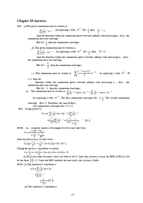
∞
−n
n =−∞
∑ (1/ 4)
∞
z −n zn
n =−3
∑ (1/ 4)
= ∑ (1/ 4) − n +3 z n −3
n=0
= (1/ 64) z −3 /(1 − 4 z ), z < 1/ 4 = (1/16) z −4 /(1 − (1/ 4) z −1 ), z < 1/ 4
The Fourier transform does not exist because the ROC includes the unit circle. (g) Consider x1 ( z ) = 2n μ[ − n].
X ( z) =
n =−∞
jw
r> 1 . The second summation
2
10.2
∑ ( 5 ) u[n − 3]z
n
∞
1
z −3 ∞ 1 n − n ]∑ ( ) z =[ 125 n = 0 5
∞ 1 = ∑ ( )n z − n n =3 5 z −3 1 ] =[ 125 1 − 1 z −1 5 −n
X ( Z ) = ∑ x[n]z − n
n =∞ ∞
−5
= ∑ (−1) n z − n
n =0
∞
= 1/(1 + z −1 ), z > 1
The Fourier transform does not exist because the ROC does not include the unit circle (d) For x [n]= ( 1 ) n +1 μ[n + 3],
x( z ) =
数字信号处理英文版课后答案 (4)
4.24 From the figure, the filter has a finite impulse response. It may be described as a sum of impulse function as: h[n] = 0.5[n] + 0.4[n–1] + 0.3[n–2] + 0.2[n–2] The difference equation has the parallel form: y[n] = 0.5x[n] + 0.4x[n–1] + 0.3x[n–2] + 0.2x[n–3] 4.25 n h[n] The impulse response is finite, with samples as listed in the table. 0 1.000 1 0.300 2 0.090 3 0.027 4 0.000 5 0.000 6 0.000
x[n]
+
delay –0.14 delay –0.38
y[n]
4.23 n h[n]
The first ten samples of the impulse response are: 0 1.0 1 –1.2 2 –0.8 3 0.4 4 0.0 5 0.0 6 0.0 7 0.0 8 0.0 9 0.0
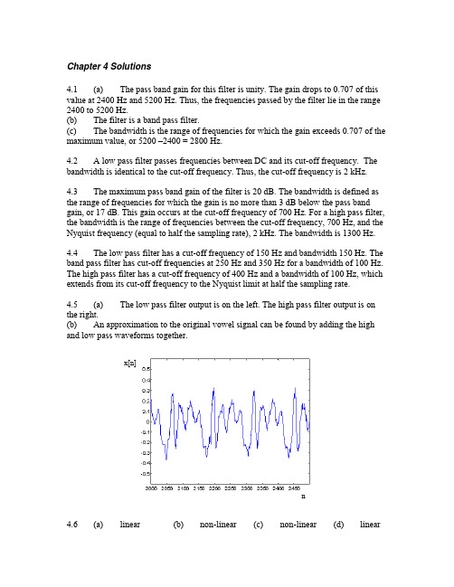
Chapter 4 Solutions 4.1 (a) The pass band gain for this filter is unity. The gain drops to 0.707 of this value at 2400 Hz and 5200 Hz. Thus, the frequencies passed by the filter lie in the range 2400 to 5200 Hz. (b) The filter is a band pass filter. (c) The bandwidth is the range of frequencies for which the gain exceeds 0.707 of the maximum value, or 5200 –2400 = 2800 Hz. 4.2 A low pass filter passes frequencies between DC and its cut-off frequency. The bandwidth is identical to the cut-off frequency. Thus, the cut-off frequency is 2 kHz. 4.3 The maximum pass band gain of the filter is 20 dB. The bandwidth is defined as the range of frequencies for which the gain is no more than 3 dB below the pass band gain, or 17 dB. This gain occurs at the cut-off frequency of 700 Hz. For a high pass filter, the bandwidth is the range of frequencies between the cut-off frequency, 700 Hz, and the Nyquist frequency (equal to half the sampling rate), 2 kHz. The bandwidth is 1300 Hz. 4.4 The low pass filter has a cut-off frequency of 150 Hz and bandwidth 150 Hz. The band pass filter has cut-off frequencies at 250 Hz and 350 Hz for a bandwidth of 100 Hz. The high pass filter has a cut-off frequency of 400 Hz and a bandwidth of 100 Hz, which extends from its cut-off frequency to the Nyquist limit at half the sampling rate. 4.5 (a) The low pass filter output is on the left. The high pass filter output is on the right. (b) An approximation to the original vowel signal can be found by adding the high and low pass waveforms together.
数字信号处理 英文版 课后习题
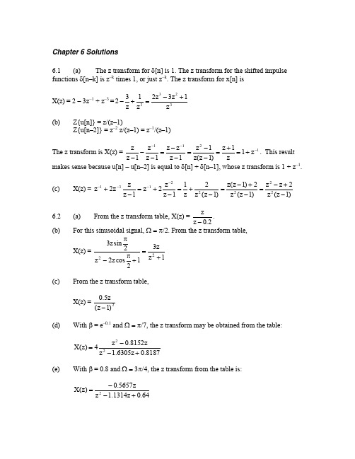
The difference equation can be found in two ways. By replacing h[n] with y[n] and [n] with x[n], the impulse response itself furnishes the difference equation y[n] = 2x[n] – 1.5x[n–1] + x[n–2] + 0.5x[n–3] Alternatively, the same difference equation can be found by using H(z) = Y(z)/X(z), cross-multiplying, and taking an inverse z transform. 6.9 n h[n] The samples of the impulse response are given in the table. 0 0.0 1 0.5625 2 0.3164 3 0.1780 4 0.0
The samples of the impulse responses are: 0 1.0 0.0 1 0.2 –3.0 2 0.04 –6.0 3 0.0 –9.0
The transfer functions of the systems are: H1(z) = 1 + 0.2z–1 + 0.04z–2 H2(z) = –3z–1 – 6z–2 – 9z–3 In cascade, the filters give the transfer function H(z) = H1(z)H2(z) = 3z 1 6.6z 2 10.32z 3 2.04z 4 0.36z 5 6.12 (b) 6.13 6.14
数字信号处理英文版课后答案(8)

Chapter 8 Solutions 8.1 The Fourier transform gives the spectrum of this non-periodic signal:Ω-Ω-++=Ω2j j e 25.0e 5.01)(X8.2 The samples for the signal are:The spectrum for the signal is given byΩ-Ω-Ω-++-=Ω4j 3j j e e e 5.0)(X8.3 Ω-Ω-Ω-Ω-∞-∞=Ω-++++==Ω∑8j 6j 4j 2j n jn e e e e 1e ]n [x )(X8.4 The first eight sample values for the signal are shown in the table.The signal contains an infinite number of non-zero samples, but the first 5, shown above, should be sufficient to approximate the DTFT reasonably well.Ω-Ω-Ω-Ω-∞-∞=Ω-+-+-≈=Ω∑4j 3j 2j j n jn e 0039.0e 0156.0e 0625.0e 25.01e ]n [x )(X8.5 The DTFT for x 1[n] isΩ-Ω-∞-∞=Ω-++==Ω∑2j j n jn 11e 3e 21e ]n [x )(XThe DTFT for x 2[n] isΩ-Ω-Ω-∞-∞=Ω-++==Ω∑4j 3j 2j n jn 22e 3e 2e 1e ]n [x )(XThe DTFT for x 3[n] isΩ-Ω-∞-∞=Ω-++==Ω∑2j j n jn 33e 1e 23e ]n [x )(XAll three signals have identical magnitude spectra, shown below.|X(The phase spectra of the three signals differ. They are shown in the figure below. From the DTFT expressions above, it is easy to see that )(X e )(X 12j 2Ω=ΩΩ- and)(X e )(X 12j 3Ω-=ΩΩ-. The first relationship means that the phase for x 2[n] will always be 2Ω less than the phase for x 1[n]. The second relationship means that the phase for x 3[n] is always 2Ω less than the negative of the phase for x 1[n], since X 1(-Ω) produces phases that are the negatives of the phases for X 1(Ω), following the odd phase spectrum rule. Both of these two relationships can be confirmed in the table or the plot, remembering that θ ± 2π = θ.8.6 The samples of the signal are shown in the table:The DTFT isΩ-Ω-Ω-∞-∞=Ω-+-==Ω∑4j 2j j n jn e 866.0e 866.0e 866.0e ]n [x )(X8.7 The period of the signal is N = 10. The sample values are listed in the table:The N = 10 DFS coefficients are given by:510k 2j 410k 2j 310k 2j 210k 2j 9n n10k 2j k e e e e e ]n [x c π-π-π-π-=π-+++==∑= 1|–2πk/5 + 1|–3πk/5 + 1|–4πk/5 + 1|–πkBecause of the symmetry of the spectrum, it is enough to calculate the coefficients for k = 0 to k = N/2 = 5, and to produce the other parts of the spectrum from this data.The magnitudes in the second half of the spectrum are a mirror image of those in the first. The phases in the second half are the negatives of the phases in the first half.|X(8.8 (a) The signal x[n] has the digital period N = 4. Its spectrum can be found using the discrete Fourier series:34k 2j 4k2j 3n n4k 2j k ee2e]n [x c π-π-=π--+==∑= 2 + 1|–πk/2 – 1|–3πk/2(b) The magnitude spectrum appears to repeat every second sample, while the phase spectrum repeats every four samples. The period of both spectra must be the same, so the overall period must be 4. As for all periodic signals, the period of the spectrum matches the period of the signal. 8.9 The signal has a period of N = 4, so the DFS coefficients are given by:24k2j 3n n4k 2j k e1e ]n [x c π-=π--==∑= 1 – 1|–πkSeveral cycles of the spectra are shown in the figures below.(8.10 The spectra for non-periodic signals are produced using the DTFT. The spectra, X(Ω), are smooth, continuous functions of frequency with a period of 2π. They are plotted against digital frequency Ω. If desired, the spectra can be plotted as X(f) versus frequency in Hz, using f = Ωf S /(2π).The spectra for periodic signals having a period N are produced using the DFS. The spectra, c k , are line functions of frequency with a period of N. They are plottedagainst the index k. If desired, the spectra can be plotted against frequency in Hz, using f = kf S /N.For both non-periodic and periodic signals, magnitude spectra are even and phase spectra are odd.8.11 (a) The signal is non-periodic. Its spectrum is given by the DTFT:Ω-Ω-Ω-∞-∞=Ω-++==Ω∑3j 2j j n jn e 3e 2e e ]n [x )(XThe magnitude and phase spectra appear as dashed lines in the figure in part (b). (b) The signal is a periodic version of the signal in (a), with period N = 4. Its spectrum is given by the DFS:34k2j 24k 2j 4k2j 3n n4k 2j k e3e 2ee]n [x c π-π-π-=π-++==∑= 1|–πk/2 + 2|–πk + 3|–3πk/2 The magnitude and phase spectrum are plotted below, dashed lines for the DTFT and solid for the DFS. Note that the DFS samples the DTFT.8.12 The harmonic frequencies are given by f = kf S /N. For f S = 12 kHz and N = 72, the first five harmonics are: 166.7, 333.3, 500.0, 666.7, and 833.3 Hz.8.13 For the first cosine, N/M = 2π/Ω = 2π/(2π/3) = 3, so the period is 3. For the second cosine, N/M = 2π/Ω = 2π/(π/3) = 6, so the period is 6. The lowest common multiple of these two periods is 6, so this is the overall period of the waveform.The signal samples are given by The Fourier coefficients are calculated as:56k2j 46k2j 36k2j 26k 2j 6k2j 5n n6k 2j k e5.0e 5.1e e 5.1e5.03e]n [x c π-π-π-π-π-=π---+--==∑= 3 – 0.5|–k π/3 –1.5|–2k π/3 + 1|–k π –1.5|–4k π/3 – 0.5|–5k π/3 The magnitude spectrum is periodic with period 6. Six spectrum samples cover the range from 0 to the sampling frequency, 4 kHz. Therefore, each point of the spectrum covers 4000/6 = 2000/3 Hz. As a result, k = 3 corresponds to the Nyquist frequency of 2 kHz. Using kf S /N, the two spikes in the spectrum below the Nyquist frequency, at k =1 and k = 2, map to frequencies of 2000/3 = 666.7 and 2(2000)/3 = 1333.3 Hz. Using Ω = 2πf/f S , these analog frequencies correspond to the digital frequencies π/3 and 2π/3 rads. Thespike at the higher frequency is twice the height of the other because its amplitude in the signal is double that of the other component. The other two spikes in the spectrum, at k = 6 – 1 and k = 6 – 2 map to imaged versions of the baseband frequencies.8.14 (a) Since the magnitude spectrum is periodic with period 14, the digital signal is periodic with the same period. (b) Fourteen points of the magnitude spectrum cover the sampling frequency, 16 kHz. Each point covers an interval 16/14 = 1.143 kHz wide. For a 16 kHz sampling frequency, the Nyquist frequency is 8 kHz. The first seven points of the magnitude spectrum cover this range. Three spikes occur within the Nyquist range, at k = 1, 2 and 3, or, using kf S /N, 1143, 2286 and 3429 Hz.(The magnitude spectrum belongs to the signal x[n] = sin(n π/7) + 2sin(n2π/7) +3sin(n3π/7). The digital frequencies π/7, 2π/7 and 3π/7 rads are, for a 16 kHz sampling rate, obtained from the analog frequencies 1143, 2286 and 3429 Hz.)8.15 (a) Since the magnitude spectrum has a period of 24, the digital signal also has a period of 24 samples. (b) Twenty-four samples cover 12 kHz, which means each point of the magnitude spectrum covers 0.5 kHz. The spikes at k = 2, 4 and 9 map to frequencies of kf S /N = 1, 2 and 4.5 kHz. The other three spikes are occur above the Nyquist frequency, at k = 24 –2 = 22, k = 24 – 4 = 20 and k = 24 – 9 = 15. The frequencies that correspond to these values of k are imaged copies of the baseband frequencies. (c) Using Ω = 2πf/f S , the digital frequencies are π/6, π/3 and 3π/4 rads.(The signal whose magnitude spectrum is shown is x[n] = cos(n π/6) + cos(n π/3) + cos(n3π/4).)8.16 The Fourier expansion can be matched to ∑-=π=1N 0k n N k2j k e c N 1]n [x . Since N = 16,n 1622j n1612j n 1612j n 1622j e e 2j 1e 2j e ]n [x πππ-π-+++-=⎪⎪⎭⎫ ⎝⎛+++-=πππ-π-n 1622j n 1612j n 1612j n 1622j e 8e 4j 8e 4j e 881The only non-zero coefficients c k are: c –2 = 8, c –1 = –j4, c 0 = 8, c 1 = j4, c 2 = 8. The other 11 coefficients in each period must be zero. The magnitudes of the non-zero coefficients are 8, 4, 8, 4, 8 and the phases are 0, –π/2, 0, π/2 and 0. The magnitude and phase spectra constructed using this information are shown below. Remember that the sequence of magnitudes and phases repeats every 16 points.8.17 (a)(i) Since 2π/Ω = 14π/(6π) = 7/3, the digital period is 7.(ii) The signal contains the frequency f = Ωf S /(2π) = 30000/7 Hz. For a digital period of 7, each point of the magnitude spectrum covers f S /N = 10000/7 Hz. Since each frequency is represented by kf S /N, a spike occurs in this magnitude spectrum at k = 3. Due to imaging, a second, symmetrically-placed spike occurs at N – 3 = 7 – 3 = 4.(b)(i) Since 2π/Ω = 10π/(3π) = 10/3, the digital period is 10.(ii) The signal contains the frequency f = Ωf S /(2π) = 3000 Hz. For a digital period of 10, each point of the magnitude spectrum covers f S /N = 1000 Hz. Therefore, a spike occurs in this magnitude spectrum at k = 3. Due to imaging, a second, symmetrically placed spike occurs at N – 3 = 10 – 3 = 7.(c)(i) For the first component 2π/Ω = 6, and for the second component 2π/Ω = 16. The digital period is the lowest common multiple of these two periods, or 48.(ii) The signal contains the frequencies f = Ωf S/(2π) = 10000/6 = 5000/3 Hz and f = Ωf S/(2π) = 10000/16 = 625 Hz. For a digital period of 48, each point of the magnitude spectrum covers f S/N = 10000/48 = 625/3 Hz. Therefore, spikes occur in this magnitude spectrum at k = 3 and k = 8. Symmetrically placed spikes occur at N – 3 = 48 – 3 = 45 and N – 8 = 48 – 8 = 40 as a result of imaging.(d)(i) As in part (c), the digital period is 48.(ii) The spikes occur in the same locations as in (c), but the higher frequency spike is twice as tall as the lower frequency spike.8.18 As evidenced by the zeros in the magnitude spectrum, some frequencies are excluded from this signal. The most significant contribution lies at a digital frequency of about 0.1 radian. The exact value is 0.113 radians. With f S = 20 kHz, f = Ωf S/(2π) = (0.113)(20000)/(2π), or about 360 Hz. The next biggest peak occurs at about 0.3 radians. The exact value is 0.336 radians, which corresponds to a frequency of 1070 Hz. Most of the important signal content lies below the fourth zero in the spectrum, at 0.395 radians or 1257 Hz.8.19 The number of points in the DFS spectrum gives the digital period of the underlying signal. The digital period in this case is N = 23. The periodic signal whose magnitude spectrum is shown has a large DC component and contributions at all harmonic frequencies, kf S/N = k(20000)/23 = 869.6k Hz. The first few harmonics are 869.6 Hz, 1739.1 Hz, 2608.7 Hz, …. The amplitudes of the harmonics decrease rapidly with frequency. The fundamental frequency of the signal is 869.6 Hz, so the period of the signal is NT S = 1.15 msec.8.20 (a) Ω-)X5.0(e5.0+Ωj-=(b) For a sampling frequency of f S= 16 kHz, the Nyquist frequency is 8 kHz. A cut-off of 2 kHz corresponds to a digital frequency of Ω = 2πf/f S = π/4 radians. The low pass filter extracts the lowest frequency elements in the signal.(c) Cut-off frequencies of 3 and 6 kHz correspond to digital frequencies of 0.375πand 0.75π radians. The band pass filter extracts the mid-range frequencies.(d) A cut-off of 7 kHz corresponds to a digital frequency of 0.875π radians. The high pass filter extracts only the highest frequency elements in the signal.8.21 (a) Each of the three terms is periodic. The digital period for each is 14, 3 and 16. The lowest common multiple for these integers is N = 336, the digital period for x[n]. The analog frequencies of the three terms are given by f = Ωf S/(2π). They are 1143, 5333, and 1000 Hz. The DFS frequencies are given by f = kf S/N = 47.6k, so the magnitude spectrum for the signal will contain peaks at k = 24, 112 and 21. These three peaks are shown below. Note the images of these peaks in the second half of the spectrum, at k = 363 – 21 = 342, k = 363 – 24 = 339, and k = 363 – 112 = 251.(b) The low pass filter will extract the two lowest-frequency peaks, at 1000 and 1143 Hz. The DFS magnitude spectrum will contain a peak at k = 21 and one at k = 24, plus imaged peaks at k = 363 – 21 = 342 and k = 363 – 24 = 339.(c) The band pass filter will extract the high frequency peak, at 5333 Hz. The DFS magnitude spectrum for the filtered output will contain a peak at k =112, plus an imaged peak at k = 363 – 112 = 251.(d) The high pass filter output will contain no peaks.8.22 (a) The spectrum has 64 points, so N = 64 is the digital period of the square wave. The fundamental frequency is f S/N = 4000/64 = 62.5 Hz.(b) The period in seconds is the reciprocal of the fundamental frequency, or NT S = 16 msec.(c) The DC component gives the average value of the signal. For this signal, the average is zero.(d) The harmonics present in the signal are odd multiples of the fundamental frequency. The only ones that lie below 500 Hz are 62.5k = 62.5, 187.5, 312.5, and 437.5 Hz. These frequencies correspond to the indices k = 1, 3, 5, 7.。
数字信号处理 英文版 课后习题
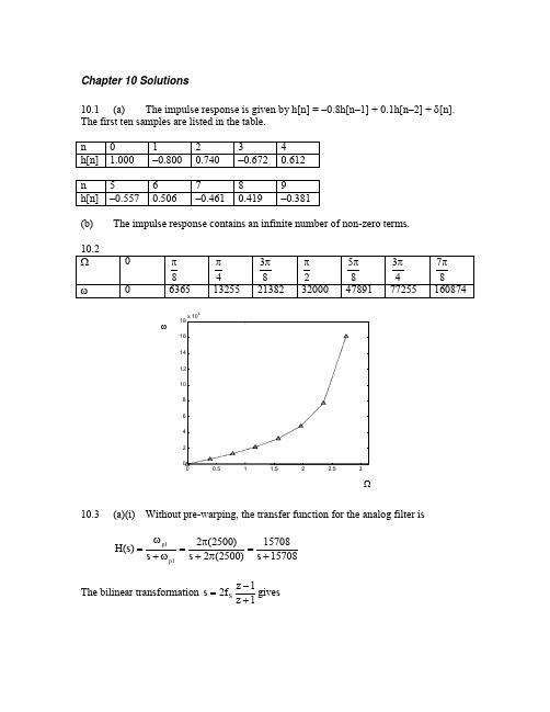
H(s)
p1 s p1
23946 s 23946
After the bilinear transformation, the digital transfer function is obtained:
H(z) 23946 0.6(1 z 1 ) z 1 1 0.1989z 1 16000 23946 z 1
: 2
The shape of the digital filter may be found by substituting 2f S tan
H ( )
1504.4 2 2f S tan 1504.4 2
2
1504.4 2 16000 tan 1504.4 2
(b)
Use the bilinear transformation to get the digital transfer function
1504.4 0.0859(1 z 1 ) H( z) z 1 1 0.8281z 1 16000 1504.4 z 1
The difference equation is y[n] = 0.8281y[n–1] + 0.0859x[n] + 0.0859x[n–1]. 0.0859(1 e j ) (d) The frequency response is H() . The magnitude response 1 0.8281e j may be found by taking the magnitudes of this expression for several values of . It is plotted below against frequency in Hz. (c)
数字信号处理(英文版)课后习题答案2
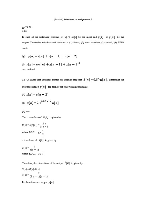
(Partial) Solutions to Assignment 2pp.73-761.16In each of the following systems, let or be the input and or be the output. Determine whether each systems is (1) linear, (2) time invariant, (3) causal, (4) BIBO stable(g).(i).ans: omitted----------------------------------------------------1.17 A linear time invariant system has impulse response Determine the output sequence for each of the followign input signals:(b)(f)(b) ans:h n is given byThe z-transform of []where ROC1:x n is given byz-transform of []where ROC2:h n is given byTherefore, the z-transform of the output []y nPerform inverse z to get [](f) ans: using the same method as in (b) (details omitted )----------------------------------------------------1.18. A linear time invariant system is defined by the difference equationb. Determine the output of the system when the intpu isc. Determine the output of the system when the input isans: omitted----------------------------------------------------1.19 The following expressions define linear time invariant systems. For each one determine the impulse respnose(a)(e)(a) ans: the impulse response is(e) ans: the impulse response is----------------------------------------------------1.20 Each of the following expressions defines a linear time invariant system. For each one determine whether it is BIBO stable or not(g)(k)BIBO: Bounded input and bounded output(g) ans: omitted(k) ans: omitted----------------------------------------------------1.21. Using the geometric series, for each of the following sequence determine the z-transform and its ROC(d)(g)(i)(d) ans:where ROC:(g) ans:The first part is equal towhere ROC1 isThe second part is equal towhere ROC2 isTherefore combining both parts:where ROC={ROC1 and ROC2}:(i) ans:where ROC: whole complex domain----------------------------------------------------1.22. You know what the and are. Using theproperties only (do not reuse the definition of the z-transform.) determine the z-transform of the following signals(c)(g)where ROC1:where ROC2:(c) ans: using z-transform property:We have:where ROC:(g) ans:details omitted. The final answer isTherefore combining both parts:where ROC={ROC1 and ROC2}:----------------------------------------------------1.23 Using partial fraction expansion, determine the inverse z-transform of the following functions:(c) ,(e) ,(c) ans:(e) ans:procedures are the same as above. details omitted.----------------------------------------------------1.24. For each of the followign linear difference equations, determine the impulse response, and indicate whether the system is BIBO stable or not(a)(c)(a) ans:Take z-transform on both sideswhere ROC:Because is finiteTherefore, the system is BIBO stable(c) ans: omitted (the same as (a))----------------------------------------------------1.25. Although most of the time we assume causality, a linear difference equation can be interpreted in a number of ways. Consider the linear difference equation(a) Determine the transfer function and the impulse response. Is the system causal ? BIBO stable ?(a) omitted.----------------------------------------------------1.26. 1.26 Consider the linear difference equation(a) Determine the transfer function . Do you have enough information to determine theregion of convergenceans:Don't have enough information to determine ROC.----------------------------------------------------1.27. Given the system described by the linear difference equationDetermine the output for each of the following input signals(a)(e)(a) ans:Take z-transform on both sides:----------------------------------------------------1.28. Repeat Problem 1.27 when the system is given in terms of the impulse responseBefore you do anything, is the system stable ? Does the frequency responseexist ?ans: omitted.----------------------------------------------------1.29. Repeat Problem 1.27 when the system isgiven by the linear difference equationBefore you do anything, is the system stable ? Does the frequency response exist ?Ans: omitted.----------------------------------------------------。
数字信号处理课后答案+第3章DFT+FFT
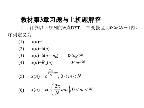
为x(n)=nRN(n), 所以 x(n)-x((n-1))NRN(n)+Nδ(n)=RN(n)
等式两边进行DFT, 得到
X(k)-X(k)WkN+N=Nδ(k)
故
X (k) N[δ(k) 1] 1 WNk
k 1, 2, , N 1
x9 (n) cos(0n) RN (n) Re[ x7 (n)]
X 9 (k )
X7e (k)
1 2[X7 (k)
X
* 7
(
N
k )]
1
1 e j0N
2
1
e
j(0
2π N
k
)
1 e j0N
1
e
j(0
2π N
)
k
(10) 解法一
N 1
X (k) nWNkn k 0, 1, , N 1 n0
x9 (n)cos(0n)RN
(n)
1 [e j0n 2
e j0n ]
X 9 (k)
N 1
x9 (n)WNkn
n0
1
N 1
[e j0n
e
j0
n
]e
j
2π N
k
n
2 n0
1
1 e j0N
2
1
e
j(0
2π N
k
)
1 e j0N
1 e
j(0
2π N
k
)
解法二 由DFT共轭对称性可得同样结果。 因为
W
k N
2WN2k
3WN3k
(N
1)WN( N 1)k
WNk X (k ) 0 WN2k 2WN3k 3WN4k (N 2)WN(N 1)k (N 1)
信号处理导论(英文影印版) 习题答案_9-11章
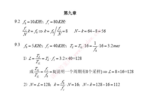
9.12⎥⎥⎥⎥⎦⎤⎢⎢⎢⎢⎣⎡=⎥⎥⎥⎥⎥⎥⎥⎥⎥⎥⎥⎦⎤⎢⎢⎢⎢⎢⎢⎢⎢⎢⎢⎢⎣⎡⎥⎥⎥⎥⎦⎤⎢⎢⎢⎢⎣⎡−−−−−−−−−−−−=0001221121221111111111111111111111111)1j j j j j j j j DFTdirect X 课后答案网ww w.kh da w.co m9.18或其它或或其它]2154300[]0154320[)2]154320[)1===x x x 本题考查两点基本概念:1)一序列先进行mod -N reduction 后再作N -point DFT 与其直接作N -point DFT 结果相等。
2)不同序列有可能有相同的mod -N reduction 结果课后答案网ww w.kh da w.co m9.30碟形图见黑板))2]28682868[~]3101124211781744[1−−=−−−−−=∗=y h x y 课后答案网ww w.kh da w.co m9.41]1010101010120202020101[]1010101010120202020101[]00010201[~],10101212[~],01012121[~],02020202[~],20101323[~]00000011[]01111222[]22221113[]11333311[]31111000[333],1111[h 8815432154321−−−−−−=∗=−−−−−−=−=−−−=−−−=−−=−−=⎪⎪⎪⎩⎪⎪⎪⎨⎧=====∴=∴−−=∴−−h x y y y y y y y x x x x x M ns convolutio circular length methodsave overlap ,即每段间重叠阶数为每段长度取要做)Q Q 课后答案网ww w.kh da w.co m]1010101010120202020101[]01010101[~],20201111[~],10102303[~],32320101[~]01111[]22221[],11333[],31111[5x (888)241443322114321−−−−−−=−−==−−−==−−==−−−=======∴≤+≤∴−−y y y y y y y y y y y x x x x y 重叠相加得到以上取为滤波器阶数)的长度,为每子段即每段卷积输出长度要做N M N M N L ns convolutio circular length methodadd overlap i Q 课后答案网ww w.kh da w.co m)()()()()()3()()()()()()()()()()()()()()2()()()()()(ωωωωωωωωωωωωωωωω−===−∴−=−=−==−∴−=−=−==∑∑∑∑∑∑∑∑∞+−∞=−−∞+−∞=∗∞+−∞=−∞+−∞=−−=∞+−∞=∞+−∞=−∞+−∞=−−=∞+−∞=∗D ek d ek d D symmetrynot butvalue real only is k d oddis D D el d el d ek d D imaginaryis D D el d el d ek d D realandodd is k d k kj k kj k d l lj k d l lj l k k kj l lj k d l lj l k k kj k d 为实数为奇函数为奇函数为实数课后答案网 ww w.kh da w.co m。
数字信号处理(英文版)课后习题答案
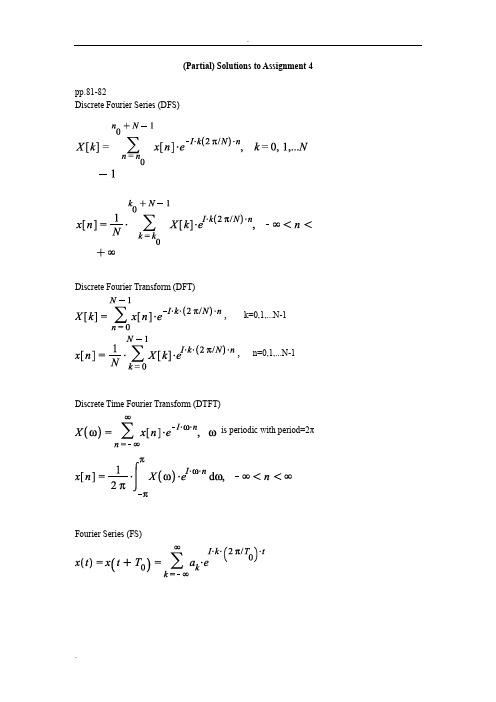
(Partial) Solutions to Assignment 4pp.81-82Discrete Fourier Series (DFS)Discrete Fourier Transform (DFT), k=0,1,...N-1, n=0,1,...N-1Discrete Time Fourier Transform (DTFT)is periodic with period=2πFourier Series (FS)Fourier Transform (FT)---------------------------------------------------- 2.1 Consider a sinusoidal signalQ2.1 Consider a sinusoidal signalthat is sampled at a frequency s F =2 kHza). Determine an expressoin for the sampled sequence , and determine itsdiscrete time Fourier transformb) Determinec) Re-compute ()X from ()X F and verify that you obtain the same expression as in (a)a). ans:=where andUsing the formular:b) ans:wherec). ans:Let be the sample function. The Fourier transform of isUsing the relationship orwhereConsider only the region where ( orthereforewhereEND-----------------------------2.3 For each shown, determine whereis the sampled sequence. The sampling frequence is given for each case.(b) Hz(d) Hztheory: the relationship between DTFT and FT iswhereorb. ans:d. ans:omitted (using the same method as above)----------------------------------------------------2.4 In the system shown, let the sequence be and the sampling frequency be kHz. Also let the lowpass filter be ideal, with bandwidth (a). Determine an expression for Also sketch the frequency spectrum (magnitude only) within the frequency range(b) Determine the output signal(a) ansFrom class notes, we have where is an ZOH interpolation function and We can writeFirstly, to findwhereIt can be found asSecondly, find This can be solved either by FT or DTFT.We can writewhere andUsing the formula:we haveUsing the formula,:we have from DTFT of y[n]Note the above expression is two pulses at and -the scaling factor is:whereTherefore,where(b) ans:After the ideal LPF, the Fourier transform ofTake inverse Fourier transform of , the output signal is:Note both the and θ terms are introduced by ZOH functionwhere is introduced because is non-ideal and θ represents the delay of----------------------------------------------------Q 2.5. We want to digitize and store a signal on a CD, and then reconstruct it at a later time. Let the signaland let the sampling frequency Hz.(a) Determine the continuous time signal after the reconstruction.(a) ans: Assuming (ZOH+ ideal LPF) is used. This problem can be solved by using the results directly from Q2.4. In Q2.5 there are 3 sinusoidal signals instead of only one in Q2.4. Details of the solutions are omitted.----------------------------------------------------Q 2.6 In the system shown, determine the output signal for each of the following input signal Assume the sampling frequency kHz and the low pass filter (LPF) to beideal, with bandwidth(b)(d)Ans (b) (d): same as in problem Q2.5.----------------------------------------------------2.7 Suppose in DAC you want to use a linear interpolation between samples, as shown in the accompanying figure. This reconstructor can be called a first order hold, because the equation of a line is a polynomial of degree 1(a). Show that with a triangular pulse as shownin the figure(b). Determine an expression for in terms ofand(c). In the accompanying figure, let kHz, and the filterbe ideal with bandwidth Determine the outputAns: omitted.----------------------------------------------------2.9 In the following system, let the signal be affected by some random error as shown. The error is white, zero mean, with variance Determine the variance of the error after the filter for each of the filter(b)(b) ans:The variance of the output of the filter is given byTherefore--------------------------------------------------------------------------------------------------------------------------------------------------------------------------------------------------------------------------------------------------------------------------------------------------------------------------------------------------------------------------------------------------------------------------------。
数字信号处理课后答案
⎣⎢y[3]⎦⎥ ⎣⎢1 − j −1 j ⎦⎥ ⎣⎢2 + j⎦⎥ ⎣⎢ 2 ⎦⎥
5.56 Similarly to the solution of Problem 5.55, we first calculate the DFT X[k] of x[n]: €
⎡X[0]⎤ ⎡1 1 1 1 ⎤ ⎡ 1 ⎤ ⎡ 2 ⎤
2
5.54 €
(a)
Given:
y[n] = αg[n] + βh[n]. Therefore:
Y[k]
=
N −1
∑
y[n]W
nk N
n=0
=
α
N −1
∑
g[n]WNnk
+
β
N −1
∑
h[n]WNnk
=
αG[k] +
βH[k].
€
n=0
n=0
€
(b) Given: x[n] = g[〈n − no〉N ]. Therefore:
∑ x[n]
y[〈
+
n〉
N
⎞ ⎟ W
k N
€
=0
=0⎝ n=0 €
⎠
=
N −1
∑
n=0
⎛N −1 x[n]⎜ ∑
⎝ =0
y[〈
+
n〉
N
]WNk
⎞ ⎟ ⎠
=
N −1
∑
n=0
⎛ x[n]⎜
⎝
N −1
∑
=0
y[m]W
(m−n) N
⎞ ⎟ ⎠
€
=
N −1
k
−
m2
〉
数字信号处理英文版课后答案(3)
Chapter 3 Solutions3.1 (a) (i) x[0] = 3(ii) x[3] = 5(iii) x[–1] = 2(b) (i)(ii) The sketch for x[n+1] does not show the value of the sample x[5], since this information is not provided in the question.3.2 The impulse function is zero everywhere except n = 0.(a) δ[–4] = 0(b) δ[0] = 1(c) δ[2] = 03.3 (a) This function is a mirror image of the impulse function across the verticalaxis, which means no change occurs.(b) This function shifts the impulse two steps to the right and increases its amplitude to 2.(c) This function is the sum of two impulse functions.3.4 The step function is zero for n < 0 and one everywhere else.(a) u[–3] = 0(b) u[0] = 1(c) u[2] = 13.5 (a) x[n] = 4u[n–1](b) x[n] = –2u[n](c) x[n] = 2u[–n](d) x[n] = u[n–2](e) x[n] = u[2–n]3.6(a)(b)3.7 (a) This signal is a sum of shifted step functions, each with amplitude one. x[n] = 0.1u[n –1] + 0.1u[n –2] + 0.1u[n –3] + …(b) This signal is a sum of impulse functions with increasing amplitude. x[n] = 0.1δ[n –1] + 0.2δ[n –2] + 0.3δ[n –3] + …3.8 x[n] = (u[n] – u[n –2]) + (u[n –5] – u[n –7]) + (u[n –10] – u[n –12])3.9 x[n] = 2δ[n] – 3δ[n –1] + δ[n –2] – δ[n –3] + 3δ[n –4]3.10 (a)x[n] = δ[n –3] + δ[n –4] + δ[n –5] + δ[n –6] – δ[n –7] – δ[n –8] – δ[n –9] – δ[n –10] – δ[n –11] ∑∑==-δ--δ=117k 63k ]k n []k n [(b) x[n] = u[n –3] – 2u[n –7] + u[n –12] 3.11 x[n] = u[n] + 2u[n –4]3.123.13 The signal has values 1, 0.5, 0.25, 0.125, etc. These values can be generated from the function 0.5n , where each value is the amplitude of an impulse function. The signal may be expressed as ∑∞=-δ=0k k ]k n [)5.0(]n [x = δ[n] + 0.5δ[n –1] + 0.25δ[n –2] + 0.125δ[n –3] + …3.14 (a)By Euler’s identity, ⎪⎭⎫ ⎝⎛π-⎪⎭⎫ ⎝⎛π==π-4n sin j 4n cos e]n [x 4n j(b)From (a), 4π=Ω. Therefore, 18422=ππ=Ωπ. The digital period is 8 samples.3.15 (a)⎪⎭⎫⎝⎛π-⎪⎭⎫ ⎝⎛π==π-3n sin j 3n cos e ]n [x 3n j(b) The magnitude of any complex number is the square root of the sum of the squares of the real and imaginary parts. The magnitudes in the last column in (a) show that 3n j eπ- = 1. This equation is true for all n.3.16 The frequency of the analog signal is f = ω/2π = 200/2π Hz. The samplingfrequency f S = 1/T S = 1/(25x10–3) = 40 Hz. The digital frequency is Ω = 2πf/f S = 200/40 = 5 rads. The sampled signal is x[n] = 5sin(n Ω) = 5sin(5n).3.17 Check 2π/Ω for each function. The function is periodic if this ratio is rational. (a) 2π/Ω = 2π/(4/5) = 10π/4 = 5π/2This ratio is not rational, so the sinusoid is not periodic. (b) 2π/Ω = 2π/(6π/7) = 14/6 = 7/3This ratio is rational, and in lowest terms. The number in the numerator, 7, is the number of samples before the sequence repeats. (c) 2π/Ω = 2π/(2π/3) = 3This result may be seen as 3/1. Thus, the sinusoid is periodic with period 3.3.18 (a) From the equation for x(t), ω = 2πf = 1000π, so f = 500 Hz. Since seven samples are collected every three cycles, N = 7 and M = 3, so37M N 2==ΩπThis means SS f 5002f f 276π=π=π=Ω. Solving S f 500276π=π gives f S = 1167 Hz. (b) Since f S > 2f, the sampling rate is adequate to avoid aliasing.3.19 (a) The following samples are graphed below.(b) The ratio 2π/Ω is 2π/(4π/5)=10/4 = 5/2. The numerator, 5, indicates the sinusoidal sequence repeats every five samples. Because the denominator of the ratio is 2, these five samples are collected over two analog periods.(c) The analog signal is superimposed over the digital signal with a dashed line in the figure below.3.20 The analog frequency of x(t) is f = ω/(2π) = 2500π/(2π) = 1250 Hz. The digital frequency of x[n] is π/3 radians. These frequencies must be related through the equationSS f 12502f f 23π=π=π=ΩThe solution to this equation is f S = 7500 Hz. One other solution is possible, since⎪⎭⎫⎝⎛π=⎪⎭⎫ ⎝⎛π-π=⎪⎭⎫ ⎝⎛π3n 5cos 3n n 2cos 3n cos . This view givesSf 1250235π=π=Ωor f S = 1500 Hz. At this frequency, aliasing occurs. The signal appears at a frequency of 250 Hz. This explains why this second sampling rate works:315002502f f 2S π=π=π=Ω3.21 (a) From 052n 92=π+π, n = 59-. The shift moves the function left by 9/5samples. (b) The samples in the two signals do not match, because the shift is not an integer.(c) 951.052)0(92sin ]0[x 1=⎪⎭⎫ ⎝⎛π+π=927.052)1(92sin ]1[x 1=⎪⎭⎫ ⎝⎛π+π=(d) For a phase shift of two samples to the right,0)2(92n 92=θ+π=θ+π, so 94π-=θ. Thus, ⎪⎭⎫ ⎝⎛π-π=94n 92sin ]n [x 1. One period of this signal contains the same sample values as one period of x 2[n]. 3.22 (a)(b)(c)(d) 3.23(a)Since the digital sinusoid is periodic,M 10M N 2==Ωπ. Since Sf f 2π=Ω, M10f f S =. Therefore, 10Mf f S=. Possible frequencies f of the analog signal are defined by M = 1, 3, 7, 9, 11, …, that is, all integers that do not share any factors with 10. Other integers M result in a digital period less than 10. For 4 kHz sampling, the possible frequencies f are 400, 1200, 2800, 3600, 4400, … Hz. (b) The only two frequencies from (a) that lie within the Nyquist range are 400 Hz and 1200 Hz. All other frequencies f, when sampled at 4 kHz, produce aliases at 400 or 1200 Hz.3.24 A 16-bit image uses 16 bits to represent the gray scale level for each pixel in the image. A total of 65,536 gray scale values can be represented with 16 bits.3.25 Each square on the checkerboard is recorded by a 16 x 16 block of pixels. All pixels in the white squares have gray scale value 255. All pixels in the black squares have gray scale value 0.。
数字信号处理教程课后习题及答案

解:(1 )
n
y(n) = ∑ x(m ) m = −∞
n
y1 (n ) = T [x1 (n )] = ∑ x1 (m ) m = −∞
y2 (n ) = T [x2 (n )] =
n
∑ x2 (m )
m = −∞
n
ay1(n)+ by2 (n) = ∑[ax1(m) + bx2 (n)] m = −∞
β α
n +1
β α β =
n +1− N −n0
N−
N
α −β
y(n) = Nα n−n0 ,
(α = β )
, (α ≠ β )
如此题所示,因而要分段求解。
2 .已知线性移不变系统的输入为 x( n ) ,系统的单位抽样响应
为 h( n ) ,试求系统的输出 y( n ) ,并画图。
(1)x(n) = δ (n)
=
x(n)sin⎜⎝⎛
2π 9
+
π 7
⎟⎠⎞
ay1(n)+ by2 (n)
=
ax1(n
)
sin(
2π 9
+
π 7
)
+
bx2
(n)
sin(
2π 9
+
π 7
)
7. 试判断以下每一系统是否是(1)线性,(2)移不变的?
( ) T[x(n
−
m )] =
x(n
−
m)sin
2π 9
+
π 7
( ) y(n
− m)=
4
第一章 离散时间信号与系统
1 .直接计算下面两个序列的卷积和 y( n ) = x( n )* h( n )
数字信号处理英文版课后答案 (9)

0 0.0 0
/8 –2.9 –68
/4 3/8 –16.9 –14.5 –135 –12
/2 –16.9 –90
5/8 –20.5 23
|H()|
()
100
50
0
-50
-100
-150 0 0.5 1 1.5 2 2.5 3
(b) In the pass band, which lies within the first “bump” of the magnitude spectrum, the phase spectrum follows a straight line. This means the phase is linear in this region, which in turn means that no distortion will occur. 9.4 (a)
h 1 [n ]
The sample values are given in the table. Note that at n = 0, it is easiest to evaluate h1[n] if it is re-expressed as
h 1 [n ] 0.5n sin 0.5n 0.5 sinc0.5n ) n 0.5n
y[n ]
The difference equation for a three-term moving average filter is
1 x[n] x[n 1] x[n 2] 3
The filter finds the average of each group of three input samples. The first sixteen outputs are: n y[n] n y[n] 0 3.33 8 1.00 1 3.67 9 1.00 2 4.00 10 1.00 3 1.00 11 4.00 4 1.00 12 4.00 5 1.00 13 4.00 6 1.00 14 1.00 7 1.00 15 1.00
数字信号处理(英文版)复习重点题型和答案

b. (omit)
pp76 Q1.13 Given the discrete time sinusoid x[n] = 2cos(0.2π n + 0.1π ) and the sampling frequency Fs = 2 kHz a. Determine the corresponding continuous time sinusoid in the frequency range 0 < F0 < F / 2 b. Determine two other continuous time sinusoids with the same sample values
⎞ ⎟ X [k ] ⎠
, where X [k ] are computed in the previous question.
b. x[n] = u[n − 2] Ans:
y[n] = h[n] ∗ x[n] = ∑ h[n − k ]x[k ] = ∑ 0.5n−k u[ n − k ]u[ k − 2]
k k
Since u[n] = 0 for n < 0 , u[n − k ] ≠ 0 for k ≤ n , and u[k − 2] ≠ 0 for k ≥ 2 Therefore, when n < 2 , y[n] = 0 . When n ≥ 2
Ans. a. x[n] = 2cos(0.2π n + 0.1π ) Digital frequency: ω0 = 0.2π = 2π F0Ts Therefore, the continuous time frequency:
F0 =
ω0 0.2π 2 = 0.2 kHz = 2π Ts 2π
数字信号处理 Mitra 第三版 答案
4.
Page 290, Problem 5.12:
Replace
“
x1[n]
=
⎜⎝⎛
x[n]
+
x[
N 2
+ n]⎟⎠⎞WNn ” with
“
x1[n]
=
⎜⎝⎛ x[n] −
x[ N
2
+
n] ⎟⎠⎞ WNn
”.
5.
Page 291, Problem 5.15: Replace “ h[n] = ⎩⎨⎧x[0n,],
3. Page 418, Problem 7.53: Replace “ − j0.3 ” with “ − j ”.
4. Page 421, Problem 7.79: Replace “ 0.5 − 0.4z −1 + 0.8z −2 + 0.8z −3 − 0.4z −4 + 0.5z −5 ” with “ − 0.1 + 0.5z −1 + 0.05z −2 + 0.05z −3 + 0.5z −4 − 0.1z −5 ”.
4.
Page 161, Problem 3.6(d):
Replace
“
X
a
⎜⎛ ⎝
Ω a
⎟⎞ ⎠
”
with
“
X
a
⎜⎛ ⎝
j
Ω a
⎟⎞ ⎠
”.
5. Page 162, Problem 3.16: Replace “1.. ” with “1. ”.
1
6.
Page 163, Problem 3.21(d):
12. Page 167, Problem 3.61(d): Replace “ Hb (e jω ) ” with “ Hd (e jω ) ”.
数字信号处理英文版课后答案 (2)
0
10
20
30
40
50
60
70
80
90 100 110 120 130 140 150
Frequency, kHz
(b) The sampling rate is too low for this signal, so aliasing occurs. Spectral images are shown by dashed lines, while the final spectrum is shown as a solid line.
0
10
20
30
ห้องสมุดไป่ตู้
40
50
60
70
80
90 100 110 120 130 140 150
Frequency, kHz
2.8 The cell phone signal is band-limited. The transmission range is 30 kHz wide. The minimum sampling rate must be at least 60 kHz. In this case, a 60 kHz sampling rate is adequate. A baseband copy of the transmission can be recovered by a filter with a 30 kHz cut-off.
2.13 Since images of the target appear at 0 0.2 MHz, 2 0.2 MHz, 4 0.2 MHz, … 900 0.2 MHz, the actual frequency of the target is 900.2 MHz. 2.14 In each revolution of the wheel, the tire covers d = .635 = 1.995 m. The bicycle travels 15 km/h, or 15000/3600 = 4.17 m/sec. Thus, each tire of the bicycle revolves at 4.17 m/sec the rate of 2.09 cycles/sec . According to Nyquist, at least two samples 1.995 m/cycle must be taken per cycle, for a sampling rate of 4.18 samples/sec. This can be accomplished by taking 418 snapshots in every 100 seconds. 2.15 When the signal is sampled at 600 Hz, images of the sine wave’s frequency on either side of every multiple of the sampling frequency. Since the aliased frequency is 150 Hz, copies appear at 0 ±150, 600 ±150, 1200 ±150, etc. Only 150, 450 and 750 Hz lie below 1 kHz. When the sampling rate is 550 Hz, the aliased frequency is 200 Hz, so copies must appear at 0 ± 50, 550 ±200, 1100 ±200, etc. Only 200, 350, 750 and 900 Hz lie below 1 kHz. The only sine wave that is consistent with both sampling results has a frequency of 750 Hz. 2.16 (a) (b) (c) 2.17 The range of analog voltages is 6 V. quantization step = 6/24 = 375 mV quantization step = 6/28 = 23.44 mV quantization step = 6/216 = 91.55 V (a) 28 = 256 (b) 210 = 1024 (c) 212 = 4096
数字信号处理第10章习题

第十章习题10-1. 试证明随即过程统计平均量的下列性质: (a) ][][][m n m n y E x E y x E +=+ (b)][][n n x aE ax E =【解题思路】从定义去证明。
证明:(a)][][),(),(),(),(),,,(),,,(),,,(),,,(),,,(),,,()(][22m n y x x x y y x y x y x y x y x y x m n y E x E dy m y yp dx n x xp n x p xn x P yx m y n x P dyy x m y n x P dy m y n x p dxdym y n x yp dxdy m y n x xp dxdym y n x p y x y x E m n n n m n m n m n m n m n m n +=+∴=∂∂=∂∂∂=∂∂∂=+=+=+⎰⎰⎰⎰⎰⎰⎰⎰⎰⎰∞+∞-∞+∞-∞+-∞=∞+∞-∞+∞-∞+∞-∞+∞-∞+∞-∞+∞-+∞∞-+∞∞-上式=(b)][),(),(][n x x n x aE dx n x xp a dx n x axp ax E n n ===⎰⎰+∞∞-+∞∞-10-2. 设x(n)和y(n)是两不相关的随机序列,试证: 如果w(n)=x(n)+y(n),则y x μμμω+=和222y x σσσω+=【解题思路】从定义去证明。
证明:yx w y x n y E n x E n y n x E n w E n y E u n x E μμμμ+=+=+==∴==)]([)]([)]()([)]([)]([)]([用上题结论])()))(()((2))()([(])))()([(]))([(]))([(]))([(222222222y x y x y x w w y y x x n y n x n y n x E n y n x E n w E n y E n x E μμμμμμμσμσμσ++++-+=--+=-=∴-=-= 又证明:2)()]}([)]([){()]()([)()]))(()([(y x y x y x y x n y E n x E n y n x E n y n x E μμμμμμμμ+=++=++=++222222222222222222])([])([])(2)()([)]([)]([)]()([)()()]()([2)]([)]([]))()([()(]))()([(])())()([(yx y x y x y x w yx y x y x w n y E n x E n y n x E n y E n x E n y n x E n y n x n y n x E n y E n x E n y n x E n y n x E n y n x E σσμμμμμμσμμμμμμσ+=-+-=+-++=∴=⋅∴++++-+=+-+=∴=不相关与由于=其中10-3. 某一个随机过程的取样序列x(n)的形式为)cos()(0θω+=n n x式中θ是一个均匀分布的随机变量,其概率密度如图。
- 1、下载文档前请自行甄别文档内容的完整性,平台不提供额外的编辑、内容补充、找答案等附加服务。
- 2、"仅部分预览"的文档,不可在线预览部分如存在完整性等问题,可反馈申请退款(可完整预览的文档不适用该条件!)。
- 3、如文档侵犯您的权益,请联系客服反馈,我们会尽快为您处理(人工客服工作时间:9:00-18:30)。
f p1 fS
2
6500 0.542 radians 24000
s1 = 2
f s1 8000 2 0.667 radians fS 24000
|H()|
1 0.9 0.8 0.7 0.6 0.5 0.4 0.3 0.2 0.1 0 0 0.5 1 1.5 2 2.5 3
10.5 The –3 dB frequency for this filter is 1 kHz. This is the edge of the pass band. The stop band edge can chosen at any convenient place. For example, the gain at 3 kHz is about –46 dB. The stop band ripple is given by 20logs = –46, or s = 0.005. The digital frequencies at the edges of the pass band and stop band are p1 = 2
p1 2 23946 rad/sec
p1 = 2f S tan s1 = 2f S tan
s1 203299 rad/sec 2
The order for the filter can be calculated using
1 1 log log 1 2 (0.01778) 2 1 s 1.9 n 203299 2 log 2 log s1 23946 p 1
7 8 160874
0
0.5
1
1.5
2
2.5
3
10.3
(a)(i) Without pre-warping, the transfer function for the analog filter is
H(s)
p1 s p1
2(2500) 15708 s 2(2500) s 15708
p1 2 54791.4 rad/sec
p1 = 2f S tan s1 = 2f S tan
s1 83239.1 rad/sec 2
The order for the filter can be calculated using
1 1 log 2 1 log (0.0398) 2 1 s 7.7 n 83239.1 2 log 2 log s1 p1 54791.4
Filter without pre-warping
f
10.4 (a) The cut-off frequency for the analog filter is 1500/(2) = 238.73 Hz. The digital frequency that corresponds to this analog frequency is p1 = 2(238.73) / 8000 = p1 0.1875 rads. The pre-warped analog cut-off frequency is p1 2f S tan = 1504.4 2 1504.4 rad/sec, to give the transfer function H(s) . s 1504.4
16
The plot of |H()| versus is the same as the plot of |H(f)| versus f, except that, along the horizontal axis, digital frequencies between 0 and radians are converted to frequencies between 0 and 12000 Hz (half the sampling rate). The magnitude response is shown below. The eighth order filter matches the specifications.
so an order of 2 should be chosen. 10.8 The 600 Hz transition width puts the stop band edge at 1.9 kHz. The digital pass band edge frequencies are p1 = 2
The order for the filter is
1 1 log 2 1 log (0.005) 2 1 s 3 n 38627.4 2 log 2 log s1 6627.4 p1
The bilinear transformation s 2f S
z 1 gives z 1
H( z)
15708 0.4954(1 z 1 ) z 1 1 0.00921z 1 16000 15708 z 1
(ii) The analog frequency 2.5 kHz is converted to a digital frequency p1 = 2(2500) / 8000 =1.9635 rads. This frequency is pre-warped to the analog frequency p1 = 23946 rad/sec, which makes the transfer function for the analog filter p1 2f S tan 2
(b) The magnitude responses for both filters are shown below. The –3 dB frequency for the pre-warped filter is equal to the specified 2.5 kHz.
|H(f)| Filter with pre-warping
The impulse response contains an infinite number of non-zero terms. 0 0
8 6365
18 16 14 12 10 8 6 4 2 0 x 10
4
4 13255
3 8 21382
2 32000
5 8 47891
3 4 77255
: 2
The shape of the digital filter may be found by substituting 2f S tan
H ( )
1504.4 2 2f S tan 1504.4 2
2
1504.4 2 16000 tan 1504.4 2
(b)
Use the bilinear transformation to get the digital transfer function
1504.4 0.0859(1 z 1 ) H( z) z 1 1 0.8281z 1 16000 1504.4 z 1
The difference equation is y[n] = 0.8281y[n–1] + 0.0859x[n] + 0.0859x[n–1]. 0.0859(1 e j ) (d) The frequency response is H() . The magnitude response 1 0.8281e j may be found by taking the magnitudes of this expression for several values of . It is plotted below against frequency in Hz. (c)
|H(f)|
1 0.9 0.8 0.7 0.6 0.5 0.4 0ቤተ መጻሕፍቲ ባይዱ3 0.2 0.1 0 0 500 1000 1500 2000 2500 3000 3500 4000
f
(e)
The magnitude for the analog transfer function is
H()
1504.4 2 1504.4 2
2
This function may be plotted for various values of . The magnitude response is plotted below against digital frequency in rads. When digital frequencies are converted to frequencies in Hz, the plot becomes identical to the one in part (d).
f p1 fS
2
1000 0.25 radians 8000
s1 = 2
f s1 3000 2 0.75 radians fS 8000
p1 2 6627.4 rad/sec
p1 = 2f S tan
s1 = 2f S tan
s1 38627.4 rad/sec 2
H(s)
p1 s p1
23946 s 23946
After the bilinear transformation, the digital transfer function is obtained:
H(z)
23946 0.6(1 z 1 ) z 1 1 0.1989z 1 16000 23946 z 1
