斯坦福大学机器学习课程个人笔记完整版
cs229斯坦福大学机器学习教程 Supplemental notes 4 - hoeffding

John Duchi
1
Basic probability bounds
A basic question in probability, statistics, and machine learning is the following: given a random variable Z with expectation E[Z ], how likely is Z to be close to its expectation? And more precisely, how close is it likely to be? With that in mind, these notes give a few tools for computing bounds of the form P(Z ≥ E[Z ] + t) and P(Z ≤ E[Z ] − t) (1)
for t ≥ 0. Our first bound is perhaps the most basic of all probability inequalities, and it is known as Markov’s inequality. Given its basic-ness, it is perhaps unsurprising that its proof is essentially only one line. Proposition 1 (Markov’s inequality). Let Z ≥ 0 be a non-negative random variable. Then for all t ≥ 0, P( Z ≥ t ) ≤ E [Z ] . t
斯坦福机器学习公开课笔记_ml-8 机器学习系统设计

斯坦福机器学习公开课(八)--机器学习系统设计公开课地址:https:///ml-003/class/index授课老师:Andrew Ng1、prioritizing what to work on:spam classification example(垃圾邮件分类系统)前面学到的都是一些理论知识外加实践过程中的诊断方法,这一讲是针对一个实际问题进行分析-垃圾邮件分类系统。
相信大部分用过email的人都知道什么是垃圾邮件,对垃圾邮件也深恶痛觉,如果不知道什么是垃圾邮件的请看下面:左边很明显是一个垃圾邮件,先看发送邮箱诡异的名字,再看发送内容中各种拼写错误的单词,估计就知道这肯定不是人写的而是电脑产生的了。
相比之下右边的邮件就是非垃圾邮件。
为了区别出垃圾邮件,首先要做的应该是寻找一些可以标记什么是垃圾邮件的特征,找到这些特征以后,再进行有监督的分类就能把垃圾邮件找出来了。
至于特征,我们可以从单词入手:如上所示,可以选择出现频率最高的100个单词作为候选集,得到一个100维的向量,然后从垃圾邮件中查看是否出现这些单词,如果出现就把对应位置标记为1,这样每一封垃圾邮件都能对应一个100维的向量。
不过如果要更精确一些,100个单词显然是不够的。
为了提高准确率,可以采用下面几种方法:翻译过来是:收集大量数据,显然的从邮件路由信息着手建立较为复杂的特征,诸如发件者邮箱对邮件正文建立复杂精确的特征库,例如是否应把discount和discounts视作同一个词等建立算法检查拼写错误,例如针对med1cine这样拼写错误的词2、error analysis(错误分析)既然知道了该怎么做,那接下来就是行动了。
这里Andrew Ng教授给出了他自己的见解:翻译过来如下:尽可能快的实现一个简单的算法,无论是逻辑回归还是线性回归也好,先利用简单的特征,然后在验证数据集上进行测试;利用画学习曲线的方法去研究是增加数据还是增加特征对系统更有利错误分析:人工去查看是哪些数据造成了错误的产生,错误的产生和样本之间是否存在一种趋势?在进行简单的算法实现和验证后,我们对模型做错误分析可以把垃圾邮件再分为四类(Pharma,Replica/fake,Steal passwords,Other):现在可以考虑针对一些词的不同形式是不是该看成一样的,这里不应该主观的去想当然,而是通过比较错误率来确定,例如下面就是针对discount这个词的各种变形判断是不是应该看成是一个词:3、error metrics for skewed classes(倾斜类误差度量)什么是Skewed Classes呢?一个分类问题,如果结果仅有两类y=0和y=1,而且其中一类样本非常多,另一类非常少,我们称这种分类问题中的类为Skewed Classes. 可以举个例子,如果要判断病人是否患癌症,假设采用逻辑回归的方法,误差率是1%(也就是预测1%的患者得癌症),但实际情况只有0.5%的患者得癌症,相比之下,预测没有人得癌症的误差率只不过才0.5%而已。
cs229斯坦福机器学习笔记(一)--入门与LR模型
cs229斯坦福机器学习笔记(⼀)--⼊门与LR模型版权声明:本⽂为博主原创⽂章,转载请注明出处。
前⾔说到机器学习,⾮常多⼈推荐的学习资料就是斯坦福Andrew Ng的cs229。
有相关的和。
只是好的资料 != 好⼊门的资料,Andrew Ng在coursera有另外⼀个,更适合⼊门。
课程有video,review questions和programing exercises,视频尽管没有中⽂字幕,只是看演⽰的讲义还是⾮常好理解的(假设当初⼤学⾥的课有这么好。
我也不⾄于毕业后成为⽂盲。
)。
最重要的就是⾥⾯的programing exercises,得理解透才完毕得来的,毕竟不是简单点点⿏标的选择题。
只是coursera的课程屏蔽⾮常⼀些⽐較难的内容,假设认为课程不够过瘾。
能够再看看cs229的。
这篇笔记主要是參照cs229的课程。
但也会穿插coursera的⼀些内容。
接触完机器学习,会发现有两门课⾮常重要,⼀个是概率统计。
另外⼀个是线性代数。
由于机器学习使⽤的数据,能够看成概率统计⾥的样本,⽽机器学习建模之后,你会发现剩下的就是线性代数求解问题。
⾄于学习资料,周志华最新的《机器学习》西⽠书已经出了,肯定是⾸选!曾经的话我推荐《机器学习实战》,能解决你对机器学习怎么落地的困惑。
李航的《统计学习⽅法》能够当提纲參考。
cs229除了lecture notes。
还有session notes(简直是雪中送炭。
夏天送风扇,lecture notes⾥那些让你认为有必要再深⼊了解的点这⾥能够找到),和problem sets。
假设细致读。
资料也够多了。
线性回归 linear regression通过现实⽣活中的样例。
能够帮助理解和体会线性回归。
⽐⽅某⽇,某屌丝同事说买了房⼦,那⼀般⼤家关⼼的就是房⼦在哪。
哪个⼩区,多少钱⼀平⽅这些信息,由于我们知道。
这些信息是"关键信息”(机器学习⾥的⿊话叫“feature”)。
斯坦福大学公开课:机器学习课程note1翻译
斯坦福大学公开课:机器学习课程note1翻译第一篇:斯坦福大学公开课:机器学习课程note1翻译CS229 Lecture notesAndrew Ng 监督式学习让我们开始先讨论几个关于监督式学习的问题。
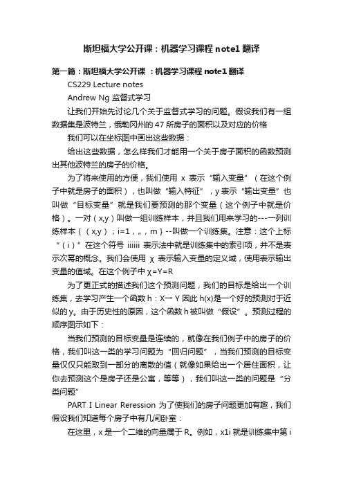
假设我们有一组数据集是波特兰,俄勒冈州的47所房子的面积以及对应的价格我们可以在坐标图中画出这些数据:给出这些数据,怎么样我们才能用一个关于房子面积的函数预测出其他波特兰的房子的价格。
为了将来使用的方便,我们使用x表示“输入变量”(在这个例子中就是房子的面积),也叫做“输入特征”,y表示“输出变量”也叫做“目标变量”就是我们要预测的那个变量(这个例子中就是价格)。
一对(x,y)叫做一组训练样本,并且我们用来学习的---一列训练样本{(x,y);i=1,…,m}--叫做一个训练集。
注意:这个上标“(i)”在这个符号iiiiii表示法中就是训练集中的索引项,并不是表示次幂的概念。
我们会使用χ表示输入变量的定义域,使用表示输出变量的值域。
在这个例子中χ=Y=R为了更正式的描述我们这个预测问题,我们的目标是给出一个训练集,去学习产生一个函数h:X→ Y 因此h(x)是一个好的预测对于近似的y。
由于历史性的原因,这个函数h被叫做“假设”。
预测过程的顺序图示如下:当我们预测的目标变量是连续的,就像在我们例子中的房子的价格,我们叫这一类的学习问题为“回归问题”,当我们预测的目标变量仅仅只能取到一部分的离散的值(就像如果给出一个居住面积,让你去预测这个是房子还是公寓,等等),我们叫这一类的问题是“分类问题”PART I Linear Reression 为了使我们的房子问题更加有趣,我们假设我们知道每个房子中有几间卧室:在这里,x是一个二维的向量属于R。
例如,x1i就是训练集中第i个房子的居住面积,i是训练集中第i个房子的卧室数量。
(通常情况下,当设计一个学习问题的时候,这些输x22入变量是由你决定去选择哪些,因此如果你是在Portland收集房子的数据,你可能会决定包含其他的特征,比如房子是否带有壁炉,这个洗澡间的数量等等。
机器学习 深度学习 笔记 (9)

minima or global minima of the cost function. Also note that the underlying
parameterization for hθ(x) is different from the case of linear regression, even though the form of the cost function is the same mean-squared loss.
θ := θ − α∇θJ (j)(θ)
(1.4)
Oftentimes computing the gradient of B examples simultaneously for the parameter θ can be faster than computing B gradients separately due to hardware parallelization. Therefore, a mini-batch version of SGD is most commonly used in deep learning, as shown in Algorithm 2. There are also other variants of the SGD or mini-batch SGD with slightly different sampling schemes.
3
Algorithm 2 Mini-batch Stochastic Gradient Descent
1: Hyperparameters: learning rate α, batch size B, # iterations niter. 2: Initialize θ randomly 3: for i = 1 to niter do 4: Sample B examples j1, . . . , jB (without replacement) uniformly from
EM笔记
维基百科说明:EM是一个在已知部分相关变量的情况下,估计未知变量的迭代技术。
EM的算法流程如下:初始化分布参数重复直到收敛:E步骤:估计未知参数的期望值,给出当前的参数估计。
M步骤:重新估计分布参数,以使得数据的似然性最大,给出未知变量的期望估计。
应用于缺失值。
最大期望过程说明我们用表示能够观察到的不完整的变量值,用表示无法观察到的变量值,这样和一起组成了完整的数据。
可能是实际测量丢失的数据,也可能是能够简化问题的隐藏变量,如果它的值能够知道的话。
例如,在混合模型(Mixture Model)中,如果“产生”样本的混合元素成分已知的话最大似然公式将变得更加便利(参见下面的例子)。
[编辑]估计无法观测的数据让代表矢量θ:定义的参数的全部数据的概率分布(连续情况下)或者概率聚类函数(离散情况下),那么从这个函数就可以得到全部数据的最大似然值,另外,在给定的观察到的数据条件下未知数据的条件分布可以表示为:百度百科:EM算法就是这样,假设我们估计知道A和B两个参数,在开始状态下二者都是未知的,并且知道了A的信息就可以得到B的信息,反过来知道了B也就得到了A。
可以考虑首先赋予A某种初值,以此得到B的估计值,然后从B的当前值出发,重新估计A的取值,这个过程一直持续到收敛为止。
EM 算法是Dempster,Laind,Rubin 于1977 年提出的求参数极大似然估计的一种方法,它可以从非完整数据集中对参数进行MLE 估计,是一种非常简单实用的学习算法。
这种方法可以广泛地应用于处理缺损数据,截尾数据,带有噪声等所谓的不完全数据(incomplete data)。
假定集合Z = (X,Y)由观测数据X 和未观测数据Y 组成,Z = (X,Y)和X 分别称为完整数据和不完整数据。
假设Z的联合概率密度被参数化地定义为P(X,Y|Θ),其中Θ 表示要被估计的参数。
Θ 的最大似然估计是求不完整数据的对数似然函数L(X;Θ)的最大值而得到的:L(Θ; X )= log p(X |Θ) = ∫log p(X ,Y |Θ)dY ;EM算法包括两个步骤:由E步和M步组成,它是通过迭代地最大化完整数据的对数似然函数Lc( X;Θ )的期望来最大化不完整数据的对数似然函数,其中:Lc(X;Θ) =log p(X,Y |Θ) ;假设在算法第t次迭代后Θ 获得的估计记为Θ(t ) ,则在(t+1)次迭代时,记为Θ(t +1).E-步:计算完整数据的对数似然函数的期望,记为:Q(Θ |Θ (t) ) = E{Lc(Θ;Z)|X;Θ(t) };M-步:通过最大化Q(Θ |Θ(t) ) 来获得新的Θ 。
斯坦福大学 CS229 机器学习notes12
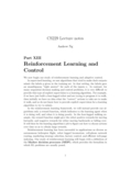
CS229Lecture notesAndrew NgPart XIIIReinforcement Learning and ControlWe now begin our study of reinforcement learning and adaptive control.In supervised learning,we saw algorithms that tried to make their outputs mimic the labels y given in the training set.In that setting,the labels gave an unambiguous“right answer”for each of the inputs x.In contrast,for many sequential decision making and control problems,it is very difficult to provide this type of explicit supervision to a learning algorithm.For example, if we have just built a four-legged robot and are trying to program it to walk, then initially we have no idea what the“correct”actions to take are to make it walk,and so do not know how to provide explicit supervision for a learning algorithm to try to mimic.In the reinforcement learning framework,we will instead provide our al-gorithms only a reward function,which indicates to the learning agent when it is doing well,and when it is doing poorly.In the four-legged walking ex-ample,the reward function might give the robot positive rewards for moving forwards,and negative rewards for either moving backwards or falling over. It will then be the learning algorithm’s job tofigure out how to choose actions over time so as to obtain large rewards.Reinforcement learning has been successful in applications as diverse as autonomous helicopterflight,robot legged locomotion,cell-phone network routing,marketing strategy selection,factory control,and efficient web-page indexing.Our study of reinforcement learning will begin with a definition of the Markov decision processes(MDP),which provides the formalism in which RL problems are usually posed.12 1Markov decision processesA Markov decision process is a tuple(S,A,{P sa},γ,R),where:•S is a set of states.(For example,in autonomous helicopterflight,S might be the set of all possible positions and orientations of the heli-copter.)•A is a set of actions.(For example,the set of all possible directions in which you can push the helicopter’s control sticks.)•P sa are the state transition probabilities.For each state s∈S and action a∈A,P sa is a distribution over the state space.We’ll say more about this later,but briefly,P sa gives the distribution over what states we will transition to if we take action a in state s.•γ∈[0,1)is called the discount factor.•R:S×A→R is the reward function.(Rewards are sometimes also written as a function of a state S only,in which case we would have R:S→R).The dynamics of an MDP proceeds as follows:We start in some state s0, and get to choose some action a0∈A to take in the MDP.As a result of our choice,the state of the MDP randomly transitions to some successor states1,drawn according to s1∼P s0a0.Then,we get to pick another action a1.As a result of this action,the state transitions again,now to some s2∼P s1a1.We then pick a2,and so on....Pictorially,we can represent this process as follows:s0a0−→s1a1−→s2a2−→s3a3−→...Upon visiting the sequence of states s0,s1,...with actions a0,a1,...,our total payoffis given byR(s0,a0)+γR(s1,a1)+γ2R(s2,a2)+···.Or,when we are writing rewards as a function of the states only,this becomesR(s0)+γR(s1)+γ2R(s2)+···.For most of our development,we will use the simpler state-rewards R(s), though the generalization to state-action rewards R(s,a)offers no special difficulties.3 Our goal in reinforcement learning is to choose actions over time so as to maximize the expected value of the total payoff:E R(s0)+γR(s1)+γ2R(s2)+···Note that the reward at timestep t is discounted by a factor ofγt.Thus,to make this expectation large,we would like to accrue positive rewards as soon as possible(and postpone negative rewards as long as possible).In economic applications where R(·)is the amount of money made,γalso has a natural interpretation in terms of the interest rate(where a dollar today is worth more than a dollar tomorrow).A policy is any functionπ:S→A mapping from the states to the actions.We say that we are executing some policyπif,whenever we are in state s,we take action a=π(s).We also define the value function for a policyπaccording toVπ(s)=E R(s0)+γR(s1)+γ2R(s2)+··· s0=s,π].Vπ(s)is simply the expected sum of discounted rewards upon starting in state s,and taking actions according toπ.1Given afixed policyπ,its value function Vπsatisfies the Bellman equa-tions:Vπ(s)=R(s)+γ s ∈S P sπ(s)(s )Vπ(s ).This says that the expected sum of discounted rewards Vπ(s)for starting in s consists of two terms:First,the immediate reward R(s)that we get rightaway simply for starting in state s,and second,the expected sum of future discounted rewards.Examining the second term in more detail,we[Vπ(s )].This see that the summation term above can be rewritten E s ∼Psπ(s)is the expected sum of discounted rewards for starting in state s ,where s is distributed according P sπ(s),which is the distribution over where we will end up after taking thefirst actionπ(s)in the MDP from state s.Thus,the second term above gives the expected sum of discounted rewards obtained after thefirst step in the MDP.Bellman’s equations can be used to efficiently solve for Vπ.Specifically, in afinite-state MDP(|S|<∞),we can write down one such equation for Vπ(s)for every state s.This gives us a set of|S|linear equations in|S| variables(the unknown Vπ(s)’s,one for each state),which can be efficiently solved for the Vπ(s)’s.1This notation in which we condition onπisn’t technically correct becauseπisn’t a random variable,but this is quite standard in the literature.4We also define the optimal value function according toV ∗(s )=max πV π(s ).(1)In other words,this is the best possible expected sum of discounted rewards that can be attained using any policy.There is also a version of Bellman’s equations for the optimal value function:V ∗(s )=R (s )+max a ∈A γ s ∈SP sa (s )V ∗(s ).(2)The first term above is the immediate reward as before.The second term is the maximum over all actions a of the expected future sum of discounted rewards we’ll get upon after action a .You should make sure you understand this equation and see why it makes sense.We also define a policy π∗:S →A as follows:π∗(s )=arg max a ∈A s ∈SP sa (s )V ∗(s ).(3)Note that π∗(s )gives the action a that attains the maximum in the “max”in Equation (2).It is a fact that for every state s and every policy π,we haveV ∗(s )=V π∗(s )≥V π(s ).The first equality says that the V π∗,the value function for π∗,is equal to the optimal value function V ∗for every state s .Further,the inequality above says that π∗’s value is at least a large as the value of any other other policy.In other words,π∗as defined in Equation (3)is the optimal policy.Note that π∗has the interesting property that it is the optimal policy for all states s .Specifically,it is not the case that if we were starting in some state s then there’d be some optimal policy for that state,and if we were starting in some other state s then there’d be some other policy that’s optimal policy for s .Specifically,the same policy π∗attains the maximum in Equation (1)for all states s .This means that we can use the same policy π∗no matter what the initial state of our MDP is.2Value iteration and policy iterationWe now describe two efficient algorithms for solving finite-state MDPs.For now,we will consider only MDPs with finite state and action spaces (|S |<∞,|A |<∞).The first algorithm,value iteration ,is as follows:51.For each state s,initialize V(s):=0.2.Repeat until convergence{For every state,update V(s):=R(s)+max a∈Aγ s P sa(s )V(s ).}This algorithm can be thought of as repeatedly trying to update the esti-mated value function using Bellman Equations(2).There are two possible ways of performing the updates in the inner loop of the algorithm.In thefirst,we canfirst compute the new values for V(s)for every state s,and then overwrite all the old values with the new values.This is called a synchronous update.In this case,the algorithm can be viewed as implementing a“Bellman backup operator”that takes a current estimate of the value function,and maps it to a new estimate.(See homework problem for details.)Alternatively,we can also perform asynchronous updates. Here,we would loop over the states(in some order),updating the values one at a time.Under either synchronous or asynchronous updates,it can be shown that value iteration will cause V to converge to V∗.Having found V∗,we can then use Equation(3)tofind the optimal policy.Apart from value iteration,there is a second standard algorithm forfind-ing an optimal policy for an MDP.The policy iteration algorithm proceeds as follows:1.Initializeπrandomly.2.Repeat until convergence{(a)Let V:=Vπ.(b)For each state s,letπ(s):=arg max a∈A s P sa(s )V(s ).}Thus,the inner-loop repeatedly computes the value function for the current policy,and then updates the policy using the current value function.(The policyπfound in step(b)is also called the policy that is greedy with re-spect to V.)Note that step(a)can be done via solving Bellman’s equations as described earlier,which in the case of afixed policy,is just a set of|S| linear equations in|S|variables.After at most afinite number of iterations of this algorithm,V will con-verge to V∗,andπwill converge toπ∗.6Both value iteration and policy iteration are standard algorithms for solv-ing MDPs,and there isn’t currently universal agreement over which algo-rithm is better.For small MDPs,policy iteration is often very fast and converges with very few iterations.However,for MDPs with large state spaces,solving for Vπexplicitly would involve solving a large system of lin-ear equations,and could be difficult.In these problems,value iteration may be preferred.For this reason,in practice value iteration seems to be used more often than policy iteration.3Learning a model for an MDPSo far,we have discussed MDPs and algorithms for MDPs assuming that the state transition probabilities and rewards are known.In many realistic prob-lems,we are not given state transition probabilities and rewards explicitly, but must instead estimate them from data.(Usually,S,A andγare known.) For example,suppose that,for the inverted pendulum problem(see prob-lem set4),we had a number of trials in the MDP,that proceeded as follows:s(1)0a (1) 0−→s(1)1a (1) 1−→s(1)2a (1) 2−→s(1)3a (1) 3−→...s(2)0a (2) 0−→s(2)1a (2) 1−→s(2)2a (2) 2−→s(2)3a (2) 3−→......Here,s(j)i is the state we were at time i of trial j,and a(j)i is the cor-responding action that was taken from that state.In practice,each of the trials above might be run until the MDP terminates(such as if the pole falls over in the inverted pendulum problem),or it might be run for some large butfinite number of timesteps.Given this“experience”in the MDP consisting of a number of trials, we can then easily derive the maximum likelihood estimates for the state transition probabilities:P sa(s )=#times took we action a in state s and got to s#times we took action a in state s(4)Or,if the ratio above is“0/0”—corresponding to the case of never having taken action a in state s before—the we might simply estimate P sa(s )to be 1/|S|.(I.e.,estimate P sa to be the uniform distribution over all states.) Note that,if we gain more experience(observe more trials)in the MDP, there is an efficient way to update our estimated state transition probabilities7 using the new experience.Specifically,if we keep around the counts for both the numerator and denominator terms of(4),then as we observe more trials, we can simply keep accumulating those puting the ratio of these counts then given our estimate of P sa.Using a similar procedure,if R is unknown,we can also pick our estimate of the expected immediate reward R(s)in state s to be the average reward observed in state s.Having learned a model for the MDP,we can then use either value it-eration or policy iteration to solve the MDP using the estimated transition probabilities and rewards.For example,putting together model learning and value iteration,here is one possible algorithm for learning in an MDP with unknown state transition probabilities:1.Initializeπrandomly.2.Repeat{(a)Executeπin the MDP for some number of trials.(b)Using the accumulated experience in the MDP,update our esti-mates for P sa(and R,if applicable).(c)Apply value iteration with the estimated state transition probabil-ities and rewards to get a new estimated value function V.(d)Updateπto be the greedy policy with respect to V.}We note that,for this particular algorithm,there is one simple optimiza-tion that can make it run much more quickly.Specifically,in the inner loop of the algorithm where we apply value iteration,if instead of initializing value iteration with V=0,we initialize it with the solution found during the pre-vious iteration of our algorithm,then that will provide value iteration with a much better initial starting point and make it converge more quickly.。
cs229斯坦福大学机器学习教程 Lecture note
CS 229 Machine LearningAndrew NgStanford UniversityContentsNote1:Supervised learning 1Note2:Generative Learning algorithms 31Note3:Support Vector Machines 45Note4:Learning Theory 70Note5:Regularization and model selection 81Note6:The perceptron and large margin classifiers 89 Note7a:The k-means clustering algorithm 92Note7b:Mixtures of Gaussians and the EM algorithm 95 Note8:The EM algorithm 99Note9:Factor analysis 107Note10:Principal components analysis 116Note11:Independent Components analysis 122Note12:Reinforcement Learning and Control 128CS229Lecture notesAndrew NgSupervised learningLets start by talking about a few examples of supervised learning problems.Suppose we have a dataset giving the living areas and prices of 47houses from Portland,Oregon:Living area (feet 2)Price (1000$s)21044001600330240036914162323000540......We can plot this data:Given data like this,how can we learn to predict the prices of other houses in Portland,as a function of the size of their living areas?1CS229Winter 20032To establish notation for future use,we’ll use x (i )to denote the “input”variables (living area in this example),also called input features ,and y (i )to denote the “output”or target variable that we are trying to predict (price).A pair (x (i ),y (i ))is called a training example ,and the dataset that we’ll be using to learn—a list of m training examples {(x (i ),y (i ));i =1,...,m }—is called a training set .Note that the superscript “(i )”in the notation is simply an index into the training set,and has nothing to do with exponentiation.We will also use X denote the space of input values,and Y the space of output values.In this example,X =Y =R .To describe the supervised learning problem slightly more formally,our goal is,given a training set,to learn a function h :X →Y so that h (x )is a “good”predictor for the corresponding value of y .For historical reasons,this function h is called a hypothesis .Seen pictorially,the process is therefore like this:house.)xof house)When the target variable that we’re trying to predict is continuous,such as in our housing example,we call the learning problem a regression prob-lem.When y can take on only a small number of discrete values (such as if,given the living area,we wanted to predict if a dwelling is a house or an apartment,say),we call it a classification problem.3Part ILinear RegressionTo make our housing example more interesting,lets consider a slightly richer dataset in which we also know the number of bedrooms in each house:Living area (feet 2)#bedrooms Price (1000$s)2104340016003330240033691416223230004540.........Here,the x ’s are two-dimensional vectors in R 2.For instance,x (i )1is theliving area of the i -th house in the training set,and x (i )2is its number ofbedrooms.(In general,when designing a learning problem,it will be up to you to decide what features to choose,so if you are out in Portland gathering housing data,you might also decide to include other features such as whether each house has a fireplace,the number of bathrooms,and so on.We’ll say more about feature selection later,but for now lets take the features as given.)To perform supervised learning,we must decide how we’re going to rep-resent functions/hypotheses h in a computer.As an initial choice,lets say we decide to approximate y as a linear function of x :h θ(x )=θ0+θ1x 1+θ2x 2Here,the θi ’s are the parameters (also called weights )parameterizing the space of linear functions mapping from X to Y .When there is no risk of confusion,we will drop the θsubscript in h θ(x ),and write it more simply as h (x ).To simplify our notation,we also introduce the convention of letting x 0=1(this is the intercept term ),so thath (x )=n i =0θi x i =θT x,where on the right-hand side above we are viewing θand x both as vectors,and here n is the number of input variables (not counting x 0).Now,given a training set,how do we pick,or learn,the parameters θ?One reasonable method seems to be to make h (x )close to y ,at least for4 the training examples we have.To formalize this,we will define a function that measures,for each value of theθ’s,how close the h(x(i))’s are to the corresponding y(i)’s.We define the cost function:J(θ)=12mi=1(hθ(x(i))−y(i))2.If you’ve seen linear regression before,you may recognize this as the familiar least-squares cost function that gives rise to the ordinary least squares regression model.Whether or not you have seen it previously,lets keep going,and we’ll eventually show this to be a special case of a much broader family of algorithms.1LMS algorithmWe want to chooseθso as to minimize J(θ).To do so,lets use a search algorithm that starts with some“initial guess”forθ,and that repeatedly changesθto make J(θ)smaller,until hopefully we converge to a value of θthat minimizes J(θ).Specifically,lets consider the gradient descent algorithm,which starts with some initialθ,and repeatedly performs the update:θj:=θj−α∂∂θjJ(θ).(This update is simultaneously performed for all values of j=0,...,n.) Here,αis called the learning rate.This is a very natural algorithm that repeatedly takes a step in the direction of steepest decrease of J.In order to implement this algorithm,we have to work out what is the partial derivative term on the right hand side.Letsfirst work it out for the case of if we have only one training example(x,y),so that we can neglect the sum in the definition of J.We have:∂∂θj J(θ)=∂∂θj12(hθ(x)−y)2=2·12(hθ(x)−y)·∂∂θj(hθ(x)−y) =(hθ(x)−y)·∂∂θj n i=0θi x i−y=(hθ(x)−y)x j5 For a single training example,this gives the update rule:1θj:=θj+α y(i)−hθ(x(i)) x(i)j.The rule is called the LMS update rule(LMS stands for“least mean squares”), and is also known as the Widrow-Hofflearning rule.This rule has several properties that seem natural and intuitive.For instance,the magnitude of the update is proportional to the error term(y(i)−hθ(x(i)));thus,for in-stance,if we are encountering a training example on which our prediction nearly matches the actual value of y(i),then wefind that there is little need to change the parameters;in contrast,a larger change to the parameters will be made if our prediction hθ(x(i))has a large error(i.e.,if it is very far from y(i)).We’d derived the LMS rule for when there was only a single training example.There are two ways to modify this method for a training set of more than one example.Thefirst is replace it with the following algorithm: Repeat until convergence{θj:=θj+α m i=1 y(i)−hθ(x(i)) x(i)j(for every j).}The reader can easily verify that the quantity in the summation in the update rule above is just∂J(θ)/∂θj(for the original definition of J).So,this is simply gradient descent on the original cost function J.This method looks at every example in the entire training set on every step,and is called batch gradient descent.Note that,while gradient descent can be susceptible to local minima in general,the optimization problem we have posed here for linear regression has only one global,and no other local,optima;thus gradient descent always converges(assuming the learning rateαis not too large)to the global minimum.Indeed,J is a convex quadratic function. Here is an example of gradient descent as it is run to minimize a quadratic function.1We use the notation“a:=b”to denote an operation(in a computer program)in which we set the value of a variable a to be equal to the value of b.In other words,this operation overwrites a with the value of b.In contrast,we will write“a=b”when we are asserting a statement of fact,that the value of a is equal to the value of b.6The Also shown is the trajectory taken by gradient descent,with was initialized at (48,30).The x’s in thefigure(joined by straight lines)mark the successive values ofθthat gradient descent went through.When we run batch gradient descent tofitθon our previous dataset, to learn to predict housing price as a function of living area,we obtain θ0=71.27,θ1=0.1345.If we plot hθ(x)as a function of x(area),along with the training data,we obtain the followingfigure:If the number of bedrooms were included as one of the input features as well, we getθ0=89.60,θ1=0.1392,θ2=−8.738.The above results were obtained with batch gradient descent.There is an alternative to batch gradient descent that also works very well.Consider the following algorithm:7Loop{for i=1to m,{θj:=θj+α y(i)−hθ(x(i)) x(i)j(for every j).}}In this algorithm,we repeatedly run through the training set,and each time we encounter a training example,we update the parameters according to the gradient of the error with respect to that single training example only. This algorithm is called stochastic gradient descent(also incremental gradient descent).Whereas batch gradient descent has to scan through the entire training set before taking a single step—a costly operation if m is large—stochastic gradient descent can start making progress right away,and continues to make progress with each example it looks at.Often,stochastic gradient descent getsθ“close”to the minimum much faster than batch gra-dient descent.(Note however that it may never“converge”to the minimum, and the parametersθwill keep oscillating around the minimum of J(θ);but in practice most of the values near the minimum will be reasonably good approximations to the true minimum.2)For these reasons,particularly when the training set is large,stochastic gradient descent is often preferred over batch gradient descent.2The normal equationsGradient descent gives one way of minimizing J.Lets discuss a second way of doing so,this time performing the minimization explicitly and without resorting to an iterative algorithm.In this method,we will minimize J by explicitly taking its derivatives with respect to theθj’s,and setting them to zero.To enable us to do this without having to write reams of algebra and pages full of matrices of derivatives,lets introduce some notation for doing calculus with matrices.2While it is more common to run stochastic gradient descent as we have described it and with afixed learning rateα,by slowly letting the learning rateαdecrease to zero as the algorithm runs,it is also possible to ensure that the parameters will converge to the global minimum rather then merely oscillate around the minimum.82.1Matrix derivativesFor a function f :R m ×n →R mapping from m -by-n matrices to the real numbers,we define the derivative of f with respect to A to be:∇A f (A )= ∂f ∂A 11···∂f ∂A 1n .........∂f ∂A m 1···∂f ∂A mnThus,the gradient ∇A f (A )is itself an m -by-n matrix,whose (i,j )-element is ∂f/∂A ij .For example,suppose A = A 11A 12A 21A 22 is a 2-by-2matrix,and the function f :R 2×2→R is given byf (A )=32A 11+5A 212+A 21A 22.Here,A ij denotes the (i,j )entry of the matrix A .We then have ∇A f (A )= 3210A 12A 22A 21 .We also introduce the trace operator,written “tr.”For an n -by-n (square)matrix A ,the trace of A is defined to be the sum of its diagonal entries:tr A =n i =1A iiIf a is a real number (i.e.,a 1-by-1matrix),then tr a =a .(If you haven’t seen this “operator notation”before,you should think of the trace of A as tr(A ),or as application of the “trace”function to the matrix A .It’s more commonly written without the parentheses,however.)The trace operator has the property that for two matrices A and B such that AB is square,we have that tr AB =tr BA .(Check this yourself!)As corollaries of this,we also have,e.g.,tr ABC =tr CAB =tr BCA,tr ABCD =tr DABC =tr CDAB =tr BCDA.The following properties of the trace operator are also easily verified.Here,A and B are square matrices,and a is a real number:tr A =tr A Ttr(A +B )=tr A +tr Btr aA =a tr A9 We now state without proof some facts of matrix derivatives(we won’t need some of these until later this quarter).Equation(4)applies only to non-singular square matrices A,where|A|denotes the determinant of A.We have:∇A tr AB=B T(1)∇A T f(A)=(∇A f(A))T(2)∇A tr ABA T C=CAB+C T AB T(3)∇A|A|=|A|(A−1)T.(4) To make our matrix notation more concrete,let us now explain in detail the meaning of thefirst of these equations.Suppose we have somefixed matrix B∈R n×m.We can then define a function f:R m×n→R according to f(A)=tr AB.Note that this definition makes sense,because if A∈R m×n, then AB is a square matrix,and we can apply the trace operator to it;thus, f does indeed map from R m×n to R.We can then apply our definition of matrix derivatives tofind∇A f(A),which will itself by an m-by-n matrix. Equation(1)above states that the(i,j)entry of this matrix will be given by the(i,j)-entry of B T,or equivalently,by B ji.The proofs of Equations(1-3)are reasonably simple,and are left as an exercise to the reader.Equations(4)can be derived using the adjoint repre-sentation of the inverse of a matrix.32.2Least squares revisitedArmed with the tools of matrix derivatives,let us now proceed tofind in closed-form the value ofθthat minimizes J(θ).We begin by re-writing J in matrix-vectorial notation.Giving a training set,define the design matrix X to be the m-by-n matrix(actually m-by-n+1,if we include the intercept term)that contains 3If we define A′to be the matrix whose(i,j)element is(−1)i+j times the determinant of the square matrix resulting from deleting row i and column j from A,then it can be proved that A−1=(A′)T/|A|.(You can check that this is consistent with the standard way offinding A−1when A is a2-by-2matrix.If you want to see a proof of this more general result,see an intermediate or advanced linear algebra text,such as Charles Curtis, 1991,Linear Algebra,Springer.)This shows that A′=|A|(A−1)T.Also,the determinant of a matrix can be written|A|= j A ij A′ij.Since(A′)ij does not depend on A ij(as can be seen from its definition),this implies that(∂/∂A ij)|A|=A′ij.Putting all this together shows the result.10the training examples’input values in its rows:X = —(x (1))T ——(x (2))T —...—(x (m ))T —.Also,let y be the m -dimensional vector containing all the target values from the training set: y = y (1)y (2)...y (m ) .Now,since h θ(x (i ))=(x (i ))T θ,we can easily verifythat Xθ− y = (x (1))T θ...(x (m ))T θ − y (1)...y (m ) = h θ(x (1))−y (1)...h θ(x (m ))−y (m ) .Thus,using the fact that for a vector z ,we have that z T z =i z 2i :12(Xθ− y )T (Xθ− y )=12m i =1(h θ(x (i ))−y (i ))2=J (θ)Finally,to minimize J ,lets find its derivatives with respect to θ.Combining Equations (2)and (3),we find that∇A T tr ABA T C =B T A T C T +BA T C (5)11Hence,∇θJ (θ)=∇θ12(Xθ− y )T (Xθ− y )=12∇θ θT X T Xθ−θT X T y − y T Xθ+ y T y =12∇θtr θT X T Xθ−θT X T y − y T Xθ+ y T y =12∇θ tr θT X T Xθ−2tr y T Xθ =12X T Xθ+X T Xθ−2X T y =X T Xθ−X T yIn the third step,we used the fact that the trace of a real number is just the real number;the fourth step used the fact that tr A =tr A T ,and the fifth step used Equation (5)with A T =θ,B =B T =X T X ,and C =I ,and Equation (1).To minimize J ,we set its derivatives to zero,and obtain the normal equations :X T Xθ=X T yThus,the value of θthat minimizes J (θ)is given in closed form by the equationθ=(X T X )−1X T y .3Probabilistic interpretationWhen faced with a regression problem,why might linear regression,and specifically why might the least-squares cost function J ,be a reasonable choice?In this section,we will give a set of probabilistic assumptions,under which least-squares regression is derived as a very natural algorithm.Let us assume that the target variables and the inputs are related via the equationy (i )=θT x (i )+ǫ(i ),where ǫ(i )is an error term that captures either unmodeled effects (such as if there are some features very pertinent to predicting housing price,but that we’d left out of the regression),or random noise.Let us further assume that the ǫ(i )are distributed IID (independently and identically distributed)according to a Gaussian distribution (also called a Normal distribution)with12 mean zero and some varianceσ2.We can write this assumption as“ǫ(i)∼N(0,σ2).”I.e.,the density ofǫ(i)is given byp(ǫ(i))=1√2πσexp −(ǫ(i))22σ2 .This implies thatp(y(i)|x(i);θ)=1√2πσexp −(y(i)−θT x(i))22σ2 .The notation“p(y(i)|x(i);θ)”indicates that this is the distribution of y(i) given x(i)and parameterized byθ.Note that we should not condition onθ(“p(y(i)|x(i),θ)”),sinceθis not a random variable.We can also write the distribution of y(i)as as y(i)|x(i);θ∼N(θT x(i),σ2).Given X(the design matrix,which contains all the x(i)’s)andθ,what is the distribution of the y(i)’s?The probability of the data is given by p( y|X;θ).This quantity is typically viewed a function of y(and perhaps X), for afixed value ofθ.When we wish to explicitly view this as a function of θ,we will instead call it the likelihood function:L(θ)=L(θ;X, y)=p( y|X;θ).Note that by the independence assumption on theǫ(i)’s(and hence also the y(i)’s given the x(i)’s),this can also be writtenL(θ)=mi=1p(y(i)|x(i);θ)=mi=11√2πσexp −(y(i)−θT x(i))22σ2 .Now,given this probabilistic model relating the y(i)’s and the x(i)’s,what is a reasonable way of choosing our best guess of the parametersθ?The principal of maximum likelihood says that we should should chooseθso as to make the data as high probability as possible.I.e.,we should chooseθto maximize L(θ).Instead of maximizing L(θ),we can also maximize any strictly increasing function of L(θ).In particular,the derivations will be a bit simpler if we13 instead maximize the log likelihoodℓ(θ):ℓ(θ)=log L(θ)=logmi=11√2πσexp −(y(i)−θT x(i))22σ2=mi=1log1√2πσexp −(y(i)−θT x(i))22σ2=m log1√2πσ−1σ2·12mi=1(y(i)−θT x(i))2.Hence,maximizingℓ(θ)gives the same answer as minimizing1 2mi=1(y(i)−θT x(i))2,which we recognize to be J(θ),our original least-squares cost function.To summarize:Under the previous probabilistic assumptions on the data, least-squares regression corresponds tofinding the maximum likelihood esti-mate ofθ.This is thus one set of assumptions under which least-squares re-gression can be justified as a very natural method that’s just doing maximum likelihood estimation.(Note however that the probabilistic assumptions are by no means necessary for least-squares to be a perfectly good and rational procedure,and there may—and indeed there are—other natural assumptions that can also be used to justify it.)Note also that,in our previous discussion,ourfinal choice ofθdid not depend on what wasσ2,and indeed we’d have arrived at the same result even ifσ2were unknown.We will use this fact again later,when we talk about the exponential family and generalized linear models.4Locally weighted linear regressionConsider the problem of predicting y from x∈R.The leftmostfigure below shows the result offitting a y=θ0+θ1x to a dataset.We see that the data doesn’t really lie on straight line,and so thefit is not very good.14Instead,if we had added an extra feature x2,andfit y=θ0+θ1x+θ2x2,then we obtain a slightly betterfit to the data.(See middlefigure)Naively,itmight seem that the more features we add,the better.However,there is alsoa danger in adding too many features:The rightmostfigure is the result offitting a5-th order polynomial y= 5j=0θj x j.We see that even though the fitted curve passes through the data perfectly,we would not expect this tobe a very good predictor of,say,housing prices(y)for different living areas(x).Without formally defining what these terms mean,we’ll say thefigureon the left shows an instance of underfitting—in which the data clearlyshows structure not captured by the model—and thefigure on the right isan example of overfitting.(Later in this class,when we talk about learningtheory we’ll formalize some of these notions,and also define more carefullyjust what it means for a hypothesis to be good or bad.)As discussed previously,and as shown in the example above,the choice offeatures is important to ensuring good performance of a learning algorithm.(When we talk about model selection,we’ll also see algorithms for automat-ically choosing a good set of features.)In this section,let us talk briefly talkabout the locally weighted linear regression(LWR)algorithm which,assum-ing there is sufficient training data,makes the choice of features less critical.This treatment will be brief,since you’ll get a chance to explore some of theproperties of the LWR algorithm yourself in the homework.In the original linear regression algorithm,to make a prediction at a querypoint x(i.e.,to evaluate h(x)),we would:1.Fitθto minimize i(y(i)−θT x(i))2.2.OutputθT x.In contrast,the locally weighted linear regression algorithm does the fol-lowing:1.Fitθto minimize i w(i)(y(i)−θT x(i))2.2.OutputθT x.15 Here,the w(i)’s are non-negative valued weights.Intuitively,if w(i)is large for a particular value of i,then in pickingθ,we’ll try hard to make(y(i)−θT x(i))2small.If w(i)is small,then the(y(i)−θT x(i))2error term will be pretty much ignored in thefit.A fairly standard choice for the weights is4w(i)=exp −(x(i)−x)22τ2Note that the weights depend on the particular point x at which we’re trying to evaluate x.Moreover,if|x(i)−x|is small,then w(i)is close to1;and if|x(i)−x|is large,then w(i)is small.Hence,θis chosen giving a much higher“weight”to the(errors on)training examples close to the query point x.(Note also that while the formula for the weights takes a form that is cosmetically similar to the density of a Gaussian distribution,the w(i)’s do not directly have anything to do with Gaussians,and in particular the w(i) are not random variables,normally distributed or otherwise.)The parameter τcontrols how quickly the weight of a training example falls offwith distance of its x(i)from the query point x;τis called the bandwidth parameter,and is also something that you’ll get to experiment with in your homework.Locally weighted linear regression is thefirst example we’re seeing of a non-parametric algorithm.The(unweighted)linear regression algorithm that we saw earlier is known as a parametric learning algorithm,because it has afixed,finite number of parameters(theθi’s),which arefit to the data.Once we’vefit theθi’s and stored them away,we no longer need to keep the training data around to make future predictions.In contrast,to make predictions using locally weighted linear regression,we need to keep the entire training set around.The term“non-parametric”(roughly)refers to the fact that the amount of stuffwe need to keep in order to represent the hypothesis h grows linearly with the size of the training set.4If x is vector-valued,this is generalized to be w(i)=exp(−(x(i)−x)T(x(i)−x)/(2τ2)), or w(i)=exp(−(x(i)−x)TΣ−1(x(i)−x)/2),for an appropriate choice ofτorΣ.16Part IIClassification and logistic regressionLets now talk about the classification problem.This is just like the regression problem,except that the values y we now want to predict take on only a small number of discrete values.For now,we will focus on the binary classification problem in which y can take on only two values,0and1. (Most of what we say here will also generalize to the multiple-class case.) For instance,if we are trying to build a spam classifier for email,then x(i) may be some features of a piece of email,and y may be1if it is a piece of spam mail,and0otherwise.0is also called the negative class,and1 the positive class,and they are sometimes also denoted by the symbols“-”and“+.”Given x(i),the corresponding y(i)is also called the label for the training example.5Logistic regressionWe could approach the classification problem ignoring the fact that y is discrete-valued,and use our old linear regression algorithm to try to predict y given x.However,it is easy to construct examples where this method performs very poorly.Intuitively,it also doesn’t make sense for hθ(x)to take values larger than1or smaller than0when we know that y∈{0,1}.Tofix this,lets change the form for our hypotheses hθ(x).We will choosehθ(x)=g(θT x)=11+e−θT x,whereg(z)=11+e−zis called the logistic function or the sigmoid function.Here is a plot showing g(z):17Notice that g(z)tends towards1as z→∞,and g(z)tends towards0as z→−∞.Moreover,g(z),and hence also h(x),is always bounded between 0and1.As before,we are keeping the convention of letting x0=1,so that θT x=θ0+ n j=1θj x j.For now,lets take the choice of g as given.Other functions that smoothly increase from0to1can also be used,but for a couple of reasons that we’ll see later(when we talk about GLMs,and when we talk about generative learning algorithms),the choice of the logistic function is a fairly natural one.Before moving on,here’s a useful property of the derivative of the sigmoid function, which we write a g′:g′(z)=ddz11+e−z=1 (1+e−z)2 e−z=1(1+e−z)·1−1(1+e−z)=g(z)(1−g(z)).So,given the logistic regression model,how do wefitθfor it?Follow-ing how we saw least squares regression could be derived as the maximum likelihood estimator under a set of assumptions,lets endow our classification model with a set of probabilistic assumptions,and thenfit the parameters via maximum likelihood.18 Let us assume thatP(y=1|x;θ)=hθ(x)P(y=0|x;θ)=1−hθ(x)Note that this can be written more compactly asp(y|x;θ)=(hθ(x))y(1−hθ(x))1−yAssuming that the m training examples were generated independently,we can then write down the likelihood of the parameters asL(θ)=p( y|X;θ)=mi=1p(y(i)|x(i);θ)=mi=1 hθ(x(i)) y(i) 1−hθ(x(i)) 1−y(i)As before,it will be easier to maximize the log likelihood:ℓ(θ)=log L(θ)=mi=1y(i)log h(x(i))+(1−y(i))log(1−h(x(i)))How do we maximize the likelihood?Similar to our derivation in the case of linear regression,we can use gradient ascent.Written in vectorial notation, our updates will therefore be given byθ:=θ+α∇θℓ(θ).(Note the positive rather than negative sign in the update formula,since we’re maximizing, rather than minimizing,a function now.)Lets start by working with just one training example(x,y),and take derivatives to derive the stochastic gradient ascent rule:∂∂θjℓ(θ)= y1g(θT x)−(1−y)11−g(θT x) ∂∂θj g(θT x)= y1g(θT x)−(1−y)11−g(θT x) g(θT x)(1−g(θT x)∂∂θjθT x= y(1−g(θT x))−(1−y)g(θT x) x j=(y−hθ(x))x j19Above,we used the fact that g′(z)=g(z)(1−g(z)).This therefore gives us the stochastic gradient ascent ruleθj:=θj+α y(i)−hθ(x(i)) x(i)jIf we compare this to the LMS update rule,we see that it looks identical;but this is not the same algorithm,because hθ(x(i))is now defined as a non-linear function ofθT x(i).Nonetheless,it’s a little surprising that we end up with the same update rule for a rather different algorithm and learning problem. Is this coincidence,or is there a deeper reason behind this?We’ll answer this when get get to GLM models.(See also the extra credit problem on Q3of problem set1.)6Digression:The perceptron learning algo-rithmWe now digress to talk briefly about an algorithm that’s of some historical interest,and that we will also return to later when we talk about learning theory.Consider modifying the logistic regression method to“force”it to output values that are either0or1or exactly.To do so,it seems natural to change the definition of g to be the threshold function:g(z)= 1if z≥00if z<0If we then let hθ(x)=g(θT x)as before but using this modified definition of g,and if we use the update ruleθj:=θj+α y(i)−hθ(x(i)) x(i)j.then we have the perceptron learning algorithm.In the1960s,this“perceptron”was argued to be a rough model for how individual neurons in the brain work.Given how simple the algorithm is,it will also provide a starting point for our analysis when we talk about learning theory later in this class.Note however that even though the perceptron may be cosmetically similar to the other algorithms we talked about,it is actually a very different type of algorithm than logistic regression and least squares linear regression;in particular,it is difficult to endow the perceptron’s predic-tions with meaningful probabilistic interpretations,or derive the perceptron as a maximum likelihood estimation algorithm.。
机器学习读书笔记

机器学习的基本概念和学习系统的设计
最近在看机器学习的书和视频,我的感觉是机器学习是很用的东西,而且是很多 学科交叉形成的领域。最相关的几个领域要属人工智能、概率统计、计算复tchell 第一章中和斯坦福机器学习公开课第一课都提到了 一个这样定义: 对于某类任务 T 和性能度量 P,如果一个计算机程序在 T 上以 P 衡量的性能随
概念学习
给定一样例集合以及每个样例是否属于某一概念的标注,怎样自动推断出该概念 的一般定义。这一问题被称为概念学习。 一个更准确的定义: 概念学习是指从有关某个布尔函数的输入输出训练样例中推断出该布尔函数。注 意,在前面一篇文章《机器学习的基本概念和学习系统的设计》中提到,机器学 习中要学习的知识的确切类型通常是一个函数,在概念学习里面,这个函数被限 定为是一个布尔函数,也就是它的输出只有{0,1}(0代表 false,1(代表 true)), 也就是说目标函数的形式如下:
x1:棋盘上黑子的数量
x2:棋盘上白子的数量
x3:棋盘上黑王的数量 x4:棋盘上红王的数量 x5:被红字威胁的黑子数量(即会在下一次被红子吃掉的黑子数量) x6:被黑子威胁的红子的数量 于是学习程序把 V’(b)表示为一个线性函数 V’(b)=w0 + w1x1 + w2x2 + w3x3 + w4x4 + w5x5 + w6x6 其中,w0到 w6为数字系数,或叫权,由学习算法来选择。在决定某一个棋盘状 态值,权 w1到 w6决定了不同的棋盘特征的相对重要性,而权 w0为一个附加的 棋盘状态值常量。 好了,现在我们把学习西洋跳棋战略的问题转化为学习目标函数表示中系数 w0 到 w6值的问题,也即选择函数逼近算法。 选择函数逼近算法 为了学习 V’(b),我们需要一系列训练样例,它的形式为<b, Vtrain(b)>其中,b 是由 x1-x6参数描述的棋盘状态,Vtrain(b)是 b 的训练值。 举例来说, <<x1=3,x2=0,x3=1,x4=0,x5=0,x6=0>, +100>;描述了一个黑棋取胜的棋盘 状态 b,因为 x2=0表示红旗已经没有子了。 上面的训练样例表示仍然有一个问题:虽然对弈结束时最终状态的棋盘的评分 Vtrain(b)很好确定,但是大量中间状态(未分出胜负)的棋盘如何评分呢? 于是这里需要一个训练值估计法则: Vtrain(b) <- V’(Successor(b)) Successor(b)表示 b 之后再轮到程序走棋时的棋盘状态(也就是程序走了一步 和对手回应了一步以后的棋局)。 这个看起来有点难理解,我们用当前的 V’来估计训练值,又用这一训练值来更 新 V’。当然,我们使用后续棋局 Successor(b)的估计值来估计棋局 b 的值。直
机器学习斯坦福课后作业笔记
作业三题目解析:本作业主要有两个知识点:使用逻辑回归来实现多分类问题(one-vs-all)以及神经网络应用,应用场景是机器学习辨认手写数字0到9。
多分类逻辑回归问题对于N分类问题(N>=3),就需要N个假设函数(预测模型),也即需要N组模型参数θ(θ一般是一个向量)然后,对于每个样本实例,依次使用每个模型预测输出,选取输出值最大的那组模型所对应的预测结果作为最终结果。
主要应用三个函数:predictOneVsAll.m, oneVsAll.m, lrCostFunction.m 其中,oneVsAll中用优化函数fmincg来找到最优参数,结果是参数矩阵k*n+1,其中k是多分类的类别数,n则是特征数,此处包含了k个模型,每个模型有各自的参数,在预测函数中,[c,i] = max(sigmoid(X * all_theta'), [], 2),把k个模型中结果最大的那个类别选中。
c是每一行中最大的数,是一个列向量,i是每一行最大的那个数字的列位置此处的主要是要求用向量规则计算损失函数和损失函数的倒数公式,不再利用循环。
损失函数(未应用正则化)如下:F:\mechine learning\ex3梯度函数如下在应用了正则化之后的函数如下,需要注意的是此时偏置参数不可计算在内,需要减去θ0梯度函数同理,θ0的求导要单独分开Matlab的max用法知识点加一:[a,b]=max(A, [], 2)函数中,a是每一行中最大的数,是一个列向量,b是每一行最大的那个数字的列位置神经网络的计算模型应用的具体语句,主要问题在于函数维数的准确把握,每一层都需要对输入进行一次添加偏置项,X是这样,a_super_2也是这样!作业四题目解析:首先用题目提供的参数在前向传播算法下实现多分类问题,其次需要用后向传播算法(BP神经网络)学习最优参数。
前向传播算法的计算主要完成的函数包括损失函数的编写。
其中,需要注意的是Θ(1) (Theta1)是一个25*401矩阵,行的数目为25,由隐藏层的单元个数决定(不包括bias unit),列的数目由输入特征数目决定(加上bias unit之后变成401)。
斯坦福大学机器学习课程个人笔记完整版.
CS 229机器学习(个人笔记目录 (1线性回归、logistic 回归和一般回归 1 (2判别模型、生成模型与朴素贝叶斯方法 10 (3支持向量机SVM (上) 20(4支持向量机SVM (下) 32(5规则化和模型选择 45(6K-means聚类算法 50(7混合高斯模型和EM 算法 53(8EM算法 55(9在线学习 62(10主成分分析 65(11独立成分分析 80(12线性判别分析 91(13因子分析 103(14增强学习 114(15典型关联分析 120(16偏最小二乘法回归 129这里面的内容是我在2011年上半年学习斯坦福大学《机器学习》课程的个人学习笔记,内容主要来自Andrew Ng教授的讲义和学习视频。
另外也包含来自其他论文和其他学校讲义的一些内容。
每章内容主要按照个人学习时的思路总结得到。
由于是个人笔记,里面表述错误、公式错误、理解错误、笔误都会存在。
更重要的是我是初学者,千万不要认为里面的思路都正确。
如果有疑问的地方,请第一时间参考Andrew Ng教授的讲义原文和视频,再有疑问的地方可以找一些大牛问问。
博客上很多网友提出的问题,我难以回答,因为我水平确实有限,更深层次的内容最好找相关大牛咨询和相关论文研读。
如果有网友想在我这个版本基础上再添加自己的笔记,可以发送 Email 给我,我提供原始的word docx版本。
另,本人目前在科苑软件所读研,马上三年了,方向是分布式计算,主要偏大数据分布式处理,平时主要玩Hadoop 、Pig 、Hive 、 Mahout 、NoSQL 啥的,关注系统方面和数据库方面的会议。
希望大家多多交流,以后会往博客上放这些内容,机器学习会放的少了。
Anyway ,祝大家学习进步、事业成功!1 对回归方法的认识JerryLead2011 年 2 月 27 日1 摘要本报告是在学习斯坦福大学机器学习课程前四节加上配套的讲义后的总结与认识。
前四节主要讲述了回归问题,属于有监督学习中的一种方法。
机器学习个人笔记完整版v4.21

机器学习个人笔记完整版v4.21摘要本笔记是针对斯坦福大学2014年机器学习课程视频做的个人笔记黄海广haiguang2000@qq:10822884斯坦福大学机器学习教程中文笔记课程概述Machine Learning(机器学习)是研究计算机怎样模拟或实现人类的学习行为,以获取新的知识或技能,重新组织已有的知识结构使之不断改善自身的性能。
它是人工智能的核心,是使计算机具有智能的根本途径,其应用遍及人工智能的各个领域,它主要使用归纳、综合而不是演译。
在过去的十年中,机器学习帮助我们自动驾驶汽车,有效的语音识别,有效的网络搜索,并极大地提高了人类基因组的认识。
机器学习是当今非常普遍,你可能会使用这一天几十倍而不自知。
很多研究者也认为这是最好的人工智能的取得方式。
在本课中,您将学习最有效的机器学习技术,并获得实践,让它们为自己的工作。
更重要的是,你会不仅得到理论基础的学习,而且获得那些需要快速和强大的应用技术解决问题的实用技术。
最后,你会学到一些硅谷利用机器学习和人工智能的最佳实践创新。
本课程提供了一个广泛的介绍机器学习、数据挖掘、统计模式识别的课程。
主题包括:(一)监督学习(参数/非参数算法,支持向量机,核函数,神经网络)。
(二)无监督学习(聚类,降维,推荐系统,深入学习推荐)。
(三)在机器学习的最佳实践(偏差/方差理论;在机器学习和人工智能创新过程)。
本课程还将使用大量的案例研究,您还将学习如何运用学习算法构建智能机器人(感知,控制),文本的理解(Web搜索,反垃圾邮件),计算机视觉,医疗信息,音频,数据挖掘,和其他领域。
本课程需要10周共18节课,相对以前的机器学习视频,这个视频更加清晰,而且每课都有ppt课件,推荐学习。
本人是中国海洋大学2014级博士生,目前刚开始接触机器学习,我下载了这次课程的所有视频和课件给大家分享。
中英文字幕来自于https:///course/ml,主要是教育无边界字幕组翻译,本人把中英文字幕进行合并,并翻译了部分字幕,对视频进行封装,归类,并翻译了课程目录,做好课程索引文件,希望对大家有所帮助。
机器学习笔记

机器学习笔记机器学习笔记总结预习部分第⼀章第⼀章主要讲述了机器学习与模式识别的概念,模型的概念和组成、特征向量的⼀些计算机器学习的基本概念机器学习可以分为监督式学习,⽆监督式学习,半监督式学习,强化学习。
以及模型的泛化能⼒,模型训练过程中存在的问题,如1、训练样本稀疏:给定的训练样本数量是有限的,很难完整表达样本的真实分布2、训练样本采样过程可能不均匀:有些区域采样密⼀些,有些区域采样疏⼀些3、⼀些样本可能带有噪声还有过拟合的概念模型训练阶段表现很好,但是在测试阶段表现差模型过于拟合训练如何提⾼泛化能⼒1、选择复杂度适合的模型:模型选择2、正则化:在⽬标函数中加⼊正则项评估⽅法与性能指标有留出法、交叉验证法、留⼀法性能度量⼆分类问题常⽤的评价指标时查准率和查全率。
根据预测正确与否,将样例分为以下四种:1)True positive(TP): 真正例,将正类正确预测为正类数;2)False positive(FP): 假正例,将负类错误预测为正类数;3)False negative(FN):假负例,将正类错误预测为负类数;4)True negative(TN): 真负例,将负类正确预测为负类数。
第⼆章第⼆章主要讲的是基于距离的分类器基于距离的分类的基本概念把样本到每个类的距离作为决策模型,将测式样本判定为与其距离最近的类常见的⼏种距离度量欧⽒距离(Euclidean Distance)曼哈顿距离(Manhattan Distance)加权欧式距离MED分类器最⼩欧⽒距离分类器距离衡量:欧⽒距离类的原型:均值特征⽩化⽬的:将原始特征映射到新的⼀个特征空间,使得在新空间中特征的协⽅差为单位矩阵,从⽽去除特征变化的不同及特征之间的相关性将特征转化分为两步:先去除特征之间的相关性(解耦),然后再对特征进⾏尺度变化(⽩化)马⽒距离马⽒距离表⽰数据的协⽅差距离。
它是⼀种有效的计算两个未知样本集的相似度的⽅法。
DeepLearning(深度学习)学习笔记整理系列

DeepLearning(深度学习)学习笔记整理系列Deep Learning(深度学习)学习笔记整理系列声明:1)该Deep Learning的学习系列是整理自网上很大牛和机器学习专家所无私奉献的资料的。
具体引用的资料请看参考文献。
具体的版本声明也参考原文献。
2)本文仅供学术交流,非商用。
所以每一部分具体的参考资料并没有详细对应。
如果某部分不小心侵犯了大家的利益,还望海涵,并联系博主删除。
3)本人才疏学浅,整理总结的时候难免出错,还望各位前辈不吝指正,谢谢。
4)阅读本文需要机器学习、计算机视觉、神经网络等等基础(如果没有也没关系了,没有就看看,能不能看懂,呵呵)。
5)此属于第一版本,若有错误,还供学术交流,非商用。
所以每一部分具体的参考资料并没有详细对应。
如果某部分不小心侵犯了大家的利益,还望海涵,并联系博主删除。
需继续修正与增删。
还望大家多多指点。
大家都共享一点点,一起为祖国科研的推进添砖加瓦(呵呵,好高尚的目标啊)。
请联系:zouxy09@/doc/8b6e8c3a5fbfc77da369b1 7b.html一、概述Artificial Intelligence,也就是人工智能,就像长生不老和星际漫游一样,是人类最美好的梦想之一。
虽然计算机技术已经取得了长足的进步,但是到目前为止,还没有一台电脑能产生―自我‖的意识。
是的,在人类和大量现成数据的帮助下,电脑可以表现的十分强大,但是离开了这两者,它甚至都不能分辨一个喵星人和一个汪星人。
图灵(计算机和人工智能的鼻祖,分别对应于其著名的―图灵机‖和―图灵测试‖)在1950年的论文里,提出图灵试验的设想,即,隔墙对话,你将不知道与你谈话的,是人还是电脑。
这无疑给计算机,尤其是人工智能,预设了一个很高的期望值。
但是半个世纪过去了,人工智能的进展,远远没有达到图灵试验的标准。
这不仅让多年翘首以待的人们,心灰意冷,认为人工智能是忽悠,相关领域是―伪科学‖。
“机器学习基石”笔记

先简单介绍下这门课程,这门课是在著名的MOOC(Massive Online Open Course 大型在线公开课)Coursera上的一门关于机器学习领域的课程,由国立台湾大学的年轻老师林轩田讲授。
这门叫做机器学习基石的课程,共8 周的课程为整个机器学习课程的上半部分,更偏重于理论和思想而非算法,主要分为四大部分来讲授。
When can Machine Learn?在何时可以使用机器学习?Why can Machine Learn?为什么机器可以学习?How can Machine Learn?机器可以怎样学习?How can Machine Learn Better?怎样能使机器学习更好?每一大块又分为几周来讲授,每周的课时分为两个大课,每个大课一般又分为四个小块来教学,一个小块一般在十分钟到二十分钟之间。
以VC bound (VC限制)作为总线将整个基础课程贯通讲解了包括PLA (Perceptron learning algorithm感知器)、pocket、二元分类、线性回归(linear regression)、logistic回归(logistic regression)等等。
以下不用大课小课来叙述了,写起来感觉怪怪的,就用章节来分别代表大课时和小课时。
一、The learning problem机器学习问题。
1.Course Introduction课程简介。
第一小节的内容就是课程简介,如上已进行了详细的介绍,这里就不多赘述。
1.2 What is Machine Learning什么是机器学习?在搞清这个问题之前,先要搞清什么是学习。
学习可以是人或者动物通过观察思考获得一定的技巧过程。
而机器学习与之类似,是计算机通过数据和计算获得一定技巧的过程。
注意这一对比,学习是通过观察而机器学习是通过数据(是计算机的一种观察)。
对比图如图1-1。
(本笔记的图和公式如不加说明皆是出自林老师的课件,下文不会对此在做说明)图1-1 学习与机器学习对比图 a)学习 b)机器学习那么紧接着就是要解决上述中出现的一个新的名词"技巧"(skill)。
机器学习笔记1—监督学习
机器学习笔记——监督学习笔记源自斯坦福大学公开课, 吴恩达教授的机器学习。
大部分笔记内容源自讲义,少部分是自己的思考。
个人理解不同,机器学习菜鸟,有理解不对的地方请参照原视频与讲义,也可以一起探讨,以上。
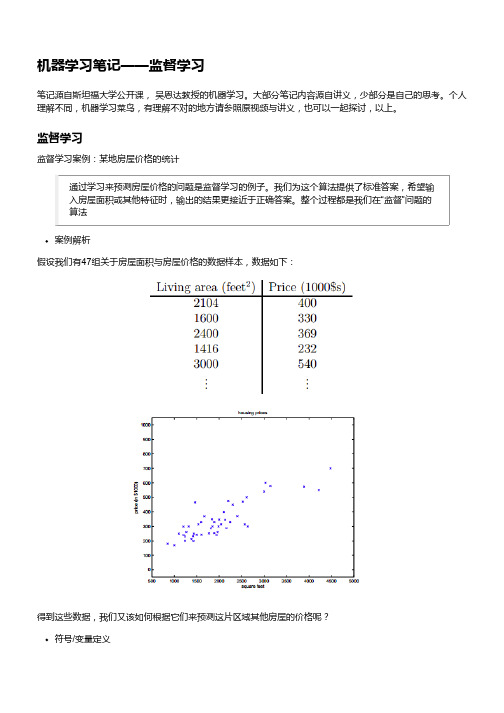
监督学习监督学习案例:某地房屋价格的统计通过学习来预测房屋价格的问题是监督学习的例子。
我们为这个算法提供了标准答案,希望输入房屋面积或其他特征时,输出的结果更接近于正确答案。
整个过程都是我们在“监督”问题的算法案例解析假设我们有47组关于房屋面积与房屋价格的数据样本,数据如下:得到这些数据,我们又该如何根据它们来预测这片区域其他房屋的价格呢?符号/变量定义函数定义我们的目的是根据现有的房屋数据,预测新的房屋数据的价格,尽量靠近真实值,而整个过程存在输入、输出、学习几个部分,如上图所示,h是将输入映射到输出上的函数。
此处的输入为房屋的面积,输出为预测得到的房屋价格。
那么h(x)就是关于真实房屋价格y的预测。
线性回归为了让案例更加有趣,我们可以为已知的数据集添加一个特征:卧室的数量。
数据集如下图所示此时的输入变量 x 是一个二维的向量,代表房屋面积,代表卧室的数量(通常情况下,设计一个学习问题中选择特征起着决定性的作用,且特征也会众多。
如何选择特征我们会在之后谈及,但是现在针对这个案例就用所给的特征)为了执行监督学习,我们必须决定如何在电脑中将我们的函数/假设表示出来。
鉴于是第一节课,所以选择比较简单的线性关系,可以用以下表达式来表示:等式中的 是参数/权重,控制着线性函数从 x 映射到 y 。
令 (不影响整个等式),简化后的等式如下等式右侧的参数 与自变量 x 都是向量,此处的符号 n 代表输入/自变量的数目(不算在其中)现在,我们得到了一组训练集,那么如何挑选、学习参数 呢?一个可行的办法似乎可以让h(x) 与 y 接近,至少是在我们当下的这些训练集中做到。
将这一做法正式化,我们将定义一个函数来进行测量,如何通过调整参数 ,让对应的 h(x) 接近相应的 y 值。
斯坦福大学机器学习笔记及代码(一)
斯坦福⼤学机器学习笔记及代码(⼀)(Notes and Codes of Machine Learning by Andrew Ng from Stanford University)说明:为了保证连贯性,⽂章按照专题⽽不是原本的课程进度来组织。
零、什么是机器学习?机器学习就是:根据已有的训练集D,采⽤学习算法A,得到特定的假设h,h能最恰当的拟合D。
h被称为最终假设,它实际上是从假设集H 中筛选的,筛选的基本要求是代价函数(cost function)最⼩。
学习算法和假设集的不同组合就构成了不同的学习模型。
简单的说,训练集D的产⽣规则符合某个函数(⽬标函数),但它难以显式(explicitly)给出,所以难以⽤⾮学习型算法实现。
学习型算法就是为了找到⼀种最恰当或最合理的⽅式来拟合这个函数,它就是最终假设h。
有了h就可以预测新的情况,进⾏分类或回归,进⽽做出决策。
⼀、线性回归线性回归在统计中是⼀种最基础的模型,也是最重要的模型,它根据给定的数据拟合出⼀条曲线来预测需要了解的情况,所⽤的算法就是最⼩⼆乘法。
机器学习以线性回归开始是合理的,与常见的知识点结合紧密,不突兀,同时破除了机器学习的⼀些神秘性,也为后续课程的展开奠定了基础,因为很多“⾮线性”的算法还是以线性算法为基础的。
1.1 假设(Hypothesis)线性回归的假设很简单,⼀元线性回归是⼆维平⾯的直线⽅程,多元线性回归则是多维空间中的平⾯(或者超平⾯):θ0+θ1x1+θ2x2+⋯+θn x n=hθ(x(i))其中,θ0的系数为1,即x0为1,写成向量形式如下:θT X=hθ(x(i))其中:X=x0x1x2⋯x nθ=θ0θ1θ2⋯θn把m个训练实例(Example)的变量X列成⼀个维度为m*(n+1)的矩阵:X=1x(1)1x(1)2⋯x(1)n1x(2)1x(2)2⋯x(2)n⋮⋮⋮x(i)j⋮1x(m)1x(m)2⋯x(m)n m×(n+1)=x(1)x(2)⋮x(m)m×1=x0x1x2⋯x n1×(n+1)其中每⾏x(i)对应⼀个训练实例,每列x j是⼀个特征(Feature),X的元素即第i个训练实例的第j个特征,可以表⽰为:x(i)j⽽假设可以进⼀步简写为:Xθ=hθ(x(1))hθ(x(2))⋯hθ(x(m))=hθ(X)1.2 代价函数(Cost Function)[][][][][][]机器学习之所以能够逐渐收敛到最终假设,就是因为每⼀次试⽤训练实例进⾏迭代时,都减⼩了代价函数的值,也就是:min J(θ)线性回归的代价函数定义为预测结果与真实值误差的平⽅和:J(θ)=12mm∑i=1(hθ(x(i))−y(i))2但是,要注意的就是代价函数不总是平⽅和,在后⾯的学习中还会接触到其他形式的代价函数。
斯坦福大学机器学习梯度算法总结

斯坦福大学机器学习梯度下降算法学习心得和相关概念介绍。
1根底概念和记号线性代数对于线性方程组可以提供一种简便的表达和操作方式,例如对于如下的方程组:4x1-5x2=13-2x1+3x2=-9可以简单的表示成下面的方式:X也是一个矩阵,为(x1,x2)T,当然你可以看成一个列向量。
1.1根本记号用A ∈表示一个矩阵A,有m行,n列,并且每一个矩阵元素都是实数。
用x ∈ , 表示一个n维向量. 通常是一个列向量. 如果要表示一个行向量的话,通常是以列向量的转置〔后面加T〕来表示。
1.2向量的积和外积根据课的定义,如果形式如xT y,或者yT x,那么表示为积,结果为一个实数,表示的是:,如果形式为xyT,那么表示的为外积:。
1.3矩阵-向量的乘法给定一个矩阵A ∈ Rm×n,以及一个向量x ∈ Rn,他们乘积为一个向量y = Ax ∈Rm。
也即如下的表示:如果A为行表示的矩阵〔即表示为〕,那么y的表示为:相对的,如果A为列表示的矩阵,那么y的表示为:即:y看成A的列的线性组合,每一列都乘以一个系数并相加,系数由x得到。
同理,yT=xT*A表示为:yT是A的行的线性组合,每一行都乘以一个系数并相加,系数由x得到。
1.4矩阵-矩阵的乘法同样有两种表示方式:第一种:A表示为行,B表示为列第二种,A表示为列,B表示为行:本质上是一样的,只是表示方式不同罢了。
1.5矩阵的梯度运算〔这是教师自定义的〕定义函数f,是从m x n矩阵到实数的一个映射,那么对于f在A上的梯度的定义如下:这里我的理解是,f〔A〕=关于A中的元素的表达式,是一个实数,然后所谓的对于A的梯度即是和A同样规模的矩阵,矩阵中的每一个元素就是f(A)针对原来的元素的求导。
1.6其他概念因为篇幅原因,所以不在这里继续赘述,其他需要的概念还有单位矩阵、对角线矩阵、矩阵转置、对称矩阵〔AT=A〕、反对称矩阵〔A=-AT〕、矩阵的迹、向量的模、线性无关、矩阵的秩、满秩矩阵、矩阵的逆〔当且仅当矩阵满秩时可逆〕、正交矩阵、矩阵的列空间(值域)、行列式、特征向量与特征值……2用到的公式在课程中用到了许多公式,罗列一下。
- 1、下载文档前请自行甄别文档内容的完整性,平台不提供额外的编辑、内容补充、找答案等附加服务。
- 2、"仅部分预览"的文档,不可在线预览部分如存在完整性等问题,可反馈申请退款(可完整预览的文档不适用该条件!)。
- 3、如文档侵犯您的权益,请联系客服反馈,我们会尽快为您处理(人工客服工作时间:9:00-18:30)。
百度文库 - 让每个人平等地提升自我1 CS 229机器学习(个人笔记)目录(1)线性回归、logistic回归和一般回归 1(2)判别模型、生成模型与朴素贝叶斯方法 10(3)支持向量机SVM(上) 20百度文库 - 让每个人平等地提升自我(4)支持向量机SVM(下) 32(5)规则化和模型选择 45(6)K-means聚类算法 50(7)混合高斯模型和EM算法 53(8)EM算法 55(9)在线学习 62(10)主成分分析 65(11)独立成分分析 80(12)线性判别分析 91(13)因子分析 103(14)增强学习 114(15)典型关联分析 120(16)偏最小二乘法回归 1292百度文库 - 让每个人平等地提升自我这里面的内容是我在2011年上半年学习斯坦福大学《机器学习》课程的个人学习笔记,内容主要来自Andrew Ng教授的讲义和学习视频。
另外也包含来自其他论文和其他学校讲义的一些内容。
每章内容主要按照个人学习时的思路总结得到。
由于是个人笔记,里面表述错误、公式错误、理解错误、笔误都会存在。
更重要的是我是初学者,千万不要认为里面的思路都正确。
如果有疑问的地方,请第一时间参考Andrew Ng教授的讲义原文和视频,再有疑问的地方可以找一些大牛问问。
博客上很多网友提出的问题,我难以回答,因为我水平确实有限,更深层次的内容最好找相关大牛咨询和相关论文研读。
如果有网友想在我这个版本基础上再添加自己的笔记,可以发送Email给我,我提供原始的word docx版本。
另,本人目前在科苑软件所读研,马上三年了,方向是分布式计算,主要偏大数据分布式处理,平时主要玩Hadoop、Pig、Hive、Mahout、NoSQL啥的,关注系统方面和数据库方面的会议。
希望大家多多交流,以后会往博客上放这些内容,机器学习会放的少了。
Anyway,祝大家学习进步、事业成功!3百度文库 - 让每个人平等地提升自我1 对回归方法的认识JerryLead2011 年2 月27 日1 摘要本报告是在学习斯坦福大学机器学习课程前四节加上配套的讲义后的总结与认识。
前四节主要讲述了回归问题,属于有监督学习中的一种方法。
该方法的核心思想是从离散的统计数据中得到数学模型,然后将该数学模型用于预测或者分类。
该方法处理的数据可以是多维的。
讲义最初介绍了一个基本问题,然后引出了线性回归的解决方法,然后针对误差问题做了概率解释。
2 问题引入假设有一个房屋销售的数据如下:x 轴是房屋的面积。
y 轴是房屋的售价,如下:百度文库 - 让每个人平等地提升自我如果来了一个新的面积,假设在销售价钱的记录中没有的,我们怎么办呢?我们可以用一条曲线去尽量准的拟合这些数据,然后如果有新的输入过来,我们可以在将曲线上这个点对应的值返回。
如果用一条直线去拟合,可能是下面的样子:绿色的点就是我们想要预测的点。
首先给出一些概念和常用的符号。
房屋销售记录表:训练集(training set)或者训练数据(training data), 是我们流程中的输入数据,一般称为x房屋销售价钱:输出数据,一般称为y拟合的函数(或者称为假设或者模型):一般写做 y = h(x)训练数据的条目数(#training set),:一条训练数据是由一对输入数据和输出数据组成的输入数据的维度n (特征的个数,#features)这个例子的特征是两维的,结果是一维的。
然而回归方法能够解决特征多维,结果是一维多离散值或一维连续值的问题。
3 学习过程下面是一个典型的机器学习的过程,首先给出一个输入数据,我们的算法会通过一系列的过程得到一个估计的函数,这个函数有能力对没有见过的新数据给出一个新的估计,也被称为构建一个模型。
就如同上面的线性回归函数。
2百度文库 - 让每个人平等地提升自我4 线性回归线性回归假设特征和结果满足线性关系。
其实线性关系的表达能力非常强大,每个特征对结果的影响强弱可以有前面的参数体现,而且每个特征变量可以首先映射到一个函数,然后再参与线性计算。
这样就可以表达特征与结果之间的非线性关系。
我们用X1,X2..Xn 去描述feature 里面的分量,比如x1=房间的面积,x2=房间的朝向,等等,我们可以做出一个估计函数:θ 在这儿称为参数,在这的意思是调整feature 中每个分量的影响力,就是到底是房屋的面积更重要还是房屋的地段更重要。
为了如果我们令X0 = 1,就可以用向量的方式来表示了:我们程序也需要一个机制去评估我们θ 是否比较好,所以说需要对我们做出的h 函数进行评估,一般这个函数称为损失函数(loss function)或者错误函数(error function),描述h 函数不好的程度,在下面,我们称这个函数为J 函数在这儿我们可以做出下面的一个错误函数:这个错误估计函数是去对x(i)的估计值与真实值y(i)差的平方和作为错误估计函数,前面乘上的1/2 是为了在求导的时候,这个系数就不见了。
3百度文库 - 让每个人平等地提升自我至于为何选择平方和作为错误估计函数,讲义后面从概率分布的角度讲解了该公式的来源。
如何调整θ 以使得J(θ)取得最小值有很多方法,其中有最小二乘法(min square),是一种完全是数学描述的方法,和梯度下降法。
5 梯度下降法在选定线性回归模型后,只需要确定参数θ,就可以将模型用来预测。
然而θ 需要在J(θ) 最小的情况下才能确定。
因此问题归结为求极小值问题,使用梯度下降法。
梯度下降法最大的问题是求得有可能是全局极小值,这与初始点的选取有关。
梯度下降法是按下面的流程进行的:1)首先对θ 赋值,这个值可以是随机的,也可以让θ 是一个全零的向量。
2)改变θ 的值,使得J(θ)按梯度下降的方向进行减少。
梯度方向由J(θ)对θ 的偏导数确定,由于求的是极小值,因此梯度方向是偏导数的反方向。
结果为迭代更新的方式有两种,一种是批梯度下降,也就是对全部的训练数据求得误差后再对θ 进行更新,另外一种是增量梯度下降,每扫描一步都要对θ 进行更新。
前一种方法能够不断收敛,后一种方法结果可能不断在收敛处徘徊。
一般来说,梯度下降法收敛速度还是比较慢的。
另一种直接计算结果的方法是最小二乘法。
6 最小二乘法将训练特征表示为X 矩阵,结果表示成y 向量,仍然是线性回归模型,误差函数不变。
那么θ 可以直接由下面公式得出4百度文库 - 让每个人平等地提升自我但此方法要求X 是列满秩的,而且求矩阵的逆比较慢。
7 选用误差函数为平方和的概率解释假设根据特征的预测结果与实际结果有误差∈(i),那么预测结果θT x(i)和真实结果y(i)满足下式:一般来讲,误差满足平均值为0 的高斯分布,也就是正态分布。
那么x 和y 的条件概率也就是这样就估计了一条样本的结果概率,然而我们期待的是模型能够在全部样本上预测最准,也就是概率积最大。
这个概率积成为最大似然估计。
我们希望在最大似然估计得到最大值时确定θ。
那么需要对最大似然估计公式求导,求导结果既是这就解释了为何误差函数要使用平方和。
当然推导过程中也做了一些假定,但这个假定符合客观规律。
8 带权重的线性回归上面提到的线性回归的误差函数里系统都是1,没有权重。
带权重的线性回归加入了权重信息。
基本假设是5百度文库 - 让每个人平等地提升自我6 其中假设w (i)符合公式其中 x 是要预测的特征,这样假设的道理是离 x 越近的样本权重越大,越远的影响越小。
这个公式与高斯分布类似,但不一样,因为w (i)不是随机变量。
此方法成为非参数学习算法,因为误差函数随着预测值的不同而不同,这样 θ 无法事先确定,预测一次需要临时计算,感觉类似 KNN 。
9 分类和对数回归一般来说,回归不用在分类问题上,因为回归是连续型模型,而且受噪声影响比较大。
如果非要应用进入,可以使用对数回归。
对数回归本质上是线性回归,只是在特征到结果的映射中加入了一层函数映射,即先把特征线性求和,然后使用函数 g(z)将最为假设函数来预测。
g(z)可以将连续值映射到 0 和 1上。
对数回归的假设函数如下,线性回归假设函数只是θT x 。
对数回归用来分类 0/1 问题,也就是预测结果属于 0 或者 1 的二值分类问题。
这里假设了二值满足伯努利分布,也就是当然假设它满足泊松分布、指数分布等等也可以,只是比较复杂,后面会提到线性回归的一般形式。
与第7 节一样,仍然求的是最大似然估计,然后求导,得到迭代公式结果为可以看到与线性回归类似,只是θT x(i)换成了ℎθ(x(i)),而ℎθ(x(i))实际上就是θT x(i)经过g(z)映射过来的。
10 牛顿法来解最大似然估计第7 和第9 节使用的解最大似然估计的方法都是求导迭代的方法,这里介绍了牛顿下降法,使结果能够快速的收敛。
当要求解f(θ) = 0时,如果f 可导,那么可以通过迭代公式来迭代求解最小值。
当应用于求解最大似然估计的最大值时,变成求解ℓ′(θ) = 0的问题。
那么迭代公式写作当θ 是向量时,牛顿法可以使用下面式子表示是n×n 的Hessian 矩阵。
牛顿法收敛速度虽然很快,但求Hessian 矩阵的逆的时候比较耗费时间。
当初始点X0 靠近极小值X 时,牛顿法的收敛速度是最快的。
但是当X0 远离极小值时,牛顿法可能不收敛,甚至连下降都保证不了。
原因是迭代点Xk+1 不一定是目标函数f 在牛顿方向上的极小点。
11 一般线性模型之所以在对数回归时使用其中的公式是由一套理论作支持的。
这个理论便是一般线性模型。
首先,如果一个概率分布可以表示成时,那么这个概率分布可以称作是指数分布。
伯努利分布,高斯分布,泊松分布,贝塔分布,狄特里特分布都属于指数分布。
在对数回归时采用的是伯努利分布,伯努利分布的概率可以表示成其中得到这就解释了对数回归时为了要用这个函数。
一般线性模型的要点是)满足一个以为参数的指数分布,那么可以求得的表达式。
)给定x,我们的目标是要确定,大多数情况下,那么我们实际上要确定的是,而。
(在对数回归中期望值是,因此h 是;在线性回归中期望值是,而高斯分布中,因此线性回归中h=)。
)12 Softmax 回归最后举了一个利用一般线性模型的例子。
假设预测值y 有k 种可能,即y 比如时,可以看作是要将一封未知邮件分为垃圾邮件、个人邮件还是工作邮件这三类。
定义那么这样即式子左边可以有其他的概率表示,因此可以当做是k-1 维的问题。
T(y)这时候一组k-1 维的向量,不再是y。
即T(y)要给出y=i(i 从1 到k-1)的概率应用于一般线性模型那么最后求得而y=i 时求得期望值那么就建立了假设函数,最后就获得了最大似然估计对该公式可以使用梯度下降或者牛顿法迭代求解。
解决了多值模型建立与预测问题。