Kernel Methods and Support Vector Machines for handwriting recgnization
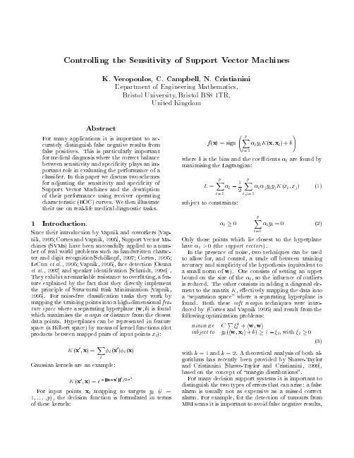
Controlling the sensitivity of support vector machines
ber of real world problems such as handwritten charac-
ter and digit recognition Scholkopf, 1997; Cortes, 1995;
LeteCalu.,n1e9t9a7l].,a1n9d9s5p;eVaakperniikd,e1n9ti95c]a, tfiaocne
cients
i are found by
L = Xp
i=1
i
?
1 2
Xp
i;j=1
i
jyiyjK(xi; xj)
(1)
subject to constraints:
i0
Xp iyi = 0
(2)
i=1
Only those points which lie closest to the hyperplane
pdoeicnitssionxifumncatpiopningis
to targets formulated
yini
(i = terms
of these kernels:
f(x) = sign
Xp
!
iyiK(x; xi) + b
i=1
where b is the bias and the coe maximising the Lagrangian:
have In
thie>p0re(stehnecesuopfpnoortisve,ecttworos
). techniques
can
be
used
to allow for, and control, a trade o between training
群智能算法优化支持向量机参数综述
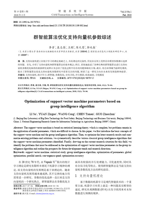
DOI : 10.11992/tis.201707011网络出版地址: /kcms/detail/23.1538.TP.20180130.1109.002.html群智能算法优化支持向量机参数综述李素1,袁志高1,王聪2,陈天恩2,郭兆春1(1. 北京工商大学 食品安全大数据技术北京市重点实验室,北京 100048; 2. 国家农业信息化工程技术研究中心,北京 100097)摘 要:支持向量机建立在统计学习的理论基础之上,具有理论的完备性,但是在应用上仍然存在模型参数难以选择的问题。
首先,介绍了支持向量机和群智能算法的基本概念;然后,系统地叙述了各种经典的群智能算法进行支持向量机参数优化取得的最新研究成果以及总结了优化过程中存在的问题和解决方案;最后,结合该领域当前研究现状,提出了群智能算法优化支持向量机参数研究中需要关注的问题,展望了这一研究方向在未来的发展趋势和前景。
关键词:支持向量机;统计学习;群智能;参数优化;全局寻优;并行搜索;收敛速度;寻优精度中图分类号:TP181 文献标志码:A 文章编号:1673−4785(2018)01−0070−15中文引用格式:李素, 袁志高, 王聪, 等. 群智能算法优化支持向量机参数综述[J]. 智能系统学报, 2018, 13(1): 70–84.英文引用格式:LI Su, YUAN Zhigao, WANG Cong, et al. Optimization of support vector machine parameters based on group in-telligence algorithm[J]. CAAI transactions on intelligent systems, 2018, 13(1): 70–84.Optimization of support vector machine parameters based ongroup intelligence algorithmLI Su 1,YUAN Zhigao 1,WANG Cong 2,CHEN Tianen 2,GUO Zhaochun 1(1. Beijing Key Laboratory of Big Data Technology for Food Safety, Beijing Technology and Business University, Beijing 100048,China; 2. National Engineering Research Center for Information Technology in Agriculture, Beijing 100097, China)Abstract : The support vector machine is based on statistical learning theory, which is complete, but problems remain in the application of model parameters, which are difficult to choose. In this paper, we first introduce the basic concepts of the support vector machine and the group intelligence algorithm. Then, to optimize the latest research results and sum-marize existing problems and solutions, we systematically describe various classical group intelligence algorithms that the support vector machine parameters identified. Finally, drawing on the current research situation for this field, we identify the problems that must be addressed in the optimization of support vector machine parameters in the group in-telligence algorithm and outline the prospects for future development trends and research directions.Keywords : support vector machine; statistical study; group intelligence algorithm; optimization of parameters; global optimization; parallel search; convergence speed; optimization accuracy在20世纪70年代,由Vapnik 等[1]提出的统计学习理论是研究有限样本情况下机器学习规律的理论,而支持向量机的发展则是基于该理论的。
An Introduction to Support Vector Machines
9/13/2013
Input space 802. Prepared by Martin LawFeature space CSE
Example Transformation
Define the kernel function K (x,y) as Consider the following transformation
9/13/2013
CSE 802. Prepared by Martin Law
7
The Optimization Problem the problem to its dual
This is a quadratic programming (QP) problem
Kernel methods, large margin classifiers, reproducing kernel Hilbert space, Gaussian process
CSE 802. Prepared by Martin Law 3
9/13/2013
Two Class Problem: Linear Separable Case
Global maximum of ai can always be found
w can be recovered by
CSE 802. Prepared by Martin Law 8
9/13/2013
Characteristics of the Solution
Many of the ai are zero
Class 2
Many decision boundaries can separate these two classes Which one should we choose?
Support Vector Machines for Classification and Regression
UNIVERSITY OF SOUTHAMPTONSupport Vector MachinesforClassification and RegressionbySteve R.GunnTechnical ReportFaculty of Engineering,Science and Mathematics School of Electronics and Computer Science10May1998ContentsNomenclature xi1Introduction11.1Statistical Learning Theory (2)1.1.1VC Dimension (3)1.1.2Structural Risk Minimisation (4)2Support Vector Classification52.1The Optimal Separating Hyperplane (5)2.1.1Linearly Separable Example (10)2.2The Generalised Optimal Separating Hyperplane (10)2.2.1Linearly Non-Separable Example (13)2.3Generalisation in High Dimensional Feature Space (14)2.3.1Polynomial Mapping Example (16)2.4Discussion (16)3Feature Space193.1Kernel Functions (19)3.1.1Polynomial (20)3.1.2Gaussian Radial Basis Function (20)3.1.3Exponential Radial Basis Function (20)3.1.4Multi-Layer Perceptron (20)3.1.5Fourier Series (21)3.1.6Splines (21)3.1.7B splines (21)3.1.8Additive Kernels (22)3.1.9Tensor Product (22)3.2Implicit vs.Explicit Bias (22)3.3Data Normalisation (23)3.4Kernel Selection (23)4Classification Example:IRIS data254.1Applications (28)5Support Vector Regression295.1Linear Regression (30)5.1.1 -insensitive Loss Function (30)5.1.2Quadratic Loss Function (31)iiiiv CONTENTS5.1.3Huber Loss Function (32)5.1.4Example (33)5.2Non Linear Regression (33)5.2.1Examples (34)5.2.2Comments (36)6Regression Example:Titanium Data396.1Applications (42)7Conclusions43A Implementation Issues45A.1Support Vector Classification (45)A.2Support Vector Regression (47)B MATLAB SVM Toolbox51 Bibliography53List of Figures1.1Modelling Errors (2)1.2VC Dimension Illustration (3)2.1Optimal Separating Hyperplane (5)2.2Canonical Hyperplanes (6)2.3Constraining the Canonical Hyperplanes (7)2.4Optimal Separating Hyperplane (10)2.5Generalised Optimal Separating Hyperplane (11)2.6Generalised Optimal Separating Hyperplane Example(C=1) (13)2.7Generalised Optimal Separating Hyperplane Example(C=105) (14)2.8Generalised Optimal Separating Hyperplane Example(C=10−8) (14)2.9Mapping the Input Space into a High Dimensional Feature Space (14)2.10Mapping input space into Polynomial Feature Space (16)3.1Comparison between Implicit and Explicit bias for a linear kernel (22)4.1Iris data set (25)4.2Separating Setosa with a linear SVC(C=∞) (26)4.3Separating Viginica with a polynomial SVM(degree2,C=∞) (26)4.4Separating Viginica with a polynomial SVM(degree10,C=∞) (26)4.5Separating Viginica with a Radial Basis Function SVM(σ=1.0,C=∞)274.6Separating Viginica with a polynomial SVM(degree2,C=10) (27)4.7The effect of C on the separation of Versilcolor with a linear spline SVM.285.1Loss Functions (29)5.2Linear regression (33)5.3Polynomial Regression (35)5.4Radial Basis Function Regression (35)5.5Spline Regression (36)5.6B-spline Regression (36)5.7Exponential RBF Regression (36)6.1Titanium Linear Spline Regression( =0.05,C=∞) (39)6.2Titanium B-Spline Regression( =0.05,C=∞) (40)6.3Titanium Gaussian RBF Regression( =0.05,σ=1.0,C=∞) (40)6.4Titanium Gaussian RBF Regression( =0.05,σ=0.3,C=∞) (40)6.5Titanium Exponential RBF Regression( =0.05,σ=1.0,C=∞) (41)6.6Titanium Fourier Regression( =0.05,degree3,C=∞) (41)6.7Titanium Linear Spline Regression( =0.05,C=10) (42)vvi LIST OF FIGURES6.8Titanium B-Spline Regression( =0.05,C=10) (42)List of Tables2.1Linearly Separable Classification Data (10)2.2Non-Linearly Separable Classification Data (13)5.1Regression Data (33)viiListingsA.1Support Vector Classification MATLAB Code (46)A.2Support Vector Regression MATLAB Code (48)ixNomenclature0Column vector of zeros(x)+The positive part of xC SVM misclassification tolerance parameterD DatasetK(x,x )Kernel functionR[f]Risk functionalR emp[f]Empirical Risk functionalxiChapter1IntroductionThe problem of empirical data modelling is germane to many engineering applications. In empirical data modelling a process of induction is used to build up a model of the system,from which it is hoped to deduce responses of the system that have yet to be ob-served.Ultimately the quantity and quality of the observations govern the performance of this empirical model.By its observational nature data obtained isfinite and sampled; typically this sampling is non-uniform and due to the high dimensional nature of the problem the data will form only a sparse distribution in the input space.Consequently the problem is nearly always ill posed(Poggio et al.,1985)in the sense of Hadamard (Hadamard,1923).Traditional neural network approaches have suffered difficulties with generalisation,producing models that can overfit the data.This is a consequence of the optimisation algorithms used for parameter selection and the statistical measures used to select the’best’model.The foundations of Support Vector Machines(SVM)have been developed by Vapnik(1995)and are gaining popularity due to many attractive features,and promising empirical performance.The formulation embodies the Struc-tural Risk Minimisation(SRM)principle,which has been shown to be superior,(Gunn et al.,1997),to traditional Empirical Risk Minimisation(ERM)principle,employed by conventional neural networks.SRM minimises an upper bound on the expected risk, as opposed to ERM that minimises the error on the training data.It is this difference which equips SVM with a greater ability to generalise,which is the goal in statistical learning.SVMs were developed to solve the classification problem,but recently they have been extended to the domain of regression problems(Vapnik et al.,1997).In the literature the terminology for SVMs can be slightly confusing.The term SVM is typ-ically used to describe classification with support vector methods and support vector regression is used to describe regression with support vector methods.In this report the term SVM will refer to both classification and regression methods,and the terms Support Vector Classification(SVC)and Support Vector Regression(SVR)will be used for specification.This section continues with a brief introduction to the structural risk12Chapter1Introductionminimisation principle.In Chapter2the SVM is introduced in the setting of classifica-tion,being both historical and more accessible.This leads onto mapping the input into a higher dimensional feature space by a suitable choice of kernel function.The report then considers the problem of regression.Illustrative examples re given to show the properties of the techniques.1.1Statistical Learning TheoryThis section is a very brief introduction to statistical learning theory.For a much more in depth look at statistical learning theory,see(Vapnik,1998).Figure1.1:Modelling ErrorsThe goal in modelling is to choose a model from the hypothesis space,which is closest (with respect to some error measure)to the underlying function in the target space. Errors in doing this arise from two cases:Approximation Error is a consequence of the hypothesis space being smaller than the target space,and hence the underlying function may lie outside the hypothesis space.A poor choice of the model space will result in a large approximation error, and is referred to as model mismatch.Estimation Error is the error due to the learning procedure which results in a tech-nique selecting the non-optimal model from the hypothesis space.Chapter1Introduction3Together these errors form the generalisation error.Ultimately we would like tofind the function,f,which minimises the risk,R[f]=X×YL(y,f(x))P(x,y)dxdy(1.1)However,P(x,y)is unknown.It is possible tofind an approximation according to the empirical risk minimisation principle,R emp[f]=1lli=1Ly i,fx i(1.2)which minimises the empirical risk,ˆf n,l (x)=arg minf∈H nR emp[f](1.3)Empirical risk minimisation makes sense only if,liml→∞R emp[f]=R[f](1.4) which is true from the law of large numbers.However,it must also satisfy,lim l→∞minf∈H nR emp[f]=minf∈H nR[f](1.5)which is only valid when H n is’small’enough.This condition is less intuitive and requires that the minima also converge.The following bound holds with probability1−δ,R[f]≤R emp[f]+h ln2lh+1−lnδ4l(1.6)Remarkably,this expression for the expected risk is independent of the probability dis-tribution.1.1.1VC DimensionThe VC dimension is a scalar value that measures the capacity of a set offunctions.Figure1.2:VC Dimension Illustration4Chapter1IntroductionDefinition1.1(Vapnik–Chervonenkis).The VC dimension of a set of functions is p if and only if there exists a set of points{x i}pi=1such that these points can be separatedin all2p possible configurations,and that no set{x i}qi=1exists where q>p satisfying this property.Figure1.2illustrates how three points in the plane can be shattered by the set of linear indicator functions whereas four points cannot.In this case the VC dimension is equal to the number of free parameters,but in general that is not the case;e.g.the function A sin(bx)has an infinite VC dimension(Vapnik,1995).The set of linear indicator functions in n dimensional space has a VC dimension equal to n+1.1.1.2Structural Risk MinimisationCreate a structure such that S h is a hypothesis space of VC dimension h then,S1⊂S2⊂...⊂S∞(1.7) SRM consists in solving the following problemmin S h R emp[f]+h ln2lh+1−lnδ4l(1.8)If the underlying process being modelled is not deterministic the modelling problem becomes more exacting and consequently this chapter is restricted to deterministic pro-cesses.Multiple output problems can usually be reduced to a set of single output prob-lems that may be considered independent.Hence it is appropriate to consider processes with multiple inputs from which it is desired to predict a single output.Chapter2Support Vector ClassificationThe classification problem can be restricted to consideration of the two-class problem without loss of generality.In this problem the goal is to separate the two classes by a function which is induced from available examples.The goal is to produce a classifier that will work well on unseen examples,i.e.it generalises well.Consider the example in Figure2.1.Here there are many possible linear classifiers that can separate the data, but there is only one that maximises the margin(maximises the distance between it and the nearest data point of each class).This linear classifier is termed the optimal separating hyperplane.Intuitively,we would expect this boundary to generalise well as opposed to the other possible boundaries.Figure2.1:Optimal Separating Hyperplane2.1The Optimal Separating HyperplaneConsider the problem of separating the set of training vectors belonging to two separateclasses,D=(x1,y1),...,(x l,y l),x∈R n,y∈{−1,1},(2.1)56Chapter 2Support Vector Classificationwith a hyperplane, w,x +b =0.(2.2)The set of vectors is said to be optimally separated by the hyperplane if it is separated without error and the distance between the closest vector to the hyperplane is maximal.There is some redundancy in Equation 2.2,and without loss of generality it is appropri-ate to consider a canonical hyperplane (Vapnik ,1995),where the parameters w ,b are constrained by,min i w,x i +b =1.(2.3)This incisive constraint on the parameterisation is preferable to alternatives in simpli-fying the formulation of the problem.In words it states that:the norm of the weight vector should be equal to the inverse of the distance,of the nearest point in the data set to the hyperplane .The idea is illustrated in Figure 2.2,where the distance from the nearest point to each hyperplane is shown.Figure 2.2:Canonical HyperplanesA separating hyperplane in canonical form must satisfy the following constraints,y i w,x i +b ≥1,i =1,...,l.(2.4)The distance d (w,b ;x )of a point x from the hyperplane (w,b )is,d (w,b ;x )= w,x i +bw .(2.5)Chapter 2Support Vector Classification 7The optimal hyperplane is given by maximising the margin,ρ,subject to the constraints of Equation 2.4.The margin is given by,ρ(w,b )=min x i :y i =−1d (w,b ;x i )+min x i :y i =1d (w,b ;x i )=min x i :y i =−1 w,x i +b w +min x i :y i =1 w,x i +b w =1 w min x i :y i =−1 w,x i +b +min x i :y i =1w,x i +b =2 w (2.6)Hence the hyperplane that optimally separates the data is the one that minimisesΦ(w )=12 w 2.(2.7)It is independent of b because provided Equation 2.4is satisfied (i.e.it is a separating hyperplane)changing b will move it in the normal direction to itself.Accordingly the margin remains unchanged but the hyperplane is no longer optimal in that it will be nearer to one class than the other.To consider how minimising Equation 2.7is equivalent to implementing the SRM principle,suppose that the following bound holds,w <A.(2.8)Then from Equation 2.4and 2.5,d (w,b ;x )≥1A.(2.9)Accordingly the hyperplanes cannot be nearer than 1A to any of the data points and intuitively it can be seen in Figure 2.3how this reduces the possible hyperplanes,andhence thecapacity.Figure 2.3:Constraining the Canonical Hyperplanes8Chapter2Support Vector ClassificationThe VC dimension,h,of the set of canonical hyperplanes in n dimensional space is bounded by,h≤min[R2A2,n]+1,(2.10)where R is the radius of a hypersphere enclosing all the data points.Hence minimising Equation2.7is equivalent to minimising an upper bound on the VC dimension.The solution to the optimisation problem of Equation2.7under the constraints of Equation 2.4is given by the saddle point of the Lagrange functional(Lagrangian)(Minoux,1986),Φ(w,b,α)=12 w 2−li=1αiy iw,x i +b−1,(2.11)whereαare the Lagrange multipliers.The Lagrangian has to be minimised with respect to w,b and maximised with respect toα≥0.Classical Lagrangian duality enables the primal problem,Equation2.11,to be transformed to its dual problem,which is easier to solve.The dual problem is given by,max αW(α)=maxαminw,bΦ(w,b,α).(2.12)The minimum with respect to w and b of the Lagrangian,Φ,is given by,∂Φ∂b =0⇒li=1αi y i=0∂Φ∂w =0⇒w=li=1αi y i x i.(2.13)Hence from Equations2.11,2.12and2.13,the dual problem is,max αW(α)=maxα−12li=1lj=1αiαj y i y j x i,x j +lk=1αk,(2.14)and hence the solution to the problem is given by,α∗=arg minα12li=1lj=1αiαj y i y j x i,x j −lk=1αk,(2.15)with constraints,αi≥0i=1,...,llj=1αj y j=0.(2.16)Chapter2Support Vector Classification9Solving Equation2.15with constraints Equation2.16determines the Lagrange multi-pliers,and the optimal separating hyperplane is given by,w∗=li=1αi y i x ib∗=−12w∗,x r+x s .(2.17)where x r and x s are any support vector from each class satisfying,αr,αs>0,y r=−1,y s=1.(2.18)The hard classifier is then,f(x)=sgn( w∗,x +b)(2.19) Alternatively,a soft classifier may be used which linearly interpolates the margin,f(x)=h( w∗,x +b)where h(z)=−1:z<−1z:−1≤z≤1+1:z>1(2.20)This may be more appropriate than the hard classifier of Equation2.19,because it produces a real valued output between−1and1when the classifier is queried within the margin,where no training data resides.From the Kuhn-Tucker conditions,αiy iw,x i +b−1=0,i=1,...,l,(2.21)and hence only the points x i which satisfy,y iw,x i +b=1(2.22)will have non-zero Lagrange multipliers.These points are termed Support Vectors(SV). If the data is linearly separable all the SV will lie on the margin and hence the number of SV can be very small.Consequently the hyperplane is determined by a small subset of the training set;the other points could be removed from the training set and recalculating the hyperplane would produce the same answer.Hence SVM can be used to summarise the information contained in a data set by the SV produced.If the data is linearly separable the following equality will hold,w 2=li=1αi=i∈SV sαi=i∈SV sj∈SV sαiαj y i y j x i,x j .(2.23)Hence from Equation2.10the VC dimension of the classifier is bounded by,h≤min[R2i∈SV s,n]+1,(2.24)10Chapter2Support Vector Classificationx1x2y11-133113131-12 2.513 2.5-143-1Table2.1:Linearly Separable Classification Dataand if the training data,x,is normalised to lie in the unit hypersphere,,n],(2.25)h≤1+min[i∈SV s2.1.1Linearly Separable ExampleTo illustrate the method consider the training set in Table2.1.The SVC solution is shown in Figure2.4,where the dotted lines describe the locus of the margin and the circled data points represent the SV,which all lie on the margin.Figure2.4:Optimal Separating Hyperplane2.2The Generalised Optimal Separating HyperplaneSo far the discussion has been restricted to the case where the training data is linearly separable.However,in general this will not be the case,Figure2.5.There are two approaches to generalising the problem,which are dependent upon prior knowledge of the problem and an estimate of the noise on the data.In the case where it is expected (or possibly even known)that a hyperplane can correctly separate the data,a method ofChapter2Support Vector Classification11Figure2.5:Generalised Optimal Separating Hyperplaneintroducing an additional cost function associated with misclassification is appropriate. Alternatively a more complex function can be used to describe the boundary,as discussed in Chapter2.1.To enable the optimal separating hyperplane method to be generalised, Cortes and Vapnik(1995)introduced non-negative variables,ξi≥0,and a penalty function,Fσ(ξ)=iξσiσ>0,(2.26) where theξi are a measure of the misclassification errors.The optimisation problem is now posed so as to minimise the classification error as well as minimising the bound on the VC dimension of the classifier.The constraints of Equation2.4are modified for the non-separable case to,y iw,x i +b≥1−ξi,i=1,...,l.(2.27)whereξi≥0.The generalised optimal separating hyperplane is determined by the vector w,that minimises the functional,Φ(w,ξ)=12w 2+Ciξi,(2.28)(where C is a given value)subject to the constraints of Equation2.27.The solution to the optimisation problem of Equation2.28under the constraints of Equation2.27is given by the saddle point of the Lagrangian(Minoux,1986),Φ(w,b,α,ξ,β)=12 w 2+Ciξi−li=1αiy iw T x i+b−1+ξi−lj=1βiξi,(2.29)12Chapter2Support Vector Classificationwhereα,βare the Lagrange multipliers.The Lagrangian has to be minimised with respect to w,b,x and maximised with respect toα,β.As before,classical Lagrangian duality enables the primal problem,Equation2.29,to be transformed to its dual problem. The dual problem is given by,max αW(α,β)=maxα,βminw,b,ξΦ(w,b,α,ξ,β).(2.30)The minimum with respect to w,b andξof the Lagrangian,Φ,is given by,∂Φ∂b =0⇒li=1αi y i=0∂Φ∂w =0⇒w=li=1αi y i x i∂Φ∂ξ=0⇒αi+βi=C.(2.31) Hence from Equations2.29,2.30and2.31,the dual problem is,max αW(α)=maxα−12li=1lj=1αiαj y i y j x i,x j +lk=1αk,(2.32)and hence the solution to the problem is given by,α∗=arg minα12li=1lj=1αiαj y i y j x i,x j −lk=1αk,(2.33)with constraints,0≤αi≤C i=1,...,llj=1αj y j=0.(2.34)The solution to this minimisation problem is identical to the separable case except for a modification of the bounds of the Lagrange multipliers.The uncertain part of Cortes’s approach is that the coefficient C has to be determined.This parameter introduces additional capacity control within the classifier.C can be directly related to a regulari-sation parameter(Girosi,1997;Smola and Sch¨o lkopf,1998).Blanz et al.(1996)uses a value of C=5,but ultimately C must be chosen to reflect the knowledge of the noise on the data.This warrants further work,but a more practical discussion is given in Chapter4.Chapter2Support Vector Classification13x1x2y11-133113131-12 2.513 2.5-143-11.5 1.5112-1Table2.2:Non-Linearly Separable Classification Data2.2.1Linearly Non-Separable ExampleTwo additional data points are added to the separable data of Table2.1to produce a linearly non-separable data set,Table2.2.The resulting SVC is shown in Figure2.6,for C=1.The SV are no longer required to lie on the margin,as in Figure2.4,and the orientation of the hyperplane and the width of the margin are different.Figure2.6:Generalised Optimal Separating Hyperplane Example(C=1)In the limit,lim C→∞the solution converges towards the solution obtained by the optimal separating hyperplane(on this non-separable data),Figure2.7.In the limit,lim C→0the solution converges to one where the margin maximisation term dominates,Figure2.8.Beyond a certain point the Lagrange multipliers will all take on the value of C.There is now less emphasis on minimising the misclassification error, but purely on maximising the margin,producing a large width margin.Consequently as C decreases the width of the margin increases.The useful range of C lies between the point where all the Lagrange Multipliers are equal to C and when only one of them is just bounded by C.14Chapter2Support Vector ClassificationFigure2.7:Generalised Optimal Separating Hyperplane Example(C=105)Figure2.8:Generalised Optimal Separating Hyperplane Example(C=10−8)2.3Generalisation in High Dimensional Feature SpaceIn the case where a linear boundary is inappropriate the SVM can map the input vector, x,into a high dimensional feature space,z.By choosing a non-linear mapping a priori, the SVM constructs an optimal separating hyperplane in this higher dimensional space, Figure2.9.The idea exploits the method of Aizerman et al.(1964)which,enables the curse of dimensionality(Bellman,1961)to be addressed.Figure2.9:Mapping the Input Space into a High Dimensional Feature SpaceChapter2Support Vector Classification15There are some restrictions on the non-linear mapping that can be employed,see Chap-ter3,but it turns out,surprisingly,that most commonly employed functions are accept-able.Among acceptable mappings are polynomials,radial basis functions and certain sigmoid functions.The optimisation problem of Equation2.33becomes,α∗=arg minα12li=1lj=1αiαj y i y j K(x i,x j)−lk=1αk,(2.35)where K(x,x )is the kernel function performing the non-linear mapping into feature space,and the constraints are unchanged,0≤αi≤C i=1,...,llj=1αj y j=0.(2.36)Solving Equation2.35with constraints Equation2.36determines the Lagrange multipli-ers,and a hard classifier implementing the optimal separating hyperplane in the feature space is given by,f(x)=sgn(i∈SV sαi y i K(x i,x)+b)(2.37) wherew∗,x =li=1αi y i K(x i,x)b∗=−12li=1αi y i[K(x i,x r)+K(x i,x r)].(2.38)The bias is computed here using two support vectors,but can be computed using all the SV on the margin for stability(Vapnik et al.,1997).If the Kernel contains a bias term, the bias can be accommodated within the Kernel,and hence the classifier is simply,f(x)=sgn(i∈SV sαi K(x i,x))(2.39)Many employed kernels have a bias term and anyfinite Kernel can be made to have one(Girosi,1997).This simplifies the optimisation problem by removing the equality constraint of Equation2.36.Chapter3discusses the necessary conditions that must be satisfied by valid kernel functions.16Chapter2Support Vector Classification 2.3.1Polynomial Mapping ExampleConsider a polynomial kernel of the form,K(x,x )=( x,x +1)2,(2.40)which maps a two dimensional input vector into a six dimensional feature space.Apply-ing the non-linear SVC to the linearly non-separable training data of Table2.2,produces the classification illustrated in Figure2.10(C=∞).The margin is no longer of constant width due to the non-linear projection into the input space.The solution is in contrast to Figure2.7,in that the training data is now classified correctly.However,even though SVMs implement the SRM principle and hence can generalise well,a careful choice of the kernel function is necessary to produce a classification boundary that is topologically appropriate.It is always possible to map the input space into a dimension greater than the number of training points and produce a classifier with no classification errors on the training set.However,this will generalise badly.Figure2.10:Mapping input space into Polynomial Feature Space2.4DiscussionTypically the data will only be linearly separable in some,possibly very high dimensional feature space.It may not make sense to try and separate the data exactly,particularly when only afinite amount of training data is available which is potentially corrupted by noise.Hence in practice it will be necessary to employ the non-separable approach which places an upper bound on the Lagrange multipliers.This raises the question of how to determine the parameter C.It is similar to the problem in regularisation where the regularisation coefficient has to be determined,and it has been shown that the parameter C can be directly related to a regularisation parameter for certain kernels (Smola and Sch¨o lkopf,1998).A process of cross-validation can be used to determine thisChapter2Support Vector Classification17parameter,although more efficient and potentially better methods are sought after.In removing the training patterns that are not support vectors,the solution is unchanged and hence a fast method for validation may be available when the support vectors are sparse.Chapter3Feature SpaceThis chapter discusses the method that can be used to construct a mapping into a high dimensional feature space by the use of reproducing kernels.The idea of the kernel function is to enable operations to be performed in the input space rather than the potentially high dimensional feature space.Hence the inner product does not need to be evaluated in the feature space.This provides a way of addressing the curse of dimensionality.However,the computation is still critically dependent upon the number of training patterns and to provide a good data distribution for a high dimensional problem will generally require a large training set.3.1Kernel FunctionsThe following theory is based upon Reproducing Kernel Hilbert Spaces(RKHS)(Aron-szajn,1950;Girosi,1997;Heckman,1997;Wahba,1990).An inner product in feature space has an equivalent kernel in input space,K(x,x )= φ(x),φ(x ) ,(3.1)provided certain conditions hold.If K is a symmetric positive definite function,which satisfies Mercer’s Conditions,K(x,x )=∞ma mφm(x)φm(x ),a m≥0,(3.2)K(x,x )g(x)g(x )dxdx >0,g∈L2,(3.3) then the kernel represents a legitimate inner product in feature space.Valid functions that satisfy Mercer’s conditions are now given,which unless stated are valid for all real x and x .1920Chapter3Feature Space3.1.1PolynomialA polynomial mapping is a popular method for non-linear modelling,K(x,x )= x,x d.(3.4)K(x,x )=x,x +1d.(3.5)The second kernel is usually preferable as it avoids problems with the hessian becoming zero.3.1.2Gaussian Radial Basis FunctionRadial basis functions have received significant attention,most commonly with a Gaus-sian of the form,K(x,x )=exp−x−x 22σ2.(3.6)Classical techniques utilising radial basis functions employ some method of determining a subset of centres.Typically a method of clustering isfirst employed to select a subset of centres.An attractive feature of the SVM is that this selection is implicit,with each support vectors contributing one local Gaussian function,centred at that data point. By further considerations it is possible to select the global basis function width,s,using the SRM principle(Vapnik,1995).3.1.3Exponential Radial Basis FunctionA radial basis function of the form,K(x,x )=exp−x−x2σ2.(3.7)produces a piecewise linear solution which can be attractive when discontinuities are acceptable.3.1.4Multi-Layer PerceptronThe long established MLP,with a single hidden layer,also has a valid kernel represen-tation,K(x,x )=tanhρ x,x +(3.8)for certain values of the scale,ρ,and offset, ,parameters.Here the SV correspond to thefirst layer and the Lagrange multipliers to the weights.。
支持向量机(SVM)简介
D(x, y) = K( x, x) + K( y, y) − 2K( x, y)
核函数构造
机器学习和模式识别中的很多算法要求输入模式是向 量空间中的元素。 但是,输入模式可能是非向量的形式,可能是任何对 象——串、树,图、蛋白质结构、人… 一种做法:把对象表示成向量的形式,传统算法得以 应用。 问题:在有些情况下,很难把关于事物的直观认识抽 象成向量形式。比如,文本分类问题。或者构造的向 量维度非常高,以至于无法进行运算。
学习问题
学习问题就是从给定的函数集f(x,w),w W中选择出 ∈ 能够最好的近训练器响应的函数。而这种选择是 基于训练集的,训练集由根据联合分布 F(x,y)=F(x)F(y|x)抽取的n个独立同分布样本 (xi,yi), i=1,2,…,n 组成 。
学习问题的表示
学习的目的就是,在联合概率分布函数F(x,y)未知、 所有可用的信息都包含在训练集中的情况下,寻找 函数f(x,w0),使它(在函数类f(x,w),(w W)上 最小化风险泛函
支持向量机(SVM)简介
付岩
2007年6月12日
提纲
统计学习理论基本思想 标准形式的分类SVM 核函数技术 SVM快速实现算法 SVM的一些扩展形式
学习问题
x G S LM y _ y
x∈ Rn,它带有一定 产生器(G),随机产生向量
但未知的概率分布函数F(x) 训练器(S),条件概率分布函数F(y|x) ,期望响应y 和输入向量x关系为y=f(x,v) 学习机器(LM),输入-输出映射函数集y=f(x,w), ∈ w W,W是参数集合。
核函数构造
String matching kernel
定义:
K( x, x′) =
Support vector machine_A tool for mapping mineral prospectivity
Support vector machine:A tool for mapping mineral prospectivityRenguang Zuo a,n,Emmanuel John M.Carranza ba State Key Laboratory of Geological Processes and Mineral Resources,China University of Geosciences,Wuhan430074;Beijing100083,Chinab Department of Earth Systems Analysis,Faculty of Geo-Information Science and Earth Observation(ITC),University of Twente,Enschede,The Netherlandsa r t i c l e i n f oArticle history:Received17May2010Received in revised form3September2010Accepted25September2010Keywords:Supervised learning algorithmsKernel functionsWeights-of-evidenceTurbidite-hosted AuMeguma Terraina b s t r a c tIn this contribution,we describe an application of support vector machine(SVM),a supervised learningalgorithm,to mineral prospectivity mapping.The free R package e1071is used to construct a SVM withsigmoid kernel function to map prospectivity for Au deposits in western Meguma Terrain of Nova Scotia(Canada).The SVM classification accuracies of‘deposit’are100%,and the SVM classification accuracies ofthe‘non-deposit’are greater than85%.The SVM classifications of mineral prospectivity have5–9%lowertotal errors,13–14%higher false-positive errors and25–30%lower false-negative errors compared tothose of the WofE prediction.The prospective target areas predicted by both SVM and WofE reflect,nonetheless,controls of Au deposit occurrence in the study area by NE–SW trending anticlines andcontact zones between Goldenville and Halifax Formations.The results of the study indicate theusefulness of SVM as a tool for predictive mapping of mineral prospectivity.&2010Elsevier Ltd.All rights reserved.1.IntroductionMapping of mineral prospectivity is crucial in mineral resourcesexploration and mining.It involves integration of information fromdiverse geoscience datasets including geological data(e.g.,geologicalmap),geochemical data(e.g.,stream sediment geochemical data),geophysical data(e.g.,magnetic data)and remote sensing data(e.g.,multispectral satellite data).These sorts of data can be visualized,processed and analyzed with the support of computer and GIStechniques.Geocomputational techniques for mapping mineral pro-spectivity include weights of evidence(WofE)(Bonham-Carter et al.,1989),fuzzy WofE(Cheng and Agterberg,1999),logistic regression(Agterberg and Bonham-Carter,1999),fuzzy logic(FL)(Ping et al.,1991),evidential belief functions(EBF)(An et al.,1992;Carranza andHale,2003;Carranza et al.,2005),neural networks(NN)(Singer andKouda,1996;Porwal et al.,2003,2004),a‘wildcat’method(Carranza,2008,2010;Carranza and Hale,2002)and a hybrid method(e.g.,Porwalet al.,2006;Zuo et al.,2009).These techniques have been developed toquantify indices of occurrence of mineral deposit occurrence byintegrating multiple evidence layers.Some geocomputational techni-ques can be performed using popular software packages,such asArcWofE(a free ArcView extension)(Kemp et al.,1999),ArcSDM9.3(afree ArcGIS9.3extension)(Sawatzky et al.,2009),MI-SDM2.50(aMapInfo extension)(Avantra Geosystems,2006),GeoDAS(developedbased on MapObjects,which is an Environmental Research InstituteDevelopment Kit)(Cheng,2000).Other geocomputational techniques(e.g.,FL and NN)can be performed by using R and Matlab.Geocomputational techniques for mineral prospectivity map-ping can be categorized generally into two types–knowledge-driven and data-driven–according to the type of inferencemechanism considered(Bonham-Carter1994;Pan and Harris2000;Carranza2008).Knowledge-driven techniques,such as thosethat apply FL and EBF,are based on expert knowledge andexperience about spatial associations between mineral prospec-tivity criteria and mineral deposits of the type sought.On the otherhand,data-driven techniques,such as WofE and NN,are based onthe quantification of spatial associations between mineral pro-spectivity criteria and known occurrences of mineral deposits ofthe type sought.Additional,the mixing of knowledge-driven anddata-driven methods also is used for mapping of mineral prospec-tivity(e.g.,Porwal et al.,2006;Zuo et al.,2009).Every geocomputa-tional technique has advantages and disadvantages,and one or theother may be more appropriate for a given geologic environmentand exploration scenario(Harris et al.,2001).For example,one ofthe advantages of WofE is its simplicity,and straightforwardinterpretation of the weights(Pan and Harris,2000),but thismodel ignores the effects of possible correlations amongst inputpredictor patterns,which generally leads to biased prospectivitymaps by assuming conditional independence(Porwal et al.,2010).Comparisons between WofE and NN,NN and LR,WofE,NN and LRfor mineral prospectivity mapping can be found in Singer andKouda(1999),Harris and Pan(1999)and Harris et al.(2003),respectively.Mapping of mineral prospectivity is a classification process,because its product(i.e.,index of mineral deposit occurrence)forevery location is classified as either prospective or non-prospectiveaccording to certain combinations of weighted mineral prospec-tivity criteria.There are two types of classification techniques.Contents lists available at ScienceDirectjournal homepage:/locate/cageoComputers&Geosciences0098-3004/$-see front matter&2010Elsevier Ltd.All rights reserved.doi:10.1016/j.cageo.2010.09.014n Corresponding author.E-mail addresses:zrguang@,zrguang1981@(R.Zuo).Computers&Geosciences](]]]])]]]–]]]One type is known as supervised classification,which classifies mineral prospectivity of every location based on a training set of locations of known deposits and non-deposits and a set of evidential data layers.The other type is known as unsupervised classification, which classifies mineral prospectivity of every location based solely on feature statistics of individual evidential data layers.A support vector machine(SVM)is a model of algorithms for supervised classification(Vapnik,1995).Certain types of SVMs have been developed and applied successfully to text categorization, handwriting recognition,gene-function prediction,remote sensing classification and other studies(e.g.,Joachims1998;Huang et al.,2002;Cristianini and Scholkopf,2002;Guo et al.,2005; Kavzoglu and Colkesen,2009).An SVM performs classification by constructing an n-dimensional hyperplane in feature space that optimally separates evidential data of a predictor variable into two categories.In the parlance of SVM literature,a predictor variable is called an attribute whereas a transformed attribute that is used to define the hyperplane is called a feature.The task of choosing the most suitable representation of the target variable(e.g.,mineral prospectivity)is known as feature selection.A set of features that describes one case(i.e.,a row of predictor values)is called a feature vector.The feature vectors near the hyperplane are the support feature vectors.The goal of SVM modeling is tofind the optimal hyperplane that separates clusters of feature vectors in such a way that feature vectors representing one category of the target variable (e.g.,prospective)are on one side of the plane and feature vectors representing the other category of the target variable(e.g.,non-prospective)are on the other size of the plane.A good separation is achieved by the hyperplane that has the largest distance to the neighboring data points of both categories,since in general the larger the margin the better the generalization error of the classifier.In this paper,SVM is demonstrated as an alternative tool for integrating multiple evidential variables to map mineral prospectivity.2.Support vector machine algorithmsSupport vector machines are supervised learning algorithms, which are considered as heuristic algorithms,based on statistical learning theory(Vapnik,1995).The classical task of a SVM is binary (two-class)classification.Suppose we have a training set composed of l feature vectors x i A R n,where i(¼1,2,y,n)is the number of feature vectors in training samples.The class in which each sample is identified to belong is labeled y i,which is equal to1for one class or is equal toÀ1for the other class(i.e.y i A{À1,1})(Huang et al., 2002).If the two classes are linearly separable,then there exists a family of linear separators,also called separating hyperplanes, which satisfy the following set of equations(KavzogluandFig.1.Support vectors and optimum hyperplane for the binary case of linearly separable data sets.Table1Experimental data.yer A Layer B Layer C Layer D Target yer A Layer B Layer C Layer D Target1111112100000 2111112200000 3111112300000 4111112401000 5111112510000 6111112600000 7111112711100 8111112800000 9111012900000 10111013000000 11101113111100 12111013200000 13111013300000 14111013400000 15011013510000 16101013600000 17011013700000 18010113811100 19010112900000 20101014010000R.Zuo,E.J.M.Carranza/Computers&Geosciences](]]]])]]]–]]]2Colkesen,2009)(Fig.1):wx iþb Zþ1for y i¼þ1wx iþb rÀ1for y i¼À1ð1Þwhich is equivalent toy iðwx iþbÞZ1,i¼1,2,...,nð2ÞThe separating hyperplane can then be formalized as a decision functionfðxÞ¼sgnðwxþbÞð3Þwhere,sgn is a sign function,which is defined as follows:sgnðxÞ¼1,if x400,if x¼0À1,if x o08><>:ð4ÞThe two parameters of the separating hyperplane decision func-tion,w and b,can be obtained by solving the following optimization function:Minimize tðwÞ¼12J w J2ð5Þsubject toy Iððwx iÞþbÞZ1,i¼1,...,lð6ÞThe solution to this optimization problem is the saddle point of the Lagrange functionLðw,b,aÞ¼1J w J2ÀX li¼1a iðy iððx i wÞþbÞÀ1Þð7Þ@ @b Lðw,b,aÞ¼0@@wLðw,b,aÞ¼0ð8Þwhere a i is a Lagrange multiplier.The Lagrange function is minimized with respect to w and b and is maximized with respect to a grange multipliers a i are determined by the following optimization function:MaximizeX li¼1a iÀ12X li,j¼1a i a j y i y jðx i x jÞð9Þsubject toa i Z0,i¼1,...,l,andX li¼1a i y i¼0ð10ÞThe separating rule,based on the optimal hyperplane,is the following decision function:fðxÞ¼sgnX li¼1y i a iðxx iÞþb!ð11ÞMore details about SVM algorithms can be found in Vapnik(1995) and Tax and Duin(1999).3.Experiments with kernel functionsFor spatial geocomputational analysis of mineral exploration targets,the decision function in Eq.(3)is a kernel function.The choice of a kernel function(K)and its parameters for an SVM are crucial for obtaining good results.The kernel function can be usedTable2Errors of SVM classification using linear kernel functions.l Number ofsupportvectors Testingerror(non-deposit)(%)Testingerror(deposit)(%)Total error(%)0.2580.00.00.0180.00.00.0 1080.00.00.0 10080.00.00.0 100080.00.00.0Table3Errors of SVM classification using polynomial kernel functions when d¼3and r¼0. l Number ofsupportvectorsTestingerror(non-deposit)(%)Testingerror(deposit)(%)Total error(%)0.25120.00.00.0160.00.00.01060.00.00.010060.00.00.0 100060.00.00.0Table4Errors of SVM classification using polynomial kernel functions when l¼0.25,r¼0.d Number ofsupportvectorsTestingerror(non-deposit)(%)Testingerror(deposit)(%)Total error(%)11110.00.0 5.010290.00.00.0100230.045.022.5 1000200.090.045.0Table5Errors of SVM classification using polynomial kernel functions when l¼0.25and d¼3.r Number ofsupportvectorsTestingerror(non-deposit)(%)Testingerror(deposit)(%)Total error(%)0120.00.00.01100.00.00.01080.00.00.010080.00.00.0 100080.00.00.0Table6Errors of SVM classification using radial kernel functions.l Number ofsupportvectorsTestingerror(non-deposit)(%)Testingerror(deposit)(%)Total error(%)0.25140.00.00.01130.00.00.010130.00.00.0100130.00.00.0 1000130.00.00.0Table7Errors of SVM classification using sigmoid kernel functions when r¼0.l Number ofsupportvectorsTestingerror(non-deposit)(%)Testingerror(deposit)(%)Total error(%)0.25400.00.00.01400.035.017.510400.0 6.0 3.0100400.0 6.0 3.0 1000400.0 6.0 3.0R.Zuo,E.J.M.Carranza/Computers&Geosciences](]]]])]]]–]]]3to construct a non-linear decision boundary and to avoid expensive calculation of dot products in high-dimensional feature space.The four popular kernel functions are as follows:Linear:Kðx i,x jÞ¼l x i x j Polynomial of degree d:Kðx i,x jÞ¼ðl x i x jþrÞd,l40Radial basis functionðRBFÞ:Kðx i,x jÞ¼exp fÀl99x iÀx j992g,l40 Sigmoid:Kðx i,x jÞ¼tanhðl x i x jþrÞ,l40ð12ÞThe parameters l,r and d are referred to as kernel parameters. The parameter l serves as an inner product coefficient in the polynomial function.In the case of the RBF kernel(Eq.(12)),l determines the RBF width.In the sigmoid kernel,l serves as an inner product coefficient in the hyperbolic tangent function.The parameter r is used for kernels of polynomial and sigmoid types. The parameter d is the degree of a polynomial function.We performed some experiments to explore the performance of the parameters used in a kernel function.The dataset used in the experiments(Table1),which are derived from the study area(see below),were compiled according to the requirementfor Fig.2.Simplified geological map in western Meguma Terrain of Nova Scotia,Canada(after,Chatterjee1983;Cheng,2008).Table8Errors of SVM classification using sigmoid kernel functions when l¼0.25.r Number ofSupportVectorsTestingerror(non-deposit)(%)Testingerror(deposit)(%)Total error(%)0400.00.00.01400.00.00.010400.00.00.0100400.00.00.01000400.00.00.0R.Zuo,E.J.M.Carranza/Computers&Geosciences](]]]])]]]–]]]4classification analysis.The e1071(Dimitriadou et al.,2010),a freeware R package,was used to construct a SVM.In e1071,the default values of l,r and d are1/(number of variables),0and3,respectively.From the study area,we used40geological feature vectors of four geoscience variables and a target variable for classification of mineral prospec-tivity(Table1).The target feature vector is either the‘non-deposit’class(or0)or the‘deposit’class(or1)representing whether mineral exploration target is absent or present,respectively.For‘deposit’locations,we used the20known Au deposits.For‘non-deposit’locations,we randomly selected them according to the following four criteria(Carranza et al.,2008):(i)non-deposit locations,in contrast to deposit locations,which tend to cluster and are thus non-random, must be random so that multivariate spatial data signatures are highly non-coherent;(ii)random non-deposit locations should be distal to any deposit location,because non-deposit locations proximal to deposit locations are likely to have similar multivariate spatial data signatures as the deposit locations and thus preclude achievement of desired results;(iii)distal and random non-deposit locations must have values for all the univariate geoscience spatial data;(iv)the number of distal and random non-deposit locations must be equaltoFig.3.Evidence layers used in mapping prospectivity for Au deposits(from Cheng,2008):(a)and(b)represent optimum proximity to anticline axes(2.5km)and contacts between Goldenville and Halifax formations(4km),respectively;(c)and(d)represent,respectively,background and anomaly maps obtained via S-Afiltering of thefirst principal component of As,Cu,Pb and Zn data.R.Zuo,E.J.M.Carranza/Computers&Geosciences](]]]])]]]–]]]5the number of deposit locations.We used point pattern analysis (Diggle,1983;2003;Boots and Getis,1988)to evaluate degrees of spatial randomness of sets of non-deposit locations and tofind distance from any deposit location and corresponding probability that one deposit location is situated next to another deposit location.In the study area,we found that the farthest distance between pairs of Au deposits is71km,indicating that within that distance from any deposit location in there is100%probability of another deposit location. However,few non-deposit locations can be selected beyond71km of the individual Au deposits in the study area.Instead,we selected random non-deposit locations beyond11km from any deposit location because within this distance from any deposit location there is90% probability of another deposit location.When using a linear kernel function and varying l from0.25to 1000,the number of support vectors and the testing errors for both ‘deposit’and‘non-deposit’do not vary(Table2).In this experiment the total error of classification is0.0%,indicating that the accuracy of classification is not sensitive to the choice of l.With a polynomial kernel function,we tested different values of l, d and r as follows.If d¼3,r¼0and l is increased from0.25to1000,the number of support vectors decreases from12to6,but the testing errors for‘deposit’and‘non-deposit’remain nil(Table3).If l¼0.25, r¼0and d is increased from1to1000,the number of support vectors firstly increases from11to29,then decreases from23to20,the testing error for‘non-deposit’decreases from10.0%to0.0%,whereas the testing error for‘deposit’increases from0.0%to90%(Table4). In this experiment,the total error of classification is minimum(0.0%) when d¼10(Table4).If l¼0.25,d¼3and r is increased from 0to1000,the number of support vectors decreases from12to8,but the testing errors for‘deposit’and‘non-deposit’remain nil(Table5).When using a radial kernel function and varying l from0.25to 1000,the number of support vectors decreases from14to13,but the testing errors of‘deposit’and‘non-deposit’remain nil(Table6).With a sigmoid kernel function,we experimented with different values of l and r as follows.If r¼0and l is increased from0.25to1000, the number of support vectors is40,the testing errors for‘non-deposit’do not change,but the testing error of‘deposit’increases from 0.0%to35.0%,then decreases to6.0%(Table7).In this experiment,the total error of classification is minimum at0.0%when l¼0.25 (Table7).If l¼0.25and r is increased from0to1000,the numbers of support vectors and the testing errors of‘deposit’and‘non-deposit’do not change and the total error remains nil(Table8).The results of the experiments demonstrate that,for the datasets in the study area,a linear kernel function,a polynomial kernel function with d¼3and r¼0,or l¼0.25,r¼0and d¼10,or l¼0.25and d¼3,a radial kernel function,and a sigmoid kernel function with r¼0and l¼0.25are optimal kernel functions.That is because the testing errors for‘deposit’and‘non-deposit’are0%in the SVM classifications(Tables2–8).Nevertheless,a sigmoid kernel with l¼0.25and r¼0,compared to all the other kernel functions,is the most optimal kernel function because it uses all the input support vectors for either‘deposit’or‘non-deposit’(Table1)and the training and testing errors for‘deposit’and‘non-deposit’are0% in the SVM classification(Tables7and8).4.Prospectivity mapping in the study areaThe study area is located in western Meguma Terrain of Nova Scotia,Canada.It measures about7780km2.The host rock of Au deposits in this area consists of Cambro-Ordovician low-middle grade metamorphosed sedimentary rocks and a suite of Devonian aluminous granitoid intrusions(Sangster,1990;Ryan and Ramsay, 1997).The metamorphosed sedimentary strata of the Meguma Group are the lower sand-dominatedflysch Goldenville Formation and the upper shalyflysch Halifax Formation occurring in the central part of the study area.The igneous rocks occur mostly in the northern part of the study area(Fig.2).In this area,20turbidite-hosted Au deposits and occurrences (Ryan and Ramsay,1997)are found in the Meguma Group, especially near the contact zones between Goldenville and Halifax Formations(Chatterjee,1983).The major Au mineralization-related geological features are the contact zones between Gold-enville and Halifax Formations,NE–SW trending anticline axes and NE–SW trending shear zones(Sangster,1990;Ryan and Ramsay, 1997).This dataset has been used to test many mineral prospec-tivity mapping algorithms(e.g.,Agterberg,1989;Cheng,2008). More details about the geological settings and datasets in this area can be found in Xu and Cheng(2001).We used four evidence layers(Fig.3)derived and used by Cheng (2008)for mapping prospectivity for Au deposits in the yers A and B represent optimum proximity to anticline axes(2.5km) and optimum proximity to contacts between Goldenville and Halifax Formations(4km),yers C and D represent variations in geochemical background and anomaly,respectively, as modeled by multifractalfilter mapping of thefirst principal component of As,Cu,Pb,and Zn data.Details of how the four evidence layers were obtained can be found in Cheng(2008).4.1.Training datasetThe application of SVM requires two subsets of training loca-tions:one training subset of‘deposit’locations representing presence of mineral deposits,and a training subset of‘non-deposit’locations representing absence of mineral deposits.The value of y i is1for‘deposits’andÀ1for‘non-deposits’.For‘deposit’locations, we used the20known Au deposits(the sixth column of Table1).For ‘non-deposit’locations(last column of Table1),we obtained two ‘non-deposit’datasets(Tables9and10)according to the above-described selection criteria(Carranza et al.,2008).We combined the‘deposits’dataset with each of the two‘non-deposit’datasets to obtain two training datasets.Each training dataset commonly contains20known Au deposits but contains different20randomly selected non-deposits(Fig.4).4.2.Application of SVMBy using the software e1071,separate SVMs both with sigmoid kernel with l¼0.25and r¼0were constructed using the twoTable9The value of each evidence layer occurring in‘non-deposit’dataset1.yer A Layer B Layer C Layer D100002000031110400005000061000700008000090100 100100 110000 120000 130000 140000 150000 160100 170000 180000 190100 200000R.Zuo,E.J.M.Carranza/Computers&Geosciences](]]]])]]]–]]] 6training datasets.With training dataset1,the classification accuracies for‘non-deposits’and‘deposits’are95%and100%, respectively;With training dataset2,the classification accuracies for‘non-deposits’and‘deposits’are85%and100%,respectively.The total classification accuracies using the two training datasets are97.5%and92.5%,respectively.The patterns of the predicted prospective target areas for Au deposits(Fig.5)are defined mainly by proximity to NE–SW trending anticlines and proximity to contact zones between Goldenville and Halifax Formations.This indicates that‘geology’is better than‘geochemistry’as evidence of prospectivity for Au deposits in this area.With training dataset1,the predicted prospective target areas occupy32.6%of the study area and contain100%of the known Au deposits(Fig.5a).With training dataset2,the predicted prospec-tive target areas occupy33.3%of the study area and contain95.0% of the known Au deposits(Fig.5b).In contrast,using the same datasets,the prospective target areas predicted via WofE occupy 19.3%of study area and contain70.0%of the known Au deposits (Cheng,2008).The error matrices for two SVM classifications show that the type1(false-positive)and type2(false-negative)errors based on training dataset1(Table11)and training dataset2(Table12)are 32.6%and0%,and33.3%and5%,respectively.The total errors for two SVM classifications are16.3%and19.15%based on training datasets1and2,respectively.In contrast,the type1and type2 errors for the WofE prediction are19.3%and30%(Table13), respectively,and the total error for the WofE prediction is24.65%.The results show that the total errors of the SVM classifications are5–9%lower than the total error of the WofE prediction.The 13–14%higher false-positive errors of the SVM classifications compared to that of the WofE prediction suggest that theSVMFig.4.The locations of‘deposit’and‘non-deposit’.Table10The value of each evidence layer occurring in‘non-deposit’dataset2.yer A Layer B Layer C Layer D110102000030000411105000060110710108000091000101110111000120010131000140000150000161000171000180010190010200000R.Zuo,E.J.M.Carranza/Computers&Geosciences](]]]])]]]–]]]7classifications result in larger prospective areas that may not contain undiscovered deposits.However,the 25–30%higher false-negative error of the WofE prediction compared to those of the SVM classifications suggest that the WofE analysis results in larger non-prospective areas that may contain undiscovered deposits.Certainly,in mineral exploration the intentions are notto miss undiscovered deposits (i.e.,avoid false-negative error)and to minimize exploration cost in areas that may not really contain undiscovered deposits (i.e.,keep false-positive error as low as possible).Thus,results suggest the superiority of the SVM classi-fications over the WofE prediction.5.ConclusionsNowadays,SVMs have become a popular geocomputational tool for spatial analysis.In this paper,we used an SVM algorithm to integrate multiple variables for mineral prospectivity mapping.The results obtained by two SVM applications demonstrate that prospective target areas for Au deposits are defined mainly by proximity to NE–SW trending anticlines and to contact zones between the Goldenville and Halifax Formations.In the study area,the SVM classifications of mineral prospectivity have 5–9%lower total errors,13–14%higher false-positive errors and 25–30%lower false-negative errors compared to those of the WofE prediction.These results indicate that SVM is a potentially useful tool for integrating multiple evidence layers in mineral prospectivity mapping.Table 11Error matrix for SVM classification using training dataset 1.Known All ‘deposits’All ‘non-deposits’TotalPrediction ‘Deposit’10032.6132.6‘Non-deposit’067.467.4Total100100200Type 1(false-positive)error ¼32.6.Type 2(false-negative)error ¼0.Total error ¼16.3.Note :Values in the matrix are percentages of ‘deposit’and ‘non-deposit’locations.Table 12Error matrix for SVM classification using training dataset 2.Known All ‘deposits’All ‘non-deposits’TotalPrediction ‘Deposits’9533.3128.3‘Non-deposits’566.771.4Total100100200Type 1(false-positive)error ¼33.3.Type 2(false-negative)error ¼5.Total error ¼19.15.Note :Values in the matrix are percentages of ‘deposit’and ‘non-deposit’locations.Table 13Error matrix for WofE prediction.Known All ‘deposits’All ‘non-deposits’TotalPrediction ‘Deposit’7019.389.3‘Non-deposit’3080.7110.7Total100100200Type 1(false-positive)error ¼19.3.Type 2(false-negative)error ¼30.Total error ¼24.65.Note :Values in the matrix are percentages of ‘deposit’and ‘non-deposit’locations.Fig.5.Prospective targets area for Au deposits delineated by SVM.(a)and (b)are obtained using training dataset 1and 2,respectively.R.Zuo,E.J.M.Carranza /Computers &Geosciences ](]]]])]]]–]]]8。
Fuzzy Support Vector Machines for Pattern Classification
In Section 2, we summarize support vector machines for
pattern classification. And in Section 3 we discuss the problem of the multiclass support vector machines. In Section 4,we discuss the method of defining the membership functions using the SVM decision functions. Finally, in Section 5, we evaluate our method for three benchmark data sets and demonstrate the superiority of the FSVM over the SVM.
two decision functions are positive or all the values are negative. To avoid this, in [3], a pairwise classification method, in which n(n - l ) / 2 decision functions are determined, is proposed. By this method, however unclassifiable regions remain. In this paper, to overcome this problem, we propose fuzzy support vector machines (FSVMs). Using the decision functions obtained by training the SVM, we define truncated polyhedral pyramidal membership functions [4] and resolve unclassifiable regions.
Text Categorization with Support Vector Machines
Features
Thorsten Joachims
Universitat Dortmund Informatik LS8, Baroper Str. 301
3 Support Vector Machines
Support vector machines are based on the Structural Risk Minimization principle 9 from computational learning theory. The idea of structural risk minimization is to nd a hypothesis h for which we can guarantee the lowest true error. The true error of h is the probability that h will make an error on an unseen and randomly selected test example. An upper bound can be used to connect the true error of a hypothesis h with the error of h on the training set and the complexity of H measured by VC-Dimension, the hypothesis space containing h 9 . Support vector machines nd the hypothesis h which approximately minimizes this bound on the true error by e ectively and e ciently controlling the VC-Dimension of H.
【最新推荐】期刊征文(精选多篇)-范文word版 (13页)

本文部分内容来自网络整理,本司不为其真实性负责,如有异议或侵权请及时联系,本司将立即删除!== 本文为word格式,下载后可方便编辑和修改! ==期刊征文(精选多篇)第一篇:小学教师读教育期刊征文纵使无力转身,也不必泪流满面弋阳县漆工镇中心小学郑为民也许是收发的延误,也许是工作繁琐未及注意,201X年《教师博览》第五期原创版直到7月才拿到手上。
翻开带着淡淡墨香的杂志,看着一个个动人的故事,让人百味杂陈。
本期“青苑书店杯”征文转身系列中有一篇文章更是让回忆起了自己教师生涯的起点,体味着自己二十年来自己一步一步是如何走来的,虽然,在别人看来,我甚至连一个脚印都不曾留下。
让我百感交集的文章是一位曾经的农村小学教师写的《冷转身的刹那,我泪流满面》。
文章中介绍了作者在农村学校当老师时遭受了很多的不公平的待遇,但是他没有向命运低头,充分利用每一分每一秒的时间,努力学习,实现了从一名中专生到博士生的转变,从一名小学教师到研究人员的转变。
他实现了人生的华丽转身,他经历的艰辛与坎坷,让我敬佩,同时也把我带入无声的回忆中。
1994年的夏天,我从师范学校毕业,成了一名农村小学教师。
我家住在镇上,镇上的中心小学当时也缺一名老师,本来我可以在镇上的中心小学上班。
但是那一年和我同时毕业的还有中心小学校长的一个远房外甥,留在中心小学上班的自然不会是我了。
在拖拉机震耳欲聋的突突声中,无奈的我来到了全镇最偏远,规模最小的学校,走上了三尺讲台。
当时生活上和工作上的困难和自己内心的痛楚,直至今日,仍难以忘却。
好在,经过一段时间的忍耐,我终于找到了自己唯一的乐趣,那就是上好每一堂课,让学生喜欢我,和学生打成一片。
只有那样,我的思想才不会空虚,才会没有时间想我的人生该如何走下去;只有那样,家长才会把摘洗得干干净净的蔬菜送给我,甚至请我去他们家“打牙祭”。
在这个现在看来并不纯洁的目标驱使下,我付出的时间和精力,让孩子们的成绩突飞猛进,在期末考试中,名列前茅。
ai提示词汇总

ai提示词汇总1.人工智能(Artificial Intelligence,AI)2.机器学习(Machine Learning)3.深度学习(Deep Learning)4.神经网络(Neural Network)5.自然语言处理(Natural Language Processing,NLP)6.计算机视觉(Computer Vision)7.语音识别(Speech Recognition)8.图像识别(Image Recognition)9.知识图谱(Knowledge Graph)10.智能推荐(Intelligent Recommendation)11.智能客服(Intelligent Customer Service)12.智能家居(Smart Home)13.自动驾驶(Autonomous Driving)14.机器人(Robot)15.虚拟现实(Virtual Reality,VR)16.增强现实(Augmented Reality,AR)17.大数据(Big Data)18.数据挖掘(Data Mining)19.数据清洗(Data Cleaning)20.数据预处理(Data Preprocessing)21.算法(Algorithm)22.模型(Model)23.训练(Train)24.预测(Predict)25.评估(Evaluate)26.超参数(Hyperparameter)27.过拟合(Overfitting)28.欠拟合(Underfitting)29.正则化(Regularization)30.损失函数(Loss Function)31.优化算法(Optimization Algorithm)32.梯度下降(Gradient Descent)33.学习率(Learning Rate)34.批次大小(Batch Size)35.过拟合与欠拟合(Overfitting vs Underfitting)36.数据预处理与标准化/归一化(Data Preprocessing &Standardization/Normalization)37.交叉验证与留出验证/自助法验证(Cross-Validation& Holdout/Bootstrap Validation)38.正则化与L1/L2正则化/岭回归/套索回归等(Regularization & L1/L2 Regularization/RidgeRegression/Lasso Regression等)39.支持向量机与核方法/高斯过程回归/朴素贝叶斯分类器等(Support Vector Machines & KernelMethods/Gaussian Process Regression/Naive BayesClassifiers等)40.k最近邻法/决策树与随机森林/梯度提升决策树等集成方法(k-Nearest Neighbors/Decision Trees &Random Forests/Gradient Boosting Decision Trees等Ensemble Methods)41.主成分分析法与t-分布邻域嵌入算法/局部线性嵌入算法等降维方法(Principal Component Analysis & t-Distributed Neighbor Embedding Algorithm/Locally Linear Embedding Algorithm等 DimensionalityReduction Methods)42.集成方法与随机森林/梯度提升决策树等提升方法(Ensemble Methods & Boosting Methods such asRandom Forests & Gradient Boosting Decision Trees 等)43.分群算法与k-means聚类/层次聚类/DBSCAN聚类等聚类方法(Clustering Algorithms such as K-MeansClustering & Hierarchical Clustering & DBSCANClustering等 Clustering Methods)44.分类与回归分析法与逻辑回归模型/决策树模型/支持向量机模型等分类模型法/分类回归树法等分类回归方法(Classification & Regression Analysis withLogistic Regression Model, Decision Tree Model, Support Vector Machine Model, etc./Classification & Regression Trees Method等 Classification &Regression Methods)。
多项式核函数范文
多项式核函数范文多项式核函数(Polynomial Kernel Function)是一种常用的核函数,用于支持向量机(Support Vector Machine,SVM)和核方法(Kernel Methods)等机器学习算法中。
本文将详细介绍多项式核函数的原理、应用、优缺点以及举例说明。
一、多项式核函数的原理SVM是一种二分类的监督学习算法,通过一个最优超平面将不同类别的样本分开。
然而,有些数据集并不是线性可分的,即无法通过一个超平面将不同类别的样本分开。
这时需要用到核函数将数据映射到高维空间,使其在高维空间可分。
二、多项式核函数的应用1.支持向量机:SVM可以利用多项式核函数将数据映射到高维空间,将原本线性不可分的样本变为线性可分,从而解决非线性分类问题。
2.特征提取:通过多项式核函数,可以将原始特征转化为多项式特征,从而提取更多的特征信息,更好地体现样本间的非线性关系。
3.图像处理:多项式核函数在图像处理中被广泛应用,用于图像特征提取、图像分类、目标识别等任务。
三、多项式核函数的优缺点1.可以将低维数据映射到高维空间,从而使得原本线性不可分的样本变得线性可分。
2.多项式核函数的计算简单,容易实现。
然而,多项式核函数也存在一些缺点:1.随着多项式次数的增加,映射到高维空间的计算复杂度呈指数增长,导致耗时较长。
2.多项式核函数对超参数设定较为敏感,不合适的参数选择可能会导致模型的性能下降。
四、多项式核函数的例子下面通过一个简单的例子来说明多项式核函数的应用。
假设有一个二维数据集,其中包含两个类别的样本点。
使用SVM算法,通过多项式核函数将数据映射到高维空间,并得到一个最优超平面来进行分类。
首先,将原始二维数据集通过多项式核函数映射到三维空间。
假设核函数的次数为2,则映射后的特征为(x1,x2)->(x1^2,x2^2,√2*x1*x2),其中x1和x2是原始样本的两个特征。
接下来,在映射后的三维空间中,使用SVM算法找到一个最优超平面来将两个类别的样本点分开。
医院收治患者的病种结构及其对CMI值的影响研究
医院管理论坛 | 2020年10月 第37卷 第10期 |25医院运营医院收治患者的病种结构及其对CMI 值的影响研究Study on Disease Structure of Patients in Hospital and Influence on CMI ValueDRG 评价体系体现了医疗机构的综合医疗水平和疑难病例的诊疗能力。
CMI 值基于疾病和手术操作、反映医疗机构整体技术难度的综合评价指标。
RW 值反映疾病的严重程度、诊疗难度和消耗的医疗资源。
病种结构是影响CMI 值的关键因素,提升CMI 值,要从优化医院的病种结构,减少低RW 值病种占比,提升高RW 值病种的占比入手。
本文从实际工作出发,浅谈病种结构对DRG 管理中的CMI 值的影响。
The DRGs evaluation system reflects the comprehensive medical ability and the ability of diagnosis and treatment of difficult cases of medicalinstitutions. The CMI value is a comprehensive evaluation indicator based on diseases and surgical operations, reflecting the overall technical difficulty of medical institutions. The RW value reflects the severity of the disease, the difficulty of diagnosis and treatment, and the medical resources consumed. The disease structure is a key factor affecting the CMI value. To increase the CMI value, we must start with optimizing the hospital's disease structure,reducing the proportion of disease types with low RW, and increasing the proportion of disease types with high RW. Starting from actual work, this article discussed the influence of disease structure on the CMI value in DRGs management.□ 陈灵峰 CHEN Ling-fengAbstract关键字 Key words:疾病诊断相关分组 DRGs ;CMI 值 CMI value ;RW 占比 RW ratio ;病种结构 Disease structure作者单位:台州恩泽医疗中心(集团)恩泽医院Taizhou Enze Medical Center (Group) Enze HospitalEmail:************************中图分类号:R197.5;文献标识码:A DOI: 10.3969/j.issn.1671-9069.2020.10.007DRG 评价体系能够相对客观地评估医疗机构的综合医疗水平和疑难病例诊疗能力[1]。
多核支持向量机方法及实现技巧

多核支持向量机方法及实现技巧支持向量机(Support Vector Machine,SVM)是一种常用的机器学习方法,用于二分类和多分类问题。
它的主要思想是在高维空间中找到一个最优超平面,将不同类别的样本分开。
然而,随着数据量的增加和问题复杂度的提高,传统的SVM算法在计算效率和准确性方面面临一些挑战。
为了解决这些问题,多核支持向量机方法被提出并得到了广泛应用。
多核支持向量机(Multiple Kernel Support Vector Machine,MK-SVM)是一种改进的SVM方法,它通过引入多个核函数来提高分类器的性能。
核函数是SVM中的关键组成部分,它用于将数据从低维空间映射到高维空间,从而使得数据在高维空间中更容易分开。
传统的SVM通常使用线性核函数,但是对于复杂的非线性问题,线性核函数的表现可能不佳。
多核支持向量机通过使用多个核函数的组合,可以更好地适应不同类型的数据。
在多核支持向量机中,核函数的选择非常重要。
常用的核函数包括线性核函数、多项式核函数、高斯核函数等。
不同的核函数适用于不同的数据类型和问题。
例如,线性核函数适用于线性可分的问题,而高斯核函数适用于非线性问题。
在实际应用中,我们可以根据特定问题的性质和数据的特点选择最合适的核函数。
除了核函数的选择,多核支持向量机还需要考虑核函数的权重。
不同核函数对最终分类结果的贡献程度不同,因此需要对核函数进行加权。
权重的选择可以通过交叉验证等方法来确定。
在实现过程中,我们可以使用网格搜索等技术来寻找最优的核函数和权重组合。
另一个关键问题是多核支持向量机的训练和预测效率。
传统的SVM算法在处理大规模数据集时可能面临计算复杂度高的问题。
为了提高效率,可以使用一些优化技术,例如核矩阵近似、并行计算等。
核矩阵近似可以通过降低核矩阵的维度来减少计算量,而并行计算可以利用多核处理器的优势来加速计算过程。
此外,多核支持向量机还可以与其他机器学习方法结合,形成集成学习模型。
svm核函数
svm核函数SVM核函数是一种支持向量机(SupportVectorMachine)算法里面重要的组成部分,它用于在模型训练时对数据进行特征映射,将低维空间中的线性不可分数据,映射到更高维的空间中,使数据线性可分,从而有利于SVM算法的收敛性与准确率。
一般来说,Kernel函数是一个把输入空间转换到特征空间的标准函数,它可以把输入的数据点转换为特征空间的向量,而这个特征空间中的数据点是更有优势的、更有区别度的数据点,从而更有利于SVM算法的收敛性与准确率。
在SVM里,kernel函数其实就是一个根据数据点之间的距离(例如欧氏距离)来确定数据点之间的相似程度的标准化函数,用来判断在特征空间中的数据点的相似度。
SVM核函数中最常用的核函数就是高斯核函数(Gaussian Kernel Function),它是一个非常有效的、灵活的核函数,也是一种非常流行的采用支持向量机实现机器学习方法的核函数。
高斯核函数可以很好地将低维空间中的数据特征映射到高维空间,从而更加有利于svm 算法收敛性与准确率。
高斯核函数的具体表达式为:K(x,x=exp(-||x-x||^2/θ^2)其中,x,x为输入空间中的数据点;θ是用户设定的参数,它可以通过误差反向传播(backward propagation)的方法进行调整,以达到最优化结果。
除了高斯核函数之外,还有一些其他的核函数,如多项式核函数(Polynomial Kernel Function)、Sigmoid核函数(Sigmoid KernelFunction)、归一化互相关核(Normalized Cross Correlation Kernel)等,它们都可以作为支持向量机实现机器学习方法的kernel函数使用。
总之,SVM核函数是一种支持向量机算法里面重要的一部分,它能够把原本线性不可分的数据点映射到高维空间使数据线性可分,从而使SVM算法收敛性和准确率更高。
Matlab的第三方工具箱大全(强烈推荐)

Matlab Toolboxes- acoustic doppler current profiler data processing- designing analog and digital filters- automatic integration of reusable embedded software- air-sea flux estimates in oceanography- developing scientific animations- estimation of parameters and eigenmodes of multivariateautoregressive methods- power spectrum estimation- computer vision tracking- auditory models- interval arithmetic- inference and learning for directed graphical models- calculating binaural cross-correlograms of sound- design of control systems with maximized feedback- for resampling, hypothesis testing and confidence intervalestimation- MEG and EEG data visualization and processing- equation viewer- interactive program for teaching the finite element method- for calibrating CCD cameras- non-stationary time series analysis and forecasting- for coupled hidden Markov modeling using maximumlikelihood EM- supervised and unsupervised classification algorithms- for analysis of Gaussian mixture models for data set clustering - cluster analysis- cluster analysis- speech analysis- solving problems in economics and finance- for estimating temporal and spatial signal complexities- seismic waveform analysis- kriging approximations to computer models- data assimilation in hydrological and hydrodynamic models- radar array processing- bifurcation analysis of delay differential equations- for removing noise from signals- solving differential equations on manifolds-- scientific image processing- Laplace transform inversion via the direct integration method - analysis and design of computer controlled systems with process-oriented models- differentiation matrix suite- design and test time domain equalizer design methods- drawing digital and analog filters- spline interpolation with Dean wave solutions- discrete wavelet transforms- graphical tool for nonsymmetric eigenproblems- separating light scattering and absorbance by extended multiplicative signal correction- fixed-point algorithm for ICA and projection pursuit- flight dynamics and control- fractional delay filter design- for independent components analysis- fuzzy model-based predictive control- Fourier-wavelet regularized deconvolution- fractal analysis for signal processing- stepwise forward and backward selection of features using linear regression- geometric algebra tutorial- genetic algorithm optimization- estimating and diagnosing heteroskedasticity in time series models- managing, analyzing and displaying data and metadata stored using the GCE data structure specification- growing cell structure visualization- fitting multilinear ANOVA models- geodetic calculations- growing hierarchical self-organizing map- general linear models- wrapper for GPIB library from National Instrument- generative topographic mapping, a model for densitymodeling and data visualization- gradient vector flow for finding 3-D object boundaries- converts HF radar data from radial current vectors to totalvectors- importing, processing and manipulating HF radar data- Hilbert transform by the rational eigenfunction expansionmethod- hidden Markov models- for hidden Markov modeling using maximum likelihood EM- auditory modeling- signal and image processing using ICA and higher orderstatistics- analysis of incomplete datasets- perception based musical analysis2007-8-29 15:04助理工程师- Matlab Java classes- Bayesian Kalman filter- filtering, smoothing and parameter estimation (using EM) for linear精华0 积分49 帖子76 水位164 技术分0 dynamical systems- state estimation of nonlinear systems- Kautz filter design- estimation of scaling exponents- low density parity check codes- wavelet lifting scheme on quincunx grids- Laguerre kernel estimation tool- Levenberg Marquardt with Adaptive Momentum algorithm for training feedforward neural networks- for exponential fitting, phase correction of quadrature data and slicing - Newton method for LP support vector machine for machine learning problems- robust control system design using the loop shaping design procedure- Lagrangian support vector machine for machine learning problems- functional neuroimaging- for multivariate autogressive modeling and cross-spectral estimation - analysis of microarray data- constructing test matrices, computing matrix factorizations, visualizing matrices, and direct search optimization- Monte Carlo analysis- Markov decision processes- graph and mesh partioning methods- maximum likelihood fitting using ordinary least squares algorithms- multidimensional code synthesis- functions for handling missing data values- geographic mapping tools- multi-objective control system design- multi-objective evolutionary algorithms- estimation of multiscaling exponents- analysis and regression on several data blocks simultaneously- feature extraction from raw audio signals for content-based music retrieval - multifractal wavelet model- neural network algorithms- data acquisition using the NiDAQ library- nonlinear economic dynamic models- numerical methods in Matlab text- design and simulation of control systems based on neural networks- neural net based identification of nonlinear dynamic systems- newton support vector machine for solving machine learning problems- non-uniform rational B-splines- analysis of multiway data with multilinear models- finite element development- pulse coupled neural networks- signal processing and analysis- probabilistic hierarchical interactive visualization, . functions for visual analysis of multivariate continuous data- simulation of n-DOF planar manipulators- pattern recognition- testing hyptheses about psychometric functions- proximal support vector machine for solving machine learning problems - vision research- multi-scale image processing- radial basis function neural networks- simulation of synchronous and asynchronous random boolean networks - sigma-point Kalman filters- basic multivariate data analysis and regression- robotics functions, . kinematics, dynamics and trajectory generation- robust calibration in stats- rainfall-runoff modelling- structure and motion- computation of conformal maps to polygonally bounded regions- smoothed data histogram- orthogonal grid maker- oceanographic analysis- sparse least squares- solver for local optimization problems- self-organizing map- solving sums of squares (SOS) optimization problems- statistical parametric mapping- smooth support vector machine for solving machine learning problems- for linear regression, feature selection, generation of data, and significance testing- statistical routines- pattern recognition methods- statistics- implements support vector machines- wavelet-based template learning and pattern classification- model-based document clustering- analyzing and synthesizing visual textures- continous 3-D minimum time orbit transfer around Earth- analyzing non-stationary signals using time-frequency distributions- tasks in tree-ring analysis- uni- and multivariate, stationary and non-stationary time series analysis- nonlinear time series analysis- harmonic analysis of tides- computing and modifying rank-revealing URV and UTV decompositions- wavelet analysis- orthogonal rotation of EOFs- variation Bayesian hidden Markov models- variational Bayesian mixtures of factor analyzers- VRML Molecule Toolbox, for animating results from molecular dynamicsexperiments- generates interactive VRML graphs and animations- computing and modifying symmetric rank-revealing decompositions - wave analysis for fatique and oceanography- frequency-warped signal processing- wavelet analysis- wavelet analysis- Laplace transform inversion via the Weeks method- NetCDF interface- wavelet-domain hidden Markov tree models- Wavelet-based inverse halftoning via deconvolution- weighted sequences clustering toolkit- XML parser- analyze single particle mass spectrum data- quantitative seismicity analysis。
三种训练光滑支持向量分类器方法的比较

三种训练光滑支持向量分类器方法的比较涂文根;熊金志;袁华强【摘要】光滑支持向量分类机(SSVC)是支持向量分类机(SVC)的快速求解模型,本质上是求解数学规划中具有光滑性和强凸性的无约束最优化问题.BFGS-Armijo和Newton-Armijo算法被用来训练SSVC,相比而言后者拥有更快的训练速度;牛顿-预优共轭梯度法(Newton-PCG)适用于求解无约束的最优化问题,理论上快于一般的Newton类算法.使用Newton-Armijo、BFGS-Armijo和Newton-PCG三种算法来训练光滑支持向量分类机,根据数值实验结果进行分析比较,证明了Newton-PCG算法有更优的效果.【期刊名称】《计算机工程与应用》【年(卷),期】2011(047)003【总页数】6页(P190-195)【关键词】模式识别;光滑支持向量机;分类;Newton-PCG算法【作者】涂文根;熊金志;袁华强【作者单位】东莞理工学院工程技术研究院,广东东莞523808;东莞理工学院工程技术研究院,广东东莞523808;东莞理工学院工程技术研究院,广东东莞523808【正文语种】中文【中图分类】TP391支持向量机(SVM)研究小样本情况下学习规律的统计学习理论(Statistical Learning Theory,STL)的实际应用[1],VC维理论的结构风险最小化准则(Structural Risk Minimization,SRM)是其坚实的理论基础。
求解SVM是结构简单的凸优化问题,能够避免神经网络中难以处理的局部最小化现象;同时可以通过核函数的使用间接处理高维问题,不用在高维空间中进行复杂的计算;SVM只是对小样本进行训练学习,却能够达到高水平的泛化能力[2]。
SVM主要包括支持向量分类(Support Vector Classification,SVC)和支持向量回归(Support Vector Regression,SVR)两大分支,其中SVC在实际中的应用非常广泛,比如模式识别、手写体识别、语音识别、图像分类和文本分类等[1-2]。
南航硕士论文要求

南京航空航天大学研究生学位论文撰写要求(2011年6月修订)一、学位论文的构成学位论文由三部分组成:学位论文前置部分、学位论文主体部分、学位论文附录部分。
二、各部分内容的要求1、学位论文前置部分包括封面、承诺书、中英文摘要、目录、图表清单、注释表。
(1) 封面按规定的格式、颜色统一到校印刷厂印制,详见附1。
论文编号:由学校代码,学院编号,年份(后两位),学生类别(S代表硕士,B代表博士)及三位序号组成。
示例:1028701 11-B026(南京航空航天大学航空宇航学院2011年第026号博士学位论文) 分类号:根据论文中主题内容,对照分类法选取中图分类号、学位分类号,著录在左上角。
中图分类号一般选取1~2个,学科分类号标注1个。
中图分类号参照《中国图书资料分类法》、《中国图书馆分类法》,学科分类号参照《学科分类与代码》(GB/T 13745)。
题目:要能概括整个论文最重要的内容,具体、切题、不能太笼统,但要引人注目;题名力求简短,严格控制在25字以内。
学科专业:以国务院学位委员会批准的专业目录中的学科专业为准,填写二级学科名称;申请自主设置二级学科的学位,须填写一级学科名称,并同时填写自主设置二级学科名称,在自主设置二级学科名称上加括号,如力学(纳米力学)。
指导老师:指导老师的署名一律以批准招生的为准,如有变动要正式提出申请并报研究生院备案,且只能写一名指导教师,如有其他正式批准备案的导师,写在联合指导教师一项中(限一名)。
(2) 英文封面(详见附2)(3) 承诺书单设一页,排在英文封面后,请认真阅读承诺书内容,全面审视自己的论文,是否严格遵守《中华人民共和国著作权法》,对他人享有著作权的内容是否都进行了明确的标注,慎重签名。
详见附3。
(4) 中文摘要在论文的第一页,是学位论文内容的不加注释和评论的简短陈述,简要说明研究工作的目的、方法、创新性的成果和结论等。
硕士论文摘要中文字数400~600个字,博士论文摘要中文字数800~1000个字。
英文报告范本格式

Record the situation and lessons learned, find out the existing problems andform future countermeasures.姓名:___________________单位:___________________时间:___________________英文报告格式编号:FS-DY-20804英文报告格式英文来稿必须包括英文标题、英文作者名和单位名、英文摘要、英文关键词、中图分类号、正文、参考文献、中文标题、中文作者名和单位名、中文摘要、中文关键词等部分,并建议按此顺序书写。
1. 文章标题英文标题一般在10个实词以内,最多不超过15个实词,避免使用非公知公用的缩略词、代号等。
2. 作者简介作者真实姓名,作者单位全称、所在城市、邮编;如有多名作者,在每一作者姓名右上角依次标出与作者单位相对应的序号,如:CHUN Yu 1, DONG Xiao-xue2 (1.Department of Electronic Engineering, School of Information Science and Technology, Beijing Institute of Technology, Beijing 100081,China; 2. School of Mechatronic Engineering, Beijing Institute of Technology, Beijing 100081,China)。
中国作者姓名用汉语拼音,姓前名后,姓氏全部字母大写,复姓应连写;名字首字母大写,双名中间加连字符。
如:ZHANG Ying-hui。
单位名的英译名应为完整的、正规的名称,一般不用缩写。
于文章首页地脚处注明第一作者的姓名、出生年、性别、学历、E-mail信箱等。
3. 论文如有涉密问题或已在公开期刊上发表,请在篇首页地脚处注明。
核函数的性质及其构造方法
Space ,R KHS) ,记作 H 。根据定义 , k 满足
k ( x , x′) =〈k ( x , ·) , k ( x′, ·〉
定义特征映射
Φ∶X →H ,Φ( x) = k ( x , ·) 则 k ( x , x′) =〈Φ( x) ,Φ( x′) 〉。证毕 。
2. 2 核函数的基本性质
tion invariant and co nvolution kernels. By t hem , a lot of impo rtant kernel f unctions are const ructed so me of which are
co mmonly employed in p ractice.
x ∈S and x′∈S ot herwise
是 X ×X 上的核函数 ,称为 k 的零置换 。
证明 : k ( x , x′) = k ( x , x′) IS ×S ( x , x′) = IS ( x) k ( x , x′) IS
( x′) ,由定理 2. 1. 3 (2) , k ( x , x′) 是核函数 。证毕 。
摘 要 支持向量机是一项机器学习技术 ,发展至今近 10 年了 ,已经成功地用于模式识别 、回归估计以及聚类等 ,并 由此衍生出了核方法 。支持向量机由核函数与训练集完全刻画 。进一步提高支持向量机性能的关键 ,是针对给定的 问题设计恰当的核函数 ,这就要求对核函数本身有深刻了解 。本文首先分析了核函数的一些重要性质 ,接着对 3 类核 函数 ,即平移不变核函数 、旋转不变核函数和卷积核 ,提出了简单实用的判别准则 。在此基础上 ,验证和构造了很多重 要核函数 。 关键词 支持向量机 ,核函数 ,机器学习 ,核方法
- 1、下载文档前请自行甄别文档内容的完整性,平台不提供额外的编辑、内容补充、找答案等附加服务。
- 2、"仅部分预览"的文档,不可在线预览部分如存在完整性等问题,可反馈申请退款(可完整预览的文档不适用该条件!)。
- 3、如文档侵犯您的权益,请联系客服反馈,我们会尽快为您处理(人工客服工作时间:9:00-18:30)。
In pattern recognition, S V M have been used in handwritten digit recognitioR object recognition, speaker identification, face detection, and text categorization. In handwriting recognition, in particular for word recognition based on a lexicon or words library, a word need to be segmented into a number of character hypothesis and each character hypothesis needs to be classified with character probability by a probabilistic multiclass classifier. These separate character hypathesis can then be combined into the most probable word in the lexicon by a Hidden Markov Model (HMM). Normally, a hybrid neural network (NN) and HMM system is used.
'
Abstract-This paper presents a review of kernel methods in machine learning. Suppon Vector Machine (SVM) as one of the methods in machine learning to make use of kernel is first discussed with the intention of applying it to handwriting recognition. S V M work by mapping training data for a classification task into a higher dimensional feature space using kernel function and then find a maximal margin hyper plane. which separates the mapped data. Finding the solution hyper plane involves using quadratic programming which is computationally intensive. The algorithms for practical implementation like Sequential Minimization Optimization (SMO) and its improvements are discussed. A few simpler methods similar to S V M but requires simpler computation are also mentioned for comparison. Usage of S V M for handwriting recognition is then proposed.
0-7803-7565-3/02/$17.00 02002 IEEE.
309
describes the various implementations of S V M and other kernel methods. The authors intended application of SVM into handwriting recognition is presented in section 4. Section 5 concludes.
When S V M is used in the non-linear case, the data sets (input space) need to be mapped into a higher dimensional feature space, which is linear before the linear large-margin leaming algorithm is applied. Often the mapping need not be explicitly done because, kemel functions can be used in ,order 10 perform the mapping implicitly. Io the high dimensional feature
Abdul Rahim Ahmad
'
Marzuki Khalid
Rubiyah Yusof2
Dept. o Computer Science and IT, f College ofEngineering, Universiti Tenaga Nasional, 43009 Kajang, Selangor, Malaysia. 'Centre for Art8cial Intelligence and Robotics, Universiti Teknologi Malaysia, Jalan Senrarak, 54100 Kuala Lumpur, Malaysia.
It is intended that the NN be replaced by SVM since it have shown higher recognition r recognition. Orig~nal SVM cannot be used to replace the NN classifier due to two facts: (1) it is a two-class classifier; (2) its output is not probabilistic. In order to make use of SVM, multi-class S V M need to be used and also the outputs of the SVM need to be converted to Probability value. To obtain probabilistic output, one way is to pass SVM output through a sigmoid function to map it into probabilities. This paper propose a method to incorporate S V M into a previously developed system at CAIRO of word recognition system combining Multi Layer Perceptron (MLP) neural network and HMM. is organized as It follows: in the next section, basic idea of S V M is first presented for linearly separable case followed by non-linear and imperfect separation case. Section 3
2002 Student Conference on Research and Development Proceedings, Shah Alam, Malaysia
Kernel Methods and Support Vector Machines for Handwriting Recognition
1.
space, simpler and linear hyper plane classifiers that have maximal margin between the classes can be obtained. The problem with S V M is that its solution is usually found by using a quadratic programming routine, which is computationally intensive, subject to stability problem and is non-trivial to implement (41. Due to that, SVM is limitedly used in practice. Some researchers have instead implemented linear learning algorithm for non-linear problems by making use of kernel but without the quadratic programming implementation as in SVM. Examples of such algorithms are kernel-Adaline [3] and kernel-Adatron 141.
SVM was introduced in 1992 during the COLT92 conference by Vapnik and his co-workers [I], [2]. In its original f o q SVM is a training algorithm used for classification that tunes the capacity of the classification function by maximizing the margin between linearly separable training patterns and the decision boundary. The solution is expressed as a linear combination of supporting patterns, (which are the subset of training patterns) that are closed to the decision boundary, called the support vectors.