WOTE_Coherent Systems using Multi-Level Modulation Formats and EDC.2005-11-11

合集下载

基于多尺度空间滤波结合两级l_1范数最近邻分类的乳腺微钙化图像病变类型诊断系统

关键词：钙化点检测；度滤波；乳腺图像；变类型识别微尺病
中图分类号Ｔ９．１Ｐ３１４文献标识码Ａ文章编号０５ —０１２１）４０２－７２８８２（０００－５４０
ＴｈｓｏｐｃｇｉｉｎｏａｍｏｒｍｓＢａｅｎＭｕｔ－ｃｌｐｃｅＬｅｉｎＴｙｅＲｅｏｎｔｏｆＭｍｇａｓｄｏｌｉｓａｅＳａｅＦｉｔｒｎｎｌＮｏｍｅｒｓｅｇｂｏａｓｆｃｔｏｌｅｉｇａｄｌｒＮａｅｔＮｉｈｒＣｌｓｉａｉｎｉ
２卷４期９
中国生物医学工程 Nhomakorabea学
报
２１００年８月
ＣｉｅｅＪｕｎｌｏｉｍｅｉａｎｉｅｒｎｈｎｓｏｒａｆＢｏｄｃｌＥｇｎｅｉｇ
Ｖｏ．９１２Ｎｏ．４Ａｕｕｔ２０ｇｓ０１
基于多尺度空间滤波结合两级１范数最近邻分类的乳腺微钙化图像病变类型诊断系统
Ａｂｔａｔｓｒｃ：Ｂａｅｎｍｕｔｓａｅｓａｅｆｔｒｎｎｗｏｌｖｅｌｎｒ＇ｎａｅｔｎｉｈｏ，ａｌｓｏｙｅｒｃｇｉｏｓｄｏｌ — ｃｌｐｃｉｅｉｇａｄｔｅｌ１ｏｎｅｒｓｅｇｂｒｅｉｎｔｐｅｏｎｔｎｉｌｌｉａｇｒｔｍｆｍａｌｏｉｈｏｍｍｏｒｍｓｗａｒｐｓｄｉｈｓｐｐｒＦｒｔｙ，ｔｅｍｕｔ，ｃｌａｉｎｅｆａｕｅｉｇｓｗｅｅｇａｓｐｏｏｅｎｔｉａｅ．ｉｓｌｈｌｉｓａｅｓｌｅｃｅｔｒｍａｅｒｏｔｉｅｓｎｈｉｓａｅｓａｅｆｌｒｎｈｎｔｅｃａｓｄｔｃｉｎｂｎｒｍａｅｏｃｏａｃｆａｉｎｓｂａｎｄｕｉｇｍｕ — ｃｌｐｃｔｉｇｌｅｈｏｒｅｅｅｔｉａｙｉｇｆｍｉｒｃｌｉｃｔｓｗａｉｅｔｏｉｏｉｄｃｄｕｉｇｎｕｅｓｎｍｉｒｃｌｉｃｔｎｔｒｓｏｄｃｏａｃｆａｉｓｈｅｈｌｍｅｈｄａｅｏｈｍａｖｓａｍｏｅ，ａｄｈｆｌｅｐｓｔｖｉｏｔｏｂｓｄｎｕｎｉｕｌｄｌｎｔｅａｓ — ｏｉｅｉ

Detection-of-QTLs-with-Additive-Effects

Agricultural Sciences in China 2009, 8(9): 1039-1045September 2009© 2009, CAAS. All rights reserved. Published by Elsevier Ltd.Detection of QTLs with Additive Effects, Epistatic Effects, and QTL ×Environment Interactions for Zeleny Sedimentation Value Using a Doubled Haploid Population in Cultivated WheatZHAO Liang, LIU Bin, ZHANG Kun-pu, TIAN Ji-chun and DENG Zhi-yingState Key Laboratory of Crop Biology, Group of Quality Wheat Breeding, Shandong Agricultural University, Tai’an 271018, P.R.ChinaAbstractIn order to understand the genetic basis for Zeleny sedimentation value (ZSV) of wheat, a doubled haploid (DH) population Huapei 3×Yumai 57 (Yumai 57 is superior to Huapei 3 for ZSV), and a linkage map consisting of 323 marker loci were used to search QTLs for ZSV. This program was based on mixed linear models and allowed simultaneous mapping of additive effect QTLs, epistatic QTLs, and QTL×environment interactions (QEs). The DH population and the parents were evaluated for ZSV in three field trials. Mapping analysis produced a total of 8 QTLs and 2 QEs for ZSV with a single QTL explaining 0.64-14.39% of phenotypic variations. Four additive QTLs, 4 pairs of epistatic QTLs, and two QEs collectively explained 46.11% of the phenotypic variation (PVE). This study provided a precise location of ZSV gene within the Xwmc 93 and GluD1 interval, which was designated as Qzsv-1D. The information obtained in this study should be useful for manipulating the QTLs for ZSV by marker assisted selection (MAS) in wheat breeding programs.Key words: doubled haploid population, Zeleny sedimentation value, quantitative trait loci (QTLs), wheat (Triticum aestivum L.)INTRODUCTIONThe Zeleny sedimentation value (ZSV) has been provento be useful in wheat breeding programs for the esti-mation of wheat eating and cooking quality (Mesdag1964; Kne et al. 1993; Liu et al. 2003; He et al.2004; Zhang et al. 2005; Özberk et al. 2006; Ozturket al. 2008). There is a positive correlation betweensedimentation volume and gluten strength or loaf volume.The ZSV method is often used as a screening test inwheat breeding. Mesdag (1964) showed that the valueof ZSV is a measure for the quantity and quality of thegluten. Because the baking value of wheat flour is largelydetermined by these components, the ZSV is also con-sidered as a useful predictor for the baking value. LiuReceived 3 December, 2008 Accepted 9 April, 2009Correspondence TIAN Ji-chun, Professor, Tel/Fax: +86-538-8242040, E-mail: jctian9666@et al. (2003) detected that the associations betweenZSV and DWCN’s (dry white Chinese noodle) appear-ance and taste also fit quadratic regression modelsignificantly. The gluten quality-related parameter ofsedimentation value was significantly associated withpan bread quality score (He et al. 2004). Özberk et al.(2006) found that the only quality analyses showingsignificant correlations with market price were Zelenysedimentation value and hectolitre weights (kg hL-1).Ozturk et al. (2008) reported that the cookie diametergave highly significant correlations with ZSV.The advent and utilization of molecular markers hasprovided powerful tools for elucidating the genetic ba-sis of quantitatively inherited traits. However, only afew studies have reported genetic loci that influenceZSV in wheat (Rousset et al. 2001; Kunert et al. 2007;1040ZHAO Liang et al.Sun et al. 2008). Rousset et al. (2001) reported that one strong QTL for ZSV was mapped on the long arm of chromosome 1A around Glu-A1. A distally located QTL for ZSV was mapped on chromosome arm 1BS, centered on the Gli-B1/Glu-B3 region. And a major QTL for ZSV, clearly corresponding to the Glu-D1 locus, was detected on chromosome arm 1DL. Kunert et al. (2007) found four putative QTLs for ZSV. Sun et al. (2008) identified three QTLs for ZSV in a F14 RIL derived from the cross between Chuan 35050 and Shannong 483.Additive effect QTLs were first identified and epi-static interactions among these additive effect QTLs were then estimated (Zanetti et al. 2001). However, this approach usually leaves out many QTLs that may have no additive effects but influence the trait only through epistatic interactions or QTL×environment in-teractions (QEs) (Ma et al. 2005, 2007; Rebetzke et al. 2007). Additive effect QTLs, epistatic QTLs, and QEs were detected using two-locus analyses in both the populations (Kulwal et al. 2005). Sometimes QTLs involved in such interactions contribute substantially to the total variation of a quantitative trait, and therefore should not be ignored. Further experimentation is needed to clarify whether the traits are also affected by epistatic and environment, and to dissect the genotype ×environment interaction effects at the molecular level. In this study, QTLs for ZSV were investigated based on the mixed linear model in a DH population across environments. The objective of this study was to com-prehensively characterize the genetic basis for ZSV of wheat in order to facilitate the future breeding of high-quality wheat varieties.MATERIALS AND METHODSMaterialsA population of 168 DH lines was produced from the cross between two Chinese wheat cultivars Huapei 3 (Hp3)/Yumai 57 (Ym57) and was used for the con-struction of a linkage map. The DH population and parents were kindly provided by Professor Yanhai, Henan Academy of Agricultural Sciences, Zhengzhou, China. Hp3 and Ym57 were registered by Henan Prov-ince of China in 2006 (Hai and Kang 2007) and by the state (China) in 2003 (Guo et al. 2004), respectively. The parents, planted over a large area in the Huang-Huai wheat region in China, differ in several agronomi-cally important traits as well as baking quality traits (Guo et al. 2004; Hai and Kang 2007).The field trials were conducted in three environments, at Tai’an (36.18°N, 117.13°E), Shandong Province, China, in 2005 and 2006, and at Suzhou (31.32°N, 120.62°E), Anhui Province, China, in 2006. The ex-perimental design followed a completely randomized block design with two replications at each location. In autumn 2005, all lines and parental lines were grown in 2 m long by three-row plots (25 cm apart); in autumn 2006, the lines were grown in 2 m long by four-row plots (25 cm apart). Suzhou and Tai’an differ in cli-mate and soil conditions. In Tai’an, there were differ-ences in temperature and soil conditions between the years 2005 and 2006. During the growing season, man-agement was in accordance with the local practice. The lines were harvested individually at maturity to prevent yield loss from over-ripening. Harvested grain samples were cleaned prior to conditioning and flour milling was performed in a mill (Quadrumat Senior, Brabender, Germany) to flour extraction rates of around 70%. Prior to milling, the hard, medium hard (mixtures of hard and soft wheat) and soft wheats were tempered to around 14, 15, and 16% moisture contents, respectively.Measurements of ZSVZeleny sedimentation volume was determined using AACC method 56-61A.Construction of the genetic linkage mapA genetic linkage map of DH population with 323 markers, including 284 SSR, 37 ESTs loci, 1 ISSR loci and 1 HMW-GS loci, was constructed. This linkage map covered a total length of 2485.7 cM with an aver-age distance of 7.67 cM between adjacent markers. Thirteen markers remained unlinked. These markers formed 24 linkage groups at LOD 4.0. The chromo-somal locations and the orders of the markers in the map were in accordance with the one reported for Triti-cum aestivum L. (Somers et al. 2004). The recom-mended map distance for genome wide QTL scanningDetection of QTLs with Additive Effects, Epistatic Effects, and QTL×Environment Interactions for Zeleny Sedimentation1041 was an interval length less than 10 cM (Doerge 2002).Thus the map was suitable for genome-wide QTL scan-ning in this study.Statistical analysisAnalysis of variance (ANOVA) was carried out usingSPSS ver. 13.0 (SPSS, Chicago, USA). QTLs withadditive effects and epistatic effects as well as QEs inthe DH population were mapped by the softwareQTLNetwork ver. 2.0 (Yang and Zhu 2005) based on amixed linear model (Wang et al. 1999). Composite in-terval analysis was undertaken using forward-backwardstepwise multiple linear regression with a probabilityinto and out of the model of 0.05 and window size setat 10 cM. Significant thresholds for QTL detectionwere calculated for each data set using 1000 permuta-tions and a genome-wide error rate of 0.10 (suggestive)and 0.05 (significant). The final genetic model incor-porated significant additive effects and epistatic effectsas well as their environmental interactions.RESULTSPhenotypic variation for DH lines and parentsAs is shown in Fig.1, ZSV of Ym57 showed highervalues than ZSV of Hp3; the means of the ZSV fellbetween the two parent’s values. It expressed the ex-istence of the large transgressive segregation. ZSV seg-regated continuously and approximately fit normal dis-tributions with absolute values of both skewness andkurtosis less than 1.0, indicating that this trait was suit-able for QTL mapping.QTLs with additive effects and additive×environment (AE) interactionsFour QTLs with significant additive effects were iden-tified on chromosomes 1B, 1D, 5A, and 5D (Table 1and Fig.2). These QTLs explained from 2.66 to14.39% of the phenotypic variance. The Qzsv-1B had the most significant effect, accounting for 14.39% of the phenotypic variance. The Ym57 alleles at three loci, Qzsv-1B,Qzsv-1D, and Qzsv-5D, increased Fig. 1 Frequency distributions of ZSV in 168 DH lines derived from a cross of Hp3×Ym57 evaluated at three environments in the 2005 and 2006 cropping seasons. The means of trait values for the DH lines and both parents are indicated by arrows. Several statistics for the traits in the DH lines are shown on the right of each plot.Zeleny sedimentation volume (mL)2006 in SuzhouZeleny sedimentation volume (mL)2006 in Tai’anZeleny sedimentation volume (mL)2005 in Tai’anMean: 24.39SD: 5.45Range: 12.00-39.00Skewness: 0.171Kurtosis: -0.153 252015105No.ofDHlinesDH linesYm57Hp315.0020.0025.0030.0035.0040.00DH linesYm57Hp320.0030.0040.0050.0060.00252015105No.ofDHlines30DH linesYm57Hp320.0030.0040.002015105No.ofDHlinesMean: 24.39SD: 5.45Range: 12.00-39.00Skewness: 0.171Kurtosis: -0.153Mean: 24.39SD: 5.45Range: 12.00-39.00Skewness: 0.171Kurtosis: -0.1531042ZHAO Liang et al.Table 1 Estimated additive effects and additive ×environment (AE) interactions of QTLs for ZSV at three environments in the 2005 and 2006 cropping seasonsQTL Flanking-marker 1)Position (cM)2)F -value P A 3)H 2 (A, %)4)AE 1H 2 (AE 1, %)5)AE 2H 2 (AE 2, %)AE 3H 2 (AE 3, %)Qzsv -1B Xwmc412.2-Xcfe023.236.425.220.000-2.5214.39------Qzsv -1D Xwmc93-GluD161.915.910.000-1.988.93------Qzsv -5A Xbarc358.2-Xgwm18638.18.100.000 1.08 2.66------Qzsv -5DXcfd101-Xbarc32060.612.690.000-1.203.25---1.042.44--1)Flanking marker, the interval of F peak value for QTL. The same as below.2)Position, the location of F peak value for QTL in “Flanking marker”. The same as below.3)Additive effects, a positive value indicates that the allele from Hp3 increased ZSV, a negative value indicates that the allele from Ym57 increased ZSV.4)H 2(A, %) indicates the contribution explained by putative additive QTL.5)H 2(AE 1, %) indicates the contribution explained by additive QTL ×environment 1 interaction. E 1, Tai’an 2005; E 2, Tai’an 2006; E 3, Suzhou 2006.Fig. 2 A genetic linkage map of wheat showing mapping QTLs with additive effects, epistatic effects, AE, and AAE for ZSV.1A 1B 1D 2A 3A5A 5D 7A 7DLocus involved in AELocus involved in additive effects Locus involved in epistasisLocus involved in AAEDetection of QTLs with Additive Effects, Epistatic Effects, and QTL ×Environment Interactions for Zeleny Sedimentation 1043ZSV by 2.52, 1.98, and 1.20 mL, respectively, owing to additive effects. The Hp3 allele increased ZSV at the Qzsv -5A by 1.08 mL, accounting for 2.66% of the phe-notypic variance. This suggested that alleles, which increased ZSV, were dispersed within the two parents,resulting in small differences of phenotypic values be-tween the parents and transgressive segregants among the DH population. The total additive QTLs detected for ZSV accounted for 29.23% of the phenotypic variance.One additive effect was involved in AE interactions (Table 1 and Fig.2). The Ym57 alleles at one locus,Qzsv -5D , increased the ZSV by 1.04 mL with corre-spondingly contributing 2.44% of the phenotypic variance.QTLs with epistasis effects and epistasis ×environment (AAE) interactionsFour pairs of epistatic QTLs were identified for ZSV,and were located on chromosomes 1A, 2A, 3A, 7A and 7D (Table 2 and Fig.2). These QTLs had correspond-ing contributions ranging from 0.64 to 6.79%. One pair of epistasis, occurring between the loci Qzsv -2A /Qzsv -7A , had the largest effect, which contributed ZSV of 1.73 mL and accounted for 6.79% of the phenotypic variance. The four pairs of epistatic QTLs explained 12.11% of the phenotypic variance. All the epistatic effects were non-main-effect QTLs.One pair of epistatic QTL was detected in AAE in-teractions for ZSV (Table 2 and Fig.2). The AAE ef-fects explained 2.33% of the phenotypic variance and this QTL, Qzsv3A.2/Qzsv7D.1, increased ZSV by 1.01mL owing to AAE effects, simultaneously the positive value means that the parent-type effect is greater than the recombinant-type effect.DISCUSSIONEpistatic effects and QTL ×environment interactions were important genetic basis for ZSV in wheatEpistasis, as an important genetic basis for complex traits, has been well demonstrated in recent QTL map-ping studies (Cao et al . 2001; Fan et al . 2005; Ma et al .2005, 2007). Ma et al . (2005) provided a strong evi-dence for the presence of epistatic effects on dough rheological properties in a wheat DH population. In the present study, four pairs of QTLs with epistatic ef-fects were detected for ZSV in three environments (Table 2 and Fig.2). The four pairs of epistatic QTLs explained 12.11% of the phenotypic variance.ZSV was predominantly influenced by the effects of genotype (Zhang et al . 2004, 2005), and in the present study, only one AE interaction and one AAE interaction were found. It is suggested that QTL ×environment interactions just play a minor role, but QTL ×environment interactions should not be ignored.ZSV and subunits of high molecular weight gluteninsSubunits of high molecular weight glutenins strongly influence wheat bread making quality. This study pro-vided a precise location of ZSV gene within the Xwmc 93 and GluD1 interval, which was designated Qzsv -1D and was located in the central region of a 2 cM interval.Also Rousset et al . (2001) detected a major QTL for sedimentation volume on 1DL, clearly corresponding to the Glu -D1 locus. Kunert et al . (2007) found that the SSR marker Xgwm642 on 1DL identified a QTLTable 2 Estimated epistatic effects and epistasis ×environment (AAE) interactions of QTLs for ZSV at three environments in the 2005 and 2006 cropping seasonsPosition Position H 2H 2H 2H 2(cM)(cM)(AA, %)2)(AAE 1, %)3)(AAE 2, %)(AAE 3, %)Qzsv -1A Xwmc278-Xbarc120.156.3Qzsv -3A.1Xbarc1177-Xbarc276.2196.3-0.94 1.99------Qzsv -2A Xgwm636-Xcfe6729.1Qzsv -7A Xbarc259-Xwmc59653.7-1.73 6.79------Qzsv -3A.2Xcfa2193-Xgwm155152.7Qzsv -7D.1Xcfd175-Xwmc14181.5-1.09 2.69 1.01 2.33----Qzsv -3A.2Xcfa2193-Xgwm155152.7Qzsv -7D.2Xgdm67-Xwmc634161.5-0.530.64------1)The epistatic effect. A positive value means that the parent-type effect is greater than the recombinant-type effect, and the negative value means that the parent-type effect is less than the recombinant-type effect.2)H 2 (AA, %) indicates the contribution explained by putative epistatic QTL.3)H 2 (AAE 1, %) indicates the contribution explained by epistatic QTL ×environment 1 interaction. E 1, Tai’an 2005; E 2, Tai’an 2006; E 3, Suzhou 2006.QTL Flanking-marker QTL Flanking-markerAA 1)AAE 1AAE 2AAE 31044ZHAO Liang et al. for ZSV. The position indicates an influence of theGlu-D1 locus. And a major QTL, clearly correspond-ing to the Glu-D1 locus, was detected on chromosomearm 1DL. Correlation coefficient between Glu-1 scoreand sedimentation values was significant (r=0.553).There were significant correlations between sedimen-tation values and Glu-lAa,Glu-1Ac,Glu-Ba, and Glu-1Bcalleles, respectively (Kne et al. 1993). Thesedimentation values showed statistically significantassociations with the status of the Glu-A1 locus(Witkowski et al. 2008).In this study, the Qzsv-1D increased ZSV by 1.98mL, correspondingly contributing 8.93% of the pheno-typic variance. Barro et al. (2003) found that HMW-GS 1Ax1 increased the sedimentation value. In contrast,HMW-GS 1Dx5 drastically decreased in sedimentationvalue.In summary, four additive QTLs, four pairs of epi-static QTLs, and two QEs were detected for ZSV in168 DH lines derived from a cross Hp3×Ym57. Onemajor QTL,Qzsv-1B, was closely linked to Xwmc412.20.2cM and could account for 14.39% of the phenotypicvariation without any influence from the environment.Therefore, the Qzsv-1B could be used in MAS in wheatbreeding programs. The results showed that both ad-ditive and epistatic effects were important as a geneticbasis for ZSV, and were also sometimes subject to en-vironmental modifications.AcknowledgementsThis work was supported by the National Basic Re-search Program of China (2009CB118301), the NationalHigh-Tech Research and Development (863) Programof China (2006AA100101 and 2006AA10Z1E9), andthe Doctor Foundation of Shandong AgriculturalUniversity, China (23023). Thanks Prof. Chuck Walker,University of Kansas State University, USA, for hiskindly constructive advice on the language editing ofthe manuscript.ReferencesBarro F, Barceló P, Lazzeri P A, Shewry P R, Ballesteros J,Martín A. 2003. Functional properties of flours from fieldgrown transgenic wheat lines expressing the HMW gluteninsubunit 1Ax1 and 1Dx5 genes. Molecular Breeding,12,223-229.Cao G, Zhu J, He C, Gao Y, Yan J, Wu P. 2001. Impact ofepistasis and QTL×environment interaction on thedevelopmental behavior of plant height in rice (Oryza sativaL.). Theoretical and Applied Genetics,103, 153-160.Doerge R W. 2002. Multifactorial genetics: Mapping and analysisof quantitative trait loci in experimental populations. NatureReviews,3, 43-52.Fan C C, Yu X Q, Xing Y Z, Xu C G, Luo L J, Zhang Q F. 2005.The main effects, epistatic effects and environmentalinteractions of QTLs on the cooking and eating quality ofrice in a doubled-haploid line population. Theoretical andApplied Genetics,110, 1445-1452.Guo C Q, Bai Z A, Liao P A, Jin W K. 2004. New high qualityand yield wheat variety Yumai 57. China Seed Industry,4, 54(in Chinese)Hai Y, Kang M H. 2007. Breeding of a new wheat vatiety Huapei 3with high yield and early maturing. Henan AgriculturalSciences, 5, 36-37. (in Chinese)He Z H, Yang J, Zhang Y, Quail K J, Peña R J. 2004. Pan breadand dry white Chinese noodle quality in Chinese winterwheats.Euphytica,139, 257-267.,G, D. 1993. Allelic variationat Glu-1 loci in some Yugoslav wheat cultivars. Euphytica,69,89-94.Kulwal P, Kumar N, Kumar A, Balyan H S, Gupta P K. 2005.Gene networks in hexaploid wheat: interacting quantitativetrait loci for grain protein content. Functional & IntegrativeGenomics,5, 254-259.Kunert A, Naz A A, Oliver D, Pillen K, Léon J. 2007. AB-QTLanalysis in winter wheat: I. Synthetic hexaploid wheat(T.turgidum ssp. dicoccoides × T. tauschii) as a source offavourable alleles for milling and baking quality traits.Theoretical and Applied Genetics,115, 683-695.Liu J J, He Z H, Zhao Z D, Peña R J, Rajaram S. 2003. Wheatquality traits and quality parameters of cooked dry whiteChinese noodles. Euphytica,131, 147-154.Ma W, Appels R, Bekes F, Larroque O, Morell M K, Gale K R.2005. Genetic characterisation of dough rheological propertiesin a wheat doubled haploid population: additive genetic effectsand epistatic interactions. Theoretical and Applied Genetics,111, 410-422.Ma X Q, Tang J H, Teng W T, Yan J B, Meng Y J, Li J S. 2007.Epistatic interaction is an important genetic basis of grainyield and its components in maize. Molecular Breeding,20,41-51.Mesdag J. 1964. in the protein content of wheat and its influenceon the sedimentation value and the baking quality. Euphytica,13, 250-261.Özberk I, Kýlýç H, Atlý A, Özberk F, Karlý B. 2006. Selectionof wheat based on economic returns per unit area. Euphytica,Detection of QTLs with Additive Effects, Epistatic Effects, and QTL×Environment Interactions for Zeleny Sedimentation1045152, 235-245.Ozturk S, Kahraman K, Tiftik B, Koksel H. 2008. Predicting the cookie quality of flours by using Mixolab. European Food Research and Technology,227, 1549-1554.Rebetzke G J, Ellis M H, Bonnett D G, Richards R A. 2007.Molecular mapping of genes for Coleoptile growth in bread wheat (Triticum aestivum L.). Theoretical and Applied Genetics,114, 1173-1183.Rousset M, Brabant P, Kota R S, Dubcovsky J, Dvorak J. 2001.Use of recombinant substitution lines for gene mapping and QTL analysis of bread making quality in wheat. Euphytica, 119,81-87.Somers D J, Isaac P, Edwards K. 2004. A high-density microsatellite consensus map for bread wheat (Triticum aestivum L.). Theoretical and Applied Genetics,109, 1105-1114.Sun H Y, Lu J H, Fan Y D, Zhao Y, Kong F, Li R J, Wang H G, Li S S. 2008. Quantitative trait loci (QTLs) for quality traits related to protein and starch in wheat. Progress in Natural Science,18, 825-831.Wang D L, Zhu J, Li Z K, Paterson A H. 1999. Mapping QTLswith epistatic effects and QTL × environment interactions by mixed linear model approaches. Theoretical and Applied Genetics,99, 1255-1264.Witkowski E, Waga J, Witkowska K, Rapacz M, Gut M, Bielawska A, Luber H, Lukaszewski A J. 2008. Association between frost tolerance and the alleles of high molecular weight glutenin subunits present in Polish winter wheats. Euphytica, 159,377-384.Yang J, Zhu J. 2005. Methods for predicting superior genotypes in multiple environments based on QTL effects. Theoretical and Applied Genetics,110, 1268-1274.Zanetti S, Winzeler M, Feuillet C, Keller B, Messmer M. 2001.Genetic analysis of bread-making quality in wheat and spelt.Plant Breeding,120, 13-19.Zhang Y, He Z H, Guo Y Y, Zhang A M, Maarten V G.2004.Effect of environment and genotype on bread-making quality of spring-sown spring wheat cultivars in China. Euphytica, 139, 75-83.Zhang Y, Zhang Y, He Z H, Ye G Y. 2005. Milling quality and protein properties of autumn-sown Chinese wheats evaluated through multi-location trials. Euphytica,143,209-222.(Edited by ZHANG Yi-min)。

基于因子图的协同定位与误差估计算法

ＦＡＮＳｈｉｗｅｉ，ＺＨＡＮＧＹａ，ＨＡＯＱｉａｎｇ，ＪＩＡＮＧＰａｎ，ＹＵＦｅｉ
（犛犮犺狅狅犾狅犳犐狀狊狋狉狌犿犲狀狋犛犮犻犲狀犮犲犪狀犱犈狀犵犻狀犲犲狉犻狀பைடு நூலகம்，犎犪狉犫犻狀犐狀狊狋犻狋狌狋犲狅犳犜犲犮犺狀狅犾狅犵狔，犎犪狉犫犻狀１５０００１，犆犺犻狀犪）
犃犫狊狋狉犪犮狋：Ａｉｍｉｎｇａｔｔｈｅｄａｔａｆｕｓｉｏｎｐｒｏｂｌｅｍｏｆｔｈｅｆｏｌｌｏｗｅｒａｕｔｏｎｏｍｏｕｓｕｎｄｅｒｗａｔｅｒｖｅｈｉｃｌｅ（ＡＵＶ）ｉｎｔｈｅｃｏｏｐｅｒａｔｉｖｅｐｏｓｉｔｉｏｎｉｎｇｓｙｓｔｅｍｏｆｍｕｌｔｉｐｌｅＡＵＶｓ，ｔｈｅｍａｔｈｅｍａｔｉｃａｌｍｏｄｅｌｏｆｔｈｅｃｏｏｐｅｒａｔｉｖｅｐｏｓｉｔｉｏｎｉｎｇｓｙｓｔｅｍｉｓｅｓｔａｂｌｉｓｈｅｄｆｉｒｓｔｌｙ．Ｓｅｃｏｎｄｌｙ，ｔｈｅｉｎｆｌｕｅｎｃｅｏｆｖｅｌｏｃｉｔｙｅｒｒｏｒａｎｄｈｅａｄｉｎｇｅｒｒｏｒｏｎｔｈｅｐｏｓｉｔｉｏｎｉｎｇｅｒｒｏｒｏｆｔｈｅｆｏｌｌｏｗｅｒＡＵＶｉｓａｎａｌｙｚｅｄ，ａｎｄｔｈｅｆａｃｔｏｒｇｒａｐｈｍｏｄｅｌｏｆｔｈｅｃｏｏｐｅｒａｔｉｖｅｐｏｓｉｔｉｏｎｉｎｇａｎｄｅｒｒｏｒｅｓｔｉｍａｔｉｏｎｉｓｄｅｓｉｇｎｅｄ．Ｔｈｅｎ，ａｃｏｏｐｅｒａｔｉｖｅｐｏｓｉｔｉｏｎｉｎｇａｎｄｅｒｒｏｒｅｓｔｉｍａｔｉｏｎａｌｇｏｒｉｔｈｍｂａｓｅｄｏｎＧａｕｓｓｉａｎｎｏｉｓｅｉｓｐｒｏｐｏｓｅｄ．ＴｈｅｍｅａｎｖａｌｕｅａｎｄｖａｒｉａｎｃｅａｒｅｔｒａｎｓｆｅｒｒｅｄａｍｏｎｇｔｈｅｎｏｄｅｓｏｆｔｈｅｆａｃｔｏｒｇｒａｐｈｔｏｅｓｔｉｍａｔｅｔｈｅｐｏｓｉｔｉｏｎａｎｄｖｅｌｏｃｉｔｙｅｒｒｏｒａｎｄｈｅａｄｉｎｇｅｒｒｏｒｏｆｔｈｅｆｏｌｌｏｗｅｒＡＵＶ．Ｉｎｏｒｄｅｒｔｏｖｅｒｉｆｙｔｈｅｅｆｆｅｃｔｉｖｅｎｅｓｓｏｆｔｈｅａｌｇｏｒｉｔｈｍ，ｔｈｅｓｉｍｕｌａｔｉｏｎｅｘｐｅｒｉｍｅｎｔａｎｄｏｆｆｌｉｎｅｄａｔａｏｆｒｅａｌｓｈｉｐｅｘｐｅｒｉｍｅｎｔａｒｅｕｓｅｄｔｏｖｅｒｉｆｙｔｈｅｃｏｏｐｅｒａｔｉｖｅｐｏｓｉｔｉｏｎｉｎｇａｎｄｅｒｒｏｒｅｓｔｉｍａｔｉｏｎａｌｇｏｒｉｔｈｍ．ＴｈｅｒｅｓｕｌｔｓｓｈｏｗｔｈａｔｔｈｅｐｒｏｐｏｓｅｄａｌｇｏｒｉｔｈｍｃａｎｒｅｄｕｃｅｔｈｅｐｏｓｉｔｉｏｎｉｎｇｅｒｒｏｒｏｆｔｈｅｆｏｌｌｏｗｅｒＡＵＶｅｆｆｅｃｔｉｖｅｌｙ，ｅｓｐｅｃｉａｌｌｙｉｎｔｈｅａｕｔｏｎｏｍｏｕｓｐｏｓｉｔｉｏｎｉｎｇｏｆｔｈｅｆｏｌｌｏｗｅｒＡＵＶ，ｉｍｐｒｏｖｉｎｇｔｈｅｎａｖｉｇａｔｉｏｎａｎｄｐｏｓｉｔｉｏｎｉｎｇａｂｉｌｉｔｙｏｆｔｈｅｆｏｌｌｏｗｅｒＡＵＶｇｒｅａｔｌｙ．

分布式相参雷达多脉冲积累相参参数估计方法

第18卷第6期太赫兹科学与电子信息学报Vo1.18，No.6 2020年12月 Journal of Terahertz Science and Electronic Information Technology Dec.，2020 文章编号：2095-4980(2020)06-1003-07分布式相参雷达多脉冲积累相参参数估计方法王雪琦，涂刚毅，吴少鹏(中国船舶重工集团公司第七二四研究所，江苏南京 211106)摘要：分布式相参雷达(DCAR)是目前国内外雷达领域的重要研究方向，精确的参数估计是实现其良好相参性能的前提和核心。

基于动目标模型，提出一种基于多脉冲积累的相参参数估计方法。

该方法通过对多脉冲信号进行快、慢时间匹配滤波处理，实现多脉冲相参积累；再利用互相关法进行相参参数估计。

仿真分析对比了不同脉冲个数和不同输入信噪比下的参数估计性能和相参性能，仿真结果表明，该方法具有可行性，且可以有效提高低信噪比情况下的参数估计性能和相参性能。

关键词：分布式相参；参数估计；动目标；多脉冲积累中图分类号：TN957.51文献标志码：A doi：10.11805/TKYDA2019182Coherent parameters estimation method for distributed coherent radarbased on multi-pulse accumulationWANG Xueqi，TU Gangyi，WU Shaopeng(No.724 Research Institute of CSIC，Nanjing Jiangshu 211106，China)Abstract：Distributed Coherent Aperture Radar(DCAR) is an important research direction in the field of radar at home and abroad. Accurate parameter estimation is the premise and core of good coherenceperformance. Based on the moving target model, a coherent parameter estimation method based onmulti-pulse accumulation is proposed. The method performs fast-time and slow-time match filtering formulti-pulse signals, and obtains the results of multi-pulse coherent accumulation. Then thecross-correlation method is utilized to estimate the coherent parameters. The performance of parameterestimation and correlation under different numbers of pulses and different input signal-to-noise ratios arecompared by simulation analysis. The simulation results show that the method is feasible and caneffectively improve the performance of parameter estimation and coherence in low signal-to-noise ratio.Keywords：distributed coherence；parameter estimation；moving target；multi-pulse accumulation分布式相参雷达(DCAR)因具有较好的探测性能、高角度分辨力、灵活性和机动性等一系列技术优势而成为目前国内外雷达领域研究热点[1-5]。

具有三个位势的广义耦合无色散可积方程的多孤子解(英文)

具有三个位势的广义耦合无色散可积方程的多孤子解（英文）2O11年5月第42巷第3期内蒙古大学(自然科学版)JournalofInnerMongoliaUniversity(NaturalScienceEdition)May2011V o1.42No.3ArticleID:1000—1638(2O11)03—0253-05 Multi—solitonSolutionsoftheGeneralized DispersionlessIntegrableEquationwithThreeCoupledPotentialsZhaqilao(C0llegeofMathematicsScience,InnerMongoliaNormalUniversity,Hohhot010022,Chin a)Abstract:AnewN—foldDarbouxtransformationofthegeneralizedcoupleddis—Dersionlessintegrableequationisderivedwiththeaidofthegaugetransforma—tionbetweencorresponding2×2matrixspectralproblemswiththreepoten—tla1s.AsanapplicationoftheDarbouxtransformation,N—solitonsolutionsof thegeneralizedcoupleddispersionlessintegrableequationareexplicitlygiven. Keywords:Darbouxtransformation;solitonsolution;coupleddispersionlessinte—grableequationCLCnumber:O175.2Documentcode:AIntr0ducti0n Thestudvofdispersionlesshierarchiesisoneofthemostprominentsubjectinthefieldofnon —linearscience,partlybecauseofdispersionlessequationsemergenceindiverseareasofmathe maticalandthe.retica1Dhysicssuchasquantumfieldtheory,conformalfieldtheory,stringtheory,sol itontheorv,etc.Inpast,thecoupleddispersionlessequationanditsgeneralizationhasalsoattracte da reatdealofinterestbecauseofitsniceintegrabilitystructureandsolitonsolutions. InRefs.[1—2],KonnoandKakuhataconsideredthegeneralformofthecoupleddispersionless integrableequation(CDIE)q+(rs)=0,,.一2r一0,s一25g一0(1) andobtainedthesingleanddoublesolitonsolutionsofCDIE(1)bytheinversescatteringtransf orm(IST).CDIE(1)hastwospecialcases:r=andr—.Theformercasewasfoundtobeequivalent tothesine—Gordone0uation[.andthelattertothePohlmeyer—gund--Reggeequation 们.Forr—s,CDIE(1)reducestothemodelwithtwopotentials.Inthepastyears,manyeffortshavebeen dedicatedtothereducedequationandrichfamiliesofexactanalyticalsolutionshavebeenobta inedeffectivemethods,suchasIST,Painlev6analysis∞,B/icklundtransformation(BT)"andDarbouxtransformation(DT)C783.However,toourknowledge,verylittleresearchhas beendoneonCDIE(1)viatheN—foldDTmethod. TheaimofthispaPeristoobtainN—solitonsolutionsofCDIE(1)withthehelpofspectral*Receiveddate:2011-05-06Foundationitem:SupportedbytheNaturalScienceFoundationofInnerMongolia(GrantNo 2009MS0108);the HighEducationScienceResearchofInnerMongoIiaAutonomousRegion(GrantNo?NJ10045)Biography:Zhaqila.(1971一),ma1e(Mongolian),anativeofOrdosofInnerMongolia,Viceprofesser,Ph?D?E_ mail:zhaqilao@.254内蒙古大学(自然科学版)2011矩problemsandtheDarbouxmatrixmethod(9-131.Tothisend,westartfromthecorresponding spec—tralproblemsofCDIE(1)andachieveanN—foldDTinsection1.ResortingtoDTinsection1.N—solitonsolutionsofCDIE(1)areobtainedinsection2.Mostimportantly,thedetailedstructure softhesinglesolitonanddoublesolitonsolutionsofCDIE(1)aregivenbothanalyticallyandgrap hical—ly.DarbouxtransformationInthissection,weshal1constructaThespectralproblemsofCDIE(1)whereU:=——iXnewN—foldDTforCDIE(1).aregivenas一U,≯===qfr5—q,V一(:--.r)十i(～0)(2)(3)Throughaa"lrectcalculation,thezerocurvatureequationUf—V+U,厂一【,『一0giverisetoCDIE(1).TheDarbouxtransformationisactuallyagau—ofspectralproblems(2).Itisrequiredthatalso一,一(+TU)T～,whereU一一iq尸sI—qlgetransformation(4)satisfiesthesamespectralproblemst—,V一(+)T-(5),V—O—+～o)Nowwediscussaconcretetransformation.LetmatrixTin(6)beintheformofT一丁c一A暑)whereN一1N～1N—lN--1A—一+∑A,B一∑B,c一∑CA一,D—一+∑D,0^=0=0k=OA,B,C^,Dkarefunctionsofzandt.A^,B,CandD^aregivenbyalinearalgebraicsystem N—l一一,∑(cI+3jD)—as117景0(6)(7)(8)怒蒋,,≤≤2N/1(9)1()+J1(J)'where一(l,2),一(1,)aretWObasicsolutionsofspectralproblems(2),and(≠J,:≠,asi≠)aresomeparameterssuitablychosensuchthatthedeterminantofcoefficientsfor (8)iSnonzero.Hence,ifwetakeDl,一--AN-一1.(10)therestA^,B^,CkandD^(1≤J≤N一1)areuniquelydeterminedby(8).Eq.(7)showsthatdetT()isa(一2N)th—orderpolynomialin,anddetT()=A()D()一B(,)C().Ontheotherhand,from(8)wehaveA()一一a,B(),CO,)一一D().,,,B+A,L∑h.代w第3期Zhaqila0Multi--solitonSolutionsoftheGeneralizedCoupled (255)Therefore,itholdsthatdet-/(,)一0whichimpliesthat,(1≤J≤2N)are2Nrootsofdet丁(),thatisdetT()===yⅡ(—)(11)whereyisindependentof.Inawaysimilartotheproofin[13],wecanverifythefollowingprop.sitions.Proposition1MatrixdeterminedbythesecondexpressionofEq.(5)hasthesameformasU.wherethetransformationformulafromtheoldpotentialsq,,-,intonewonesaregivenby ……一一邶一r+i一一瓮whereAN--1iscoefficientsof(8),i.e.AN一111…l__N÷1282),7….:LN+;;;:'.;j12N2N--N1….=L--2NN-.-2Ni.+(13)and△^…,△BareproducedfromGbyreplacingits(2N一1)th,2Nthcolumnwith(一,…, 一^.--2NN),respectively.△c1isproducedfrom△lbyreplacingits(2N一1)thcolumnwith(一,…,一2N).Accordingto(10),allJ(】≤≤2N)mustsatisfyconditions一一(一1,3,5,7,…).Proposition2MatrIxdefinedbythefourthexpressionofEq.(5)hasthesameformasV,m whchtheo1dpotentia1sg,r,saremappedintonewpotentials,r,,accordingtothesameDT (12).Propositions1and2showthatthetransformation(12)changesspectralproblems(2)intoan—otherspectra1problems(5),withU,Vand—U,一Vhavingthesameform.Thereforebothofthespec—tra1DroblemsleadtothesameCDIE(1),SO(12)istheDarbouxtransformationofCDIE(1)?F romPropositions1and2wehavethefollowingtheorem?Theorem1Let(q,r,s)beasolutionofCDIE(1).Thenfunction(,尸,)determinedbyDT (12)iSanewsolutionofCDIE(1).2SolitonsolutionsNowwecho.sethetrivialsolutionq.=fiz(|8isanarbitrarynon—zeroconstant)andro—s.一0,thecorrespondingcompatibIebasicsolutionofspectralproblems(2)canbewrittenas (.z,t,)一exp(一￡)00exp($i)(14)where￡一if1)!(一赢?Using(9),when,≠0andj≠0,wehave一exp(2岛),(:1,2)(15)Substituting(15)into(13),(12)denotesaunifiedandexplicitformulationofallk～solit.n.一lution(1≤是≤N),fr.mwhichitiseasytogetN—solitonsolutionsofCDIE(】)?Forsimplicity,wesha1】discl】sstwospectralcasesofN一1andN一2.256内蒙古大学(自然科学版)2011在Case1(N一1).Let,,,(一1,2)and2=::--A1.From(12),wehaveanexplicitsolutionof CDIE(1)asfollowing—fix-一一一一c16)'一一'where一lexp(2￡-i一蠢_1'2).If2一一1andl,2arepureimaginaryparameters,l,2arerealparameters,thesolutionde—terminedby(16)isthesinglesolitonsolutionq一—Itanhi,r一一sechi,s一一1sechi,一砉(￡一2Za12X)(17)Case2(N一2).Let,J(一1,2,3,4)and2一--;t1,4一--A3.From(12),wehaveanewso—lutionofCDIE(1)qz一卢z+i,r一i,s一i等c8whprA1一2j3 AA.△c1一一_『一一一一l一一3i一4l2iA3I23 AB.=一——.I_一where(一1,2,3,4)aredeterminedin(15).If,uz一--/zl,/14一一3and,(一1,2,3,4)arepureimaginaryparameters,J(一1,2,3,4)are realparameters,thesolutiondeterminedby(18)isthedoublesolitonsolution(seeFig.1).-4020(a】(b)(c)Fig.1Doublesolitonsolution(18)withr—s一0,一A1一2—5i,l一--p2—1,卢=0.O1,ps:一{一1,一A3=^=3iIteratingtheabovemethod,wecanobtainaseriesofmulti—solitonsolutionsofCDIE(1).3ConclusionByextendingelementsoftheDTmatrixintonegative--orderpolynomialsin,wedeveloped theDTmatrixmethod"todirectlyconstructanexplicitdeterminantformu1aforN—foldDTofCDIE(1).ThisN—foldDTformulacanbeinterpretedasanonlinearsuperpositionofasingleDT. Moreover,notonlytheconstructionofN—foldDTisverynaturalandmuchsimplerthanthatob一11111111乱1111融111l第3期ZhaqilaoMuIti—solitonSolutionsoftheGeneralizedCoupled (257)tainedintheusualwayEl-z],butalsotheN—foldDTisverysuitableforgeneratingaseriesofexplic—itsolutionsbysymboliccomputationonacomputer.References:[1][2][3][4][5]1-6][7][83[9][1o][11][12][13]KonnoK,KakuhataH.InteractionAmongGrowing,DecayingandStationarySolitonsforC oupledIntegrableDis—persionlessEquations[J].J.Phys.Soc.Jpn.,1995,64(8):2707-2709.KonnoK,KakuhataH.NovelSolitonicEvolutionsinaCoupledIntegrable,DispersionlessS ystem[J].J.Phys.Soc.Jpn.,1996,65(3):713—721.HirotaR,TsujimotoS.Noteon"NewCoupledIntegrableDispersionlessEquations"[J],J.Ph ys.Soc.Jpn.,I994,63(9):3533-3533.KotlyarovVP.OnEquationsGaugcEquivalenttOtheSine-GordonandPohlmeyer—Iund —ReggeEquations[J].J.Phys.Soc.Jpn.,1994,63:3535-3537.KonnoK,OonoH.NewCoupledIntegrableDispersionlessEquations[J].J.Phys.Soc.Jpn.,1 994,63:377—378.AlagesanT,ChungY,NakkeeranK.B~cklundtransformationandsolitonsolutionsfortheco upleddispersionlessequations[J].Chaos,SolitonsandFractals,2004,21:63—67.CbenAH,LiXM.Solitonsolutionsofthecoupleddispersionlessequation[J].Phys.Lett.A,2 007,370:281—286.HassanHJ.Darbouxtransformationofthegeneralizedcoupleddispersionlessintegrablesys tem[JⅢ.Phys.A:Math.Gen.,2009,42:l一11.NeugebaureG,MeineIR.GeneralN—so!itonsolutionoftheAKNSclassonarbitrarybackground[J].Phys.Lett.A,1984,100:467-470.MatveevVB,SalleMA.DarbouxTransformationsandSolitons[M].Berlin:Springer,1991. GuCH,HuHS,ZbouZx.DarbouxTransformationinSolitonTheoryandItsGeometricAppli cations[M].Shanghai:ShanghaiScienceandTechnologyPublishingHouse,2005.FanE(;.ComputerAlgebraandIntegrableSystems[M].Beijing:SciencePress,2004. Zhaqilao,ChenY,IiZB.Darbouxtransformationandmulti—solitonsolutionsforsomesolitonequations[J].Chaos,SolitonsandFractals.2009,41:661-670.(责任编委孙炯)具有三个位势的广义耦合无色散可积方程的多孤子解扎其劳(内蒙古师范大学数学科学学院,呼和浩特010022)摘要:利用具有三个位势的2×2矩阵谱问题的规范变换,给一个广义耦合无色散方程构造了一种新的N重达布变换.作为达布变换的应用,获得了该广义耦合无色散方程的N一孤子解.关键词:达布变换;孤子解;广义耦合无色散可积方程中图分类号:O175.2文献标志码:A收稿日期:2010—05-06基金项目:内蒙古自然科学基金项目(2009MS0108);内蒙古自治区高等学校科学研究项目(NJ10045)作者简介:扎其劳(1971一),男(蒙古族),内蒙古鄂尔多斯市人,副教授,博士.。

薛定谔—麦克斯韦尔方程径向解的存在性和多重性(英文)

In 1887, the German physicist Erwin Schrödinger proposed a radial solution to the Maxwell-Schrödinger equation. This equation describes the behavior of an electron in an atom and is used to calculate its energy levels. The radial solution was found to be valid for all values of angular momentum quantum number l, which means that it can describe any type of atomic orbital.The existence and multiplicity of this radial solution has been studied extensively since then. It has been shown that there are infinitely many solutions for each value of l, with each one corresponding to a different energy level. Furthermore, these solutions can be divided into two categories: bound states and scattering states. Bound states have negative energies and correspond to electrons that are trapped within the atom; scattering states have positive energies and correspond to electrons that escape from the atom after being excited by external radiation or collisions with other particles.The existence and multiplicity of these solutions is important because they provide insight into how atoms interact with their environment through electromagnetic radiation or collisions with other particles. They also help us understand why certain elements form molecules when combined together, as well as why some elements remain stable while others decay over time due to radioactive processes such as alpha decay or beta decay.。

小儿肺炎支原体肺炎并发消化道系统损害的相关影响因素分析

小儿肺炎支原体肺炎并发消化道系统损害的相关影响因素分析*钱元原①　季卫刚①　陈艳艳①　张娟① 【摘要】　目的：探讨小儿肺炎支原体肺炎并发消化道系统损害的相关影响因素。

方法：回顾性分析2020年1月—2023年3月南通大学附属南通妇幼保健院收治的132例小儿肺炎支原体肺炎患儿临床资料，根据是否并发消化道系统损害分为消化道系统损害组（n=35）、非消化道系统损害组（n=97）。

收集患儿一般资料，包括性别、年龄、体重、发热病程、病程、大环内酯类药物开始使用时间、糖皮质激素开始使用时间、红细胞沉降率（ESR）、C反应蛋白（CRP）水平、白细胞（WBC）水平、中性粒细胞百分比。

对一般资料进行单因素分析，再对有统计学差异因素的进行多因素logistic回归分析。

结果：132例小儿肺炎支原体感染患儿发生35例消化道系统损害，发生率26.52%（35/132）。

单因素分析显示，两组性别、体重、病程、糖皮质激素开始使用时间、ESR、WBC、中性粒细胞百分比对比，差异均无统计学意义（P>0.05）。

两组年龄、发热病程、大环内酯类药物开始使用时间、CRP水平比较，差异均有统计学意义（P<0.05）。

logistic回归分析显示，年龄≤3岁、发热病程≥7 d、大环内酯类药物使用时间<3 d、CRP≥10 mg/L是小儿肺炎支原体感染并发消化道系统损害的独立危险因素（OR>1且P<0.05）。

结论：小儿肺炎支原体肺炎患儿并发消化道系统损害与年龄≤3岁、发热病程≥7 d、大环内酯类药物使用时间<3 d、CRP≥10 mg/L有关。

【关键词】　小儿肺炎支原体肺炎　消化道系统损害　影响因素　炎症水平　大环内酯类 Analysis of Related Influencing Factors of Digestive Tract System Damage in MycoplasmaPneumoniae Pneumonia in Children/QIAN Yuanyuan, JI Weigang, CHEN Yanyan, ZHANG Juan. //Medical Innovation of China, 2024, 21(09): 143-146 [Abstract]　Objective: To investigate the related influencing factors of digestive tract system damagein mycoplasma pneumoniae pneumonia in children. Method: Clinical data of 132 children with mycoplasmapneumoniae pneumonia admitted to Affiliated Maternity and Child Health Care Hospital of Nantong University fromJanuary 2020 to March 2023 were retrospectively analyzed, and they were divided into digestive system damagegroup (n=35) and non digestive system damage group (n=97) according to whether complicated with digestivetract system damage. General data of the children were collected, including sex, age, weight, fever course, diseasecourse, time when macrocyclic lactones began to be used, time when glucocorticoid began to be used, erythrocytesedimentation rate (ESR), C reactive protein (CRP) level, white blood cell (WBC) level, and the percentage ofneutrophil. Univariate analysis was carried out for the general data, and multivariate logistic regression analysis wascarried out for the factors with statistical difference. Result: Among 132 children with mycoplasma pneumoniaeinfection, 35 cases of digestive tract damage, the incidence rate was 26.52% (35/132). Univariate analysis showedthat gender, body weight, disease course, glucocorticoid initiation time, ESR, WBC, percentage of neutrophilswere compared between the two groups, the differences were not statistically significant (P>0.05). There werestatistically significant differences in age, course of fever, start time of macrocyclic lactones and CRP level betweenthe two groups (P<0.05). logistic regression analysis showed that age ≤3 years old, duration of fever ≥7 d, time ofmacrocyclic lactones drug use ≥3 d, CRP ≥10 mg/L were independent risk factors for mycoplasma pneumoniaeinfection complicated with digestive tract damage in children (OR>1 and P<0.05). Conclusion: Digestive tract systemdamage in children with mycoplasma pneumoniae pneumonia is associated with age ≤3 years old, duration of fever≥7 d, duration of macrocyclic lactones drug use ≥5 d, CRP ≥10 mg/L.*基金项目：2020年度南通市市级科技计划项目（JCZ20018）①南通大学附属南通妇幼保健院儿科　江苏　南通　226000通信作者：张娟- 143 - 肺炎支原体感染是小儿肺炎的常见病因，儿童身体免疫力与抵抗力低下，病菌容易入侵肺部，导致炎症发生[1-2]。

Inference of Population Structure Using Multilocus Genotype Data

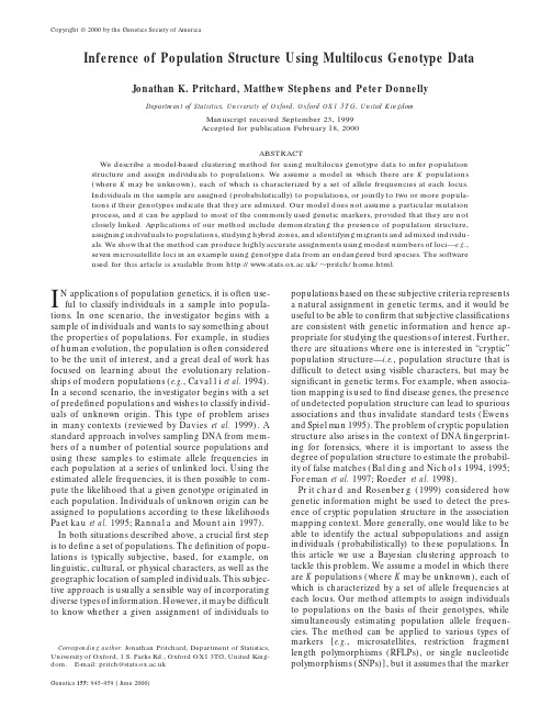
Copyright©2000by the Genetics Society of AmericaInference of Population Structure Using Multilocus Genotype DataJonathan K.Pritchard,Matthew Stephens and Peter DonnellyDepartment of Statistics,University of Oxford,Oxford OX13TG,United KingdomManuscript received September23,1999Accepted for publication February18,2000ABSTRACTWe describe a model-based clustering method for using multilocus genotype data to infer populationstructure and assign individuals to populations.We assume a model in which there are K populations(where K may be unknown),each of which is characterized by a set of allele frequencies at each locus.Individuals in the sample are assigned(probabilistically)to populations,or jointly to two or more popula-tions if their genotypes indicate that they are admixed.Our model does not assume a particular mutationprocess,and it can be applied to most of the commonly used genetic markers,provided that they are notclosely linked.Applications of our method include demonstrating the presence of population structure,assigning individuals to populations,studying hybrid zones,and identifying migrants and admixed individu-als.We show that the method can produce highly accurate assignments using modest numbers of loci—e.g.,seven microsatellite loci in an example using genotype data from an endangered bird species.The softwareused for this article is available from /فpritch/home.html.I N applications of population genetics,it is often use-populations based on these subjective criteria representsa natural assignment in genetic terms,and it would beful to classify individuals in a sample into popula-tions.In one scenario,the investigator begins with a useful to be able to conﬁrm that subjective classiﬁcations sample of individuals and wants to say something aboutare consistent with genetic information and hence ap-the properties of populations.For example,in studies propriate for studying the questions of interest.Further, of human evolution,the population is often consideredthere are situations where one is interested in“cryptic”to be the unit of interest,and a great deal of work has population structure—i.e.,population structure that isdifﬁcult to detect using visible characters,but may be focused on learning about the evolutionary relation-ships of modern populations(e.g.,Cavalli et al.1994).signiﬁcant in genetic terms.For example,when associa-In a second scenario,the investigator begins with a settion mapping is used toﬁnd disease genes,the presence of predeﬁned populations and wishes to classify individ-of undetected population structure can lead to spurious uals of unknown origin.This type of problem arisesassociations and thus invalidate standard tests(Ewens in many contexts(reviewed by Davies et al.1999).A and Spielman1995).The problem of cryptic population standard approach involves sampling DNA from mem-structure also arises in the context of DNAﬁngerprint-bers of a number of potential source populations and ing for forensics,where it is important to assess thedegree of population structure to estimate the probabil-using these samples to estimate allele frequencies inity of false matches(Balding and Nichols1994,1995; each population at a series of unlinked ing theForeman et al.1997;Roeder et al.1998).estimated allele frequencies,it is then possible to com-Pritchard and Rosenberg(1999)considered how pute the likelihood that a given genotype originated ingenetic information might be used to detect the pres-each population.Individuals of unknown origin can beence of cryptic population structure in the association assigned to populations according to these likelihoodsmapping context.More generally,one would like to be Paetkau et al.1995;Rannala and Mountain1997).able to identify the actual subpopulations and assign In both situations described above,a crucialﬁrst stepindividuals(probabilistically)to these populations.In is to deﬁne a set of populations.The deﬁnition of popu-this article we use a Bayesian clustering approach to lations is typically subjective,based,for example,ontackle this problem.We assume a model in which there linguistic,cultural,or physical characters,as well as theare K populations(where K may be unknown),each of geographic location of sampled individuals.This subjec-which is characterized by a set of allele frequencies at tive approach is usually a sensible way of incorporatingeach locus.Our method attempts to assign individuals diverse types of information.However,it may be difﬁcultto populations on the basis of their genotypes,while to know whether a given assignment of individuals tosimultaneously estimating population allele frequen-cies.The method can be applied to various types ofmarkers[e.g.,microsatellites,restriction fragment Corresponding author:Jonathan Pritchard,Department of Statistics,length polymorphisms(RFLPs),or single nucleotide University of Oxford,1S.Parks Rd.,Oxford OX13TG,United King-dom.E-mail:pritch@ polymorphisms(SNPs)],but it assumes that the marker Genetics155:945–959(June2000)946J.K.Pritchard,M.Stephens and P.Donnellyloci are unlinked and at linkage equilibrium with one observations from each cluster are random draws another within populations.It also assumes Hardy-Wein-from some parametric model.Inference for the pa-berg equilibrium within populations.(We discuss these rameters corresponding to each cluster is then done assumptions further in background on clusteringjointly with inference for the cluster membership of methods and the discussion.)each individual,using standard statistical methods Our approach is reminiscent of that taken by Smouse(for example,maximum-likelihood or Bayesian et al.(1990),who used the EM algorithm to learn about methods).the contribution of different breeding populations to aDistance-based methods are usually easy to apply and sample of salmon collected in the open ocean.It is alsoare often visually appealing.In the genetics literature,it closely related to the methods of Foreman et al.(1997)has been common to adapt distance-based phylogenetic and Roeder et al.(1998),who were concerned withalgorithms,such as neighbor-joining,to clustering estimating the degree of cryptic population structuremultilocus genotype data(e.g.,Bowcock et al.1994). to assess the probability of obtaining a false match atHowever,these methods suffer from many disadvan-DNAﬁngerprint loci.Consequently they focused ontages:the clusters identiﬁed may be heavily dependent estimating the amount of genetic differentiation amongon both the distance measure and graphical representa-the unobserved populations.In contrast,our primarytion chosen;it is difﬁcult to assess how conﬁdent we interest lies in the assignment of individuals to popula-should be that the clusters obtained in this way are tions.Our approach also differs in that it allows for themeaningful;and it is difﬁcult to incorporate additional presence of admixed individuals in the sample,whoseinformation such as the geographic sampling locations genetic makeup is drawn from more than one of the Kof individuals.Distance-based methods are thus more populations.suited to exploratory data analysis than toﬁne statistical In the next section we provide a brief descriptioninference,and we have chosen to take a model-based of clustering methods in general and describe someapproach here.advantages of the model-based approach we take.TheTheﬁrst challenge when applying model-based meth-details of the models and algorithms used are given inods is to specify a suitable model for observations from models and methods.We illustrate our method witheach cluster.To make our discussion more concrete we several examples in applications to data:both onintroduce very brieﬂy some of our model and notation simulated data and on sets of genotype data from anhere;a fuller treatment is given later.Assume that each endangered bird species and from humans.incorpo-cluster(population)is modeled by a characteristic set rating population information describes how ourof allele frequencies.Let X denote the genotypes of the method can be extended to incorporate geographicsampled individuals,Z denote the(unknown)popula-information into the inference process.This may betions of origin of the individuals,and P denote the useful for testing whether particular individuals are mi-(unknown)allele frequencies in all populations.(Note grants or to assist in classifying individuals of unknownthat X,Z,and P actually represent multidimensional origin(as in Rannala and Mountain1997,for exam-vectors.)Our main modeling assumptions are Hardy-ple).Background on the computational methods usedWeinberg equilibrium within populations and complete in this article is provided in the appendix.linkage equilibrium between loci within populations.Under these assumptions each allele at each locus ineach genotype is an independent draw from the appro-BACKGROUND ON CLUSTERING METHODSpriate frequency distribution,and this completely speci-Consider a situation where we have genetic data fromﬁes the probability distribution Pr(X|Z,P)(given later a sample of individuals,each of whom is assumed toin Equation2).Loosely speaking,the idea here is that have originated from a single unknown population(nothe model accounts for the presence of Hardy-Weinberg admixture).Suppose we wish to cluster together individ-or linkage disequilibrium by introducing population uals who are genetically similar,identify distinct clusters,structure and attempts toﬁnd population groupings and perhaps see how these clusters relate to geographi-that(as far as possible)are not in disequilibrium.While cal or phenotypic data on the individuals.There areinference may depend heavily on these modeling as-broadly two types of clustering methods we might use:sumptions,we feel that it is easier to assess the validityof explicit modeling assumptions than to compare the 1.Distance-based methods.These proceed by calculatingrelative merits of more abstract quantities such as dis-a pairwise distance matrix,whose entries give thetance measures and graphical representations.In situa-distance(suitably deﬁned)between every pair of in-tions where these assumptions are deemed unreason-dividuals.This matrix may then be represented usingable then alternative models should be built.some convenient graphical representation(such as aHaving speciﬁed our model,we must decide how to tree or a multidimensional scaling plot)and clustersperform inference for the quantities of interest(Z and may be identiﬁed by eye.2.Model-based methods.These proceed by assuming that P).Here,we have chosen to adopt a Bayesian approach,947Inferring Population Structureby specifying models(priors)Pr(Z)and Pr(P),for both Assume that before observing the genotypes we haveZ and P.The Bayesian approach provides a coherent no information about the population of origin of eachframework for incorporating the inherent uncertainty individual and that the probability that individual i origi-of parameter estimates into the inference procedure nated in population k is the same for all k,and for evaluating the strength of evidence for the in-Pr(z(i)ϭk)ϭ1/K,(3) ferred clustering.It also eases the incorporation of vari-ous sorts of prior information that may be available,independently for all individuals.(In cases where somesuch as information about the geographic sampling lo-populations may be more heavily represented in thecation of individuals.sample than others,this assumption is inappropriate;itHaving observed the genotypes,X,our knowledge would be straightforward to extend our model to dealabout Z and P is then given by the posterior distribution with such situations.)We follow the suggestion of Balding and Nichols Pr(Z,P|X)ϰPr(Z)Pr(P)Pr(X|Z,P).(1)(1995)(see also Foreman et al.1997and Rannala While it is not usually possible to compute this distribu-and Mountain1997)in using the Dirichlet distri-tion exactly,it is possible to obtain an approximate bution to model the allele frequencies at each locus sample(Z(1),P(1)),(Z(2),P(2)),...,(Z(M),P(M))from Pr(Z,within each population.The Dirichlet distributionP|X)using Markov chain Monte Carlo(MCMC)meth-D(␭1,␭2,...,␭J)is a distribution on allele frequenciesods described below(see Gilks et al.1996b,for more pϭ(p1,p2,...,p J)with the property that these frequen-general background).Inference for Z and P may then cies sum to1.We use this distribution to specify the be based on summary statistics obtained from this sam-probability of a particular set of allele frequencies pkl·ple(see Inference for Z,P,and Q below).A brief introduc-for population k at locus l,tion to MCMC methods and Gibbs sampling may befound in the appendix.pkl·فD(␭1,␭2,...,␭J l),(4)independently for each k,l.The expected frequency of MODELS AND METHODS allele j is proportional to␭j,and the variance of thisfrequency decreases as the sum of the␭j increases.We We now provide a more detailed description of ourtake␭1ϭ␭2ϭ···ϭ␭J lϭ1.0,which gives a uniform modeling assumptions and the algorithms used to per-distribution on the allele frequencies;alternatives are form inference,beginning with the simpler case wherediscussed in the discussion.each individual is assumed to have originated in a singleMCMC algorithm(without admixture):Equations2, population(no admixture).3,and4deﬁne the quantities Pr(X|Z,P),Pr(Z),and The model without admixture:Suppose we genotypePr(P),respectively.By setting␪ϭ(␪1,␪2)ϭ(Z,P)and N diploid individuals at L loci.In the case without admix-letting␲(Z,P)ϭPr(Z,P|X)we can use the approach ture,each individual is assumed to originate in one ofoutlined in Algorithm A1to construct a Markov chain K populations,each with its own characteristic set ofwith stationary distribution Pr(Z,P|X)as follows: allele frequencies.Let the vector X denote the observedAlgorithm1:Starting with initial values Z(0)for Z(by genotypes,Z the(unknown)populations of origin ofdrawing Z(0)at random using(3)for example),iterate the the individuals,and P the(unknown)allele frequenciesfollowing steps for mϭ1,2,....in the populations.These vectors consist of the follow-ing elements,Step1.Sample P(m)from Pr(P|X,Z(mϪ1)).(x(i,1)l,x(i,2)l)ϭgenotype of the i th individual at the l th locus,Step2.Sample Z(m)from Pr(Z|X,P(m)).where iϭ1,2,...,N and lϭ1,2,...,L;z(i)ϭpopulation from which individual i originated;Informally,step1corresponds to estimating the allele p kljϭfrequency of allele j at locus l in population k,frequencies for each population assuming that the pop-where kϭ1,2,...,K and jϭ1,2,...,J l,ulation of origin of each individual is known;step2 where J l is the number of distinct alleles observed at corresponds to estimating the population of origin of locus l,and these alleles are labeled1,2,...,J l.each individual,assuming that the population allele fre-Given the population of origin of each individual,quencies are known.For sufﬁciently large m and c,(Z(m), the genotypes are assumed to be generated by drawing P(m)),(Z(mϩc),P(mϩc)),(Z(mϩ2c),P(mϩ2c)),...will be approxi-alleles independently from the appropriate population mately independent random samples from Pr(Z,P|X). frequency distributions,The distributions required to perform each step aregiven in the appendix.Pr(x(i,a)lϭj|Z,P)ϭp z(i)lj(2)The model with admixture:We now expand ourmodel to allow for admixed individuals by introducing independently for each x(i,a)l.(Note that p z(i)lj is the fre-a vector Q to denote the admixture proportions for each quency of allele j at locus l in the population of originof individual i.)individual.The elements of Q are948J.K.Pritchard,M.Stephens and P.Donnellyq (i )k ϭproportion of individual i ’s genome thattion of origin of each allele copy in each individual isknown;step 2corresponds to estimating the population originated from population k.of origin of each allele copy,assuming that the popula-It is also necessary to modify the vector Z to replace the tion allele frequencies and the admixture proportions assumption that each individual i originated in some are known.As before,for sufﬁciently large m and c ,unknown population z (i )with the assumption that each (Z (m ),P (m ),Q (m )),(Z (m ϩc ),P (m ϩc ),Q (m ϩc )),(Z (m ϩ2c ),P (m ϩ2c ),observed allele copy x (i ,a )l originated in some unknown Q (m ϩ2c )),...will be approximately independent random population z (i ,a )l :samples from Pr(Z ,P ,Q |X ).The distributions required to perform each step are given in the appendix.z (i ,a )l ϭpopulation of origin of allele copy x (i ,a )l .Inference:Inference for Z,P,and Q:We now discuss how We use the term “allele copy”to refer to an allele carried the MCMC output can be used to perform inference on at a particular locus by a particular individual.Z ,P ,and Q.For simplicity,we focus our attention on Q ;Our primary interest now lies in estimating Q.We inference for Z or P is similar.proceed in a manner similar to the case without admix-Having obtained a sample Q (1),...,Q (M )(using suitably ture,beginning by specifying a probability model for large burn-in m and thinning interval c )from the poste-(X ,Z ,P ,Q ).Analogues of (2)and (3)arerior distribution of Q ϭ(q 1,...,q N )given X using the MCMC method,it is desirable to summarize the Pr(x (i ,a )l ϭj |Z ,P ,Q )ϭp z (i ,a )l lj(5)information contained,perhaps by a point estimate of andQ.A seemingly obvious estimate is the posterior meanPr(z (i ,a )l ϭk |P ,Q )ϭq (i )k ,(6)E (q i |X )≈1M ͚M m ϭ1q (m )i .(8)with (4)being used to model P as before.To complete our model we need to specify a distribution for Q ,which However,the symmetry of our model implies that the in general will depend on the type and amount of admix-posterior mean of q i is (1/K ,1/K ,...,1/K )for all i ,ture we expect to see.Here we model the admixturewhatever the value of X.For example,suppose that there proportions q (i )ϭ(q (i )1,...,q (i )K )of individual i using are just two populations and 10individuals and that the the Dirichlet distributiongenotypes of these individuals contain strong informa-tion that the ﬁrst 5are in one population and the second q (i )فD (␣,␣,...,␣)(7)5are in the other population.Then eitherindependently for each individual.For large values of ␣(ӷ1),this models each individual as having allele q 1...q 5≈(1,0)and q 6...q 10≈(0,1)(9)copies originating from all K populations in equal pro-orportions.For very small values of ␣(Ӷ1),it models each individual as originating mostly from a single popu-q 1...q 5≈(0,1)and q 6...q 10≈(1,0),(10)lation,with each population being equally likely.As with these two “symmetric modes”being equally likely,␣→0this model becomes the same as our model leading to the expectation of any given q i being (0.5,without admixture (although the implementation of the 0.5).This is essentially a problem of nonidentiﬁability MCMC algorithm is somewhat different).We allow ␣caused by the symmetry of the model [see Stephens to range from 0.0to 10.0and attempt to learn about ␣(2000b)for more discussion].from the data (speciﬁcally we put a uniform prior on In general,if there are K populations then there will ␣෈[0,10]and use a Metropolis-Hastings update step be K !sets of symmetric modes.Typically,MCMC to integrate out our uncertainty in ␣).This model may schemes ﬁnd it rather difﬁcult to move between such be considered suitable for situations where little is modes,and the algorithms we describe will usually ex-known about admixture;alternatives are discussed in plore only one of the symmetric modes,even when run the discussion.for a very large number of iterations.Fortunately this MCMC algorithm (with admixture):The following does not bother us greatly,since from the point of algorithm may be used to sample from Pr(Z ,P ,Q |X ).view of clustering all the symmetric modes are the same Algorithm 2:Starting with initial values Z (0)for Z (by drawing Z (0)at random using (3)for example),iterate the [compare the clusterings corresponding to (9)and following steps for m ϭ1,2,....(10)].If our sampler explores only one symmetric mode then the sample means (8)will be very poor estimates Step 1.Sample P (m ),Q (m )from Pr(P ,Q |X ,Z (m Ϫ1)).of the posterior means for the q i ,but will be much better Step 2.Sample Z (m )from Pr(Z |X ,P (m ),Q (m )).estimates of the modes of the q i ,which in this case turn Step 3.Update ␣using a Metropolis-Hastings step.out to be a much better summary of the information in the data.Ironically then,the poor mixing of the Informally,step 1corresponds to estimating the allele MCMC sampler between the symmetric modes gives frequencies for each population and the admixture pro-portions of each individual,assuming that the popula-the asymptotically useless estimator (8)some practical949Inferring Population Structure value.Where the MCMC sampler succeeds in moving Simulated data:To test the performance of the clus-tering method in cases where the “answers”are known,between symmetric modes,or where it is desired to combine results from samples obtained using different we simulated data from three population models,using standard coalescent techniques (Hudson 1990).We as-starting points (which may involve combining results corresponding to different modes),more sophisticated sumed that sampled individuals were genotyped at a series of unlinked microsatellite loci.Data were simu-methods [such as those described by Stephens (2000b)]may be required.lated under the following models.Inference for the number of populations:The problem of Model 1:A single random-mating population of con-inferring the number of clusters,K ,present in a data stant size.set is notoriously difﬁcult.In the Bayesian paradigm the Model 2:Two random-mating populations of constant way to proceed is theoretically straightforward:place a effective population size 2N.These were assumed to prior distribution on K and base inference for K on the have split from a single ancestral population,also of posterior distributionsize 2N at a time N generations in the past,with no subsequent migration.Pr(K |X )ϰPr(X |K )Pr(K ).(11)Model 3:Admixture of populations.Two discrete popu-However,this posterior distribution can be peculiarly lations of equal size,related as in model 2,were fused dependent on the modeling assumptions made,even to produce a single random-mating population.Sam-where the posterior distributions of other quantities (Q ,ples were collected after two generations of random Z ,and P ,say)are relatively robust to these assumptions.mating in the merged population.Thus,individuals Moreover,there are typically severe computational chal-have i grandparents from population 1,and 4Ϫi lenges in estimating Pr(X |K ).We therefore describe an grandparents from population 2with probability alternative approach,which is motivated by approximat-(4i )/16,where i ෈{0,4}.All loci were simulated inde-ing (11)in an ad hoc and computationally convenient pendently.way.We present results from analyzing data sets simulated Arguments given in the appendix (Inference on K,the under each model.Data set 1was simulated under number of populations )suggest estimating Pr(X |K )usingmodel 1,with 5microsatellite loci.Data sets 2A and 2B Pr(X |K )≈exp(Ϫ␮ˆ/2Ϫ␴ˆ2/8),(12)were simulated under model 2,with 5and 15microsatel-lite loci,respectively.Data set 3was simulated under wheremodel 3,with 60loci (preliminary analyses with fewer loci showed this to be a much harder problem than ␮ˆϭ1M ͚M m ϭ1Ϫ2log Pr(X |Z (m ),P (m ),Q (m ))(13)models 1and 2).Microsatellite mutation was modeled by a simple stepwise mutation process,with the mutation andparameter 4N ␮set at 16.0per locus (i.e.,the expected variance in repeat scores within populations was 8.0).␴ˆ2ϭ1M ͚Mm ϭ1(Ϫ2log Pr(X |Z (m ),P (m ),Q (m ))Ϫ␮ˆ)2.We did not make use of the assumed mutation model in analyzing the simulated data.(14)Our analysis consists of two phases.First,we consider We use (12)to estimate Pr(X |K )for each K and substi-the issue of model choice—i.e.,how many populations tute these estimates into (11)to approximate the poste-are most appropriate for interpreting the data.Then,rior distribution Pr(K |X ).we examine the clustering of individuals for the inferred In fact,the assumptions underlying (12)are dubious number of populations.at best,and we do not claim (or believe)that our proce-Choice of K for simulated data:For each model,we dure provides a quantitatively accurate estimate of the ran a series of independent runs of the Gibbs sampler posterior distribution of K.We see it merely as an ad for each value of K (the number of populations)be-hoc guide to which models are most consistent with the tween 1and 5.The results presented are based on runs data,with the main justiﬁcation being that it seems of 106iterations or more,following a burn-in period of to give sensible answers in practice (see next section for at least 30,000iterations.To choose the length of the examples).Notwithstanding this,for convenience we burn-in period,we printed out log(Pr(X |P (m ),Q (m ))),and continue to refer to “estimating”Pr(K |X )and Pr(X |K ).several other summary statistics during the course of a series of trial runs,to estimate how long it took to reach (approximate)stationarity.To check for possible prob-APPLICATIONS TO DATAlems with mixing,we compared the estimates of P (X |K )and other summary statistics obtained over several inde-We now illustrate the performance of our method on both simulated data and real data (from an endangered pendent runs of the Gibbs sampler,starting from differ-ent initial points.In general,substantial differences be-bird species and from humans).The analyses make use of the methods described in The model with admixture.tween runs can indicate that either the runs should950J.K.Pritchard,M.Stephens and P.DonnellyTABLE 1Estimated posterior probabilities of K ,for simulated data sets 1,2A,2B,and 3(denoted X 1,X 2A ,X 2B ,and X 3,respectively)K log P (K |X 1)P (K |X 2A )P (K |X 2B )P (K |X 3)1ف1.0ف0.0ف0.0ف0.02ف0.00.210.999ف1.03ف0.00.580.0009ف0.04ف0.00.21ف0.0ف0.05ف0.0ف0.0ف0.0ف0.0The numbers should be regarded as a rough guide to which models are consistent with the data,rather than accurate esti-mates of posterior probabilities.Figure 1.—Summary of the clustering results for simulated data sets 2A and 2B,respectively.For each individual,webe longer to obtain more accurate estimates or that computed the mean value of q (i )1(the proportion of ancestry independent runs are getting stuck in different modes in population 1),over a single run of the Gibbs sampler.Thein the parameter space.(Here,we consider the K !dashed line is a histogram of mean values of q (i )1for individuals from population 0;the solid line is for individuals from popula-modes that arise from the nonidentiﬁability of the K tion 1.populations to be equivalent,since they arise from per-muting the K population labels.)We found that in most cases we obtained consistent and Q estimating the number of grandparents from estimates of P (X |K )across independent runs.However,each of the two original populations,for each individual.when analyzing data set 2A with K ϭ3,the Gibbs sampler Intuitively it seems that another plausible clustering found two different modes.This data set actually con-would be with K ϭ5,individuals being assigned to tains two populations,and when K is set to 3,one of clusters according to how many grandparents they have the populations expands to ﬁll two of the three clusters.from each population.In biological terms,the solution It is somewhat arbitrary which of the two populations with K ϭ2is more natural and is indeed the inferred expands to ﬁll the extra cluster:this leads to two modes value of K for this data set using our ad hoc guide [the of slightly different heights.The Gibbs sampler did not estimated value of Pr(X |K )was higher for K ϭ5than manage to move between the two modes in any of our for K ϭ3,4,or 6,but much lower than for K ϭ2].runs.However,this raises an important point:the inferred In Table 1we report estimates of the posterior proba-value of K may not always have a clear biological inter-bilities of values of K ,assuming a uniform prior on K pretation (an issue that we return to in the discussion ).between 1and 5,obtained as described in Inference for Clustering of simulated data:Having considered the the number of populations.We repeat the warning given problem of estimating the number of populations,we there that these numbers should be regarded as rough now examine the performance of the clustering algo-guides to which models are consistent with the data,rithm in assigning particular individuals to the appro-rather than accurate estimates of the posterior probabil-priate populations.In the case where the populations ities.In the case where we found two modes (data set are discrete,the clustering performs very well (Figure 2A,K ϭ3),we present results based on the mode that 1),even with just 5loci (data set 2A),and essentially gave the higher estimate of Pr(X |K ).perfectly with 15loci (data set 2B).With all four simulated data sets we were able to The case with admixture (Figure 2)appears to be correctly infer whether or not there was population more difﬁcult,even using many more loci.However,structure (K ϭ1for data set 1and K Ͼ1otherwise).the clustering algorithm did manage to identify the In the case of data set 2A,which consisted of just 5population structure appropriately and estimated the loci,there is not a clear estimate of K ,as the posterior ancestry of individuals with reasonable accuracy.Part probability is consistent with both the correct value,K ϭof the reason that this problem is difﬁcult is that it is 2,and also with K ϭ3or 4.However,when the number hard to estimate the original allele frequencies (before of loci was increased to 15(data set 2B),virtually all of admixture)when almost all the individuals (7/8)are the posterior probability was on the correct number of admixed.A more fundamental problem is that it is difﬁ-populations,K ϭ2.cult to get accurate estimates of q (i )for particular individ-Data set 3was simulated under a more complicated uals because (as can be seen from the y -axis of Figure model,where most individuals have mixed ancestry.In 2)for any given individual,the variance of how many this case,the population was formed by admixture of two populations,so the “true”clustering is with K ϭ2,of its alleles are actually derived from each population。

地特胰岛素联合门冬胰岛素治疗妊娠期糖尿病疗效与安全性及对母婴结局的影响研究

DOI：10.16658/ki.1672-4062.2023.18.113地特胰岛素联合门冬胰岛素治疗妊娠期糖尿病疗效与安全性及对母婴结局的影响研究王霞平遥县人民医院产科，山西晋中031100[摘要]目的探讨妊娠期糖尿病（gestational diabetes mellitus, GDM）产妇应用地特胰岛素联合门冬胰岛素治疗的效果。

方法选取2021年7月—2022年9月期间在平遥县人民医院进行分娩的GDM产妇66例为研究对象，按隐匿数字随机法分为单药组（33例，门冬胰岛素治疗），联合组（33例，门冬胰岛素+地特胰岛素治疗），观察记录两组血糖变化、胰岛素水平、母婴结局，进行比较分析。

结果治疗前，两组患者血糖控制水平比较，差异无统计学意义（P>0.05）；治疗后，联合组的空腹血糖（fasting plasma glucose, FPG）、餐后2 h血糖（2-hourpostprandial blood glucose，2 hPG）、糖化血红蛋白（glycated hemoglobin, HbA1c）水平均低于单药组，差异有统计学意义（P<0.05）；联合组的FPG达标、2 hFPG达标、FPG和2 hFPG均达标的时间均显著短于单药组，差异有统计学意义（P<0.05）；联合组的自然分娩率为72.73%显著高于单药组的48.48%，差异有统计学意义（P< 0.05）；单药组的不良妊娠结局发生率（24.24%）高于联合组（9.09%），差异无统计学意义（P>0.05）。

结论地特胰岛素联合门冬胰岛素治疗GDM患者，可以获得较为理想的血糖控制效果，能更快的使患者血糖达到理想的标准，自然分娩率更高。

[关键词] 妊娠期糖尿病；地特胰岛素；门冬胰岛素；母婴结局[中图分类号] R714 [文献标识码] A [文章编号] 1672-4062（2023）09（b）-0113-04Study on the Efficacy and Safety of Insulin Detemir Combined with Insu⁃lin Aspart in the Treatment of Gestational Diabetes and Its Impact on Ma⁃ternal and Fetal OutcomesWANG XiaDepartment of Obstetrics, Pingyao County People's Hospital, Jinzhong, Shanxi Province, 031100 China[Abstract] Objective To explore the effect of insulin detemir combined with insulin aspart in the treatment of gesta‐tional diabetes mellitus (GDM). Methods 66 GDM women who gave birth in Pingyao County People's Hospital from July 2021 to September 2022 were selected as research objects. According to the concealed number random method, 33 patients were divided into a single-drug group (treated with insulin aspart) and 33 patients were combination group (treated with insulin aspart+insulin detemir). Observed and recorded the data on blood sugar changes, insulin levels, and maternal and infant outcomes between the two groups for comparative analysis. Results Before treatment, there was no statistically significant difference in blood glucose control levels between the two groups (P>0.05). After treat‐ment, the levels of fasting plasma glucose (FPG), 2-hour postprandial blood glucose (2 hPG), and glycated hemoglobin (HbA1c) in the combination group were lower than those in the single-drug group, the difference was statistically sig‐nificant (P<0.05). The time for FPG to reach the target, 2 hPG to reach the target, and both FPG and 2 hPG to reach the target in the combination group were significantly shorter than those in the single-drug group, the difference were statistically significant (P<0.05). The natural delivery rate in the combination group was 72.73%, which was signifi‐cantly higher than the 48.48% in the single-drug group, the difference was statistically significant (P<0.05). The inci‐dence rate of adverse pregnancy outcomes in the single-drug group (24.24%) was higher than that in the combination group (9.09%), and the difference was statistically significant (P>0.05). Conclusion Insulin detemir combined with in‐sulin aspart can achieve ideal blood sugar control effects in patients with GDM, and can bring patients' blood sugar to the ideal standard faster, and the natural delivery rate is higher.[作者简介]王霞（1979-），女，本科，副主任医师，研究方向为产科及相关疾病诊治。

多变量核密度估计与Vine复杂体（kdevine包）v0.4.4用户指南说明书

Package‘kdevine’October18,2022Type PackageTitle Multivariate Kernel Density Estimation with Vine CopulasVersion0.4.4URL https:///tnagler/kdevineBugReports https:///tnagler/kdevine/issuesDescription Implements the vine copula based kernel density estimator ofNagler and Czado(2016)<doi:10.1016/j.jmva.2016.07.003>.The estimator doesnot suffer from the curse of dimensionality and is therefore well suited forhigh-dimensional applications.License GPL-3Imports graphics,stats,utils,MASS,Rcpp,qrng,KernSmooth,cctools,kdecopula(>=0.8.1),VineCopula,doParallel,parallel,foreachLazyData yesLinkingTo RcppRoxygenNote7.2.0Suggests testthatNeedsCompilation yesAuthor Thomas Nagler[aut,cre]Maintainer Thomas Nagler<****************>Repository CRANDate/Publication2022-10-1812:25:15UTCR topics documented:kdevine-package (2)contour.kdevinecop (3)dkde1d (3)dkdevine (4)dkdevinecop (5)kde1d (6)12kdevine-package kdevine (7)kdevinecop (9)plot.kde1d (10)rkdevine (11)wdbc (12)Index14 kdevine-package Kernel Smoothing for Bivariate Copula DensitiesDescriptionThis package implements a vine copula based kernel density estimator.The estimator does not suf-fer from the curse of dimensionality and is therefore well suited for high-dimensional applications (see,Nagler and Czado,2016).DetailsThe multivariate kernel density estimators is implemented by the kdevine function.It combines a kernel density estimator for the margins(kde1d)and a kernel estimator of the vine copula density (kdevinecop).The package is built on top of the copula density estimators in the kdecopula::kdecopula-package and let’s you choose from all its implemented methods.Optionally,the vine copula can be estimated parameterically(only the margins are nonparametric).Author(s)Thomas NaglerReferencesNagler,T.,Czado,C.(2016)Evading the curse of dimensionality in nonparametric density estimation with simpliﬁed vine copu-las.Journal of Multivariate Analysis151,69-89(doi:10.1016/j.jmva.2016.07.003)Nagler,T.,Schellhase,C.and Czado,C.(2017)Nonparametric estimation of simpliﬁed vine copula models:comparison of methods arXiv:1701.00845 Nagler,T.(2017)A generic approach to nonparametric function estimation with mixed data.arXiv:1704.07457contour.kdevinecop3 contour.kdevinecop Contour plots of pair copula kernel estimatesDescriptionContour plots of pair copula kernel estimatesUsage##S3method for class kdevinecopcontour(x,tree="ALL",xylim=NULL,cex.nums=1,...)Argumentsx a kdevinecop object.tree"ALL"or integer vector;speciﬁes which trees are plotted.xylim numeric vector of length2;sets xlim and ylim for the contours.cex.nums numeric;expansion factor for font of the numbers....arguments passed to contour.kdecopula.Examplesdata(wdbc,package="kdecopula")#load datau<-VineCopula::pobs(wdbc[,5:7],ties="average")#rank-transform#estimate densityfit<-kdevinecop(u)#contour matrixcontour(fit)dkde1d Working with a kde1d objectDescriptionThe density,cdf,or quantile function of a kernel density estimate are evaluated at arbitrary points with dkde1d,pkde1d,and qkde1d respectively.4dkdevineUsagedkde1d(x,obj)pkde1d(x,obj)qkde1d(x,obj)rkde1d(n,obj,quasi=FALSE)Argumentsx vector of evaluation points.obj a kde1d object.n integer;number of observations.quasi logical;the default(FALSE)returns pseudo-random numbers,use TRUE for quasi-random numbers(generalized Halton,see ghalton).ValueThe density or cdf estimate evaluated at x.See Alsokde1dExamplesdata(wdbc)#load datafit<-kde1d(wdbc[,5])#estimate densitydkde1d(1000,fit)#evaluate density estimatepkde1d(1000,fit)#evaluate corresponding cdfqkde1d(0.5,fit)#quantile functionhist(rkde1d(100,fit))#simulatedkdevine Evaluate the density of a kdevine objectDescriptionEvaluate the density of a kdevine objectUsagedkdevine(x,obj)dkdevinecop5Argumentsx(mxd)matrix of evaluation points(or vector of length d).obj a kdevine object.ValueThe density estimate evaluated at x.See AlsokdevineExamples#load datadata(wdbc)#estimate density(use xmin to indicate positive support)fit<-kdevine(wdbc[,5:7],xmin=rep(0,3))#evaluate density estimatedkdevine(c(1000,0.1,0.1),fit)dkdevinecop Working with a kdevinecop objectDescriptionA vine copula density estimate(stored in a kdevinecop object)can be evaluated on arbitrary pointswith dkevinecop.Furthermore,you can simulate from the estimated density with rkdevinecop. Usagedkdevinecop(u,obj,stable=FALSE)rkdevinecop(n,obj,U=NULL,quasi=FALSE)Argumentsu mx2matrix of evaluation points.obj kdevinecop object.stable logical;option for stabilizing the estimator:the estimated pair copula density is cut off at50.n integer;number of observations.U(optional)nxd matrix of independent uniform random variables.quasi logical;the default(FALSE)returns pseudo-random numbers,use TRUE for quasi-random numbers(generalized Halton,see ghalton).6kde1d ValueA numeric vector of the density/cdf or a nx2matrix of simulated data.Author(s)Thomas NaglerReferencesNagler,T.,Czado,C.(2016)Evading the curse of dimensionality in nonparametric density estimation.Journal of Multivariate Analysis151,69-89(doi:10.1016/j.jmva.2016.07.003)Dissmann,J.,Brechmann,E.C.,Czado,C.,and Kurowicka,D.(2013).Selecting and estimating regular vine copulae and application toﬁnancial returns.Computational Statistics&Data Analysis,59(0):52–69.See Alsokdevinecop,dkdecop,rkdecop,ghaltonExamplesdata(wdbc,package="kdecopula")#load datau<-VineCopula::pobs(wdbc[,5:7],ties="average")#rank-transformfit<-kdevinecop(u)#estimate densitydkdevinecop(c(0.1,0.1,0.1),fit)#evaluate density estimatekde1d Univariate kernel density estimation for bounded and unbounded sup-portDescriptionDiscrete variables are convoluted with the uniform distribution(see,Nagler,2017).If a variable should be treated as discrete,declare it as ordered().Usagekde1d(x,mult=1,xmin=-Inf,xmax=Inf,bw=NULL,bw_min=0,...)Argumentsx vector of length n.mult numeric;the actual bandwidth used is bw∗mult.xmin lower bound for the support of the density.xmax upper bound for the support of the density.bw bandwidth parameter;has to be a positive number or NULL;the latter calls KernSmooth::dpik().bw_min minimum value for the bandwidth....unused.DetailsIf xmin or xmax areﬁnite,the density estimate will be0outside of[xmin,xmax].Mirror-reﬂectionis used to correct for boundary bias.Discrete variables are convoluted with the uniform distribution(see,Nagler,2017).ValueAn object of class kde1d.ReferencesNagler,T.(2017).A generic approach to nonparametric function estimation with mixed data.arXiv:1704.07457See Alsodkde1d,pkde1d,qkde1d,rkde1d plot.kde1d,lines.kde1dExamplesdata(wdbc,package="kdecopula")#load datafit<-kde1d(wdbc[,5])#estimate densitydkde1d(1000,fit)#evaluate density estimatekdevine Kernel density estimatior based on simpliﬁed vine copulasDescriptionImplements the vine-copula based estimator of Nagler and Czado(2016).The marginal densitiesare estimated by kde1d,the vine copula density by kdevinecop.Discrete variables are convolutedwith the uniform distribution(see,Nagler,2017).If a variable should be treated as discrete,declareit as ordered().Factors are expanded into binary dummy codes.Usagekdevine(x,mult_1d=NULL,xmin=NULL,xmax=NULL,copula.type="kde",...)Argumentsx(nxd)data matrix.mult_1d numeric;all bandwidhts for marginal kernel density estimation are multipliedwith mult_1d.Defaults to log(1+d)where d is the number of variables afterapplying cctools::expand_as_numeric().xmin numeric vector of length d;see kde1d.xmax numeric vector of length d;see kde1d.copula.type either"kde"(default)or"parametric"for kernel or parametric estimation ofthe vine copula....further arguments passed to kde1d or kdevinecop.ValueAn object of class kdevine.ReferencesNagler,T.,Czado,C.(2016)Evading the curse of dimensionality in nonparametric density estima-tion with simpliﬁed vine copulas.Journal of Multivariate Analysis151,69-89(doi:10.1016/j.jmva.2016.07.003)Nagler,T.(2017).A generic approach to nonparametric function estimation with mixed data.arXiv:1704.07457See Alsodkdevine kde1d kdevinecopExamples#load datadata(wdbc,package="kdecopula")#estimate density(use xmin to indicate positive support)fit<-kdevine(wdbc[,5:7],xmin=rep(0,3))#evaluate density estimatedkdevine(c(1000,0.1,0.1),fit)#plot simulated datapairs(rkdevine(nrow(wdbc),fit))kdevinecop9 kdevinecop Kernel estimation of vine copula densitiesDescriptionThe function estimates a vine copula density using kernel estimators for the pair copulas(based on the kdecopula package).Usagekdevinecop(data,matrix=NA,method="TLL2",renorm.iter=3L,mult=1,test.level=NA,trunc.level=NA,treecrit="tau",cores=1,info=FALSE)Argumentsdata(nxd)matrix of copula data(have to lie in[0,1d]).matrix R-Vine matrix(nxd)specifying the structure of the vine;if NA(default)thestructure selection heuristic of Dissman et al.(2013)is applied.method see kdecop.renorm.iter see kdecop.mult see kdecop.test.level signiﬁcance level for independence test.If you provide a number in[0,1],anindependence test(BiCopIndTest)will be performed for each pair;if the nullhypothesis of independence cannot be rejected,the independence copula willbe set for this pair.If test.level=NA(default),no independence test will beperformed.trunc.level integer;the truncation level.All pair copulas in trees above the truncation levelwill be set to independence.treecrit criterion for structure selection;defaults to"tau".cores integer;if cores>1,estimation will be parallized within each tree(using foreach).info logical;if TRUE,additional information about the estimate will be gathered(seekdecop).10plot.kde1dValueAn object of class kdevinecop.That is,a list containingT1,T2,...lists of the estimted pair copulas in each tree,matrix the structure matrix of the vine,info additional information about theﬁt(if info=TRUE).ReferencesNagler,T.,Czado,C.(2016)Evading the curse of dimensionality in nonparametric density estimation with simpliﬁed vine cop-ulas.Journal of Multivariate Analysis151,69-89(doi:10.1016/j.jmva.2016.07.003)Nagler,T.,Schellhase,C.and Czado,C.(2017)Nonparametric estimation of simpliﬁed vine copula models:comparison of methods arXiv:1701.00845 Dissmann,J.,Brechmann,E.C.,Czado,C.,and Kurowicka,D.(2013).Selecting and estimating regular vine copulae and application toﬁnancial returns.Computational Statistics&Data Analysis,59(0):52–69.See Alsodkdevinecop,kdecop,BiCopIndTest,foreachExamplesdata(wdbc,package="kdecopula")#rank-transform to copula data(margins are uniform)u<-VineCopula::pobs(wdbc[,5:7],ties="average")fit<-kdevinecop(u)#estimate densitydkdevinecop(c(0.1,0.1,0.1),fit)#evaluate density estimatecontour(fit)#contour matrix(Gaussian scale)pairs(rkdevinecop(500,fit))#plot simulated dataplot.kde1d Plotting kde1d objectsDescriptionPlotting kde1d objectsUsage##S3method for class kde1dplot(x,...)##S3method for class kde1dlines(x,...)rkdevine11Argumentsx kde1d object....further arguments passed to plot.default.See Alsokde1d lines.kde1dExamplesdata(wdbc)#load datafit<-kde1d(wdbc[,7])#estimate densityplot(fit)#plot density estimatefit2<-kde1d(as.ordered(wdbc[,1]))#discrete variableplot(fit2,col=2)rkdevine Simulate from a kdevine objectDescriptionSimulate from a kdevine objectUsagerkdevine(n,obj,quasi=FALSE)Argumentsn number of observations.obj a kdevine object.quasi logical;the default(FALSE)returns pseudo-random numbers,use TRUE for quasi-random numbers(generalized Halton,only works for fully nonparametricﬁts).ValueAn nxd matrix of simulated data from the kdevine object.See Alsokdevine,rkdevinecop,rkde1d12wdbcExamples#load and plot datadata(wdbc)#estimate densityfit<-kdevine(wdbc[,5:7],xmin=rep(0,3))#plot simulated datapairs(rkdevine(nrow(wdbc),fit))wdbc Wisconsin Diagnostic Breast Cancer(WDBC)DescriptionThe data contain measurements on cells in suspicious lumps in a women’s breast.Features are computed from a digitized image of aﬁne needle aspirate(FNA)of a breast mass.They describe characteristics of the cell nuclei present in the image.All samples are classsiﬁed as either benign or malignant.Usagedata(wdbc)Formatwdbc is a data.frame with31columns.Theﬁrst column indicates wether the sample is classiﬁed as benign(B)or malignant(M).The remaining columns contain measurements for30features.DetailsTen real-valued features are computed for each cell nucleus:a)radius(mean of distances from center to points on the perimeter)b)texture(standard deviation of gray-scale values)c)perimeterd)areae)smoothness(local variation in radius lengths)f)compactness(perimeter^2/area-1.0)g)concavity(severity of concave portions of the contour)h)concave points(number of concave portions of the contour)i)symmetryj)fractal dimension("coastline approximation"-1)The references listed below contain detailed descriptions of how these features are computed.The mean,standard error,and"worst"or largest(mean of the three largest values)of these features were computed for each image,resulting in30features.wdbc13NoteThis breast cancer database was obtained from the University of Wisconsin Hospitals,Madison from Dr.William H.Wolberg.Sourcehttps:///ml/datasets/Breast+Cancer+Wisconsin+(Diagnostic)Bache,K.&Lichman,M.(2013).UCI Machine Learning Repository.Irvine,CA:University of California,School of Information and Computer Science.ReferencesO.L.Mangasarian and W.H.Wolberg:"Cancer diagnosis via linear programming",SIAM News,V olume23,Number5,September1990,pp1&18.William H.Wolberg and O.L.Mangasarian:"Multisurface method of pattern separation for medical diagnosis applied to breast cytology",Proceedings of the National Academy of Sciences,U.S.A.,V olume87,December1990,pp9193-9196.K.P.Bennett&O.L.Mangasarian:"Robust linear programming discrimination of two linearly inseparable sets",Optimization Methods and Software1,1992,23-34(Gordon&Breach Science Publishers).Examplesdata(wdbc)str(wdbc)Index∗datasetswdbc,12∗packagekdevine-package,2 BiCopIndTest,9,10 cctools::expand_as_numeric(),8 contour.kdecopula,3 contour.kdevinecop,3dkde1d,3,3,7dkdecop,6dkdevine,4,8 dkdevinecop,5,10 dkevinecop(dkdevinecop),5 foreach,9,10ghalton,4–6kde1d,2,4,6,7,8,11 kdecop,9,10kdecopula,9kdecopula::kdecopula-package,2 kdevine,2,5,7,11kdevine-package,2 kdevinecop,2,3,6–8,9 KernSmooth::dpik(),7lines.kde1d,7,11lines.kde1d(plot.kde1d),10 ordered(),6,7pkde1d,3,7pkde1d(dkde1d),3pkde1d,(dkde1d),3plot.default,11plot.kde1d,7,10qkde1d,3,7qkde1d(dkde1d),3qkde1d,(dkde1d),3rkde1d,7,11rkde1d(dkde1d),3rkdecop,6rkdevine,11rkdevinecop,11rkdevinecop(dkdevinecop),5wdbc,1214。

肺通气功能联合血液学指标对支气管肺炎患儿预后的预测价值

肺通气功能联合血液学指标对支气管肺炎患儿预后的预测价值康芳芳，薛涛，李吊如榆林市儿童医院儿童呼吸消化科，陕西榆林719000【摘要】目的探讨肺通气功能检查联合中性粒细胞与淋巴细胞比值(NLR)、血小板与淋巴细胞比值(PLR)等指标对支原体肺炎(MPP)患儿预后的预测价值。

方法回顾性选取2021年1月至2023年12月榆林市儿童医院收治的50例预后良好MPP 患儿作为预后良好组，选取同一个时间段的55例预后不良MPP 患儿作为预后不良组。

比较两组患儿入院后第2天的肺功能相关指标、NLR 、PLR 指标以及临床肺部感染评分(CPIS)评分。

应用多因素Logistic 回归分析影响MPP 患儿预后影响因素，绘制受试者工作特征曲线(ROC)分析肺功能相关指标、NLR 、PLR 指标以及CPIS 评分对患儿预后的预测价值。

结果预后良好组患儿的用力肺活量(FVC)、第1秒用力呼气容积(FEV 1)、FEV 1/FVC 分别为(2.1±0.6)L 、1.5±0.4、(54.2±5.6)%，明显低于预后不良组的(3.7±0.9)L 、2.6±0.8、(72.2±7.3)%；而NLR 、PLR 水平和CPIS 评分分别为2.6±0.8、158.1±46.1、(6.9±1.2)分，明显高于预后不良组的1.9±0.5、126.9±32.5、(4.2±0.8)分，差异均有统计学意义(P <0.05)；经多因素Logistic 回归分析结果显示，肺功能指标、NLR 、PLR 及CPIS 评分均是MPP 患儿预后的独立影响因素(P <0.05)；经ROC 分析结果显示，肺功能指标、血液标志物及CPIS 评分单独及联合预测MPP 患儿预后不良的AUC 分别为0.612、0.690、0.710、0.793、0.736、0.634及0.913，各指标联合效能高于各项单独检测(P <0.05)。

基于局部和全局特征融合的显著性检测

2020年6月计算机工程与设计June2020第41卷第6期COMPUTER ENGINEERING AND DESIGN Vol.41No.6基于局部和全局特征融合的显著性检测张卫国，马静瑞+(西安科技大学计算机科学与技术学院，陕西西安710054)摘要：为解决现有方法过分强调局部对比度而忽略图像全局特征的问题，提出一种局部和全局特征融合的显著性检测模型。

基于多种图像先验信息以及局部对比度进行显著值计算，利用多尺度融合策略得到局部显著图；利用全卷积神经网络对图像进行全局搜索估计图像像素的显著性概率，将其与局部显著图进行融合得到最终的显著图。

在3个公共数据集上与5种经典方法进行对比评测，实验结果表明，该方法具有更高的F-measure和更低的MAE值。

关键词：显著性检测；局部对比度；全局特征；先验信息；全卷积神经网络中图法分类号：TP391文献标识号：A文章编号：1000-7024(2020)061714-05doi：10.%6208/j.issnl000-7024.2020.06.035Saliency detection based on local and global feature fusionZHANG Wlguo,MA Jin g rui+(College of Computer Science and Technology,Xi?an University of Science and Technology,Xi'an710054,China) Abstract:To solve the problem of over emphasizing local contrast while ignoring global features,a saliency detection model based 9n l9cal and gl9bal feature fusi9n was pr9p9sed.Based9n multiple kinds9f image pri9r inf9rmati9n and l9cal c9ntrast&the salie-ncyvaluewascalculated&andthel9calsaliencymapwas9btainedacc9rdingt9multi-scalefusi9nstrategy.Thegl9balsearch9f the image was carried out using the full convolution neural network to estimate the saliency probability of the image pixels&and the final saliency map was obtained by fusing it with the local saliency map.This method was compared with classical methods on threecommondatasets.ExperimentalresultsshowthattheproposedmethodhashigherF-measureandlowerMAEvalues. Key words：saliency detection；local contrast；global features；prior information#full convolutional neural network0引言显著性检测旨在模拟人类视觉系统的选择性处理，识别图像中最重要和最显著的对象区域。

多输入混合深度学习网络的健康因子构建方法

孙世岩，张钢，田福庆，梁伟阁
（海军工程大学兵器工程学院，湖北武汉４３００３３）
摘要：工业大数据具有多类型、多维度的特点，单一类型的深度学习网络结构无法充分提取数据中包含的性能退化特征。针对上述问题，提出一种可同时融合处理一维时间序列数据和二维图像数据的多输入混合深度学习网络健康因子构建模型。根据输入数据类型特点搭建的混合深度学习网络包含时间特征提取层、空间特征提取层、融合层和全连接层。时间特征提取层主要由叠加的多个长短时记忆（ｌｏｎｇｓｈｏｒｔｔｅｒｍｍｅｍｏｒｙ，ＬＳＴＭ）网络构成，用于提取一维时间序列数据中蕴含的时间特征。空间特征提取层主要由深度卷积神经网络（ｄｅｅｐｃｏｎｖｏｌｕｔｉｏｎａｌｎｅｕｒａｌｎｅｔｗｏｒｋ，ＤＣＮＮ）构成，用于提取二维图像数据中的空间特征。融合层将时间特征与空间特征融合。最后，利用全连接层输出健康因子值。滚动轴承全寿命周期试验结果表明：本文提出的多输入混合深度学习网络的健康因子构建方法能够深度挖掘不同数据类型包含的性能退化信息，有效降低了性能退化曲线的离散性，有助于减小剩余寿命预测结果的不确定性，同时在一定程度上提高了单调性和趋势性，提高了剩余寿命预测精度。
第４２卷第１０期
系统工程与电子技术
Ｖｏｌ．４２Ｎｏ．１０

两参数威布尔分布极大似然估计软件

两参数威布尔分布极大似然估计软件
崔应钟;吴修群
【期刊名称】《质量与可靠性》
【年(卷),期】1990(000)002
【总页数】3页(P32-34)
【作者】崔应钟;吴修群
【作者单位】不详;不详
【正文语种】中文
【中图分类】TP31
【相关文献】
1.随机删失情形下威布尔分布的参数在序约束下的极大似然估计 [J], 刘湘蓉;朱云;尹丽
2.威布尔分布参数极大似然估计的偏差修正 [J], 胡甫正
3.三参数威布尔分布有替换定时截尾试验的极大似然估计 [J], 徐明民;晏晓林
4.两参数对数正态分布与威布尔分布的近似极大似然估计 [J], 顾蓓青;徐晓岭;王蓉华
5.两参数威布尔分布中参数的极大似然估计量的迭代求解方法 [J], 李剑;张群会因版权原因，仅展示原文概要，查看原文内容请购买。

基于核的大间距分类器

基于核的大间距分类器
张伟伟;陈秀宏
【期刊名称】《计算机工程与设计》
【年(卷),期】2009(030)019
【摘要】提出了一种新的非线性鉴别分析算法-基于核的大间距分类器,该算法的主要思想是将原始样本映射到更高维的空间中,利用核技术对传统的大间距分类算法进行改进,在新的高维空间中利用再生核技术寻找核鉴别矢量,使得在这个新的空间中核类内散度尽可能的小.在ORL人脸数据库上做实验,分别对识别率及识别时间做分析,可以看出本方法的优势所在.
【总页数】4页(P4475-4478)
【作者】张伟伟;陈秀宏
【作者单位】江南大学信息工程学院,江苏无锡214122;江南大学信息工程学院,江苏无锡214122
【正文语种】中文
【中图分类】TP391.41
【相关文献】
1.基于核Fisher判别的分类器算法及其在语种识别中的应用研究 [J], 李晋徽;杨俊安;项要杰
2.基于混合核平滑自编码器的分类器设计 [J], 刘帆;吴小俊
3.一种基于加权核Fisher准则的朴素贝叶斯分类器 [J], 雷瑜;杨慧中
4.一种基于核聚类的多分类器选择算法 [J], 陈凤妹
5.基于类间距判据的高斯过程分类模型核参数选择方法研究 [J], 周亚同;贾朋朋;刘龙
因版权原因，仅展示原文概要，查看原文内容请购买。

Ward系统聚类法在多变量分层抽样技术中的运用

Ward系统聚类法在多变量分层抽样技术中的运用
赵骅;朱莉华;刘丹
【期刊名称】《统计与决策》
【年(卷),期】2006(0)23
【总页数】2页(P67-68)
【关键词】分层抽样技术;多变量;系统聚类法;样本单位;合理分配;变异;方差
【作者】赵骅;朱莉华;刘丹
【作者单位】重庆大学经济与工商管理学院
【正文语种】中文
【中图分类】F239.41
【相关文献】
1.有序样本聚类法中变量的预处理及其聚类结果解释 [J], 吴建军;廖福琪
2.Ward系统聚类法在农村居民收入情况分析中的应用研究 [J], 陈江丽
3.分层抽样法在定量包装产品重量鉴定工作中的运用 [J], 雷仲林
4.基于Ward聚类法的中国业务集合预报系统的产品开发 [J], 金荣花;田伟红;矫梅燕
5.多维数据聚类技术在电子政务审计分层抽样中的应用研究 [J], 王红霞;景波
因版权原因，仅展示原文概要，查看原文内容请购买。

基于空间平滑和盖尔圆准则的信源数目估计方法

基于空间平滑和盖尔圆准则的信源数目估计方法
刘君;廖桂生;郭庆华
【期刊名称】《雷达科学与技术》
【年(卷),期】2003(001)003
【摘要】基于空间平滑理论和盖尔圆准则,提出了一种能够在色噪声环境下估计相干源结构和数目的方法.该方法首先借助空间平滑技术去除信源的相干性,然后利用盖尔圆准则估计去相干后的信号子空间的维数,经多次平滑和估计得到阵列协方差矩阵的平滑秩图,从而确定信源的相干结构和数目.仿真实验证明了该方法的有效性.【总页数】5页(P147-151)
【作者】刘君;廖桂生;郭庆华
【作者单位】西安电子科技大学雷达信号处理国家重点实验室,陕西西安,710071;西安电子科技大学雷达信号处理国家重点实验室,陕西西安,710071;西安电子科技大学雷达信号处理国家重点实验室,陕西西安,710071
【正文语种】中文
【中图分类】TN911.7
【相关文献】
1.基于盖尔圆准则的信源数目估计改进算法 [J], 褚鼎立;陈红;蔡晓霞
2.改进的盖尔圆数目估计方法在智能家居语音识别场景中的应用 [J], 滕宇
3.基于盖尔圆准则的信源个数估计算法比较 [J], 贡彦飞
4.基于盖氏圆方法的宽带信源数目估计 [J], 徐以涛;宫兵;刘忠军;李佳
5.盖尔圆定理和最小描述长度准则相结合的信源数目估计方法研究 [J], 许佳奇;王川川;曾勇虎;汪连栋
因版权原因，仅展示原文概要，查看原文内容请购买。

C o g n o s T M 1创建维度的一种通用方法

信息化工业科技创新导报 Science and Technology Innovation Herald4维度是有关业务主要方面(例如产品、时间和区域)的一组广泛相关数据。

每个维度包括一个或多个层级(H i e r a r c h y 或L e v e l )，各个层级的成员可以是Con s ol id ate d，Si mple或S tr i n g类型。

两个或以上的维度构成数据集(Cub e)，从数据浏览的角度，维度形成数据集视图(View)的行、列和上下文，数据都存储于维度的叶子成员（Level 0）。

以图1月维度的数据作为例子数据，该文介绍创建维度的多个方法。

1 利用Dimension Editor创建维度这是T M1提供的一种创建维度的基本方法,通过该工具提供的菜单选项来手动创建维度。

利用该方法能够实现简单维度的快速创建，在D e mo或测试场景下有利于应用的快速实施，但对于大型复杂的维度不适合使用。

2 利用TI创建维度—自动生成代码法这仍是T M1提供的一种创建维度的基本方法，通过设置Var i able s的Cont e nt s,Ch i ld Var i able 等的属性,在Tab 【Advanc ed】自动生成可以运行的创建维度的代码。

优点：对于所有层级都是父子关系的维度定义，能较快速地通过设置属性来创建维度，并且可以在自动生成的代码之后灵活追加定制代码；缺点：在维度定义内容（层级和层级之间的父子关系）频繁变更的场景下，TI必须做相应的调整。

下面提出一种通用的创建维度的新方法：利用TI创建维度—可扩展的通用代码法。

3 利用TI创建维度—可扩展的通用代码法新建T I并设置Data S ou rc e Name为例子数据文件，追加2个运行参数：pD imension Name为要创建的维度名。

①基金项目:教育部人文社会科学研究项目：高等数学碎片化自助学习资源建设及翻转课堂实践研究(项目编号：15YJCZH005)。

1、下载文档前请自行甄别文档内容的完整性，平台不提供额外的编辑、内容补充、找答案等附加服务。
2、"仅部分预览"的文档,不可在线预览部分如存在完整性等问题,可反馈申请退款(可完整预览的文档不适用该条件!)。
3、如文档侵犯您的权益，请联系客服反馈,我们会尽快为您处理(人工客服工作时间：9:00-18:30)。

ES
3dB
PBS PBS
ELO
LO
Requires polarisation controlling Not very flexible but simple
Outline

Introduction
Multi-format transmitter and receiver concept Transmitter concepts for 16 QAM
Phone: Fax: E-Mail: Internet:
+49 30 310 02 – 652 +49 30 310 02 – 250 Ronald.Freund@hhi.fhg.de www.hhi.

Introduction
Multi-format transmitter and receiver concept Transmitter concepts for 16 QAM
• Polarization or bidirectional interleaving • Raman Amplifiers • Novel Modulation Format • Coherent detection
cost reduction
Modified from A. Willner, Short Course, OFC, 2005
EDE for chromatic dispersion and 16 QAM
Summary
Trends in system design
Higher Data Rate
OC-48 Closer Channel Spacing Wider Optical Bandwidth 10 nm 300 nm Higher Spectral Efficiency 0.05 Bits/Hz >1 Bits/Hz
Properties of the optical Square-16-QAM signals depend on TX configuration! Eye shapes and IQ-plots were calculated for the different transmitter types:
Properties of the optical Square-16-QAM signals II
1
Normalised power
1
IQ-transmitter with MZM: Undershoots, power goes to zero
0.5
0.8 0.6 0.4
Im[A(t)]
2 4 Time [s] 6 x 10 8
-10
0
-0.5
0.2 0 0
-1 -1
1.5 1
-0.5
0 Re[A(t)]
0.5
1
2
IQ-transmitter with separate IM and PM: Additional overshoots, temporarily higher power than for the highest level
0.5
1
1
Normalised power
1 0.8 0.6 0.4 0.2 0 0 2 4 Time [s] 6 x 10 8
-10
0.5
RZ pulse carving (almost no power during symbol transitions)
PC
01
11
I
0001 0000 0101 0100 1101 1100 1001 1000
I
t
XOR
a
PC
00 10
1:2 D E M U X
Integrated solution: modular concept with replaceable electronics
Multi-Format IQ-Receiver
OC-768 100 GHz 12.5 GHz
• Chromatic Dispersion • Fiber Nonlinearity • Polarization Mode Dispersion
• Fiber Nonlinearity • L/S-band EDFAs • Channel Xtalk • Available Components
EDE for chromatic dispersion and 16 QAM
Summary
Square-16-QAM Modulation for Optical Systems
Square-16-QAM modulation • Is well known from electrical systems, but absolutely innovative for optical systems (so far investigated: DQPSK-DD, 8-DPSK-DD, etc.) • Promises high spectral efficiency (40 Gbit/s @ 10 Gbaud)
• Tunability and small channel spacing for WDM • Electronic demodulation • Electronic equalisation of optical transmission impairments
Outline

4 Time [s]
6 x 10
8
-10
LO
Q*(t)~-I(t)sin+Q(t)cos
Integrated solution for MMI and balanced detectors (BD) Real-time phase estimation, digital electronic Digital electronic distortion equalisation (EDE)
Motivation for using coherent detection
Application of multi-level modulation formats, such as 16-QAM, to optical transmission systems Reduction of baudrate per channel (40 Gbit/s @ 10 Gbaud) Increase of spectral efficiency Coherent detection
Solutions for the 2x4 90° -Hybrid
ES
180° 3dB 3dB
2x4 90° -hybr
E3 0° E1
270°
ELO
3dB
/2
3dB
E4 E 90° 2

E
ES Requires active stabilisation ES 4x4 Commercially available in LiNbO3 3dB ELO MMI ELO Controlled by 6 DC-electrodes
Coherent Systems using Multi-Level Modulation Formats and Electronic Distortion Equalisation
Ronald Freund, Matthias Seimetz
FHG-HHI, Einsteinufer 37, 10587 Berlin, Germany
1
Normalised power
1
0.5
0.8 0.6 0.4
Serial Configuration
Im[A(t)]
2 4 Time [s] 6 x 10 8
-10
0
-0.5
0.2 0 0
-1 -1
-0.5
0 Re[A(t)]
0.5
1
Ideal 3-ary eye with direct transitions between the 3 power states IQ-plot: symbol transitions in circles, no zero crossings
Square-16-QAM, eye diagram
Normalised power

I (t) jQ(t)
1 0.8 0.6 0.4 0.2 0 0 2
P j t S e S S NS EI (t ) jEQ (t ) 2
ES (t) a(t ) e j (t ) PS e
1101 1100 0101 0100
Transmitter configurations for Square-16-QAM
Serial Configuration
RZ VRF (t ) IM VRF (t ) PM VRF (t )
Parallel Configuration, Single-Drive-MZMs
qk 0010 0011 1010 1011 0001 0000 1001 1000
ik
Constellation diagram • 4 Bits are mapped to one symbol! • 12 phase and 3 amplitude states!
1110 1111 0110 0111
1.5 1
Im[A(t)]
1.5
Steeper driving signals for phase modulation (faster symbol transitions)
0.5 0 -0.5 -1 -1.5