ADAMS培训 第八章 轮胎 tire
ADAMS路面模型和轮胎UA模型中各全参数含义
2D Road TypesThe available road types are:•DRUM - Tire test drum (requires a zero-speed-capable tire model). •FLAT - Flat road.•PLANK - Single plank perpendicular, or in oblique direction relative to x-axis, with or without bevel edges. • POLY_LINE - Piece-wise linear description of the road profile. The profiles for the left and right track are independent. •POT_HOLE - Single pothole of rectangular shape. •RAMP - Single ramp, either rising or falling. •ROOF - Single roof-shaped, triangular obstacle. •SINE - Sine waves with constant wave length. •SINE_SWEEP - Sine waves with decreasing wave lengths.•STOCHASTIC_UNEVEN - Synthetically generated irregular road profiles that match measured stochastic properties of typical roads. The profiles for left and right track are independent, or may have a certain correlation. Examples of 2D RoadsSample files for all the road types for Adams/Car are in the standard Adams/Car database:install_dir /shared_car_database.cdb/roads.tbl/Sample files for all the road types for Adams/Tire are in: install_dir /solver/atire/Sample files for all the road types for Adams/Chassis are in: install_dir /achassis/examples/rdf/Note that you must select a specific contact method, such as point-follower or equivalent plane, to define how the roads will interact with the tires. Not allcombinations of road, tire, and contact methods are permitted. Allowable combinations are explained in Tire Models help under the description of the specific tire model.2D Road Model ParametersThe [PARAMETERS] block must contain the following data, some of which are independent of the type of road. Learn about parameters:•Independent of Road Type •Drum •Flat •Plank •Polyline•Pothole•Ramp•Roof•Sine•Sweep•Stochastic UnevenParameters Independent of Road TypeThe following parameters are required regardless of the road type.If ROAD_TYPE = drum, then define the following parameters:If ROAD_TYPE = flat, then no further parameters are required.Parameters for Road Type of PlankIf ROAD_TYPE = plank, then define the following parameters:If ROAD_TYPE = poly_line, then the [PARAMETERS] block must have a (XZ_DATA) subblock. The subblock consists of three columns of numerical data:•Column one is a set of x-values in ascending order.•Columns two and three are sets of respective z-values for left and right track.The following is an example of the full [PARAMETERS] Body for a road type of polyline: $---------------------------PARAMETERS[PARAMETERS]OFFSET = 0ROTATION_ANGLE_XY_PLANE = 180$(XZ_DATA)0 0 01000 100 502000 -1000 1003000 -100 1003001 50 04000 -100 100The XZ_DATA subblock can be extremely large. In this case, only the portion that is needed at the moment is loaded. To facilitate efficient reloading while simulation is running, do not use any comment lines in a subblock that contains more than 2000 lines. Parameters for Road Type of PotholeIf ROAD_TYPE = pot_hole, then the parameters are:If ROAD_TYPE = ramp, then the parameters are:If ROAD_TYPE = roof, then the parameters are:If ROAD_TYPE = sine, then the parameters are:amplitude Amplitude of sine wave (a).wave_lengthWave length of sine wave ().start Start of sine waves (traveldistance) (s s).The road height, z, is given by:Parameters for Road Type of Stochastic UnevenA stochastic uneven road profile both for left and right wheels is generated, with properties very close to measured road profiles.In a first step, discrete white noise signals are formed on the basis of nearly uniformly distributed random numbers. Two of these numbers are assigned to every 10 mm of travel path. The distribution of these random numbers is approximated by summing several equally distributed random numbers, taking advantage of the ‘law of large numbers’ of mathematical statistics.Next, these values are integrated with respect to travel distance, using a simplefirst order time-discrete integration filter. The independent variable of that filter is not time, but travel path. That is why the filter cutoff frequency is controlled by a path constant instead of a time constant. The filter process results in two approximate realizations of white velocity noise; that is, two signals, thederivatives of which are close to white noise. Signals with that property are known as road profiles with waviness 2. Several investigations in the past showed that the waviness derived from measured road spectral densities ranges from about 1.8 to 2.2. The last step is to linearly combine the two realizations of the aboveprocess:,, resulting in the left and right profile,. This is done such that the two signals are completely independent if , and identical if:If ROAD_TYPE = stochastic_uneven, then the parameters are:The parameter: Indicates:intensity Variable to control intensity of white velocity noise, whichapproximates measured spectra of road profiles fairly well.path_constant Variable to control high-pass integration filter.correlation_rl Variable to control correlation between left and right track:•If 0, no correlation.•If 1, complete correlation (that is, left track = right track). Can be any value between 0 and 1.startStart of unevenness (travel distance).Parameters for Road Type of SweepIf ROAD_TYPE = sine_sweep, then the parameters are:[PARAMETERS] Data for Road Type of Sine Sweep The parameter: Indicates:start Start of swept sine wave (travel distance) (). endEnd of swept sine wave (travel distance) ().amplitude_at_sta rtAmplitude of swept sine wave at start travel distance (). amplitude_at_end Amplitude of swept sine wave at end travel distance ().wave_length_at_s tartWave length of swept sine wave a start travel distance ().wave_length_at_e ndWave length of swept sine wave at end travel distance. Must be less than or equal to wave_length_at_start ().sweep_type•sweep_type = 0: frequency increases linearly with respect to travel distance. •sweep_type = 1: wave length decreases by a constant factor per cycle. Depending on the value of sweep_type, the road height is given by the following functions, where:• Linear sweep: (sweep_type = 0) The frequency increases linearly with respect to travel distance. The road height value z (s) as function of travel distance s is alculated as follows:Note the factor 2 in the denominator is not an error. The actual frequency (= derivative of the sine function argument with respect to travel path, divided by ; this is not equal to that factor that is multiplied by in the sine function) is given by thefollowing:•Logarithmic sweep: (sweep_type = 1) with every cycle, the wave length decreases by a constant factor. The road height value is calculated as follows:where:is the travel path where theoretically an infinitely high frequency was reached, measured relative to sweep start . Theactual frequency is given by:Using the UA-Tire ModelLearn about using the University of Arizona (UA) tire model:•Background Information •Tire Model Parameters •Force Evaluation •Operating Mode: USE_MODE •Tire Carcass Shape •Property File Format ExampleBackground Information for UA-TireThe University of Arizona tire model was originally developed by Drs. P.E. Nikravesh and G. Gim. Reference documentation: G. Gim, Vehicle Dynamic Simulation with aComprehensive Model for Pneumatic Tires, PhD Thesis, University of Arizona, 1988. The UA-Tire model also includes relaxation effects, both in the longitudinal and lateral direction.The UA-Tire model calculates the forces at the ground contact point as a function of the tire kinematic states, see Inputs and Output of the UA-Tire Model. A description of the inputs longitudinal slip k, side slip a and camber angle can be found in About Tire Kinematic and Force Outputs. The tire deflection and deflection velocity are determined using either a point follower or durability contact model. For more information, see Road Models in Adams/Tire . A description of outputs, longitudinal force Fx, lateral force Fy, normal force Fz, rolling resistance moment My and self aligningmoment Mz is given in About Tire Kinematic and Force Outputs. The required tire model parameters are described in Tire Model Parameters.Inputs and Output of the UA-Tire ModelDefinition of Tire Slip QuantitiesSlip Quantities at Combined Cornering and Braking/TractionThe longitudinal slip velocity Vsx in the SAE-axis system is defined using thelongitudinal speed Vx, the wheel rotational velocity , and the effective rolling radius Re:The lateral slip velocity is equal to the lateral speed in the contact point with respect to the road plane:The practical slip quantities (longitudinal slip) and (slip angle) are calculated with these slip velocities in the contact point:When the UA Tire is used for the force calculation the slip quantities during positive Vsx (driving) are defined as:The rolling speed Vr is determined using the effective rolling radius Re:Note that for realistic tire forces the slip angle is limited to 45 degrees and thelongitudinal slip Ss (= ) in between -1 (locked wheel) and 1.Lagged longitudinal and lateral slip quantities (transient tire behavior)In general, the tire rotational speed and lateral slip will change continuously because of the changing interaction forces in between the tire and the road. Often the tire dynamic response will have an important role on the overall vehicle response. For modeling this so-called transient tire behavior, a first-order system is used both forthe longitudinal slip as the side slip angle, . Considering the tire belt as a stretched string, which is supported to the rim with lateral spring, the lateral deflection of the belt can be estimated (see also reference [1]). The figure below shows a top-view of the string model.Stretched String Model for Transient Tire BehaviorWhen rolling, the first point having contact with the road adheres to the road (no sliding assumed). Therefore, a lateral deflection of the string will arise that depends on the slip angle size and the history of the lateral deflection of previous points having contact with the road.For calculating the lateral deflection v1 of the string in the first point of contact with the road, the following differential equation is valid during braking slip:with the relaxation length in the lateral direction. The turnslip can be neglected at radii larger than 10 m. This differential equation cannot be used at zero speed, but when multiplying with Vx, the equation can be transformed to:When the tire is rolling, the lateral deflection depends on the lateral slip speed; at standstill, the deflection depends on the relaxation length, which is a measure for the lateral stiffness of the tire. Therefore, with this approach, the tire is responding to a slip speed when rolling and behaving like a spring at standstill. When the UA Tire is used for the force calculations, at positive Vsx (traction) the Vx should be replaced by Vr in these differential equations.A similar approach yields the following for the deflection of the string in longitudinal direction:Now the practical slip quantities, ’ and ’, are defined based on the tire deformation:These practical slip quantities and are used instead of the usual and definitions for steady-state tire behavior. kVlow_x and kVlow_y are the damping rates at low speed applied below the LOW_SPEED_THRESHOLD speed. For the LOW_SPEED_DAMPING parameter in the tire property file yields:kVlow_x= 100 · kVlow_y= LOW_SPEED_DAMPINGNote: If the tire property file's REL_LEN_LON or REL_LEN_LAT = 0, then steady-state tire behavior is calculated as tire response on change of the slip and .Tire Model ParametersSymbol: Name in tire propertyfile: Units*: Description:r1 UNLOADED_RADIUS L Tire unloaded radiuskz VERTICAL_STIFFNESS F/L Vertical stiffnesscz VERTICAL_DAMPING FT/L Vertical dampingCr ROLLING_RESISTANCE L Rolling resistance parameter Cs CSLIP F Longitudinal slip stiffness,C CALPHA F/A Cornering stiffness,C CGAMMA F/ACamber stiffness,UMIN UMIN - Minimum friction coefficient(Sg=1)UMAX UMAX - Maximum friction coefficient(Ssg=0)x REL_LEN_LON L Relaxation length inlongitudinal directiony REL_LEN_LAT L Relaxation length in lateraldirection* L=length, F=force, A=angle, T=timeForce Evaluation in UA-Tire•Normal Force•Slip Ratios•Friction CoefficientNormal ForceThe normal force F z is calculated assuming a linear spring (stiffness: k z ) and damper (damping constant c z ), so the next equation holds:If the tire loses contact with the road, the tire deflection and deflection velocity become zero so the resulting normal force F z will also be zero. For very small positive tire deflections the value of the damping constant is reduced and care is taken to ensure that the normal force Fz will not become negative.In stead of the linear vertical tire stiffness cz , also an arbitrary tire deflection - load curve can be defined in the tire property file in the section[DEFLECTION_LOAD_CURVE], see also the Property File Format Example. If a section called [DEFLECTION_LOAD_CURVE] exists, the load deflection datapoints with a cubic spline for inter- and extrapolation are used for the calculation of the vertical force of the tire. Note that you must specify VERTICAL_STIFFNESS in the tire property file but it does not play any role.Slip RatiosFor the calculation of the slip forces and moments a number of slip ratios will be introduced:Longitudinal Slip Ratio: SsThe absolute value of longitudinal slip ratio, Ss, is defined as:Where k is limited to be within the range -1 to 1.Lateral Slip Ratios: Sa , Sg , SagThe lateral slip ratio due to slip angle, S, is defined as:The lateral slip ratio due to inclination angle, S, is defined as:A combined lateral slip ratio due to slip and inclination angles, S, is defined as:where is the length of the contact patch.Comprehensive Slip Ratio: SsagA comprehensive slip ratio due to longitudinal slip, slip angle, and inclination angle may be defined as:Friction CoefficientThe resultant friction coefficient between the tire tread base and the terrain surfaceis determined as a function of the resultant slip ratio (Ss) and friction parameters (UMAX and UMIN ). The friction parameters are experimentally obtained data representing the kinematic property between the surfaces of tire tread and the terrain.A linear relationship between Ss and , the corresponding road-tire friction coefficient, is assumed. The figure below depicts this relationship.Linear Tire-Terrain Friction ModelThis can be analytically described as:m = UMAX - (UMAX - UMIN) * SsagThe friction circle concept allows for different values of longitudinal and lateralfriction coefficients (x and y) but limits the maximum value for both coefficientsto . See the figure below.Friction Circle ConceptThe relationship that defines the friction circle follows:or andwhere:Slip Forces and MomentsTo compute longitudinal force, lateral force, and self-aligning torque in the SAE coordinate system, you must perform a test to determine the precise operating conditions. The conditions of interest are:•Case 1: 0•Case 2: 0 and C S C S•Case 3: 0 and C S C S•Forces and moments at the contact pointThe lateral force Fh can be decomposed into two components: Fha and Fhg. The twocomponents are in the same direction if a· g < 0 and in opposite direction if 0. Case 1. ag < 0Before computing the longitudinal force, the lateral force, and the self-aligning torque, some slip parameters and a modified lateral friction coefficient should bedetermined. If a slip ratio due to the critical inclination angle is denoted by S c, then it can be evaluated as:If Ssc represents a slip ratio due to the critical (longitudinal) slip ratio, then it can be evaluated as:If a slip ratio due to the critical slip angle is denoted by S c, then it can be determined as:when Ss Ssc.The term critical stands for the maximum value which allows an elastic deformation of a tire during pure slip due to pure slip ratio, slip angle, or inclination angle. Whenever any slip ratio becomes greater than its corresponding critical value, an elastic deformation no longer exists, but instead complete sliding state representsthe contact condition between the tire tread base and the terrain surface.A nondimensional slip ratio Sn is determined as:where:A nondimensional contact patch length is determined as:A modified lateral friction coefficient is evaluated as:where is the available friction as determined by the friction circle.To determine the longitudinal force, the lateral force, and the self-aligning torque, consider two subcases separately. The first case is for the elastic deformation state, while the other is for the complete sliding state without any elastic deformation of a tire. These two subcases are distinguished by slip ratios caused by the critical values of the slip ratio, the slip angle, and the inclination angle. Specifically, if all of slip ratios are smaller than those of their corresponding critical values, then there exists an elastic deformation state, otherwise there exists only completesliding state between the tire tread base and the terrain surface.(i) Elastic Deformation State: S S c, Ss Ssc, and S S cIn the elastic deformation state, the longitudinal force F, the lateral force F, and three components of the self-aligning torque are written as functions of the elastic stiffness and the slip ratio as well as the normal force and the friction coefficients, such as:where:•is the offset between the wheel plane center and the tire treadbase.•is set to zero if it is negative.•the length of the contact patch.Mz is the portion of the self-aligning torque generated by the slip angle . Mzsand Mzs are other components of the self-aligning torque produced by thelongitudinal force, which has an offset between the wheel center plane and the tire tread base, due to the slip angle and the inclination angle , respectively. The self-aligning torque Mz is determined as combinations of Mz, Mzs and Mzs.(ii) Complete Sliding State: S S c, Ss Ssc, and S S cIn the complete sliding state, the longitudinal force, the lateral force, and three components of the self-aligning torque are determined as functions of the normal force and the friction coefficients without any elastic stiffness and slip ratio as:Case 2:0 and C S C SAs in Case 1, a slip ratio due to the critical value of the slip ratio can be obtained as:A slip ratio due to the critical value of the slip angle can be found as:when Ss Ssc.The nondimensional slip ratio Sn, is determined as:where:The nondimensional contact patch length ln is found from the equation ln = 1 - Sn, and the modified lateral friction coefficient is expressed as:For the longitudinal force, the lateral force and the self-aligning torque two subcases should also be considered separately. A slip ratio due to the critical value of the inclination angle is not needed here since the required condition for Case 2,C S C S, replaces the critical condition of the inclination angle.(i) Elastic Deformation State: Ss Ssc and S SacIn the elastic deformation state:(ii) Complete Sliding State: Ss Ssc and S SacCase 3:0 and C S C SSimilar to Cases 1 and 2, slip ratios due to the critical values of the inclination angle and the slip ratio are obtained as:The nondimensional slip ratio Sn, is expressed as:where:For the longitudinal force, the lateral force, and the self-aligning torque, two subcases should also be considered similar to Cases 1 and 2. A slip ratio due to the critical value of the slip angle is not needed here since the required condition forCase 3, C S C S, replaces the critical condition of the slip angle. (i) Elastic Deformation State: S S c and Ss SscIn the elastic deformation state, F and Mz can be written:(ii) Complete Sliding State: S S c and Ss SscIn the complete sliding state, F, F, Mz, Mzs, and Mzs can be determined by using:respectively. The longitudinal force F , the lateral force F, and three componentsof the self-aligning torques, Mz , Mzs , and Mzs , always have positive values, but they can be transformed to have positive or negative values depending on the slip ratio s, the slip angle , and the inclination angle in the SAE coordinate system. Tire Forces and Moments in the SAE Coordinate SystemFor the general formulations of the longitudinal force Fx, lateral force Fy, and self-aligning torque Mz, in the SAE coordinate system, the three possible combinations of the slip ratio, the slip angle, and the inclination angle are also considered. Longitudinal Force:Fx = sin(k) F , for all cases Lateral Force: F y = -sin() F, for cases 1 and 2F y = sin() F , for case 3 Self-aligning Torque:M z = sin() M z - sin() [-sin() M zs + sin()M zs ]Rolling Resistance Moment:My = -Cr Fz, for a forward rolling tire. My = Cr Fz , for a backward rolling tire.Operating Mode: USE_MODEYou can change the behavior of the tire model through the switch USE_MODE in the [MODEL] section of the tire property file.•USE_MODE = 0: Steady-state forces and moments • The tire forces and moments react instantaneously to changes in the tire kinematic states. •USE_MODE = 1: Transient tire behavior • The tire will have a lagged response because of the so-called relaxation length in both longitudinal and lateral direction. See Lagged Longitudinal and Lateral Slip Quantities (transient tire behavior).•The effect of the relaxation lengths will be most pronounced at low forward velocityand/or high excitation frequencies. •USE_MODE = 2: Smoothing of forces and moments on startup of the simulation •When you indicate smoothing by setting the value of use mode in the tire property file, Adams/Tire smooths initial transients in the tire force over the first 0.1seconds of simulation. The longitudinal force, lateral force, and aligning torque are multiplied by a cubic step function of time. (See STEP in the Adams/Solver online help.) Longitudinal Force FLon = S*FLon Lateral Force FLat = S*FLat Aligning Torque Mz = S*MzTire Carcass ShapeYou can optionally supply a tire carcass cross-sectional shape in the tire property file in the [SHAPE] block. The 3D-durability, tire-to-road contact algorithm uses this information when calculating the tire-to-road volume of interference. If you omit the [SHAPE] block from a tire property file, the tire carcass cross-section defaults to the rectangle that the tire radius and width define.You specify the tire carcass shape by entering points in fractions of the tire radius and width. Because Adams/Tire assumes that the tire cross-section is symmetrical about the wheel plane, you only specify points for half the width of the tire. The following apply:•For width, a value of zero (0) lies in the wheel center plane. •For width, a value of one (1) lies in the plane of the side wall. •For radius, a value of one (1) lies on the tread. For example, suppose your tire has a radius of 300 mm and a width of 185 mm and that the tread is joined to the side wall with a fillet of 12.5 mm radius. The tread then begins to curve to meet the side wall at >+/- 80 mm from the wheel center plane. If you define the shape table using six points with four points along the fillet, the resulting table might look like the shape block that is at the end of the property format example (see SHAPE ).Property File Format Example$--------------------------------------------------------MDI_HEADER [MDI_HEADER]FILE_TYPE = 'tir' FILE_VERSION = 2.0 FILE_FORMAT = 'ASCII'(COMMENTS) {comment_string} 'Tire - XXXXXX''Pressure - XXXXXX' 'TestDate - XXXXXX' 'Test tire''New File Format v2.1'$-------------------------------------------------------------units [UNITS] LENGTH= 'meter' FORCE= 'newton'ANGLE= 'rad'MASS= 'kg'TIME= 'sec'$-------------------------------------------------------------model [MODEL]! use mode123! ------------------------------------------! relaxation lengthsX! smoothingX !PROPERTY_FILE_FORMAT= 'UATIRE'USE_MODE= 2$---------------------------------------------------------dimension [DIMENSION]UNLOADED_RADIUS= 0.295WIDTH= 0.195ASPECT_RATIO= 0.55$---------------------------------------------------------parameter [PARAMETER]VERTICAL_STIFFNESS= 190000VERTICAL_DAMPING= 50ROLLING_RESISTANCE= 0.003CSLIP= 80000CALPHA= 60000CGAMMA= 3000UMIN= 0.8UMAX= 1.1REL_LEN_LON= 0.6REL_LEN_LAT= 0.5$-------------------------------------------------------------shape[SHAPE]{radial width}1.0 0.01.0 0.21.0 0.41.0 0.61.0 0.80.9 1.0$---------------------------------------------------------------------load_curve $ For a non-linear tire vertical stiffness (optional)$ Maximum of 100 points[DEFLECTION_LOAD_CURVE]{penfz}0.0000.00.001212.00.002428.00.003648.00.0051100.00.0102300.00.0205000.00.0308100.0。
ADAMS CAR不同轮胎模型的整车平顺性分析实例
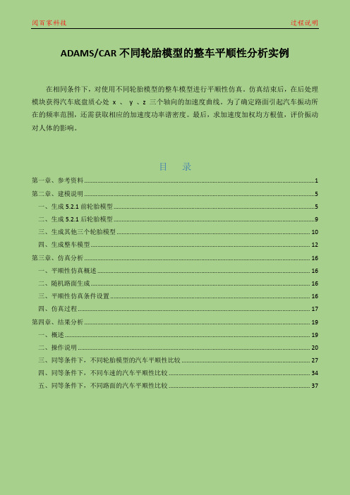
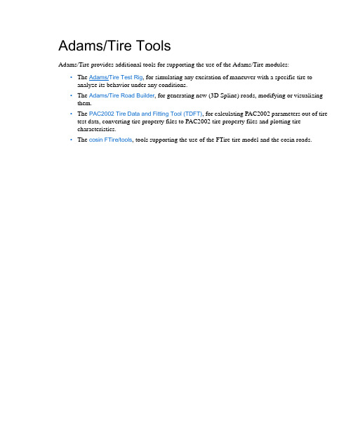
ADAMS/CAR不同轮胎模型的整车平顺性分析实例在相同条件下,对使用不同轮胎模型的整车模型进行平顺性仿真。
仿真结束后,在后处理模块获得汽车底盘质心处x 、y 、z 三个轴向的加速度曲线。
为了确定路面引起汽车振动所在的频率范围,还需获取相应的加速度功率谱密度。
最后,求加速度加权均方根值,评价振动对人体的影响。
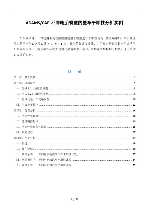
目录第一章、参考资料 (1)第二章、建模说明 (5)一、生成5.2.1前轮胎模型 (5)二、生成5.2.1后轮胎模型 (9)三、生成其他三个轮胎模型 (10)四、生成整车模型 (12)第三章、仿真分析 (16)一、平顺性仿真概述 (16)二、随机路面生成 (16)三、平顺性仿真条件设置 (16)四、仿真过程 (17)第四章、结果分析 (19)一、概述 (19)二、操作说明 (20)三、同等条件下,不同轮胎模型的汽车平顺性比较 (27)四、同等条件下,不同车速的汽车平顺性比较 (34)五、同等条件下,不同路面的汽车平顺性比较 (37)第一章、参考资料在ADAMS虚拟样机仿真软件中按照实际使用情况可将轮胎模型分为操作性分析轮胎模型、耐久性分析即3D接触分析轮胎模型以及摩托车用轮胎模型三大类。
由于本文中主要研究的是轮胎与路面间垂直力所引起的冲击振动情况,故应选用操纵性分析轮胎模型,其使用的是point follower的方式来计算轮胎由于路面不平激励所引起的垂直力。
在操纵性分析轮胎模型组中提供了MF-tyre、Pacejka ’89、Pacejka ’94、PAC2002、Fiala、5.2.1以及UA等轮胎模型,用户可以根据实际需要对模型数据进行修改。
通过修改软件自带的轮胎模型文件来生成轮胎模型能够保证车辆仿真要求的一致性,从而保证仿真结果的可靠性。
第二章、建模说明一、生成5.2.1前轮胎模型为建立轮胎模型,需先将acar共享文件中需要的轮胎数据复制到个人文件夹,本文进行汽车平顺性分析,适用于平顺性分析的轮胎模型有MF-tyre、Pacejka ’89、Pacejka ’94、PAC2002、Fiala、5.2.1以及UA等轮胎模型,本文选取4种类型:521_equation、mdi_fiala01、mdi_pac94、uat。
轮胎模型-PPT精品文档
• 二、 用于耐久性分析的轮胎模型
• 三维接触模型,考虑了轮胎胎侧截面的几何特性,并把轮 胎沿宽度方向离散,用等效贯穿体积的方法来计算垂直力, 可以用于三维路面。该模型是一个单独的License,但是如 果用户只购买Durability TIRE,只能用Fiala模型计算操稳。 • 除了上述两类模型以外,还有环模型,作为子午线轮胎的 近似,研究轮胎本身的振动特性,成为国际上仿真轮胎在 短波不平路面动特性的主流模型,是目前发展比较成熟和 得到商业化应用的轮胎模型,其中具有代表性的是F-tire和 SWIFT轮胎模型。
• SWIFT模型(Short Wave Intermediate Frequency TIRE Model) • SWIFT 模型是由荷兰 Delft 工业大学和 TNO 联合开发的,是 一个刚性环模型,在环模型的基础上只考虑轮胎的 0阶转动 和1阶错动这两阶模态,此时轮胎只作整体的刚体运动而并 不发生变形。在只关心轮胎的中低频特性时可满足要求。由 于不需要计算胎体的变形,刚性环模型的计算效率大大提高, 可用于硬件在环仿真进行主动悬架和ABS的开发。在处理面 外动力学问题时,SWIFT使用了魔术公式。
轮胎模型
一、轮胎模型简介 二 、ADAMS/TIRE 三、轮胎的特性文件
严金霞
2009年1月
• 轮胎是汽车重要的部件,它的结构参数和力学特性决定 着汽车的主要行驶性能。轮胎所受的垂直力、 纵向力、 侧向力和回正力矩对汽车的平顺性、 操纵稳定性和安全 性起重要作用。 • 轮胎模型对车辆动力学仿真技术的发展及仿真计算结果 有很大影响,轮胎模型的精度必须与车辆模型精度相匹 配。因此,选用轮胎模型是至关重要的。由于轮胎具有 结构的复杂性和力学性能的非线性,选择符合实际又便 于使用的轮胎模型是建立虚拟样车模型的关键。
ADAMS轮胎试验台(Tire Testrig)使用方法
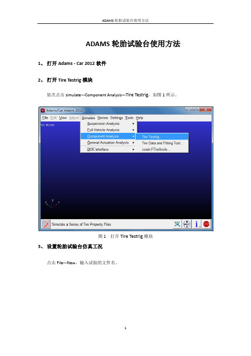
ADAMS轮胎试验台使用方法1、打开Adams - Car 2012软件2、打开Tire Testrig模块依次点击simulate---Component Analysis---Tire Testrig,如图1所示。
图1 打开Tire Testrig模块3、设置轮胎试验台仿真工况点击File---New,输入试验的文件名。
图2 新建试验台1、选择轮胎标签2、选择轮胎特性文件3、设置轮胎质量、转动惯量图3 轮胎设置图4 路面设置图5 轮胎运动设置 1、选择路面标签 2、选择路面类型,如平路面、凸块、路面文件3、设定路面运动方式1、选择轮胎运动标签2、轮胎纵向初速度3、轮胎旋转运动,可以设置纵向滑移率1、选择轮胎负载标签2、设置垂向力或运动3、设置纵向力或运动4、设置制动力矩图6 轮胎负载的设置1、选择平台输出标签2、设置平台侧向输入3、设置平台倾角图7 试验平台输出设置图8 弹簧、减震器设置4、 轮胎试验仿真在任意界面点击Run It ,如图9所示。
本试验工况为:轮胎特性文件为pac2002_195_65R15.tir ;路面为平路面;车轮质心纵向速度为20m/s ,车轮质心垂直加载为3000N ;轮胎侧偏角按正弦波变化,波峰为15度。
图9 开始仿真5、 仿真结果仿真结束后会自动进入ADAMS 后处理模块,点击File---Import---Requestrian File,如图1、选择弹簧阻尼标签3、设置弹簧刚度4、设置阻尼2、设置垂向预加载10所示。
在出现的对话框的File Name,右击选择Search,选择结果文件所在的文件夹,如图11所示。
选中结果文件,点击打开,如图12所示。
图10 导入结果文件图11 选择结果文件图12 选中结果文件图13 后处理曲线选择Requests 设置曲线纵坐标设置曲线横坐标图14 轮胎侧偏角与时间曲线图15 轮胎侧向力与时间曲线图16 轮胎侧向力与侧偏角曲线。
基于ADAMS和CATIA的轿车前轮轮胎包络面的生成
基于ADAMS和CATIA的轿车前轮轮胎包络面的生成在汽车设计中,前轮轮胎是车辆上最易磨损的部件之一。
因此,在设计轿车前轮轮胎时,必须考虑到其实际使用情况,以确保其长期的耐用性和可靠性。
在这个过程中,ADAMS和CATIA这两个软件可以提供有力的帮助。
本文将介绍如何使用这两个软件生成轿车前轮轮胎的包络面,以确保其与车辆和其他部件的良好配合和工作效率。
首先,在使用ADAMS和CATIA进行轿车前轮轮胎的包络面生成之前,必须进行准确的3D建模和数据输入。
这需要详细的汽车结构和轮胎细节图,以及汽车整体的底盘尺寸、重量和受力情况等数据。
只有这样,才能有效地进行后续的分析和计算。
接下来,使用CATIA创建轮胎的3D模型。
在此过程中,必须指定轮胎的大小、形状、花纹和硬度等参数。
这些参数将对后续的性能分析和设计起到重要的作用。
CATIA还可以进行轮胎的装配和调整,以实现与车辆其他部件的良好配合和紧密结合。
这里的目标是确保轮胎的包络面完全符合汽车设计的要求,并能够在高速行驶和复杂路况下保持稳定和耐用。
最后,在ADAMS中进行分析和模拟。
ADAMS是一款用于机械系统建模、仿真和分析的专业软件。
在进行轿车前轮轮胎包络面生成之前,必须先进行相应的数据输入和参数调整。
通过ADAMS的分析和模拟,可以更准确地预测轮胎的性能和行驶效率,进而对设计进行优化和改进。
总之,在使用ADAMS和CATIA进行轿车前轮轮胎包络面的生成过程中,必须进行详细的数据输入和准确的3D建模。
只有这样,才能确保实际使用中的可靠性和耐用性。
此外,还要进行相应的分析和模拟,以实现轮胎的最佳设计和性能优化。
为了生成轿车前轮轮胎的包络面,需要进行详细的数据分析和建模。
包括车辆整体的底盘尺寸和重量,轮胎的大小、形状、花纹和硬度等参数。
下面我们将对这些数据进行分析。
底盘尺寸和重量:车辆底盘尺寸包括轴距、前悬长度、后悬长度、前轮距、后轮距以及车身长度、宽度和高度等。
adams_tire_tools
Adams/Tire provides additional tools for supporting the use of the Adams/Tire modules:
• The Adams/Tire Test Rig, for simulating any excitation of maneuver with a specific tire to
Adams/Tire Tools 5
Using the Road Builder
Opening an Existing 3D Spline Road Property File
To edit an existing 3D Spline Road property file, do one of the following: • From the File menu, select Open, and then browse for the desired file.
test data, converting tire property files to PAC2002 tire property files and plotting tire characteristics.
• The cosin FTire/tools, tools supporting the use of the FTire tire model and the cosin roads.
4 Adams/Tire
Using the Road Builder
Creating a 3D Spline Road Property File
To create a new 3D Spline Road property file: • From the File menu, select New. When you create a new 3D Spline Road property file, the default values of the road vertical are set to (0.0, 0.0, 1.0). Note that the road vertical is normalized at the Adams/Solver level.
轮胎模型 PPT课件

• FTire是高分辨率物理轮胎模型,需要每秒数百万次评价路 面,为了实现空间和时间分辨率,路面模型选择很重要。 RGR路面(规则的栅格路面)是一个高分辨率的路面模型, 它采用等距网格避免寻找三角单元的节点,可选带有弧形中 心线,是特别适合以满足需求的效率,准确性和灵活性的路 面模型。因此,除了简单的几何参数的障碍路面模型,RGR 路面是FTire的首选路面描述方法。
• 5)Fiala模型 是弹性基础上的梁模型,不考虑外倾和松弛长 度。当不把内倾角作为主要因数且把纵向滑移和横向滑移分 开对待的情况下,对于简单的操纵性分析可得到合理的结果。
• 适用范围:有效频率到0.5Hz,可以用于二维和三维路面, 当与2D路面作用时是点接触;当与3D路面作用时,等效贯 穿体积的方法来计算垂直力。
二维路面、三维路面,还支持3D三角网格路面;RGR路面 文件(规则的栅格路面);所有COSIN/ev 路面模型,包括 大量的被参数化的障碍定义的路面文件、滚筒的旋转鼓路 面和空间的试验场地 。 • 这些路面模型可在所有环境中的支持FTire ,且不需要单独 的许可证。
• 以下的路面模型需要各自软件的安装环境和许可证
5.80 MB 5.91 MB
0.21 s
0.28 s
•相对于不规则三角网格路面,RGR道路提供大量和可扩展 的减少文件大小,减小内存的需求,减少文件加载时间和 CPU评价的时间。
• FTire提供了一个辅助程序FTire/roadtools工具箱来产生, 分 析 和 处 理 所 有 的 道 路 文 件 , 包 括 RGR 路 面 模 型 。
ADAMS轮胎模型简介

详细介绍轮胎模型,主要是自己做课题时,用到的整理汇总出来的,轮胎这部分的资料比较少的,记录下来帮助大家一起学习一起进步;主要分以下两部分介绍一、轮胎模型简介轮胎是汽车重要的部件,它的结构参数和力学特性决定着汽车的主要行驶性能。
轮胎所受的垂直力、纵向力、侧向力和回正力矩对汽车的平顺性、操纵稳定性和安全性起重要作用。
轮胎模型对车辆动力学仿真技术的发展及仿真计算结果有很大影响,轮胎模型的精度必须与车辆模型精度相匹配。
因此,选用轮胎模型是至关重要的。
由于轮胎具有结构的复杂性和力学性能的非线性,选择符合实际又便于使用的轮胎模型是建立虚拟样车模型的关键。
一、轮胎模型简介轮胎建模的方法分为三种:1)经验—半经验模型针对具体轮胎的某一具体特性。
目前广泛应用的有Magic Formula公式和吉林大学郭孔辉院士利用指数函数建立的描述轮胎六分力特性的统一轮胎半经验模型UniTire,其主要用于车辆的操纵动力学的研究。
2)物理模型根据轮胎的力学特性,用物理结构去代替轮胎结构,用物理结构变形看作是轮胎的变形。
比较复杂的物理模型有梁、弦模型。
特点是具有解析表达式,能探讨轮胎特性的形成机理。
缺点是精确度较经验—半经验模型差,且梁、弦模型的计算较繁复。
3)有限元模型基于对轮胎结构的详细描述 ,包括几何和材料特性,精确的建模能较准确的计算出轮胎的稳态和动态响应。
但是其与地面的接触模型很复杂,占用计算机资源太大,在现阶段应用于不平路面的车辆动力学仿真还不现实,处于研究阶段。
主要用于轮胎的设计与制造二、ADAMS/TIRE轮胎不是刚体也不是柔体,而是一组数学函数。
由于轮胎结构材料和力学性能的复杂性和非线性以及适用工况的多样性,目前还没有一个轮胎模型可适用于所有工况的仿真,每个轮胎模型都有优缺点和适用的范围。
必须根据需要选择合适的轮胎模型。
ADAMS/TIRE分为两大类:一).用于操稳分析的轮胎模型魔术公式是用三角函数的组合公式拟合轮胎试验数据,用一套形式相同的公式完整地表达轮胎的纵向力、侧向力、回正力矩、翻转力矩、阻力矩以及纵向力、侧向力的联合作用工况,主要包括以下的前四种模型。
ADAMS-CAR不同轮胎模型的整车平顺性分析实例
ADAMS/CAR不同轮胎模型的整车平顺性分析实例在相同条件下,对使用不同轮胎模型的整车模型进行平顺性仿真。
仿真结束后,在后处理模块获得汽车底盘质心处x 、y 、z 三个轴向的加速度曲线。
为了确定路面引起汽车振动所在的频率范围,还需获取相应的加速度功率谱密度。
最后,求加速度加权均方根值,评价振动对人体的影响。
目录第一章、参考资料 (1)第二章、建模说明 (5)一、生成5.2.1前轮胎模型 (5)二、生成5.2.1后轮胎模型 (9)三、生成其他三个轮胎模型 (10)四、生成整车模型 (12)第三章、仿真分析 (16)一、平顺性仿真概述 (16)二、随机路面生成 (16)三、平顺性仿真条件设置 (16)四、仿真过程 (17)第四章、结果分析 (19)一、概述 (19)二、操作说明 (20)三、同等条件下,不同轮胎模型的汽车平顺性比较 (27)四、同等条件下,不同车速的汽车平顺性比较 (34)五、同等条件下,不同路面的汽车平顺性比较 (37)第一章、参考资料在ADAMS虚拟样机仿真软件中按照实际使用情况可将轮胎模型分为操作性分析轮胎模型、耐久性分析即3D接触分析轮胎模型以及摩托车用轮胎模型三大类。
由于本文中主要研究的是轮胎与路面间垂直力所引起的冲击振动情况,故应选用操纵性分析轮胎模型,其使用的是point follower的方式来计算轮胎由于路面不平激励所引起的垂直力。
在操纵性分析轮胎模型组中提供了MF-tyre、Pacejka ’89、Pacejka ’94、PAC2002、Fiala、5.2.1以及UA等轮胎模型,用户可以根据实际需要对模型数据进行修改。
通过修改软件自带的轮胎模型文件来生成轮胎模型能够保证车辆仿真要求的一致性,从而保证仿真结果的可靠性。
第二章、建模说明一、生成5.2.1前轮胎模型为建立轮胎模型,需先将acar共享文件中需要的轮胎数据复制到个人文件夹,本文进行汽车平顺性分析,适用于平顺性分析的轮胎模型有MF-tyre、Pacejka ’89、Pacejka ’94、PAC2002、Fiala、5.2.1以及UA等轮胎模型,本文选取4种类型:521_equation、mdi_fiala01、mdi_pac94、uat。
基于ADAMS的车轮定位参数优化设计

在我国, 许多车型出现了轮胎早期磨损严重、前 轮摆振、转向沉重等现象。产生这种现象的主要原因 之一是因为在汽车设计过程中,车轮定位参数的选取 还处于纯经验阶段,各参数之间的配合关系也没有足 够的理论指导,从而导致轮胎受力不均衡,异常磨损 严重。因此,本文对车轮定位参数进行全面、系统的分 析,研究在车轮跳动过程中,定位参数与轮胎磨损之
4 基于轮胎最小侧滑的车轮定位参数优化
主销内倾角越大, 越有利于减小轮胎的磨损,但 是主销内倾角过大,会使转向发飘,反而增大轮胎的 磨损,所以主销内倾角应约束在 3° ̄12°的范围内。主 销后倾角越大, 越有助于保持车辆行驶的方向稳定 性,但过大的主销后倾角可能导致不平顺的行驶状况, 若在低速,甚至会导致转向前轮产生摆振,因此主销后 倾角宜在 3° ̄6°的范围内。在车轮跳动过程中,车轮外 倾角对轮胎的侧滑影响小,但是,外倾角过大,会使轮 胎出现偏磨损现象, 故车轮外倾角约束在 0.5° ̄2°的 范围内。对于前束角,用公式 1 限制其取值范围。
本文应用 ADAMS 软 件 建 立 了 汽 车 前 悬 架 —转 向系统仿真模型。目前国外许多汽车企业都已经大 规模应用仿真系统进行汽车的运动学和动力学分析, 使设计中的主要问题利用数字化虚拟样机技术在设 计初期就得以解决。
前 悬 架 — 转 向 系 统 仿 真 模 型 由 转 向 节 、车 轮 、主 销 、转 向 节 臂 、转 向 横 拉 杆 及 测 试 台 等 刚 体 组 成 , 如 图 1 所示。主销用万向节铰与上、下横臂相连,转向节与 主销用旋转铰约束,转向横拉杆通过球铰与转向节臂 相连。车轮总成和转向节总成通过转动铰链相连。
不宜过小。而随着后倾角的增大,外倾角的变化减小,
所 以 后 倾 角 应 取 较 大 的 值(对 外 倾 角 的 影 响 不 如 内 倾
ADAMS轮胎模型简介
详细介绍轮胎模型,主要是自己做课题时,用到的整理汇总出来的,轮胎这部分的资料比较少的,记录下来帮助大家一起学习一起进步;主要分以下两部分介绍一、轮胎模型简介轮胎是汽车重要的部件,它的结构参数和力学特性决定着汽车的主要行驶性能。
轮胎所受的垂直力、纵向力、侧向力和回正力矩对汽车的平顺性、操纵稳定性和安全性起重要作用。
轮胎模型对车辆动力学仿真技术的发展及仿真计算结果有很大影响,轮胎模型的精度必须与车辆模型精度相匹配。
因此,选用轮胎模型是至关重要的。
由于轮胎具有结构的复杂性和力学性能的非线性,选择符合实际又便于使用的轮胎模型是建立虚拟样车模型的关键。
一、轮胎模型简介轮胎建模的方法分为三种:1)经验—半经验模型针对具体轮胎的某一具体特性。
目前广泛应用的有 Magic Formula公式和吉林大学郭孔辉院士利用指数函数建立的描述轮胎六分力特性的统一轮胎半经验模型UniTire ,其主要用于车辆的操纵动力学的研究。
2)物理模型根据轮胎的力学特性,用物理结构去代替轮胎结构,用物理结构变形看作是轮胎的变形。
比较复杂的物理模型有梁、弦模型。
特点是具有解析表达式,能探讨轮胎特性的形成机理。
缺点是精确度较经验—半经验模型差,且梁、弦模型的计算较繁复。
3)有限元模型基于对轮胎结构的详细描述 , 包括几何和材料特性,精确的建模能较准确的计算出轮胎的稳态和动态响应。
但是其与地面的接触模型很复杂,占用计算机资源太大,在现阶段应用于不平路面的车辆动力学仿真还不现实,处于研究阶段。
主要用于轮胎的设计与制造二、 ADAMS/TIRE轮胎不是刚体也不是柔体,而是一组数学函数。
由于轮胎结构材料和力学性能的复杂性和非线性以及适用工况的多样性,目前还没有一个轮胎模型可适用于所有工况的仿真,每个轮胎模型都有优缺点和适用的范围。
必须根据需要选择合适的轮胎模型。
ADAMS/TIRE分为两大类:一) .用于操稳分析的轮胎模型魔术公式是用三角函数的组合公式拟合轮胎试验数据,用一套形式相同的公式完整地表达轮胎的纵向力、侧向力、回正力矩、翻转力矩、阻力矩以及纵向力、侧向力的联合作用工况,主要包括以下的前四种模型。
adams培训教程
-Chapter
7
•
由于多体系统的复杂性,在建立系统的动力学
方程时,采用系统独立的拉格朗日坐标将非常困难
,而采用不独立的笛卡尔广义坐标比较方便;对具
具有多余坐标的完整或非完整约束系统,用带乘子
的拉氏方程处理是十分规格化的方法。导出的以笛
卡尔广义坐标为变量的动力学方程是与广义坐标数
目相同的带乘子的微分方程,还需要补充广义坐标
机器是由若干机构组成的系统。根据机械系统组成的运动 形式,在虚拟样机系统中,将零件和构件统称为构件,将机构 和机器统称为机械系统或样机,而机械系统或样机是由若干个 构件通过不同的运动副相互连接组成的。
-Chapter
12
机械系统虚拟样机研究的问题
• 对于复杂机械系统人们关心的问题大致有三类:
• 运动学分析: 在不考虑系统运动起因的情况下研究各 部件的位置与姿态及其他们变化速度与加速度的关系 。
-Chapter
3ห้องสมุดไป่ตู้
Chapter 1: 绪论
• 虚拟样机技术的基本概念 • 虚拟样机技术的理论基础 • 虚拟样机技术的发展过程 • ADAMS虚拟样机软件系统概述
-Chapter
4
虚拟样机技术的基本概念
• 虚拟样机技术是指在产品设计开发过程中 ,将分散的零部件设计和分析技术(指在某 单一系统中零部件的CAD和FEA技术)揉合在 一起,在计算机上建造出产品的整体模型 ,并针对该产品在投人使用后的各种工况 进行仿真分析,预测产品的整体性能,进 而改进产品设计、提高产品性能的一种新 技术。
CAT/ADAMS(與 CATIA 整合的介
A/Car、A/Driver、A/Tire 及 A/Pre
面)
等)
Adams基础培训

ADAMS/View 基本环境
ADAMS/Solver 求解器
ADAMS/PostProcessor 后处理
11
ADAMS简单教程
ADAMS/View
可以像建立物理样机一样建立任何机械系统的虚 拟样机。首先建立运动部件(或者从CAD软件中 导入)、用约束将它们连接、通过装配成为系统、 利用外力或运动将他们驱动。
RPC Pro Fatigue Tools
Integrated ADAMS loads transfer to FE-Fatigue tools
FE-Fatigue
MSC.Fatigue
FE Pre/Post processors an e.g. Ansys, Abaqus, Hypermesh,
Patran.
• 自行定义对话框
Taguchi Method JMP, SAS, SPSS
Excel…...
4
ADAMS简单教程
MSC.ADAMS的发展史简介
ADAMS(Automatic Dynamic Analysis of Mechanical
Systems):
机械系统自动化动力学仿真软件。
虚拟样机(Virtual Prototyping)流程
BUILD
• 构建模型 (部件、载荷、接触、碰撞、约束、驱动等) • 输入 CAD 模型
TEST VALIDATE
REFINE ITERATE
• •
构执建行驱 初动 步器 机构,I-传D模感E拟A器S((se仿ns真or、s)与动构画建、测曲量线)( measureMMs) AATTRLAIXB
ADAMS/Durability
耐久性分析模块
ADAMS2005李军整车模型轮胎问题
ADAMS2005李军整车模型轮胎问题(附模型仿真视频)我近来也在做李军的整车模型,用的是ADAMS2005R2,全部做好了,包括路面和轮胎都加好了。
但仿真时,除了轮胎外车子老往下掉,轮胎停在路面和车身脱离。
我估计是轮胎没加好。
但轮胎和车子间除了一个MARKER点的LOCATION外,好像没什么关联。
尝试在TIRE和轴间加旋转副,车子虽然不往下掉,但不动了。
大家能给我些建议吗?十分感谢!!我的QQ53434666,Email:fgg365※下面附件里是我的模型仿真视频。
[本帖最后由okchina 于2006-8-6 13:06 编辑]附件2006-8-3 17:19下载次数: 163car.rar(220.58 KB)模型仿真视频引用报告回复新手会员UID 164028 精华 0 积分 0 帖子 21 贡献积分 2 阅读权限 10 注册 2006-4-28 状态 离线大 中 小使用道具发表于 2006-8-4 10:28 资料 个人空间 短消息 加为好友这个模型从置顶的帖子看应该又很多人做过 大家帮忙给出出建议吧 谢谢引用 报告 回复新手会员UID 164028 精华 0 积分 0 帖子 21 贡献积分 2 阅读权限 10 注册 2006-4-28 状态 离线大 中 小使用道具发表于 2006-8-6 13:03 资料 个人空间 短消息 加为好友自己顶起来 高手看到给给意见引用 报告 回复celery 新手会员UID 161855 精华 0 积分 0 帖子 51 贡献积分 5 阅读权限 10 注册 2006-4-11 状态 离线#4 大 中 小使用道具发表于 2006-8-14 10:59 资料 个人空间 短消息 加为好友以前有战友总结过的,你在网内搜索下应该可以找到答案的引用 报告 回复jac_lance (lance) 新手会员UID 55345 精华 0 积分 1 帖子 52 贡献积分 11 阅读权限 10 注册 2004-7-14 来自 0551 状态 离线#5 大 中 小使用道具发表于 2006-8-16 13:14 资料 个人空间 短消息 加为好友在轮胎和转向节之间加旋转副是对的,车子不动是你没有加运动建议你把轮胎和路面之间的距离设小一点,先做一下静平衡,再进行仿真,应该没问题,如不行可和我联系, jac_lance@引用 报告 回复okchina 新手会员UID 164028 精华 0 积分 0 帖子 21 贡献积分 2 阅读权限 10 注册 2006-4-28 状态 离线#6 大 中 小使用道具发表于 2006-8-16 19:30 资料 个人空间 短消息 加为好友谢谢楼上的建议我后来发现掉下去的原因是路面加反了 仿真开始用的是UA 轮胎和普通的2D 路面 动作不明显将轮胎改为FLALA 的好多了 加上3D 路面现在也都可以 但我的模型静平衡总通不过'所谓的静平衡到现在仍然是迷迷糊糊 不是很清楚不知道楼上的有相关资料不引用 报告 回复jac_lance (lance) 新手会员UID 55345精华 0积分 1帖子 52贡献积分 11阅读权限 10 注册 2004-7-14 来自 0551 状态 离线#7 大 中 小使用道具发表于 2006-8-18 12:09 资料 个人空间 短消息 加为好友static equilifrium对于你这模型而言,静平衡是在进行动力学分析前所做的一种状态寻找,此举目的是计算有多自由度模型中内力外力共同作用的平衡状态,其中速度和加速度设为0.我理解: 静平衡是考虑到模型在进行动力学仿真初时,受力有突变,容易造成计算不稳定,静平衡跳过此段时间,即忽略了瞬态.详细解释帮助里有: seach " static equilifrium"引用 报告 回复okchina 新手会员UID 164028 精华 0 积分 0 帖子 21 贡献积分 2 阅读权限 10 注册 2006-4-28 状态 离线#8 大 中 小使用道具发表于 2006-8-21 14:58 资料 个人空间 短消息 加为好友谢谢搂上的解答看来静平衡是个很难调整的东西 我的一直也调整不好看来做整车还是在car 里做好些 另外在VIEW 里,整车比如蛇行线等的试验好像也很困难引用 报告 回复zzyhnhtth 新手会员UID 140060 精华 0 积分 0 帖子 26 贡献积分 11 阅读权限 10 注册 2005-11-10 状态 离线#9 大 中 小使用道具发表于 2006-12-18 14:13 资料 个人空间 短消息 加为好友我下下来试试我以前也做过,一直做不好引用 报告 回复wusley 新手会员UID 203331 精华 0 积分 0 帖子 4 贡献积分 4 阅读权限 10 注册 2006-10-30 来自 江西 状态 离线#10 大 中 小使用道具发表于 2006-12-23 13:46 资料 个人空间 短消息 加为好友怎么编写轮胎和地面谱的特性文件啊 急~~~~~ 有哪位知道的还望指教引用 报告 回复www97810新手会员UID 169935精华 0积分 0帖子 6贡献积分 3阅读权限 10注册 2006-6-7状态 离线 #11 大 中 小 使用道具 发表于 2006-12-24 10:01 资料 个人空间 短消息 加为好友我也说两句,最近有没有碰到仿真时总出现警告信息:longitudinal slip ratio>1的情况,而且只是出现在后轮上,怎么解决???引用 报告 回复shuzhan新手会员UID 241682精华 0积分 0帖子 10贡献积分 3阅读权限 10注册 2007-3-9状态 离线#12 大 中 小 使用道具 发表于 2007-3-10 10:46 资料 个人空间 短消息 加为好友楼主这问题提的好啊也不知道怎么回事,李军整车联系,在做的过程,总是有问题.好象还没听说有很顺利的做出来的。
ADAMS轮胎模型简介

详细介绍轮胎模型,主要是自己做课题时,用到的整理汇总出来的,轮胎这部分的资料比较少的,记录下来帮助大家一起学习一起进步;主要分以下两部分介绍一、轮胎模型简介轮胎是汽车重要的部件,它的结构参数和力学特性决定着汽车的主要行驶性能。
轮胎所受的垂直力、纵向力、侧向力和回正力矩对汽车的平顺性、操纵稳定性和安全性起重要作用。
轮胎模型对车辆动力学仿真技术的发展及仿真计算结果有很大影响,轮胎模型的精度必须与车辆模型精度相匹配。
因此,选用轮胎模型是至关重要的。
由于轮胎具有结构的复杂性和力学性能的非线性,选择符合实际又便于使用的轮胎模型是建立虚拟样车模型的关键。
一、轮胎模型简介轮胎建模的方法分为三种:1)经验—半经验模型针对具体轮胎的某一具体特性。
目前广泛应用的有Magic Formula公式和吉林大学郭孔辉院士利用指数函数建立的描述轮胎六分力特性的统一轮胎半经验模型UniTire,其主要用于车辆的操纵动力学的研究。
2)物理模型根据轮胎的力学特性,用物理结构去代替轮胎结构,用物理结构变形看作是轮胎的变形。
比较复杂的物理模型有梁、弦模型。
特点是具有解析表达式,能探讨轮胎特性的形成机理。
缺点是精确度较经验—半经验模型差,且梁、弦模型的计算较繁复。
3)有限元模型基于对轮胎结构的详细描述,包括几何和材料特性,精确的建模能较准确的计算出轮胎的稳态和动态响应。
但是其与地面的接触模型很复杂,占用计算机资源太大,在现阶段应用于不平路面的车辆动力学仿真还不现实,处于研究阶段。
主要用于轮胎的设计与制造二、ADAMS/TIRE轮胎不是刚体也不是柔体,而是一组数学函数。
由于轮胎结构材料和力学性能的复杂性和非线性以及适用工况的多样性,目前还没有一个轮胎模型可适用于所有工况的仿真,每个轮胎模型都有优缺点和适用的范围。
必须根据需要选择合适的轮胎模型。
ADAMS/TIRE分为两大类:一).用于操稳分析的轮胎模型魔术公式是用三角函数的组合公式拟合轮胎试验数据,用一套形式相同的公式完整地表达轮胎的纵向力、侧向力、回正力矩、翻转力矩、阻力矩以及纵向力、侧向力的联合作用工况,主要包括以下的前四种模型。
ADAMS魔术公式的轮胎模型
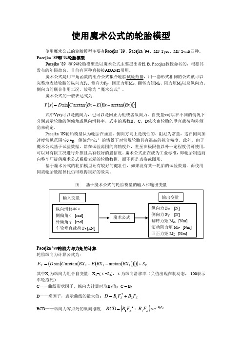
使用魔术公式的轮胎模型使用魔术公式的轮胎模型主要有Pacejka ’89、Pacejka ’94、MF-Tyre 、MF-Swift 四种。
Pacejka ’89和’94轮胎模型Pacejka ’89 和’94轮胎模型是以魔术公式主要提出者H. B. Pacejka 教授命名的,根据其发布的年限命名。
目前有两种直接被ADAMS 引用。
魔术公式是用三角函数的组合公式拟合轮胎试验数据,用一套形式相同的公式就可以完整地表达轮胎的纵向力F x 、侧向力F y 、回正力矩M z 、翻转力矩M x 、阻力矩M y 以及纵向力、侧向力的联合作用工况,故称为“魔术公式”。
魔术公式的一般表达式为:()()(){}[]Bx Bx E Bx C D x Y arctan arctan sin --=式中Y(x)可以是侧向力,也可以是回正力矩或者纵向力,自变量x 可以在不同的情况下分别表示轮胎的侧偏角或纵向滑移率,式中的系数B 、C 、D 依次由轮胎的垂直载荷和外倾角来确定。
Pacejka ’89轮胎模型认为轮胎在垂直、侧向方向上是线性的、阻尼为常量,这在侧向加速度常见范围≤0.4g ,侧偏角≤5°的情景下对常规轮胎具有很高的拟合精度。
此外,由于魔术公式基于试验数据,除在试验范围的高精度外,甚至在极限值以外一定程度仍可使用,可以对有限工况进行外推且具有较好的置信度。
魔术公式正在成为工业标准,即轮胎制造商向整车厂提供魔术公式系数表示的轮胎数据,而不再是表格或图形。
基于魔术公式的轮胎模型还有较好的健壮性,如果没有某一轮胎的试验数据,而使用同类轮胎数据替代仍可取得很好的效果。
图 基于魔术公式的轮胎模型的输入和输出变量Pacejka ’89轮胎力与力矩的计算 轮胎纵向力计算公式为:()()()()()V X S BX BX E BX C D F +--=111arctan arctan sin其中X 1为纵向力组合自变量:X 1=(κ+S h ),κ为纵向滑移率(负值出现在制动态,-100表示车轮抱死)C ——曲线形状因子,纵向力计算时取B 0值:C = B 0D ——巅因子,表示曲线的最大值:Z Z F B F B D 221+= BCD ——纵向力零点处的纵向刚度:()ZF B Z Z eF B F B BCD 5423-⨯+=B – 刚度因子:B=BCD/(C ×D)S h ——曲线的水平方向漂移:109B F B S Z h += S v ——曲线的垂直方向漂移:S v =0E ——曲线曲率因子,表示曲线最大值附近的形状:8726BF B F B E Z Z ++=图 轮胎属性文件中的纵向力计算系数数据块图 Pacejka ’89轮胎纵向力示例轮胎侧向力计算公式为:()()()()()V Y S BX BX E BX C D F +--=111arctan arctan sin此时的X 1为侧向力计算组合自变量:X 1=(α+S h ),α为侧偏角 C ——曲线形状因子,侧向力计算时取A 0值:C = A 0 D ——巅因子,表示曲线的最大值:Z Z F A F A D 221+=BCD ——侧向力零点处的侧向刚度:()γ5431arctan 2sin A A F A BCD Z -⨯⎪⎪⎭⎫⎝⎛= B – 刚度因子:B=BCD/(C ×D)S h ——曲线的水平方向漂移:γ8109A A F A S Z h ++=曲线形状因子巅因子计算系数 BCD 计算系数 曲线水平漂移计算系数曲线曲率因子计算系数S v ——曲线的垂直方向漂移:131211A F A F A S Z Z V ++=γE ——曲线曲率因子,表示曲线最大值附近的形状:76AF A E Z +=图 轮胎属性文件中的侧向力计算系数数据块图 Pacejka ’89轮胎纵向力示例轮胎回正力矩计算公式为:()()()()()V Z S BX BX E BX C D M +--=111arctan arctan sin此时的X 1为回正力矩计算组合自变量:X 1=(α+S h ),α为侧偏角 C ——曲线形状因子,回正力矩计算时取C 0值:C = C 0 D ——巅因子,表示曲线的最大值:Z Z F C F C D 221+=BCD ——回正力矩零点处的扭转刚度:()()ZF C Z Z e C F C F C BCD 564231-⨯-⨯+=γB – 刚度因子:B=BCD/(C ×D)S h ——曲线的水平方向漂移:131211C F C C S Z h ++=γ曲线形状因子巅因子计算系数 BCD 计算系数 曲线水平漂移计算系数 曲线曲率因子计算系数 曲线垂直漂移计算系数S v ——曲线的垂直方向漂移:()171615214C F C F C F C S Z Z Z V +++=γE ——曲线曲率因子,表示曲线最大值附近的形状:()()γ1098271C C F C F C E Z Z -⨯++=图 轮胎属性文件中的回正力矩计算系数数据块图 Pacejka ’89轮胎回正力矩示例侧偏刚度(Lateral Stiffness )侧偏刚度在Pacejka ’89和’94轮胎模型中假定是一个常量,在轮胎属性文件的参数PARAMETER 数据段中通过LATERAL_STIFFNESS 语句设定。
ADAMS培训教程

边缘倒角、边缘圆角、开孔、添加凸台、 挖空或在外围添加材料
要求圆角半径变化时,需选择 End Radius 项,输入末端半径值,此时圆角半径为起 始半径 开孔 Hole 半径(Radius),深度(Depth) 半径和深度的设置,不能使几何体分成两 块 凸圆 挖空 Hollow Boss 半径(Radius),高度(Height) 壳体厚度 t(Thickness)
限自由度 工具图标 名 称 图 例 移动 转动
转动副
3
2
移动副
2
3
圆柱副
2
2
球形副
3
0
运动副约束(简单)
限自由度 工具图标 名 称 图 例 移动 转动
平面副
1
2
恒速副
3
1
虎克铰
3
1
固定副
3
3
运动副约束(复杂) 螺旋副:限制3个移动,2个转动。 常配合一个移动副使用。
运动副约束(复杂) 关联副:常用于关联转动副和移动副。
按照屏幕下方状态栏的提示,用鼠标确定 起始绘图点
定义了几何形体的位置,自动在起始点设置一
简单形体几何建模
几何建 模工具 几何建模工 具集
表格编 辑器
组合形体
细节 浮动对 话框 设置栏
ADAMS/View基本形体图库
名称和 快捷键 长方体 Box 图 形 尺寸参数/默认值 尺寸参数 默认值 长(Length) 高(Height) 深(Depth)/2min(长, 高) 长(Length) 半径(Radius)/0.25长 半径(Radii)/ x,y,z 三个方向的 半径相等 若x,y,z 三个方向半径不相等,生成 椭球。 长(Length) 底半径(Bottom Radius) /0.125长 顶半径(Top Radius) /0.5底半径 圆环半径(Inner Radius) 圆管半径(Outer Radius) /0.25圆环半径 说 明 绘图起始和结束点为长方体的 两个对角端点。有1个热点, 定义长、高和深 绘图起始点为中心点。 有2个亮点可分别用于修改长 度和半径 绘图起始点为中心点。 有3个亮点,可分别用于修改 x,y,z 方向的半径 圆柱体 Cylinder
- 1、下载文档前请自行甄别文档内容的完整性,平台不提供额外的编辑、内容补充、找答案等附加服务。
- 2、"仅部分预览"的文档,不可在线预览部分如存在完整性等问题,可反馈申请退款(可完整预览的文档不适用该条件!)。
- 3、如文档侵犯您的权益,请联系客服反馈,我们会尽快为您处理(人工客服工作时间:9:00-18:30)。
• ADAMS/Tire操纵性轮胎模块采用 point-follower 的方法计算轮胎的 正压力并且限于二维的路面模型。 注释:* Pacejka 轮胎模型中所使用计算公式来源于 H.B. Pacejka 博士公开发表的文献,在汽车行业通常指的是 Pacejka 模型。Dr. Pacejka 本人既没有参与这些轮胎模型的开发,也未 以任何方式资助其开发。
• 所有的轮胎模块都支持 ADAMS/Linear 的功能。
MSC Confidential
ADAMS/Tire 模块
• ADAMS/Tire 模块的特色
• 下表列出了 ADAMS/Tire 中各轮胎模块的特色。
MSC Confidential
ADAMS/Tire 模块
• 你应该使用什么类型的轮胎?
• • • • • ADAMS/Tire Handling Module Adams/Tire 3D Shell Road – 先前称为3D Contact Adams/Tire 3D Spline Road –先前称为3D Smooth Road model Specific Tire Models Features in ADAMS/Tire Modules
• ADAMS/Tire 允许你在一个车辆模型中最多可以有 40 个 轮胎。
MSC Confidential
ADAMS/Tire 模块
• ADAMS/Tire 有一系列的轮胎模块,你可以结合 ADAMS/View、 ADAMS/Solver、ADAMS/Car和 ADAMS/Chassis使用。这些模 块使你能够模拟常见的各种车辆如:轿车、卡车或飞机上的橡胶 轮胎。特别是,这些轮胎模块可以模拟轮胎上产生的力以使车辆 加速、制动或转向等。在 ADAMS/Tire 中可以用的轮胎模块有:
MSC Confidential
路面类型
• 二维路面的接触采用 point-follower 的方法 (类似于一张平面 的圆盘)。下面为使用这种方法所用的不同的路面类型 (主要 是对应 FTIRE):
• DRUM - Tire test drum (requires a zero-speed-capable tire model). • FLAT - Flat road. • PLANK - Single plank perpendicular, or in oblique direction relative to x-axis, with or without bevel edges. • POLY_LINE - Piece-wise linear description of the road profile. The profiles for the left and right track are independent. • POT_HOLE - Single pothole of rectangular shape. • RAMP - Single ramp, either rising or falling. • ROOF - Single roof-shaped, triangular obstacle.
MSC Confidential
路面类型
• SINE - Sine waves with constant wave length. • SINE_SWEEP - Sine waves with decreasing wave lengths. • STOCHASTIC_UNEVEN - Synthetically generated irregular road profiles that match measured stochastic properties of typical roads. The profiles for left and right track are independent, or may have a certain correlation.
MSC Confidential
使用 3D 等效体积路面模型
• 定义 3D 等效体积路面模型
• 你需要使用一个路面特性文件来定义三维路面。路面特性文件包含五个 数据块:Header、Units、Model、Nodes和Elements。这些数据块可 以按照任意的顺序出现在文件中,并且关键字可以放在其所属的数据块 的任何顺序。
MSC Confidential
使用 3D 等效体积路面模型 • 关于3D 等效体积路面模型
• 3D 等效体积路面模型为一般的三维表面, 并用一系列的三角形片表示。右侧的图表示 一个由编号为 1 到 6 的六个节点构成的路 表面。六个节点共构成四个三角形的面单元, 分别表示为 A、B、 C 和 D。每个三角形单 元的向外的单位法向矢量如图所示。与有限 元中网格的定义习惯非常相似, ADAMS/Tire 在定义路面时需要你首先指定 每个节点在路面的参考坐标系下的坐标,然 后再按照顺序指定由三个节点构成的三角形 单元,对应每个单元,你可以指定不同的摩 擦系数。
• ADAMS/Chassis中各种类型路面的样板文件在:
• install_dir /achassis examples/rdf/
MSC Confidential
2D 路面的例子 (RAMP)
MSC Confidential
使用3D轮廓路面模型
• ADAMS/Tire 3D Shell Road为三维的轮胎-路面接触模型,用来 计算路面和轮胎之间交叉的体积。路面是用一系列离散的三角 形片来表示,而轮胎则用一系列的圆柱表示。采用此路面模型, 你可以模拟车辆在运动过程中碰到路边台阶、凹坑或在粗糙路 面或不规则路面上运动的情形。
• 每个轮胎模块在一个特定的应用领域是正确的。超出这一领域可能会出 现不真实的分析结果。下图所示为每种类型的轮胎的正确适用领域,而 下页的表表明不同的轮胎模型的最佳应用情况。 • 通常来讲,ADAMS/Tire 的操纵性轮胎模块只适用于相当光滑的路面: 路面障碍的波长不应当小于轮胎的周长。如果障碍的波长小于轮胎的周 长,你应该使用 SWIFT-Tyre 或 FTire 轮胎模型以考虑轮胎周边变形的 非线性的影响。 • 操纵性轮胎模块适用于描述轮胎的一阶响应,但是不考虑轮胎自身的特 征频率的影响。因此,操纵性轮胎模块适用于在 大约 8 Hz 频率以下的 响应分析(PAC 2002 轮胎15 Hz ) ,超过这一频率,轮胎模型就应该考 虑轮胎周边橡胶带的影响,FTire 轮胎模型就考虑了其影响。
MSC Confidential
ADAMS/Tire 模块
• ADAMS/Tire 操纵性轮胎模块
• ADAMS/Tire 操纵性轮胎模块包含下列可用于车辆动力学研究中的 轮胎模块:
• • • • • Pacejka 2002 tire model* Pacejka '89 and Pacejka '94 models* Fiala tire model UA tire model 5.2.1 tire model
MSC Confidential
ADAMS/Tire 模块
• ADAMS/Tire 3D 光滑路面模块
• ADAMS/3D路面模型允许你定义任意的三维光滑道路表面。另外,你可 以在原有光滑路面上设置一些三维的障碍,如:台阶、凹坑、斜坡或拱 形路面。你可以使用三维路面和任何 ADAMS/Tire 中的轮胎模型。使用 光滑路面和任何操纵性轮胎模块或其它更高级的 FTire或 SWIFT-Tyre 可以处理路面障碍以进行平顺性能、舒适性能和耐久性能的分析。
MSC Confidential
ADAMS/Tire 模块
MSC Confidential
Tire 模型
• 轮胎数据文件
• 在仿真过程要得到准确的轮胎力,轮胎数据是非常重要的。如果使用 Fiala 轮胎模型,你可以手工生成轮胎特性文件。如果你使用其它类型 的轮胎,你必须使用适当的途径以得到轮胎特性文件所需要的各项系数。 通常的方式是对实际的轮胎进行测试获得。除非你想使用的轮胎是已经 做过试验,否则,一定要进行轮胎的试验,以得到轮胎特性文件必要的 数据。
MSC Confidential
ADAMS/Tire 模块
• ADAMS/Tire 3D 轮廓路面模块
• ADAMS/Tire 3D Shell Road模块采用三维等效路面方法计算在三维路 面上的轮胎正压力,用来预测车辆上所受到的载荷以进行耐久性能研究。 ADAMS/Tire 3D Shell Road 模块,可以使用 Pacejka 2002、Pacejka ‘89、Pacejka ’94 或 Fiala 轮胎模型以计算轮胎的操纵力和力矩 (横向力、 纵向力、回正力矩等等)。
MSC Confidential
轮胎综述
• ADAMS/Tire 用来计算作用在车辆上轮胎所受到的力和力矩, 该力和力矩是基于轮胎和路面之间相互作用情况所得到的。
GRAPH
MSC Confidential
轮胎综述
• ADAMS/Tire 为 ADAMS/Solver 在解算过程中调用的一系 列的共享目标文件库,包括 DIFSUB 和 GFOSUB子程序。 • 你能够在车辆的操稳性能或耐久性分析中使用 ADAMS/Tire 来模拟轮胎:
MSC Confidential
3D等效体积路面模型的例子
MSC Confidential
3D 光滑路面
• 3D 光滑路面允许你模拟很多类型的光滑路面,如停车场、比 赛道路等等。一条光滑路面的涵义是指其曲率小于轮胎的曲率。 • ADAMS/Tire 中存储3D 光滑路面文件在标准的TeimOrbit 格式 路面数据文件 (.rdf)或XML 格式 • 标准界面下的路面建模功能允许创建XML 格式的路面模型
MSC Confidential
ADAMS/Tire 模块
• 其它特殊的轮胎模块