Can Heterogeneity Make Gnutella Scalable
Tree Vertex Splitting Problem-

CS 668 - Spring ‘06Student Research Presentations(RB 122)Date/Time Presenter TitleMonday, April 10 4:00 pm Fabien Poulard Utility of random generated graphs tooptimize peer-to-peer networksMonday, April 10 4:30 pm Todd Chaffins Performance Comparison of VertexColoring Algorithms on CPUs and GPUsWednesday, April 12 4:00 pm James Haberly Graph-theoretic image processingtechniquesWednesday, April 124:30 pmMahbub Majumder Graceful labeling of treesMonday, April 17 4:00 pm Hsiaoying Su Path-finding - An application of graphtheory in computer gamesMonday, April 17 4:30 pm Mandeep SinghAtwalTree Vertex Splitting Problem -Applications to Distribution NetworksWednesday, April 19 4:00 pm Bryan Ritz Analysis of Techniques Used in DrawingGraphs with Subgraphs (with Case Study) See the following pages for abstracts.Monday, April 104:00 pmUtility of random generated graphs to optimize peer-to-peer networksFabien PoulardThe first peer-to-peer networks emerged with the Gnutella protocol in the early 2000, thanks to a team of developers at Nullsoft. When tested in a lab, the protocol was able to manage some hundreds nodes; but when released, it was quickly used by thousands of users, creating as much nodes and revealing the weaknesses of its conception. Since then the peer-to-peer has evolved and some others protocols have appeared, fixing partially the weaknesses of Gnutella. However, those protocols do not really implement a real peer-to-peer network, but a kind of topologically hybrid network sharing characteristics of the decentralized topology and some characteristics from other topologies (most likely hierarchy and centralized).As at the origins the peer-to-peer was developed to share music files (Nullsoft develops a widely used mp3 player product) “illegally”, there was no more research to extend the capabilities and exploit the peer-to-peer networks. However, nowadays, peer-to-peer is considered as a possible topology for a lot of networks, and especially for the mobile device applications. So, improving the algorithms at the origin of Gnutella becomes industrially interesting.Much progress has been achieved in the last few years, especially due to graph theory. The main issues to resolve are about preserving the connectivity of the graph when adding or removing a peer and in making the graph evolve towards an expander graph to optimize the exchanges between clients. However, the huge constraint is to make that happen with a minimum number of transactions considering that each manipulation of the network implies latencies and loss of packets that will have to be resent. Another issue is the fault tolerance, as each node can fail due to the extreme heterogeneity of the network, it must always be possible to find another path from one node to another.The different techniques I will try to cover during the presentation are based on the random transformation of regular graphs and the de Bruijn graphs. We will see how they can be applied to the original Gnutella to improve its efficiency without losing its decentralized characteristics.References• Peer-to-peer Networks based on Random Transformations of Connected Regular Undirected Graphs, P. Mahlmann, C. Schindelhauer, ACM July 2005• Graph-Theoretic Analysis of Structured Peer-to-Peer Systems : Routing Distances and Fault Resilience, D. Loguinov, J. Casas, X. Wang, IEEE/ACM Transactions on Networking • Distributed Construction of Random Expander Networks, C. Law, K. Siu, IEEE INFOCOM• The diameter of random massive graphs, L. Lu, Proceedings of the twelfth annual ACMSIAM symposium on Discrete algorithms• Generating Random Regular Graphs, J.H. Kim, V.H. Vu, Proceedings of the thirty-fifth annual ACM symposium on Theory of computing• On the Fundamental Tradeoffs Between Routing Table Size and Network Diameter in Peer-to-peer Networks, J. Xu, IEEE INFOCOMMonday, April 104:30 pmPerformance Comparison of Vertex Coloring Algorithms on CPUs and GPUsTodd ChaffinsCurrent high-end graphics processing units (GPUs) have evolved from dump co-processors with fixed functionality into highly capable stream processors. [Purcell, et al. 2002] In the ever-growing games industry there is a demand to be able to create more realistic graphics and effects. The current trend is to create these realistic graphics and effects through the use of graphics code known as shaders [Harris, et al. 2003]. Shaders are small pieces of code which determine how graphics are rendered on the screen. These shaders and their adoption in games require the graphics card manufacturers to create faster and more programmable GPUs. This pressure will continue and as such the speed and programmability of GPUs are set to continue to increase as time goes on. [Christen 2005]This increase in processing power and the parallel nature of GPUs has led to the adoption of the GPU for general purpose computations outside of the realm of graphics. While the GPU has made vaster architectural changes over recent years CPUs have also made advances. Aside from the common increases associated with CPUs (clock speed and cache), CPUs have moved to be more parallel with a dual-core architecture. With parallel vertex-coloring algorithms [Kale, et al. 1995] the question is raised as to which approach will yield the fastest results when performing vertex-coloring: CPU based, GPU based, or a hybrid CPU/GPU approach. This research seeks to implement, instrument, and measure the performance of these approaches in a quantitative manner and evaluate the economy of these approaches.References:[Purcell, et al. 2002] Purcell, T.J., Buck, I., Mark, W.R. and Hanrahan, P. Ray Tracing on Programmable Graphics Hardware. In Proceedings of SIGGRAPH 2002, ACM / ACM Press. 2002.[Christen 2005] Christen M.: Ray Tracing on GPU. Diploma thesis, University of Applied Sciences Basel, Switzerland, 2005.[Kale, et al. 1995] L. V. Kale, B. H. Richards, and T. D. Allen. Efficient parallel graph coloring with prioritization. In Lecture Notes in Computer Science, volume 1068, pages 190{208. Springer-Verlag, August 1995.[Harris, et al. 2003] Mark Harris, Greg James, Physically-Based Simulation on Graphics Hardware, GameDevelopers Conference, 2003.Wednesday, April 124:00 pmGraph-theoretic image processing techniquesJames HaberlyThe aim of my proposed topic would be to present an exposition on Graph Theoretic approaches and algorithms as they’re being researched for use in image processing and machine vision. Some example problems in the area of image processing and machine vision are; computational complexity, object recognition, object measurement, image segmentation, edge detection, noise detection and filtering, line, arc and other feature detection, image coding and compression.The project will be focused on presenting how graph theoretic algorithms with examples such as the Prim and Kruskal algorithms for minimum spanning trees, Dijkstra’s and Dial's shortest path and graph theoretic Euclidean distance mapping techniques are being examined for problem solving in the image processing and machine vision fields.I do not want to yet limit the scope of this proposal by proposing an exposition on any one paper or problem since I’m just beginning the research phase of the project. A couple specific areas that may become the main focus of the project are:1. Improvements in computational speed using graph-theoretic image processing techniques [1].2. Object recognition using a graph theoretical approach [2].The image processing and machine vision industry is a fast growing and exciting field. I’m looking forward to researching the topic further.References:[1] “Faster Graph-Theoretic Image Processing via Small-World and Quadtree Topologies” Leo Grady and Eric L. Schwartz Dept. of Imaging & Visualization, Siemens Corp. Res. Inc., Princeton, NJ, USA; This paper appears in: Computer Vision and Pattern Recognition, 2004. CVPR 2004. Proceedings of the 2004 IEEE Computer Society Conference on Publication Date: 27 June-2 July 2004Volume: 2, On page(s): II-360- II-365 Vol.2[2] "Color Invariant Object Recognition using Entropic Graphs" Jan C. van Gemert, Gertjan J. Burghouts, Frank J. Seinstra, Jan-Mark Geusebroek Intelligent Systems Lab Amsterdam, Informatics Institute, University of Amsterdam, Kruislaan 403, 1098 SJ Amsterdam, The Netherlands.[3] “Graph-Theoretical Methods in Computer Vision” Ali Shokoufandeh1 and Sven Dickinson2 G.B. Khosrovshahi et al. (Eds.): Theoretical Aspects of Computer Science, LNCS 2292, pp. 148–174, 2002.Wednesday, April 124:30 pmGraceful labeling of TreesMahbub MajumderA tree T with n vertices is said to be gracefully labeled if its vertices are labeled with the integers [1..n] such that the edges, when labeled with the difference between their endpoint vertex labels, are uniquely labeled with the integers [1..n-1]. If T can be gracefully labeled, it is called a “graceful tree”.The concept of graceful labeling of trees and graphs was introduced by Rosa (1967). The term “graceful labeling” was invented by Golomb (Golomb 1972). The Graceful Tree Conjecture states that all trees are graceful. There have been over 670 papers to date on various graph labeling methods and issues (Gallian 2005). So far, no proof of the truth or falsity of the conjecture has been found. Even though the conjecture is open, some partial results have been proved (Gallian 2005).My motivation in pursuing this project came from its nature and the study many people have put into it. My aim with this project work is to1.Find out current works and results.2.Study and understand the condition of gracefulness3.If possible, add some ideas in graceful LabelingReferences:Gallian J. A., A Dynamic Survey of Graph Labeling (2005), Electronic Journal of Combinatorics.Golomb S.W. How to number a graph. In R.C. Read, editor, Graph Theory and Computing, pages 23-37. Academic Press, 1972.Rosa A., On certain valuations of the vertices of a graph, Theory of Graphs (Internat. Symposium, Rome, July 1966), Gordon and Breach, N.Y. and Dunod Paris (1967) 349-355.Monday, April 174:00 pmPath-finding - An application of graph theory in computer gamesHsiaoying SuGraph theory is widely used in solving and presenting computer games. One of the most common applications is path-finding. Path-finding algorithms grant agents in the virtual world the ability to consciously find their own way around the land. They can also be used in real life to find driving directions, such as the service offered by many popular web sites. The project is going to focus on the game implementation.Path-finding algorithms are usually, but not only, used in computer games catalogued as role playing games (RPGs). Programmers build a virtual world for the games. The characters, or called autonomous agents, have certain level of artificial intelligence. The simplest way to present their intelligence is to find their own paths moving around the world without hitting a tree or going through a wall. The successful implementation of path-finding is important to the artificial intelligence performance of a game.According to the numbers of sources and destinations, path-finding algorithms can be roughly divided into three categories: single source, single pair, and all pairs. In single source algorithms, the path from one node to all the others is required. However, single pair algorithms take a specific source and destination. Only one path is required in response. The all pairs algorithm returns the shortest paths from every node to all other nodes.This project plans to explore different path-finding algorithms and their complexity. Furthermore, coding these algorithms in JEdit and practically experiment their efficiency. In single source algorithms, Dijkstra’s Algorithm and Bellman-Ford-Moore, which deals with negative arc-lengths graph, would be discussed. Then, the most popular algorithm A* (A star) would be presented to implement single-pair shortest path finding. To find out all-pairs shortest paths, the algorithms described above could be used in a naïve but inefficient way. The project then would seek out whether there exist more efficient algorithms to solve the problem.Path-finding related topics have been discussed on more application than research. However, there are still some interesting studies going on. One of a recent research is about solving incoherent behavior of multiple units in a cluttered environment. Another one is to discuss an open problem of emulating the rich complexity of real pedestrians in urban environment. The two papers are listed below as references.References•Kamphuis A., Overmars M. H.: Motion planning: Finding Paths for Coherent Groups using Clearance. In Eurographics/ACM SIGGRAPH Symposium on Computer Animation (2004).•Shao W., Terzopoulos D.: Artificial intelligence for animation: Autonomous pedestrians. In Eurographics/ACM SIGGRAPH Symposium on Computer Animation (2005).Monday, April 174:30 pmTree Vertex Splitting Problem - Applications to Distribution NetworksMandeep Singh AtwalIn an Ethernet network, the number of connections (taps) and their intervening distances are limiting factors [BN90]. Repeaters are used to regenerate the signal every 500 meters or so [BN90]. If these repeaters were not used, “standing waves” (additive reflections) would distort the signal and cause errors [BN90]. Because collision detection depends partly on timing, only five 500-meter segments and four repeaters can be placed in series before the propagation delay becomes longer than the maximum allowed time period for detecting a collision [BN90].Directed acyclic graphs (dags) or directed trees can be used to model such interconnection networks. Each edge of such a tree is labeled with a real number called its weight. Trees with edge weights are called weighted trees. Nodes or vertices in the tree correspond to receiving stations and edges correspond to transmission lines [HSR98]. Each edge weight corresponds to the delay in traversing that edge [HSR98]. However, as stated above, the network may not be able to tolerate losses in signal strength beyond a certain level.In places where the loss exceeds the tolerance level, repeaters have to be placed. Given a network and a loss tolerance level Tree Vertex Splitting Problem is to determine an optimal placement of repeaters.RESEARCH OBJECTIVESThe proposed research aims at the study of Tree Vertex Splitting Problem (TVSP). Designing the algorithms for TVSP and analyzing in terms of the computing time and space requirements. The most efficient algorithm can then possibly be implemented inC++/Java.However, it is not an objective to implement the algorithm for the proposed study. REFERENCES[BN90] Barry Nance, Network Programming in C, QUE Corporation 1990,ISBN: 0-88022-569-6, page # 23.[HSR98] Ellis Horowitz, Sartaj Sahni, Sanguthevar Rajasekaran, Fundamentals of Computer Algorithms, Galgotia Publications’ Pvt. Ltd. 1998,ISBN: 81-7515-257-5, page # 203.[PRS98] Doowon Paik, Sudhakar Reddy, Sartaj Sahni, Vertex Splitting In Dags And Application To Partial Scan Designs And Lossy Circuits, International Journal of Foundations of Computer Science, 1998.[ME93] Matthias Mayer, Fikret Ercal, Genetic Algorithms for Vertex Splitting in DAGs, Proceedings of the 5th International Conference on Genetic Algorithms, 1993, ISBN: 1-55860-299-2[SR96] Stephanie Forrest, Genetic Algorithms, ACM Computing Surveys, Vol. 28, No. 1, March 1996.Wednesday, April 194:00 pmAnalysis of Techniques Used in Drawing Graphs with Subgraphs(with Case Study)Bryan RitzIn the paper “Drawing Graphs Within Graphs” [5] by Paul Holleis, Thomas Zimmermann, and Daniel Gmach, the authors present methods for helping to reduce complexity of large and complicated graphs and subgraphs. The methods of finding an optimal layout of subgraphs and a summary graph, of the use of connection sets, and of the use of motifs are all combined into an approach for emphasizing subgraphs within graphs. This paper will attempt to evaluate the worthiness of these methods through examination of sources used in the paper and by applying the methods to a case study in the form of a complex graph (displayed using JEdit).References:1. F. J. Brandenburg. Graph clustering 1: Cycles of cliques. In Proceedings of the Graph Drawing 1997, volume 1353 of Lecture Notes in Computer Science, Berlin, Germany, 1997. Springer.2. G. Di Battista, P. Eades, R. Tamassia, and I. G. Tollis. Graph Drawing: Algorithms for the Visualization of Graphs. Prentice-Hall, Englewood Cliffs, N.J., 1999.3. T. M. J. Fruchterman and E. M. Reingold. Graph drawing by force-directed placement. Software-Practice and Experience, 21(11):1129-1164, 1991.4. T. Kamada and S. Kawai. An algorithm for drawing general undirected graphs. Information Processing Letters, 31(1):7-15, 1989.5. P. Holleis, T. Zimmermann, D. Gmach. Drawing Graphs Within Graphs. Journal of Graph Algorithms and Applications, 9(1):7-18, 2005.Case Study will use TouchGraph as applied to .1) Go to /TGGoogleBrowser.html2) Enter “” without the quotes in the text field and hit enter.。
Learning from Multiple Sources of Inaccurate Data
1
2
G. Baliga, S. Jain AND A. Sharma
by Sch¨ afer-Richter [23], Fulk and Jain [11], Osherson, Stob and Weinstein [17], Jain [14, 15]. Each of these studies, however, also makes the assumption that the data available to the learner is from a single source. The present paper argues that in realistic learning situations, data available to a learner is from multiple sources, some of which may be inaccurate . We discuss these issues in the context of a specific learning scenario, namely, scientific inquiry modeled as identification of programs from graphs of computable functions. Although we present our results in the context of this particular learning task, we note that some of our arguments and techniques can be applied to other learning situations, too. Consider a scientist S investigating a real world phenomenon F . S performs experiments on F , noting the result of each experiment, while simultaneously conjecturing a succession of candidate explanations for F . A criterion of success is for S to eventually conjecture an explanation which S never gives up and which correctly explains F . Since we never measure a continuum of possibilities, we could treat S as performing discrete experiments x on F and receiving back experimental results f (x). By using a suitable G¨ odel numbering we may treat f associated with F as a function from N , the set of natural numbers, into N . Also, assuming a suitable neo-mechanistic viewpoint about the universe, f is computable. A complete and predictive explanation of F , then, is just a computer program for computing f . Thus, algorithmic identification in the limit of programs for computable functions from their graph yields a plausible model for scientific inquiry. Let us consider some common practices in scientific inquiry. Data is usually collected using different instruments, possibly at different places (for example, astronomers use data from different telescopes situated at different locations). In many cases, experimental errors may creep in or the instruments may simply be faulty. In some extreme cases, the same instrument may record conflicting readings at different times. Also, occasionally it may be infeasible to perform experiments (for example, determining the taste of cyanide). Moreover, experimental findings of one scientist are generally available to others. All this tends to suggest that often a scientist receives data from multiple sources, many of which are likely to be inaccurate. The present paper incorporates these observations in the standard learning model. We now proceed formally. Section 2 presents the notation; Section 3 presents the preliminary notions about identification in the limit and inaccurate data. Section 4 introduces the main subject of this paper, viz., learning in the presence of multiple sources of inaccurate data. In this section, we also discuss some of our results informally. Section 5 presents our results with proofs. 2. Notation. Recursion-theoretic concepts not explained below are treated in [22]. N denotes the set of natural numbers, {0, 1, 2, 3, . . .}, and N + denotes the set of positive integers, {1, 2, 3, . . .}. ∈, ⊆, and ⊂ denote, respectively, membership, containment, and proper containment for sets. We let e, i, j , k , l, m, n, r , s, t, u, v , w, x, y , and z , with or without decorations1 , range over N . We let a, b, c, with or without decorations, range over N ∪ {∗}. [m, n] denotes the set {x ∈ N | m ≤ x ≤ n}. We let S , with or without decorations, range over subsets of N and we let A, B, C, and D , with or without decorations, range over finite subsets of N . min(S ) and max(S ) respectively denote the minimum and maximum element in S (max(S ) is undefined if S contains infinitely
Digital Coherent Optical Receivers_Algorithms and Subsystems
(Invited Paper)
Abstract—Digital coherent receivers have caused a revolution in the design of optical transmission systems, due to the subsystems and algorithms embedded within such a receiver. After giving a high-level overview of the subsystems, the optical front end, the analog-to-digital converter (ADC) and the digital signal processing (DSP) algorithms, which relax the tolerances on these subsystems are discussed. Attention is then turned to the compensation of transmission impairments, both static and dynamic. The discussion of dynamic-channel equalization, which forms a significant part of the paper, includes a theoretical analysis of the dual-polarization constant modulus algorithm, where the control surfaces several different equalizer algorithms are derived, including the constant modulus, decision-directed, trained, and the radially directed equalizer for both polarization division multiplexed quadriphase shift keyed (PDM-QPSK) and 16 level quadrature amplitude modulation (PDM-16-QAM). Synchronization algorithms employed to recover the timing and carrier phase information are then examined, after which the data may be recovered. The paper concludes with a discussion of the challenges for future coherent optical transmission systems. Index Terms—Digital communication, polarization.
Hand Gesture Recognition using Multi-Scale Colour Features, Hierarchical Models and Particl

Hand Gesture Recognition using Multi-Scale Colour Features,HierarchicalModels and Particle FilteringLars Bretzner,Ivan Laptev and Tony LindebergComputational Vision and Active Perception Laboratory(CV AP)Dept of Numerical Analysis and Computing ScienceKTH,10044Stockholm,Swedenbretzner,laptev,tony@nada.kth.seShortened version in Proc.Face and Gesture2002,Washington DC,423–428.AbstractThis paper presents algorithms and a prototype system for hand tracking and hand posture recognition.Hand pos-tures are represented in terms of hierarchies of multi-scale colour image features at different scales,with qualitative inter-relations in terms of scale,position and orientation.In each image,detection of multi-scale colour features is per-formed.Hand states are then simultaneously detected and tracked using particlefiltering,with an extension of layered sampling referred to as hierarchical layered sampling.Ex-periments are presented showing that the performance of the system is substantially improved by performing feature detection in colour space and including a prior with respect to skin colour.These components have been integrated into a real-time prototype system,applied to a test problem of controlling consumer electronics using hand gestures.In a simplified demo scenario,this system has been successfully tested by participants at two fairs during2001.1IntroductionAn appealing feature of gestural interfaces is that they could make it possible for users to communicate with com-puterized equipment without need for external control de-vices,and thus e.g.replace remote controls.We have seen a number of research efforts in this area during recent years, see section6for an overview of works related to this one. Examples of applications of hand gesture analysis include (i)control of consumer electronics,(ii)interaction with vi-sualization systems,(iii)control of mechanical systems and (iv)computer games.The purpose of this work is to demonstrate how a real-time system for hand tracking and hand posture recogni-Figure1.An example of how gesture inter-faces could possibly replace or complementremote controls.In this scenario,a user con-trols consumer electronics with hand ges-tures.The prototype system is described insection5.tion can be constructed combining shape and colour cues by (i)colour feature detection in combination with qualitative hierarchical models for representing the hand and(ii)par-ticlefiltering with hierarchical sampling for simultaneous tracking and posture recognition.2Representing the handThe human hand is a highly deformable articulated ob-ject with many degrees of freedom and can through different postures and motions be used for expressing information for various purposes.General tracking and accurate3D pose estimation would therefore probably require elaborate3D hand models with time-consuming initialization and updat-ing/tracking procedures.Our aim here is to track a number of well-defined,purposeful hand postures that the user per-forms in order to communicate a limited set of commands to the computer.This allows us to use a more simple,view-based shape representation,which will still be discrimina-tory enough tofind and track a set of known hand postures in complex scenes.We therefore represent the hand by ahierarchy of stable features at different scales that captures the shape,and combine it with skin colour cues as will be described next.2.1Multi-scale colour featuresGiven an image of a hand,we can expect to detect blob and ridge features at different scales,corresponding to theparts of the hand.Although the colour of the hand and the background can differ significantly,the difference in grey-level might be small and grey-level features may thereforebe hard to detect on the hand.We use a recently developed approach for colour based image feature detection,based on scale-space extrema of normalized differential invariants[13].This scheme gives more robust features than a pure grey-level based feature detection step,and consists of thefollowing processing steps:The input RGB image isfirst transformed into an Iuv colour space:(1)(2)(3)A scale-space representation is computed for each colour channel by convolution with Gaussian kernels of different variance,giving rise to three multi-scale colourchannels.To detect multi-scale blobs,we search for points that are local maxima inscale-space of the normalized squared Laplacian summed up over the colour channels at each scale(4)Multi-scale ridges are detected as scale-space extrema of the following normalized measure of ridge strength(5)To represent the spatial extent of the detected image struc-tures,we evaluate a second moment matrix in the neighbor-hood ofcomputed at integration scale proportional to the scale of the detected image features.The eigenvector of corre-sponding to the largest eigenvalue gives the orientation of the feature.Ellipses with covariance matricesrepresent the detected blobs and ridges infigure2(a)and5 for grey-level and colour images.Hereand is the smallest eigenvalue of.The multi-scale feature detection is efficiently performed using an over-sampled pyramid structure described in[14].This hybrid pyramid representation allows for variable degrees of sub-sampling and smoothing as the scale parameterincreases.(a)(b)(c)Figure2.The result of computing blob fea-tures and ridge features from an image of ahand.(a)circles and ellipses correspondingto the significant blob and ridge features ex-tracted from an image of a hand;(b)selectedimage features corresponding to the palm,thefingers and thefinger tips of a hand;(c)amixture of Gaussian kernels associated withblob and ridge features illustrating how theselected image features capture the essentialstructure of a hand.2.2Hierarchical hand modelThe image features,together with information about their relative orientation,position and scale,are used for defining a simple but discriminative view-based object model[2].We represent the hand by a model consisting of(i)the palm as a coarse scale blob,(ii)thefivefingers as ridges atfiner scales and(iii)finger tips as evenfiner scale blobs,seefigure3.These features are selected man-ually from a set of extracted features as illustrated infigure 2(a-b).We then define different states for the hand model, depending on the number of openfingers.To model translations,rotations and scaling transfor-mations of the hand,we define a parameter vector,which describes the global position,the size,and the orientation of the hand in the image,to-gether with its discrete state.The vectoruniquely identifies the hand configuration in the image and estimation of from image sequences corresponds to si-multaneous hand tracking and recognition.2l=1l=2l=4l=3l=5Figure 3.Feature-based hand models in dif-ferent states.The circles and ellipses cor-respond to blob and ridge features.When aligning models to images,the features are translated,rotated and scaled according to the parameter vector .2.3Probabilistic prior on skin colourTo make the hand model more discriminative in cluttered scenes,we include skin colour information in the form of a probabilistic prior,which is defined as follows:Hands were segmented manually from the background in approximately 30images,and two-dimensional his-tograms over the chromatic informationwere accumulated for skin regions and background.These histograms were summed up and normalized to unit mass.Given these training data,the probability of any mea-sured image point with colour valuesbeing skin colour was estimated as(6)where.For each hand model,this prior is evaluated at a number of image positions,given by the positions of the image features.Figure 4shows anillustration ofcomputing a map of this prior for an image with a hand.(a)(b)Figure 4.Illustration of the probabilisticcolour prior.(a)original image,(b)map of the the probability of skin colour at every point.3Hand tracking and hand posture recogni-tionTracking and recognition of a set of object models in time-dependent images can be formulated as the maximiza-tion of the a posterior probability distribution over model parameters,given a sequence of input images.To estimate the states of object models in this respect,we follow the ap-proach of particle filtering [8,1,15]to propagate hypothe-ses of hand models over time.3.1Model likelihoodParticle filtering employs estimations of the prior proba-bility and the likelihood for a set of model hypotheses.In this section we describe the likelihood function and in sec-tion 3.2we combine it with a model prior to define a particle filter.To evaluate the likelihood of a hand model defined in section 2.2,we compare multi-scale features of a model with the features extracted from input images.For this purpose,each feature is associated with a Gaussian kernelhaving the same mean and covariance as corre-sponding parameters computed for image features accord-ing to section 2.1.In this way,the model and the data are represented by mixtures of Gaussians (see figure 2c)ac-cording to(7)where.To compare the model with the data,we integrate the square difference be-tween their associated Gaussian mixture models(8)where and are features of the model and the data respectively.It can be shown that this measure is invariant to simultaneous affine transformations of features.More-over,using this measure enables for correct model selection among several models with different complexity.More de-tails on how to compute can be found in [11].Given the dissimilarity measure ,the likelihood of a model hypothesis with features on an image with fea-tures is then estimated by(9)wherecontrols the sharpness of the likelihood function.In the application to hand tracking,this entity canbe multiplied by the prior on skin colour,de-scribed in section 2.3.33.2Tracking and posture recognitionParticlefilters estimate and propagate the posterior prob-ability distribution over time,where and are static and dynamic model parameters and denotes the observations up to ing Bayes rule,the posterior at time is evaluated according to(10)where the prior and the likelihood are approximated by the set of randomly dis-tributed samples,i.e.hypotheses of a model and is a nor-malization constant that does not depend on,.For tracking and recognition of hands,we let the state variable denote the position,the size,the ori-entation and the posture of the hand model,i.e.,,while denotes the time derivatives of the first four variables,i.e.,.Then,we approx-imate the likelihood by evaluating the likelihood function for each particle accord-ing to(9).The model prior restricts the dynamics of the hand and adopts a constant velocity model, where deviations from the constant velocity assumption are modeled by additive Brownian motion.To capture changes in hand postures,the state parameter is allowed to vary randomly for of the particles at each time step.When the tracking is started,all particles arefirst dis-tributed uniformly over the parameter spaces and.Af-ter each time step of particlefiltering,the best hand hy-pothesis is estimated,byfirst choosing the most likely hand posture and then computing the mean offor that posture.Hand posture number is chosen if,where is the sum of the weights of all particles with state.Then,the continuous parameters are estimated by computing a weighted mean of all the particles in state.To improve the computational ef-ficiency,the number of particles corresponding to false hy-potheses are reduced using hierarchical layered sampling. The idea is related to previous works on partitioned sam-pling[15]and layered sampling[19].In the context of hi-erarchical multi-scale feature models,the layered sampling approach can be modified such as to evaluate the likelihoods independently for each level in the hierarchy of features.For our hand model,the likelihood evaluation is decomposed into three layers,where eval-uates the coarse scale blob corresponding to the palm of a hand,evaluates the ridges corresponding to thefingers, and evaluates thefine scale blobs corresponding to the finger tips.Experiments show that the hierarchical layered sampling approach improves the computational efficiency of the tracker by a factor two,compared to the standard sampling method in particlefiltering.4Experimental evaluation of the influence of shape and colour cues4.1Grey-level and colour featuresA pre-requisite for a pure grey-level based feature de-tection system to work is that there is sufficient contrast in grey-level information between the object and the back-ground.Thefirst image in thefirst row offigure5showsa snapshot from a sequence with high grey-level contrast,where the hand position and pose is correctly determined using grey-level features.The grey-level features are ob-tained by applying the blob and ridge operators(4)–(5)to only the grey-level colour channel in(1).The second and third image infigure5show the impor-tance of using features detected in colour space when the grey-level contrast between the object and background islow.The second image shows the detected grey-level fea-tures and how the lack of such features on the hand makesthe system fail to detect the correct hand pose.The third image shows how the correct hand pose is detected using colour features.The likelihood of this situation to occurincreases when the hand moves in front of a varying back-ground.4.2Adding a prior on skin colourAs the number of detected features in the scene in-creases,so does the likelihood of hand matches not corre-sponding to the correct position,scale,orientation and state.In scenes with an abundance of features,the performance of the hand tracker is improved substantially by multiplyingthe likelihood of a model feature with this skin colour prior .The second and third row offigure5shows a few snapshots from a sequence,where the hand moves infront of a cluttered background.The second row shows re-sults without using the skin colour prior,and the third row shows corresponding results when the skin colour prior has been added.(These results were computed fully automati-cally;including automatic initialization of the hand model.) Table1shows the results of a quantitative comparison.In a sequence of450frames where a moving hand changed its state four times,the result of automatic hand tracking was compared with a manually determined ground truth.While the position of the hand is correctly determined inmost frames without using colour prior,the pose is often misclassified.After adding the prior on skin colour,we seea substantial improvement in both position and pose.The errors in the pose estimate that remain occur spuri-ously,and in the prototype system described next,they are reduced by temporalfiltering,at the cost of slower dynam-ics when capturing state changes.4Grey-level features Grey-level features ColourfeaturesColour features without prior on skincolourColour features with probabilistic prior on skincolourFigure5.Illustration of the effect of combining shape and colour cues.(First row)(Left)Grey-level features are sufficient for detecting the correct hand pose when there is a clear grey-level contrast between the background and the object.(Middle,Right)When the grey-level contrast is poor,shape cues in colour space are necessary.(Middle row)With no prior on skin colour in cluttered scenes, the system often detects the wrong pose and sometimes also the wrong position.(Second row) When including this skin colour cue,both position and pose are correctly determined.no colour prior colour prior correct positioncorrect pos.and poseTable1.Results of a quantitative evaluationof the performance of the hand tracker in asequence with450frames,with and withouta prior on skin colour.5Prototype systemThe algorithms described above have been integrated into a prototype system for controlling consumer electron-ics with hand gestures.Figure6gives an overview of the system components.To increase time performance,initial detection of skin coloured regions of interest is performed, based on a wide definition of skin colour.Within these re-gions of interest,image features are detected using a hybrid multi-scale representation as described in section2.1,and these image features are used as input for the particlefilter-ing scheme outlined in section3,with complementary use of skin colour information as described in section2.3.On our current hardware,a dual Pentium III Xeon550MHz PC,this system runs at about10frames/s.Figure1shows an illustration of a user who controls equipment using this system,where actions are associated with the different hand postures in the following way:Three 5Figure6.Overview of the main componentsof the prototype system for detecting and rec-ognizing hand gestures,and using this infor-mation for controlling consumer electronics. openfingers toggle the TV on or off.Two openfingers change the channel of the TV to the next or previous de-pending on the rotation of the hand.Five openfingers toggle the lamp on or off.In a simplified demo scenario,this sys-tem has been presented at two IT fairs,where approximately 350people used the system.These tests confirmed the ex-pectations that the system,based on the described compo-nents,is user and scale(distance)invariant.To some extent the qualitative hierarchical model also shows view invari-ance for rotations out of the image plane(up to approx20-30degrees for the described gestures).6Related worksEarly work of using hand gestures for television control was presented by[6]using normalized correlation;see also [10,16,9,21]for related works.Appearance-based models for hand tracking and sign recognition were used by[4], while[7,15]tracked silhouettes of hands.The use of a hierarchical hand model,continues along the works by[3]who extracted peaks from a Laplacian pyramid of an image and linked them into a tree structure with respect to resolution,[12]who constructed scale-space primal sketch with an explicit encoding of blob-like struc-tures in scale space as well as the relations between these, [20]who used elastic graphs to represent hands in different postures with local jets of Gaborfilters computed at each vertex,[17]who detected maxima in a multi-scale wavelet transform.The use of chromaticity as a primary cue for detecting skin coloured regions wasfirst proposed by[5].Our implementation of particlefiltering largely follows the traditional approaches for condensation as presented by [8,1,18]and ing the hierarchical multi-scalestructure of the hand models,however,we extended the lay-ered sampling approach from[19].7SummaryWe have presented a system for hand tracking and hand posture recognition.The main components are multi-scale colour feature hierarchies for representing hand shape,and particlefiltering with hierarchical layered sampling for si-multaneous tracking and recognition of hand states.In par-ticular,we have explored the use of multi-scale colour fea-tures and probabilistic prior on skin colour.The proposed approach is novel in the respect that it combines shape and colour cues in a hierarchical object model with colour im-age features at multiple scales and particlefiltering for ro-bust tracking and recognition.The use of colour features gives much higher robustness to situations when there is poor grey-level contrast between the object and the back-ground.We have also evaluated the discriminative power of including a probabilistic prior on skin colour in the particle filtering and compared the performance to the case of using colour features only.The results show that the prior on skin colour improves the discriminative power of the hand model significantly.Moreover,we have shown how these compo-nents can be integrated into a real-time prototype system for hand gesture control of computerized equipment.References[1]M.Black and A.Jepson.A probabilistic framework formatching temporal trajectories:Condensation-based recog-nition of gestures and expressions.In Fifth European Con-ference on Computer Vision,pages909–924,Freiburg,Ger-many,1998.[2]L.Bretzner and T.Lindeberg.Qualitative multi-scale featurehierarchies for object tracking.Journal of Visual Communi-cation and Image Representation,11:115–129,2000.[3]J.Crowley and A.Sanderson.Multiple resolution represen-tation and probabilistic matching of2-D gray-scale shape.IEEE Transactions on Pattern Analysis and Machine Intelli-gence,9(1):113–121,January1987.[4]Y.Cui and J.Weng.View-based hand segmentationand hand-sequence recognition with complex backgrounds.In13th International Conference on Pattern Recognition,pages617–621,Vienna,Austria,1996.[5]M.Fleck,D.Forsyth,and C.Bregler.Finding naked people.In Fourth European Conference on Computer Vision,pagesII:593–602,Cambridge,UK,1996.[6]W.T.Freeman and C.D.Weissman.Television controlby hand gestures.In Proc.Int.Conf.on Face and GestureRecognition,Zurich,Switzerland,1995.[7]T.Heap and D.Hogg.Wormholes in shape space:Track-ing through discontinuous changes in shape.In Sixth Inter-national Conference on Computer Vision,pages344–349,Bombay,India,1998.6[8]M.Isard and A.Blake.Contour tracking by stochastic prop-agation of conditional density.In Fourth European Confer-ence on Computer Vision,volume1064of Lecture Notes inComputer Science,pages I:343–356,Cambridge,UK,1996.Springer Verlag,Berlin.[9]M.R.J.Kohler.New contributions to vision-based human-computer-interaction in local and global environments.PhDthesis,University of Dortmund,1999.[10]J.J.Kuch and T.S.Huang.Vision based hand modelling andtracking for virtual teleconferencing and telecollaboration.In5th ICCV,pages666–671,Cambridge,MA,June1995. [11]ptev and T.Lindeberg.Tracking of multi-state handmodels using particlefiltering and a hierarchy of multi-scaleimage features.In M.Kerckhove,editor,Scale-Space’01,volume2106of LNCS,pages63–74.Springer,2001.[12]T.Lindeberg.Detecting salient blob-like image structuresand their scales with a scale-space primal sketch:A methodfor focus-of-attention.International Journal of ComputerVision,11(3):283–318,December1993.[13]T.Lindeberg.Feature detection with automatic scale selec-tion.IJCV,30(2):77–116,1998.[14]T.Lindeberg and J.Niemenmaa.Scale selection in hybridmulti-scale representations.2001.in preparation.[15]J.MacCormick and M.Isard.Partitioned sampling,articu-lated objects,and interface-quality hand tracking.In SixthEuropean Conference on Computer Vision,pages II:3–19,Dublin,Ireland,2000.[16] C.Maggioni and B.K¨a mmerer.Gesturecomputer-history,design and applications.In R.Cipolla and A.Pentland,editors,Computer vision for human-computer interaction,pages23–52.Cambridge University Press,1998.[17] A.Shokoufandeh,I.Marsic,and S.Dickinson.View-basedobject recognition using saliency maps.Image and VisionComputing,17(5/6):445–460,April1999.[18]H.Sidenbladh,M.Black,and D.Fleet.Stochastic trackingof3D humanfigures using2D image motion.In Sixth Eu-ropean Conference on Computer Vision,pages II:702–718,Dublin,Ireland,2000.[19]J.Sullivan,A.Blake,M.Isard,and J.MacCormick.Ob-ject localization by bayesian correlation.In Seventh Inter-national Conference on Computer Vision,pages1068–1075,Corfu,Greece,1999.[20]J.Triesch and C.von der Malsburg.Robust classifica-tion of hand postures against complex background.InProc.Int.Conf.on Face and Gesture Recognition,pages170–175,Killington,Vermont,1996.[21]H.Watanabe,H.Hongo,M.Yasumoto,Y.Niwa,and K.Ya-mamoto.Control of home appliances using face and handsign recognition.In Proc.8th Int.Conf.on Computer Vision,Vancouver,Canada,2001.7。
Gradient-based learning applied to document recognition
Gradient-Based Learning Appliedto Document RecognitionYANN LECUN,MEMBER,IEEE,L´EON BOTTOU,YOSHUA BENGIO,AND PATRICK HAFFNER Invited PaperMultilayer neural networks trained with the back-propagation algorithm constitute the best example of a successful gradient-based learning technique.Given an appropriate network architecture,gradient-based learning algorithms can be used to synthesize a complex decision surface that can classify high-dimensional patterns,such as handwritten characters,with minimal preprocessing.This paper reviews various methods applied to handwritten character recognition and compares them on a standard handwritten digit recognition task.Convolutional neural networks,which are specifically designed to deal with the variability of two dimensional(2-D)shapes,are shown to outperform all other techniques.Real-life document recognition systems are composed of multiple modules includingfield extraction,segmentation,recognition, and language modeling.A new learning paradigm,called graph transformer networks(GTN’s),allows such multimodule systems to be trained globally using gradient-based methods so as to minimize an overall performance measure.Two systems for online handwriting recognition are described. Experiments demonstrate the advantage of global training,and theflexibility of graph transformer networks.A graph transformer network for reading a bank check is also described.It uses convolutional neural network character recognizers combined with global training techniques to provide record accuracy on business and personal checks.It is deployed commercially and reads several million checks per day. Keywords—Convolutional neural networks,document recog-nition,finite state transducers,gradient-based learning,graphtransformer networks,machine learning,neural networks,optical character recognition(OCR).N OMENCLATUREGT Graph transformer.GTN Graph transformer network.HMM Hidden Markov model.HOS Heuristic oversegmentation.K-NN K-nearest neighbor.Manuscript received November1,1997;revised April17,1998.Y.LeCun,L.Bottou,and P.Haffner are with the Speech and Image Processing Services Research Laboratory,AT&T Labs-Research,Red Bank,NJ07701USA.Y.Bengio is with the D´e partement d’Informatique et de Recherche Op´e rationelle,Universit´e de Montr´e al,Montr´e al,Qu´e bec H3C3J7Canada. Publisher Item Identifier S0018-9219(98)07863-3.NN Neural network.OCR Optical character recognition.PCA Principal component analysis.RBF Radial basis function.RS-SVM Reduced-set support vector method. SDNN Space displacement neural network.SVM Support vector method.TDNN Time delay neural network.V-SVM Virtual support vector method.I.I NTRODUCTIONOver the last several years,machine learning techniques, particularly when applied to NN’s,have played an increas-ingly important role in the design of pattern recognition systems.In fact,it could be argued that the availability of learning techniques has been a crucial factor in the recent success of pattern recognition applications such as continuous speech recognition and handwriting recognition. The main message of this paper is that better pattern recognition systems can be built by relying more on auto-matic learning and less on hand-designed heuristics.This is made possible by recent progress in machine learning and computer ing character recognition as a case study,we show that hand-crafted feature extraction can be advantageously replaced by carefully designed learning machines that operate directly on pixel ing document understanding as a case study,we show that the traditional way of building recognition systems by manually integrating individually designed modules can be replaced by a unified and well-principled design paradigm,called GTN’s,which allows training all the modules to optimize a global performance criterion.Since the early days of pattern recognition it has been known that the variability and richness of natural data, be it speech,glyphs,or other types of patterns,make it almost impossible to build an accurate recognition system entirely by hand.Consequently,most pattern recognition systems are built using a combination of automatic learning techniques and hand-crafted algorithms.The usual method0018–9219/98$10.00©1998IEEE2278PROCEEDINGS OF THE IEEE,VOL.86,NO.11,NOVEMBER1998Fig.1.Traditional pattern recognition is performed with two modules:afixed feature extractor and a trainable classifier.of recognizing individual patterns consists in dividing the system into two main modules shown in Fig.1.Thefirst module,called the feature extractor,transforms the input patterns so that they can be represented by low-dimensional vectors or short strings of symbols that:1)can be easily matched or compared and2)are relatively invariant with respect to transformations and distortions of the input pat-terns that do not change their nature.The feature extractor contains most of the prior knowledge and is rather specific to the task.It is also the focus of most of the design effort, because it is often entirely hand crafted.The classifier, on the other hand,is often general purpose and trainable. One of the main problems with this approach is that the recognition accuracy is largely determined by the ability of the designer to come up with an appropriate set of features. This turns out to be a daunting task which,unfortunately, must be redone for each new problem.A large amount of the pattern recognition literature is devoted to describing and comparing the relative merits of different feature sets for particular tasks.Historically,the need for appropriate feature extractors was due to the fact that the learning techniques used by the classifiers were limited to low-dimensional spaces with easily separable classes[1].A combination of three factors has changed this vision over the last decade.First, the availability of low-cost machines with fast arithmetic units allows for reliance on more brute-force“numerical”methods than on algorithmic refinements.Second,the avail-ability of large databases for problems with a large market and wide interest,such as handwriting recognition,has enabled designers to rely more on real data and less on hand-crafted feature extraction to build recognition systems. The third and very important factor is the availability of powerful machine learning techniques that can handle high-dimensional inputs and can generate intricate decision functions when fed with these large data sets.It can be argued that the recent progress in the accuracy of speech and handwriting recognition systems can be attributed in large part to an increased reliance on learning techniques and large training data sets.As evidence of this fact,a large proportion of modern commercial OCR systems use some form of multilayer NN trained with back propagation.In this study,we consider the tasks of handwritten character recognition(Sections I and II)and compare the performance of several learning techniques on a benchmark data set for handwritten digit recognition(Section III). While more automatic learning is beneficial,no learning technique can succeed without a minimal amount of prior knowledge about the task.In the case of multilayer NN’s, a good way to incorporate knowledge is to tailor its archi-tecture to the task.Convolutional NN’s[2],introduced in Section II,are an example of specialized NN architectures which incorporate knowledge about the invariances of two-dimensional(2-D)shapes by using local connection patterns and by imposing constraints on the weights.A comparison of several methods for isolated handwritten digit recogni-tion is presented in Section III.To go from the recognition of individual characters to the recognition of words and sentences in documents,the idea of combining multiple modules trained to reduce the overall error is introduced in Section IV.Recognizing variable-length objects such as handwritten words using multimodule systems is best done if the modules manipulate directed graphs.This leads to the concept of trainable GTN,also introduced in Section IV. Section V describes the now classical method of HOS for recognizing words or other character strings.Discriminative and nondiscriminative gradient-based techniques for train-ing a recognizer at the word level without requiring manual segmentation and labeling are presented in Section VI. Section VII presents the promising space-displacement NN approach that eliminates the need for segmentation heuris-tics by scanning a recognizer at all possible locations on the input.In Section VIII,it is shown that trainable GTN’s can be formulated as multiple generalized transductions based on a general graph composition algorithm.The connections between GTN’s and HMM’s,commonly used in speech recognition,is also treated.Section IX describes a globally trained GTN system for recognizing handwriting entered in a pen computer.This problem is known as “online”handwriting recognition since the machine must produce immediate feedback as the user writes.The core of the system is a convolutional NN.The results clearly demonstrate the advantages of training a recognizer at the word level,rather than training it on presegmented, hand-labeled,isolated characters.Section X describes a complete GTN-based system for reading handwritten and machine-printed bank checks.The core of the system is the convolutional NN called LeNet-5,which is described in Section II.This system is in commercial use in the NCR Corporation line of check recognition systems for the banking industry.It is reading millions of checks per month in several banks across the United States.A.Learning from DataThere are several approaches to automatic machine learn-ing,but one of the most successful approaches,popularized in recent years by the NN community,can be called“nu-merical”or gradient-based learning.The learning machine computes afunction th input pattern,andtheoutputthatminimizesand the error rate on the trainingset decreases with the number of training samplesapproximatelyasis the number of trainingsamples,is a number between0.5and1.0,andincreases,decreases.Therefore,when increasing thecapacitythat achieves the lowest generalizationerror Mostlearning algorithms attempt tominimize as well assome estimate of the gap.A formal version of this is calledstructural risk minimization[6],[7],and it is based on defin-ing a sequence of learning machines of increasing capacity,corresponding to a sequence of subsets of the parameterspace such that each subset is a superset of the previoussubset.In practical terms,structural risk minimization isimplemented byminimizingisaconstant.that belong to high-capacity subsets ofthe parameter space.Minimizingis a real-valuedvector,with respect towhichis iteratively adjusted asfollows:is updated on the basis of a singlesampleof several layers of processing,i.e.,the back-propagation algorithm.The third event was the demonstration that the back-propagation procedure applied to multilayer NN’s with sigmoidal units can solve complicated learning tasks. The basic idea of back propagation is that gradients can be computed efficiently by propagation from the output to the input.This idea was described in the control theory literature of the early1960’s[16],but its application to ma-chine learning was not generally realized then.Interestingly, the early derivations of back propagation in the context of NN learning did not use gradients but“virtual targets”for units in intermediate layers[17],[18],or minimal disturbance arguments[19].The Lagrange formalism used in the control theory literature provides perhaps the best rigorous method for deriving back propagation[20]and for deriving generalizations of back propagation to recurrent networks[21]and networks of heterogeneous modules[22].A simple derivation for generic multilayer systems is given in Section I-E.The fact that local minima do not seem to be a problem for multilayer NN’s is somewhat of a theoretical mystery. It is conjectured that if the network is oversized for the task(as is usually the case in practice),the presence of “extra dimensions”in parameter space reduces the risk of unattainable regions.Back propagation is by far the most widely used neural-network learning algorithm,and probably the most widely used learning algorithm of any form.D.Learning in Real Handwriting Recognition Systems Isolated handwritten character recognition has been ex-tensively studied in the literature(see[23]and[24]for reviews),and it was one of the early successful applications of NN’s[25].Comparative experiments on recognition of individual handwritten digits are reported in Section III. They show that NN’s trained with gradient-based learning perform better than all other methods tested here on the same data.The best NN’s,called convolutional networks, are designed to learn to extract relevant features directly from pixel images(see Section II).One of the most difficult problems in handwriting recog-nition,however,is not only to recognize individual charac-ters,but also to separate out characters from their neighbors within the word or sentence,a process known as seg-mentation.The technique for doing this that has become the“standard”is called HOS.It consists of generating a large number of potential cuts between characters using heuristic image processing techniques,and subsequently selecting the best combination of cuts based on scores given for each candidate character by the recognizer.In such a model,the accuracy of the system depends upon the quality of the cuts generated by the heuristics,and on the ability of the recognizer to distinguish correctly segmented characters from pieces of characters,multiple characters, or otherwise incorrectly segmented characters.Training a recognizer to perform this task poses a major challenge because of the difficulty in creating a labeled database of incorrectly segmented characters.The simplest solution consists of running the images of character strings through the segmenter and then manually labeling all the character hypotheses.Unfortunately,not only is this an extremely tedious and costly task,it is also difficult to do the labeling consistently.For example,should the right half of a cut-up four be labeled as a one or as a noncharacter?Should the right half of a cut-up eight be labeled as a three?Thefirst solution,described in Section V,consists of training the system at the level of whole strings of char-acters rather than at the character level.The notion of gradient-based learning can be used for this purpose.The system is trained to minimize an overall loss function which measures the probability of an erroneous answer.Section V explores various ways to ensure that the loss function is differentiable and therefore lends itself to the use of gradient-based learning methods.Section V introduces the use of directed acyclic graphs whose arcs carry numerical information as a way to represent the alternative hypotheses and introduces the idea of GTN.The second solution,described in Section VII,is to eliminate segmentation altogether.The idea is to sweep the recognizer over every possible location on the input image,and to rely on the“character spotting”property of the recognizer,i.e.,its ability to correctly recognize a well-centered character in its inputfield,even in the presence of other characters besides it,while rejecting images containing no centered characters[26],[27].The sequence of recognizer outputs obtained by sweeping the recognizer over the input is then fed to a GTN that takes linguistic constraints into account andfinally extracts the most likely interpretation.This GTN is somewhat similar to HMM’s,which makes the approach reminiscent of the classical speech recognition[28],[29].While this technique would be quite expensive in the general case,the use of convolutional NN’s makes it particularly attractive because it allows significant savings in computational cost.E.Globally Trainable SystemsAs stated earlier,most practical pattern recognition sys-tems are composed of multiple modules.For example,a document recognition system is composed of afield loca-tor(which extracts regions of interest),afield segmenter (which cuts the input image into images of candidate characters),a recognizer(which classifies and scores each candidate character),and a contextual postprocessor,gen-erally based on a stochastic grammar(which selects the best grammatically correct answer from the hypotheses generated by the recognizer).In most cases,the information carried from module to module is best represented as graphs with numerical information attached to the arcs. For example,the output of the recognizer module can be represented as an acyclic graph where each arc contains the label and the score of a candidate character,and where each path represents an alternative interpretation of the input string.Typically,each module is manually optimized,or sometimes trained,outside of its context.For example,the character recognizer would be trained on labeled images of presegmented characters.Then the complete system isLECUN et al.:GRADIENT-BASED LEARNING APPLIED TO DOCUMENT RECOGNITION2281assembled,and a subset of the parameters of the modules is manually adjusted to maximize the overall performance. This last step is extremely tedious,time consuming,and almost certainly suboptimal.A better alternative would be to somehow train the entire system so as to minimize a global error measure such as the probability of character misclassifications at the document level.Ideally,we would want tofind a good minimum of this global loss function with respect to all theparameters in the system.If the loss functionusing gradient-based learning.However,at first glance,it appears that the sheer size and complexity of the system would make this intractable.To ensure that the global loss functionwithrespect towith respect toFig.2.Architecture of LeNet-5,a convolutional NN,here used for digits recognition.Each plane is a feature map,i.e.,a set of units whose weights are constrained to be identical.or other2-D or one-dimensional(1-D)signals,must be approximately size normalized and centered in the input field.Unfortunately,no such preprocessing can be perfect: handwriting is often normalized at the word level,which can cause size,slant,and position variations for individual characters.This,combined with variability in writing style, will cause variations in the position of distinctive features in input objects.In principle,a fully connected network of sufficient size could learn to produce outputs that are invari-ant with respect to such variations.However,learning such a task would probably result in multiple units with similar weight patterns positioned at various locations in the input so as to detect distinctive features wherever they appear on the input.Learning these weight configurations requires a very large number of training instances to cover the space of possible variations.In convolutional networks,as described below,shift invariance is automatically obtained by forcing the replication of weight configurations across space. Secondly,a deficiency of fully connected architectures is that the topology of the input is entirely ignored.The input variables can be presented in any(fixed)order without af-fecting the outcome of the training.On the contrary,images (or time-frequency representations of speech)have a strong 2-D local structure:variables(or pixels)that are spatially or temporally nearby are highly correlated.Local correlations are the reasons for the well-known advantages of extracting and combining local features before recognizing spatial or temporal objects,because configurations of neighboring variables can be classified into a small number of categories (e.g.,edges,corners,etc.).Convolutional networks force the extraction of local features by restricting the receptive fields of hidden units to be local.A.Convolutional NetworksConvolutional networks combine three architectural ideas to ensure some degree of shift,scale,and distortion in-variance:1)local receptivefields;2)shared weights(or weight replication);and3)spatial or temporal subsampling.A typical convolutional network for recognizing characters, dubbed LeNet-5,is shown in Fig.2.The input plane receives images of characters that are approximately size normalized and centered.Each unit in a layer receives inputs from a set of units located in a small neighborhood in the previous layer.The idea of connecting units to local receptivefields on the input goes back to the perceptron in the early1960’s,and it was almost simultaneous with Hubel and Wiesel’s discovery of locally sensitive,orientation-selective neurons in the cat’s visual system[30].Local connections have been used many times in neural models of visual learning[2],[18],[31]–[34].With local receptive fields neurons can extract elementary visual features such as oriented edges,endpoints,corners(or similar features in other signals such as speech spectrograms).These features are then combined by the subsequent layers in order to detect higher order features.As stated earlier,distortions or shifts of the input can cause the position of salient features to vary.In addition,elementary feature detectors that are useful on one part of the image are likely to be useful across the entire image.This knowledge can be applied by forcing a set of units,whose receptivefields are located at different places on the image,to have identical weight vectors[15], [32],[34].Units in a layer are organized in planes within which all the units share the same set of weights.The set of outputs of the units in such a plane is called a feature map. Units in a feature map are all constrained to perform the same operation on different parts of the image.A complete convolutional layer is composed of several feature maps (with different weight vectors),so that multiple features can be extracted at each location.A concrete example of this is thefirst layer of LeNet-5shown in Fig.2.Units in thefirst hidden layer of LeNet-5are organized in six planes,each of which is a feature map.A unit in a feature map has25inputs connected to a5case of LeNet-5,at each input location six different types of features are extracted by six units in identical locations in the six feature maps.A sequential implementation of a feature map would scan the input image with a single unit that has a local receptive field and store the states of this unit at corresponding locations in the feature map.This operation is equivalent to a convolution,followed by an additive bias and squashing function,hence the name convolutional network.The kernel of the convolution is theOnce a feature has been detected,its exact location becomes less important.Only its approximate position relative to other features is relevant.For example,once we know that the input image contains the endpoint of a roughly horizontal segment in the upper left area,a corner in the upper right area,and the endpoint of a roughly vertical segment in the lower portion of the image,we can tell the input image is a seven.Not only is the precise position of each of those features irrelevant for identifying the pattern,it is potentially harmful because the positions are likely to vary for different instances of the character.A simple way to reduce the precision with which the position of distinctive features are encoded in a feature map is to reduce the spatial resolution of the feature map.This can be achieved with a so-called subsampling layer,which performs a local averaging and a subsampling,thereby reducing the resolution of the feature map and reducing the sensitivity of the output to shifts and distortions.The second hidden layer of LeNet-5is a subsampling layer.This layer comprises six feature maps,one for each feature map in the previous layer.The receptive field of each unit is a 232p i x e l i m a g e .T h i s i s s i g n i fic a n tt h e l a r g e s t c h a r a c t e r i n t h e d a t a b a s e (a t28fie l d ).T h e r e a s o n i s t h a t i t it h a t p o t e n t i a l d i s t i n c t i v e f e a t u r e s s u c h o r c o r n e r c a n a p p e a r i n t h e c e n t e r o f t h o f t h e h i g h e s t l e v e l f e a t u r e d e t e c t o r s .o f c e n t e r s o f t h e r e c e p t i v e fie l d s o f t h e l a y e r (C 3,s e e b e l o w )f o r m a 2032i n p u t .T h e v a l u e s o f t h e i n p u t p i x e l s o t h a t t h e b a c k g r o u n d l e v e l (w h i t e )c o ro fa n d t h e f o r e g r o u n d (b l ac k )c o r r e s p T h i s m a k e s t h e m e a n i n p u t r o u g h l y z e r o r o u g h l y o n e ,w h i c h a c c e l e r a t e s l e a r n i n g I n t h e f o l l o w i n g ,c o n v o l u t i o n a l l a y e r s u b s a m p l i n g l a y e r s a r e l a b e l ed S x ,a n d l a ye r s a r e l a b e l e d F x ,w h e r e x i s t h e l a y L a y e r C 1i s a c o n v o l u t i o n a l l a y e r w i t h E a c h u n i t i n e a c hf e a t u r e m a p i s c o n n e c t28w h i c h p r e v e n t s c o n n e c t i o n f r o m t h e i n p t h e b o u n d a r y .C 1c o n t a i n s 156t r a i n a b l 122304c o n n e c t i o n s .L a y e r S 2i s a s u b s a m p l i n g l a y e r w i t h s i s i z e 142n e i g h b o r h o o d i n t h e c o r r e s p o n d i n g f T h e f o u r i n p u t s t o a u n i t i n S 2a r e a d d e d ,2284P R O C E E D I N G S O F T H E I E E E ,V O L .86,N O .11,N O VTable 1Each Column Indicates Which Feature Map in S2Are Combined by the Units in a Particular Feature Map ofC3a trainable coefficient,and then added to a trainable bias.The result is passed through a sigmoidal function.The25neighborhoods at identical locations in a subset of S2’s feature maps.Table 1shows the set of S2feature maps combined by each C3feature map.Why not connect every S2feature map to every C3feature map?The reason is twofold.First,a noncomplete connection scheme keeps the number of connections within reasonable bounds.More importantly,it forces a break of symmetry in the network.Different feature maps are forced to extract dif-ferent (hopefully complementary)features because they get different sets of inputs.The rationale behind the connection scheme in Table 1is the following.The first six C3feature maps take inputs from every contiguous subsets of three feature maps in S2.The next six take input from every contiguous subset of four.The next three take input from some discontinuous subsets of four.Finally,the last one takes input from all S2feature yer C3has 1516trainable parameters and 156000connections.Layer S4is a subsampling layer with 16feature maps of size52neighborhood in the corresponding feature map in C3,in a similar way as C1and yer S4has 32trainable parameters and 2000connections.Layer C5is a convolutional layer with 120feature maps.Each unit is connected to a55,the size of C5’s feature maps is11.This process of dynamically increasing thesize of a convolutional network is described in Section yer C5has 48120trainable connections.Layer F6contains 84units (the reason for this number comes from the design of the output layer,explained below)and is fully connected to C5.It has 10164trainable parameters.As in classical NN’s,units in layers up to F6compute a dot product between their input vector and their weight vector,to which a bias is added.This weighted sum,denotedforunit (6)wheredeterminesits slope at the origin.Thefunctionis chosen to be1.7159.The rationale for this choice of a squashing function is given in Appendix A.Finally,the output layer is composed of Euclidean RBF units,one for each class,with 84inputs each.The outputs of each RBFunit(7)In other words,each output RBF unit computes the Eu-clidean distance between its input vector and its parameter vector.The further away the input is from the parameter vector,the larger the RBF output.The output of a particular RBF can be interpreted as a penalty term measuring the fit between the input pattern and a model of the class associated with the RBF.In probabilistic terms,the RBF output can be interpreted as the unnormalized negative log-likelihood of a Gaussian distribution in the space of configurations of layer F6.Given an input pattern,the loss function should be designed so as to get the configuration of F6as close as possible to the parameter vector of the RBF that corresponds to the pattern’s desired class.The parameter vectors of these units were chosen by hand and kept fixed (at least initially).The components of thoseparameters vectors were set to1.While they could have been chosen at random with equal probabilities for1,or even chosen to form an error correctingcode as suggested by [47],they were instead designed to represent a stylized image of the corresponding character class drawn on a7。
Identity Mappings in Deep Residual Networks
Identity Mappings in Deep Residual NetworksKaiming He,Xiangyu Zhang,Shaoqing Ren,and Jian SunMicrosoft ResearchAbstract Deep residual networks [1]have emerged as a family of ex-tremely deep architectures showing compelling accuracy and nice con-vergence behaviors.In this paper,we analyze the propagation formu-lations behind the residual building blocks,which suggest that the for-ward and backward signals can be directly propagated from one block to any other block,when using identity mappings as the skip connec-tions and after-addition activation.A series of ablation experiments sup-port the importance of these identity mappings.This motivates us to propose a new residual unit,which makes training easier and improves generalization.We report improved results using a 1001-layer ResNet on CIFAR-10(4.62%error)and CIFAR-100,and a 200-layer ResNet on ImageNet.Code is available at:https:///KaimingHe/resnet-1k-layers .1IntroductionDeep residual networks (ResNets)[1]consist of many stacked “Residual Units”.Each unit (Fig.1(a))can be expressed in a general form:y l =h (x l )+F (x l ,W l ),x l +1=f (y l ),where x l and x l +1are input and output of the l -th unit,and F is a residual function.In [1],h (x l )=x l is an identity mapping and f is a ReLU [2]function.ResNets that are over 100-layer deep have shown state-of-the-art accuracy for several challenging recognition tasks on ImageNet [3]and MS COCO [4]compe-titions.The central idea of ResNets is to learn the additive residual function F with respect to h (x l ),with a key choice of using an identity mapping h (x l )=x l .This is realized by attaching an identity skip connection (“shortcut”).In this paper,we analyze deep residual networks by focusing on creating a “direct”path for propagating information —not only within a residual unit,but through the entire network.Our derivations reveal that if both h (x l )and f (y l )are identity mappings ,the signal could be directly propagated from one unit to any other units,in both forward and backward passes.Our experiments empirically show that training in general becomes easier when the architecture is closer to the above two conditions.To understand the role of skip connections,we analyze and compare various types of h (x l ).We find that the identity mapping h (x l )=x l chosen in [1]a r X i v :1603.05027v 3 [c s .C V ] 25 J u l 20162(a) original(b) proposedFigure1.Left:(a)original Residual Unit in[1];(b)proposed Residual Unit.The grey arrows indicate the easiest paths for the information to propagate,corresponding to the additive term“x l”in Eqn.(4)(forward propagation)and the additive term“1”in Eqn.(5)(backward propagation).Right:training curves on CIFAR-10of1001-layer ResNets.Solid lines denote test error(y-axis on the right),and dashed lines denote training loss(y-axis on the left).The proposed unit makes ResNet-1001easier to train. achieves the fastest error reduction and lowest training loss among all variants we investigated,whereas skip connections of scaling,gating[5,6,7],and1×1 convolutions all lead to higher training loss and error.These experiments suggest that keeping a“clean”information path(indicated by the grey arrows in Fig.1,2, and4)is helpful for easing optimization.To construct an identity mapping f(y l)=y l,we view the activation func-tions(ReLU and BN[8])as“pre-activation”of the weight layers,in contrast to conventional wisdom of“post-activation”.This point of view leads to a new residual unit design,shown in(Fig.1(b)).Based on this unit,we present com-petitive results on CIFAR-10/100with a1001-layer ResNet,which is much easier to train and generalizes better than the original ResNet in[1].We further report improved results on ImageNet using a200-layer ResNet,for which the counter-part of[1]starts to overfit.These results suggest that there is much room to exploit the dimension of network depth,a key to the success of modern deep learning.2Analysis of Deep Residual NetworksThe ResNets developed in[1]are modularized architectures that stack building blocks of the same connecting shape.In this paper we call these blocks“Residual3Units ”.The original Residual Unit in [1]performs the following computation:y l =h (x l )+F (x l ,W l ),(1)x l +1=f (y l ).(2)Here x l is the input feature to the l -th Residual Unit.W l ={W l,k |1≤k ≤K }is a set of weights (and biases)associated with the l -th Residual Unit,and K is the number of layers in a Residual Unit (K is 2or 3in [1]).F denotes the residual function,e.g.,a stack of two 3×3convolutional layers in [1].The function f is the operation after element-wise addition,and in [1]f is ReLU.The function h is set as an identity mapping:h (x l )=x l .1If f is also an identity mapping:x l +1≡y l ,we can put Eqn.(2)into Eqn.(1)and obtain:x l +1=x l +F (x l ,W l ).(3)Recursively (x l +2=x l +1+F (x l +1,W l +1)=x l +F (x l ,W l )+F (x l +1,W l +1),etc.)wewill have:x L =x l +L −1i =lF (x i ,W i ),(4)for any deeper unit L and any shallower unit l .Eqn.(4)exhibits some niceproperties.(i)The feature x L of any deeper unit L can be represented as thefeature x l of any shallower unit l plus a residual function in a form of L −1i =l F ,indicating that the model is in a residual fashion between any units L and l .(ii)The feature x L =x 0+ L −1i =0F (x i ,W i ),of any deep unit L ,is the summation of the outputs of all preceding residual functions (plus x 0).This is in contrast to a “plain network”where a feature x L is a series of matrix-vector products ,say, L −1i =0W i x 0(ignoring BN and ReLU).Eqn.(4)also leads to nice backward propagation properties.Denoting the loss function as E ,from the chain rule of backpropagation [9]we have:∂E∂x l =∂E ∂x L ∂x L ∂x l =∂E ∂x L 1+∂∂x lL −1 i =lF (x i ,W i ) .(5)Eqn.(5)indicates that the gradient ∂E∂x l can be decomposed into two additiveterms:a term of ∂E∂x L that propagates information directly without concern-ing any weight layers,and another term of ∂E ∂x L∂∂x lL −1i =l F that propagates through the weight layers.The additive term of ∂E∂x L ensures that information is directly propagated back to any shallower unit l .Eqn.(5)also suggests that it1It is noteworthy that there are Residual Units for increasing dimensions and reducing feature map sizes [1]in which h is not identity.In this case the following derivations do not hold strictly.But as there are only a very few such units (two on CIFAR and three on ImageNet,depending on image sizes [1]),we expect that they do not have the exponential impact as we present in Sec.3.One may also think of our derivations as applied to all Residual Units within the same feature map size.4is unlikely for the gradient ∂E∂x l to be canceled out for a mini-batch,because in general the term ∂∂x lL −1i =l F cannot be always -1for all samples in a mini-batch.This implies that the gradient of a layer does not vanish even when the weights are arbitrarily small.DiscussionsEqn.(4)and Eqn.(5)suggest that the signal can be directly propagated from any unit to another,both forward and backward.The foundation of Eqn.(4)is two identity mappings:(i)the identity skip connection h (x l )=x l ,and (ii)the condition that f is an identity mapping.These directly propagated information flows are represented by the grey ar-rows in Fig.1,2,and 4.And the above two conditions are true when these grey arrows cover no operations (expect addition)and thus are “clean”.In the fol-lowing two sections we separately investigate the impacts of the two conditions.3On the Importance of Identity Skip ConnectionsLet’s consider a simple modification,h (x l )=λl x l ,to break the identity shortcut:x l +1=λl x l +F (x l ,W l ),(6)where λl is a modulating scalar (for simplicity we still assume f is identity).Recursively applying this formulation we obtain an equation similar to Eqn.(4):x L =( L −1i =l λi )x l + L −1i =l ( L −1j =i +1λj )F (x i ,W i ),or simply:x L =(L −1 i =lλi )x l +L −1 i =lˆF(x i ,W i ),(7)where the notation ˆFabsorbs the scalars into the residual functions.Similar to Eqn.(5),we have backpropagation of the following form:∂E ∂x l =∂E ∂x L (L −1 i =lλi )+∂∂x lL −1 i =lˆF (x i ,W i ) .(8)Unlike Eqn.(5),in Eqn.(8)the first additive term is modulated by a factorL −1i =l λi .For an extremely deep network (L is large),if λi >1for all i ,this factor can be exponentially large;if λi <1for all i ,this factor can be expo-nentially small and vanish,which blocks the backpropagated signal from the shortcut and forces it to flow through the weight layers.This results in opti-mization difficulties as we show by experiments.In the above analysis,the original identity skip connection in Eqn.(3)is re-placed with a simple scaling h (x l )=λl x l .If the skip connection h (x l )represents more complicated transforms (such as gating and 1×1convolutions),in Eqn.(8)the first term becomes L −1i =l h i where his the derivative of h .This product may also impede information propagation and hamper the training procedure as witnessed in the following experiments.5Figure 2.Various types of shortcut connections used in Table 1.The grey arrows indicate the easiest paths for the information to propagate.The shortcut connections in (b-f)are impeded by different components.For simplifying illustrations we do not display the BN layers,which are adopted right after the weight layers for all units here.3.1Experiments on Skip ConnectionsWe experiment with the 110-layer ResNet as presented in [1]on CIFAR-10[10].This extremely deep ResNet-110has 54two-layer Residual Units (consisting of 3×3convolutional layers)and is challenging for optimization.Our implementa-tion details (see appendix)are the same as [1].Throughout this paper we report the median accuracy of 5runs for each architecture on CIFAR,reducing the impacts of random variations.Though our above analysis is driven by identity f ,the experiments in this section are all based on f =ReLU as in [1];we address identity f in the next sec-tion.Our baseline ResNet-110has 6.61%error on the test set.The comparisons of other variants (Fig.2and Table 1)are summarized as follows:Constant scaling .We set λ=0.5for all shortcuts (Fig.2(b)).We further study two cases of scaling F :(i)F is not scaled;or (ii)F is scaled by a constant scalar of 1−λ=0.5,which is similar to the highway gating [6,7]but with frozen gates.The former case does not converge well;the latter is able to converge,but the test error (Table 1,12.35%)is substantially higher than the original ResNet-110.Fig 3(a)shows that the training error is higher than that of the original ResNet-110,suggesting that the optimization has difficulties when the shortcut signal is scaled down.6Table 1.Classification error on the CIFAR-10test set using ResNet-110[1],with different types of shortcut connections applied to all Residual Units.We report“fail”when the test error is higher than20%.case Fig.on shortcut on F error(%)remark original[1]Fig.2(a)11 6.61constant scaling Fig.2(b)01fail This is a plain net0.51fail0.50.512.35frozen gatingexclusive gating Fig.2(c)1−g(x)g(x)fail init b g=0to−51−g(x)g(x)8.70init b g=-61−g(x)g(x)9.81init b g=-7shortcut-onlygating Fig.2(d)1−g(x)112.86init b g=01−g(x)1 6.91init b g=-61×1conv shortcut Fig.2(e)1×1conv112.22dropout shortcut Fig.2(f)dropout0.51failExclusive gating.Following the Highway Networks[6,7]that adopt a gating mechanism[5],we consider a gating function g(x)=σ(W g x+b g)where a transform is represented by weights W g and biases b g followed by the sigmoidfunctionσ(x)=11+e−x .In a convolutional network g(x)is realized by a1×1convolutional layer.The gating function modulates the signal by element-wise multiplication.We investigate the“exclusive”gates as used in[6,7]—the F path is scaled by g(x)and the shortcut path is scaled by1−g(x).See Fig2(c).Wefind that the initialization of the biases b g is critical for training gated models,and following the guidelines2in[6,7],we conduct hyper-parameter search on the initial value of b g in the range of0to-10with a decrement step of-1on the training set by cross-validation.The best value(−6here)is then used for training on the training set,leading to a test result of8.70%(Table1),which still lags far behind the ResNet-110baseline.Fig3(b)shows the training curves.Table1also reports the results of using other initialized values,noting that the exclusive gating network does not converge to a good solution when b g is not appropriately initialized.The impact of the exclusive gating mechanism is two-fold.When1−g(x) approaches1,the gated shortcut connections are closer to identity which helps information propagation;but in this case g(x)approaches0and suppresses the function F.To isolate the effects of the gating functions on the shortcut path alone,we investigate a non-exclusive gating mechanism in the next.Shortcut-only gating.In this case the function F is not scaled;only the shortcut path is gated by1−g(x).See Fig2(d).The initialized value of b g is still essential in this case.When the initialized b g is0(so initially the expectation of1−g(x)is0.5),the network converges to a poor result of12.86%(Table1). This is also caused by higher training error(Fig3(c)).2See also:people.idsia.ch/~rupesh/very_deep_learning/by[6,7].7Figure3.Training curves on CIFAR-10of various shortcuts.Solid lines denote test error(y-axis on the right),and dashed lines denote training loss(y-axis on the left).When the initialized b g is very negatively biased(e.g.,−6),the value of 1−g(x)is closer to1and the shortcut connection is nearly an identity mapping. Therefore,the result(6.91%,Table1)is much closer to the ResNet-110baseline.1×1convolutional shortcut.Next we experiment with1×1convolutional shortcut connections that replace the identity.This option has been investigated in[1](known as option C)on a34-layer ResNet(16Residual Units)and shows good results,suggesting that1×1shortcut connections could be useful.But we find that this is not the case when there are many Residual Units.The110-layer ResNet has a poorer result(12.22%,Table1)when using1×1convolutional shortcuts.Again,the training error becomes higher(Fig3(d)).When stacking so many Residual Units(54for ResNet-110),even the shortest path may still impede signal propagation.We witnessed similar phenomena on ImageNet with ResNet-101when using1×1convolutional shortcuts.Dropout st we experiment with dropout[11](at a ratio of0.5) which we adopt on the output of the identity shortcut(Fig.2(f)).The network fails to converge to a good solution.Dropout statistically imposes a scale ofλwith an expectation of0.5on the shortcut,and similar to constant scaling by 0.5,it impedes signal propagation.8Table2.Classification error(%)on the CIFAR-10test set using different activation functions.case Fig.ResNet-110ResNet-164original Residual Unit[1]Fig.4(a) 6.61 5.93BN after addition Fig.4(b)8.17 6.50ReLU before addition Fig.4(c)7.84 6.14ReLU-only pre-activation Fig.4(d)6.71 5.91full pre-activation Fig.4(e) 6.37 5.46(a) original (b) BN afteraddition(c) ReLU beforeaddition(d) ReLU-onlypre-activation(e) full pre-activationFigure4.Various usages of activation in Table2.All these units consist of the same components—only the orders are different.3.2DiscussionsAs indicated by the grey arrows in Fig.2,the shortcut connections are the most direct paths for the information to propagate.Multiplicative manipulations (scaling,gating,1×1convolutions,and dropout)on the shortcuts can hamper information propagation and lead to optimization problems.It is noteworthy that the gating and1×1convolutional shortcuts introduce more parameters,and should have stronger representational abilities than iden-tity shortcuts.In fact,the shortcut-only gating and1×1convolution cover the solution space of identity shortcuts(i.e.,they could be optimized as identity shortcuts).However,their training error is higher than that of identity short-cuts,indicating that the degradation of these models is caused by optimization issues,instead of representational abilities.4On the Usage of Activation FunctionsExperiments in the above section support the analysis in Eqn.(5)and Eqn.(8), both being derived under the assumption that the after-addition activation f9 is the identity mapping.But in the above experiments f is ReLU as designed in[1],so Eqn.(5)and(8)are approximate in the above experiments.Next we investigate the impact of f.We want to make f an identity mapping,which is done by re-arranging the activation functions(ReLU and/or BN).The original Residual Unit in[1] has a shape in Fig.4(a)—BN is used after each weight layer,and ReLU is adopted after BN except that the last ReLU in a Residual Unit is after element-wise addition(f=ReLU).Fig.4(b-e)show the alternatives we investigated, explained as following.4.1Experiments on ActivationIn this section we experiment with ResNet-110and a164-layer Bottleneck[1] architecture(denoted as ResNet-164).A bottleneck Residual Unit consist of a 1×1layer for reducing dimension,a3×3layer,and a1×1layer for restoring dimension.As designed in[1],its computational complexity is similar to the two-3×3Residual Unit.More details are in the appendix.The baseline ResNet-164has a competitive result of5.93%on CIFAR-10(Table2).BN after addition.Before turning f into an identity mapping,we go the opposite way by adopting BN after addition(Fig.4(b)).In this case f involves BN and ReLU.The results become considerably worse than the baseline(Ta-ble2).Unlike the original design,now the BN layer alters the signal that passes through the shortcut and impedes information propagation,as reflected by the difficulties on reducing training loss at the beginning of training(Fib.6left).ReLU before addition.A na¨ıve choice of making f into an identity map-ping is to move the ReLU before addition(Fig.4(c)).However,this leads to a non-negative output from the transform F,while intuitively a“residual”func-tion should take values in(−∞,+∞).As a result,the forward propagated sig-nal is monotonically increasing.This may impact the representational ability, and the result is worse(7.84%,Table2)than the baseline.We expect to have a residual function taking values in(−∞,+∞).This condition is satisfied by other Residual Units including the following ones.Post-activation or pre-activation?In the original design(Eqn.(1)and Eqn.(2)),the activation x l+1=f(y l)affects both paths in the next Residual Unit:y l+1=f(y l)+F(f(y l),W l+1).Next we develop an asymmetric form where an activationˆf only affects the F path:y l+1=y l+F(ˆf(y l),W l+1),for any l(Fig.5(a)to(b)).By renaming the notations,we have the following form:x l+1=x l+F(ˆf(x l),W l),.(9) It is easy to see that Eqn.(9)is similar to Eqn.(4),and can enable a backward formulation similar to Eqn.(5).For this new Residual Unit as in Eqn.(9),the new after-addition activation becomes an identity mapping.This design means that if a new after-addition activationˆf is asymmetrically adopted,it is equivalent to recastingˆf as the pre-activation of the next Residual Unit.This is illustrated in Fig.5.10(a)(b)(c)ing asymmetric after-addition activation is equivalent to constructing a pre-activation Residual Unit.Table 3.Classification error(%)on the CIFAR-10/100test set using the original Residual Units and our pre-activation Residual Units.dataset network baseline unit pre-activation unitCIFAR-10ResNet-110(1layer skip)9.908.91 ResNet-110 6.61 6.37 ResNet-164 5.93 5.46 ResNet-10017.61 4.92CIFAR-100ResNet-16425.1624.33 ResNet-100127.8222.71The distinction between post-activation/pre-activation is caused by the pres-ence of the element-wise addition.For a plain network that has N layers,there are N−1activations(BN/ReLU),and it does not matter whether we think of them as post-or pre-activations.But for branched layers merged by addition, the position of activation matters.We experiment with two such designs:(i)ReLU-only pre-activation(Fig.4(d)), and(ii)full pre-activation(Fig.4(e))where BN and ReLU are both adopted be-fore weight layers.Table2shows that the ReLU-only pre-activation performs very similar to the baseline on ResNet-110/164.This ReLU layer is not used in conjunction with a BN layer,and may not enjoy the benefits of BN[8].Somehow surprisingly,when BN and ReLU are both used as pre-activation, the results are improved by healthy margins(Table2and Table3).In Table3we report results using various architectures:(i)ResNet-110,(ii)ResNet-164,(iii) a110-layer ResNet architecture in which each shortcut skips only1layer(i.e.,Figure6.Training curves on CIFAR-10.Left:BN after addition(Fig.4(b))using ResNet-110.Right:pre-activation unit(Fig.4(e))on ResNet-164.Solid lines denote test error,and dashed lines denote training loss.a Residual Unit has only1layer),denoted as“ResNet-110(1layer)”,and(iv) a1001-layer bottleneck architecture that has333Residual Units(111on each feature map size),denoted as“ResNet-1001”.We also experiment on CIFAR-100.Table3shows that our“pre-activation”models are consistently better than the baseline counterparts.We analyze these results in the following.4.2AnalysisWefind the impact of pre-activation is twofold.First,the optimization is further eased(comparing with the baseline ResNet)because f is an identity mapping. Second,using BN as pre-activation improves regularization of the models.Ease of optimization.This effect is particularly obvious when training the1001-layer ResNet.Fig.1shows the ing the original design in [1],the training error is reduced very slowly at the beginning of training.For f=ReLU,the signal is impacted if it is negative,and when there are many Residual Units,this effect becomes prominent and Eqn.(3)(so Eqn.(5))is not a good approximation.On the other hand,when f is an identity mapping,the signal can be propagated directly between any two units.Our1001-layer network reduces the training loss very quickly(Fig.1).It also achieves the lowest loss among all models we investigated,suggesting the success of optimization.We alsofind that the impact of f=ReLU is not severe when the ResNet has fewer layers(e.g.,164in Fig.6(right)).The training curve seems to suffer a little bit at the beginning of training,but goes into a healthy status soon.By monitoring the responses we observe that this is because after some training, the weights are adjusted into a status such that y l in Eqn.(1)is more frequently above zero and f does not truncate it(x l is always non-negative due to the pre-vious ReLU,so y l is below zero only when the magnitude of F is very negative). The truncation,however,is more frequent when there are1000layers.parisons with state-of-the-art methods on CIFAR-10and CIFAR-100 using“moderate data augmentation”(flip/translation),except for ELU[12]with no augmentation.Better results of[13,14]have been reported using stronger data augmen-tation and ensembling.For the ResNets we also report the number of parameters.Our results are the median of5runs with mean±std in the brackets.All ResNets results are obtained with a mini-batch size of128except†with a mini-batch size of64(code available at https:///KaimingHe/resnet-1k-layers).CIF AR-10error(%)NIN[15]8.81DSN[16]8.22FitNet[17]8.39Highway[7]7.72All-CNN[14]7.25ELU[12] 6.55 FitResNet,LSUV[18] 5.84ResNet-110[1](1.7M) 6.61ResNet-1202[1](19.4M)7.93ResNet-164[ours](1.7M) 5.46ResNet-1001[ours](10.2M) 4.92(4.89±0.14) ResNet-1001[ours](10.2M)† 4.62(4.69±0.20)CIF AR-100error(%)NIN[15]35.68DSN[16]34.57FitNet[17]35.04Highway[7]32.39All-CNN[14]33.71ELU[12]24.28FitNet,LSUV[18]27.66ResNet-164[1](1.7M)25.16ResNet-1001[1](10.2M)27.82ResNet-164[ours](1.7M)24.33ResNet-1001[ours](10.2M)22.71(22.68±0.22)Reducing overfitting.Another impact of using the proposed pre-activation unit is on regularization,as shown in Fig.6(right).The pre-activation ver-sion reaches slightly higher training loss at convergence,but produces lower test error.This phenomenon is observed on ResNet-110,ResNet-110(1-layer),and ResNet-164on both CIFAR-10and100.This is presumably caused by BN’s reg-ularization effect[8].In the original Residual Unit(Fig.4(a)),although the BN normalizes the signal,this is soon added to the shortcut and thus the merged signal is not normalized.This unnormalized signal is then used as the input of the next weight layer.On the contrary,in our pre-activation version,the inputs to all weight layers have been normalized.5ResultsComparisons on CIF AR-10/100.Table4compares the state-of-the-art meth-ods on CIFAR-10/100,where we achieve competitive results.We note that we do not specially tailor the network width orfilter sizes,nor use regularization techniques(such as dropout)which are very effective for these small datasets. We obtain these results via a simple but essential concept—going deeper.These results demonstrate the potential of pushing the limits of depth. Comparisons on ImageNet.Next we report experimental results on the1000-class ImageNet dataset[3].We have done preliminary experiments using the skip connections studied in Fig.2&3on ImageNet with ResNet-101[1],and observed similar optimization difficulties.The training error of these non-identity shortcut networks is obviously higher than the original ResNet at thefirst learning rateparisons of single-crop error on the ILSVRC2012validation set.All ResNets are trained using the same hyper-parameters and implementations as[1]). Our Residual Units are the full pre-activation version(Fig.4(e)).†:code/model avail-able at https:///facebook/fb.resnet.torch/tree/master/pretrained, using scale and aspect ratio augmentation in[20].method augmentation train crop test crop top-1top-5 ResNet-152,original Residual Unit[1]scale224×224224×22423.0 6.7 ResNet-152,original Residual Unit[1]scale224×224320×32021.3 5.5 ResNet-152,pre-act Residual Unit scale224×224320×32021.1 5.5 ResNet-200,original Residual Unit[1]scale224×224320×32021.8 6.0 ResNet-200,pre-act Residual Unit scale224×224320×32020.7 5.3 ResNet-200,pre-act Residual Unit scale+asp ratio224×224320×32020.1† 4.8†Inception v3[19]scale+asp ratio299×299299×29921.2 5.6(similar to Fig.3),and we decided to halt training due to limited resources. But we didfinish a“BN after addition”version(Fig.4(b))of ResNet-101on ImageNet and observed higher training loss and validation error.This model’s single-crop(224×224)validation error is24.6%/7.5%,vs.the original ResNet-101’s23.6%/7.1%.This is in line with the results on CIFAR in Fig.6(left).Table5shows the results of ResNet-152[1]and ResNet-2003,all trained from scratch.We notice that the original ResNet paper[1]trained the models using scale jittering with shorter side s∈[256,480],and so the test of a224×224crop on s=256(as did in[1])is negatively biased.Instead,we test a single320×320 crop from s=320,for all original and our ResNets.Even though the ResNets are trained on smaller crops,they can be easily tested on larger crops because the ResNets are fully convolutional by design.This size is also close to299×299 used by Inception v3[19],allowing a fairer comparison.The original ResNet-152[1]has top-1error of21.3%on a320×320crop,and our pre-activation counterpart has21.1%.The gain is not big on ResNet-152 because this model has not shown severe generalization difficulties.However, the original ResNet-200has an error rate of21.8%,higher than the baseline ResNet-152.But wefind that the original ResNet-200has lower training error than ResNet-152,suggesting that it suffers from overfitting.Our pre-activation ResNet-200has an error rate of20.7%,which is1.1% lower than the baseline ResNet-200and also lower than the two versions of ResNet-152.When using the scale and aspect ratio augmentation of[20,19],our ResNet-200has a result better than Inception v3[19](Table5).Concurrent with our work,an Inception-ResNet-v2model[21]achieves a single-crop result of19.9%/4.9%.We expect our observations and the proposed Residual Unit will help this type and generally other types of ResNets.Computational Cost.Our models’computational complexity is linear on3The ResNet-200has16more3-layer bottleneck Residual Units than ResNet-152, which are added on the feature map of28×28.。
More about exactly massless quarks on the lattice
a r X i v :h e p -l a t /9801031v 1 22 J a n 1998RU-98-03More about exactly massless quarks on the lattice.Herbert NeubergerDepartment of Physics and Astronomy Rutgers University,Piscataway,NJ 08855-0849Abstract In a previous publication [hep-lat/9707022]I showed that the fermion determinant for strictly massless quarks can be written on the lattice as det D ,where D is a certain finite square matrix explicitly constructed from the lattice gauge fields.Here I show that D obeys the Ginsparg-Wilson relation Dγ5D =Dγ5+γ5D .In a recent publication[1]I showed that the overlap led to a simple definition of a lattice gauge theory with exactly massless quarks on the lattice.The vector-like character of the theory makes it possible to represent the lattice Dirac operator for strictly massless quarks by a matrix D offinite size andfixed shape.D is defined as follows:Start from,X(m)= B+m C−C†B+m,(1) where,(C)xαi,yβj=12δαβ4µ=1[2δxyδij−δy,x+ˆµ(Uµ(x))ij−δx,y+ˆµ(U†µ(y))ij],(2)and0σµσ†µ0 =γµ.(3) Theγµare Euclidean Dirac matrices,x,y are sites on the lattice,α,βare Weyl spinor indices and i,j are color indices.The Uµ(x)are lattice link matrices.Set the parameter m to some number in the range(−1,0).Define the unitary matrix V byV=X1X†X.(4)This definition is valid except for exceptional configurations with det(X)=0.We shall assume that these gauge backgrounds can be ignored statistically.Now define D=1+V.In ref.[1]Ifirst argued that det D was a good lattice regularization of the fermion determinant for exactly massless quarks,and then showed that D represented the effects of instantons correctly,by robust zeros.Other nice features of the D were also pointed out.Obviously,the spectrum of D is concentrated on the circle1+e iθ,θ∈[0,2π]in the complex plane.In odd Euclidean dimensions this property also holds and is instrumental in checking that the correct global anomalies are reproduced on the lattice[2].Here(see also[3])I wish to add the rather trivial observation that,in view ofγ5Xγ5=X†,(5) we also haveγ511+γ5Vγ5=11+V=1−1This meansγ5D−1+D−1γ5=γ5,(7)an equation Ginsparg and Wilsonfirst wrote down many years ago[4],as a way one may represent exact masslessness on the lattice,while,at the same time,preserving the continuum anomaly.In ref.[4]eq.(7)(actually a slight generalization of equation(7) which is immaterial here)was derived as a“remnant of chiral symmetry on the lattice”after blocking a chirally symmetric continuum theory with a necessarily chirality breaking local renormalization group kernel,of the type studied thoroughly in ref.[5]for example.As shown in ref.[1],D nicely reproduces instanton effects.Once it is understood that D can be used to define topological charge,since the latter is an integer valued, nonconstant function over the compact space of gauge configurations(we are assuming afinite lattice size),we know that exceptional configurations invalidating some of the definitions must exist.We identified them above as those configurations for which X becomes non-invertible.Thus,what we had to designate as an“exceptional”configuration turns out to be very close to the definition one adopts in lattice QCD with“ordinary”Wilson fermions.The topological charge defined from D has been shown to produce reasonable quantitative and qualitative results in[6].A recent paper[7]presents a very implicit definition of another matrix D which also obeys eq.(7),and has a similar spectrum in its simplest variant.Strictly speaking,this matrix is infinite,but probably admits some truncations that would have no discernible effect numerically.The matrix D in this paper and the related methods of extracting a topological charge from lattice gaugefield configurations mentioned above,have been arrived at in the overlap framework,independently of ref.[7].On the other hand,the au-thors of ref.[7]appear oblivious of the overlap.It is therefore a quite amusing coincidence that relatively similar solutions to the problem of putting strictly massless quarks on the lattice have been arrived at from quite different starting points,independently.The result of ref.[7]provides further support to the overlap,although it is unclear whether any such support is still needed,given the impressive numerical results of[8].(Actually,since full implementation of the matrix D on the lattice would be expensive due to the square root factor,one needs to truncate,essentially approximating the overlap.The truncation is studied in refs.[9],but has been used in[8]before[9]appeared,since it was proposed before,in[10],as an improvement over[11].)The most obvious differences between the two ways of defining a D matrix is that the one given here and in ref.[1]is explicit.The matrix elements of the D-matrix of ref.[7]are defined implicitly as the solution of a nontrivial recursion relation,which,in turn,includesinternally a nontrivial minimization in the space of gaugefields.In practice it would seem easier to use the overlap(via theflow methods of[6])for getting the topological charge. For many more uses of D(more precisely,its truncation)I refer again to[8].The claim of reference[7]about the absolute absence of exceptional configurations, in the sense that I use the term,cannot hold,since they are a logical necessity for any definition of topological charge on the lattice,as argued above.Let us consider the vicinity of an exceptional gauge configuration:Changing the background ever so slightly we can get topological charge zero or one and it is quite plausible that some of the zero modes wefind are better viewed as lattice artifacts.The space of all continuum connections over a compact manifold is not connected while the replacement of this space in the lattice approximation to the manifold clearly is.There is no way around this and and the price to pay will always be in accepting the presence of some exceptional configurations.I should add a word of caution here:Clearly,identity(7)would hold even had we picked the parameter m in(1)positive.This would eliminate all exceptional configurations since one can easily prove(seefirst paper in[6])that det X=0for any gaugefield. However,the new matrix D does not describe massless quarks,and,if“asked”what the topology of the gauge background is,would always return zero for an answer.Acknowledgment:This research was supported in part by the DOE under grant# DE-FG05-96ER40559.References:[1]H.Neuberger,hep-lat/9707022,Phys.Lett.B,to appear.[2]Y.Kikuakwa,H.Neuberger,hep-lat/9707022,Nucl.Phys.B,to appear.[3]H.Neuberger,hep-lat/9710089.[4]P.Ginsparg,K.Wilson,CLNS-81/520,HUTP-81/A060,Dec.1981.[5]T.Balaban,M.O’Carroll,R.Schor,Lett.Math.Phys.17(1989)209.[6]R.Narayanan,H.Neuberger,Phys.Rev.Lett.71(1993)3251,Nucl.Phys.B443(1995)305;R.Narayanan,P.Vranas,hep-lat/9702005,R.G.Edwards,U.M.Heller, R.Narayanan,hep-lat/9801015.[7]P.Hasenfratz,liena,F.Niedermayer,hep-lat/9801021.[8]T.Blum,A.Soni,Phys.Rev.D56(1997)174;Phys.Rev.Lett.79(1997)3595.[9]H.Neuberger,hep-lat/9710089;Y.Kikuakwa,H.Neuberger,A.Yamada,hep-lat/9712022.[10]Y.Shamir,Nucl.Phys.B406(1993)90.[11]D.B.Kaplan,Phys.Lett.B288(1992)342;R.Narayanan,H.Neuberger,Phys.Lett.B302(1993)62.。
Reducing the Dimensionality of Data with Neural Networks

/cgi/content/full/313/5786/504/DC1Supporting Online Material forReducing the Dimensionality of Data with Neural NetworksG. E. Hinton* and R. R. Salakhutdinov*To whom correspondence should be addressed. E-mail: hinton@Published 28 July 2006, Science313, 504 (2006)DOI: 10.1126/science.1127647This PDF file includes:Materials and MethodsFigs. S1 to S5Matlab CodeSupporting Online MaterialDetails of the pretraining:To speed up the pretraining of each RBM,we subdivided all datasets into mini-batches,each containing100data vectors and updated the weights after each mini-batch.For datasets that are not divisible by the size of a minibatch,the remaining data vectors were included in the last minibatch.For all datasets,each hidden layer was pretrained for50passes through the entire training set.The weights were updated after each mini-batch using the averages in Eq.1of the paper with a learning rate of.In addition,times the previous update was added to each weight and times the value of the weight was sub-tracted to penalize large weights.Weights were initialized with small random values sampled from a normal distribution with zero mean and standard deviation of.The Matlab code we used is available at /hinton/MatlabForSciencePaper.htmlDetails of thefine-tuning:For thefine-tuning,we used the method of conjugate gradients on larger minibatches containing1000data vectors.We used Carl Rasmussen’s“minimize”code(1).Three line searches were performed for each mini-batch in each epoch.To determine an adequate number of epochs and to check for overfitting,wefine-tuned each autoencoder on a fraction of the training data and tested its performance on the remainder.We then repeated thefine-tuning on the entire training set.For the synthetic curves and hand-written digits,we used200epochs offine-tuning;for the faces we used20epochs and for the documents we used 50epochs.Slight overfitting was observed for the faces,but there was no overfitting for the other datasets.Overfitting means that towards the end of training,the reconstructions were still improving on the training set but were getting worse on the validation set.We experimented with various values of the learning rate,momentum,and weight-decay parameters and we also tried training the RBM’s for more epochs.We did not observe any significant differences in thefinal results after thefine-tuning.This suggests that the precise weights found by the greedy pretraining do not matter as long as itfinds a good region from which to start thefine-tuning.How the curves were generated:To generate the synthetic curves we constrained the co-ordinate of each point to be at least greater than the coordinate of the previous point.We also constrained all coordinates to lie in the range.The three points define a cubic spline which is“inked”to produce the pixel images shown in Fig.2in the paper.The details of the inking procedure are described in(2)and the matlab code is at(3).Fitting logistic PCA:Tofit logistic PCA we used an autoencoder in which the linear code units were directly connected to both the inputs and the logistic output units,and we minimized the cross-entropy error using the method of conjugate gradients.How pretraining affectsfine-tuning in deep and shallow autoencoders:Figure S1com-pares performance of pretrained and randomly initialized autoencoders on the curves dataset. Figure S2compares the performance of deep and shallow autoencoders that have the same num-ber of parameters.For all these comparisons,the weights were initialized with small random values sampled from a normal distribution with mean zero and standard deviation. Details offinding codes for the MNIST digits:For the MNIST digits,the original pixel intensities were normalized to lie in the interval.They had a preponderance of extreme values and were therefore modeled much better by a logistic than by a Gaussian.The entire training procedure for the MNIST digits was identical to the training procedure for the curves, except that the training set had60,000images of which10,000were used for validation.Figure S3and S4are an alternative way of visualizing the two-dimensional codes produced by PCA and by an autencoder with only two code units.These alternative visualizations show many of the actual digit images.We obtained our results using an autoencoder with1000units in thefirst hidden layer.The fact that this is more than the number of pixels does not cause a problem for the RBM–it does not try to simply copy the pixels as a one-hidden-layer autoencoder would. Subsequent experiments show that if the1000is reduced to500,there is very little change in the performance of the autoencoder.Details offinding codes for the Olivetti face patches:The Olivetti face dataset from which we obtained the face patches contains ten6464images of each of forty different people.We constructed a dataset of165,6002525images by rotating(to),scaling(1.4to1.8), cropping,and subsampling the original400images.The intensities in the cropped images were shifted so that every pixel had zero mean and the entire dataset was then scaled by a single number to make the average pixel variance be.The dataset was then subdivided into124,200 training images,which contained thefirst thirty people,and41,400test images,which contained the remaining ten people.The training set was further split into103,500training and20,700 validation images,containing disjoint sets of25and5people.When pretraining thefirst layer of2000binary features,each real-valued pixel intensity was modeled by a Gaussian distribution with unit variance.Pretraining thisfirst layer of features required a much smaller learning rate to avoid oscillations.The learning rate was set to0.001and pretraining proceeded for200epochs. We used more feature detectors than pixels because a real-valued pixel intensity contains more information than a binary feature activation.Pretraining of the higher layers was carried out as for all other datasets.The ability of the autoencoder to reconstruct more of the perceptually significant,high-frequency details of faces is not fully reflected in the squared pixel error.This is an example of the well-known inadequacy of squared pixel error for assessing perceptual similarity.Details offinding codes for the Reuters documents:The804,414newswire stories in the Reuters Corpus V olume II have been manually categorized into103topics.The corpus covers four major groups:corporate/industrial,economics,government/social,and markets.The labels were not used during either the pretraining or thefine-tuning.The data was randomly split into 402,207training and402,207test stories,and the training set was further randomly split into 302,207training and100,000validation mon stopwords were removed from the documents and the remaining words were stemmed by removing common endings.During the pretraining,the confabulated activities of the visible units were computed using a“softmax”which is the generalization of a logistic to more than2alternatives:the results using the best value of.We also checked that K was large enough for the whole dataset to form one connected component(for K=5,there was a disconnected component of21 documents).During the test phase,for each query document,we identify the nearest count vectors from the training set and compute the best weights for reconstructing the count vector from its neighbors.We then use the same weights to generate the low-dimensional code for from the low-dimensional codes of its high-dimensional nearest neighbors(7).LLE code is available at(8).For2-dimensional codes,LLE()performs better than LSA but worse than our autoencoder.For higher dimensional codes,the performance of LLE()is very similar to the performance of LSA(see Fig.S5)and much worse than the autoencoder.We also tried normalizing the squared lengths of the document count vectors before applying LLE but this did not help.Using the pretraining andfine-tuning for digit classification:To show that the same pre-training procedure can improve generalization on a classification task,we used the“permuta-tion invariant”version of the MNIST digit recognition task.Before being given to the learning program,all images undergo the same random permutation of the pixels.This prevents the learning program from using prior information about geometry such as affine transformations of the images or local receptivefields with shared weights(9).On the permutation invariant task,Support Vector Machines achieve1.4%(10).The best published result for a randomly initialized neural net trained with backpropagation is1.6%for a784-800-10network(11).Pre-training reduces overfitting and makes learning faster,so it makes it possible to use a much larger784-500-500-2000-10neural network that achieves1.2%.We pretrained a784-500-500-2000net for100epochs on all60,000training cases in the just same way as the autoencoders were pretrained,but with2000logistic units in the top layer.The pretraining did not use any information about the class labels.We then connected ten“softmaxed”output units to the top layer andfine-tuned the whole network using simple gradient descent in the cross-entropy error with a very gentle learning rate to avoid unduly perturbing the weights found by the pretraining.For all but the last layer,the learning rate was for the weights and for the biases.To speed learning,times the previous weight increment was added to each weight update.For the biases and weights of the10output units, there was no danger of destroying information from the pretraining,so their learning rates were five times larger and they also had a penalty which was times their squared magnitude. After77epochs offine-tuning,the average cross-entropy error on the training data fell below a pre-specified threshold value and thefine-tuning was stopped.The test error at that point was %.The threshold value was determined by performing the pretraining andfine-tuning on only50,000training cases and using the remaining10,000training cases as a validation set to determine the training cross-entropy error that gave the fewest classification errors on the validation set.We have alsofine-tuned the whole network using using the method of conjugate gradients (1)on minibatches containing1000data vectors.Three line searches were performed for eachmini-batch in each epoch.After48epochs offine-tuning,the test error was%.The stopping criterion forfine-tuning was determined in the same way as described above.The Matlab code for training such a classifier is available at/hinton/MatlabForSciencePaper.htmlSupporting textHow the energies of images determine their probabilities:The probability that the model assigns to a visible vector,isSupportingfiguresFig.S1:The average squared reconstruction error per test image duringfine-tuning on the curves training data.Left panel:The deep784-400-200-100-50-25-6autoencoder makes rapid progress after pretraining but no progress without pretraining.Right panel:A shallow784-532-6autoencoder can learn without pretraining but pretraining makes thefine-tuning much faster,and the pretraining takes less time than10iterations offine-tuning.Fig.S2:The average squared reconstruction error per image on the test dataset is shown during the fine-tuning on the curves dataset.A784-100-50-25-6autoencoder performs slightly better than a shal-lower784-108-6autoencoder that has about the same number of parameters.Both autoencoders were pretrained.Fig.S3:An alternative visualization of the2-D codes produced by taking thefirst two principal compo-nents of all60,000training images.5,000images of digits(500per class)are sampled in random order.Each image is displayed if it does not overlap any of the images that have already been displayed.Fig.S4:An alternative visualization of the2-D codes produced by a784-1000-500-250-2autoencoder trained on all60,000training images.5,000images of digits(500per class)are sampled in random order.Each image is displayed if it does not overlap any of the images that have already been displayed.A c c u r a c y Fig.S5:Accuracy curves when a query document from the test set is used to retrieve other test set documents,averaged over all 7,531possible queries.References and Notes1.For the conjugate gradient fine-tuning,we used Carl Rasmussen’s “minimize”code avail-able at http://www.kyb.tuebingen.mpg.de/bs/people/carl/code/minimize/.2.G.Hinton,V .Nair,Advances in Neural Information Processing Systems (MIT Press,Cam-bridge,MA,2006).3.Matlab code for generatingthe images of curves is available at/hinton.4.G.E.Hinton,Neural Computation 14,1711(2002).5.S.T.Roweis,L.K.Saul,Science 290,2323(2000).6.The 20newsgroups dataset (called 20news-bydate.tar.gz)is available at/jrennie/20Newsgroups.7.L.K.Saul,S.T.Roweis,Journal of Machine Learning Research 4,119(2003).8.Matlab code for LLE is available at /roweis/lle/index.html.9.Y .Lecun,L.Bottou,Y .Bengio,P.Haffner,Proceedings of the IEEE 86,2278(1998).10.D.V .Decoste,B.V .Schoelkopf,Machine Learning 46,161(2002).11.P.Y .Simard,D.Steinkraus,J.C.Platt,Proceedings of Seventh International Conferenceon Document Analysis and Recognition (2003),pp.958–963.。
Strategies for Determining Causes of Events
Strategies for Determining Causes of EventsMark HopkinsDepartment of Computer ScienceUniversity of California,Los AngelesLos Angeles,CA90095mhopkins@AbstractIn this paper,we study the problem of determining actualcauses of events in specific scenarios,based on a definition ofactual cause proposed by Halpern and Pearl.To this end,weexplore two different search-based approaches,enrich themwith admissible pruning techniques and compare them exper-imentally.We also consider the task of designing algorithmsfor restricted forms of the problem.IntroductionRecently,there has been a renewed interest in establishinga precise definition of event-to-event causation,sometimesreferred to as”actual cause.”Although a definitive answerhas been elusive,many proposals have shown promise.Thispaper focuses on a definition proposed by(Halpern&Pearl2001),and specifically seeks tofind an efficient algorithmto determine whether one event causes another event underthis definition.Complexity results by(Eiter&Lukasiewicz2001)haveshown that in general,the problem of determining actualcause under this definition is-complete.Therefore,thispaper proposes and evaluates search-based strategies,forboth the complete and restricted forms of the problem.Weare not aware of any other attempts made to address thisproblem from an algorithmic perspective.Due to limited space,we provide only proof sketches forsome results.Full proofs are available in(Hopkins2002b).Formal Description of the ProblemThis paper addresses the issue of how to detect whethersome event A caused another event B,based on a causalmodel-based definition proposed in(Halpern&Pearl2001).Intuitively,the overarching goal is to answer causal queriesregarding a fully specified story,and more ambitiously,togenerate explanations automatically,in response to“why”questions.An example that illustrates some of the complex-ities of such a task is called The Desert Traveler,a storyinspired by Patrick Suppes and featured in(Pearl2000).Example A desert traveler has two enemies.Enemy1poisons’s canteen,and Enemy2,unaware of Enemy1’sFigure1:Causal model for the Desert Traveler scenario.All variables are propositional.;;;;.pressed as a recursive causal model.Here,and.All variables are propositional, with value1indicating a true proposition,and value0indi-cating that the proposition is false.An important aspect of causal models is their ability to store counterfactual information.We can express counter-factual contingencies through the use of submodels.Intu-itively,a submodelfixes the values of a set of endogenous variables at.Consequently,the values of the remain-ing variables represent what values they would have had if had been in the original model.Formally,given a causal model,,, the submodel of under intervention is=,where.and are typically abbrevi-ated and.In a recursive causal model,the values of the exogenous variables uniquely determine the values of the endogenous variables.Hence for a causal model and a set of endogenous variables we can refer to the unique value of under as(or sim-ply).We can define analogously for a sub-model(and abbreviate it).Since we are deal-ing with the issue of determining actual cause in a fully-specified scenario,this amounts to asking causal questions in a causal model for which the values of the exogenous variables are given.For causal model and ,we refer to the pair as a causal world. The following properties of recursive causal models,es-tablished in(Pearl2000),will be useful:Proposition1Let be a recursive causal model.Let,,,,.Then the following properties hold: (a)for any if all directedpaths from to in the causal network of are in-tercepted by.(b)if.Equipped with this background,we can now proceed to define actual cause:Definition2Let be a causal model.Let ,.is an actual cause of (denoted)in a causal world if the following three conditions hold:(AC1)and.(AC2)There exists and valuesand such that:(a).(b).(c),for all such that=.(AC3)is minimal;no subset of satisfies conditions AC1and AC2.Intuitively,is an actual cause of if(AC1)and are the“actual values”of and(i.e.the values of and under no intervention),and(AC2)under some counterfac-tual contingency,the value of is dependent on,such that setting to its actual value will ensure that main-tains its“actual value,”even if we force all other variables in the model back to their“actual values.”(AC3)is a simple minimality condition.Example In the Desert Traveler example,we see that (shooting the canteen)is indeed an actual cause of (death),since,,, and.Here,our is.Notice also that is not an actual cause of under this definition.The question that this paper addresses is:given a causal world,how can we efficiently determine whether is an actual cause of?Unfortunately,it turns out that this problem is-complete(Eiter&Lukasiewicz2001). Because of this,we focus on search strategies for deter-mining actual cause.For simplicity,we will be restricting our examination to single variable causation,i.e.whether causes,for.This restriction is par-tially justified by the following theorem,proven in(Eiter& Lukasiewicz2001),and independently in(Hopkins2002a): Theorem3Let be a causal model.Let and,.If under,then is a singleton.This theorem establishes that any candidate cause that contains multiple variables will inevitably violate the min-imality requirement of the actual cause definition.Thus we may restrict our focus to singleton causes.We also do not consider our effect to be a Boolean con-junction of primitive events,since is an ac-tual cause of iff is an actual cause of and is an actual cause of.Thus any algorithm that determines actual cause between primi-tive events can immediately be applied in the more general case through repeated applications of the algorithm. Thus,let us consider the task of determining whether holds in a given causal world.Thefirst thing to no-tice is that checking AC1and AC3are easy tasks.To check AC1,we merely need to check the value of two different random variables under a single intervention(specifically, the null intervention).We can compute the value of every random variable in a causal world under a single interven-tion in polynomial time,by the following simple procedure: choose a variable for whom the values of the parents are de-termined,then compute the value for that variable;continueuntil values for all variables are computed.Clearly,this pro-cedure is always executable in a recursive causal world.AC3 is trivial,in light of Thm.3.The difficulty lies in checking whether or not AC2holds. The remainder of this paper deals with strategies for decid-ing this.We should point out that the task of determining whether AC2holds boils down to searches through two dif-ferent search spaces:1.A search through possible.The top-level task is to find a set of variables,and a particular valuethat satisfies all three constraints of AC2. 2.A search through possible.Notice that for a given,AC2(a)and AC2(b)can be checked in polynomial time (since each merely requires us to compute the value of a variable under a single intervention).However,AC2(c)is more involved.It requires us to check that there is no set such that,where.Here we are searching for a set of variables,rather than for a particular value for a set of variables,as in the search for.Algorithm-Independent Optimizations Naturally we would like to reduce the size of these search spaces as much as possible.To this end,we define the notion of the projection of a causal world.Definition4Let be a recursive causal model.Suppose we have a causal world such that.To delete a variable from,is removed from,and the structural equation of each child of is replaced with,where. The projection of over variables is a new causal model in which are deleted from.The W-projection of with respect to is the projection of over,,the variableson a path from to in the causal network of, and the parents of and in the causal network of.Intuitively,deleting a variable gives us the same result as permanentlyfixing it at its actual value.Now we can prove that the question of whether is an actual cause of in depends only on the paths that connect to in the causal network of,and the nodes which influence nodes on these paths(i.e.the W-projection).All other nodes either do not influence Y,or do so through a parent of a node on a path,and can be safely ignored.Theorem5Let be a recursive causal model and suppose we have a causal world.Then in iff in,where is the W-projection of.Proof Suppose in.Then we must have ,,and such that AC2 is satisfied.Now consider the set of variables which are parents to variables on a path from to(except parents of ),but are not themselves on a path from to.Suppose .Define as the union of with the subset of on a directed path from to,and define such that for and for .We will show that this also satisfies AC2.By Prop.1(a),.Then,sinceby Prop.1(a),thereforeby Prop.1(b).Hence,so satisfies AC2(a).Now we show that it satisfies AC2(b)and(c).Take anyand let.By Prop.1(a),.Also by Prop.1(a),,where is the subset of on a directed path from to,and.Since by Prop.1(a),therefore by Prop.1(b). Hence,so satisfies AC2(b) and AC2(c).Hence we can always devise an intervention consisting only of variables on a path from to and variables in that satisfies AC2.Clearly,AC1and AC3are also satisfied in.Hence,is an actual cause of in .The converse of this theorem is trivial.causal network(minus one,for),and is the size of each variable domain in the network(plus one,for)Here,we as-sume for simplicity that each variable domain has the same size.Thus this search tree has leaf nodes.To check whether any given leaf in the search tree satisfies AC2(a)and(b),we potentially need to calculate the value of each node in our network under two different interventions–as we have discussed,this task is polynomial in the number of endogenous variables.Supposing now that is the worst-case complexity of the algorithm to check AC2(c),we can say that the worst-case running time of this brute-force algorithm is,for some constant.One approach to pruning the brute-force search tree is based on the following theorem:Theorem6Let be the causal network of recursive causal model.Let,,,.Supposeand that every path from to in is blocked by some variable in.Then for any,.In other words,either AC2(a)or AC2(b)must fail. Furthermore,any also has this property.Proof By Prop.1(a),,for any,.Algorithm IP(CausalWorld (M,), Cause X=x, Effect Y=y):1. Let M’ be the W-projection of (M,) wrt x y.2. Let I(n) be a reverse topological order of the endogenous variables of M’ such that Y=I(0).3. For all interventions y’ such that y’y:- if(IPTreeWalk(y’, 0) == true) then return true.4. Return false.bool IPTreeWalk( Intervention ’, int treedepth):1. If ’ is of the form x’, then check that Y () = y.If so, then check that satisfies AC2(c). If so, then return true.2. For every (single) variable assignment V=v in ’such that V X, V=I(k) for k >= treedepth:3. For every full instantiation of V’s parents such that F () = v:4.(’ \ v).5. If is internally consistent, then return true if IPTreeWalk(, k) returns true6. Return false.u u w w w u w w p p w w w w µ¬Èx w 222V ¹¹p Figure 4:Pseudocode for the IP Algorithmnodes corresponding to interventions of the form such that ,Lem.7follows as a simple corollary.Lemma 9finds every interventionsuch that ,subject to conditions (a)and (b)ofLem.8.Proof sketch For node in the search tree,defineas the intervention that represents.Define as the set of endogenous variables fixed by .Let be an intervention satisfying the conditions of the lemma.Let be the following proposition:“At depth of the search tree,there exists a node such that for all,we have:(i),(ii),(iii).”can be proven by induction on .From this result,the lemma immediately follows,since it implies that at depth of the search tree,will find a node such that .The running time of this algorithm will vary substantially,depending on the topology and quantification of the causal network,but we can say with certainty that in the worst-case,generates no more nodes than the brute-force search tree of the previous section.Theorem 11The search tree generated by contains noduplicate nodes,i.e.no two nodes that represent the same intervention.Proof sketch Proof by contradiction.Assume that there are two distinct nodes and in the search tree that repre-sent the same intervention.Let be the common ancestor of and ,and let and be the children of on the path to and ,respectively.Then it can be shown that and must differ on the value of at least one variable set in their respective interventions,and that this difference propagates down to and .Hence and must represent different interventions.say that.It is not clear how much tighter a bound is,compared with.Experimental results,however,suggest that the difference is quite significant.Checking AC2(c)Once wefind an intervention that satisfies AC2(a)and AC2(b),we then face the challenge of checking whether AC2(c)is also satisfied by.To do this,we need to search through the space of possible.For each,we need to check that,where.For a particular,it is not difficult to check this.We merely need to compute the value of under an interven-tion,which can be done in polynomial time.The problem is that if represents the set of variables that are candidates for inclusion in,then there are possible. Thus,one critical issue is to limit the size of,the can-didate set for.Unfortunately,the definition itself specifies that contains every variable in the causal world that isnot,,or a member of.Fortunately,we can do better. Theorem12Define similarly to,except withAC2(c)replaced by the following:AC2(c):,for all such thatand appears on one or more directed paths from to in the causal network of that do not contain a member of. Then iff.Proof Suppose.Then there exists some intervention that satisfies the modified version of AC2.Consider the set.For all,either intercepts all paths from to in the endogenous causal network of,or intercepts all paths from to(oth-erwise).Thus define as inter-cepts all paths from to,and as.Create a new intervention.We want to show that this new intervention satisfies the original version of AC2. Since by Prop.1(b),clearly AC2(a)is satisfiing Prop.1(a)and (b),,so AC2(b)is also satisfied.Finally,take any.,where is with all members of removed(by Prop.1(a),since intercepts all paths from these variables to).Furthermore,using Prop.1(a) and(b),,so AC2(c)is satisfied.Hence.The converse is trivial.This paper does not address which variable ordering heuristics can help to maximize the impact of such pruning.Restricted FormsSo far,we have outlined only complete strategies for han-dling the general problem of determining.In this sec-tion,we consider whether we can develop better algorithms for restricted forms of the problem.(Nebel1996)states that intuitively speaking,a problem in suggests two sources of complexity.We have identi-fied these sources as the search for and the search for. In order to achieve a polynomial-time algorithm for actual cause,we would need to eliminate both sources of complex-ity.Unfortunately,to do so,we would likely be restricting the problem to such an extent as to render the solution use-less in practice.Nevertheless,we can try to eliminate one of the sources of complexity to improve the speed of our algo-rithm(although the algorithm will still be exponential-time). One method of doing so takes advantage of the following result from(Eiter&Lukasiewicz2001):Theorem14Let be a causal world for which all vari-ables are binary.Suppose for a given,AC1,AC2(a), and AC2(b)hold.Then AC2(c)holds iff, where and.In other words,under a binary causal world,there is no need to search through the space of possible.It is suffi-cient to simply check the set.This amounts to checking the value of under a single intervention,which as we have noted,takes polynomial time.Thus we can replace our exponential-time AC2(c)check with a simple polynomial-time check.Hence the asymptotic running time of becomes,whereas the more general proce-dure requires.Experimental ResultsTo test the algorithms outlined in this paper,we generated random causal worlds through the following process:1.We generated a random DAG over variables by adding an edge from variable to variable,with proba-bility.We also limited the number of parents allowed per node at.2.We quantified the table for variable by randomly choos-ing the value of each table entry from a uniform distribu-tion over the domain(of size)of.Let be variable1,and let.Let be variable,and let.The query to our algorithms was.Note that is a root of the endogenous causal network,and is a leaf.Wefirst tested the average size of the W-projection of a randomly generated causal world.We generated2000ran-dom networks by the process described above(with, ),then pruned each with regard to.The averaged results are presented in Table1.Such pruning can provide dramatic results for lower values of.We then implemented three algorithms:the brute-force algorithm,the same algorithm with the tree pruning de-scribed by Thm.6,and the algorithm.Each used the CheckAC2c procedure with the pruning described by Thm.13.For the brute-force algorithm with pruning,we used an arbitrary topological order of the causal network variables as our variable ordering.To compare these al-gorithms,we generated5000random causal worlds over 25variables by the process described above withand.Then we computed the W-projection of each world with respect to query.Fi-nally,we ran each algorithm on the W-projections(on a Sun Ultra10workstation).The results are presented in Table 2,where is the number of variables in the W-projection (hence).We display only values of from2to18. Clearly,enjoys a considerable advantage over the brute-force approach with pruning.Observe that the average time to generate each node seems to be larger for than for the brute-force algorithms(by a factor of about2or3).Still, the savings that provides in terms of the total number of generated nodes easily makes up for this cost.Moreover,the performance of on binary worlds shows an even greater contrast,with mean execution time of40seconds and20000 generated nodes on18-node W-projections.ConclusionsIn this paper,we have presented basic algorithms for deter-mining actual cause according to the definition presented in (Halpern&Pearl2001).First,we presented a method ofAvg nodes inW-projection103.3230.3 5.142022.76Table1:W-Projection Size(avg of2000nets)N BF w/PruningAvg Avg Avg(sec)(sec)(sec)1113111 221575111 30412724 7111 54131253106 9411 814901528340611-141 --176713--2--753915--16 --4092417--81--248152。
Sodium Bose-Einstein Condensates in the F=2 State in a Large-volume Optical Trap
a r X i v :c o n d -m a t /0208385v 1 [c o n d -m a t .s o f t ] 20 A u g 2002Sodium Bose-Einstein Condensates in the F=2State in a Large-volume Optical TrapA.G¨o rlitz[*],T.L.Gustavson[†],A.E.Leanhardt,R.L¨o w[*],A.P.Chikkatur,S.Gupta,S.Inouye[‡],D.E.Pritchard and W.KetterleDepartment of Physics,MIT-Harvard Center for Ultracold Atoms,and Research Laboratory of Electronics,Massachusetts Institute of Technology,Cambridge,MA 02139(Dated:February 1,2008)We have investigated the properties of Bose-Einstein condensates of sodium atoms in the upper hyperfine ground state in a purely optical trap.Condensates in the high-field seeking |F=2,m F =-2 state were created from initially prepared |F=1,m F =-1 condensates using a one-photon microwave transition at 1.77GHz.The condensates were stored in a large-volume optical trap created by a single laser beam with an elliptical focus.We found condensates in the stretched state |F=2,m F =-2 to be stable for several seconds at densities in the range of 1014atoms/cm 3.In addition,we studied the clock transition |F=1,m F =0 →|F=2,m F =0 in a sodium Bose-Einstein condensate and determined a density-dependent frequency shift of (2.44±0.25)×10−12Hz cm 3.PACS numbers:03.75.Fi,32.70.JzSo far,Bose-Einstein condensation in dilute atomic gases [1,2,3,4,5]has been achieved in all stable bosonic alkali isotopes except 39K and 133Cs,as well as in atomic hydrogen [6]and metastable helium [7,8].The physics that can be explored with Bose-Einstein condensates (BEC)is to a large extent governed by the details of in-teratomic interactions.At ultra-low temperatures,these interactions not only vary significantly from one atomic species to another but can also change significantly for different internal states of a single species.While in 87Rb,only minor differences of the collisional properties are observed within the ground state manifolds,in 7Li,the magnitude of the scattering length differs by a factor of five between the upper and the lower hyperfine manifold and even the sign is inverted [9].The behavior of 23Na with a scattering length of 2.80nm in the |F=1,m F =±1 states and 3.31nm in the |F=2,m F =±2 states [10]is intermediate between these two extreme cases.Thus,sodium might provide a system in which the study of BEC mixtures of states with significantly differing scat-tering length is possible.Such a mixture would be a natural extension of earlier work on spinor condensates in 87Rb [11,12]and in the F=1manifold of 23Na [13,14].In this Letter,we report the realization of Bose-Einstein condensates of 23Na in the upper F=2hyperfine manifold in a large-volume optical trap [15].In 87Rb,condensates in both the F=1and F=2states had been achieved by loading atoms in either state into a magnetic trap and subsequent evaporative cooling.In contrast,sodium BECs have previously only been produced in the F=1state.Early attempts at MIT and NIST to evapo-ratively cool sodium in the F=2state were discontinued since the evaporative cooling scheme proved to be more robust for the F=1state.Instead of developing an opti-mized evaporation strategy for F=2atoms in a magnetic trap,we took advantage of an optical trap which traps atoms in arbitrary spin states [16].After producing F=1condensates and loading them into an optical trap,wetransferred the population into the F=2manifold using a single-photon microwave transition at 1.77GHz.We found that a BEC in the stretched |F=2,m F =-2 state is stable on timescales of seconds at densities of a few 1014atoms/cm 3.Simultaneous trapping of condensates in the |2,-2 and |1,-1 states for several seconds was also achieved.In contrast,at the same density,a condensate in the |2,0 state decays within milliseconds.Neverthe-less,we were able to observe the so-called clock transi-tion |1,0 →|2,0 in a BEC,which is to lowest order insensitive to stray magnetic fields.By taking spectra of this transition at various condensate densities,we were able to measure a density-dependent frequency shift of (2.44±0.25)×10−12Hz cm 3.The basic setup of our experiment is described in [17,18]and is briefly summarized here.We have pre-pared condensates of more than 4×10723Na atoms in a so-called ‘clover-leaf’magnetic trap with trapping fre-quencies of νx =16Hz and νy =νz =160Hz by ra-diofrequency evaporation for 20s.After preparation of the condensate in the |1,−1 state,the radial trapping frequencies were adiabatically lowered by a factor of 5to decompress the condensate.Subsequently,an optical trapping potential was superimposed on the condensate by slowly ramping up the light intensity.After turning offthe remaining magnetic fields,nearly all atoms were loaded into the large-volume optical dipole trap.The re-sulting peak density reached 5×10¹⁴atoms/cm 3,slightly higher than the density in the magnetic trap.The large-volume optical trap was realized by shaping the output of a Nd:YAG laser (typically 500mW at 1064nm)with cylindrical lenses leading to an elliptical focus with an aspect ratio of approximately 25.At the loca-tion of the condensate,the focal size was ≈20µm along the tight axis resulting in an optical trapping potential with typical trap frequencies of νx =13Hz axially and νy =36Hz and νz =850Hz transversely.The trap axis with the largest trapping frequency was oriented verti-2zx yg r a v i t yFIG.1:Sodium condensates in the |1,-1 and |2,-2 state,30ms after release from the trap.After preparation of the mixture the atoms were held in the optical trap for 1s.The horizontal separation of the spin states is due to application of a magnetic-field gradient during expansion.cally to counteract gravity.The pancake shape of the trap,which we had recently used to create (quasi-)2D condensates [18],provided a much larger trapping volume than our previous cigar-shaped optical traps [16,19]and thus significantly larger condensates could be stored.Optically trapped condensates were observed by absorption imaging on the closed |F=2,m F =-2 →|F ′=3,m ′F =-3 cycling transition at 589nm after sudden release from the trap,using light propagating parallel to the trap laser.The ballistic expansion time was typically 30ms,after which the vertical size of the condensate had increased by more than a factor of 100while the horizon-tal expansion was less than a factor of two.To make sure that atoms in both the F=1and the F=2manifold could be detected simultaneously,a short laser pulse resonant with the F=1→F ′=2transition was applied to pump all atoms into the F=2manifold.State-selective detection could be achieved by applying a magnetic field gradient of several G/cm during the free expansion of the atomic cloud,leading to a spatial separation of spin states which differ in the orientation of the magnetic moment (Fig.1).In order to test the intrinsic stability of the optical trap,we first investigated the lifetime of condensates in the |1,-1 state as shown in Fig.2a).Even after 70s of dwell time,more than 106atoms remained in the conden-sate.Generally,the decay of the number of atoms N in the condensate can be modelled by the rate equationdN3ing the solutions of Eq.1we deduce rate coeffi-cients for the atom loss,assuming that only one process is responsible for the loss.Thus,we obtain as upper bounds k2=(2.93±0.28±0.29)×10−15cm3s−1and k3=(1.53±0.13±0.32)×10−29cm6s−1.Both values are in reasonable agreement with theoretical predictions [21,22].Though,at typical densities,the decay rate in the F=2state is roughly an order of magnitude larger than in the F=1state,it should still be compatible with direct condensation in the F=2manifold,provided that the loss coefficients for the magnetically trapable|2,+2 state are similar to those for the|2,-2 state.By transferring only part of the atoms into the up-per hyperfine manifold we could also observe mixtures of condensates in the|1,-1 and|2,-2 states(see Fig.1). In the presence of small magneticfield gradients,we ob-served a rapid spatial separation of the two components in a time shorter than100ms due to the fact that the|1,-1 state is low-field seeking while the|2,-2 state is high-field seeking.During the separation,strong density modulations in both components were observed,which could be attributed to tunnelling processes playing a role in the separation process[23].Afterwards,the two com-ponents lived almost independently side by side in the trap and the individual lifetimes were not significantly affected.When we tried to compensate all stray mag-neticfield gradients,we still found that in steady state the two components tend to separate,i.e.we observed domains with only one component[14].This indicates that the two states are intrinsically not miscible.While we found23Na BECs in the|2,-2 state as well as mix-tures of|1,-1 and|2,-2 condensates to be stable for sev-eral seconds,non-stretched states in the F=2manifold as well as F=1,F=2mixtures with|m1+m2|=3de-cayed within several ms for typical condensate densities on the order of1014atoms/cm3.This fast decay is prob-ably due to(two-body)spin-relaxation which is strongly suppressed in87Rb but occurs with rate constants on the order of10−11cm3s−1in23Na[21].A particularly interesting transition within the elec-tronic ground state of alkali atoms is the magnetic-field insensitive transition|F,0 →|F+1,0 ,often referred to as clock transition since its equivalent in cesium is used as the primary time standard.Shortly after laser cooling had been realized,the benefits of using ultracold atoms for atomic clocks had become apparent[24]and today the most accurate atomic clocks are operated with laser-cooled atoms[25].Therefore,it seems natural to inves-tigate the use of a BEC with its significantly reduced kinetic energy for the study of the clock transition.To observe the clock transition,wefirst completely transferred an optically trapped|1,-1 condensate into the|1,0 state with a radiofrequency Landau-Zener sweep.Selective driving of the|1,-1 →|1,0 transi-tion was achieved by applying a3G offsetfield which provided a large enough quadratic Zeeman-shift to liftLineshift(Hz)Average density (1014 cm-3)FIG.3:Magnetic-field insensitive transition|1,0 →|2,0 in a BEC.(a)Spectrum in the trap at a mean density of1.6×1014atoms/cm3.(b)Spectrum after12.5ms time-of-flight at a mean density of4.3×1011atoms/cm3.The discrepancy between the center of the line andν=0is probably due to an error in the exact determination of the residual magneticfield. The solid lines are Gaussianfits.(c)Transition frequency as a function of density yielding a clock shift of(2.44±0.25)×10−12Hz cm3.the degeneracy with the|1,0 →|1,+1 transition.Sub-sequently,the magneticfield was reduced to a value of typically100mG which keeps the spins aligned and gives rise to a quadratic Zeeman shift of the clock transition of≈20Hz.The|1,0 →|2,0 transition was then ex-cited by using a microwave pulse at1.77GHz with a duration between2and5ms.The fraction of atoms transferred into the|2,0 state was kept below20%in order to ensure a practically constant density in the |1,0 state during the pulse.Immediately afterwards, the optical trap was turned offsuddenly and the num-ber of atoms which made the transition was detected by state-selective absorption imaging after15-30ms of bal-listic expansion.A typical spectrum showing the num-ber of transferred atoms as a function of microwave fre-quency(corrected for the calculated quadratic Zeeman shift)for a BEC with an average density of1.6×1014 atoms/cm3is shown in Fig.3a).The density was de-termined by measuring the release energy[18]of|1,-1 condensates without applying a microwave pulse.The release energy E rel is related to the chemical potential4µby E rel=(2/7)µ=(2/7)(h2a|1,−1 |1,−1 /πm)n o[26].Here,a|a |b is the scattering length between two23Naatoms in states|a and|b (a|1,−1 |1,−1 =2.80nm),mis the23Na mass,h is Planck’s constant and n0is thepeak density in the condensate related to the averagedensity by¯n=(4/7)n0.The spectrum in Fig.3a)issignificantly broadened compared to the one in Fig.3b),which is taken after ballistic expansion,and the transi-tion frequency is shifted with respect to the unperturbedfrequencyν0=1,771,626,129Hz[24].In the limit of weak excitation,the density-dependentshift of the clock-transition frequency is due to the differ-ence in mean-field potential that atoms in the|1,0 and|2,0 state experience within a|1,0 condensate.Takinginto account the inhomogeneous density distribution of atrapped BEC,this leads to a line shape given by[27]I(ν)=15h(ν−ν0)1−h(ν−ν0)πm(a|2,0 |1,0 −a|1,0 |1,0 ),(3)where the center of the line is atν0+2n0∆U/3h and the average frequency isν0+4n0∆U/7h.In our experiment, the line is additionally broadened and the asymmetry of Eq.2smeared out due to thefinite width of the mi-crowave pulse which was limited by rapid inelastic losses in the|2,0 state.Therefore,we have used a(symmetric) Gaussian tofit the resonances where we have identified thefitted center frequency as the average frequency of the line.By taking spectra of the clock-transition at different densities we have determined a density shift of (2.44±0.25)×10−12Hz cm3(Fig.3c).Here,the error is the statistical error from a linearfit to the data.Addi-tional systematic errors due tofitting of the line with a Gaussian and due to an uncertainty in the determination of the density are estimated to be smaller than20%.Us-ing Eq.3and a|1,0 |1,0 =2.71nm[10],we determine the scattering length a|2,0 |1,0 =3.15±0.05nm for collisions between two atoms in states|1,0 and|2,0 .In conclusion,we have prepared condensates in the up-per F=2hyperfine manifold of the sodium ground state in a large-volume optical trap and observed a stable con-densate in the high-field seeking stretched state|2,−2 . Since only the stretched state exhibits reasonable stabil-ity,experiments with more complex spinor condensates do not seem to be possible.Furthermore,we have for thefirst time observed the alkali clock-transition in a Bose-Einstein condensate and determined the value for the density-dependent mean-field shift.In present BEC experiments,the magnitude of the shift precludes the use of trapped condensates for precise atomic clocks.How-ever,under circumstances where the condensate density can be drastically reduced as may be feasible in space-based experiments,the extremely low velocity spread of BECs might help improve the accuracy of atomic clocks. This work was supported by NSF,ONR,ARO,NASA, and the David and Lucile Packard Foundation. A.E.L. acknowledges additional support from the NSF.[*]Current address:5th Phys.Inst.,University of Stuttgart, 70550Stuttgart,Germany[†]Current address:Finisar Corp.,Sunnyvale,CA94089 [‡]Current address:JILA,Boulder,CO80309[1]M.H.Anderson et al.,Science269,198(1995).[2]K.B.Davis et al.,Phys.Rev.Lett.75,3969(1995).[3]C.C.Bradley,C.A.Sackett,and R.G.Hulet,Phys.Rev.Lett.78,985(1997).[4]S.L.Cornish et al.,Phys.Rev.Lett.85,1795(2001).[5]G.Modugno et al.,Science294,1320(2001).[6]D.G.Fried et al.,Phys.Rev.Lett.81,3811(1998).[7]A.Robert et al.,Science292,461(2001).[8]F.Pereira Dos Santos et al.,Phys.Rev.Lett.86,3459(2001).[9]F.Schreck et al.,Phys.Rev.Lett.87,080403(2001).[10]C.Samuelis et al.,Phys.Rev.A63,012710(2000).[11]C.Myatt et al.,Phys.Rev.Lett.78,586(1997).[12]D.Hall et al.,Phys.Rev.Lett.81,4531(1998).[13]J.Stenger et al.,Nature396,345(1998).[14]H.-J.Miesner et al.,Phys.Rev.Lett.82,2228(1999).[15]Meanwhile,we have also realized a23Na BEC in the F=2state in a magnetic trap starting from an optical trap.(A.E.Leanhardt et al.,cond-mat0206303(2002)).[16]D.M.Stamper-Kurn et al.,Phys.Rev.Lett.80,2027(1998).[17]W.Ketterle,D.Durfee,and D.M.Stamper-Kurn(IOSPress,Amsterdam,1999),Proceedings of the Interna-tional School of Physics Enrico Fermi,Course CXL,p.67.[18]A.G¨o rlitz et al.,Phys.Rev.Lett.87,130402(2001).[19]T.L.Gustavson et al.,Phys.Rev.Lett.88,020401(2002).[20]H.M.J.M.Boesten,A.J.Moerdijk,and B.J.Verhaar,Phys.Rev.A54,R29(1996).[21]A.J.Moerdijk and B.J.Verhaar,Phys.Rev.A53,R19(1996).[22]A.J.Moerdijk,H.M.J.M.Boesten,and B.J.Verhaar,Phys.Rev.A53,916(1996).[23]D.M.Stamper-Kurn et al.,Phys.Rev.Lett.83,661(1999).[24]M.Kasevich et al.,Phys.Rev.Lett.63,612(1989).[25]G.Santarelli et al.,Phys.Rev.Lett.82,4619(1999).[26]F.Dalfovo et al.,Rev.Mod.Phys.71,463(1999).[27]J.Stenger et al.,Phys.Rev.Lett.82,4569(1999).。
tidu
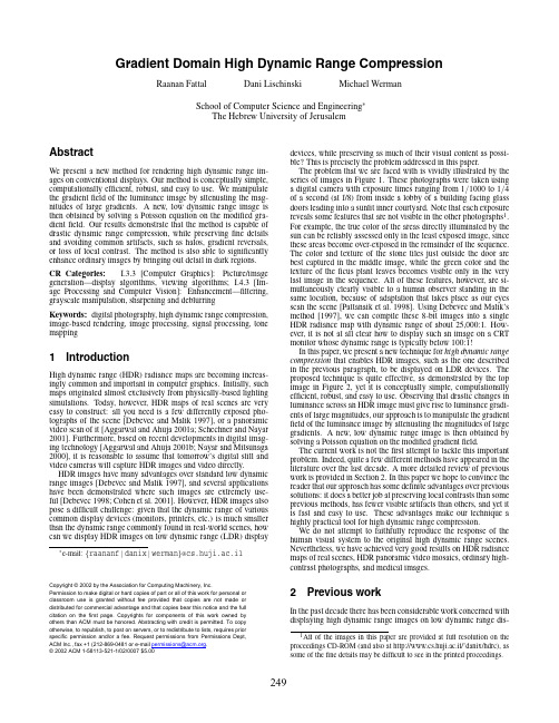
devices, while preserving as much of their visual content as possible? This is precisely the problem addressed in this paper.
The problem that we are faced with is vividly illustrated by the series of images in Figure 1. These photographs were taken using a digital camera with exposure times ranging from 1/1000 to 1/4 of a second (at f/8) from inside a lobby of a building facing glass doors leading into a sunlit inner courtyard. Note that each exposure reveals some features that are not visible in the other photographs1. For example, the true color of the areas directly illuminated by the sun can be reliably assessed only in the least exposed image, since these areas become over-exposed in the remainder of the sequence. The color and texture of the stone tiles just outside the door are best captured in the middle image, while the green color and the texture of the ficus plant leaves becomes visible only in the very last image in the sequence. All of these features, however, are simultaneously clearly visible to a human observer standing in the same location, because of adaptation that takes place as our eyes scan the scene [Pattanaik et al. 1998]. Using Debevec and Malik’s method [1997], we can compile these 8-bit images into a single HDR radiance map with dynamic range of about 25,000:1. However, it is not at all clear how to display such an image on a CRT monitor whose dynamic range is typically below 100:1!
Prevention of Slab Surface Transverse Cracking by Microstructure Control
Schematic illustration of experimental apparatus forsitu solidified hot tensile test.no surrounding tube around the specimen, harmful influ-ence could be neglected. Temperature is measured just above crucible and controlled according to calibration curve measured in advance. Temperature accuracy, stability and distribution were also inspected beforehand. apparatus were placed in a chamber and experiments were carried out in argon atmosphere.kg of steels were melted in a vacuum induction furnace and cast into ingots. The ingots were hot forged and tensile specimens of 10mm diameter were machined from During the experiment, the middle part of the specimen in-situ remelted about 30K above the liquidus. More mm of melting zone, enough for fracture, could be obtained. After 240s holding, the specimens were solidified to 1523K. Then cooling rate is changed tountil test temperature in mild cooling, while it is changed to 20K·sϪ1to 870K, keeping it constant for 120 subsequently reheated up to 1430K at 3.0Kcooled again at 0.4K·sϪ1until test temperature in SSC cooling. After reaching the test temperature and a further holding time of 120s all specimens were deformed until fracture at strain rate of 3.3ϫ10Ϫ4·sϪ1comparable to that during straightening of continuous casting. Reduction of area at fracture and microstructure of specimen are investi-gated. For the purpose of austenite grain size examination, some specimens were kept cooling without deformation. Usual tensile tests without in-situ remelting were also in-vestigated with this apparatus to make a comparison with conventional hot tensile tests. Specimens were reheated up K and held for 240s at which the specimens were never remelted. Other conditions were similar to melted tests.©2.4.Continuous Casting TestEffect of the microstructure on the cracking susceptibili-ty is actually assessed by slab bending tests. Figure 2shows the schematic illustration of the pilot caster used.The caster, which is essentially a vertical, slab-bending de-vice is installed below the pinch rolls. The slabs 150mm thick and 600mm wide were cast at 1.0m/min, standing by in the strand to adjust the surface temperature, then bent at the prescribed surface temperature. All processes were completed within 1200s after casting. Water density of in-tensive cooling zone is altered to control the slab surface microstructure. Slab surface temperature is measured by optical pyrometers set at the bottom of intensive cooling zone and bending zone, which is accompanied by air purge to get rid of water due to mist cooling. Bending radius was 10m and average bending strain and strain rate at the slab surface were estimated as 0.8% and 2ϫ10Ϫ41/s respective-ly, corresponding to those of conventional caster. Surface cracks were detected by using the paint test on a machined surface.3.Results3.1.Ingot Cooling TestFigure 3shows some examples of thermal histories mea-sured from 5mm inside to the ingot surface. Temperature oscillation in each profile is due to intermittent cooling,which controls the cooling rate. In one cooling, the ingot is gradually cooled after withdrawal under mild cooling just as in a conventional continuous casting operation. In other coolings, the ingot is rapidly cooled after withdrawal and subsequently reheated up to 1250K by its own heat capaci-ty. The minimum temperature during the rapid cooling is variously altered and Fig. 3 shows examples of (a) 1050K and (b) 1170K respectively,Figure 4shows microstructures at 5mm inside to the ingot surface. Metallographic examination revealed that the features of microstructures are rather different, though ei-ther fundamental microstructure is ferrite–pearlite. A char-acteristic structure is formed under pattern (a), where sub-stantial volume of ferrite is idiomorph, which seems granu-lar morphology, whereas grain boundary allotriomorph of ferrite is formed under pattern (b) and (c), as conventional-ly produced slabs. In pattern (a), austenite grain boundaries are obscure because there is no ferrite allotriomorphs asso-ciation along the grain. Similar structure is obtained when the minimum temperature during intensive cooling are be-tween 870K and 1050K. As strain concentration at ferrite allotriomorphs cause transverse cracking, reduction of them is expected to prevent cracking. On the other hand, it is conspicuous along grain boundaries under pattern (b) and (c), showing minimum temperature of 1170K during inten-sive cooling, pattern (b), is inadequate for microstructure control. Thus grain boundaries can be easily traced with them, as conventionally produced slabs. In this paper, sec-ondary cooling pattern for microstructure control, which provides momentary intensive cooling until less than 1050K and subsequent reheating is defined as SSC cool-ing.3.2.Hot Tensile TestHot ductility in-situ solidification was plotted in Fig. 5for both cooling patterns. Representative ductility curve as being made up of three regions is obtained under mild cool-ing. SSC cooling, however, gave a significant improvement on the ductility, thus tough embrittlement almost disap-peared. For specimen having low ductility, i.e.RA of Ͻ40%, crack lies within the grain boundary allotriomorphs of ferrite and the fracture mode is intergranular brittle. It is,however, transgranular ductile under SSC cooling, which possesses higher ductility.Microstructure of specimen, which passed through pre-scribed thermal history, however, without strain, is shown in Fig. 6. Prior austenite grain boundary is associated with ferrite allotriomorphs under mild cooling, whereas such ferrite grain could not be seen at austenite grain boundary under SSC cooling corresponding to ingot cooling tests.These results suggest that microstructure control possibly reduces susceptibility to transverse cracking. Further, simi-lar grain size is obtained in the specimen between those coolings.Hot ductility without remelting is plotted in Fig. 7. Hot tensile tests have been generally carried out under reheating process, and clarified that transverse cracking is related©2003ISIJFig.2.Schematic illustration of slab bending test by a pilot con-tinuous caster.Fig.3.Temperature profile for ingot cooling test measured at 5mm inside to the surface.with hot ductility around g –a transformation tempera-ture.1–5)Although precipitates are considered to be resolved during homogenizing treatment during reheating process,present study revealed that the treatment was insufficient to simulate as-cast properties. Remelting prior to deformation is indispensable to evaluate the effect of microstructure on susceptibility to transverse cracking.3.3.Continuous Casting TestSlab surface temperature measured at intensive cooling zone and bending zone is shown in Fig. 8. Although it is difficult to measure them throughout the experiment due to the water drops of mist cooling, those at intensive cooling zone are about 1000K under SSC cooling and 1300K under mild cooling, respectively. Those at bending were1745©2003ISIJMicrostructure of the ingots from 5mm inside to the surface under respective cooling patterns shown in Fig. 3.Arrows in (b) and (c) indicate grain boundary allotriomorph of ferrite.Fig.5.Effect of microstructure control on reduction of area at hot tensile test.Fig.6.Microstructure of the hot ductile specimen without defor-mation under (a) SSC cooling and (b) mild cooling.Arrows in (b) indicate grain boundary allotriomorphs of ferrite.Fig.7.Effect of in-situ remelting and solidification on reduction of area under SSC cooling.about 1070K in both cooling conditions. Thus, the aimed thermal history as examined in ingot-cooling tests and hot tensile tests could be reproduced in continuous casting tests.Summation of transverse cracking length measured on the surface of a half width with 400mm in length is shown in Fig. 9. The transverse cracks take place along the grain boundary under mild cooling, just as in commercial prod-ucts. A number of cracks are found on the surface under mild cooling bent at 1070K. Some cracks still remain even at 1270K despite leaving ductility trough. In contrast, no crack is found under SSC cooling both at 1070K and 1170K bending. Although thermal stress is likely to in-crease according to intensive cooling, the transverse cracks are obviously alleviated by microstructure control, i.e.ap-plying the SSC cooling. Other surface cracking or sub-sur-face cracking is not found under SSC cooling. Moreover,the cracking could be reproduced experimentally despite rather different dimension with a conventional caster.Surface microstructure of these continuously cast slabs were shown in Fig. 10. Idiomorph of ferrite structure is formed under SSC cooling, whereas ferrite allotriomorphs structure associated with austenite grain boundary is formed under mild cooling, corresponding to ingot cooling tests and hot tensile tests. The results proved that suscepti-bility to transverse cracking could be reduced by appropri-ate surface microstructure control by means of secondary cooling in continuous casting strand.Austenite Grain SizeAs fine austenite grain size is well known to alleviate cracking susceptibility, 5–7)those sizes in each cooling con-ditions are examined. However, the microstructure without ferrite allotriomorph association at grain boundary under SSC cooling makes difficult to measure the size. Therefore another ingot cooling tests were conducted, in which the thermal history in the early stage were the same and the cooling rate in the latter half were increased. The operation makes microstructure from ferrite–pearlite to bainite on which austenite grain boundaries are easily observed.Similar experiments under SSC cooling and mild cooling were carried out, and then austenite grain size was exam-ined on cross sections. Austenite grain structure at surface region is shown in Fig. 11. The austenite grain size within mm from surface under SSC cooling is equivalent with that under mild cooling. Therefore, the improvement of hot ductility and prevention of transverse cracking are not a re-sult of austenite grain refinement due to recrystalization.Carbide and/or Nitride PrecipitationMicrographs of carbon extraction replicas from continu-©2003ISIJ8.Surface temperature of continuously cast slabs measured at (a) bottom of intensive cooling zone and (b) bending zone.Fig.9.Influence of thermal history on the slab surface trans-verse cracking investigated by a pilot continuous caster.10.Slab surface microstructure of continuously cast slabsunder (a) SSC cooling and (b) mild cooling. An arrow in (b) indicates grain boundary allotriomorphs of ferrite.11.Austenite grain size of the ingots under (a) SSC coolingand (b) mild cooling.12.Extraction reprica image of fine precipitates at austenitegrain boundary and matrix under (a) SSC cooling and(b) mild cooling.tion under SSC cooling.According to Andrew’s equation,14)A 3transformation temperature is estimated as 1090K. Cracking insensitive microstructure is obtained when minimum temperature dur-ing initial intensive cooling is below this temperature,whereas it is not obtained when minimum temperature does not reach that temperature, as shown in Fig. 4. These results indicate that phase transformation begins during initial in-tensive cooling under SSC cooling.In general, the austenite grain size is refined by recrystal-lization, as commonly applied for mechanical property con-trol of steel. It has been well known that fine austenite grain size bring improvement of hot ductility.5–7)The austenite grain size close to the slab surface under SSC cooling,however, is equivalent with that under mild cooling as shown in Fig. 11. Although measured temperature should involve some error due to dull response and accuracy, these results show that phase transformation has never completed during thermal cycle. That is, the change in the microstruc-ture according to secondary cooling does not originate in the refinement of the austenite grain size by recrystalliza-tion.As the temperature reaches less than A 3temperature dur-ing the thermal cycle, ferrite grain must once begin to pre-cipitate. Such precipitates as (Ti,Nb)(C,simultaneously. Solubility product of TiN, which is most li-able to precipitate among carbide or nitride, in austenite and ferrite phase is expressed as Eqs. (1) and (2), respec-tively.15,16)And they are shown in Fig. 152003ISIJ1748Fig.13.Analysis of grain boundary precipitates under mild cooling by electron diffraction pattern and EDS (a) brightfield image, (b) dark field image, (c) EDS spectra, and (d) schematic representation.14.Analysis of fine precipitates under SSC cooling (a)bright field image and (b) dark field image.Table parison of inter planar spacing.log[Ti%][N%]g ϭϪ14400/T ϩ4.94.........(1)15)log[Ti%][N%]a ϭϪ15960/T ϩ5.79.........(2)16)Substituting the actual content and assuming equilibrium,the initiative of TiN precipitation is estimated at 1583K in austenite phase. Note that solubility product in ferrite phase is one digit smaller than in austenite below A 3temperature.Slab surface transverse cracking is well known to be affect-ed by carbide and/or nitride precipitation. Such precipita-tion at austenite grain boundary or matrix causes strain concentration and low ductility during unbending opera-tion.Behaviour of microstructure and precipitates during SSC cooling and mild cooling is schematically illustrated as shown in Fig. 16. In SSC cooling, ferrite grain must first precipitate during the thermal cycle. When cooling rate is fast enough and sufficient supercooling is achieved, the fer-rite grains precipitate not only at austenite grain boundary but also inside the grain. According to the low solubilityFig.15.Solubility product of TiN in ferrite and austenite calcu-lated by Eqs. (1) and (2).Fig.16.Schematic illustration of mechanism forming mi-crostructure.。
mmcn
A Measurement Study of Peer-to-Peer File Sharing SystemsStefan Saroiu,P.Krishna Gummadi,Steven D.GribbleDept.of Computer Science and Engineering,Univ.of Washington,Seattle,WA,98195-2350ABSTRACTThe popularity of peer-to-peer multimediafile sharing applications such as Gnutella and Napster has created a flurry of recent research activity into peer-to-peer architectures.We believe that the proper evaluation of a peer-to-peer system must take into account the characteristics of the peers that choose to participate.Surprisingly, however,few of the peer-to-peer architectures currently being developed are evaluated with respect to such considerations.In this paper,we remedy this situation by performing a detailed measurement study of the two popular peer-to-peerfile sharing systems,namely Napster and Gnutella.In particular,our measurement study seeks to precisely characterize the population of end-user hosts that participate in these two systems.This characterization includes the bottleneck bandwidths between these hosts and the Internet at large,IP-level latencies to send packets to these hosts,howoften hosts connect and disconnect from the system,howmany files hosts share and download,the degree of cooperation between the hosts,and several correlations between these characteristics.Our measurements showthat there is significant heterogeneity and lack of cooperation across peers participating in these systems.Keywords:Peer-to-Peer,Network Measurements,Wide-Area Systems,Internet Services,Broadband1.INTRODUCTIONThe popularity of peer-to-peerfile sharing applications such as Gnutella and Napster has created aflurry of recent research activity into peer-to-peer architectures.1–6Although the exact definition of“peer-to-peer”is debatable,these systems typically lack dedicated,centralized infrastructure,but rather depend on the voluntary participation of peers to contribute resources out of which the infrastructure is constructed.Membership in a peer-to-peer system is ad-hoc and dynamic:as such,the challenge of such systems is tofigure out a mechanism and architecture for organizing the peers in such a way so that they can cooperate to provide a useful service to the community of users.For example,in afile sharing application,one challenge is organizing peers into a cooperative,global index so that all content can be quickly and efficiently located by any peer in the system.2–4,6 In order to evaluate a proposed peer-to-peer system,the characteristics of the peers that choose to participate in the system must be understood and taken into account.For example,if some peers in afile-sharing system have low-bandwidth,high-latency bottleneck network connections to the Internet,the system must be careful to avoid delegating large or popular portions of the distributed index to those peers,for fear of overwhelming them and making that portion of the index unavailable to other peers.Similarly,the typical duration that peers choose to remain connected to the infrastructure has implications for the degree of redundancy necessary to keep data or index metadata highly available.In short,the system must take into account the suitability of a given peer for a specific task before explicitly or implicitly delegating that task to the peer.Surprisingly,however,few of the architectures currently being developed are evaluated with respect to such considerations.We believe that this is,in part,due to a lack of information about the characteristics of hosts that choose to participate in peer-to-peer systems.We are aware of a single previous study7that measures only one such characteristic,namely the number offiles peers share.In this paper,we remedy this situation by performing a detailed measurement study of the two most popular peer-to-peerfile sharing systems,namely Napster and Gnutella.The hosts that choose to participate in these systems are typically end-users’home or office machines,located at the“edge”of the Internet.Our measurement study seeks to precisely characterize the population of end-user hosts that participate in these two systems.This characterization includes the bottleneck bandwidths between these hosts and the Internet at large,IP-level latencies to send packets to these hosts,howoften hosts connect and disconnect from the system,howmanyfiles hosts share and dow nload,and correlations betw een these characteristics.Our The authors may be contacted at{tzoompy,gummadi,gribble}@measurements—four days for Napster andThere are amount of heterogeneity of sharing vary between three any similar peer-to-peer peers tend to deliberately responsibility depends on peers to tell the truth,or2.METHODOLOGYThe methodology behind our measurements is quite simple.For each of the Napster and Gnutella systems,we proceeded in two steps.First,we periodically crawled each system in order to gather instantaneous snapshots of large subsets of the systems’user population.The information gathered in these snapshots include the IP address and port number of the users’client software,as well as some information about the users as reported by their software.Second,immediately after gathering a snapshot,we actively probed the users in the snapshot over a period of several days to directly measure various properties about them,such as their bottleneck bandwidth.In this section of the paper,wefirst give a brief overview of the architectures of Napster and Gnutella. Following this,we then describe the software infrastructure that we built to gather our measurements,including the Napster crawler,the Gnutella crawler,and the active measurement tools used to probe the users discovered.2.1.The Napster and Gnutella ArchitecturesBoth Napster and Gnutella have similar goals:to facilitate the location and exchange offiles(typically images, audio,or video)amongst a large group of independent users connected through the Internet.In these systems,files are stored on the computers of the individual users or peers,and exchanged through a direct connection between the downloading and uploading peers,over an HTTP-style protocol.All peers in this system are symmetric:they all have the ability to function both as a client and a server.This symmetry distinguishes peer-to-peer systems from many conventional distributed system architectures.Though the process of exchanging files is similar in both systems,Napster and Gnutella differ substantially in howpeers locatefiles(Figure1).In Napster,a large cluster of dedicated central servers maintain an index of thefiles that are currently being shared by active peers.Each peer maintains a connection to one of the central servers,through which thefile location queries are sent.The servers then cooperate to process the query and return a list of matchingfiles and locations.On receiving the results,the peer may choose to initiate afile exchange directly from another peer. In addition to maintaining an index of sharedfiles,the centralized servers also monitor the state of each peer in the system,keeping track of metadata such as the peers’reported connection bandwidth and the duration that the peer has remained connected to the system.This metadata is returned with the results of a query,so that the initiating peer has some information to distinguish possible download sites.There are no centralized servers in Gnutella,however.Instead,Gnutella peers form an overlay network by forging point-to-point connections with a set of neighbors.To locate afile,a peer initiates a controlledflood of the network by sending a query packet to all of its neighbors.Upon receiving a query packet,a peer checks ifany locally storedfiles match the query.If so,the peer sends a query response packet back towards the query originator.Whether or not afile match is found,the peer continues toflood the query through the overlay.To help maintain the overlay as the users enter and leave the system,the Gnutella protocol includes ping and pong messages that help peers to discover other nodes.Pings and pongs behave similarly to query/query-response packets:any peer that sees a ping message sends a pong back towards the originator,and forwards the ping onwards to its own set of neighbors.Ping and query packets thusflood through the network;the scope offlooding is controlled with a time-to-live(TTL)field that is decremented on each hop.Peers occasionally forge newneighbor connections w ith other peers discovered through the ping/pong mechanism.Note that it is possible to have several disjoint Gnutella overlays of Gnutella simultaneously coexisting in the Internet;this contrasts with Napster,in which peers are always connected to the same cluster of central servers.2.2.Crawling the Peer-to-Peer SystemsWe nowdescribe the design and implementation of our Napster and Gnutella craw lers.2.2.1.The Napster CrawlerBecause we did not have direct access to indexes maintained by the central Napster servers,the only way we could discover the set of peers participating in the system at any time was by issuing queries forfiles,and keeping a list of peers referenced in the queries’responses.To discover the largest possible set of peers,we issued queries with the names of popular song artists drawn from a long list downloaded from the web.The Napster server cluster consists of approximately160servers;each peer establishes a connection with only one server.When a peer issues a query,the server the peer is connected tofirst reportsfiles shared by “local users”on the same server,and later reports matchingfiles shared by“remote users”on other servers in the cluster.For each crawl,we established a large number of connections to a single server,and issued many queries in parallel;this reduced the amount of time taken to gather data to3-4minutes per crawl,giving us a nearly instantaneous snapshot of peers connected to that server.For each peer that we discovered during the crawl,we then queried the Napster server to gather the following metadata:(1)the bandwidth of the peer’s connection as reported by the peer herself,(2)the number offiles currently being shared by the peer,(3)the current number of uploads and the number of downloads in progress by the peer,(4)the names and sizes of all thefiles being shared by the peer,and(5)the IP address of the peer.To get an estimate of the fraction of the total user population we captured,we separated the local and remote peers returned in our queries’responses,and compared them to statistics periodically broadcast by the particular Napster server that we queried.From these statistics,we verified that each crawl typically captured between40%and60%of the local peers on the crawled server.Furthermore,this40-60%of the peers that we captured contributed between80-95%of the total(local)files reported to the server.Thus,we feel that our crawler captured a representative and significant fraction of the set of peers.Our crawler did not capture any peers that do not share any of the popular content in our queries.This introduces a bias in our results,particularly in our measurements that report the number offiles being shared by users.However,the statistics reported by the Napster server revealed that the distributions of number of uploads,number of downloads,number offiles shared,and bandwidths reported for all remote users were quite similar to those that we observed from our captured local users.2.2.2.The Gnutella CrawlerThe goal of our Gnutella crawler is the same as our Napster crawler:to gather nearly instantaneous snap-shots of a significant subset of the Gnutella population,as well as metadata about peers in captured subset as reported by the Gnutella system itself.Our crawler exploits the ping/pong messages in the protocol to discover hosts.First,the crawler connects to several well-known,popular peers(such as or ).Then,it begins an iterative process of sending ping messages with large TTLs to known peers,adding newly discovered peers to its list of known peers based on the contents of received pong messages.In addition to the IP address of a peer,each pong message contains metadata about the peer, including the number and total size offiles being shared.We allowed our crawler to continue iterating for approximately two minutes,after which it would typically gather between8,000and10,000unique peers(Figure2).According to measurements reported by Clip2,8this corresponds to at least25%to50%of the total population of peers in the system at any time.After twoFigure2:Number of Gnutella hosts captured by our crawler over timeminutes,we would terminate the crawler,save the crawling results to afile and begin another crawl iteration to gather our next snapshot of the Gnutella population.Unlike our Napster measurements,in which we were more likely to capture hosts sharing popular songs, we have no reason to suspect any bias in our measurements of the Gnutella user population.Furthermore, to ensure that the crawling process does not alter the behavior of the system in any way,our crawler neither forwarded any Gnutella protocol messages nor answered any queries.2.2.3.Crawler StatisticsBoth the Napster and Gnutella crawlers were written in Java,and ran using the IBM Java1.18JRE on Linux 2.2.16.The crawlers ran in parallel on a small number of dual-processor Pentium III700MHz computers with 2GB RAM,and four40GB SCSI disks.Our Napster trace captured four days of activity,from Sunday May 6th,2001through Wednesday May9th,2001.We recorded a total of509,538Napster peers on546,401unique IP addresses.Our Gnutella trace spanned eight days(Sunday May6th,2001through Monday May14th,2001) and captured1,239,487Gnutella peers on1,180,205unique IP-addresses.2.3.Directly Measured Peer CharacteristicsFor each gathered peer population snapshot,we directly measured additional properties of the peers.Our goal was to capture data that would enable us to reason about the fundamental characteristics of the users(both as individuals and as a population)participating in any peer-to-peerfile sharing system.The data collected includes the distributions of bottleneck bandwidths and latencies between peers and our measurement infrastructure, the number of sharedfiles per peer,the distribution of peers across DNS domains,and the“lifetime”of the peers in the system,i.e.,howfrequently peers connect to the systems,and howlong they remain connected.tency MeasurementsGiven the list of peers’IP-addresses obtained by the crawlers,we measured the round-trip latency between the peers and our measurement machines.For this,we used a simple tool that measures the RTT of a40-byte TCP packet exchanged between a peer and our measurement host.Our interest in latencies of the peers is due to the well known feature of TCP congestion control which discriminates againstflows with large round-trip times. This,coupled with the fact that the average size offiles exchanged is in the order of2-4MB,makes latency a very important consideration when selecting amongst multiple peers sharing the samefile.Although we realize that the latency to any particular peer is dependent on the location of the host from which it is measured,we feel the distribution of latencies over the entire population of peers from a given host might be similar(but not identical)from different hosts,and hence,could be of interest.2.3.2.Lifetime MeasurementsTo gather measurements of the lifetime characteristics of peers,we needed a tool that would periodically probea large set of peers from both systems to detect when they were participating in the system.Every peer in bothNapster and Gnutella connects to the system using a unique IP-address/port-number pair;to download afile, peers connect to each other using these pairs.There are therefore three possible states for any participating peer in either Napster or Gnutella:1.offline:the peer is either not connected to the Internet or is not responding to TCP SYN packets becauseit is behind afirewall or NAT proxy.2.inactive:the peer is connected to the Internet and is responding to TCP SYN packets,but it is discon-nected from the peer-to-peer system and hence responds with TCP RST’s.3.active:the peer is actively participating in the peer-to-peer system,and is accepting incoming TCPconnections.We developed a simple tool(which we call LF)using Savage’s“Sting”platform.9To detect the state of a host,LF sends a TCP SYN-packet to the peer and then waits for up to twenty seconds to receive any packets from it.If no packet arrives,we mark the peer as offline.If we receive a TCP RST packet,we mark the peer as inactive.If we receive a TCP SYN/ACK,we label the host as active,and send back a RST packet to terminate the connection.We chose to manipulate TCP packets directly rather than use OS socket calls to achieve greater scalability;this enabled us to monitor the lifetimes of tens of thousands of hosts per workstation.Because we identify a host by its IP address,one limitation in the lifetime characterization of peers our inability of distinguishing hosts sharing dynamic IP addresses(e.g.DHCP).2.3.3.Bottleneck Bandwidth MeasurementsAnother characteristic of peers that we wanted to gather was the speed of their connections to the Internet. This is not a precisely defined concept:the rate at which content can be downloaded from a peer depends on the bottleneck bandwidth between the downloader and the peer,the available bandwidth along the path,and the latency between the peers.The central Napster servers can provide the connection bandwidth of any peer as reported by the peer itself. However,as we will show later,a substantial percentage of the Napster peers(as high as25%)choose not to report their bandwidths.Furthermore,there is a clear incentive for a peer to discourage other peers from downloadingfiles by falsely reporting a low bandwidth.The same incentive to lie exists in Gnutella;in addition to this,in Gnutella,bandwidth is reported only as part of a successful response to a query,so peers that share no data or whose content does not match any queries never report their bandwidths.Because of this,we decided to actively probe the bandwidths of peers.There are two difficult problems with measuring the available bandwidth to and from a large number of hosts:first,available bandwidth can significantlyfluctuate over short periods of time,and second,available bandwidth is determined by measuring the loss rate of an open TCP connection.Instead,we decided to use the bottleneck link bandwidth as afirst-order approximation to the available bandwidth;because our workstations are connected by a gigabit link to the Abilene network,it is likely that the bottleneck link between our workstations and any peer in these systems is last-hop link to the peer itself.This is particularly likely since,as we will show later,most peers are connected to the system using low-speed modems or broadband connections such as cable modems or DSL.Thus,if we could characterize the bottleneck bandwidth between our measurement infrastructure and the peers,we would have a fairly accurate upper bound on the rate at which information could be downloaded from these peers.Bottleneck link bandwidth between two different hosts equals the capacity of the slowest hop along the path between the two hosts.Thus,by definition,bottleneck link bandwidth is a physical property of the network that remains constant over time for an individual path.Although various bottleneck link bandwidth measurement tools are available,10–13for a number of reasons that are beyond the scope of this paper,all of these tools were unsatisfactory for our purposes.Hence,we developed our own tool(called SProbe)14based on the same underlying packet-pair dispersion technique as some of the above-mentioned tools.Unlike other tools,however,SProbe uses tricks inspired by Sting9to actively measure both upstream and downstream bottleneck bandwidths using only a few TCP packets.Our tool also proactively detects cross-traffic that interferes with the accuracy of the packet-pair technique,improving the overall accuracy of our measurements.∗By comparing the reported bandwidths of the peers with our measured ∗For more information about SProbe,refer to .Figure3.Left:CDFs of upstream and downstream bottleneck bandwidths for Gnutella peers;Right:CDFs of down-stream bottleneck bandwidths for Napster and Gnutella peers.bandwidths,we were able to verify the consistency and accuracy of SProbe,as we will demonstrate in Section3.5.2.3.4.A Summary of the Active MeasurementsFor the lifetime measurements,we monitored17,125Gnutella peers over a period of60hours and7,000Napster peers over a period of25hours.For each Gnutella peer,we determined its status(offline,inactive or active) once every seven minutes,and for each Napster peer,once every two minutes.For Gnutella,we attempted to measure bottleneck bandwidths and latencies to a random set of595,974 unique peers(i.e.,unique IP-address/port-number pairs).We were successful in gathering downstream bot-tleneck bandwidth measurements to223,552of these peers,the remainder of which were either offline or had significant cross-traffic.We measured upstream bottleneck bandwidths from16,252of the peers(for various reasons,upstream bottleneck bandwidth measurements from hosts are much harder to obtain than downstream measurements to hosts14).Finally,we were able to measure latency to339,502peers.For Napster,we attempted to measure downstream bottleneck bandwidths to4,079unique peers.We successfully measured2,049peers.In several cases,our active measurements were regarded as intrusive by several monitored systems.Un-fortunately,e-mail complaints received by the computing staffat the University of Washington forced us to prematurely terminate our crawls,hence the lower number of monitored Napster hosts.Nevertheless,we suc-cessfully captured a significant number of data points for us to believe that our results and conclusions are representative for the entire Napster population.3.MEASUREMENT RESULTSOur measurement results are organized according to a number of basic questions addressing the capabilities and behavior of peers.In particular,we attempt to address how many peers are capable of being servers,how many behave like clients,howmany are w illing to cooperate,and also howw ell the Gnutella netw ork behaves in the face of random or malicious failures.3.1.How Many Peers Fit the High-Bandwidth,Low-Latency Profile of a Server?One particularly relevant characteristic of peer-to-peerfile sharing systems is the percentage of peers in the system having server-like characteristics.More specifically,we are interested in understanding what percentage of the participating peers exhibit the server-like characteristics with respect to their bandwidths and latencies. Peers worthy of being servers must have high-bandwidth Internet connections,they should remain highly avail-able,and the latency of access to the peers should generally be low.If there is a high degree of heterogeneity amongst the peers,a well-designed system should pay careful attention to delegating routing and content-serving responsibilities,favoring server-like peers.3.1.1.Downstream and Upstream Measured Bottleneck Link BandwidthsTofit the profile of a high-bandwidth server,a participating peer must have a high upstream bottleneck link bandwidth,since this value determines the rate at which a server can serve content.On the left,Figure3Figure 4.Left:Reported bandwidths For Napster peers;Right:Reported bandwidths for Napster peers,excluding peers that reported “unknown”.presents cumulative distribution functions (CDFs)of upstream and downstream bottleneck bandwidths for Gnutella peers.†From this graph,we see that while 78%of the participating peers have downstream bottleneck bandwidths of at least 100Kbps,only 8%of the peers have upstream bottleneck bandwidths of at least 10Mbps.Moreover,22%of the participating peers have upstream bottleneck bandwidths of 100Kbps or less.Not only are these peers unsuitable to provide content and data,they are particularly susceptible to being swamped by a relatively small number of connections.The left graph in Figure 3reveals asymmetry in the upstream and downstream bottleneck bandwidths of Gnutella peers.On average,a peer tends to have higher downstream than upstream bottleneck bandwidth;this is not surprising,because a large fraction of peers depend on asymmetric links such as ADSL,cable modems or regular modems using the V.90protocol.15Although this asymmetry is beneficial to peers that download content,it is both undesirable and detrimental to peers that serve content:in theory,the download capacity of the system exceeds its upload capacity.We observed a similar asymmetry in the Napster network.The right graph in Figure 3presents CDFs of downstream bottleneck bandwidths for Napster and Gnutella peers.As this graph illustrates,the percentage of Napster users connected with modems (of 64Kbps or less)is about 25%,while the percentage of Gnutella users with similar connectivity is as low as 8%.At the same time,50%of the users in Napster and 60%of the users in Gnutella use broadband connections (Cable,DSL,T1or T3).Furthermore,only about 20%of the users in Napster and 30%of the users in Gnutella have very high bandwidth connections (at least 3Mbps).Overall,Gnutella users on average tend to have higher downstream bottleneck bandwidths than Napster users.Based on our experience,we attribute this difference to two factors:(1)the current flooding-based Gnutella protocol is too high of a burden on low bandwidth connections,discouraging them from participating,and (2)although unverifiable,there is a widespread belief that Gnutella is more popular to technically-savvy users,who tend to have faster Internet connections.3.1.2.Reported Bandwidths for Napster PeersFigure 4illustrates the breakdown of Napster peers with respect to their voluntarily reported bandwidths;the bandwidth that is reported is selected by the user during the installation of the Napster client software.(Peers that report “Unknown”bandwidth have been excluded in the right graph.)As Figure 4shows,a significant percent of the Napster users (22%)report “Unknown”.These users are either unaware of their connection bandwidths,or they have no incentive to accurately report their true bandwidth.Indeed,knowing a peer’s connection speed is more valuable to others rather than to the peer itself;a peer that reports high bandwidth is more likely to receive download requests from other peers,consuming network resources.Thus,users have an incentive to misreport their Internet connection speeds.A well-designed system therefore must either directly measure the bandwidths rather than relying on a user’s input,or create the right†“Upstream”denotes traffic from the peer to the measurement node;“downstream”denotes traffic from the mea-surement node to the peer.Figure 5.Left:Measured latencies to Gnutella peers;Right:Correlation between Gnutella peers’downstream bottleneck bandwidth and latency.incentives for the users to report accurate information to the system.Finally both Figures 3and 4confirm that the most popular forms of Internet access for Napster and Gnutella peers are cable modems and DSLs (bottleneck bandwidths between 1Mbps and 3.5Mbps).3.1.3.Measured Latencies for Gnutella PeersFigure 5(left)shows a CDF of the measured latencies from our measurement nodes to Gnutella peers.Approx-imately 20%of the peers have latencies of at least 280ms,whereas another 20%have latencies of at most 70ms:the closest 20%of the peers are four times closer than the furthest 20%.From this,we can deduce that in a peer-to-peer system where peers’connections are forged in an unstructured,ad-hoc way,a substantial fraction of the connections will suffer from high-latency.On the right,Figure 5shows the correlation between downstream bottleneck bandwidth and the latency of individual Gnutella peers (on a log-log scale).This graph illustrates the presence of two clusters;a smaller one situated at (20-60Kbps,100-1,000ms)and a larger one at over (1,000Kbps,60-300ms).These clusters correspond to the set of modems and broadband connections,respectively.The negatively sloped lower-bound evident in the low-bandwidth region of the graph corresponds to the non-negligible transmission delay of our measurement packets through the low-bandwidth links.An interesting artifact evident in this graph is the presence of two pronounced horizontal bands.These bands correspond to peers situated on the North American East Coast and in Europe,respectively.Although the latencies presented in this graph are relative to our location (Seattle,WA),these results can be extended to conclude that there are three large classes of latencies that a peer interacts with:(1)latencies to peers on the same part of the continent,(2)latencies to peers on the opposite part of a continent and (3)latencies to trans-oceanic peers.As Figure 5shows,the bandwidths of the peers fluctuate significantly within each of these three latency classes.3.2.How Many Peers Fit the High-Availability Profile of a Server?Server worthiness is characterized not only by high-bandwidth and low-latency network connectivity,but also by the availability of the server.If,peers tend to be unavailable frequently,this will have significant implications about the degree of replication necessary to ensure that content is consistently accessible on this system.On the left,Figure 6shows the distribution of uptimes of peers for both Gnutella and Napster.Uptime is measured as the percentage of time that the peer is available and responding to traffic.The “Internet host uptime”curves represent the uptime as measured at the IP-level,i.e.,peers that are in the inactive or active states,as defined in Section 2.3.2.The “Gnutella/Napster host uptime”curves represent the uptime of peers in the active state,and therefore responding to application-level requests.For all curves,we have eliminated peers that had 0%uptime (peers that were never up throughout our lifetime experiment).The IP-level uptime characteristics of peers are quite similar for both systems;this implies that the set of。
毕业设计 英文翻译、译文 一种混沌图像加密并行算法 英译中附英文原文

附件C :译文基于离散混沌映射的图像加密并行算法摘要:最近,针对图像加密提出了多种基于混沌的算法。
然而,它们都无法在并行计算环境中有效工作。
在本文中,我们提出了一个并行图像加密的框架。
基于此框架内,一个使用离散柯尔莫哥洛夫流映射的新算法被提出。
它符合所有并行图像加密算法的要求。
此外,它是安全、快速的。
这些特性使得它是一个很好的基于并行计算平台上的图像加密选择。
1. 介绍最近几年,通过计算机网络尤其是互联网传输的数字图像有了快速增长。
在大 多数情况下,传输通道不够安全以防止恶意用户的非法访问。
因此,数字图像的安全性和隐私性已成为一个重大问题。
许多图像加密方法已经被提出,其中基于混沌的方法是一种很有前途的方向[1-9]。
总的来说,混沌系统具有使其成为密码系统建设中重要组成部分的几个属性:(1)随机性:混沌系统用确定的方法产生长周期、随机的混沌序列。
(2)敏感性:初始值或系统参数的微小差异导致混沌序列的巨大变化。
(3)易用性:简单的公式可以产生复杂的混沌序列。
(4)遍历性:一个混沌状态的变量能够遍历它的相空间里的所有状态,通常这些状态都是均匀分布的。
除了上述性能,有些二维(2D )的混沌映射是图像像素置换天生的优良替代者。
Pichler 和Scharinger 提出一种在扩散操作[1,2]之前使用柯尔莫哥洛夫流映射的图像排列方式。
后来,Fridrich 将此方法扩展到更广义的方式[3]。
陈等人提出基于三维猫映射的图像加密算法[4]l 。
Lian 等人提出基于标准映射的另一种算法[5]。
其实,这些算法在相同的框架下工作:所有的像素在用密码分组链接模式(CBC)模式下的加密之前首先被用离散混沌映射置换,当前像素密文由以前的像素密文影响。
上述过程重复几轮,最后得到加密图像。
这个框架可以非常有效的实现整个图像的扩散。
但是,它是不适合在并行计算环境中运行。
这是因为当前像素的处理无法启动直到前一个像素已加密。
ACM-GIS%202006-A%20Peer-to-Peer%20Spatial%20Cloaking%20Algorithm%20for%20Anonymous%20Location-based%
A Peer-to-Peer Spatial Cloaking Algorithm for AnonymousLocation-based Services∗Chi-Yin Chow Department of Computer Science and Engineering University of Minnesota Minneapolis,MN cchow@ Mohamed F.MokbelDepartment of ComputerScience and EngineeringUniversity of MinnesotaMinneapolis,MNmokbel@Xuan LiuIBM Thomas J.WatsonResearch CenterHawthorne,NYxuanliu@ABSTRACTThis paper tackles a major privacy threat in current location-based services where users have to report their ex-act locations to the database server in order to obtain their desired services.For example,a mobile user asking about her nearest restaurant has to report her exact location.With untrusted service providers,reporting private location in-formation may lead to several privacy threats.In this pa-per,we present a peer-to-peer(P2P)spatial cloaking algo-rithm in which mobile and stationary users can entertain location-based services without revealing their exact loca-tion information.The main idea is that before requesting any location-based service,the mobile user will form a group from her peers via single-hop communication and/or multi-hop routing.Then,the spatial cloaked area is computed as the region that covers the entire group of peers.Two modes of operations are supported within the proposed P2P spa-tial cloaking algorithm,namely,the on-demand mode and the proactive mode.Experimental results show that the P2P spatial cloaking algorithm operated in the on-demand mode has lower communication cost and better quality of services than the proactive mode,but the on-demand incurs longer response time.Categories and Subject Descriptors:H.2.8[Database Applications]:Spatial databases and GISGeneral Terms:Algorithms and Experimentation. Keywords:Mobile computing,location-based services,lo-cation privacy and spatial cloaking.1.INTRODUCTIONThe emergence of state-of-the-art location-detection de-vices,e.g.,cellular phones,global positioning system(GPS) devices,and radio-frequency identification(RFID)chips re-sults in a location-dependent information access paradigm,∗This work is supported in part by the Grants-in-Aid of Re-search,Artistry,and Scholarship,University of Minnesota. Permission to make digital or hard copies of all or part of this work for personal or classroom use is granted without fee provided that copies are not made or distributed for profit or commercial advantage and that copies bear this notice and the full citation on thefirst page.To copy otherwise,to republish,to post on servers or to redistribute to lists,requires prior specific permission and/or a fee.ACM-GIS’06,November10-11,2006,Arlington,Virginia,USA. Copyright2006ACM1-59593-529-0/06/0011...$5.00.known as location-based services(LBS)[30].In LBS,mobile users have the ability to issue location-based queries to the location-based database server.Examples of such queries include“where is my nearest gas station”,“what are the restaurants within one mile of my location”,and“what is the traffic condition within ten minutes of my route”.To get the precise answer of these queries,the user has to pro-vide her exact location information to the database server. With untrustworthy servers,adversaries may access sensi-tive information about specific individuals based on their location information and issued queries.For example,an adversary may check a user’s habit and interest by knowing the places she visits and the time of each visit,or someone can track the locations of his ex-friends.In fact,in many cases,GPS devices have been used in stalking personal lo-cations[12,39].To tackle this major privacy concern,three centralized privacy-preserving frameworks are proposed for LBS[13,14,31],in which a trusted third party is used as a middleware to blur user locations into spatial regions to achieve k-anonymity,i.e.,a user is indistinguishable among other k−1users.The centralized privacy-preserving frame-work possesses the following shortcomings:1)The central-ized trusted third party could be the system bottleneck or single point of failure.2)Since the centralized third party has the complete knowledge of the location information and queries of all users,it may pose a serious privacy threat when the third party is attacked by adversaries.In this paper,we propose a peer-to-peer(P2P)spatial cloaking algorithm.Mobile users adopting the P2P spatial cloaking algorithm can protect their privacy without seeking help from any centralized third party.Other than the short-comings of the centralized approach,our work is also moti-vated by the following facts:1)The computation power and storage capacity of most mobile devices have been improv-ing at a fast pace.2)P2P communication technologies,such as IEEE802.11and Bluetooth,have been widely deployed.3)Many new applications based on P2P information shar-ing have rapidly taken shape,e.g.,cooperative information access[9,32]and P2P spatio-temporal query processing[20, 24].Figure1gives an illustrative example of P2P spatial cloak-ing.The mobile user A wants tofind her nearest gas station while beingfive anonymous,i.e.,the user is indistinguish-able amongfive users.Thus,the mobile user A has to look around andfind other four peers to collaborate as a group. In this example,the four peers are B,C,D,and E.Then, the mobile user A cloaks her exact location into a spatialA B CDEBase Stationregion that covers the entire group of mobile users A ,B ,C ,D ,and E .The mobile user A randomly selects one of the mobile users within the group as an agent .In the ex-ample given in Figure 1,the mobile user D is selected as an agent.Then,the mobile user A sends her query (i.e.,what is the nearest gas station)along with her cloaked spa-tial region to the agent.The agent forwards the query to the location-based database server through a base station.Since the location-based database server processes the query based on the cloaked spatial region,it can only give a list of candidate answers that includes the actual answers and some false positives.After the agent receives the candidate answers,it forwards the candidate answers to the mobile user A .Finally,the mobile user A gets the actual answer by filtering out all the false positives.The proposed P2P spatial cloaking algorithm can operate in two modes:on-demand and proactive .In the on-demand mode,mobile clients execute the cloaking algorithm when they need to access information from the location-based database server.On the other side,in the proactive mode,mobile clients periodically look around to find the desired number of peers.Thus,they can cloak their exact locations into spatial regions whenever they want to retrieve informa-tion from the location-based database server.In general,the contributions of this paper can be summarized as follows:1.We introduce a distributed system architecture for pro-viding anonymous location-based services (LBS)for mobile users.2.We propose the first P2P spatial cloaking algorithm for mobile users to entertain high quality location-based services without compromising their privacy.3.We provide experimental evidence that our proposed algorithm is efficient in terms of the response time,is scalable to large numbers of mobile clients,and is effective as it provides high-quality services for mobile clients without the need of exact location information.The rest of this paper is organized as follows.Section 2highlights the related work.The system model of the P2P spatial cloaking algorithm is presented in Section 3.The P2P spatial cloaking algorithm is described in Section 4.Section 5discusses the integration of the P2P spatial cloak-ing algorithm with privacy-aware location-based database servers.Section 6depicts the experimental evaluation of the P2P spatial cloaking algorithm.Finally,Section 7con-cludes this paper.2.RELATED WORKThe k -anonymity model [37,38]has been widely used in maintaining privacy in databases [5,26,27,28].The main idea is to have each tuple in the table as k -anonymous,i.e.,indistinguishable among other k −1tuples.Although we aim for the similar k -anonymity model for the P2P spatial cloaking algorithm,none of these techniques can be applied to protect user privacy for LBS,mainly for the following four reasons:1)These techniques preserve the privacy of the stored data.In our model,we aim not to store the data at all.Instead,we store perturbed versions of the data.Thus,data privacy is managed before storing the data.2)These approaches protect the data not the queries.In anonymous LBS,we aim to protect the user who issues the query to the location-based database server.For example,a mobile user who wants to ask about her nearest gas station needs to pro-tect her location while the location information of the gas station is not protected.3)These approaches guarantee the k -anonymity for a snapshot of the database.In LBS,the user location is continuously changing.Such dynamic be-havior calls for continuous maintenance of the k -anonymity model.(4)These approaches assume a unified k -anonymity requirement for all the stored records.In our P2P spatial cloaking algorithm,k -anonymity is a user-specified privacy requirement which may have a different value for each user.Motivated by the privacy threats of location-detection de-vices [1,4,6,40],several research efforts are dedicated to protect the locations of mobile users (e.g.,false dummies [23],landmark objects [18],and location perturbation [10,13,14]).The most closed approaches to ours are two centralized spatial cloaking algorithms,namely,the spatio-temporal cloaking [14]and the CliqueCloak algorithm [13],and one decentralized privacy-preserving algorithm [23].The spatio-temporal cloaking algorithm [14]assumes that all users have the same k -anonymity requirements.Furthermore,it lacks the scalability because it deals with each single request of each user individually.The CliqueCloak algorithm [13]as-sumes a different k -anonymity requirement for each user.However,since it has large computation overhead,it is lim-ited to a small k -anonymity requirement,i.e.,k is from 5to 10.A decentralized privacy-preserving algorithm is proposed for LBS [23].The main idea is that the mobile client sends a set of false locations,called dummies ,along with its true location to the location-based database server.However,the disadvantages of using dummies are threefold.First,the user has to generate realistic dummies to pre-vent the adversary from guessing its true location.Second,the location-based database server wastes a lot of resources to process the dummies.Finally,the adversary may esti-mate the user location by using cellular positioning tech-niques [34],e.g.,the time-of-arrival (TOA),the time differ-ence of arrival (TDOA)and the direction of arrival (DOA).Although several existing distributed group formation al-gorithms can be used to find peers in a mobile environment,they are not designed for privacy preserving in LBS.Some algorithms are limited to only finding the neighboring peers,e.g.,lowest-ID [11],largest-connectivity (degree)[33]and mobility-based clustering algorithms [2,25].When a mo-bile user with a strict privacy requirement,i.e.,the value of k −1is larger than the number of neighboring peers,it has to enlist other peers for help via multi-hop routing.Other algorithms do not have this limitation,but they are designed for grouping stable mobile clients together to facil-Location-based Database ServerDatabase ServerDatabase ServerFigure 2:The system architectureitate efficient data replica allocation,e.g.,dynamic connec-tivity based group algorithm [16]and mobility-based clus-tering algorithm,called DRAM [19].Our work is different from these approaches in that we propose a P2P spatial cloaking algorithm that is dedicated for mobile users to dis-cover other k −1peers via single-hop communication and/or via multi-hop routing,in order to preserve user privacy in LBS.3.SYSTEM MODELFigure 2depicts the system architecture for the pro-posed P2P spatial cloaking algorithm which contains two main components:mobile clients and location-based data-base server .Each mobile client has its own privacy profile that specifies its desired level of privacy.A privacy profile includes two parameters,k and A min ,k indicates that the user wants to be k -anonymous,i.e.,indistinguishable among k users,while A min specifies the minimum resolution of the cloaked spatial region.The larger the value of k and A min ,the more strict privacy requirements a user needs.Mobile users have the ability to change their privacy profile at any time.Our employed privacy profile matches the privacy re-quirements of mobiles users as depicted by several social science studies (e.g.,see [4,15,17,22,29]).In this architecture,each mobile user is equipped with two wireless network interface cards;one of them is dedicated to communicate with the location-based database server through the base station,while the other one is devoted to the communication with other peers.A similar multi-interface technique has been used to implement IP multi-homing for stream control transmission protocol (SCTP),in which a machine is installed with multiple network in-terface cards,and each assigned a different IP address [36].Similarly,in mobile P2P cooperation environment,mobile users have a network connection to access information from the server,e.g.,through a wireless modem or a base station,and the mobile users also have the ability to communicate with other peers via a wireless LAN,e.g.,IEEE 802.11or Bluetooth [9,24,32].Furthermore,each mobile client is equipped with a positioning device, e.g.,GPS or sensor-based local positioning systems,to determine its current lo-cation information.4.P2P SPATIAL CLOAKINGIn this section,we present the data structure and the P2P spatial cloaking algorithm.Then,we describe two operation modes of the algorithm:on-demand and proactive .4.1Data StructureThe entire system area is divided into grid.The mobile client communicates with each other to discover other k −1peers,in order to achieve the k -anonymity requirement.TheAlgorithm 1P2P Spatial Cloaking:Request Originator m 1:Function P2PCloaking-Originator (h ,k )2://Phase 1:Peer searching phase 3:The hop distance h is set to h4:The set of discovered peers T is set to {∅},and the number ofdiscovered peers k =|T |=05:while k <k −1do6:Broadcast a FORM GROUP request with the parameter h (Al-gorithm 2gives the response of each peer p that receives this request)7:T is the set of peers that respond back to m by executingAlgorithm 28:k =|T |;9:if k <k −1then 10:if T =T then 11:Suspend the request 12:end if 13:h ←h +1;14:T ←T ;15:end if 16:end while17://Phase 2:Location adjustment phase 18:for all T i ∈T do19:|mT i .p |←the greatest possible distance between m and T i .pby considering the timestamp of T i .p ’s reply and maximum speed20:end for21://Phase 3:Spatial cloaking phase22:Form a group with k −1peers having the smallest |mp |23:h ←the largest hop distance h p of the selected k −1peers 24:Determine a grid area A that covers the entire group 25:if A <A min then26:Extend the area of A till it covers A min 27:end if28:Randomly select a mobile client of the group as an agent 29:Forward the query and A to the agentmobile client can thus blur its exact location into a cloaked spatial region that is the minimum grid area covering the k −1peers and itself,and satisfies A min as well.The grid area is represented by the ID of the left-bottom and right-top cells,i.e.,(l,b )and (r,t ).In addition,each mobile client maintains a parameter h that is the required hop distance of the last peer searching.The initial value of h is equal to one.4.2AlgorithmFigure 3gives a running example for the P2P spatial cloaking algorithm.There are 15mobile clients,m 1to m 15,represented as solid circles.m 8is the request originator,other black circles represent the mobile clients received the request from m 8.The dotted circles represent the commu-nication range of the mobile client,and the arrow represents the movement direction.Algorithms 1and 2give the pseudo code for the request originator (denoted as m )and the re-quest receivers (denoted as p ),respectively.In general,the algorithm consists of the following three phases:Phase 1:Peer searching phase .The request origina-tor m wants to retrieve information from the location-based database server.m first sets h to h ,a set of discovered peers T to {∅}and the number of discovered peers k to zero,i.e.,|T |.(Lines 3to 4in Algorithm 1).Then,m broadcasts a FORM GROUP request along with a message sequence ID and the hop distance h to its neighboring peers (Line 6in Algorithm 1).m listens to the network and waits for the reply from its neighboring peers.Algorithm 2describes how a peer p responds to the FORM GROUP request along with a hop distance h and aFigure3:P2P spatial cloaking algorithm.Algorithm2P2P Spatial Cloaking:Request Receiver p1:Function P2PCloaking-Receiver(h)2://Let r be the request forwarder3:if the request is duplicate then4:Reply r with an ACK message5:return;6:end if7:h p←1;8:if h=1then9:Send the tuple T=<p,(x p,y p),v maxp ,t p,h p>to r10:else11:h←h−1;12:Broadcast a FORM GROUP request with the parameter h 13:T p is the set of peers that respond back to p14:for all T i∈T p do15:T i.h p←T i.h p+1;16:end for17:T p←T p∪{<p,(x p,y p),v maxp ,t p,h p>};18:Send T p back to r19:end ifmessage sequence ID from another peer(denoted as r)that is either the request originator or the forwarder of the re-quest.First,p checks if it is a duplicate request based on the message sequence ID.If it is a duplicate request,it sim-ply replies r with an ACK message without processing the request.Otherwise,p processes the request based on the value of h:Case1:h= 1.p turns in a tuple that contains its ID,current location,maximum movement speed,a timestamp and a hop distance(it is set to one),i.e.,< p,(x p,y p),v max p,t p,h p>,to r(Line9in Algorithm2). Case2:h> 1.p decrements h and broadcasts the FORM GROUP request with the updated h and the origi-nal message sequence ID to its neighboring peers.p keeps listening to the network,until it collects the replies from all its neighboring peers.After that,p increments the h p of each collected tuple,and then it appends its own tuple to the collected tuples T p.Finally,it sends T p back to r (Lines11to18in Algorithm2).After m collects the tuples T from its neighboring peers, if m cannotfind other k−1peers with a hop distance of h,it increments h and re-broadcasts the FORM GROUP request along with a new message sequence ID and h.m repeatedly increments h till itfinds other k−1peers(Lines6to14in Algorithm1).However,if mfinds the same set of peers in two consecutive broadcasts,i.e.,with hop distances h and h+1,there are not enough connected peers for m.Thus, m has to relax its privacy profile,i.e.,use a smaller value of k,or to be suspended for a period of time(Line11in Algorithm1).Figures3(a)and3(b)depict single-hop and multi-hop peer searching in our running example,respectively.In Fig-ure3(a),the request originator,m8,(e.g.,k=5)canfind k−1peers via single-hop communication,so m8sets h=1. Since h=1,its neighboring peers,m5,m6,m7,m9,m10, and m11,will not further broadcast the FORM GROUP re-quest.On the other hand,in Figure3(b),m8does not connect to k−1peers directly,so it has to set h>1.Thus, its neighboring peers,m7,m10,and m11,will broadcast the FORM GROUP request along with a decremented hop dis-tance,i.e.,h=h−1,and the original message sequence ID to their neighboring peers.Phase2:Location adjustment phase.Since the peer keeps moving,we have to capture the movement between the time when the peer sends its tuple and the current time. For each received tuple from a peer p,the request originator, m,determines the greatest possible distance between them by an equation,|mp |=|mp|+(t c−t p)×v max p,where |mp|is the Euclidean distance between m and p at time t p,i.e.,|mp|=(x m−x p)2+(y m−y p)2,t c is the currenttime,t p is the timestamp of the tuple and v maxpis the maximum speed of p(Lines18to20in Algorithm1).In this paper,a conservative approach is used to determine the distance,because we assume that the peer will move with the maximum speed in any direction.If p gives its movement direction,m has the ability to determine a more precise distance between them.Figure3(c)illustrates that,for each discovered peer,the circle represents the largest region where the peer can lo-cate at time t c.The greatest possible distance between the request originator m8and its discovered peer,m5,m6,m7, m9,m10,or m11is represented by a dotted line.For exam-ple,the distance of the line m8m 11is the greatest possible distance between m8and m11at time t c,i.e.,|m8m 11|. Phase3:Spatial cloaking phase.In this phase,the request originator,m,forms a virtual group with the k−1 nearest peers,based on the greatest possible distance be-tween them(Line22in Algorithm1).To adapt to the dynamic network topology and k-anonymity requirement, m sets h to the largest value of h p of the selected k−1 peers(Line15in Algorithm1).Then,m determines the minimum grid area A covering the entire group(Line24in Algorithm1).If the area of A is less than A min,m extends A,until it satisfies A min(Lines25to27in Algorithm1). Figure3(c)gives the k−1nearest peers,m6,m7,m10,and m11to the request originator,m8.For example,the privacy profile of m8is(k=5,A min=20cells),and the required cloaked spatial region of m8is represented by a bold rectan-gle,as depicted in Figure3(d).To issue the query to the location-based database server anonymously,m randomly selects a mobile client in the group as an agent(Line28in Algorithm1).Then,m sendsthe query along with the cloaked spatial region,i.e.,A,to the agent(Line29in Algorithm1).The agent forwards thequery to the location-based database server.After the serverprocesses the query with respect to the cloaked spatial re-gion,it sends a list of candidate answers back to the agent.The agent forwards the candidate answer to m,and then mfilters out the false positives from the candidate answers. 4.3Modes of OperationsThe P2P spatial cloaking algorithm can operate in twomodes,on-demand and proactive.The on-demand mode:The mobile client only executesthe algorithm when it needs to retrieve information from the location-based database server.The algorithm operatedin the on-demand mode generally incurs less communica-tion overhead than the proactive mode,because the mobileclient only executes the algorithm when necessary.However,it suffers from a longer response time than the algorithm op-erated in the proactive mode.The proactive mode:The mobile client adopting theproactive mode periodically executes the algorithm in back-ground.The mobile client can cloak its location into a spa-tial region immediately,once it wants to communicate withthe location-based database server.The proactive mode pro-vides a better response time than the on-demand mode,but it generally incurs higher communication overhead and giveslower quality of service than the on-demand mode.5.ANONYMOUS LOCATION-BASEDSERVICESHaving the spatial cloaked region as an output form Algo-rithm1,the mobile user m sends her request to the location-based server through an agent p that is randomly selected.Existing location-based database servers can support onlyexact point locations rather than cloaked regions.In or-der to be able to work with a spatial region,location-basedservers need to be equipped with a privacy-aware queryprocessor(e.g.,see[29,31]).The main idea of the privacy-aware query processor is to return a list of candidate answerrather than the exact query answer.Then,the mobile user m willfilter the candidate list to eliminate its false positives andfind its exact answer.The tighter the spatial cloaked re-gion,the lower is the size of the candidate answer,and hencethe better is the performance of the privacy-aware query processor.However,tight cloaked regions may represent re-laxed privacy constrained.Thus,a trade-offbetween the user privacy and the quality of service can be achieved[31]. Figure4(a)depicts such scenario by showing the data stored at the server side.There are32target objects,i.e., gas stations,T1to T32represented as black circles,the shaded area represents the spatial cloaked area of the mo-bile client who issued the query.For clarification,the actual mobile client location is plotted in Figure4(a)as a black square inside the cloaked area.However,such information is neither stored at the server side nor revealed to the server. The privacy-aware query processor determines a range that includes all target objects that are possibly contributing to the answer given that the actual location of the mobile client could be anywhere within the shaded area.The range is rep-resented as a bold rectangle,as depicted in Figure4(b).The server sends a list of candidate answers,i.e.,T8,T12,T13, T16,T17,T21,and T22,back to the agent.The agent next for-(a)Server Side(b)Client SideFigure4:Anonymous location-based services wards the candidate answers to the requesting mobile client either through single-hop communication or through multi-hop routing.Finally,the mobile client can get the actualanswer,i.e.,T13,byfiltering out the false positives from thecandidate answers.The algorithmic details of the privacy-aware query proces-sor is beyond the scope of this paper.Interested readers are referred to[31]for more details.6.EXPERIMENTAL RESULTSIn this section,we evaluate and compare the scalabilityand efficiency of the P2P spatial cloaking algorithm in boththe on-demand and proactive modes with respect to the av-erage response time per query,the average number of mes-sages per query,and the size of the returned candidate an-swers from the location-based database server.The queryresponse time in the on-demand mode is defined as the timeelapsed between a mobile client starting to search k−1peersand receiving the candidate answers from the agent.On theother hand,the query response time in the proactive mode is defined as the time elapsed between a mobile client startingto forward its query along with the cloaked spatial regionto the agent and receiving the candidate answers from theagent.The simulation model is implemented in C++usingCSIM[35].In all the experiments in this section,we consider an in-dividual random walk model that is based on“random way-point”model[7,8].At the beginning,the mobile clientsare randomly distributed in a spatial space of1,000×1,000square meters,in which a uniform grid structure of100×100cells is constructed.Each mobile client randomly chooses itsown destination in the space with a randomly determined speed s from a uniform distribution U(v min,v max).When the mobile client reaches the destination,it comes to a stand-still for one second to determine its next destination.Afterthat,the mobile client moves towards its new destinationwith another speed.All the mobile clients repeat this move-ment behavior during the simulation.The time interval be-tween two consecutive queries generated by a mobile client follows an exponential distribution with a mean of ten sec-onds.All the experiments consider one half-duplex wirelesschannel for a mobile client to communicate with its peers with a total bandwidth of2Mbps and a transmission range of250meters.When a mobile client wants to communicate with other peers or the location-based database server,it has to wait if the requested channel is busy.In the simulated mobile environment,there is a centralized location-based database server,and one wireless communication channel between the location-based database server and the mobile。
Lower bounds on the efficiency of generic cryptographic constructions
Informally, we say a one-way (trapdoor) permutation π : {0, 1} n → {0, 1}n has security S if any circuit of size at most S inverts π with probability less than 1/S (one can think of S as a slightly super-polynomial function of n but our results hold for any choice of S ). Given this definition, our results may be summarized as follows. Pseudorandom generators (PRGs). Let U denote the uniform distribution over -bit strings. A PRG is a deterministic, length-increasing function G : {0, 1} → {0, 1} +k such that G(U ) is computationally indistinguishable (by poly-time algorithms) from U +k . The notion of a PRG was introduced by Blum and Micali [8] and Yao [42], who showed that PRGs can be constructed from any one-way permutation. (This was subsequently improved by H˚ astad, et al. [27], who show that a PRG can be constructed from any one-way function.) Their construction, using a later improvement of Goldreich and Levin [22] (see also [18, Section 2.5.3]), requires Θ(k/ log S ) invocations of a one-way permutation with security S in order to construct a PRG stretching its input by k bits. This is the best known efficiency for generic constructions (i.e., constructions based on an arbitrary one-way permutation). We show that this is essentially the best efficiency that can be obtained using generic constructions. More formally, we show that any (black-box) generic construction of a PRG that stretches its input by k bits while making fewer than Ω(k/ log S ) invocations of a one-way permutation with security S implies the unconditional existence of a PRG (i.e., without any invocations of the one-way permutation). Put another way, the only way to come up with a more efficient construction of a PRG is to design a PRG from scratch! This would in particular imply the unconditional existence of a one-way function, as well as a proof that P = N P . (Families of ) universal one-way hash functions (UOWHFs). A UOWHF H = {h s } is a family of length-decreasing functions (all defined over the same domain and range) such that for any input x and random choice of h i ∈ H it is hard to find a collision (i.e., a y = x such that hi (y ) = hi (x)). UOWHFs were introduced by Naor and Yung [36], who 2
Scrambling adversarial errors using few random bits
Scrambling Adversarial Errors Using Few Random Bits,Optimal Information Reconciliation,and Better Private CodesAdam Smith∗Weizmann Institute of Scienceadam.smith@weizmann.ac.ilJanuary23,2006AbstractWhen communicating over a noisy channel,it is typically much easier to deal with random, independent errors with a known distribution than with adversarial errors.This paper looks athow one can use schemes designed for random errors in an adversarial context,at the cost ofrelatively few additional random bits and without using unproven computational assumptions.The basic approach is to permute the positions of a bit string using a permutation drawn from a t-wise independent family,where t=o(n).This leads to two new results:•We construct computationally efficient information reconciliation protocols correcting pnadversarial binary Hamming errors with optimal communication and entropy loss n(h(p)+o(1))bits,where n is the length of the strings and h()is the binary entropy function.Information reconciliation protocols are important tools for dealing with noisy secrets incryptography;they are also used to synchronize remote copies of largefiles.•We improve the randomness complexity(key length)of efficiently decodable capacity-approaching private codes fromΘ(n log n)to n+o(n).We also present a simplified proof of an existential result on private codes due to Langberg(FOCS’04).1Introduction1.1Partially Dependent ErrorsSuppose Alice sends n bits to Bob over a binary channel,and at mostτ=pn of them areflipped.A code C:{0,1}k→{0,1}n can correct all such corruptions if and only if the Hamming distance between any two codewords(points in the image)is at least2τ+1.There are proven limits on how well such codes can perform,and known codes which can be decoded in polynomial time perform even more poorly.In contrast,codes which correct random errors(say,where each bit isflipped independently with probability p,or where a random subset of pn bits isflipped)perform much better:there are explicit,polynomial-time decodable codes which transmit at rates arbitrarily close to the Shannon capacity1−h(p).1This is typically a factor of2greater than existential upper bounds on the performance of codes for adversarial errors;the advantage over known,polynomial-time decodable codes is even greater.∗Supported by the Louis L.and Anita M.Perlman Postdoctoral Fellowship.1The function h()is the binary entropy function h(p)=−p lg p−(1−p)lg(1−p).All logarithms in this paper are base2.We show that for concatenated codes[For66],which can correct random errors at transmission rates arbitrarily close to the Shannon capacity,decoding continues to work with high probability even when the errors are only(almost)t-wise independent for t=o(n).In other words,for this class of codes,the errors need only be slightly random in order to achieve rate close to1−h(p) (the entropy of an almost t-wise independent error distribution can be as low as O(t)).The proof consists of re-analyzing the performance of concatenated codes using bounds on sums of partially dependent random variables.This observation leads to a general strategy for dealing with an adversarial channel,assuming –crucially–that the errors introduced by the adversary are independent of Alice’s random coins. We will see two settings in which this assumption is justified:information reconciliation and a class of private codes.The general approach is:1.Alice chooses at random a permutationπ:[n]→[n](where[n]={1,...,n}from a family ofpermutations which is t-wise independent,meaning that the images of any t indices i1,...,i t∈[n]look like a sample of t points chosen uniformly without replacement from[n].Such permutations can be chosen using only O(t log n)random bits(Kaplan,Naor and Reingold [KNR05])2.We refer to the algorithm mapping seeds to permutations as the KNR generator.2.Alice now encodes her message m using a concatenated code C with rate close to capacity,permutes the bits of C(m)using the inverseπ−1.We abuse notation and denote the permuted string byπ−1(C(m)).She sendsπ−1(C(m))through the channel to Bob.3.Bob can‘unpermute’the corrupted word which he received by applyingπ(this assumes thatAlice can somehow send Bob the short description ofπ).Bob ends up with C(m),corrupted in a set of positions which was chosen(almost)t-wise independently.That is,if the adversary added an error vector e∈{0,1}n,the code is faced with decoding the error vectorπ(e).By the result mentioned above,the code C will correct the errors introduced by the adversary with high probability,and Bob can learn the original message m.The idea of permuting a string to randomize errors and thus reach capacity is by no means new.However,previous approaches require choosing,and sending or storing,a fully random permutation[BBR88](this requiresΘ(n log n)random bits)or assume the existence of a pseudo-random generator[Lip94,DGL04].Our approach can be seen as a derandomization of the generic approach,replacing a cryptographic pseudo-random generator based on a hardness assumption with a specific,combinatorial generator tailored to this application.We now explain two applications of this idea in more detail.1.2Information ReconciliationSuppose that Alice and Bob share an n-bit secret string.Alice’s copy w of the shared string is slightly different from Bob’s copy w .Alice would like to send a short message S(w)to Bob which allows him to correct the errors in w (and thus recover w)whenever w and w differ in at most τbits.The randomized map S()that Alice applies to w is called a non-interactive information reconciliation scheme,or simply a sketch,correctingτbinary Hamming errors.3A typical example of a sketch isS(w)=syn C(w),where syn C is the syndrome of a linear error-correcting code C with block length n[BBR88].(The syndrome is the linear map given by the parity check matrix of the code.)If C has dimension 2The constructions of[KNR05]only produce almost t-wise independent permutations.See Section3.2for details.3This is a different use of the term“sketch”than one sometimes sees in the algorithms literature,where it means, roughly,a short string allowing one to estimate distances between a particular vector and other points.k,then syn C(w)is only n−k bits long.If the minimum distance of C is at least2τ+1,then syn C(w)allows Bob to correct anyτerrors in w .Moreover,the correction process is efficient (polynomial-time)if one can correctτchannel errors using the code in polynomial time.Formally,a sketch consists of two(randomized)algorithms“sketch”(S:{0,1}n→{0,1} )and “recover”(Rec:{0,1}n×{0,1} →{0,1}n).The parameter is called the length of the sketch.Definition1.A sketch correctsτadversarial errors with probability1− if for all pairs w,w ∈{0,1}n which differ in at mostτpositions,Rec(w ,S(w))=w with probability at least1− over the random coins of S and Rec.No guarantee is provided about the output of Rec when the distance between w and w is more thanτ.Also,we assume that w is chosen before the value S(w)(that is,the pair w,w is independent of the coins of S(w)).Sketches are useful for cryptographic settings where secrets may be subject to noise,such as when keys come from biometrics or other measurements[JW99,JS02,DRS04,BDK+05],quantum cryptography[BBR88,BBCM95,BS93],Maurer’s bounded storage model[Din05,DS05],and several variants on settings with correlated randomness,e.g.[RW04,RW05].4They have also been consideredin communication complexity,e.g.[Orl92,Orl93,CPSV00,MT02,MTZ03].We focus here on the length of the sketch:how many bits must Alice send to Bob?When wis drawn uniformly from{0,1}n,at least nh(p)(1−o(1))bits are necessary if the scheme correctsτ=pn errors:S(w)allows Bob to distinguish w from all other strings at distance pn from w ,thatis from about2nh(p)candidates.The same bound applies to the entropy loss of the sketch,which we discuss at the end of this section.Techniques from previous work allow one to construct several protocols matching this bound[BBR88, Lip94,DGL04,Gur03,DRS04,RW05].The results are not stated explicitly in the form that interests us;in Section3.1we cast them in the setting of reconciliation protocols and compare the parameters they achieve.To our knowledge,all of them either•work only for a known distribution on the error vector w⊕w (typically,the errors are assumed to be independent),•require an exponential-time computation on Bob’s part to recover w,or•assume the existence of pseudo-random generators.The general approach of the previous section yields thefirst sketch for binary strings which solves all the problems above:the sketch has length n(h(p)+o(1)),makes no assumptions on the distribution of the pair w,w except that the Hamming distance dist(w,w )is bounded,allows Bob to recover w with all but negligible probability in polynomial time,and requires no unproven computational assumptions.Here we give a high-level description:Protocol1.Given a parameterδ>0:(Step1)Alice chooses a permutationπwhich is almost t-wise independent for t=δn/log(n). Using the KNR permutation generator,this takes only O(t log n)=O(δn)bits.(Step2)Alice permutes the bits of w usingπ−1(the inverse is for technical reasons),and encodes the result using 4In some of these settings,Bob is simply Alice at a later point in time.The sketch is“transmitted”by storingit–and so having the sketch be non-interactive is important.Nevertheless,the lower bound of nh(p)discussed belowon the communication complexity and entropy loss of sketches applies equally well to interactive schemes,so the protocols we discuss are optimal even if interaction is possible.There are some reconciliation settings,not directly relevant to our discussion,where interaction is known to help;see,for example,the work of Orlitsky[Orl90].the concatenated code C described above which has rate (1−h (p )−δ)and efficiently corrects any t -wise independent error distribution.(Step 3)Alice sendsS (w )=description of π O (δn )bits ,syn C (π(w )) n (h (p )+δ)bits.This sketch corrects pn errors with probability 1−exp(Ω(δ3n/log n )),as long as δis not too small (larger than some constant times loglog n/√log n ).See Section 3.2for a precise analysis.The Relation to Entropy Loss In cryptographic settings,a sketch is usually used as the first step of a protocol,following which Alice and Bob derive a shared,secret key from w .Suppose that Eve is tapping the line and trying to learn as much as possible.The most important parameter of a sketch is then the entropy loss of the scheme.Entropy loss can be defined in several ways (see,e.g.,[DRS04,RW05])but in all cases it can be interpreted as the amount of “information,”in bits,revealed about w by S (w ).Typical proofs of security bound the entropy loss of a scheme simply by bounding the number of bits sent from Alice to Bob which depend on the message w .5This suffices as a definition of entropy loss for our purposes.We refer the reader to [DRS04,RW05]for discussions of the correct general definition.The lower bound of n (h (p )−o (1))applies to the entropy loss as well as the length of a sketch (again,by considering the special case of random,independent errors).Since the length of a sketch provides an upper bound on its entropy loss,communication-optimal sketches are also optimal for entropy loss.Nevertheless,some sketches from previous work are optimal for entropy loss but not communication,and so we include entropy loss as a separate entry in our comparison of various protocols (Table 1in Section 3.1).1.3Private CodesPrivate codes were named and first studied explicitly by Langberg [Lan04],with the goal of commu-nicating at the Shannon capacity even in the face of adversarial errors.The idea is that if Alice and Bob share a key ahead of time —secret from the adversary controlling the channel—then they can send information at a higher rate than they could by using a standard code.Definition 2.An adversarial channel introducing pn errors is a randomized map N :{0,1}n →{0,1}n such that for all inputs w ,the distance dist (w,N (w ))is at most pn with probability 1.Definition 3.A [n,k, key ]private code is a pair of algorithms P C,D ,where P C :{0,1}k ×{0,1} key →{0,1}n and D :{0,1}n ×{0,1} key →{0,1}k .The private code corrects pn errors with probability 1− if for all messages x ∈{0,1}k and for all adversarial channels N introducing at most pn errors,the probability over r that D (N (P C (x ;r ));r )=x is at least 1− .The private code is efficient if both P C and D run in polynomial time.Efficient Private Codes For any p ∈(0,1),there are efficient private codes which achieve capacity,in the sense that they correct pn errors with high probability and transmit a message of k ≈n (1−h (p ))bits.The rate is optimal since sharing a secret key does not increase the capacity of a binary symmetric channel,and a private code must,in particular,correct binary symmetric errors with high probability.A construction of such private codes is implicit in [DGL04]and described in detail in [Lan04].The scheme has key length key =Θ(n log n ),since the key contains a uniformly random permutation5There are exceptions.For example,the analysis of the code-offset scheme for non-linear codes in [DRS04]does not have so simple a form,but no instances are known where the generality of non-linear codes is useful.of [n ].The general strategy described in Section 1.1applies here:the uniform random permutation can be replaced by an almost t -wise independent permutation,reducing the key length from n log n to n +o (n ).We obtain the following protocol:Protocol 2.Given a shared key (a,s ),where a ∈{0,1}n ,s ∈{0,1}δn :(Step 1)Alice runs KNR generator with t =δn/log n on seed s to obtain a permutation πs :[n ]→[n ].(Step 2)Alice encodes x using the concatenated code C of Section 1.1for partially dependent errors.(Step 3)Alice sends:P C (x ;a,s )=π−1s (C (x ))⊕a.To decode the received string y ,Bob runs the decoder for C on π(y )⊕a .The scheme corrects pn adversarial errors with error =exp(−Ω(δ3n/log n ).The idea of the analysis is that the mask a eliminates all dependency between the errors in the channel and the permutation πs ,and thus we can apply the general approach from Section 1.1.See Section 4for a precise analysis and a comparison to parameters achieved in previous work.Inefficient Schemes Based on List-Decoding For any p ∈(0,1),there exist private codes which correct pn errors,transmit a message of k ≈n (1−h (p ))bits,and use a very short secret key:only 4log n +2log 1 bits (Langberg,[Lan04]).This amount of randomness is optimal up to constant factors [Lan04].In Appendix A,we present a simplified proof of Langberg’s result,based on a cryptographic intuition.Roughly:given a good list decodable code LDC ,and a message authentication scheme (MAC),Alice can use the shared randomness as the MAC key and send the encoding of the original message x together with the tag given by the MAC:P C (x ;r )=LDC (x,mac (x ;r )).Incorrect decoding is roughly equivalent to a forged MAC tag,which occurs with very low prob-ability.The problem with this construction is that it is not computationally efficient.The scheme relies on the existence of a good list-decodable code but,as discussed in Section 3.1,polynomial-time list-decodable codes that approach capacity are only known in the extreme ranges of p (p ≈0or p ≈12).The scheme of Protocol 2is,surprisingly,the best known (capacity-achieving)private code with efficient decoding.1.4Organization of this PaperSection 2presents a family of capacity-approaching concatenated codes and shows that t -wise independence of the errors is sufficient to guarantee correct decoding with high probability.Section 3of the paper discusses communication-optimal reconciliation schemes.We first discuss protocols which follow directly from ideas in previous work (Section 3.1),and then analyze the performance of Protocol 1(Theorem 4).Finally,Section 4we look at the application to private codes (Theorem 5).Langberg’s existential construction of good private codes can be found in Appendix A.2Codes for Partially Dependent ErrorsDefinition 4.A random variable E =(E 1,...,E n )on {0,1}n is t -wise independent of weight pnif for any set I ={i 1,...,i t }of t indices in [n ],the restriction E |I def =(E i 1,...,E i t )has statisticaldistance at most 2−t from the distribution it would have if E was chosen uniformly from the set of binary vectors with exactly pn ones.We say a code C corrects an error distribution E with probability 1− if there is a decoding algorithm Dec such that,for all messages m ,the probability over E that Dec (C (m )⊕E )=m is at least 1− .6Theorem 1.For any δ=Ω(log log n/√log n ),there is a family of linear concatenated codes oflength n and rate R =1−h (p )−δwhich corrects all t -wise independent error distributions of weight pn with probability 1−2−Ω(δ2t )as long as ω(log n )<t <δn/10.We will typically set t =δn/log n ,in which case the error probability of the decoding scales as 2−Ω(δ3n/log n ).2.1Underlying Concatenated CodeThe code construction has two parameters:the block size b in bits,which is at most O (log n ),and the overhead δ,which determines the rate R =n (1−h (p )−δ).The block length will ultimately be set to about log 1δ /δ2,although we will leave it as an explicit parameter to make the construction easier to follow.Inner Code:a linear code of block length b and rate R 0=1−h (p )−δ/2which corrects random errors with probability µ=2−Ω(δ2b ).We will later choose b large enough so that µ≤δ/10.This code is a linear code selected by exhaustive search (see details below).It can be decoded in time poly(2b )=poly(n ).Outer Code:A linear code with length n 1=n/b and rate R 1=1−δ/2over an alphabet of size2R 0b ,which corrects Ω(δn )adversarial errors in polynomial time.For concreteness,say the code corrects δn 1/5errors.We can use a Reed-Solomon or algebraic-geometric code (details below).These codes can be decoded in time O (n 3)and even,in some cases,in time O (n polylog n ).The final code is the concatenation of the codes above:the message is first encoded with the outer code,and then each of the symbols is encoded with the inner code.The final block length is n =n 1b ,and the final rate is R 0R 1≥1−h (p )−δ,as desired.By a line of analysis due to Forney [For66],and which is now standard,this code will correct random,independent errors well.The decoder simply attempts to correct errors in each of the blocks separately,by exhaustive search.Each block corrects all of its errors with probability 1−µ,where µ=2−Ω(δ2b ).The outcome of the decoding operation within each block is independent of all the other blocks,and so with overwhelming probability,the number of incorrectly decoded blocks is at most,say,2µn 1.The decoder then concatenates the resulting messages and attempts to decode the result using the outer code.We chose µ<δ/10and so the high probability bound on the number of bad blocks,2µn 1,is at most the error-correction threshold of the outer code,δn 1/5.As long as the 2µn 1bound is not exceeded,the outer code corrects all the blocks which decoded incorrectly in the first phase,and recovers the original message.The overall decoding error of this process is 2−Ω(δ2n ).Note that this is the simplest approach to decoding a concatenated code (it is called hard decoding ),but it is sufficient for our purposes since we do not attempt to optimize the constants in the exponent.We now give more detailed information on the component codes of this construction.6Note that for linear codes,the quantification over m is unimportant since the code is invariant under translation;we can typically assume that C (m )=0n without loss of generality.Inner code details:Random linear codes.For any 1,R0,p,and for sufficiently large b, there exists a linear code with block length b and rate R0=1−h(p)−ρwhich corrects binary symmetric errors withflip parameter p with error probability at most2−ρ2b/3.Such a code can be found with high probability in time poly(2b).The code can be encoded in time b2and decoded in time2b(h(p)+ρ)by exhaustive search.For an analysis of the performance of random coding,see,e.g.,[CT91].The extension to linear codes follows by noting that pairwise independence of the codewords is sufficient for the proofs to work,and the running time of code construction comes from considering a2b-size subclass of linear codes such as Wozencraft codes[vL92].Outer code details:RS and AG codes For any length n,dimension k≤n and prime power alphabet size q>n,Reed-Solomon codes are poly-time constructible and decodable[n,k,d]q codes with distance d=n−k+1.For any length n,dimension k≤n and(possibly very small)alphabet size q which is a prime power squared,there exists a poly-time constructible and decodable family of[n,k,d]q codes with d≥n−k−n√q−1+1.See[vL92,Sti93]for details.If the dimension R0b is of the inner code is large enough(at least log(n1)),then one can use a Reed-Solomon code,which correctsδn1/4errors.When b is smaller,one may use analgebraic-geometric code,which corrects14·n1(δ−1/√2R0b)errors(we need to round R0b toan even integer,but this is not a problem as it is at least some large constant).We will later set b so that the number of corrected errors is at leastδn1/5.2.2Code Performance with Partially Dependent ErrorsWe now prove that the hard decoding algorithm mentioned above performs well even when the errors are only t-wise independent.The main tool is a Chernoff-like bound on a sum of almost t-wise independent variables.Suppose we have events denoted by binary random variables X1,...,X n such that every subset of t of the events is close to independent,in the sense that the probability that they occur simultaneously is not too high.Then the sum of those variables is tightly concentrated about its mean.The bound we use here is due to Schmidt et al.[SSS95,Eqn.(2)].It also appears in Ding et al.[DHRS04,Lemma5.9].Fact2([SSS95,DHRS04]).Suppose X1,...,X n are binary random variables,each with expectationat mostµ,such that for every set of t indices i1,...,i t,we have Pr[X i1=···X it=1]≤2µt.Thenfor B>1,the probability that the sum ni=1X i exceeds Bµn is at most2B−tµn−t.Let E be any t-wise independent error distribution of weightτn,as in Definition4.We will need two claims relating the performance on E to the case of independent errors:Lemma3.1.In each block,the probability of a decoding error with errors from E is at most twice theprobability of a decoding error with random independent errors.Consequently,each block is wrong with probability at mostµ=2−Ω(δ2b).2.For any subset of t/b of the blocks,the probability over E that a decoding mistake occurssimultaneously in all blocks is at most2µt/b.Wefirst use the lemma to prove Theorem1,and then give the proof of the lemma.Proof of Theorem1.Let X1,...,X n1be binary random variables which indicate whether a decod-ing error occurred in each of the blocks.By part(1)of the lemma,the expectation of X i is at mostµ.Now look at any subset of t =t/b blocks.By part (2)of the lemma,the probability that all X i ’s in that set occur simultaneously is at most 2µt .Thus,the X i ’s satisfy the conditions of the tail bound above (Fact 2)with parameters n 1,t and µ.We are interested in the probability that more than δn 1/5errors occur,so B =δ/(5µ).The probability of a global decoding error is at most 2 δ5µ−t/b µn 1 −t/b .When t <δn/10,this is at most 2 10µδ t/b .Recall that µ,the probability of a mistake in each block,is 2−Ω(δ2b ).By making b sufficiently large (a constant times log 1δ /δ2),the fraction µ/δis dominated by the block decoding error µ,and so the global decoding error is at most 2−Ω(δ2t ),as desired.Since we assumed that δ=Ω(loglog n/√log n ),the block length b is always O (log n )and so decoding can always be done in polynomialtime.Remark 2.1.The constants in the proof above are fairly easy to calculate.A random linear code of length b and rate 1−h (p )−ρcorrects random,independent errors with probability at least 1−2−ρ2b/3.Going through the proof above,one gets that b should be about 24log 1δ /δ2,and theglobal decoding error is bounded above by 2−δ2t/24.♦Proof of Lemma 3.Part 1:Let D 1be the distribution on {0,1}b obtained by flipping b coins independently with probability p of outcome 1.Let D 2be the distribution on {0,1}b obtained by randomly selecting a substring of exactly b bits from a string of n bits containing pn ones.We can think of D 1as sampling b positions with replacement from the same string as D 2;the distributions are equal conditioned on D 1never having a collision (i.e.sampling the same position twice).A collision occurs with probability at most b 2/n ,which tends to 0since b =O (log n ).Let S ⊆{0,1}b be the set of errors that are incorrectly decoded by a particular linear code.Pr(D 2∈S )=Pr(D 1∈S |no collision)≤Pr(D 1∈S )Pr(no collision)≤Pr(D 1∈S )1−o (1)We are in fact concerned with the performance of the code on a particular subset of b positions from the random vector E .By definition,these have statistical difference at most 2−t from D 2.Since t >b ,this is much smaller than the probability of a decoding error under D 1or D 2(which are both 2−Ω(δ2b )).Overall,moving from independent errors to errors from E costs a factor of at most 2in the probability of a decoding mistake.Part 2:Consider any t/b blocks.These involve t bits from E ,which are close to an “ideal”distribution —a sample of exactly t positions from a string of n bits with pn ones.Consider what happens under this ideal distribution when we decode the inner code using the maximum likelihood algorithm,which outputs the codeword closest to the received word.The probability of correct decoding then decreases monotonically with the number of bits flipped in a particular block.When we condition on the event that a decoding mistake occurs in block 1,the probability of a decoding mistake then goes down in all other blocks,since fewer bits are likely to be flipped there.Similarly,conditioning on decoding mistakes happening simultaneously in any i blocks makes a decoding mistake of any other block less likely.The probability that t/b blocks simultaneously make mistakes is thus at most µt/b under the ideal distribution (recall µis the mistake probability in each block).If we consider now what happens under the distribution E ,the probability of simultaneous decoding mistakes is at most µt/b +2−t (by the Definition 4).Finally,since µ>2−b ,we can bound the mistake probability by 2µt/b ,asdesired.3Communication-Optimal Information Reconciliation 3.1Optimal Reconciliation Protocols Using Previous WorkAs mentioned in the introduction,several communication-optimal reconciliation protocols can be derived directly using ideas from the literature.None of the protocols appears explicitly in theform that interests us and so,in this section,we translate the relevant work to our setting.Table 1states the parameters and basic properties of various protocols.As a point of comparison we also include a protocol based on the syndrome of a standard linear code lying on the Gilbert-Varshamov bound (this corresponds to the best existential results on such codes).Reducing Random to Worst-Case Errors Assume,for a moment,that the differences between w and w are somehow guaranteed to be random and independent.We could then match the nh (p )lower bound efficiently by using the syndrome syn C of a polynomial-time decodable code which achieves the Shannon capacity on a binary symmetric channel (e.g.the concatenated code of Section 2.1).The code has dimension n (1−h (p )−o (1)),and so the sketch is only n (h (p )+o (1))bits long.Of course,we want to avoid such a strong assumption.In all of the settings where sketches are used,it makes sense to minimize the requirements on the exact stochastic properties of the noise process being dealt with.For example,it is easy to estimate the number of errors introduced by some particular noise process,but it is difficult,in general,to estimate the precise distribution on the errors,or even to test if it satisfies specific “target”properties such as independence.Con-sider,for example,biometric data.Their binary representations are typically the result of several transformations of the original non-binary data.Close inputs (say,iris scans)may well correspond to close binary strings,but there is no reason to suppose errors in different parts of the string representation would be independent.A natural way around this is for Alice to choose a random permutation π:[n ]→[n ](here[n ]={1,...,n })and use it to permute the bits of w (Bennett et al.[BBR88,p.216]).She sends the pair π,syn C (π(w ))to Bob,who computes syn C (π(w ))and XORs this with the received string to obtain syn C (π(w ⊕w )).Now the distribution on π(w ⊕w )depends only on the distance between w and w .If it is at most pn ,then running the syndrome decoding algorithm on syn C (π(w )⊕π(w ))will recover the error vector w ⊕w with high probability.7The problem is that this scheme requires a lot of communication since the description of πis n log n bits.The next natural step is to use a cryptographic pseudo-random generator to choose π,and send only the seed of the generator instead of an explicit description of π(this idea is implicit in,for example,[DGL04]).This reduces the total communication to only n (h (p )+o (1)),but requires an unproven hardness assumption.How,then,can we get around this?A first observation is that this solution does not require the adversary introducing the errors to be computationally bounded;instead,it relies on the fact that the decoding algorithm for the code is polynomial time.The adversary’s strategy is limited to the choice of w and w and so she can always be described by a circuit of size 2n .The class of tests which the generator must fool is given by applying the syndrome decoder for C to syn C (π(w ⊕w ))and checking if the result is indeed w ⊕w .Since we have some control over the choice of the code C ,the problem begins to look more like a classical,algorithmic de-randomization question:how many random bits are necessary to fool the decoder for C on all inputs?Protocol 1and our analysis of concatenated codes show that o (n )bits are sufficient.Removing the assumption of a7We are in fact using the code to correct errors which are not independent,but rather chosen randomly conditioned on exactly a certain number of errors occurring.It is not difficult to see that concatenated codes correct such errors with high probability,e.g.by tracing through the argument of Section 2.1.More generally,say a decoder is monotone if for every error pattern e which it correctly repairs,it also correctly repairs all error patterns which are subsets of e .(Since we deal with linear codes it is sufficient to talk about the error pattern,not the actual corrupted word).Then restricting oneself to uniformly random errors of weight τ≤pn can increase the mistake probability of the code by at most a factor O (√n )since (1)the worst case occurs with exactly pn errors and (2)such strings occupy a Ω(1/√n )fraction of the binary symmetric distribution.The hard decoder for concatenated codes may not always be monotone,but the fraction of errors on which it behaves monotonically is high enough for the same argument to work.。
- 1、下载文档前请自行甄别文档内容的完整性,平台不提供额外的编辑、内容补充、找答案等附加服务。
- 2、"仅部分预览"的文档,不可在线预览部分如存在完整性等问题,可反馈申请退款(可完整预览的文档不适用该条件!)。
- 3、如文档侵犯您的权益,请联系客服反馈,我们会尽快为您处理(人工客服工作时间:9:00-18:30)。
Can Heterogeneity Make Gnutella Scalable?Qin Lv(qlv@)Sylvia Ratnasamy(sylviar@)Scott Shenker(shenker@)1IntroductionEven though recent research has identified many differ-ent uses for peer-to-peer(P2P)architectures,file shar-ing remains the dominant(by far)P2P application on the Internet.Despite various legal problems,the num-ber of users participating in thesefile-sharing systems, and number offiles transferred,continues to grow at a remarkable pace.File-sharing applications are thus be-coming an increasingly important feature of the Internet landscape and,as such,the scalability of these P2P sys-tems is of paramount concern.While the peer-to-peer nature of data storage and data transfer in these systems is inherently scalable,the scalability offile location and query resolution is much more problematic.The earliest P2Pfile-sharing systems(e.g.,Napster, Scour)relied on a centralized directory to locatefiles. While this was sufficient for the early days of P2P,it is clearly not a scalable architecture.These centralized-directory systems were followed by a number of fully decentralized systems such as Gnutella and Kazaa. These systems form an overlay network in which each P2P node“connects”to several other nodes.These P2P systems are unstructured in that the overlay topology is ad hoc and the placement of data is completely unre-lated to the overlay topology.Searching on such net-works essentially amounts to random search,in which various nodes are probed and asked if they have any files matching the query;one can’t do better on such unstructured systems because there is no information about which nodes are likely to have the relevantfiles. P2P systems differ in how they construct the overlay topology and how they distribute queries.Gnutella,for example,floods all queries and uses a TTL to restrict the scope of theflood.The advantage of such unstruc-tured systems is that they can easily accommodate a highly transient node population.The disadvantage is that it is hard tofind the desiredfiles without distribut-ing queries widely.It seemed clear,at least in the academic research community,that such random search methods were in-herently unscalable.As a result,a number of research groups have proposed designs for what we call“highly structured”P2P systems[9,13,10,15].In these struc-tured systems the overlay topology is tightly controlled andfiles(or pointers tofiles)are placed at precisely specified locations.1These highly structured systems provide a mapping between thefile identifier and loca-tion,so that queries can be efficiently routed to the node with the desiredfile(or,again,the pointer to the desired file).These systems thus offer a very scalable solution for“exact-match”queries.2However,structured designs are likely to be less re-silient in the face of a very transient user population, precisely because it is hard to maintain the structure (such as neighbor lists,etc.)required for routing to function efficiently when nodes are joining and leav-ing at a high rate.Moreover,it has yet to be demon-strated that these structured systems,while well-suited for exact-match queries,can scalably implement a full range of partial query techniques,such as keyword searching,which are common on currentfile-sharing systems.3Despite these issues,wefirmly believe in the value of these structured P2P systems,and have actively partic-ipated in their design.However,the(sometimes unspo-ken)motivating assumption behind much of the work on structured P2P systems is that unstructured P2P sys-tems such as Gnutella are inherently not scalable,and therefore should be abandoned.Our goal in this work is to revisit that motivating assumption and ask if Gnutella (and systems like it)could be made more scalable.Wedo so because,if scalability concerns were removed,these unstructured P2P systems might be the preferredchoice forfile-sharing and other applications with thefollowing characteristics:keyword searching is the common operation,most content is typically replicated at a fair frac-tion of participating sites,andthe node population is highly transientThefirst condition is that one often doesn’t know theexactfile identifier,or is looking for a set offiles allmatching a given attribute(e.g.,all by the same artist).The second is that one isn’t typically searching for ex-tremely rarefiles that are only stored at a few nodes.This would apply to the music-sharing that dominatestoday’sfile-sharing systems.The third condition seemsto apply to currently popular P2P systems,although itmay not apply to smaller community-based systems.File-sharing is one(widely deployed)example thatfits these criteria,distributed search engines[4]mightwell be another.Unstructured P2P systems may be asuitable choice for these applications because of theiroverall simplicity and their ability to tolerate tran-sient user populations and comfortably support key-word searches.4This all depends,of course,on whetheror not such systems can be made scalable,and that isthe question we address in this short paper.Our approach to improving the scalability of thesesystems is based on recent work which shows the preva-lence of heterogeneity in deployed P2P systems and onwork improving the efficiency of search in unstructurednetworks.After reviewing this relevant background inSection2,we describe,in Section3,a simpleflow con-trol algorithm that takes advantage of heterogeneity andevaluate its performance in Section4.We offer thisalgorithm not as a polished design but as a proof-of-concept that heterogeneity can be used to improve thescalability of unstructured P2P systems.Similarly,oneshould take this position paper not as a“proof”thatGnutella can be made scalable,but as a conjecture insearch of more evidence.5Power-law random graphs are graphs where the degree distri-bution is a power-law and the nodes are connected randomly con-sistent with the degree distribution.A node’s“degree”is its numberof neighbors.6With proactive replication,an object may be replicated at anode even though that node has not requested the object.Passivereplication,where nodes hold copies only if they’ve requested theobject,is the standard approach in Gnutella-like P2P systems.graphs as a given and instead ask how to best searchon them.They,too,suggest the use of random walks,but that these random walks should be biased to seekout high-degree nodes.They show how this leads tosuperior scaling behavior in the limit of large systems.However,their work does not take into account thequery load on individual nodes;as shown by[8]thehigh-degree nodes carry an extremely large share of thequery traffic and are likely to be overloaded.Heterogeneity:Saroiu et al.,in[11],report on the re-sults of a measurement study of Napster and Gnutella.Their study reveals(amongst other things)a significantamount of heterogeneity in bandwidth across peers.The authors of[11]argue that architectures for P2Psystems should take into account the characteristics ofparticipating hosts,including their heterogeneity.How-ever,since the measurement study was the main focusof[11],they did not propose any design strategies.These two lines of work,the observed heterogene-ity and the improvements to Gnutella-like P2P systems,lead us to the following ing random-walk searches on power-law random graphs is an effi-cient search technique,but results in a very skewed us-age pattern with some nodes carrying too large a shareof the load.Measurement studies reveal,however,thatnode capabilities(particularly in terms of bandwidth,but presumably in terms of other resources such asCPU,memory and disk)are also skewed.If we couldalign these two skews–that is,have the highest capac-ity nodes carry the heaviest burdens–we might end upwith a scalable P2P design.This is what we attempt to do in the next section.3DesignOur design for an unstructured P2P system uses a dis-tributedflow control and topology construction algo-rithm that(1)restricts theflow of queries into each nodeso they don’t become overloaded and(2)dynamicallyevolves the overlay topology so that queriesflow to-wards the nodes that have sufficient capacity to han-dle them.7Over this capacity-driven topology we usea biased random walk quite similar to that employedin[1].The combination of these algorithms results ina system where queries are directed to high capacity8represents node’s current spare capacity.Withthe above bounds on and,a node can atmost increase its current outgoing rate to by an amount equal tonode’s current spare capacity.recvSlowDown(node,node)//node receives a slowdown message fromFigure1:Pseudo-code forflow control and topology adaptation.Although not explicitly shown in the pseu-docode,the upper bound on outMax is enforced in per-forming the increase operations on outMax.gets the overloaded node(node)out of the way.If the overloaded node cannotfind an appropriate neighbor (as would be the case when all of’s neighbors are running close to capacity),it requests node to throt-tle the number of queries it is forwarding to node(i.e. reduce outMax[p,i]).The detailed pseudocode for the above high-level description is shown in Figure1. Note that allflow control/topology adjustment deci-sions made by a node are based on local information (i.e.about the node itself and its neighbors).Further, if a node’s capacity was to undergo a sudden change or if the node leaves the system,the topology would auto-matically re-adapt to accommodate the change.Our simulations in Section4use the algorithm from Figure1with parameter values of,, and.9We defer an exploration of the pa-rameter space to later work.While our initial simula-tion results appear promising,we expect to incorporate extensions and modifications to the above rules as we continue to study the behavior of our algorithm.For10With state-keeping,a search is given a unique identifier.A node then remembers the neighbors to which it has already for-warded queries for a given identifier,and if a query with the same identifier arrives back at the node,it is forwarded to a different ing state-keeping thus reduces the likelihood that a random walk will traverse the same path twice.State can be dis-carded after a short time by a node,so it does not become burden-some.010********607005101520253035404550a v g #h o p s#queries performed (x 12000)Chang of avg #hops: alpha = 2.0, avg replic ratio = 1%10000-node graph204060801001248163264128256512p e r c e n t a g e o f q u e r i e s f i n i s h e d (%)#hopsCumulative Hop Distribution: alpha = 2.0, avg replic ratio = 1%last 12000 queries1101001000110100100010000n o d e d e g r e enode rankDegree Distribution: alpha = 2.0, avg replic ratio = 1%10000-node random graphFigure 2:Degree distribution,average query resolution time and the distribution of query resolution times for a 10,000node simulation using a Zipf-like capacity distribution Simulation methodology:We use,as our main eval-uation metric,the average query resolution time (as measured in terms of the number of application-level hops required to find a particular object).We measure this in simulations in which the object popularity,the rate at which queries are issued for it,follows a Zipf-like distribution where the popularity of the ’th most popular object is proportional to .In these simu-lations we used (based on the Gnutella mea-surements in [12]).Individual nodes generate queries using a Poisson process with an average query rate of 1.2queries/minute.Recall,as described above,that we use a proportional replication strategy so that objects are replicated proportional to their query rate.The av-erage degree of replication is 1%11–that is,on average objects are replicated on 1%of the nodes,but the more popular objects are replicated more than the less popu-lar ones.Recall also that objects are assigned randomly to nodes,proportional to their capacity .To investigate the effect of heterogeneous node ca-pabilities,we use two different capacity distributions.First,we use a Zipf-like distribution where is propor-tional to where .Second,we used a distri-bution based (loosely)on the measured bandwidth dis-tributions of [11].Here,we assume 5capacity levels separated by an order of magnitude.The node pop-ulation is then divided amongst these levels as shown in Table 1.The distribution reflects the observation that a fair fraction of Gnutella clients have dial-up con-nections to the Internet,the majority are connected via cable-modem or DSL and a small number of partici-pants,via high speed lines.For each simulation,we start with nodes connectedPercentage of nodesx45%100x4.9%10000x010********607005101520253035404550a v g #h o p s#queries performed (x 12000)Chang of avg #hops: Gnutella, avg replic ratio = 1%5000-node graph204060801001248163264128256512p e r c e n t a g e o f q u e r i e s f i n i s h e d (%)#hopsCumulative Hop Distribution: Gnutella, avg replic ratio = 1%last 10000 queries11010012level 3level 4level 5n o d e d e g r e enode resource levelDegree Distribution: Gnutella, avg replic ratio = 1%5000-node graphFigure 3:Degree distribution,average query resolution time and the distribution of query resolution times for a 5,000node simulation using a Gnutella-like capacity distribution In [7]the authors propose a cluster-based architec-ture for P2P systems (CAP).CAP organizes nodes into a two-level hierarchy using a centralized cluster-ing server [6].Each cluster has a delegate node that acts as directory server for objects stored by nodes within the cluster.Delegate nodes perform intra-cluster node membership registration while a central server tracks existing clusters and their delegates.To some extent,our algorithms achieve the same effect as CAP,with high capacity nodes behaving like delegate nodes.There are however significant differences:unlike CAP our algorithms are completely decentralized and we do not build an explicit hierarchy.File sharing in FreeNet [2]uses hints about the place-ment of files to improve search scalability.FreeNet does not address node heterogeneity.6DiscussionWe started this paper with the basic question of whether one could make unstructured P2P systems scalable.Building on the work in [8,3,1,11]we proposed a de-sign that appears to achieve significant scalability.This design is extremely preliminary,and and our evaluation leaves many questions unanswered.We offer it how-ever,merely as support for the conjecture that unstruc-tured P2P systems can be significantly improved,per-haps to the point where their scalability is no longer a barrier.Our design also raised the more philosophical ques-tion of how to deal with heterogeneity.Most of the highly structured P2P designs start with the assumption of a homogeneous node population and then alter their designs to accommodate heterogeneity.The design we present here actively exploits heterogeneity.One can ask whether the highly structured designs could also be modified to exploit heterogeneity.References[1]A DAMIC ,L.,H UBERMAN ,B.,L UKOSE ,R.,AND P UNIYANI ,A.Search in power law net-works.Physical Review.E 64(2001),46135–46143.[2]C LARKE ,I.,S ANDBERG ,O.,W ILEY ,B.,AND H ONG ,T.Freenet:A Distributed AnonymousInformation Storage and Retrieval System.ICSI Workshop on Design Issues in Anonymity and Unobservability,July 2000.[3]C OHEN ,E.,ANDS HENKER ,S.Optimal replication in random search networks.preprint,2001.[4]I NFRASEARCH ..[5]K A Z A A..[6]K RISHNAMURTHY , B.,AND W ANG ,J.On network-aware clustering of web clients.InProceedings of SIGCOMM ’00(Stockholm,Sweden,Aug.2000).[7]K RISHNAMURTHY ,B.,W ANG ,J.,AND X IE ,Y.Early measurements of a cluster-based archi-tecture for p2p systems.In ACM SIGCOMM Internet Measurement Workshop (San Francisco,Nov.2001).[8]L V ,C.,C AO ,P.,C OHEN ,E.,L I ,K.,AND S HENKER ,S.Search and replication in unstruc-tured peer-to-peer networks.preprint,2001.[9]R ATNASAMY ,S.,F RANCIS ,P.,H ANDLEY ,M.,K ARP ,R.,AND S HENKER ,S.A ScalableContent-Addressable Network.In Proceedings of SIGCOMM 2001(Aug.2001).[10]R OWSTRON ,A.,AND D RUSCHEL ,P.Storage management and caching in PAST,a large-scale,persistent peer-to-peer storage utility.In Proceedings of the Eighteenth SOSP (2001),ACM.[11]S AROIU ,S.,G UMMADI ,K.,AND G RIBBLE ,S.A measurement study of peer-to-peer filesharing systems.In Proceedings of Multimedia Conferencing and Networking (San Jose,Jan.2002).[12]S RIPANIDKULCHAI ,K.The popularity of gnutella queries and its implications on scalability.In O’Reilly’s (Feb.2001).[13]S TOICA ,I.,M ORRIS ,R.,K ARGER ,D.,K AASHOEK ,M.F.,AND B ALAKRISHNAN ,H.Chord:A scalable peer-to-peer lookup service for internet applications.In Proceedings of SIGCOMM 2001(Aug.2001).[14]W ITTEN ,I.H.,M OFFAT ,A.,AND B ELL ,T.C.Managing Gigabytes:Compressing andIndexing Documents and Images ,second ed.Morgan Kaufmann,1999.[15]Z HAO ,B.,K UBIATOWICZ ,J.,AND J OSEPH ,A.Tapestry:An infrastructure for fault-tolerantwide-area location and routing.UCB Technical Report,2001.。