二维插值
二维插值算法原理

二维插值算法原理二维插值算法是一种在二维空间中根据已知的数据点来估计未知位置上的数值的算法。
它广泛应用于图像处理、地理信息系统和数值模拟等领域。
其原理是基于数学上的连续性和局部平滑性假设,通过利用已知数据点的信息,对未知位置上的数值进行估计。
二维插值算法的基本思想是根据已知的数据点的数值和位置,构建出一个合适的数学模型。
对于每一个未知位置,通过模型可以预测其数值。
这个模型常常是一个多项式函数或者其它形式的连续函数,以便于能够在整个二维空间中插值。
其中最常见的二维插值算法是双线性插值。
双线性插值法假设每个未知位置上的数值都是由其相邻四个已知点的数值线性插值得到的。
具体而言,假设已知的四个点为A、B、C、D,它们的数值分别为f(A)、f(B)、f(C)、f(D)。
对于未知位置P,可以通过以下公式计算得到其数值f(P):f(P) = (1 - u)(1 - v) f(A) + u(1 - v) f(B) + (1 - u)v f(C) + uv f(D)其中,u和v是分别表示未知位置在水平和垂直方向上的相对位置的权重。
这种方法实现简单,计算效率高,可以较为准确地插值出未知位置上的数值。
除了双线性插值之外,还有其它一些更复杂的二维插值算法,如三次样条插值、Kriging插值等。
这些算法在不同的应用场景下具有不同的优势。
例如,三次样条插值在处理光滑函数时效果较好,而Kriging插值则适用于处理具有空间相关性的数据。
选择适合的插值算法可以提高插值结果的质量。
在实际应用中,二维插值算法在处理图像、地理数据和模拟结果等方面具有重要意义。
通过插值算法,可以将有限的离散数据转换为连续的函数,从而对未知位置上的数值进行预测和分析。
同时,它也为数据的可视化提供了基础,使得我们能够更直观地理解数据的分布和变化规律。
总之,二维插值算法是一种有指导意义的数学工具,它通过在二维空间中根据有限的已知数据点估计未知位置上的数值。
matlab中二维插值函数用法

matlab中二维插值函数用法Matlab是一种强大的数学软件,可以对数据进行各种操作和分析。
在Matlab 中,二维插值函数是一种非常常用的工具,它可以帮助我们在已知数据点的基础上,估计其它位置的数值。
在本文中,我们将一步一步介绍二维插值函数的用法,希望对你有所帮助。
首先,我们需要明确一点,二维插值是用于处理二维平面上的数据,即x和y坐标都是变化的。
插值的目的是在这样的二维数据上,估计其它位置的数值,使得整个平面上的数值分布更加密集。
在Matlab中,二维插值函数主要是interp2函数。
该函数的基本语法如下:Vq = interp2(X, Y, V, Xq, Yq, method)其中,X和Y是已知数据点的x和y坐标,V是对应的数值;Xq和Yq是我们要估计数值的位置,Vq是估计得到的数值;method是插值方法,可以是‘linear’、‘nearest’、‘spline’等。
接下来,我们来演示一个具体的例子,以说明interp2函数的用法。
假设我们有一组二维数据如下:X = [1, 2, 3; 1, 2, 3; 1, 2, 3]Y = [1, 1, 1; 2, 2, 2; 3, 3, 3]V = [0, 1, 0; 1, 4, 1; 0, 1, 0]这里,X和Y分别是数据点的x和y坐标,V是对应的数值。
现在我们想要在位置(1.5, 1.5)处进行插值,估计其数值。
我们可以使用interp2函数来完成这个任务:Vq = interp2(X, Y, V, 1.5, 1.5, 'linear')这里,我们使用了‘linear’插值方法,得到的估计值Vq为2。
这就是在位置(1.5, 1.5)处的估计数值。
除了‘linear’插值方法,我们还可以尝试其它方法,比如‘nearest’和‘spline’。
这些方法在实际应用中有着不同的特点,需要根据具体情况选择合适的方法。
例如,‘nearest’方法会选择最近的数据点的数值作为估计值,‘spline’方法则会使用样条插值进行估计。
深入理解插值与卷积,1维插值,2维插值
a = 0.25 (a~c)
a = 1 (d~f)
a = 1.75 (g~i)
a = 0.5(j~l)
不同的a取值对于三次插值的效果。
•16.3.3 二维插值 •基本思想:先在某一维上进行一维插值,然后对这个中间结果的另外 一维进行一维插值。 •二维最近邻插值 •通过对x和y坐标分别取整,可以得到举例给定的连续点(x0,y0)最近的像 •素。
•16.3.2 以卷积方式描述插值 •对连续信号的重建可以描述为线性卷积运算。一般地,可以将插值表达 为给定离散函数g(u)和一连续插值内核w(x)的线性卷积。
• 可以理解为对离散函数的线性求和。 • 一维最近邻内插的插值内核为:
Байду номын сангаас
•线性插值的插值内核为:
最近邻插值(a-c)
线性插值(d-f)
•立方插值的插值内核为:
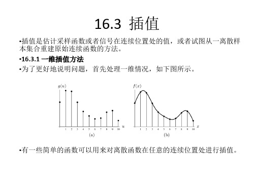
16.3 插值
•插值是估计采样函数或者信号在连续位置处的值,或者试图从一离散样 本集合重建原始连续函数的方法。 •16.3.1 一维插值方法 •为了更好地说明问题,首先处理一维情况,如下图所示。
•有一些简单的函数可以用来对离散函数在任意的连续位置处进行插值。
•最近邻插值 •将连续坐标x近似为最近的整数值u0,并且用样本值g(u0)作为估计的函 数值。下图(a)为其示例。
•线性插值 •连续坐标x的估计值为最近两个样本g(u0)和g(u0+1)的加权求和的形式。 •下图(b)是其示例。
•数值计算中的三次Hermite插值 •给定离散点处的导数值和离散点处的函数值,可以在该离散点之间进行 插值,从而得到一个分段插值函数。该函数满足c1连续。这种插值方式 称为Hermite插值。以多项式构造插值函数则该多项式最多为3次。 •将该多项式写为 • f(x) =ax3 +bx2 + cx + d •例:求离散点0和离散点1之间的插值函数值: •1:约束条件 • f(0)= d; f(1)= a + b + c + d; • f’(0)=c; f’(1)=3a + 2b + c •2:求解上述四个方程,可以得到a,b,c,d的值从而求得插值函数 •三次插值(立方插值) •三次插值(立方插值)与Hermite插值之间的差别在于离散点处的导数 •值并不是事先已知的,而是通过相邻离散点之间的差分得到,如下式所 示 •f‘(0) = α[f(1)-f(-1)],f'(1) = α[f(2)-f(0)] •在上式中α是参数, α控制边缘处的锐化程度。当α =0.5时该插值又称为 •Catmull-Rom插值。
matlab中二维插值函数
matlab中二维插值函数Matlab中的二维插值函数是一种用于在给定有限数据点的情况下估算未知数据点的方法。
它可以用于图像处理、数据分析、数值计算等多个领域。
本文将介绍Matlab中常用的二维插值函数及其应用。
Matlab中的二维插值函数包括interp2、griddata和scatteredInterpolant等。
这些函数可以根据给定的数据点和相应的值,生成一个二维插值函数对象。
通过该对象,可以对未知数据点进行插值计算。
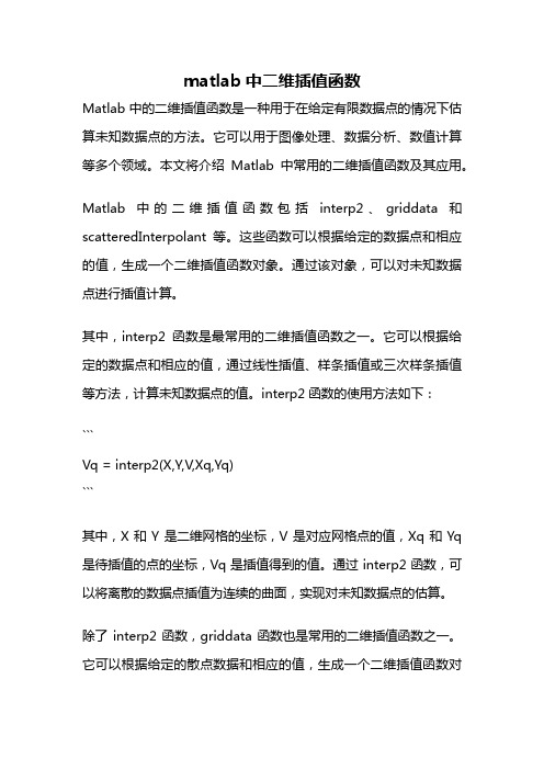
其中,interp2函数是最常用的二维插值函数之一。
它可以根据给定的数据点和相应的值,通过线性插值、样条插值或三次样条插值等方法,计算未知数据点的值。
interp2函数的使用方法如下:```Vq = interp2(X,Y,V,Xq,Yq)```其中,X和Y是二维网格的坐标,V是对应网格点的值,Xq和Yq 是待插值的点的坐标,Vq是插值得到的值。
通过interp2函数,可以将离散的数据点插值为连续的曲面,实现对未知数据点的估算。
除了interp2函数,griddata函数也是常用的二维插值函数之一。
它可以根据给定的散点数据和相应的值,生成一个二维插值函数对象。
griddata函数的使用方法如下:```F = griddata(x,y,v,xq,yq)```其中,x和y是散点数据的坐标,v是对应散点数据的值,xq和yq 是待插值的点的坐标,F是插值得到的函数对象。
通过griddata函数,可以实现对离散数据点的插值计算。
scatteredInterpolant函数也是常用的二维插值函数之一。
它可以根据给定的散点数据和相应的值,生成一个二维插值函数对象。
scatteredInterpolant函数的使用方法如下:```F = scatteredInterpolant(x,y,v)```其中,x和y是散点数据的坐标,v是对应散点数据的值,F是插值得到的函数对象。
通过scatteredInterpolant函数,可以实现对散点数据的插值计算。
griddata二维插值
griddata⼆维插值 对某些设备或测量仪器来说,采集的数据点的位置不是规则排列的⽹格结构(可参考),对于这种数据⽤散点图(每个采样点具有不同的值或权重)不能很好的展⽰其内部结构,因此需要对其进⾏插值,⽣成⼀个规则的栅格图像。
可采⽤griddata函数对已知的数据点进⾏插值,数据点(X, Y)不要求规则排列。
下图分别使⽤Nearest、Linear、Cubic三种插值⽅法对数据点进⾏插值。
插值算法都要⾸先⾯对⼀个共同的问题—— 邻近点的选择(利⽤靠近插值点附近的多个邻近点,构造插值函数计算插值点的函数值)。
应尽可能使所选择的邻近点均匀地分布在待估点周围。
因为使⽤适量的已知点对于插值的精度很重要,当已知点过多时,会使插值准确率下降,因为过多的信息量会掩盖有⽤的信息;被选择的邻近点构成的点分布不均匀,若某个⽅位上的数据点过多,或点集的某些数据点位置较集中,或者数据点过远,都会带来较⼤的插值误差。
griddata函数内部会先对已知的数据点进⾏Delaunay三⾓剖分,当完成三⾓剖分完成后,根据每个三⾓⽚顶点的数值,就可以对三⾓形区域内任意点进⾏线性插值(参考LinearNDInterpolator函数)。
对三⾓⽚内的插值点可采⽤质⼼插值,即是对插值点只考虑与该点最邻近周围点的影响,确定出插值点与最邻近的周围点之相互位置关系,求出与周围点的影响权重因⼦,以此建⽴线性插值公式(参考)。
"""Simple N-D interpolation.. versionadded:: 0.9"""## Copyright (C) Pauli Virtanen, 2010.## Distributed under the same BSD license as Scipy.### Note: this file should be run through the Mako template engine before# feeding it to Cython.## Run ``generate_qhull.py`` to regenerate the ``qhull.c`` file#cimport cythonfrom libc.float cimport DBL_EPSILONfrom libc.math cimport fabs, sqrtimport numpy as npimport scipy.spatial.qhull as qhullcimport scipy.spatial.qhull as qhullimport warnings#------------------------------------------------------------------------------# Numpy etc.#------------------------------------------------------------------------------cdef extern from"numpy/ndarrayobject.h":cdef enum:NPY_MAXDIMSctypedef fused double_or_complex:doubledouble complex#------------------------------------------------------------------------------# Interpolator base class#------------------------------------------------------------------------------class NDInterpolatorBase(object):"""Common routines for interpolators... versionadded:: 0.9"""def__init__(self, points, values, fill_value=np.nan, ndim=None,rescale=False, need_contiguous=True, need_values=True):"""Check shape of points and values arrays, and reshape values to(npoints, nvalues). Ensure the `points` and values arrays areC-contiguous, and of correct type."""if isinstance(points, qhull.Delaunay):# Precomputed triangulation was passed inif rescale:raise ValueError("Rescaling is not supported when passing ""a Delaunay triangulation as ``points``.")self.tri = pointspoints = points.pointselse:self.tri = Nonepoints = _ndim_coords_from_arrays(points)values = np.asarray(values)_check_init_shape(points, values, ndim=ndim)if need_contiguous:points = np.ascontiguousarray(points, dtype=np.double)if need_values:self.values_shape = values.shape[1:]if values.ndim == 1:self.values = values[:,None]elif values.ndim == 2:self.values = valueselse:self.values = values.reshape(values.shape[0],np.prod(values.shape[1:]))# Complex or real?self.is_complex = np.issubdtype(self.values.dtype, plexfloating) if self.is_complex:if need_contiguous:self.values = np.ascontiguousarray(self.values,dtype=plex128)self.fill_value = complex(fill_value)else:if need_contiguous:self.values = np.ascontiguousarray(self.values, dtype=np.double) self.fill_value = float(fill_value)if not rescale:self.scale = Noneself.points = pointselse:# scale to unit cube centered at 0self.offset = np.mean(points, axis=0)self.points = points - self.offsetself.scale = self.points.ptp(axis=0)self.scale[~(self.scale > 0)] = 1.0 # avoid division by 0self.points /= self.scaledef _check_call_shape(self, xi):xi = np.asanyarray(xi)if xi.shape[-1] != self.points.shape[1]:raise ValueError("number of dimensions in xi does not match x")return xidef _scale_x(self, xi):if self.scale is None:return xielse:return (xi - self.offset) / self.scaledef__call__(self, *args):"""interpolator(xi)Evaluate interpolator at given points.Parameters----------x1, x2, ... xn: array-like of floatPoints where to interpolate data at.x1, x2, ... xn can be array-like of float with broadcastable shape.or x1 can be array-like of float with shape ``(..., ndim)``"""xi = _ndim_coords_from_arrays(args, ndim=self.points.shape[1])xi = self._check_call_shape(xi)shape = xi.shapexi = xi.reshape(-1, shape[-1])xi = np.ascontiguousarray(xi, dtype=np.double)xi = self._scale_x(xi)if self.is_complex:r = self._evaluate_complex(xi)else:r = self._evaluate_double(xi)return np.asarray(r).reshape(shape[:-1] + self.values_shape)cpdef _ndim_coords_from_arrays(points, ndim=None):"""Convert a tuple of coordinate arrays to a (..., ndim)-shaped array."""cdef ssize_t j, nif isinstance(points, tuple) and len(points) == 1:# handle argument tuplepoints = points[0]if isinstance(points, tuple):p = np.broadcast_arrays(*points)n = len(p)for j in range(1, n):if p[j].shape != p[0].shape:raise ValueError("coordinate arrays do not have the same shape") points = np.empty(p[0].shape + (len(points),), dtype=float) for j, item in enumerate(p):points[...,j] = itemelse:points = np.asanyarray(points)if points.ndim == 1:if ndim is None:points = points.reshape(-1, 1)else:points = points.reshape(-1, ndim)return pointscdef _check_init_shape(points, values, ndim=None):"""Check shape of points and values arrays"""if values.shape[0] != points.shape[0]:raise ValueError("different number of values and points")if points.ndim != 2:raise ValueError("invalid shape for input data points")if points.shape[1] < 2:raise ValueError("input data must be at least 2-D")if ndim is not None and points.shape[1] != ndim:raise ValueError("this mode of interpolation available only for ""%d-D data" % ndim)#------------------------------------------------------------------------------# Linear interpolation in N-D#------------------------------------------------------------------------------class LinearNDInterpolator(NDInterpolatorBase):"""LinearNDInterpolator(points, values, fill_value=np.nan, rescale=False)Piecewise linear interpolant in N dimensions... versionadded:: 0.9Methods-------__call__Parameters----------points : ndarray of floats, shape (npoints, ndims); or DelaunayData point coordinates, or a precomputed Delaunay triangulation.values : ndarray of float or complex, shape (npoints, ...)Data values.fill_value : float, optionalValue used to fill in for requested points outside of theconvex hull of the input points. If not provided, thenthe default is ``nan``.rescale : bool, optionalRescale points to unit cube before performing interpolation.This is useful if some of the input dimensions haveincommensurable units and differ by many orders of magnitude.Notes-----The interpolant is constructed by triangulating the input datawith Qhull [1]_, and on each triangle performing linearbarycentric interpolation.Examples--------We can interpolate values on a 2D plane:>>> from scipy.interpolate import LinearNDInterpolator>>> import matplotlib.pyplot as plt>>> np.random.seed(0)>>> x = np.random.random(10) - 0.5>>> y = np.random.random(10) - 0.5>>> z = np.hypot(x, y)>>> X = np.linspace(min(x), max(x))>>> Y = np.linspace(min(y), max(y))>>> X, Y = np.meshgrid(X, Y) # 2D grid for interpolation>>> interp = LinearNDInterpolator(list(zip(x, y)), z)>>> Z = interp(X, Y)>>> plt.pcolormesh(X, Y, Z, shading='auto')>>> plt.plot(x, y, "ok", label="input point")>>> plt.legend()>>> plt.colorbar()>>> plt.axis("equal")>>> plt.show()See also--------griddata :Interpolate unstructured D-D data.NearestNDInterpolator :Nearest-neighbor interpolation in N dimensions.CloughTocher2DInterpolator :Piecewise cubic, C1 smooth, curvature-minimizing interpolant in 2D. References----------.. [1] /"""def__init__(self, points, values, fill_value=np.nan, rescale=False):NDInterpolatorBase.__init__(self, points, values, fill_value=fill_value, rescale=rescale)if self.tri is None:self.tri = qhull.Delaunay(self.points)def _evaluate_double(self, xi):return self._do_evaluate(xi, 1.0)def _evaluate_complex(self, xi):return self._do_evaluate(xi, 1.0j)@cython.boundscheck(False)@cython.wraparound(False)def _do_evaluate(self, const double[:,::1] xi, double_or_complex dummy): cdef const double_or_complex[:,::1] values = self.valuescdef double_or_complex[:,::1] outcdef const double[:,::1] points = self.pointscdef const int[:,::1] simplices = self.tri.simplicescdef double c[NPY_MAXDIMS]cdef double_or_complex fill_valuecdef int i, j, k, m, ndim, isimplex, inside, start, nvaluescdef qhull.DelaunayInfo_t infocdef double eps, eps_broadndim = xi.shape[1]start = 0fill_value = self.fill_valueqhull._get_delaunay_info(&info, self.tri, 1, 0, 0)out = np.empty((xi.shape[0], self.values.shape[1]),dtype=self.values.dtype)nvalues = out.shape[1]eps = 100 * DBL_EPSILONeps_broad = sqrt(DBL_EPSILON)with nogil:for i in range(xi.shape[0]):# 1) Find the simplexisimplex = qhull._find_simplex(&info, c,&xi[0,0] + i*ndim,&start, eps, eps_broad)# 2) Linear barycentric interpolationif isimplex == -1:# don't extrapolatefor k in range(nvalues):out[i,k] = fill_valuecontinuefor k in range(nvalues):out[i,k] = 0for j in range(ndim+1):for k in range(nvalues):m = simplices[isimplex,j]out[i,k] = out[i,k] + c[j] * values[m,k]return out#------------------------------------------------------------------------------# Gradient estimation in 2D#------------------------------------------------------------------------------class GradientEstimationWarning(Warning):pass@cython.cdivision(True)cdef int _estimate_gradients_2d_global(qhull.DelaunayInfo_t *d, double *data, int maxiter, double tol,double *y) nogil:"""Estimate gradients of a function at the vertices of a 2d triangulation.Parameters----------info : inputTriangulation in 2Ddata : inputFunction values at the verticesmaxiter : inputMaximum number of Gauss-Seidel iterationstol : inputAbsolute / relative stop tolerancey : output, shape (npoints, 2)Derivatives [F_x, F_y] at the verticesReturns-------num_iterationsNumber of iterations if converged, 0 if maxiter reachedwithout convergenceNotes-----This routine uses a re-implementation of the global approximatecurvature minimization algorithm described in [Nielson83] and [Renka84]. References----------.. [Nielson83] G. Nielson,''A method for interpolating scattered data based upon a minimum norm network''.Math. Comp., 40, 253 (1983)... [Renka84] R. J. Renka and A. K. Cline.''A Triangle-based C1 interpolation method.'',Rocky Mountain J. Math., 14, 223 (1984)."""cdef double Q[2*2]cdef double s[2]cdef double r[2]cdef int ipoint, iiter, k, ipoint2, jpoint2cdef double f1, f2, df2, ex, ey, L, L3, det, err, change# initializefor ipoint in range(2*d.npoints):y[ipoint] = 0## Main point:## Z = sum_T sum_{E in T} int_E |W''|^2 = min!## where W'' is the second derivative of the Clough-Tocher# interpolant to the direction of the edge E in triangle T.## The minimization is done iteratively: for each vertex V,# the sum## Z_V = sum_{E connected to V} int_E |W''|^2## is minimized separately, using existing values at other V.## Since the interpolant can be written as## W(x) = f(x) + w(x)^T y## where y = [ F_x(V); F_y(V) ], it is clear that the solution to# the local problem is is given as a solution of the 2x2 matrix# equation.## Here, we use the Clough-Tocher interpolant, which restricted to# a single edge is## w(x) = (1 - x)**3 * f1# + x*(1 - x)**2 * (df1 + 3*f1)# + x**2*(1 - x) * (df2 + 3*f2)# + x**3 * f2## where f1, f2 are values at the vertices, and df1 and df2 are# derivatives along the edge (away from the vertices).## As a consequence, one finds## L^3 int_{E} |W''|^2 = y^T A y + 2 B y + C## with## A = [4, -2; -2, 4]# B = [6*(f1 - f2), 6*(f2 - f1)]# y = [df1, df2]# L = length of edge E## and C is not needed for minimization. Since df1 = dF1.E, df2 = -dF2.E, # with dF1 = [F_x(V_1), F_y(V_1)], and the edge vector E = V2 - V1,# we have## Z_V = dF1^T Q dF1 + 2 s.dF1 + const.## which is minimized by## dF1 = -Q^{-1} s## where## Q = sum_E [A_11 E E^T]/L_E^3 = 4 sum_E [E E^T]/L_E^3# s = sum_E [ B_1 + A_21 df2] E /L_E^3# = sum_E [ 6*(f1 - f2) + 2*(E.dF2)] E / L_E^3## Gauss-Seidelfor iiter in range(maxiter):err = 0for ipoint in range(d.npoints):for k in range(2*2):Q[k] = 0for k in range(2):s[k] = 0# walk over neighbours of given pointfor jpoint2 in range(d.vertex_neighbors_indptr[ipoint],d.vertex_neighbors_indptr[ipoint+1]):ipoint2 = d.vertex_neighbors_indices[jpoint2]# edgeex = d.points[2*ipoint2 + 0] - d.points[2*ipoint + 0]ey = d.points[2*ipoint2 + 1] - d.points[2*ipoint + 1]L = sqrt(ex**2 + ey**2)L3 = L*L*L# data at verticesf1 = data[ipoint]f2 = data[ipoint2]# scaled gradient projections on the edgedf2 = -ex*y[2*ipoint2 + 0] - ey*y[2*ipoint2 + 1]# edge sumQ[0] += 4*ex*ex / L3Q[1] += 4*ex*ey / L3Q[3] += 4*ey*ey / L3s[0] += (6*(f1 - f2) - 2*df2) * ex / L3s[1] += (6*(f1 - f2) - 2*df2) * ey / L3Q[2] = Q[1]# solvedet = Q[0]*Q[3] - Q[1]*Q[2]r[0] = ( Q[3]*s[0] - Q[1]*s[1])/detr[1] = (-Q[2]*s[0] + Q[0]*s[1])/detchange = max(fabs(y[2*ipoint + 0] + r[0]),fabs(y[2*ipoint + 1] + r[1]))y[2*ipoint + 0] = -r[0]y[2*ipoint + 1] = -r[1]# relative/absolute errorchange /= max(1.0, max(fabs(r[0]), fabs(r[1])))err = max(err, change)if err < tol:return iiter + 1# Didn't converge before maxiterreturn 0@cython.boundscheck(False)@cython.wraparound(False)cpdef estimate_gradients_2d_global(tri, y, int maxiter=400, double tol=1e-6): cdef const double[:,::1] datacdef double[:,:,::1] gradcdef qhull.DelaunayInfo_t infocdef int k, ret, nvaluesy = np.asanyarray(y)if y.shape[0] != tri.npoints:raise ValueError("'y' has a wrong number of items")if np.issubdtype(y.dtype, plexfloating):rg = estimate_gradients_2d_global(tri, y.real, maxiter=maxiter, tol=tol) ig = estimate_gradients_2d_global(tri, y.imag, maxiter=maxiter, tol=tol) r = np.zeros(rg.shape, dtype=complex)r.real = rgr.imag = igreturn ry_shape = y.shapeif y.ndim == 1:y = y[:,None]y = y.reshape(tri.npoints, -1).Ty = np.ascontiguousarray(y, dtype=np.double)yi = np.empty((y.shape[0], y.shape[1], 2))data = ygrad = yiqhull._get_delaunay_info(&info, tri, 0, 0, 1)nvalues = data.shape[0]for k in range(nvalues):with nogil:ret = _estimate_gradients_2d_global(&info,&data[k,0],maxiter,tol,&grad[k,0,0])if ret == 0:warnings.warn("Gradient estimation did not converge, ""the results may be inaccurate",GradientEstimationWarning)return yi.transpose(1, 0, 2).reshape(y_shape + (2,))#------------------------------------------------------------------------------# Cubic interpolation in 2D#------------------------------------------------------------------------------@cython.cdivision(True)cdef double_or_complex _clough_tocher_2d_single(qhull.DelaunayInfo_t *d, int isimplex,double *b,double_or_complex *f,double_or_complex *df) nogil:"""Evaluate Clough-Tocher interpolant on a 2D triangle.Parameters----------d :Delaunay infoisimplex : intTriangle to evaluate onb : shape (3,)Barycentric coordinates of the point on the trianglef : shape (3,)Function values at verticesdf : shape (3, 2)Gradient values at verticesReturns-------w :Value of the interpolant at the given pointReferences----------.. [CT] See, for example,P. Alfeld,''A trivariate Clough-Tocher scheme for tetrahedral data''.Computer Aided Geometric Design, 1, 169 (1984);G. Farin,''Triangular Bernstein-Bezier patches''.Computer Aided Geometric Design, 3, 83 (1986)."""cdef double_or_complex \c3000, c0300, c0030, c0003, \c2100, c2010, c2001, c0210, c0201, c0021, \c1200, c1020, c1002, c0120, c0102, c0012, \c1101, c1011, c0111cdef double_or_complex \f1, f2, f3, df12, df13, df21, df23, df31, df32cdef double g[3]cdef double \e12x, e12y, e23x, e23y, e31x, e31y, \e14x, e14y, e24x, e24y, e34x, e34ycdef double_or_complex wcdef double minvalcdef double b1, b2, b3, b4cdef int k, itricdef double c[3]cdef double y[2]# XXX: optimize + refactor this!e12x = (+ d.points[0 + 2*d.simplices[3*isimplex + 1]]- d.points[0 + 2*d.simplices[3*isimplex + 0]])e12y = (+ d.points[1 + 2*d.simplices[3*isimplex + 1]]- d.points[1 + 2*d.simplices[3*isimplex + 0]])e23x = (+ d.points[0 + 2*d.simplices[3*isimplex + 2]]- d.points[0 + 2*d.simplices[3*isimplex + 1]])e23y = (+ d.points[1 + 2*d.simplices[3*isimplex + 2]]- d.points[1 + 2*d.simplices[3*isimplex + 1]])e31x = (+ d.points[0 + 2*d.simplices[3*isimplex + 0]]- d.points[0 + 2*d.simplices[3*isimplex + 2]])e31y = (+ d.points[1 + 2*d.simplices[3*isimplex + 0]]- d.points[1 + 2*d.simplices[3*isimplex + 2]])e14x = (e12x - e31x)/3e14y = (e12y - e31y)/3e24x = (-e12x + e23x)/3e24y = (-e12y + e23y)/3e34x = (e31x - e23x)/3e34y = (e31y - e23y)/3f1 = f[0]f2 = f[1]f3 = f[2]df12 = +(df[2*0+0]*e12x + df[2*0+1]*e12y)df21 = -(df[2*1+0]*e12x + df[2*1+1]*e12y)df23 = +(df[2*1+0]*e23x + df[2*1+1]*e23y)df32 = -(df[2*2+0]*e23x + df[2*2+1]*e23y)df31 = +(df[2*2+0]*e31x + df[2*2+1]*e31y)df13 = -(df[2*0+0]*e31x + df[2*0+1]*e31y)c3000 = f1c2100 = (df12 + 3*c3000)/3c2010 = (df13 + 3*c3000)/3c0300 = f2c1200 = (df21 + 3*c0300)/3c0210 = (df23 + 3*c0300)/3c0030 = f3c1020 = (df31 + 3*c0030)/3c0120 = (df32 + 3*c0030)/3c2001 = (c2100 + c2010 + c3000)/3c0201 = (c1200 + c0300 + c0210)/3c0021 = (c1020 + c0120 + c0030)/3## Now, we need to impose the condition that the gradient of the spline # to some direction `w` is a linear function along the edge.## As long as two neighbouring triangles agree on the choice of the# direction `w`, this ensures global C1 differentiability.# Otherwise, the choice of the direction is arbitrary (except that# it should not point along the edge, of course).## In [CT]_, it is suggested to pick `w` as the normal of the edge.# This choice is given by the formulas## w_12 = E_24 + g[0] * E_23# w_23 = E_34 + g[1] * E_31# w_31 = E_14 + g[2] * E_12## g[0] = -(e24x*e23x + e24y*e23y) / (e23x**2 + e23y**2)# g[1] = -(e34x*e31x + e34y*e31y) / (e31x**2 + e31y**2)# g[2] = -(e14x*e12x + e14y*e12y) / (e12x**2 + e12y**2)## However, this choice gives an interpolant that is *not*# invariant under affine transforms. This has some bad# consequences: for a very narrow triangle, the spline can# develops huge oscillations. For instance, with the input data## [(0, 0), (0, 1), (eps, eps)], eps = 0.01# F = [0, 0, 1]# dF = [(0,0), (0,0), (0,0)]## one observes that as eps -> 0, the absolute maximum value of the # interpolant approaches infinity.## So below, we aim to pick affine invariant `g[k]`.# We choose## w = V_4' - V_4## where V_4 is the centroid of the current triangle, and V_4' the# centroid of the neighbour. Since this quantity transforms similarly # as the gradient under affine transforms, the resulting interpolant# is affine-invariant. Moreover, two neighbouring triangles clearly# always agree on the choice of `w` (sign is unimportant), and so# this choice also makes the interpolant C1.## The drawback here is a performance penalty, since we need to# peek into neighbouring triangles.#for k in range(3):itri = d.neighbors[3*isimplex + k]if itri == -1:# No neighbour.# Compute derivative to the centroid direction (e_12 + e_13)/2. g[k] = -1./2continue# Centroid of the neighbour, in our local barycentric coordinates y[0] = (+ d.points[0 + 2*d.simplices[3*itri + 0]]+ d.points[0 + 2*d.simplices[3*itri + 1]]+ d.points[0 + 2*d.simplices[3*itri + 2]]) / 3y[1] = (+ d.points[1 + 2*d.simplices[3*itri + 0]]+ d.points[1 + 2*d.simplices[3*itri + 1]]+ d.points[1 + 2*d.simplices[3*itri + 2]]) / 3qhull._barycentric_coordinates(2, d.transform + isimplex*2*3, y, c) # Rewrite V_4'-V_4 = const*[(V_4-V_2) + g_i*(V_3 - V_2)]# Now, observe that the results can be written *in terms of# barycentric coordinates*. Barycentric coordinates stay# invariant under affine transformations, so we can directly# conclude that the choice below is affine-invariant.if k == 0:g[k] = (2*c[2] + c[1] - 1) / (2 - 3*c[2] - 3*c[1])elif k == 1:g[k] = (2*c[0] + c[2] - 1) / (2 - 3*c[0] - 3*c[2])elif k == 2:g[k] = (2*c[1] + c[0] - 1) / (2 - 3*c[1] - 3*c[0])c0111 = (g[0]*(-c0300 + 3*c0210 - 3*c0120 + c0030)+ (-c0300 + 2*c0210 - c0120 + c0021 + c0201))/2c1011 = (g[1]*(-c0030 + 3*c1020 - 3*c2010 + c3000)+ (-c0030 + 2*c1020 - c2010 + c2001 + c0021))/2c1101 = (g[2]*(-c3000 + 3*c2100 - 3*c1200 + c0300)+ (-c3000 + 2*c2100 - c1200 + c2001 + c0201))/2c1002 = (c1101 + c1011 + c2001)/3c0102 = (c1101 + c0111 + c0201)/3c0012 = (c1011 + c0111 + c0021)/3c0003 = (c1002 + c0102 + c0012)/3# extended barycentric coordinatesminval = b[0]for k in range(3):if b[k] < minval:minval = b[k]b1 = b[0] - minvalb2 = b[1] - minvalb3 = b[2] - minvalb4 = 3*minval# evaluate the polynomial -- the stupid and ugly way to do it,# one of the 4 coordinates is in fact zerow = (b1**3*c3000 + 3*b1**2*b2*c2100 + 3*b1**2*b3*c2010 +3*b1**2*b4*c2001 + 3*b1*b2**2*c1200 +6*b1*b2*b4*c1101 + 3*b1*b3**2*c1020 + 6*b1*b3*b4*c1011 +3*b1*b4**2*c1002 + b2**3*c0300 + 3*b2**2*b3*c0210 +3*b2**2*b4*c0201 + 3*b2*b3**2*c0120 + 6*b2*b3*b4*c0111 +3*b2*b4**2*c0102 + b3**3*c0030 + 3*b3**2*b4*c0021 +3*b3*b4**2*c0012 + b4**3*c0003)return wclass CloughTocher2DInterpolator(NDInterpolatorBase):"""CloughTocher2DInterpolator(points, values, tol=1e-6)Piecewise cubic, C1 smooth, curvature-minimizing interpolant in 2D. .. versionadded:: 0.9Methods-------__call__Parameters----------points : ndarray of floats, shape (npoints, ndims); or DelaunayData point coordinates, or a precomputed Delaunay triangulation. values : ndarray of float or complex, shape (npoints, ...)Data values.fill_value : float, optionalValue used to fill in for requested points outside of theconvex hull of the input points. If not provided, thenthe default is ``nan``.tol : float, optionalAbsolute/relative tolerance for gradient estimation.maxiter : int, optionalMaximum number of iterations in gradient estimation.rescale : bool, optionalRescale points to unit cube before performing interpolation.This is useful if some of the input dimensions haveincommensurable units and differ by many orders of magnitude.Notes-----The interpolant is constructed by triangulating the input datawith Qhull [1]_, and constructing a piecewise cubicinterpolating Bezier polynomial on each triangle, using aClough-Tocher scheme [CT]_. The interpolant is guaranteed to becontinuously differentiable.The gradients of the interpolant are chosen so that the curvatureof the interpolating surface is approximatively minimized. Thegradients necessary for this are estimated using the globalalgorithm described in [Nielson83]_ and [Renka84]_.Examples--------We can interpolate values on a 2D plane:>>> from scipy.interpolate import CloughTocher2DInterpolator>>> import matplotlib.pyplot as plt>>> np.random.seed(0)>>> x = np.random.random(10) - 0.5>>> y = np.random.random(10) - 0.5>>> z = np.hypot(x, y)>>> X = np.linspace(min(x), max(x))>>> Y = np.linspace(min(y), max(y))>>> X, Y = np.meshgrid(X, Y) # 2D grid for interpolation>>> interp = CloughTocher2DInterpolator(list(zip(x, y)), z)>>> Z = interp(X, Y)>>> plt.pcolormesh(X, Y, Z, shading='auto')>>> plt.plot(x, y, "ok", label="input point")>>> plt.legend()>>> plt.colorbar()>>> plt.axis("equal")>>> plt.show()See also--------griddata :Interpolate unstructured D-D data.LinearNDInterpolator :Piecewise linear interpolant in N dimensions.NearestNDInterpolator :Nearest-neighbor interpolation in N dimensions.References----------.. [1] /.. [CT] See, for example,P. Alfeld,''A trivariate Clough-Tocher scheme for tetrahedral data''.Computer Aided Geometric Design, 1, 169 (1984);G. Farin,''Triangular Bernstein-Bezier patches''.Computer Aided Geometric Design, 3, 83 (1986)... [Nielson83] G. Nielson,''A method for interpolating scattered data based upon a minimum norm network''.Math. Comp., 40, 253 (1983)... [Renka84] R. J. Renka and A. K. Cline.''A Triangle-based C1 interpolation method.'',Rocky Mountain J. Math., 14, 223 (1984)."""def__init__(self, points, values, fill_value=np.nan,tol=1e-6, maxiter=400, rescale=False):NDInterpolatorBase.__init__(self, points, values, ndim=2,fill_value=fill_value, rescale=rescale)if self.tri is None:self.tri = qhull.Delaunay(self.points)self.grad = estimate_gradients_2d_global(self.tri, self.values,tol=tol, maxiter=maxiter)def _evaluate_double(self, xi):return self._do_evaluate(xi, 1.0)def _evaluate_complex(self, xi):return self._do_evaluate(xi, 1.0j)@cython.boundscheck(False)@cython.wraparound(False)def _do_evaluate(self, const double[:,::1] xi, double_or_complex dummy):cdef const double_or_complex[:,::1] values = self.valuescdef const double_or_complex[:,:,:] grad = self.gradcdef double_or_complex[:,::1] outcdef const double[:,::1] points = self.pointscdef const int[:,::1] simplices = self.tri.simplicescdef double c[NPY_MAXDIMS]cdef double_or_complex f[NPY_MAXDIMS+1]cdef double_or_complex df[2*NPY_MAXDIMS+2]cdef double_or_complex wcdef double_or_complex fill_valuecdef int i, j, k, m, ndim, isimplex, inside, start, nvaluescdef qhull.DelaunayInfo_t infocdef double eps, eps_broadndim = xi.shape[1]start = 0fill_value = self.fill_valueqhull._get_delaunay_info(&info, self.tri, 1, 1, 0)out = np.zeros((xi.shape[0], self.values.shape[1]),dtype=self.values.dtype)nvalues = out.shape[1]eps = 100 * DBL_EPSILONeps_broad = sqrt(eps)with nogil:for i in range(xi.shape[0]):# 1) Find the simplexisimplex = qhull._find_simplex(&info, c,&xi[i,0],&start, eps, eps_broad)# 2) Clough-Tocher interpolationif isimplex == -1:# outside triangulationfor k in range(nvalues):out[i,k] = fill_valuecontinuefor k in range(nvalues):for j in range(ndim+1):f[j] = values[simplices[isimplex,j],k]df[2*j] = grad[simplices[isimplex,j],k,0]df[2*j+1] = grad[simplices[isimplex,j],k,1]w = _clough_tocher_2d_single(&info, isimplex, c, f, df)out[i,k] = wreturn outView Code 下图中红⾊的是已知采样点,蓝⾊是待插值的栅格点,三⾓形内部栅格点的数值可通过线性插值或其它插值⽅法计算出,三⾓形外部的点可在函数中指定⼀个数值(默认为NaN)。
二维插值算法原理
二维插值算法是一种用于在二维空间中估计未知数据点的方法。
它基于已知数据点的值和位置来推断未知数据点的值。
以下是常见的二维插值算法原理之一:双线性插值。
双线性插值是一种基于四个最近邻数据点进行估计的方法。
假设我们有一个二维网格,已知在四个顶点上的数据点的值和位置。
要估计某个位置处的未知数据点的值,双线性插值算法按照以下步骤进行:
1.找到目标位置的最近的四个已知数据点,通常称为左上、右上、左下和右下。
2.计算目标位置相对于这四个已知数据点的相对位置权重。
这可以通过计算目标位置到每个已知数据点的水平和垂直距离,然后根据距离来计算相对权重。
3.根据权重对四个已知数据点的值进行加权平均。
这里的加权平均可以使用线性插值进行计算。
4.得到目标位置的估计值作为插值结果。
双线性插值算法基于以下两个假设:
-在目标位置的附近,插值曲面在水平和垂直方向上是一致的,即呈现线性关系。
-已知数据点之间的变化不会很剧烈,即目标位置与附近已知数据点的值之间存在一定的连续性。
双线性插值算法是一种简单而有效的二维插值方法,适用于平滑、连续变化的数据。
但对于非线性、不规则的数据分布,或者存在边界情况的情况下,可能需要使用其他更复杂的插值算法来获得更准确的估计结果。
二维插值原理

二维插值原理二维插值原理介绍二维插值是一种常用于计算机图形学和数值分析领域的技术。
它可以根据已知数据,在一个二维网格上估算出未知位置的数值。
这在许多任务中非常有用,比如图像处理、地理信息系统和工程计算等。
在本文中,我们将深入探讨二维插值的原理和应用。
基本概念在介绍二维插值之前,首先需要理解一些基本概念。
离散数据离散数据是指在有限的数据点上给出的数据。
例如,在一个二维网格上,我们可以通过一组特定的坐标点来表示数据。
这些数据点之间的数值通常是未知的,需要通过二维插值技术来估算。
插值方法插值方法是一种通过已知数据点来估算未知位置的数值的技术。
在二维插值中,我们使用了各种方法,比如最邻近插值、双线性插值和三次样条插值等。
这些方法根据已知数据点的位置和数值来计算未知位置的数值。
最邻近插值最邻近插值是最简单和最基础的插值方法之一。
它的原理非常简单,只需要找到离未知位置最近的已知数据点,并将其数值作为插值结果即可。
步骤使用最邻近插值进行二维插值的步骤如下: 1. 根据已知数据点的位置和数值构建一个二维网格。
2. 对于每个未知位置的数据点,找到离其最近的已知数据点。
3. 将最近的已知数据点的数值作为插值结果。
优缺点最邻近插值的优点是简单和快速,计算成本较低。
然而,它的缺点是结果的平滑度较差,可能导致插值图像存在锯齿状的边缘。
双线性插值双线性插值是一种更精确的二维插值方法,它根据已知数据点之间的线性关系进行估算。
步骤使用双线性插值进行二维插值的步骤如下: 1. 根据已知数据点的位置和数值构建一个二维网格。
2. 对于每个未知位置的数据点,确定其在已知数据点之间的位置关系。
3. 根据位置关系以及已知数据点的数值,计算未知位置的数值。
优缺点双线性插值的优点是结果更平滑且更精确,相较于最邻近插值方法,插值图像的边缘更加光滑。
然而,它的计算成本较高,需要进行更复杂的数学运算。
三次样条插值三次样条插值是一种更复杂和更精确的二维插值方法,它可以通过已知数据点之间的三次多项式进行插值计算。
二维插值

用MATLAB作网格节点数据的插值
z=interp2(x0,y0,z0,x,y,’method’)
被插值点 的函数值
插值 节点
被插值点
插值方法
‘nearest’ 最邻近插值 ‘linear’ 双线性插值 ‘cubic’ 双三次插值 缺省时, 双线性插值
要求x0,y0单调;x,y可取为矩阵,或x取 行向量,y取为列向量,x,y的值分别不能超出 x0,y0的范围。
例:测得平板表面3*5网格点处的温度分别为: 82 81 80 82 84 79 63 61 65 81 84 84 82 85 86 试作出平板表面的温度分布曲面z=f(x,y)的图形。
1.先在三维坐标画出原始数据,画出粗糙的温度分布曲图. 输入以下命令: x=1:5; y=1:3; temps=[82 81 80 82 84;79 63 61 65 81;84 84 82 85 86]; mesh(x,y,temps) 2.以平滑数据,在x、y方向上每隔0.2个单位的地方进行插值.
x
O
将四个插值点(矩形的四个顶点)处的函数值依次 简记为: f (xi, yj)=f1,f (xi+1, yj)=f2,f (xi+1, yj+1)=f3,f (xi, yj+1)=f4
分两片的函数表达式如下:
第一片(下三角形区域): (x, y)满足
插值函数为: f ( x, y) f1 (f 2 f1 )( x x i ) (f 3 f 2 )( y y j )
f=a1+a2/x + + +
f=aebx +
+
-bx f=ae + +
移动格林基函数样条二维插值算法研究

/ ) eat etfS r y gE gnei C a gh n e i Si c Tcn l y h n sa 4 0 0 \ 1 D p r n uv i n ier g, h nsaU i  ̄ t o c ne& eh o g ,C agh 10 4 m o en n v yf e o
s w.F c s g o h sp o l m ,t e mo i g c r au e i i t d c d i n e p lt n O l h e r s d t o n s l o o u i n t i rb e n h vn u v tr s n r u e n it r oa i . n y t e n a e t aa p i t o o ae c o e o t r o ai g b wo d me s n l p i e b s d o h vn e n’ u ci n h x mp e h w r h s n f ri e lt y t - i n i a l a e n t e mo i g Gr e S f n t .T e e a l ss o n p n o s n o ta h ne o ain a c r c f h r p s d me h d i hg e a h t f w t e t o s h t e i tr lt c u a y o e p o o e t o s ih r h n t a o oh r t p o t t o t meh d .Nomatrh w ma y t o n e
移动曲面的思想 , 取插值点周边最邻近 k 已知点进行格林基 函数二维样条移动 插值 , 计算结果表示 , 个 实例 该方法 的插值精度高于 Sea 插值法与多项式拟合法的精度 。 值范 围大 及测 点数量众 多时 , 方法仍可用 , hpr d 插 该 无需数据
一维、二维与多维插值

一维、二维与多维插值插值就是已知一组离散的数据点集,在集合内部某两个点之间预测函数值的方法。
一、一维插值插值运算是根据数据的分布规律,找到一个函数表达式可以连接已知的各点,并用此函数表达式预测两点之间任意位置上的函数值。
插值运算在信号处理和图像处理领域应用十分广泛。
1.一维插值函数的使用若已知的数据集是平面上的一组离散点集(x,y),则其相应的插值就是一维插值。
MATLAB中一维插值函数是interp1。
y=interp([x,]y,xi,[method],['extrap'],[extrapval]),[]代表可选。
method:'nearest','linear','spline','pchip','cubic','v5cubic'。
此m文件运行结果:放大π/2处:2.内插运算与外插运算(1)只对已知数据点集内部的点进行的插值运算称为内插,可比较准确的估测插值点上的函数值。
(2)当插值点落在已知数据集的外部时的插值称为外插,要估计外插函数值很难。
MATLAB对已知数据集外部点上函数值的预测都返回NaN,但可通过为interp1函数添加'extrap'参数指明也用于外插。
MATLAB的外插结果偏差较大。
二、二维插值已知点集在三维空间中的点的插值就二维插值问题,在图像处理中有广泛的应用。
二维插值函数是interp2,用法与一维插值函数interp1类似。
ZI=interp2(X, Y, Z, XI, YI, method, extrapval):在已知的(X,Y,Z)三维栅格点数据上,在(XI, YI)这些点上用method指定的方法估计函数值,外插使用'extrapval'。
二维插值中已知数据点集(X, Y)必须是栅格格式,一般用meshgrid函数产生。
二维插值原理
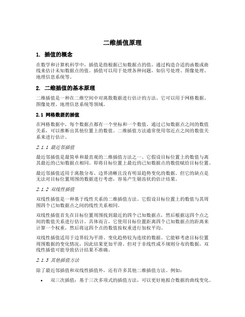
二维插值原理1. 插值的概念在数学和计算机科学中,插值是指根据已知数据点的值,通过构造合适的函数或曲线来估计未知数据点的值。
插值可以用于处理各种问题,如信号处理、图像处理、地理信息系统等。
2. 二维插值的基本原理二维插值是一种在二维空间中对离散数据进行估计的方法。
它可以用于网格数据、图像处理、地理信息系统等领域。
2.1 网格数据的插值在网格数据中,每个数据点都有一个坐标和一个数值。
通过已知数据点之间的数值关系,可以推断出其他位置上的数值。
二维插值方法通常使用邻近点之间的数值关系来进行估计。
2.1.1 最近邻插值最近邻插值是最简单和最直观的二维插值方法之一。
它假设目标位置上的数值与离其最近的已知数据点相同。
即将目标位置上最近的已知数据点的数值赋给目标位置。
最近邻插值适用于离散分布、边界清晰且没有明显趋势变化的数据。
但它的缺点是无法对目标位置周围的数据进行考虑,容易产生锯齿状的估计结果。
2.1.2 双线性插值双线性插值是一种基于线性关系的二维插值方法。
它假设目标位置上的数值与其周围四个已知数据点之间的线性关系相同。
双线性插值首先在目标位置周围找到最近的四个已知数据点,然后根据这四个点之间的数值关系进行估计。
具体而言,它使用目标位置距离四个已知数据点的距离来计算一个权重,然后将这四个点的数值按权重进行加权平均。
双线性插值适用于边界较为平滑、变化趋势较为连续的数据。
它能够考虑目标位置周围数据的变化情况,因此结果更加平滑。
但对于非线性或不规则分布的数据,双线性插值可能导致估计结果不准确。
2.1.3 其他插值方法除了最近邻插值和双线性插值外,还有许多其他二维插值方法。
例如:•双三次插值:基于三次多项式的插值方法,可以更好地拟合数据的曲线变化。
•样条插值:通过构造光滑的曲线来估计数据点之间的数值关系。
•克里金插值:基于空间自相关性的插值方法,可以考虑数据点之间的空间关系。
这些方法各有优缺点,适用于不同类型的数据和问题。
matlab中二维插值函数用法
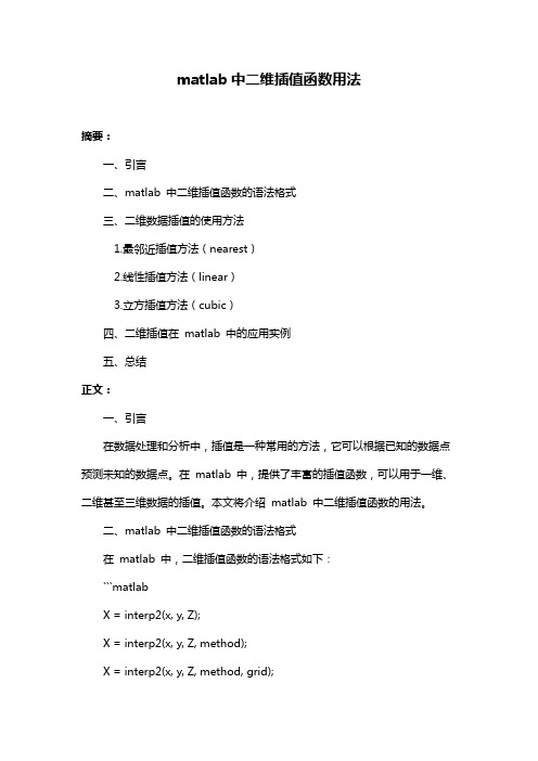
matlab中二维插值函数用法摘要:一、引言二、matlab 中二维插值函数的语法格式三、二维数据插值的使用方法1.最邻近插值方法(nearest)2.线性插值方法(linear)3.立方插值方法(cubic)四、二维插值在matlab 中的应用实例五、总结正文:一、引言在数据处理和分析中,插值是一种常用的方法,它可以根据已知的数据点预测未知的数据点。
在matlab 中,提供了丰富的插值函数,可以用于一维、二维甚至三维数据的插值。
本文将介绍matlab 中二维插值函数的用法。
二、matlab 中二维插值函数的语法格式在matlab 中,二维插值函数的语法格式如下:```matlabX = interp2(x, y, Z);X = interp2(x, y, Z, method);X = interp2(x, y, Z, method, grid);```其中,x 和y 是插值点的横纵坐标,Z 是插值点的高度(或者说是第三维),method 是插值方法,grid 是插值网格。
三、二维数据插值的使用方法1.最邻近插值方法(nearest)最邻近插值方法(nearest)是二维插值中最简单的插值方法,它将插值点落在离它最近的数据点上。
使用方法如下:```matlabX = interp2(x, y, Z, "nearest");```2.线性插值方法(linear)线性插值方法(linear)是二维插值中最常用的插值方法,它根据插值点的坐标和附近数据点的值进行线性插值。
使用方法如下:```matlabX = interp2(x, y, Z, "linear");```3.立方插值方法(cubic)立方插值方法(cubic)是二维插值中精度较高的插值方法,它根据插值点的坐标和附近数据点的值进行三次样条插值。
使用方法如下:```matlabX = interp2(x, y, Z, "cubic");```四、二维插值在matlab 中的应用实例下面我们通过一个实例来说明二维插值在matlab 中的用法。
VC++编写一维插值、二维插值代码

VC++智能读取TXT数据文件的代码工程师们在编写代码作各种工程计算的时候,很多时候会从外部TXT文件中读取数据。
读入的数据通常作为一个二维矩阵存储起来,以供各类封装函数调用。
读取数据的基本原则是,准确且完整的描述读取的数据内容,必须准确读取数值、准确识别二维数据的行列数。
数据的使用通常是对其按照行列进行二维插值,以下代码完成读取TXT文件数据后,对该二维矩阵进行二维差值。
首先,预定义一维整形动态数组用于存储TXT数据的行列数,预定义二维浮点型动态数组用于存储TXT数据的行列数,如下:#define I1vect vector< int >#define D1vect vector< double >#define D2vect vector< vector< double > >函数声明与定义:double interp1(D1vect x, D1vect y, double xt, char key)一维插值函数形参分别为:D1vect x,对应自变量向量;D1vect y,对应因变量向量;double xt,用于插值的点;char key,key=0代表内插值,key=1代表外插。
double interp2(D2vect data, I1vectlh, double xt, double yt, char key)一维插值函数形参分别为:D2vect data,二维浮点型数据矩阵;Ivect lh,二维整型数据矩阵,存放data矩阵的列数和行数,即lh(0) = 列数;lh(1) = 行数D1vect x;double xt,用于插值的点的横坐标;double yt,用于插值的点的纵坐标;char key,key=0代表内插值,key=1代表外插。
一维插值调用代码示例:D1vect x, y;Double xt,Int key = 0; // 或1yt = interp1(x, y, x, key);一维插值调用代码示例:D2vect data;I1vect lh;double xt, yt;Int key = 0; // 或1yt = interp2(data, lh, xt, yt, key); 完整代码见下一页。
图像的降采样与升采样(二维插值)

图像的降采样与升采样(⼆维插值)图像的降采样与升采样(⼆维插值)1、先说说这两个词的概念:降采样,即是采样点数减少。
对于⼀幅N*M的图像来说,如果降采样系数为k,则即是在原图中每⾏每列每隔k个点取⼀个点组成⼀幅图像。
降采样很容易实现.升采样,也即插值。
对于图像来说即是⼆维插值。
如果升采样系数为k,即在原图n与n+1两点之间插⼊k-1个点,使其构成k分。
⼆维插值即在每⾏插完之后对于每列也进⾏插值。
插值的⽅法分为很多种,⼀般主要从时域和频域两个⾓度考虑。
对于时域插值,最为简单的是线性插值。
除此之外,Hermite插值,样条插值等等均可以从有关数值分析书中找到公式,直接代⼊运算即可。
对于频域,根据傅⾥叶变换性质可知,在频域补零等价于时域插值。
所以,可以通过在频域补零的多少实现插值运算。
2、实现其实在matlab中⾃带升采样函数(upsample)和降采样函数(downsample),读者可以查找matlab的帮助⽂件详细了解这两个函数。
在这⾥,我重新写如下:%========================================================% Name: usample.m% 功能:升采样% 输⼊:采样图⽚ I, 升采样系数N% 输出:采样后的图⽚Idown% author:gengjiwen date:2015/5/10%========================================================function Iup = usample(I,N)[row,col] = size(I);upcol = col*N;upcolnum = upcol - col;uprow = row*N;uprownum = uprow -row;If = fft(fft(I).').'; %fft2变换Ifrow = [If(:,1:col/2) zeros(row,upcolnum) If(:,col/2 +1:col)]; %⽔平⽅向中间插零%补零之后,Ifrow为row*upcolIfcol = [Ifrow(1:row/2,:);zeros(uprownum,upcol);Ifrow(row/2 +1:row,:)]; %垂直⽅向补零Iup = ifft2(Ifcol);end%========================================================% Name: dsample.m% 功能:降采样% 输⼊:采样图⽚ I, 降采样系数N% 输出:采样后的图⽚Idown% author:gengjiwen date:2015/5/10%========================================================function Idown = dsample(I,N)[row,col] = size(I);drow = round(row/N);dcol = round(col/N);Idown = zeros(drow,dcol);p =1;q =1;for i = 1:N:rowfor j = 1:N:colIdown(p,q) = I(i,j);q = q+1;endq =1;p = p+1;endend% ===========================================% 测试升采样和降采样的程序% author:gengjiwen , date:2015/05/10% 备注:测试完毕!%============================================clear;close all;I = imread('test1.jpg');I = rgb2gray(I);figure(1);imagesc(I);title('原图像');% 图像降采样figure;for ii = 2:2:8Idown = dsample(I,ii);subplot(2,2,ii/2);imagesc(Idown);str = ['downsample at N = ' num2str(ii)]; title(str);end% 图像升采样figure;for ii = 2:2:8Iup =usample(I,ii);subplot(2,2,ii/2);imagesc(abs(Iup));str = ['upsample at N = ' num2str(ii)]; title(str);end测试结果如下:3、结果分析降采样没什么可说的,其实在matlab中可以很⽅便的⽤冒号运算符实现,具体可以查看下matlab⾃带函数downsample的实现。
Excel表格中二维数值插值的操作方法
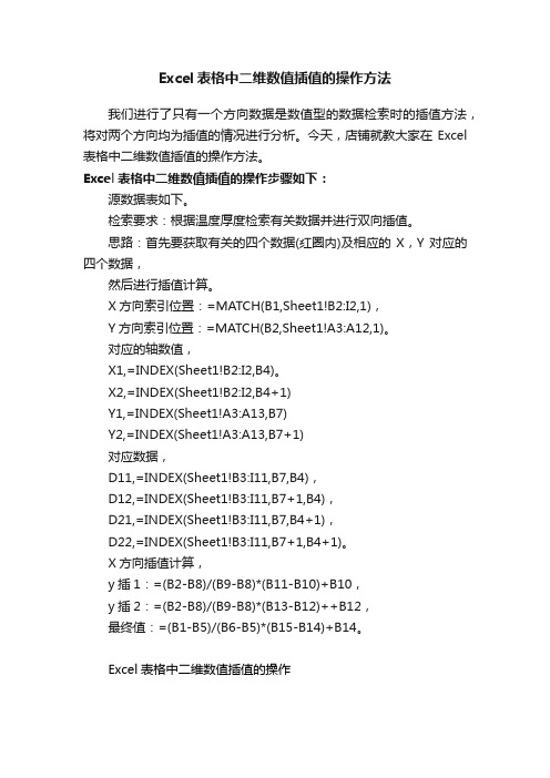
Excel表格中二维数值插值的操作方法
我们进行了只有一个方向数据是数值型的数据检索时的插值方法,将对两个方向均为插值的情况进行分析。
今天,店铺就教大家在Excel 表格中二维数值插值的操作方法。
Excel表格中二维数值插值的操作步骤如下:
源数据表如下。
检索要求:根据温度厚度检索有关数据并进行双向插值。
思路:首先要获取有关的四个数据(红圈内)及相应的X,Y对应的四个数据,
然后进行插值计算。
X方向索引位置:=MATCH(B1,Sheet1!B2:I2,1),
Y方向索引位置:=MATCH(B2,Sheet1!A3:A12,1)。
对应的轴数值,
X1,=INDEX(Sheet1!B2:I2,B4)。
X2,=INDEX(Sheet1!B2:I2,B4+1)
Y1,=INDEX(Sheet1!A3:A13,B7)
Y2,=INDEX(Sheet1!A3:A13,B7+1)
对应数据,
D11,=INDEX(Sheet1!B3:I11,B7,B4),
D12,=INDEX(Sheet1!B3:I11,B7+1,B4),
D21,=INDEX(Sheet1!B3:I11,B7,B4+1),
D22,=INDEX(Sheet1!B3:I11,B7+1,B4+1)。
X方向插值计算,
y插1:=(B2-B8)/(B9-B8)*(B11-B10)+B10,
y插2:=(B2-B8)/(B9-B8)*(B13-B12)++B12,
最终值:=(B1-B5)/(B6-B5)*(B15-B14)+B14。
Excel表格中二维数值插值的操作。
二维插值 原理

二维插值原理
二维插值是一种基于已知数据点的二维曲线或曲面估计方法。
它广泛应用于图像处理、地理信息系统、物理模拟等领域。
在二维插值中,我们假设已知的数据点位于一个二维平面上,每个数据点都有一个对应的数值。
我们的目标是通过这些已知数据点,来推断出未知位置上的数值。
常见的二维插值方法包括线性插值、拉格朗日插值和样条插值等。
线性插值是最简单的二维插值方法之一。
它假设在两个相邻数据点之间,数值的变化是线性的。
我们可以通过这两个相邻数据点之间的线段来估计未知位置上的数值。
拉格朗日插值则使用一个多项式来拟合已知数据点。
该多项式会经过所有已知数据点,并通过它们来估计未知位置上的数值。
它的优点是能够完全通过已知数据点来插值,但在高维情况下容易产生过拟合问题。
样条插值是一种基于局部插值的方法。
它通过在每个局部区域上拟合一个低阶多项式来实现插值。
这些局部多项式在相邻区域处满足平滑和连续性条件,从而得到整体平滑的插值结果。
除了上述方法外,还有其他一些二维插值方法,如反距离加权插值和克里金插值等。
总的来说,二维插值通过已知数据点之间的关系来估计未知位置上的数值。
不同的插值方法在计算复杂度、精度和平滑性等方面存在差异,根据具体应用场景的需求,选择合适的插值方法是非常重要的。
二维样条插值函数和二维牛顿插值

二维样条插值函数和二维牛顿插值二维样条插值函数和二维牛顿插值是在二维平面上进行插值的两种常见方法。
它们在科学计算、图像处理、地理信息系统等领域都有广泛的应用。
本文将对二维样条插值函数和二维牛顿插值进行详细介绍,并对它们的使用方法和特点进行比较。
首先,我们先来了解二维样条插值函数。
样条插值是一种光滑插值方法,它通过将插值函数拆分成多个小段,每个小段被称为样条。
二维样条插值函数是在二维平面上进行插值时使用的方法。
它的主要思想是将数据点之间的曲线进行拟合,得到一个平滑的曲线。
二维样条插值函数的插值曲线不仅能通过给定的数据点,还能将曲线的一阶和二阶导数保持连续。
这保证了插值曲线的光滑性和拟合性能。
在二维样条插值函数中,常用的有三次样条插值和二次样条插值。
三次样条插值利用三次多项式求解,保证了曲线的光滑性和连续性。
而二次样条插值只利用二次多项式,比三次样条插值的计算量要小,但相应地也降低了插值曲线的平滑性。
使用哪种样条插值函数要根据具体的应用场景和需求来选择。
接下来,我们来介绍二维牛顿插值。
二维牛顿插值是利用多项式进行插值的一种方法。
它通过构造一个多项式函数来拟合给定的数据点。
多项式的次数取决于数据点的个数。
二维牛顿插值的关键在于寻找插值节点和系数。
在二维牛顿插值中,插值节点的选取非常重要。
合理选择插值节点可以提高插值函数的拟合性能。
常见的选择方法有均匀节点选择和非均匀节点选择。
均匀节点选择是将二维平面均匀地划分成若干个小区域,然后在每个小区域内选择一个节点作为插值节点。
非均匀节点选择则根据数据点的密集程度来灵活选择节点,从而提高插值函数的拟合精度。
二维牛顿插值可以通过Newton的插值公式推导得到插值函数。
利用插值节点和数据点的差商来表示多项式的系数,从而得到插值函数。
同时,牛顿插值函数的计算速度相对较快,不需要拟合样条的复杂过程。
综上所述,二维样条插值函数和二维牛顿插值在二维平面上进行插值都有各自的特点和应用场景。
matlab interp2 用法
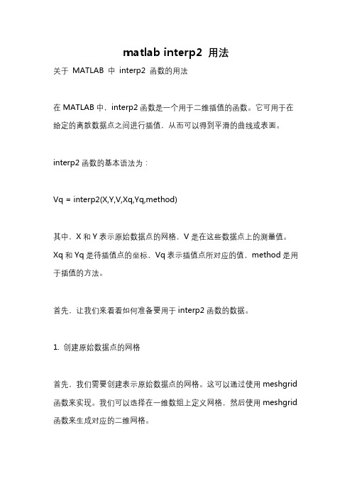
matlab interp2 用法关于MATLAB 中interp2 函数的用法在MATLAB中,interp2函数是一个用于二维插值的函数。
它可用于在给定的离散数据点之间进行插值,从而可以得到平滑的曲线或表面。
interp2函数的基本语法为:Vq = interp2(X,Y,V,Xq,Yq,method)其中,X和Y表示原始数据点的网格,V是在这些数据点上的测量值。
Xq和Yq是待插值点的坐标,Vq表示插值点所对应的值,method是用于插值的方法。
首先,让我们来看看如何准备要用于interp2函数的数据。
1. 创建原始数据点的网格首先,我们需要创建表示原始数据点的网格。
这可以通过使用meshgrid 函数来实现。
我们可以选择在一维数组上定义网格,然后使用meshgrid 函数来生成对应的二维网格。
例如,如果我们想要在x轴和y轴上分别有10个数据点,我们可以使用以下代码来创建网格:x = linspace(0,10,10);y = linspace(0,5,10);[X,Y] = meshgrid(x,y);这将创建一个10x10的网格,X和Y分别代表x和y坐标。
2. 创建原始数据点的测量值接下来,我们需要为每个数据点生成对应的测量值。
这些测量值可以是任意的,例如温度、压力、海拔等。
让我们用一个简单的函数来生成测量值,例如:V = sin(X).*cos(Y);这将为每个数据点生成一个sin(x)和cos(y)的乘积。
3. 进行插值接下来,我们可以使用interp2函数进行插值。
我们需要提供原始数据点的网格X和Y,以及每个数据点的测量值V。
我们还需要指定待插值点的坐标Xq和Yq,以及插值方法。
让我们使用与原始数据点相同的网格进行插值,并使用线性插值方法。
我们可以使用以下代码来实现:[Xq,Yq] = meshgrid(x,y);Vq = interp2(X,Y,V,Xq,Yq,'linear');注意,在这个例子中,我们使用的待插值点的坐标与原始数据点的网格相同。
二维数组使用拉格朗日插值算法

二维数组使用拉格朗日插值算法拉格朗日插值算法是一种用于二维数组的插值方法。
它通过对已知数据点的函数值进行逼近,可以在缺失数据的位置上给出一个合理的函数值。
这种方法是一种非常常用的数值分析算法,它可以广泛应用于工程、科学和其他领域。
下面我们将详细介绍二维数组使用拉格朗日插值算法的原理和步骤。
1. 基本原理拉格朗日插值算法的基本原理是通过已知数据点的函数值,对未知的函数值进行逼近。
具体来说,对于一组给定的插值点:(x0, y0), (x1, y1), (x2, y2), ..., (xn, yn)我们要在这些点的函数值上进行插值,在某个未知点(x, y)处给出一个函数值f(x, y)。
这个问题的解决方法就是求出一个多项式P(x, y),满足在插值点处P(x0, y0) = y0,P(x1, y1) = y1,..., P(xn, yn) = yn,并且f(x, y) = P(x, y)。
拉格朗日插值算法的多项式表达式如下:P(x, y) = Σ yiLi(x, y)其中Li(x, y)表示拉格朗日基函数,它的表达式为:Li(x, y) = Π(j ≠ i) (x - xj) / (xi - xj) * Π(k ≠ i) (y - yk) / (yi - yk)2. 插值方法具体来说,二维数组的拉格朗日插值算法分为下面四个步骤:(1) 选择一组插值点,构造出拉格朗日插值多项式。
(2) 在未知点(x, y)处代入多项式,求出函数值。
(3) 去掉一些离未知点较远的数据点,加入离未知点较近的数据点,重新构造出拉格朗日插值多项式。
(4) 重复执行第二步和第三步,直到满足一定的误差要求。
3. 算法实现(1) 定义一个数组data[N][N],存储网格的值,其中N为网格大小。
(2) 定义插值点的坐标(xi, yi),插值点的函数值fi。
可以选择一个较小的插值点集,并且随着插值迭代的进行,插值点的数量会不断增加。
(4) 定义一个函数Lagrange(data, xi, yi),求出在(x, y)处的函数值。
- 1、下载文档前请自行甄别文档内容的完整性,平台不提供额外的编辑、内容补充、找答案等附加服务。
- 2、"仅部分预览"的文档,不可在线预览部分如存在完整性等问题,可反馈申请退款(可完整预览的文档不适用该条件!)。
- 3、如文档侵犯您的权益,请联系客服反馈,我们会尽快为您处理(人工客服工作时间:9:00-18:30)。
上一页
下一页
x
主 页
引例2:船在该海域会搁浅吗?
在某海域测得一些点(x,y)处的水深z由下表给 出,船的吃水深度为5英尺,在矩形区域(75,200) *(-50,150)里的哪些地方船要避免进入。
x y z x y z 129 140 103.5 88 185.5 195 7.5 141.5 23 147 22.5 137.5 4 8 6 8 6 8 157.5 -6.5 9 107.5 -81 9 105 85.5 8
y y3 y2
(x*, y*)
y1
x1
x2
上一页
x3
下一页 主 页
x4
x5 x
二维插值的提法
第二种(散乱节点) 已知n个节点
其中
互不相同,
求任一插值点 处的插值
上一页 下一页 主 页
二维插值方法的基本思路
构造一个二元函数 通过全部已知节点,即
Y
3200 3000 2800 2600 1500 2000 X 2500
上一页 下一页 主 页
上一页
下一页
主 页
返回 上一页 下一页 主 页
范例2:船在该海域会搁浅吗?
在某海域测得一些点(x,y)处的水深z由下表给出, 船的吃水深度为5英尺,在矩形区域(75,200)* (-50,150)里的哪些地方船要避免进入。
范例1:绘制山区地貌图
分别用最近邻点插值、线性插 值和三次插值加密数据点,并分别 作出这三组数据点的网格图。
注意观察双线性插值方法和双三 次插值方法的插值效果的差异。
上一页 下一页 主 页
上一页
下一页
主 页
上一页
下一页
主 页
上一页
下一页
主 页
4500 4000 3500 3000 2500 2000 1500 1000 500 0
77 81 162 162 117.5 3 56.5 -66.5 84 -33.5 8 8 9 4 9
上一页
下一页
主 页
引例2:船在该海域会搁浅吗?
y
x
返回 上一页 下一页 主 页
插值的基本原理
二 维 插 值 的 提 法
第一种(网格节点)
注意:(x, y)当然应该是在插值节点所形成的矩形区 域内。显然,分片线性插值函数是连续的;
返回 上一页 下一页 主 页
3.双线性插值
y
(x1 y2) ,
(x2, y2)
(x1, y1) (x2, y1)
x
双线性插值是一片一片的空间二次曲面构成。 插值函数的形式如下: f ( x, y) (ax b)(cy d)
上一页
下一页
主 页
返回 上一页 下一页 主 页
用MATLAB作散点数据的插值计算
z=griddata(x0,y0,z0,x,y,’method’)
被插值点 的函数值
插值节点
被插值点
注意:x0,y0,z0均为向量,长度相等。
Method可取 ‘nearest’,’linear’,’cubic’,’v4’; ‘linear’是缺省值。
4500 4000 3500 3000 2500 2000 1500 1000 500 0
0
2000
4000
0
2000
4000
上一页
下一页
主 页
4200 4000 3800 3600 3400
4200 4000 3800 3600 3400
Y
3200 3000 2800 2600 1500 2000 X 2500
上一页 下一页 主 页
范例1:绘制山区地貌图
要在某山区方圆大约27平方公里范围内 修建一条公路,从山脚出发经过一个居民区, 再到达一个矿区。横向纵向分别每隔400米测 量一次,得到一些地点的高程:(平面区域 0<=x<=5600,0<=y<=4800),首先需作出该山 区的地貌图和等高线图。
上一页 下一页 主 页
xlabel('Width of Plate'), ylabel('Depth of Plate') zlabel('Degrees Celsius'), axis('ij'),grid, pause; zlin=interp2(width,depth,temps,wi,di,… 'cubic'); figure(3); mesh(wi,di,zlin) xlabel('Width of Plate'), ylabel('Depth of Plate') zlabel('Degrees Celsius'), axis('ij'),grid
或
再用
计算插值,即
返回 上一页 下一页 主 页
二维插值方法
网格节点插值法: 最邻近插值; 分片线性插值; 双线性插值; 双三次插值。 散点数据插值法:
修正Shephard法
上一页 下一页 主 页
返回
1.最邻近插值
y (x1, y2) (x2, y2) x
(x1, y1) (x2, y1)
求出测量范 围内的细网 格的节点的 x,y坐标数组
pf=griddata(x,y,z,px,py,’cubic’); figure(2),meshz(px,py,pf), rotate3d,pause
figure(3),surf(px,py,pf),
rotate3d,pause Contour(px,py,pf,
返回 上一页 下一页 主 页
用MATLAB作插值计算
网格节点的插值计算;
散点数据的插值计算;
用MATLAB作插值计算小结
返回 上一页 下一页 主 页
网格节点数据的插值
例:测得平板表面3*5网格点处的温度 分别为: x
82 79 84 81 63 84 80 61 82 82 65 85 84 81 86
数学实验之四
——(2)二维插值
实验目的
[1] 了解二维插值的基本原理,了解三 种网格节点数据的插值方法的基本思想; [2] 掌握用MATLAB计算二维插值的方法, 并对结果作初步分析; [3] 通过实例学习如何用插值方法解决 实际问题。
上一页
下一页
主 页
二维插值主要内容
引例1,引例2 二维插值的基本原理 二维插值方法
数值: f (xi, yj)=f1, f (xi+1, yj)=f2,
f (xi+1, yj+1)=f3,
第一片(下三角形区域):
f (xi, yj+1)=f4
插值函数为: f ( x, y) f1 (f 2 f1 )( x x i ) (f 3 f 2 )( y y j )
x y z x y z
129 140 103.5 88 185.5 195 105 7.5 141.5 23 147 22.5 137.5 85.5 4 8 6 8 6 8 8 157.5 107.5 77 81 162 162 117.5 -6.5 -81 3 56.5 -66.5 84 -33.5 9 9 8 8 9 4 9
用插值方法 求出网格节 点处的z坐 标矩阵, 并 作出三维图
figure(4),contour(px,py,pf,[-5 -5]); grid,pause
[i1,j1]=find(pf<-5);
for k=1:length(i1) pf(i1(k),j1(k))=-5; end figure(5) 图2到4: 利用网格 节点的x,y坐标向量 px,py及其对应的z 坐标矩阵pf,作出网 格线图和填充曲面图, 水深5英尺处海底曲 面的等高线
上一页 下一页 主 页
1.作出测量点的分布图
clear;
x=[129 140 103.5 88 185.5 195 105.5 157.5 107.5 77 81 162 162 117.5]; y=[7.5 141.5 23 147 22.5 137.5 85.5… -6.5 -81 3 56.5 -66.5 84 -33.5]; z=[-4 -8 -6 -8 -6 -8 -8 -9 -9 -8 -8 …
-9 -4 -9];
plot(x,y,'+');
pause
上一页 下一页 主 页
150
100
50
0
-50
-100 60
80
100
120
140
160
180
200
上一页
下一页
主 页
nx=100;
px=linspace(75,200,nx); ny=200;
py=linspace(-50,150,ny);
已知 mn个节点 (xi, xj, zij) ( i=1, 2, …,m; j=1, 2, …, n )
其中xi, yj互不相同,不妨设
a=x1<x2<…<xm=b c=y1<y2<…<yn=d
求任一插值点(x*, y*) ( ≠(xi, yj) )处的插值Z*
上一页 下一页 主 页
二维插值的提法
注意:最邻近插值一般不连续。具有连续性的最简 单的插值是分片线性插值。
返回 上一页 下一页 主 页
2.分片线性插值
y
(xi, yj+1) (xi+1, yj+1) (xi, yj) (xi+1, yj)