DEM-tutorial
英语单词

Indispensable[in+dis+pens+able]不不花钱被...的不得不被花钱买回来的Formal informalArms eg: arm to teethDisarmRespectful [ful= be full of ]respectableNegligent [neglig(neglect)+ent]会忽略掉其它事物的 = a. 疏忽的,Negligible [neglig(neglect+ible可被...的)] 可以被忽略掉的 - [neglect][neg=negative][lect=collect]Pens\pend=”花钱”1.Expensive[ex出去+pens+ive...的] = 贵的___ 出去了的 = 贵的2.Dispensable[indispensable的反义]a. 非必要的,可有可无的pensate[com相互+pens花钱,支付+ate...动作]1相互向对方支付费用 v. 赔偿,补偿,、Compensation [ion] n.赔偿,补偿,赔款Ion, ation, ition 加于动词后构成名词,不改变词义,常被理解为“原动作的过程或结果”Compose [com+pose(position)]摆放在一起Composition n. 作品Procedure - program4.Pension 【pens+ion】只花不赚的钱 -n. 养老金,退休金,抚恤金Pensioner [er] n. 退休人员 Retiree [ee]TireRetire [re回去+tire累]累了回家 - v. 退休Resign [re回去+sign签名]签名的回家- v. 辞职Retiree5.Expense [ex+pense]n. 花费,花销,代价(个人,家庭)Eg. At the expense ofExpenditureExpense v.s incomeDink: double incomes no kids2expenditure[ex出去+pend花钱+iture...物]n. 开支,开销Expenditure v.s revenue (总)收放,税收Eg. Military expenditure 军费开支Privilege [priv+i+lege]法律中给予某人的权力 - n. 特权Priv词根“私人,个人”1.Private [priv私人+ate...的] a. 私人的2.Privacy [acy抽象名词]私人的信息 = n. 隐私3.Deprive [de不+prive私人]使某物不再属于某人 - v. 剥夺,奔走Deprivation n.Rendezvous typhoonEg. Deprive sb of sthdeprive sb of his or her life-long political rightsLege词根“法律”1.Legal [leg+al...的] a. 合法的Eg. Entitle to some privilegesillegal [il(in)+legal]Inlegal way v.s in legal way3Legislate [leg(is)+late]【leg法律+is是+late后来】法律是在此动作后出现的 = v. 立法Dis gui se - guiseSan gui neNutrition把一种语言带入另一种语言Legislation n. Legislation hall Legislator [or] n.立法委员,立法者Legislature [ure] n. 立法机关Legislative [ive...的] a. 立法的Eg. Take legislative measuresLegitim ate[leg法律+it=?+im最...的+ate.=?...的]法律中最能接受的= a. 合理的Legitim acy [acy抽象名词]n. 合理性It=to\goexit [ex(out)+it(go)] n. 出口circuitous [circu(circle)+it走+ous...的]转圈走的= a. 环绕的Circulate4Im最...的(拉丁)Minimum [min小,少+im最..的+um..名]最小值Ultimate [ult完整+im最+ate.. 的]最完整的= a. 终极的,最终的UltSimultaneous[sim(same,similar)+ult完全+aneous...的] (时间)上完全相同的-a.同步的,同时进行的Eg. Simultaneous interpreterSyn chron ic = synchronize [syn\sym-same] Allege [al(ad强调)+lege法律]执意用法律解决问题=v. 控诉,指控,宣传Allegation n. 控诉,指控,宣传Jur\just\jud词根”法律”1.Judge n.Judgementjudgment v.Verdict[ver(very)+dict(predict先说-预言)]5Ver”真实,正确”a.VeryEg. You are the very person I am looking for.b. Verdict 说正确(公道)的话=n.仲裁,裁决c. Veri fy [ver正确+ify使...怎样]使某事正确= v. 核实,证实Veri fication n.Try-trial2.Prejudice[pre在...前+jud(judge)+ice...名] 提前对人作出判断- n偏见Bias [bi(bicycle, bi lingu al)]把人作为两种看待= n. 偏见Unbiased a.Lingu\langu - languageA.Lingu istB.Linguist ics [ics]C.Monolingual [mon=Monday monk moon]3.Justjustice n. Justice 司法Adjust [ad+just]6必需得刚好才行= v. 调节,调较Maladjustment [mal: maltreat, mal ign-ben ign] Beneficial - benefitBon\ben-bonus Bon Anne anniversary调节得不好= 紊乱,失调Justify v. 证明...正确或正当,证实Eg. Justi fy ing an assumptionJusti fication4.Juror [jur法律+or..人]参与法律判决的人= n. 陪审员Jury [y...集合] n. 陪审团Jurist [ist] n. 法学家Juridical 【jur+i+dic说话+al...的】拿法律说事的= a. 司法的Jurisdiction [ion] n. 司法权Dayu_998@Monopoly[mono+pol(pol ice man)+y]一个人管理= n.独裁,垄断,独占Monopolize [ize...动作]v. 垄断,独占7Mon\mun词根 moon1.Immune [im不+mune一]不能合为一体的=a.排斥的,免疫的,不受...影响的Eg. Be immune to sth 不受...影响的,免于...Immunity [ity...性质] n. 免疫力Immunize [immune+ize使...怎样]使某人对疾病免疫= v. 接种疫苗Immunization [ation...名] n. 接种疫苗Vaccine 疫苗 [vac空-vac ation] 3.Tele communicat ion n. 远程通信,电信TelecomTele远程的a.Telephone [sym phon y]b.Telegraph [graph] 在远端写出字c.Telescope4.Monolingual [l i ngu-l a ngu-language]5.Monograph [graph-paragraph]只写一方面= 专题论文,专著6.Monotonous[mono+tone语气,声调+ous]8一个调的= a. 单调的,枯燥的munity[com一起+mun一+ity...状态]共同呆在一起的状态n. 群落,共同体,社区,...界...圈Com mun ismShepherd [she e p + herd ]School flock crowd herdScholar scholarshipFeet fetter [fet(feet)+ter] 双写尾辅音加er表“小东西”Sol词根“数字1”1.Solo [sol]2.Sole3.Solar system \ energy4.Solid [sol+id具...性质的]一个是一个的-能看出个数来的n. 固体 a. 坚固的Consolidate [con相互+solid坚固+ate..动作]使相互间关系更坚固 = v. 巩固,加强,合并ConsolidationConsolidate - strengthen9Str o ng - str e ngth - strength enStrengthening growth of economyFast growth of economy合并,收购Merge merger n.Emerge [e出来+merge淹没]在被淹没的状态中出来 = v. 出现,浮现EmergingEg. Emerging economiesSubmergeAcquire [ac强调+quire寻求][quest(question-unquestionable)\quire\quisit] 一定要寻求到...= v. 获得,习得,收购Study scienceLearn a lesson fromAcquire knowledgeAcquisition n.Acquisitive [ive...的] 每样东西都想获得的Greed [grade-gradual] greedyM&A merger and acquisition5.Console [con+sole]单身的人来到一起= v. 安慰,抚慰6.Solitary10[sol+it去+ary...的]去一个人呆着的= a. 独居的,喜欢独处的7.Desolate [de离开+sol一+ate..动作] 离开某人使其变为一个人= v. 使孤寂,使凄惨Desolation n.8.I so late [i+sol+ate]Solate = so lateIsolation n.隔离Insulate insulation insulator - conductor - semi conductorInsul岛Insular [insul+ar...名词指人 ....的]Peninsula 【pen-pan】peninsularSegregate [seg切,分+reg管理+ate...动作] Segregation n.Seg\sect词根“切,分”SectionSegment11Reg词根“管理”RegionRegulateUn(i)词根“数字1”1.Unique [un+ique(ic...的)]一个的-a. 独特的,独一无二的,唯一的2.Reunion[re再一次+un一+ion...名]再一次来到一起的结果- n. 重聚,团聚3.Unify [un一+ify使...怎样]使一体化= v. 统一 Unification 民。
基于等高线的delaunay缝合算法分析与实现

To sum up, the research showed that the method presented in the thesis combined the advantages of
the Incremental Insertion Algorithm and Divide-and-conquer Algorithm. The method is easy to understand and its time complexity is close to linear. In conclusion, it’s a really practical algorithm.
Firstly,the experimental data was obtained through DXF-file. The 3D data on the contour lines was read and homogenized. Then the block-number was selected or input by the dialog interface. And the blocked data was stored in txt files block by block. Secondly, Delaunay Triangulation Networks were built according to the blocks, and the flat triangles of every network were converted after that. Thirdly, by searching and accessing the suturing edges, the suturing points were clockwise stored and divided into four parts according to four directions like top, right, bottom and left. In addition, the up and down blocks were sutured in the horizontal direction, after which the left and right blocks were sutured in the vertical direction. Finally, by optimizing the sutured triangulation network with the Local Optimal Procedure (LOP) algorithm, and converting the flat triangles, the Delaunay Triangulation model was established at last.
DEM基础知识整理---精品管理资料
DEM基础知识DEM即地面数字高程Digital Terrain Model,是地形表面形态属性信息的数字表达,是带有空间位置特征和地形属性特征的数字描述.如地面温度、降雨、地球磁力、重力、土地利用、土壤类型等其他地面诸特征.数字地形模型中地形属性为高程时称为数字高程模型.高程是地理空间中的第三维坐标.数学表达为:z = f(x,y)DEM是DTM的一个子集,是DTM的基础数据,最核心部分,可以从中提取出各种地形信息,如高度、坡度、坡向、粗糙度,并进行通视分析,流域结构生成等应用分析.DTM(Digital Terrain Model),数字地面模型是利用一个任意坐标系中大量选择的已知x、y、z的坐标点对连续地面的一种模拟表示,或者说,DTM就是地形表面形态属性信息的数字表达,是带有空间位置特征和地形属性特征的数字描述.x、y表示该点的平面坐标,z值可以表示高程、坡度、温度等信息,当z表示高程时,就是数字高程模型,即DEM。
地形表面形态的属性信息一般包括高程、坡度、坡向等。
数字高程模型是地形曲面的数字化表达,就是说,DEM是在计算机存储介质上科学、真实地描述、表达和模拟地形曲面实体,因此它的建立实际上是一种地形数据的建模过程。
DEM的建立首先要对地形曲面进行抽象、总结和提炼,形成高度概括的地形曲面数据模型,然后在此数据模型基础上,将观测数据按照一定的结构组织在一起,形成对数据模型的表述,最后借助计算机实现数据管理和地形重建。
1.DEM质量评价标准保凸性:若逼近面与实际曲面的波动次数相等或接近,而且两者对应的脊线、谷线位置和走向基本一致,则保凸性好,反之保凸性差。
逼真性:逼近面F(x,y)和实际地形曲面f(x,y)对应点之间应满足关系式:MAX|f(x,y)—F(x,y)|≤σ,则认为逼近面达到逼真性要求。
光滑性:光滑性是指曲线上切线方向变化的连续性,或者说曲线上曲率的连续性。
曲线的平顺性指曲线上没有太多的拐点。
ASTER_gdem_version2
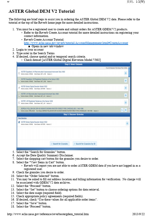
ASTER Global DEM V2 TutorialThe following are brief steps to assist you in ordering the ASTER Global DEM V2 data. Please refer to the tutorial at the top of the Reverb home page for more detailed instructions.1.You must be a registered user to create and submit orders for ASTER GDEM V2 products.◦Refer to the Reverb Create Account tutorial for more detailed instructions on registering yourcontact information.Reverb Create Account Tutorial:◦/reverb/tutorial/AccountManagement.html#CreateAccount ■Opens in new tab/window2.Login to your accountType aster in the Search Terms3.4.If desired, choose spatial and/or temporal search criteria.◦Check dataset [ASTER Global Digital Elevation Model V002]5.Select the “Search for Granules” button.6.Accept the Data Quality Summary Disclaimer.7.Select the shopping cart button for the granules you desire to order.Select the “View Items in Cart” button.8.◦Reverb will report you are not able to order ASTER GDEM data if you have not logged in as aregistered user.9.Check the granules you desire to order.10.Select the “Order Selected” button.11.You may be asked to fill out address location and billing information for verification. No charge will be associated with GDEM V2 data archives.12.Select the “Proceed” button.Select the “Set” button to choose ordering options for data retrieval.13.14.Select the data usage (required field).15.Check appropriate policy agreements (required fields).16.If desired, check “Use these values for all applicable order items”.17.Select the “Save” button.18.Select the “Proceed” button.Select the “Submit Order” button.19.20.Wait for email confirmation to retrieve data via FTP.21.Follow email directions to retrieve data.。
利用ENVI自带全球DEM数据计算区域平距高程
利用ENVI自带全球DEM数据计算区域平距高程ENVI是一种用于处理遥感数据的软件,它提供了自带的全球数字高程模型(DEM)数据集,可以用来计算区域的平均高程、距离和高度等信息。
在本文中,我将介绍如何使用ENVI来计算区域的平均距离和高度。
首先,我们需要加载ENVI软件,并导入全球DEM数据。
在ENVI中,可以通过选择“File”->“Open Data File”来导入全球DEM数据。
选择正确的文件路径,并确认已经正确地加载了DEM数据。
导入数据后,我们需要定义我们想要计算的区域。
可以使用ENVI的ROI工具来定义一个感兴趣的区域。
在ENVI中,选择“ROI”->“New ROI”来创建新的ROI。
然后,使用工具栏上的绘图工具来绘制一个多边形,定义我们感兴趣的区域。
绘制完成后,选择“ROI”->“Finish ROI”来完成ROI的定义。
此时,我们可以在ENVI的“ROI”窗口中看到我们创建的ROI。
接下来,我们可以使用ENVI的分析工具来计算区域的平均距离和高度。
在ENVI中,选择“Analyze”->“Terrain Analysis”->“Profile Surface”来计算剖面表面。
在“Profile Surface”对话框中,选择导入的全球DEM数据作为输入栅格,并选择我们定义的ROI作为输出区域。
点击“OK”按钮后,ENVI将计算区域的剖面表面。
完成后,我们可以在ENVI的“Image”窗口中看到生成的剖面图。
在该图像中,我们可以通过鼠标测量工具测量区域的平均距离和高度。
此外,除了计算区域的平均距离和高度,ENVI还提供了其他的地形分析工具,如计算地形坡度和方位等。
通过选择“Analyze”->“Terrain Anal ysis”菜单,我们可以使用这些工具来进一步分析区域的地貌特征。
总结起来,使用ENVI自带的全球DEM数据,我们可以很方便地计算区域的平均距离和高度。
dem实验报告
竭诚为您提供优质文档/双击可除dem实验报告篇一:Dem实验《gIs原理与应用》实验报告课程代码(0341552)姓名xxx学号xxx指导教师xxx目录实验一................................................. ..4第一部分实验目的 (4)1.1实验背景.................................................41.2通过本次实习需要掌握的内容 (4)1.3实习的具体内容 (4)第二部分实验流程 (5)2.1实验工具................................................. (5)2.11实习环境 (5)2.2实验内容 (5)第三部分实验总结 (9)3.1实验完成任务 (9)3.2实验小结 (1)5实验二................................................. .17第一部分实验目的 (17)1.1实验背景 (1)71.2通过本次实习需要掌握的内容 (19)1.3实习的具体内容 (19)第二部分实验流程 (19)2.1实验工具 (1)92.2实验内容 (1)9第三部分实验总结 (21)3.1实验完成任务 (21)3.2实验小结 (2)7实验三................................................. .28第一部分实验目的 (28)1.1实验背景 (2)8第二部分实验流程 (29)2.1实验工具 (2)92.2实验内容 (2)9第三部分实验总结 (31)3.1实验完成任务 (31)3.2实验小结 (3)4实验四................................................. .35第一部分实验目的 (35)1.1实验背景 (3)51.2通过本次实习需要掌握的内容 (35)1.3实习的具体内容 (35)第二部分实验流程 (35)2.1实验工具 (3)5(:dem实验报告)2.2实验内容 (3)6第三部分实验总结 (38)3.1实验完成任务 (38)3.2实验小结 (4)1实验五................................................. .42第一部分实验目的 (42)1.1实验背景 (4)21.2通过本次实习需要掌握的内容 (42)1.3实习的具体内容 (42)第二部分实验流程 (43)2.1实验工具 (4)32.2实验内容 (4)3第三部分实验总结 (44)3.1实验完成任务 (44)3.2实验小结 (4)7实验一—地形指标的提取第一部分实验目的1.1实验背景地形指标是最基本的自然地理要素,也是对人类的生产和生活影响最大的自然要素。
第4章DEM表面建模

• 虽然任何复杂曲面都可以由多项式在任 意精度上逼近,但在DEM内插中整体内 插并不常用。
缺点
(格网大小取决于DEM的应用目的),形成 覆盖整个区域的格网空间结构; • (2)利用分布在格网点周围的地形采样点内 插计算格网点的高程值; • (3)按一定的格式输出,形成该地区的格网 DEM。 • 关键环节:格网点高程的内插计算!
• 内插分类:
• (1)按数据分布
• 规则分布内插方法、不规则分布内插方法、等高线数据 内插方法
步长增大或缩小正方形边长。
逐点内插模型对数据量要求
内插函数模型 加权平均法 多层曲面叠加法 移动曲面拟合
采样点数量 4~10 4~10 >8
最小二乘拟合
>6
有限元内插
4~10
• 常用的邻域搜索区域有搜索圆和搜索正方形两种
• (1)搜索圆:
• 以当前内插点为圆心,按一定半径建立的圆形邻域, 该邻域的初始半径R可按下述经验公式确定:
•
4.3.3逐点内插法
• 逐点内插本质上是局部内插,但局部内插中的 分块范围一经确定,在整个内插过程中其大小、 形状和位置是不变的,凡是落在该块中的内插 点,都用该块的内插函数进行计算。
• 逐点内插法的邻域范围大小、形状、位置乃至 采样点个数随内插点的位置而变动,一套数据 只用来进行一个内插点的计算。
• (2)内插范围 • 整体内插方法、局部内插方法、逐点内插方法 • (3)内插曲面与采样点关系 • 纯二维内插、曲面拟合内插 • (4)内插函数性质 • 多项式内插:线性内插、双线性内插、高次多项式插值; • 样条内插;有限元内插;最小二乘配置内插 • (5)地形特征理解
德语词汇表-游戏篇1
德语词汇表-游戏篇11.die Konsole (-n) 游戏机Beispiel: Ich spiele gerne auf meiner Konsole. (我喜欢在我的游戏机上玩游戏。
)2.der Modding-Workshop (-s) MOD工作室Beispiel: In diesem Modding-Workshop kannst du lernen, wie du Mods erstellst. (在这个MOD工作室里,你可以学习如何创建MOD。
)3.das DLC (Downloadable Content) 下载内容Beispiel: Das neue DLC bringt viele neue Funktionen ins Spiel. (这个新的下载内容为游戏带来了很多新功能。
)4.die Spielmechanik (-en) 游戏机制Beispiel: Die Spielmechanik in diesem Spiel ist sehr interessant. (这个游戏的游戏机制非常有趣。
)5.der Spielverlauf (-verläufe) 游戏进程Beispiel: Der Spielverlauf in diesem Spiel ist sehr linear. (这个游戏的游戏进程非常线性。
)6.die Spielwelt (-en) 游戏世界Beispiel: Die Spielwelt in diesem Spiel ist sehr groß und detailliert. (这个游戏的游戏世界非常大而详细。
)7.die Spielphysik 游戏物理Beispiel: Die Spielphysik in diesem Spiel ist sehr realistisch. (这个游戏的游戏物理非常逼真。
)8.die Spielzeit (-en) 游戏时间Beispiel: Ich habe in diesem Spiel schon über 100 Stunden Spielzeit. (我已经在这个游戏中玩了100多个小时了。
02.Conveyor_Tutorial

Page 5 of 14
EDEM Tutorial: Conveyor
Step 3: Define the Geometry
Next we define the conveyor geometry used in the model.
Import the conveyor geometry
The conveyor geometry has been created in a CAD package ready for import into EDEM. 1. Click on the Geometry tab in the Tabs pane. 2. Click the Import button in the Sections section. 3. Navigate to the file conveyor_hopper.stp and import it. 4. When the Geometry Import Parameters dialog appears leave all the settings at the default values and click OK. 5. When prompted to, set the units of measurement to Millimeters. 6. The conveyor will appear in the Viewer. It is made up of five sections. Select and rename each section in the list. Name them guide_1, guide_2, lower_hopper, hopper and belt_top as appropriate. If necessary, change the material to steel for all sections.
常用遥感影像处理软件介绍及评价(下)
此外常用的还有:4 、ER MapperER Mapper 在142 个国家的用户使用着,全球有514 家销售商提供支持,是世界上最流行的桌面集成化图像处理软件。
使用广泛的图像使用强大的ER Mapper 智能,你可以轻松地将你的图像数据用一个无缝的镶嵌集成起来。
建立ER Mapper 聪明的数据算法提高图像质量,不需要临时的磁盘文件体验实时的处理。
采用压缩智能达到25 :1 的压缩比,使图像更易管理。
最好的是可以利用免费的ER Mapper 图像插件,与GIS 和Microsoft Office 用户共享你的图像和数据算法,插件支持Autodesk World, AutoCAD Map, ArcView 3.1, MapInfo, 以及OLE 程序,如Microsoft Word, Excel, Power Point. 用二维和三维展示你的工作使用ER Mapper 实时地对二维和三维的各种大小的图像进行漫游和缩放。
不需等待,不会混乱。
直接读取普通的图像格式,快速地开始工作。
在你的设计里将图像,向量图形,GIS 和表格组合成统一的视觉形象。
使用强大的全新的集成工具使用功能强大的衔接的集成工具,快速地将图像集成于你的应用流程中。
轻松操作正色摄影智能,图像显示和镶嵌智能,航片平衡智能和压缩智能,提供一个完全的集成方案。
提高你的工程成果需要突出显示火灾危险吗?要寻找新的城市发展吗?要完成一次环境影响的研究吗?要对重要地区更仔细的探测吗?使用功能强大的增效工具,如分类,FFT ,轮廓,从你的图像中提取出最多的信息。
生产成品质量的地图使用拖拽的地图产生工具建立成品质量的地图,并且采用自带的PostScript 兼容引擎输出生成极好的二维/ 三维效果的地图。
与GIS 和其它系统动态联接生成完整的表现,另外还有其它生产工具,如交互的轮廓生成,光栅图像和向量图形的转换。
使用免费的ER Mapper 评估版CD-ROM ,你会自己发现为什么ER Mapper 通过GIS 领域严格的比较后被评为图像处理产品的第一名5 、IDRISI Kilimanjaro 系统自从1987 年第一版IDRISI 软件诞生以来,克拉克实验室(Clark Lab )已经成功开发了14 个版本的IDRISI 软件。
DEM-复习整理

DEM-复习整理DEM 复习整理1、DEM概念(1)狭义概念: DEM是区域地表⾯海拔⾼程的数字化表达。
(2)⼴义概念: DEM是地理空间中地理对象表⾯海拔⾼度的数字化表达。
(3)数学意义: DEM是定义在⼆维空间上的连续函数H=f(x,y)2、数字⾼程模型的特点精度恒定性表达多样性更新实时性尺度综合性3、规则格⽹DEM和TIN的对⽐4、DEM数据模型从认知⾓度基于对象的模型、基于⽹络的模型、基于场的模型从表达⾓度⽮量数据模型镶嵌数据模型组合数据模型5、DEM数据结构(1)、规则格⽹DEM数据结构a、简单矩阵结构b、⾏程编码结构c、块状编码结构d、四叉树数据结构(2)、不规则三⾓⽹DEM数据结构TIN数据结构:⾯结构、点结构、点⾯结构、边结构、边⾯结构、简单结构(3)、格⽹与不规则三⾓⽹结构混合结构6、DEM数据源特征地形图、航空、遥感影像、野外测量、既有DEM数据可获得性(x,y,z)、DEM应⽤⽬的(分辨率、精度)、数据采集效率、数据量⼤⼩、技术熟练程度(1)数据源:地形图覆盖⾯⼴,可获取性强,是丰富、廉价的建⽴DEM的主要数据源。
特点:现势性(经济发达地区往往不满⾜现势性要求)、存储介质、精度:⽐例尺、等⾼线密度、成图⽅式有关(2)数据源:航空、遥感影像a、现势性好:获取速度快、更新速度快、更新⾯积⼤(⼤范围DEM数据的最有价值来源)b、缺点:受外界影响因素较⼤,对于精度要求⾼的DEM难以满⾜要求,⾼精度影像获取⽅法费⽤昂贵c、相对精度和绝对精度低的遥感影像: Landsat—MSS、TM传感器、SPOTd、⾼分辨率遥感图像:1⽶分辨率的IKONOS 0.61⽶QUICKBIRD(3)数据源:地⾯测量缺点:⼯作量⼤,周期长、更新⼗分困难,费⽤较⾼⽤途:公路铁路勘测设计、房屋建筑、矿⼭、⽔利等对⼯程精度要求较⾼的⼯程项⽬(4)数据源:既有DEM数据覆盖全国范围的1:100万、1:25万、1:5万数字⾼程模型7、数据采样⽅法对⽐(1)、地形图数据采集⽅法优点:a地形图易获取、作业设备简单、对操作⼈员技术要求较低,因⽽地形图是DEM获取最基本的⽅法。
DEM建立与应用

实习七、DEM建立与应用一、目的DEM是对地形地貌的一种离散的数字表达,是对地面特性进行空间描述的一种数字方法、途径,它的应用可遍及整个地学领域。
通过对本次实习的学习,我们应:1、加深对DEM建立过程的原理、方法的认识;2、熟练掌握ARCMAP中建立DEM、TIN的技术方法。
3、结合实际、掌握应用DEM解决地学空间分析问题的能力。
二、实验准备1、软件准备:ArcMap2、数据准备:文件feapt-clip1.dbf,feapt-clip1.shp,feapt-clip1.shx,文件terlk-clip1.dbf,terlk-clip1.shp,terlk-clip1.shx,文件夹cal2和info。
三、实验内容1、DEM及TIN的建立(1) 由采样点数据建立表面1)在视图目录表中添加并激活采样点层面feapt-clip1.shp。
2)从【Spatial Analyst】菜单中选择【Interpolate to Raster/Spline…】命令。
3)在Z Value Field列表中选择Elev(高程)字段,单击OK。
4)生成新的栅格主题Spline of feapt-clip1。
(2) 由点、线数据生成TIN转为GRID1)添加并激活点层面feapt-clip1。
2)点击【Spatial Analyst】菜单下的【Create /Modify TIN /Caeate Tin from features…】;3)在“Create New TIN”对话框中定义每个主题的数据使用方式;4)确定生成文件的名称及其路径,生成新的层面tin-point。
(见图4)5)点击【3D Analyst】菜单下的【Convert/TIN To Raster…】,确定生成文件的名称及其路径,生成新的Grid层面。
DEM的应用1)地形指标的提取坡度具体的方法步骤如下:1.添加Dem数据并激活它。
D:\arcgis\ArcTutor\Spatial\elevation)2.从【Surface Analysis】菜单中选择【Slope】命令。
ENVI(4.7)的教程

ENVI的教程:DEM模块的提取目录一、DEM模块的提取21、DEM在这个教程中使用22、DEM在工作中的应用2二、输入立体影像对3三、定义地面控制点4四、定义联接点51、编辑联接点72、计算极线几何和图片8五、指定参数101、投影DEM的参数指定输出102、DEM提取参数指定11六、检查结果121、显示加载DEM结果和表面三维视图的演示122、使用DEM编辑工具14七、使用立体3D测量工具16八、使用极3D光标工具17一、DEM模块的提取这次教程主要介绍了数字高程模型(DEM)提取模块与功能,使我们能够从立体图像提取海拔数据创建一个离散元法。
DEM是一种光栅的电网高程值所代表的表面。
DEM在许多场合都是有用的如映射,orthorectification,土地分类。
它经常被用来创建轮廓图和透视,地图和不同类型的土地利用规划的应用。
DEM提取模块使您能够从扫描或数字天线上照片,或从一个沿线阵式轨道卫星中提取海拔数据。
例如那些从低于平均值,CARTOSAT-1棱镜,FORMOSAT-2 abstracts 2002 vol . 72 no . KOMPSAT-2 IKONOS,GeoEye-1,OrbView-3, QuickBird,WorldView-1, SPOT satellites。
沿着轨迹获得立体影像, 同一个轨道卫星,它通常有多个传感器来从不同的角度看地球;立体影像就是取在多个轨道上的卫星的传感器所获得的地球上同一位置的影像。
DEM提取工艺需要一个立体声和一双图像包含理性的多项式系数(RPC)定位,无论是航空摄影或线阵传感器都可以被用来产生对RPCs联接点和计算立体图像联系,建立RPCs可以为用户指南提供指导细节。
DEM提取目前并不支持更换传感器模型(气)的精确定位。
DEM提取模块是组成的DEM提取的安装向导和三个DEM工具:编辑工具,立体对DEM数据的三维测量工具,以及极3D光标工具(注:DEM提取模块需要一个附加的许可,在你的安装的时候联系你的销售代表取得许可证。
英语词汇轻松学,大学和学院的名词.形容词.动词单词汇总english
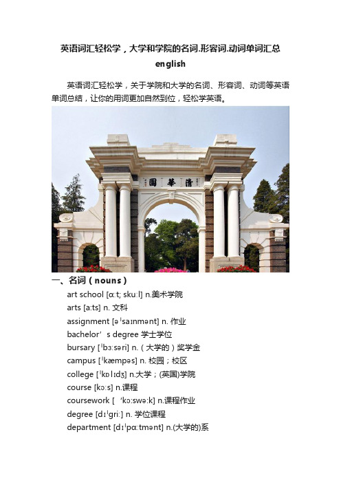
英语词汇轻松学,大学和学院的名词.形容词.动词单词汇总english英语词汇轻松学,关于学院和大学的名词、形容词、动词等英语单词总结,让你的用词更加自然到位,轻松学英语。
一、名词(nouns)art school [ɑːt; skuːl] n.美术学院arts [a:ts] n. 文科assignment [əˈsaɪnmənt] n. 作业bachelor’s degree 学士学位bursary [ˈbɜːsəri] n.(大学的)奖学金campus [ˈkæmpəs] n. 校园;校区college [ˈkɒlɪdʒ] n.大学;(英国)学院course [kɔːs] n.课程coursework [‘kɔ:swə:k] n.课程作业degree [dɪˈɡriː] n. 学位课程department [dɪˈpɑːtmənt] n.(大学的)系diploma [dɪˈpləʊmə] n.文凭课程;文凭distance learning 远程教育essay [ˈeseɪ] n.文章;论文exam [ɪɡˈzæm] n.考试examination [ɪɡˌzæmɪˈneɪʃn] n.考试faculty [ˈfæklti] n. (高等院校的)系;院fieldwork [ˈfiːldwɜːk] n.实地研究;野外考察finals [‘fainəlz] n.期末考试first [fɜːst] n.(英国大学学位)最高成绩;优等成绩graduate [ˈɡradʒʊeɪt] n.大学毕业生;学士学位获得者graduation [ˌɡrædʒuˈeɪʃn] n. 毕业典礼grant [ɡrɑːnt] n. 拨款halls of residence (大学)学生宿舍honours degree 荣誉学位invigilator [ɪnˈvɪdʒɪleɪtə(r)] n.监考人law school 法学院lecture [ˈlektʃə(r)] n.讲座major [ˈmeɪdʒə(r)] n.主修课程,专业master’s degree 硕士学位medical school 医学院natural sciences 自然科学PGCE [ˌpiː dʒiː siːˈiː] n.研究生教育证书PhD n.哲学博士学位;博士学历plagiarism [ˈpleɪdʒərɪzəm] n.抄袭,剽窃prospectus [prəˈspektəs] n.简章;简介reading list [ˈriːdɪŋ;lɪst] n. 阅读书目research [rɪ’sɜːtʃ] n. 调查,研究scholarship [ˈskɒləʃɪp] n.奖学金school [skuːl] n. 学院semester [sɪˈmestə(r)] n. 学期seminar [ˈsemɪnɑː(r)] n.研讨课social sciences [ˈsəʊʃl;’saɪəns] n.社会科学student [ˈstjuːdnt] n. 学生student accommodation 学生宿舍student loan 学生贷款student union 学生会;学生活动中心syllabus [ˈsɪləbəs] n.教学大纲technical college 技术学校term [tɜːm] n. 学期thesis [ˈθiːsɪs] n.论文tuition fees 学费tutor [ˈtjuːtə(r)] n.导师;指导教师tutorial [tjuːˈtɔːriəl] n.参加研讨课;大学导师的辅导课undergraduate [ˌʌndəˈɡrædʒuət] n.大学本科生university [ˌjuːnɪˈvɜːsəti] n.大学;高等学府viva [ˈviːvə] n.口试vocational course 职业课程二、动词(verbs)enroll [ɪn’rəʊl] v. 使加入;招生graduate [ˈɡradʒʊeɪt] v. 毕业invigilate [ɪnˈvɪdʒɪleɪt] v.监考register [ˈredʒɪstə(r)] v. 注册;登记study [ˈstʌdi] v. 学习;攻读work [wɜːk] v.工作三、形容词(adjectives)academic [ˌækəˈdemɪk] adj. 学术的full-time [,fʊl’taɪm] adj. 全日制的part-time [,pɑ:t’taɪm] adj. 部分时间的。
DEM复习重点

DEM复习重点1.数字高程模型是通过有限的地形高程数据实现对地形曲面的数字化模拟或者说是地形表面形态的数字化表示。
2.数字地面模型DTM是定义在二维区域上地形特征空间分布及关联信息的一个有限n维向量系列Xi,数字高程模型DEM是DTM的一个子集,它表示地形空间分布的一个有限三维向量。
3.DEM:狭义角度是区域地表面海波高度的数字化表达。
广义角度是地理空间中地理对象表面海波的数字化表达。
4.基于规则格网的DEM和基于TIN的DEM是目前数字高程模型的两种主要结构。
5.数字高程模型的主要研究内容:1)地形数据采样2)地形建模与内插3)数据组织与管理4)地形分析与地学应用5)DEM可视化6)不确定性分析与表达6.数字高程模型的分类体系:范围(局部DEM、地区、全局)。
连续性(不连续DEM、连续、光滑)。
结构)面(规则结构:正方形格网结构、正六边形格网结构、其他格网结构)、(不规则结构:不规则三角网、四边形)线(等高线结构、断面结构)点(散点结构)。
7.数字高程模型的特点:1)精度恒定性2)表达多样性3)更新时实行4)尺度综合性8.DGM:除高程外,地形表面形态还可通过坡度。
坡向、曲率等地貌因子进行描述。
所有地貌银子的数字模型的集合形成数字地面模型DGM9.DTM:各种地物要素的数字模型,连同DEM本身,形成测绘人员心目中新一代地形图,数字定型模型DTM10.DSM:一般的,将DEM/DGM/DTM以及上述信息所形成的数字模型称为数字表面模型11.DEM(--DGM(--DSM层层包含关系DEM是最基本的数据12.数字高程模型的应用范畴:1)地学分析应用2)非地形特征应用3)产业化和社会化服务13.DEM主要用在一下几个领域:1)区域、全区气候变化研究2)水资源、野生动植物分布3)地质水文模型建立4)地理信息系统5)地形地貌分析6)土地分类、土地利用、土地覆盖变化检测等第二章DEM数据组织与管理14:目前GIS中的空间数据模型从认知角度讲有三类,即基于对象的模型、基于网络的模型、基于场的模型:从表达上讲有矢量数据模型、栅格数据模型和组合数据模型。
DEM制作流程
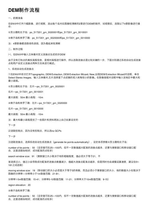
DEM制作流程⼀、前期准备在ENVI中打开六幅影像,进⾏观察,选出每个岛对应图像较清晰的2景进⾏DEM的制作,经观察后,选取以下4景影像进⾏操作:①贡⼠礁和北⼦岛:po_517201_grn_0020001和po_517201_grn_0010001②南⼦岛和奈罗丁礁:po_517201_grn_0020000和po_517201_grn_0010000注:4景影像都选取绿⾊波段,因为看起来较清晰⼆、制作过程㈠、在ENVI中输⼊⽴体像对定义连接点⽣成初步DEM由于没有已知点的真实⾼程信息,是相对⾼程进⾏操作,所以选取连接点是⽐较关键的⼀步,下⾯分别通过系统⾃动⽣成连接点和⽤户⾃定义连接点两种⽅法来进⾏阐述。
1、系统⾃动⽣成连接点⑴在ENVI中依次打开Topographic, DEM Extraction, DEM Extraction Wizard, New,出现DEM Extraction Wizard对话框,单击Select Stereo Images,输⼊⽴体像对,左⽚选择星下点成像的或⼊射⾓较⼩的影像。
在影像⾼程对话框中输⼊该地区中最⼤和最⼩⾼程。
①贡⼠礁和北⼦岛:左⽚—po_517201_grn_0020001右⽚—po_517201_grn_0010001最⼤⾼程:50m 最⼩⾼程:-10m②南⼦岛和奈罗丁礁:左⽚—po_517201_grn_0020000右⽚—po_517201_grn_0010000最⼤⾼程:50m 最⼩⾼程:-10m注:最⼤和最⼩⾼程是找了⼀些图⽚和资料再加上⾃⼰估算设定的下⼀步⑵选取控制点,因为没有控制点,所以选no GCPs下⼀步⑶选取连接点,选择系统⾃动⽣成连接点(generate tie points automatically),设定各项参数①贡⼠礁和北⼦岛:number of tie points :50 (设定值可在25—100内,但不⼀定数值越⼤配准的连接点越多,还要与搜索窗⼝和移动窗⼝配合,这⾥选取50较好,成功配准的点较多)search window size:91 (搜索窗⼝⼤⼩取决于地形粗糙程度,值必须⼤于等于21,不宜选择过⼩,值过⼩会导致成功配准的连接点数量减少,值越⼤连接点配准点越多,但是同时也会减慢运算速度,建议在51-181之间选取)moving window size:19 (移动窗⼝的⼤⼩必须是⼤于等于5的奇数,⽽且必须⼩于搜索窗⼝的⼤⼩,他的数值⼤⼩也取决于图像的分辨率—分辨率⼩于1m取值范围:21-81;分辨率1-5m取值范围:15-41;分辨率5-10取值范围:11-21;分辨率⼤于10m取值范围:9-15)region elevation:20②南⼦岛和奈罗丁礁:number of tie points :50 (设定值可在25—100内,但不⼀定数值越⼤配准的连接点越多,还要与搜索窗⼝和移动窗⼝配合,这⾥选取50较好,成功配准的点较多)search window size:91 (搜索窗⼝⼤⼩取决于地形粗糙程度,值必须⼤于等于21,不宜选择过⼩,值过⼩会导致成功配准的连接点数量减少,值越⼤连接点配准点越多,但是同时也会减慢运算速度,建议在51-181之间选取)moving window size:11region elevation:20下⼀步⑷连接点配准出现校准对话框,可以通过“likely error ranking”来查看各连接点的错误概率排序,点击检查每⼀个点来校准,可以通过系统⾃动预测“predict”或⼿动修正使“maximum Y parallax”的数值⼩于10,即可进⾏下⼀步操作,在本次操作中:贡⼠礁和北⼦岛:7.6573南⼦岛和奈罗丁礁:8.0234下⼀步⑸构建核共线影像影像,创建并保存左影像和右影像。
利用python和DEM数据实现坡度计算
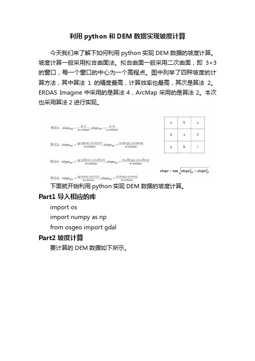
利用python和DEM数据实现坡度计算今天我们来了解下如何利用python实现DEM数据的坡度计算。
坡度计算一般采用拟合曲面法。
拟合曲面一般采用二次曲面,即3×3的窗口,每一个窗口的中心为一个高程点。
图中列举了四种坡度的计算方法,其中算法1的精度最高,计算效率也最高,其次是算法2。
ERDAS Imagine中采用的是算法4,ArcMap采用的是算法2。
本次也采用算法2进行实现。
下面就开始利用python实现DEM数据的坡度计算。
Part1导入相应的库import osimport numpy as npfrom osgeo import gdalPart2坡度计算要计算的DEM数据如下所示。
先读取DEM数据,并初始化输出。
dem_ds = gdal.Open(dem)cell_width = dem_ds.GetGeoTransform()[1]cell_height = dem_ds.GetGeoTransform()[5]band = dem_ds.GetRasterBand(1)in_data = band.ReadAsArray().astype(np.float)out_data = np.ones((band.YSize, band.XSize)) * -99 #初始化输出利用make_slices函数(详见附录)进行数据切片,make_slices返回的是一个长度为9的列表,每一个列表中的值分别对应3*3窗口中9个输入像素的对应集合。
然后计算坡度,注意此时计算出来的结果不包括原DEM数据中最外围的像素点,所以输出的时候out_data最外围的一圈仍是初始化的值。
slices = make_slices(in_data,(3,3))rise= ((slices[6] + (2 *slices[7]) + slices[8])- (slices[0]+(2*slice s[1])+slices[2]))/(8*cell_height)run = ((slices[2] + (2*slices[5])+slices[8])-(slices[0]+(2*slices[3])+slices[6]))/ (8*cell_width)dist = np.sqrt(np.square(rise)+np.square(run))out_data[1:-1,1:-1] = np.arctan(dist)*180 /np.pi利用make_raster函数(详见附录)输出坡度结果,保存为tif。
- 1、下载文档前请自行甄别文档内容的完整性,平台不提供额外的编辑、内容补充、找答案等附加服务。
- 2、"仅部分预览"的文档,不可在线预览部分如存在完整性等问题,可反馈申请退款(可完整预览的文档不适用该条件!)。
- 3、如文档侵犯您的权益,请联系客服反馈,我们会尽快为您处理(人工客服工作时间:9:00-18:30)。
Modeling bubbling fluidized bed using DDPM+DEMIntroductionThe DEM collision model extends the DPM model in Fluent to model dense particulate flows.pneumatic conveying systems, and the flow of slurries. The DEM models is especially useful •When dealing with a wide particle size distribution•When dealing with relatively coarse meshesThis document is a tutorial on the use of the DDPM model where collisions are modeled through DEM model.PrerequisitesThis tutorial will not cover the mechanics of using the Dense DPM or DEM models. It will focus on the application of these models. For more information refer the ANSYS FLUENT User's Guide and Theory Guide. This tutorial is written with the assumption that you have completed Tutorial 1 from the ANSYS FLUENT 14.0 Tutorial Guide, and that you are familiar with the ANSYS FLUENT navigation pane and menu structure. Some steps in the setup and solution procedure will not be shown explicitly.Problem DescriptionIn this tutorial we will model a bubbling fluidized bed and determine its behavior for a given superficial velocity. A rectangular bed of size 0.2m * 0.2m * 0.4m is initially charged with particles, and the superficial velocity of the gas is 0.5 m/s. The pressure drop across the bed is monitored. Schematic of the problem is shown in Figure.1.From the classic fluidization curve, if the superficial velocity of the inlet fluid is small, the bed is not fluidized and behaves like a packed bed. As the velocity of the fluid is increased, the bed begins to fluidize.One of the classical ways to understand the phenomena is the fluidization curve; here the pressure required to pump the fluid at the inlet is studied as a function of the superficial velocity. Under packed bed conditions, there is a linear increase in the pressure as the superficial velocity is increased. However, this increase begins to taper off as the condition of incipient fluidization is reached, and the pressure reaches a constant value (in a time averagedsense). This constant pressure at fluidization conditions is sufficient to maintain the buoyant weight of the bed. In other words<ܲ>௧ × ܣ௧= Buoyant weight of bedIn this tutorial we will perform simulations for a given superficial velocity where a bed is fluidized. It will be left upon the user to try with different superficial velocity to obtain the fluidization curve.Figure.1: Schematic of problem descriptionPreparationA.Copy the files bed.msh, 92Kparcels.inj and view-0.vw to the working folder.e FLUENT Launcher to start the 3D version of ANSYS FLUENT.Note: For more information about FLUENT Launcher see Section 1.1.2 Starting ANSYS FLUENTusing FLUENT Launcher in the ANSYS FLUENT 14.0 User's Guide.C.Enable DoublePrecision in the Options list.Note: The Display Options are enabled by default. Therefore, after you read in themesh, it will be displayed in the embedded graphics window.Setup and SolutionNote: All entries in setting up this case are in SI units, unless otherwise specified.Step 1: Mesha)Read the mesh file bed.msh.File Read Mesh...Step 2: Generala)Check the mesh.General CheckANSYS FLUENT will perform various checks on the mesh and will report the progress in the console. Ensure that the minimum volume reported is a positive number.b)Enable the transient solver by selecting Transient from the Time list.General TransientStep 3: Modelsa)Multiphase model.Models Multiphase Edit…I.Select Eulerian multiphase model.II.Enable Dense Discrete Phase Model.III.Retain other defaults and click OK.Figure.2: Multiphase Model Panelb)Discrete Phase Model.Models Discrete Phase Edit…I.Make sure that Update DPM Sources Every Flow Iteration.II.Enter 200 for Number of Continuous Phase Iterations per DPM Iteration.III.Make sure that Unsteady Particle Tracking is enabled.IV.Disable Track with Fluid Flow Time Step and enter 0.0002 for Particle Time Step Size (s).V.Enable DEM Collision under Physical Models tab.VI.Set Drag Law as Wen-Yu under Tracking Tab.VII.Set the following under Numerics tab.•Disable Accuracy Control.•Select implicit as Tracking Scheme.VIII.Click OK to close DPM panel.Figure.3: Discrete Phase Model Panelc)Define Injection.Define Injections… CreateI.Select file under Injection Type.II.Select phase-2 under Discrete Phase Domain.III.Enter 1e-8 for Stop Time (s).IV.Click File… button and select 92Kparcels.inj file from working folder.V.Click OK to close Set Injection Properties panel.VI.Click Close to close Injections panel.Figure.4: Set Injection Properties Paneld)Set DEM collision laws.Models Discrete Phase Edit… DEM Collisions…I.Select dem-anthracite and click Set… This will open DEM Collision Settingspanel.II.Select dem-anthracite – dem-aluminum from Collision Pairs.III.Retain spring-dashpot as Normal Contact Force and set friction-dshf for Tangential.IV.Change spring-dashpot: k as 100 and spring-dashpot: eta as 0.5.V.Select dem-anthracite – dem-anthracite from Collision Pairs.VI.Retain spring-dashpot as Normal Contact Force and set friction-dshf for Tangential.VII.Change spring-dashpot: k as 100 and retain other settings.VIII.Click OK to close the panel.IX.Click Close to close DEM Collisions panel.X.Click OK to close DPM panel.Figure.5: DEM Collision Settings PanelStep 4: Phasesa)Set phase-2.Phases Phase-2 Edit...I.Deselect Volume Fraction Approaching Continuous Flow Limit and click OK.Step 5: Operating ConditionsDefine Operating Conditions…a)Enable Gravity and set Z component as -9.81 m/s2.b)Specify Operating Density to be 1.225 kg/m3.Step 6: Boundary ConditionsBoundary Conditionsa)Set boundary conditions for inlet.I.Select inlet from zone list and click Edit… while phase is mixture. This will openVelocity Inlet panel for mixture phase.II.Go to DPM tab and select Discrete Phase BC Type to reflect and DEM Collision Partner as dem-aluminum.III.Click OK to close this panel.IV.Select phase-1 from Phase drop down list and click Edit….V.Enter 0.5 for Velocity Magnitude (m/s) and click OK to close the panel.b)Set boundary conditions for outlet.I.Select outlet from zone list and click Edit…while phase is mixture. This willopen Pressure Outlet panel for mixture phase.II.Go to DPM tab and select Discrete Phase BC Type to reflect and DEM Collision Partner as dem-aluminum.III.Click OK to close this panel.c)Retain default settings for wall.Step 7: Solution MethodsSolution Methodsa)Select Green-Gauss Node Based from Gradient.b)Select QUICK for Momentum and Volume Fraction Spatial Discretization.Step 8: Solution ControlsSolution Controlsa)Set Under-Relaxation Factors for variables as given below.I.Pressure: 0.9II.Momentum: 0.2III.Volume Fraction: 1IV.Discrete Phase Sources: 1Step 9: MonitorsMonitors Surface Monitors Create…a)Create monitor of Area-Weighted Average of Static Pressure on inlet surface.b)Enable Plot and Write.c)Set X Axis as Flow Time and Get Data Every 1 Time Step.d)Click OK to close the panel.Figure.6: Surface Monitor PanelStep 10: Solution InitializationSolution Initializationa)Initialize with default settings. Click Initialize.Step 11: Calculation ActivitiesCalculation Activities Execute Commands Create/Edit…We will define four commands in this step which will save images of particle tracks colored by particle velocity magnitude at specified interval. These images can be clubbed together to create animation.a)Set Defined Commands to 4.b)Set execute commands as shown in the Figure.7 below.c)Set settings for saving images as shown in Figure.8.File Save Picture…Figure.7: Execute Commands PanelFigure.8: Save Picture PanelStep 12: Run CalculationRun CalculationWe will perform this step in three stages. First we will perform calculation for single time step to inject all particles in the domain. We would then set post-processing parameters which would be used to save image files at specific intervals as entered in Step 11. In the second stage, wewould run the calculation for two seconds of flow time with Execute Commands enabled. In the last stage, case will be run for two more seconds without Execute Commands.a)Set Time Step Size (s) as 0.001.b)Set Number of Time Steps as 1.c)Set Reporting Interval as 5.d)Click Calculate.e)Read view-0 from file view-0.vw from working folder.Display Views… Read…f)Create iso-surface of y-coordinate=0. Name it as y=0.Surface Iso-Surface…g)Display contour of phase-2volume fraction on iso-surface y=0. Make sure Filledand Node Values are enabled.Graphics and Animations Contours Set Up…h)Set Light settings. Make sure that Light On and Headlight On are enabled. SelectLighting Method as Gouraud.Display Lights…i)Set particle track settings as shown in Figure.9.Graphics and Animations Particle Tracksj) Click on Attributes… button under Track Style and select Parcel Diameter as shown in Figure.10.k)Click on Filter by… button and select Y-Coordinate and set Filter-Min, Filter-Max as shown in Figure.11.l)Click Display.Figure.9: Particle Tracks PanelFigure.10: Particle Sphere Style Attributes PanelFigure.11: Particle Filter Attributes Panelm)Save the case file as fbed-first-t-step.cas.gz.n)Run calculation for 2000 time steps.o)Disable Execute Commands by setting Defined Commands to 0under Execute Commands panel.p)Run calculation for 2000 time steps.q)Save case and data as fbed-final.cas.gz and fbed-final.dat.gz.Step 13: Resultsa)Figure.12 shows contour plot of secondary phase volume fraction, contour plot ofDPM Concentration and Particle tracks from the final data file. Notice that resultsare close.b)Figure.13shows plot of pressure drop across the bed. Notice that mean value isclose to the pressure drop equivalent for buoyant weight of the bed which is 981 Pa.Figure.12: Results from final data file.A.Contour plot of secondary phase volume fractionB.Contour plot of DPM ConcentrationC.Particle Tracks colored by secondary phase volume fractionFigure.13: Monitor plot for pressure drop across the bed。