Parasolid Geometry Modeling
ADINA几何建模专题知识讲座

几何建模
ADINA Native-生成线(Line)-多义线POLYLINE-三次样条
• 三次B样条曲线 除端点外,曲线不经过控制点;
• 双弧线-Bi-Arc
经过控制点;
除端点外,两点之间有两段圆弧光 滑连接;
几何建模
• 贝塞线-Bazier 除端点外,曲线不经过控制点;
ADINA Native-生成线(Line)-多义线POLYLINE
[A]
几何建模
ADINA Native-生成线(Line)-多义线POLYLINE-折线
• Straight Line Segments 按照一定顺序连接点形成多义线,此多
义线为折线;
阐明:不限点旳数目; 双击绿色空格,进入图形选择状态,
2 点击创建点旳图标,在定义点旳列表中删除相应点旳 一行定义,点击OK或Apply即可。
几何建模
ADINA Native-生成线(Line)-线类型
菜单:Geometry > Lines > Define... 生成线:
环节: 1. 点击ADD; 2. 选择线旳类型(涉及直线,多义线等多种形式。); 3. 输入定义线旳点及其可能需要旳其他参数; 4. SAVE或OK生成线;
几何建模
2. P1, P2, P3
P1:终点 P2:起点 P3:辅助点定义圆弧位于旳平面
阐明: 弧心点P4自动生成, 除非打开了反复点检 验选项而且在形心点处 已经有点;
ADINA Native-生成线(Line)-弧线
几何建模
3. P1, Center, Angle, P3
P1:起点 Center:中心点 Angle:圆心角 P3:圆弧平面辅助点
ANSYS导入CAD二维模型的方法
ANSYS导入CAD二维模型的方法在ANSYS中,可以通过两种方法将CAD二维模型导入到软件中:直接导入和间接导入。
直接导入方法:1.打开ANSYS软件并创建新项目。
2. 点击“Geometry”选项卡下的“DesignModeler”进入建模环境。
3. 在设计模型器中,选择“File”选项,然后选择“Import”选择CAD文件。
4. 在弹出的文件浏览器中,浏览并选择要导入的CAD文件。
ANSYS支持多种CAD文件格式,例如IGES,STEP,Parasolid等。
5. 点击“Open”按钮导入CAD文件。
此时ANSYS会将CAD文件转换为ANSYS本地文件格式(.agdb或.gbx等)。
6. 在CAD文件转换完成后,可以选择将整个CAD文件导入ANSYS环境中,或选择导入文件的特定几何实体。
要导入整个CAD文件,请选择“Import Full Model”选项,要选择特定几何实体,请选择“Import Geometry”选项。
间接导入方法:1.将CAD文件导入到ANSYS支持的中间格式中,例如IGES,STEP等。
2.打开ANSYS软件并创建新项目。
3. 点击“Geometry”选项卡下的“DesignModeler”进入建模环境。
4. 在设计模型器中,选择“File”选项,然后选择“Import”选择中间格式文件。
5.在弹出的文件浏览器中,浏览并选择导入的中间格式文件。
6. 点击“Open”按钮导入中间格式文件。
7.此时,ANSYS将导入的文件转换为其本地文件格式,并在设计模型器中显示。
需要注意的是,CAD文件的复杂性和几何实体的数量可能会影响导入的时间和成功率。
在导入过程中,可能需要进行一些后处理操作来修复不完整或不正确的几何实体。
一些高级的CAD文件可能需要进行进一步的处理才能正确导入。
在处理过程中,根据具体情况可能需要进行不同的调整和优化。
(转自仿真科技论坛)几乎所有的有限元分析的软件介绍——让你对CAE软件更了解
-------------------------------------------------------------------------------1649 AEGis.acslXtreme.v1.3.2 ACSLXTREME 英文 1.3.2 有限元分析 1CD 无 简单介绍:强大的连续动态系统建模工具,使用非常方便。acslXtreme复杂的下一代 连续动
求,AN
SYS Multiphysics 8.0推出了多物理场求解器,提供了一个易于应用的多物理场求解解决方案,实现对许 多新 兴市场和领域中耦合场问题的求解,而这在以前一直都是悬而未决的技术难点。新的 多物理
场求解器是一个通用的、全自动的序贯耦合多场求解器,适用于ANSYS Multiphysics中所有场分析能力之间的耦合计算,它也是在ANSYS以前成功推出的流 体-结构 耦合(FSI)求解器基础上的又一次革命性创举
-------------------------------------------------------------------------------974 Ansys AI Nastran 1.0 Ansys 英文 1.0 有限元分析 1CD 无 简单介绍:Nastran 是集成标准的航空和汽车模拟和分析为一体的设计软件。
的包含滑轮单元的机械运动仿真(MES)能力;改善的线性静态应力、热处理和流体流 动分析
工具;更多的结果评估和显示能力等。 "ALGOR V15能使工程人员直接在FEMPRO单一用户界面下进行绘制、网格剖分二维有限元模 型。
而今年秋季即将颁布的ALGOR V16版本会提供一个在FEMPRO界面中完全内嵌的Superdraw建模工具,包括创立二 维和三维结
-------------------------------------------------------------------------------973 ANSYS 8.0 ANSYS 英文 8.0 有限元分析 1CD 无
ansys workbench 图形用户界面
ANSYS Project页
一旦一个新的DM启 动 后, 分析
Project页提供各种 建立几何体的任务 栏geometry tasks 和选项option (见 下页)
Project页 也对 DesignModeler, Workbench project 或是其它一些相关文件进行管理
Project页几何体选项
– 基于当前激活的过滤器选择
– 选择类型取决于拖动方向:
• 从左到右: 选中所有完全包含在 选择框中的对象
• 从右到左: 选中包含于或经过选 择框中的对象
– 注意选择框边框的识别符号有助于帮 助用户确定到底正在使用上述哪种拾 取模式.
从左到右拖动
从右到左拖动
图形控制
• 旋转 (鼠标左键): – 光标位于图形中央 = 自由 旋转. – 光标位于图形中心之外 = 绕Z向旋转 – 光标位于窗口顶部或边缘= 绕 X轴旋转 (顶部/底部) 或 Y 轴(左/右)边界.
– 对当前选定的对象进行筛选 (线,面, 等.)
+ Hold
• “笔刷选择” – 按住鼠标左键拖动 (“笔刷”)至所选实体之上
– 对当前选定的对象进行筛选 (线,面, 等.)
注意: 在几何窗口的空白区域点击将取消对所有对象的选择。
选择
选择方块
• 当完成最初点选后, “Selection Panes” 用来选 择被遮盖的几何体 (线, 面, 等.) – 待选方块的颜色和零部 件的颜色相匹配 (适用 于装配体)
Femap实例-中面建模及多载荷集分析
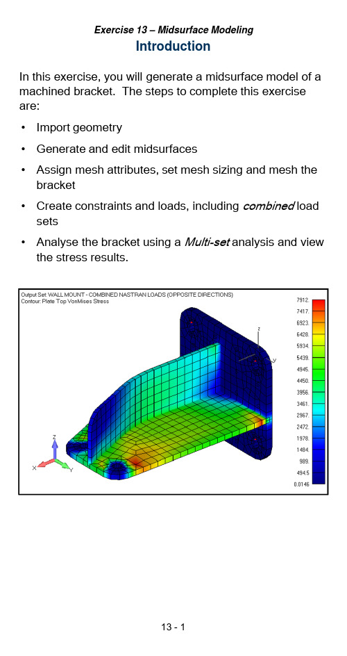
IntroductionIn this exercise, you will generate a midsurface model of a machined bracket. The steps to complete this exercise are:•Import geometry•Generate and edit midsurfaces•Assign mesh attributes, set mesh sizing and mesh the bracket•Create constraints and loads, including combined load sets•Analyse the bracket using a Multi-set analysis and view the stress results.Step 1:Import geometryImport the Parasolid geometry of the multi-thickness solid model.•Open a new FEMAP model.•Select the File, Import, Geometry command.•Select the Parasolid file ex13-Bracket_inches.x_t from your class Geometry folder.•Click OK to accept the defaults in the Solid Model Read Options dialog box.Change the view orientation to the Trimetric view.•Press the F8key (or use the View, Rotate, Model command) to open the View Rotate dialog box.•Select the Isometric button.•Click OK to close the dialog box.Save the model•Save the model in your class Exercises folder as “ex13-Bracket.modfem”.Step 2:Create midsurfacesExtract the midsurfaces from the solid.•Select the Geometry, Midsurface, Automaticcommand.•Click the Select All button to select all the surfaces on the solid.•In the Mid-Surface Tolerance dialog box, click the Measure Distance icon to enable measuring a 3-Ddistance. Ctrl+D can also be used to measure adistance from the graphics window while in acommand.•When the Locate –Define Location to Measure From dialog box is displayed, select one of the points onthe thickest edge of the sold. Set the Method to OnPoint and select one of the points shown below.•Click OK to confirm the selection of the first point.•Select the “other” point shown below that has not been chosen, then click OK to confirm the selection.•Click OK to accept the calculated distance, .156 in the Mid-Surface Tolerance dialog box. FEMAP willnow extract the mid-surfaces.Display the automatically generated Midsurfaces group.•In the Model Info pane, turn on “highlighting” by clicking the Show When Selected icon.•Expand the Group object in the tree and select1..Midsurfaces in the Model Info pane. This willhighlight the newly created group. Since we are onlyworking with a single part, you can delete the groupand the original solid.•Right-click 1..Midsurfaces and select Delete from the context-sensitive menu.•Expand the Geometry object in the Model Info tree, select 1..ex12-Bracket, and using the context-sensitive menu, Delete the original solid part.•Expand the view if needed with the Ctrl+A hotkey to “Autoscale”Note that the midsurfacing operation has generatedsplit lines in the midsurfaces that will be easily beremoved in the next step.Remove the split lines from the surfaces.•Select the command, Geometry, Solid, Cleanup.•Select All surfaces and click OK.•In the Solid Cleanup dialog box, accept the default option to Remove Redundant Surfaces and click OKto proceed with remove the split lines in the surfaces.Extend the surface representing the bend of the rib.•Switch your view orientation to the Front view.•Note that the bottom edge of bend surface doesnot intersect the surface representing the flange.•Select the command, Geometry, Midsurface, Extend.•Select the bottom edge of the bend surface in the Select Entity dialog box.Complete extending the surface representing the bend of the rib.•In the Surface Extend Options dialog box, leave the option for Extend Shape as Linear.•Using the Extend To –Solid option, select the Solid that represents the flange and click OK.Note that the blend surface now extends to theintersection with the flange.Trim the two surfaces representing the flat sections of the rib.You will use two different Geometry, Midsurfacecommands to do this, the first is to use the Trim with Curve operation and the second is use the Intersect operation.•Select the command, Geometry, Midsurface, Trim with Curve.•Select the flat surface of the rib closest to the back surface (the surface with the four mounting holes) inthe Solid/Surface to Trim dialog box and the clickOK.•In the Entity Select ion –Select Line(s) to Trim With dialog box, select the top edge of the rib and theedge of the blend surface intersecting the flat ribsection and click OK to confirm your selection.•With highlighting enabled in the Model Info pane, select the sheet solid of the rib section you justmodified and note how it has been sliced into threesurfaces.Continue with trimming the two surfaces representing the flat sections of the rib.•Select the command, Geometry, Midsurface, Intersect.•Select the two (2) surfaces that will represent the blend and the end of the rib then click OK togenerate the intersection.Delete the extraneous surfaces.•Select the command Delete, Geometry, Surfaces.•Select the small tab on the longer flat section of the rib and the two surfaces on the flat rib sections thatextend beyond the blend of the rib. Click OK todelete the surfaces.Stitch the surfaces together to create contiguous sheet solids.•Select the command Geometry, Solid, Stitch.•Select all the surfaces and click OK.•Click OK to accept the default Gap Tolerance.•Note how there are now three sheet solidsrepresenting the back face, web, and rib of thebracket.Intersect the surfaces to imprint the surfaces at the intersection of the three main features of the bracket.•Select the command Geometry, Midsurfaces, Intersect.•Select all the surfaces and click OK.•Again, using the Model Info pane, click the three sheet solids under the Geometry tree and note howthe surfaces have been imprinted using theintersection operation.Create Offset Curves around the six holes on thebracket.•If not displayed, active the Curves on Surfaces toolbar.•Click the Curve Washer icon on the Curves on Surfaces toolbar.•In the Define Washer or Offset Curves dialog box,set the Mode to Washer , enable the option for Save Split Lines and set the Offset to .125. Click OK to accept the settings.•Select one of the arcs on each of the six holes on thebracket and click OK .•Cancel out of the Curve Washer command.•After completing the Curve Washer operation, your model should appear as follows (shown with multiple windows to more clearly display the washers).Step 3:Assign mesh attributes, set mesh sizing and mesh the bracketAssign the mesh attributes (property) to themidsurfaces.•Select the Geometry, Midsurface, Assign Mesh Attributes command.•Press Select All the surfaces and click OK.•The Define Material –ISOTROPIC dialog box will open, prompting you for a material. Click the Loadbutton to open up the default material library.•In the Select from Library dialog box, select one of the Stainless Steel materials and click OK.•Click OK.•In the dialog box, click Yes to consolidate the properties by thickness.•Note that there are now two (2) properties that reflect the two different wall thicknesses of the part.Set the mesh size for the mid-surfaces.•Using the Select toolbar, set the Selector Entity to Surface and Selector Mode to Select Multiple .•Select all the surfaces by holding down the Shift keyto create a box picking region around the entire model.•In the graphics pane, right-click your mouse andselect Mesh Size from the context-sensitive menu.•In the Automatic Mesh Sizing dialog box, set the Element Size to .2 set the Max Angle Tolerance to15. Disable the Max Elem on Small Feature optionthen click OK to set the mesh size.Set the mesh size for the curves around the holes•Before meshing, turn on the mesh size indicators using the F6hotkey to open the View Options dialog box.•In the View Options dialog box, set the Category to Labels ,Entities and Color, enable the Draw Entityoption and set Show As to 3..Symbols and Count.Click Apply to update the display and once theoptions are displayed as below, you can close thedialog box by clicking either the OK or Cancelbutton.Set mesh sizes for the holes.•Using the Select toolbar, set the Selector Entity to Curve and leave the Selector Mode as SelectMultiple.•Select the curves surrounding the holes on the bracket to include the hole and the washer’s arcs,but not the split lines.•In the Model Info pane, expand the Selection List object .•Right-click the Curves object and select Mesh Size from the context-sensitive menu.•In the Mesh Size Along Curve dialog box, set the Number of Elements to 6 then click OK to set themesh size.Mesh the model.•In the Model Info pane, right –click the Surfaces object then select Mesh from the context-sensitivemenu.•Click OK in the Automesh Surfaces dialog box to mesh the model using the “Mesh Attributes”assigned to the surfaces in an earlier step.With mesh size symbols turned off and elementthickness display turned off, your model shouldappear similar to the following.Step 4:Create constraints and loads, including aCombined load setCreate the constraints on the back wall of the part.•In the Model Info pane, create a Constrain Set. Use a descriptive name for the title of the constraint set.•Expand the new constraint set and right-clickConstraint Definitions and select On Surface from the context-sensitive menu.•Select the eight (8) surfaces which represent the washers around the holes on the back wall of the bracket.•In the Create Constraints on Geometry dialog box,set the constraint to Pinned then click OK to create the constraints.•Again, right-click Constraint Definitions and select On Surface from the context-sensitive menu.Continue with creating the constraints on the back wall of the bracket.•Select the two (2) remaining surfaces on the back wall of the bracket and click OK.•In the Create Constraints on Geometry dialog box, set the constraint to Surface and choose Slidingalong Surface (Symmetry)then click OK to create the constraints.Create the loads on the holes on the left end of the bracket. To do this, you will create a Rigid elementconnecting the washers of the holes on the front of the bracket to a node at the center of the holes.•Select the command, Model, Element.•In the Define Plate Element dialog box, click the Type button an d select the Rigid element under theOther type.•Click the RBE2tab.•Click the New Node at Center button. Femap will then create the Independent node at the center ofthe selected Dependent nodes.•Click the Nodes button.•In the Entity Selection dialog box, change Methods^to on Curve and select the two curves making up one of the two holes on the web then Click OK to confirm your selection.•Create a second rigid element on the other hole byrepeating the previous two steps (New Node atCenter and selecting nodes on the two curves on the edge of the other hole).Create loads on the center nodes of the rigid “spider”elements in the holes.•Zoom in on the end of the bracket where you just created the rigid “spiders”.•From the Model Info tree, right-click the Loads object select New .•Enter a Title for the new Load Set as Front Web Hole Loading and click OK .•Expand the Load Set just created, right-click Load Definitions and select Nodal from the menu.•Select the node at the center of the front hole rigid element on the web then click OK .•In the Create Loads on Nodes dialog box, enter adescriptive name for the load, set the Load Type to Force , and set the Load value to FZ = 1.•Create a second load set and load at the node at the center of the read hole on the web by repeating steps b) through f) for the other hole. Set the Title for the second load set to Rear Web Hole Loading and click OK .Create a combined load set that will take the two previous load sets and by setting a scale factor, willcreate a combined load of 100 lbs in the negative Zdirection.•Select the command Model, Load, Combine.•In the Combine Load Data dialog box, set the Title to Combined 100 lb Web Hole Load.•In the From list, select both of the load sets you just created.•With both load sets selected, set the Scale Factor to -50.•Click the Add Combination button.•After the previous step, the Combinations section of the dialog box should appear as shown to the right.•Click OK to create the combined load set.•In the Model Info pane, right-click the combined load set you created and select Activate from the menu. Create a Nastran combined load set that will take the two previous load sets and by setting a scale factor, will create a combined load of 50 lbs in the positive Zdirection for the front hole and 50 lbs in the negative Z direction for the rear hole.•In the Model Info pane, right-click the Loads object and select New from the menu.•In the New Load Set dialog box, set the Title to a descriptive name similar to below.•For the Set Type, select Nastran LOAD Combination then click OK.•Select Reference Sets after right-clicking the newly created load set in the Model Info pane.•In the Referenced Loads Sets for Nastran LOAD dialog box, click the first load set under the Available Sets list field.•With the first load set selected, set the value For Referenced Set to 50then click the Add Referenced Set button.•With the second load set selected, set the value For Referenced Set to -50 then click the Add Referenced Set button. The Referenced Sets list field shouldappear as below.•Click OK to update the load set.Display the element thickness.•From the View toolbar, select the View Style pull down icon and select the Thickness/Cross Sectionicon to toggle on the display of the elementthickness.Step 5:Analyze the bracket and display stress resultsModify the Femap preference for Output Set Titles .•Select the command File, Preferences .•Select the Interfaces tab.•Under the Nastran Solver Write Options group, setthe Output Set Title option to 2..Nastran SUBTITLE .•Click OK to apply the changes to Femap’s preferences.Create an MultiSet Analysis Set and run the analysis.•Create an new analysis set for NX Nastran Linear Statics by right-clicking the Analysis object in theModel Info pane and select New.•Set the Title of the analysis set to MultiSet Linear Statics.•Expand the newly created analysis set to display Boundary Conditions.•Select Boundary Conditions then click Edit.Continue with creating the new analysis set for linear statics.•Set both the Constraints and Loads to None.•Click the MultiSet button.•In the Entity Selection –Select Constraint Set(s) to Generate Cases dialog box, click Select All thenOK.•In the Entity Selection –Select Load Set(s) to Generate Cases dialog box, click the Select fromList button.•In the Select One or More Load Sets(s) dialog box, select the two combined load sets, then clickOK.•Click OK to add the two load sets to the analysisset. The analysis set should now show two subcases as part of the analysis set.•Click the Analyze button in the Analysis Set Manager dialog box to start the analysis.•Close the NX Nastran Analysis Monitor when theanalysis completes and the results sets have been read into Femap.Review the results.•Activate the first results set by right-clicking on it in the Model Info pane.•Using the PostProcessing Toolbox, create a deformed contour plot of the Plate TopMajorPrin(cipal)Stress.•Set the Type to Elemental•Enable the option for Double-Sided Planar.•Save your model and exit Femap.。
Sec03_几何建模

S3-12
案例学习:简单实体的拓朴
由参数化实体创建参数化面, 例如一个面的位置 u=0.5
Set Action/Object/Method to Create/Surface/Extract. Set the u Parametric Value to 0.5. Select Solid 1 for Solid List. Apply. 将设置改为v=0.5 ,w=0.5,重复操作.
P 3
1
P 4 Y
Z
X
PAT301, Section 3, October 2004 Copyright 2004 MSC.Software Corporation
S3-21
几何创建(续)
复杂体
复杂或非参数化体 (N个面) (白色)
非参数化实体可以是 Patran 本身的 B-Rep (边界表征) 或 parasolid B-Rep CAD 体可以被转化成 Patran 本身的 B-Rep 或 parasolid B-Rep 体, 然后用自动的TetMesh算法生成网格
S3-9
案例学习:简单实体的拓朴
然后,看体的边 例如 Solid 1.2.3
PAT301, Section 3, October 2004 Copyright 2004 MSC.Software Corporation
S3-10
案例学习:简单实体的拓朴
先删掉Point 7,再在体的顶点上创建一个点.
先用三角形划分面, 然后用四面体划分体 类似 Paver 网格生成器
B-Rep Solid
Tetrahedral Mesh
PAT301, Section 3, October 2004 Copyright 2004 MSC.Software Corporation
山东交通学院本科生毕业论文

为深入分析某轻型汽车车桥的桥体静态振动强度和车桥振动响应特性,运用新型有限元矢量分析法对它车桥进行矢量数值分析模拟。
采用一种有限元特性分析计算工具利用ANSYS对三种不同工况下的车桥结构进行了三种静态运动强度的特性分析,并对它们的三种动态强度特性分别进行了自由模态的特性分析。
应用有限数值单元运算法对它的数值进行运算模拟。
即:静力分析和动态分析中的网格可对局部进行加密,模态分析的数据良好,较为均匀,达到了理想程度。
从数据上看,静运动达到了合理水平,能够保证汽车车桥在设计时的性能要求。
通过数据分析实验结果明确表明,车桥主体结构的静运动特性和受力的变化特性基本都保证了车桥在设计中的一系列要求。
从而能够更好的设计车桥结构,并且让它具有好的静力特性和动态特性。
关键词:ANSYS,车桥,有限元,模态分析In order to deeply analyze the static vibration intensity and response characteristics of a light truck bridge, the new finite element vector analysis method is used to simulate its vehicle bridge. In this paper, a finite element analysis tool is used to analyze the characteristics of three kinds of static motion strength of vehicle bridge structure under three different working conditions by ANSYS, and the characteristics of three kinds of dynamic strength characteristics of them are analyzed by free mode. The finite element method is used to simulate its numerical value. That is to say, the mesh in static analysis and dynamic analysis can encrypt the local part, and the data of modal analysis is good and even, reaching the ideal degree. From the data point of view, the static motion has reached a reasonable level, which can ensure the performance requirements of the automobile axle in the design. Through the data analysis and experiment results, it is clear that the static and dynamic characteristics of the main structure of the axle and the changing characteristics of the force basically ensure a series of requirements in the design of the axle. So it can better design the axle structure, and make it have good static and dynamic characteristics.Key words:ANSYS, bridge, finite element, modal analysis前言 (1)1绪论 (2)1.1概述 (2)1.1.1国内外发展的状况及现状的介绍 (2)1.2 车型简介 (3)1.3 有限元方法简介 (3)1.3.1有限元法的基本原理 (3)1.4 ANSYS简介 (4)2车桥模型的建立 (5)2.1车桥单元类型的选取 (5)2.2 车桥模型的基本要求 (5)2.3 有限元建模方法的选择 (5)2.4模型简化 (6)3车桥静态分析 (7)3.1静态分析的基础 (7)3.2静力分析关系装配处理方法 (7)3.3操作台结构网格划分 (7)3.4边界条件与载荷的确定与施加 (8)3.4.1施加边界条件 (9)3.5分析和读取计算结果 (9)4车桥的模态分析 (10)4.1模态分析简介 (10)4.2模态的分析 (10)结论 (14)致谢 (15)参考文献 (16)附录 (17)有限元分析法在国内以及国外的汽车数值分析技术方面的运用和研究状况:有限元的单元运算法其实是一种很有效的汽车数值图形计算分析方法,它不仅能对帮助工程师在实际中发现几何体的形状不规则。
Geometric Modeling

Geometric ModelingGeometric modeling is a crucial aspect of computer graphics and design, allowing for the creation of three-dimensional representations of objects and scenes. It involves the use of mathematical equations and algorithms to define the shape, size, and position of objects in a virtual space. Geometric modeling isused in a wide range of applications, including animation, video games, architectural design, and engineering. One of the key benefits of geometric modeling is its ability to create realistic and detailed representations of objects. By accurately defining the geometry of an object, designers can create lifelike images that closely resemble the real world. This level of detail is essential for applications such as architectural design, where precise measurements and proportions are crucial. In addition to creating realistic images, geometric modeling also allows for the manipulation and transformation of objects in a virtual space. Designers can easily modify the size, shape, and position of objects, allowing for quick iterations and adjustments during the design process. This flexibility is particularly valuable in fields such as industrial design and engineering, where multiple design iterations are common. Another important aspect of geometric modeling is its ability to simulate physical phenomena and interactions. By accurately modeling the geometry of objects andtheir relationships, designers can simulate how objects will behave in different environments and under various conditions. This is essential for applications such as virtual prototyping and simulation, where designers need to test the performance of a design before it is physically built. Geometric modeling also plays a crucial role in computer-aided design (CAD) and computer-aided manufacturing (CAM) processes. By accurately defining the geometry of objects, designers can create detailed blueprints and specifications that can be used to manufacture physical objects. This level of precision is essential for industries such as aerospace and automotive, where small errors in design can havesignificant consequences. Overall, geometric modeling is a powerful tool that enables designers and engineers to create realistic, detailed, and accurate representations of objects in a virtual space. By leveraging mathematicalequations and algorithms, designers can create lifelike images, manipulate objects,simulate physical interactions, and generate detailed specifications for manufacturing. As technology continues to advance, geometric modeling will continue to play a crucial role in a wide range of industries and applications.。
关于半挂车车架有限元分析与轻量化分析
关于半挂车车架有限元分析与轻量化分析摘要:文章主要从半挂车实体建模及有限元的简述出发,分别简述了车架有限元模型的建立,以及轻量化的车架结构优化,旨在与广大同行共同探讨学习。
关键词:半挂车车架;有限元分析;轻量化一、半挂车实体建模及有限元的简述1.半挂车介绍半挂车是一种道路运输车辆,由两部分构成,一部分是带有动力的车头,另一部分为承载货物的半挂。
半挂车是目前普遍应用的运输工具,按用途分为专用和普通两种。
按大梁的结构来分有平板式、阶梯式、凹梁式三种。
如下图1-1所示。
图1-1 半挂车分类板式半挂车可以最大利用空间,同时离地面较高,方便公路运输。
阶梯式半挂车货台比较低,方便货物的装卸,凹梁式半挂车具有较小的离地间隙和较低的货台。
半挂车第二部分半挂结构主要由车架、双侧保护装置、工具箱、挡泥板、轮轴、牵引装置、电路、气制动、支撑、悬架装置、备胎、车箱、后保险杠等结构组成。
2.有限元法介绍有限元法是用简单的问题替换复杂的问题并进行求解,具有计算精度较高的优点,可对不同复杂形状的工程问题进行科学有效的分析以及计算。
二、车架有限元模型的建立建立有限元模型是进行有限元分析的基础,也即选择单元类型、赋予材料属性、划分网格、模拟连接方式、施加边界条件的过程,其中划分网格是前处理最为重要也是最为繁琐的步骤。
1.建立车架有限元模型应遵循的原则(1)确保模型的计算效率。
网格的大小、稀疏程度,也即单元与节点的数目多少,决定着计算结果的准确性和计算效率,在进行车架有限元模型建立的过程中应权衡好计算结果的准确性与计算效率的矛盾,找到最合适的网格尺寸。
(2)确保计算结果的准确性。
建立车架三维几何模型的过程中,在不影响分析结果的前提下,已经对车架进行了一定的简化,目的就是为了能够得到准确的结果,避免造成应力集中等问题。
2.模型导入及中面抽取(1)三维几何模型的导入和修复我们将利用 Solidworks 软件建立的车架的三维几何模型导入 Hypermesh 中。
COMSOL Multiphysics-几何建模-0822
旋转 拉伸 合集
旋转
合集
旋转 合集
仿 真 智 领 创 新
Simulating inspires innovation
创建3D几何模型
新增xy工作平面
拉伸 合集
新增xy工作平面 阵列 拉伸
仿 真 智 领 创 新
Simulating inspires innovation
创建3D几何模型
仿 真 智 领 创 新
Simulating inspires innovation
端盖面
将开放的空间封闭,从而 形成求解域
仿 真 智 领 创 新
Simulating inspires innovation
端盖面
• 端盖流道末端,随后剖分CAD导入部分的内部区域.
• 通过选择边界描绘出所围面区域.
消除和修复操作
仿 真 智 领 创 新
Simulating inspires innovation
消除和修复操作
模型路径: C:\ProgramFiles\COMSOL\COMSOL43 \models\CAD_Import_Module\ Tutorial_Models\defeaturing_demo_ 6.x_b
Creating a 2D Geometry Model
仿 真 智 领 创 新
Simulating inspires innovation
创建2D几何模型
定义几何扫描参数
仿 真 智 领 创 新
Simulating inspires innovation
创建2D几何模型
绘制两个圆
布尔运算:差集
增加矩形
仿 真 智 领 创 新
Simulating inspires innovation
西门子PLM软件NX数字模拟产品功能说明书
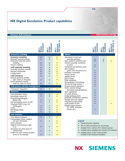
Legend•Standard product capability#Part of CAD prerequisite for this packageP Available from a Siemens PLM Software partnerA Available add-on capability from Siemens PLM Software A*Available add-on to NX ®Advanced FEM.Included in NX Advanced SimulationNX Digital Simulation:Product capabilitiesNX/ugsSiemens PLM Software MotionAssociation to part and assembly geometry##Basic motion in assembly task ##•Convert assembly constraints to joints•Mechanical and primitive joints •Joint couplers(gears,rack and pinion etc.)•Kinematic constraints •Motion drivers •Applied forces •Joint Friction •Initial conditions•Spring/damper and bushings •2D and 3D body contact •General function operators •Driver control througharticulation and spreadsheet •Static equilibrium •XY graph plotting •Design packaging tools•Kinematic and dynamic solutions •Multiple load case support •Integrated postprocessor •Load transfer to FEA ••Mutiple output formats (JT,VRML,animation movies,etc.)•N X 5D e s i g n S i m u l a t i o nN X 5A d v a n c e d F E M (M a c h 2)N X 5M o t i o n S i m u l a t i o nN X 5M o t i o n S i m u l a t i o nN X 5D e s i g n S i m u l a t i o nN X 5A d v a n c e d F E M (M a c h 2)Geometry modelingGeometry modeling##•Parasolid ®geometry kernal ##•Parametric solid and surface modeling##•Feature modeling##•CAD assembly modeling##•Assembly structure creation ##•Interpart relationship ##•Configurations##•CAD interfaces##•Neutral geometry transfer IGES,STEP,JT,Parasolid ##•Direct geometry transfer Catia V4,Catia V5,Pro/EPPPCAE process and data management Teamcenter ®integration •••OpennessCAD parameter access •••Recordable session file •••Programming/debugging session files•••Full functionality access via API •••Integrated BASIC prog.env.w/debugging •••HTML•••Knowledge Fusion •••WAVE •#•User interfaceUser defined templates•••Customizable menus,toolbars and user commands •••Smart selection•Support external plug-in apps in UI•••Interactive (no-click)query of model/results•••Model tree with context sensitive access to functionality•••N X 5D e s i g n S i m u l a t i o nN X 5A d v a n c e d F E M (M a c h 2)N X 5D e s i g n S i m u l a t i o nN X 5A d v a n c e d F E M (M a c h 2)FE model building Geometry defeature tools –topologydiagnosis,geometry repair,CAD featuresuppression,stitch surface,remove hole/fillet,partition••Non-manifold topology generation for volumes•CAE topology•CAE geometry –creation and deletion,mid-surfacing (constant and variable thicknesses)•Automatic topology abstraction –abstraction control,auto stitch geometry,auto merge small regions,auto pinch••Manual topology modification tools•Meshing••0D,1D,and 2D elements •2D mapped meshing •3D elements••Automatic meshing asst.–geometric abstraction and mesh generation in one tool/step ••Batch meshing •Transition meshing•Manual meshing tools –sweeping,revolve,surface coating,interactive controls,etc.•Automatic meshing controls –local element sizing,curvature control•General modeling tools••Axi-symmetric meshing•Mesh display and control –display filters••Material property creation and management –isotropic,anisotropic,orthotropic,linear,nonlinear,thermal,etc.••Mass property calculations •Load summation•Physical property creation and management ••Mesh quality checks –coincident nodes,free edge checks,element shape checks,etc.••FE grouping –by association to geometry,bc’s,material,etc.)•FE collectors and sets •FE append•FEM on assembly••FE model on CAD assembly••Beam modeling•Model update from CAD••FEM model update based on geometry change ••FEM model update based on assembly change••FE model buildingBoundary conditions••Application methods ••On geometry••Local coordinate system ••On FE entities •Friction definition •Time variation•Constraints –statics,dynamics,thermal,symmetric,contact,etc.••Structural loads••Structural thermal –flux,radiation,generation••Advanced thermal –convection,temperature –linear and nonlinear,simple radiation,thermal coupling,adv.radiation•Flow –bc’s,flow surface/blockage/screen definition,fluid domain definition •Axi-symmetric boundary conditions •Automatic contact detection and setup ••Automated load transfer •Laminate composites ASolution setupStructural linearStatic and buckling analysis••Structural linear dynamicsNormal modes••Direct frequency response •Direct transient response •Modal frequency response •Modal transient response•Structural nonlinearStatic,transient,geometric,elastic/plastic material ••Implicit solver •Explicit solver•Structural contact and connection modelingSurface-to-surface contact ••Node-to-node contact •Rigid elements•Constraint elements •Glue connection••ThermalSteady-state•Diurnal solar heatingA Rigid-body transient motion A Transient A Conduction A Convection A RadiationAN X 5D e s i g n S i m u l a t i o nN X 5A d v a n c e d F E M (M a c h 2)N X 5D e s i g n S i m u l a t i o nN X 5A d v a n c e d F E M (M a c h 2)Solution setup Fluid dynamicsSteady-state/transient flow A Incompressible flow A Compressible flow A Laminar/turbulent flow A Internal/external flow A Motion-induced flowA Multiple rotational frames of reference A Forced and natural convectionA Conjugate and radiation heat transferACoupled physicsThermal-structural •A Fluid-thermalA FE data export••Abaqus (inp)A Ansys A Nastran•A*FE data import••Abaqus (fil,inp)A Ansys (rst)A Nastran (op2,dat)•A*NX I-deas ®(unv,afu,bun)•FE results visualizationContour displays (continuous or iso-lines)••Vector displays ••Isosurface displays ••Cutting planes••Advanced lighting control ••Animations••Complex dynamic response results •Multiple viewports••Probing of results on nodes••Postprocessing data table w/sort/criteria ••Results listings••Transparency display ••Local coordinate system ••XY graphing•Synchronized contour and XY plotting displays •Annotated graphs•Output (JT,VMRL,postscript,tif,etc.)••Meta solutionDurability••FE parameter optimization••Dynamic forced response simulation A Laminate composites analysisAN X N a s t r a nN X M u l t i -p h y s i c sN X N a s t r a nN X M u l t i -p h y s i c sSolutions Structural linearStatic •Modal •Buckling•Structural nonlinearStatic •Transient •Geometric•Elastic/plastic material •Hyperelastic material •Gasket material •Nonlinear buckling •Implicit solver •Explicit solver•Structural contact and connection modelingSurface-to-surface contact •Node-to-node contact •Spot welds •Rigid elements•Constraint elements •Glue connection•Structural linear dynamicsModal transient •Modal frequency •Direct transient •Direct frequency •Shock spectrum •Random vibration •Rotor dynamics•ThermalSteady-state,transient••Temperature-dependent properties ••Nonlinear thermal contact•Thermal couplings (welded,bolted,bonded)•Disjoint meshes support in assembly modeling•Surface-to-surface radiative heat transfer ••Hemicube-based view factor calculation •Radiation in participating media •Radiation enclosures•Environmental radiative heating •Orbital modeling and analysis •Specular,transmissive surfaces ••Convection••Forced and natural convection correlations •Hydraulic fluid networks •Joule heating •Phase change•Heater and thermostat modeling ••Material charring and ablation •Transient rigid body motion •Peltier cooler modeling•Heat sink models and modeler•PCB modeler/xchange (ECAD/MCAD)ASolutionsFluid dynamicsSteady-state/transient flow •Incompressible flow •Compressible flow •Laminar/turbulent flow•Forced and natural convection•Conjugate and radiation heat transfer •Porous media modeling •Nonlinear fluid properties •Humidity and condensation•Automatic fluid domain and boundary layer meshing•Flow induced by rigid body motion •Automated connection of disjoint fluid meshes •Fan models•Embedded 2D/3D flow blockages •General scalars and particle tracking •Non-Newtonian fluids•Multiple rotating frames-of-reference•Coupled physicsAcoustics•Acoustics-structural •Subsonic aeroelastic •Supersonic aeroelastic •Fluid-thermal•Thermal-structural ••Fluid-structural•Interface to multi-body dynamics (ADAMS and RecurDyn)•SolversIterative ••Sparse direct•Shared memory processing •Distributed memory processing •(1)•Optimization ••Cyclic symmetry ••Axi-symmetric••FE-based finite volume solver•Advanced capabilitySuperelement/substructuring ••Solution customization (DMAP)•Solution customization (user subroutine)•(1)Available in Enterprise versions only.Note:The NX Nastran and NX Multi-Physics solver suites are comprised of multiple products.Please check the individual product fact sheets to determine the simulation capabilities contained in each core bundle or add-on module.ContactSiemens PLM SoftwareAmericas8004985351Europe+44(0)1276702000Asia-Pacific852********/plm©2007.Siemens Product Lifecycle Management Software Inc.All rights reserved.Siemens and the Siemens logo are registered trademarks of Siemens AG. Teamcenter,NX,Solid Edge,Tecnomatix,Parasolid,Femap,I-deas,JT,UGS Velocity Series,Geolus and the Signs of Innovation trade dress are trademarks or registered trademarks of Siemens Product Lifecycle Management Software Inc.or its subsidiaries in the United States and in other countries.All other logos,trademarks,registered trademarks or service marks used herein are the property of their respective holders.9/07。
Patran基础教程03_几何建模
PAT301, Section 3, September 2010 Copyright 2010 MSC.Software Corporation
S3-11
案例学习:简单实体的拓扑
● 现在通过擦除实体来观察体中的参数化面.
● Display/Plot/Erase. ● Enter Solid 1 for Selected Entities. ● Erase.
no?导入的几何将不会是parasolid格式而是sgm几何mscpatrannativesolidgeometrymodel?entitylayers?所有层或选择的层被导入?groupclassification?显示对话框来指导实体进入mscpatran组?creategroupsfromlayers?自动由cad层创建mscpatran组?groupname
S3-2
拓扑结构
● ●
Patran 结合拓扑结构来定义几何 Patran 中的拓扑实体是
Face
Vertex Body
Edge
● ●
角点保留了边, 面, 体的位置 在Patran语法中,所有的拓扑元素都是可以被光标选取的 (例如 Surface 10.2)
S3-3
PAT301, Section 3, September 2010 Copyright 2010 MSC.Software Corporation
第 3部分 几何建模
PAT301, Section 3, September 2010 Copyright 2010 MSC.Software Corporation
S3-1
基本概念
PAT301, Section 3, September 2010 Copyright 2010 MSC.Software Corporation
ICEM CFD划分网格(百度经验)
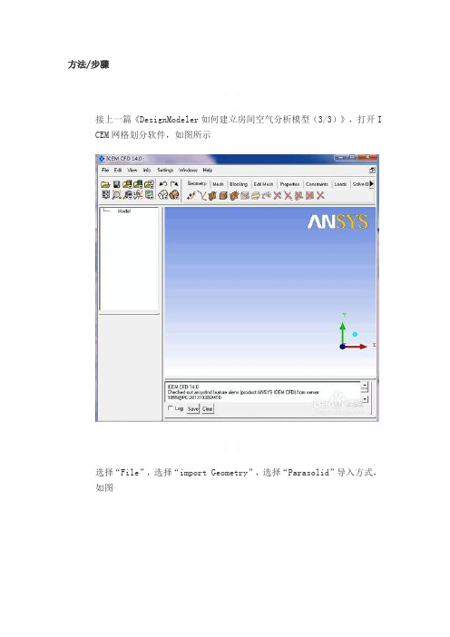
方法/步骤1. 1接上一篇《DesignModeler如何建立房间空气分析模型(3/3)》,打开I CEM网格划分软件,如图所示2. 2选择“File”,选择“import Geometry”,选择“Parasolid”导入方式,如图3. 3打开上一篇已经保存的房价分析模型,如图所示4. 4打开之后,叫你选择单位,这里选择“milimeter”单位,如图所示5. 5 点击“ok”按钮,如图6. 6弹出如图所示对话框(我这里是以前有相同名字的文件划分过网格),点击“yes”按钮,如图7.7然后又弹出一个窗口,问你是否要创建新project,选择“yes”,如图所示8.8模型就已经导入ICEM中了,按住鼠标左键旋转模型,如图所示9.9展开“Model”中的“parts”,如图所示10.10右键单击“parts”,选择“Create Part”,如图所示11.11 出现如图所示对话框12.12在“part”对话框中输入“INLET”,如图所示13.13展开“Geometry”,勾选“surface”,如图所示14.14选择“create part by selection”中“Entities”右边的鼠标箭头,如图15.15 出现如图所示对话框,16.16由于篇幅过大,图片过多。
第二部分《ICEM-CFD如何划分网格》分为五篇文章发出来,分别为:《ICEM-CFD如何划分网格(1/5)》,《ICEM-C FD如何划分网格(2/5)》,《ICEM-CFD如何划分网格(3/5)》,《IC EM-CFD如何划分网格(4/5)》,《ICEM-CFD如何划分网格(5/5)》.方法/步骤1. 1接上一篇《ICEM-CFD如何划分网格(1/5)》,选择空调进风口面,作为“INLET”,准备创建进口边界面,如图所示。
2. 2选中之后按鼠标中间或者“ok”按钮,“parts”栏中已经出现“INLET”了,如图3. 3再在“create part”中输入“OUTLET”,准备创建出口边界面,如图所示4. 4选择“create part by selection”中“Entities”右边的鼠标箭头,如图5. 5选择出风口面,作为“OUTLET”,准备创建出口边界面,如图所示。
中南大学学报论文

Foundation item: Project(50678059) supported by the National Natural Science Foundation of China Received date: 2008−06−25; Accepted date: 2008−08−05 Corresponding author: ZHU Qing-jie, Professor, PhD; Tel: +86−315−2616969, +86−13932521086; E-mail: qjzhu@
J. Cent. South Univ. Technol. (2008) 15(s1): 307−310 DOI: 10.1007/s11771−008−369−0
Finite element analysis of fluid-structure interaction in buried liquid-conveying pipeline
Abstract: Long distance buried liquid-conveying pipeline is inevitable to cross faults and under earthquake action, it is necessary to calculate fluid-structure interaction(FSI) in finite element analysis under pipe-soil interaction. Under multi-action of site, fault movement and earthquake, finite element model of buried liquid-conveying pipeline for the calculation of fluid structure interaction was constructed through combinative application of ADINA-parasolid and ADINA-native modeling methods, and the direct computing method of two-way fluid-structure coupling was introduced. The methods of solid and fluid modeling were analyzed, pipe-soil friction was defined in solid model, and special flow assumption and fluid structure interface condition were defined in fluid model. Earthquake load, gravity and displacement of fault movement were applied, also model preferences. Finite element research on the damage of buried liquid-conveying pipeline was carried out through computing fluid-structure coupling. The influences of pipe-soil friction coefficient, fault-pipe angle, and liquid density on axial stress of pipeline were analyzed, and optimum parameters were proposed for the protection of buried liquid-conveying pipeline. Key words: fluid-structure coupling; buried liquid-conveying pipeline; ADINA; finite element; faults; earthquake
NX 8.0 模拟产品功能概述说明书

•
•
#
#
#
#
#
#
#
#
#
#
#
•
•
#
#
#
#
#
#
#
#
#
#
#
•
•
#
#
#
#
#
#
#
#
#
#
#
•
•
#
#
#
#
#
#
#
#
#
#
#
•
•
#
#
#
#
#
#
#
#
#
#
#
•
•
#
#
#
#
#
#
#
#
#
#
#
•
•
#
#
#
#
#
#
#
#
#
#
#
•
•
#
#
#
#
#
#
#
#
#
#
#
•
•
#
#
#
#
#
#
#
#
#
#
#
•
•
#
#
#
#
#
#
#
#
#
#
#
•
•
#
#
#
#
#
#
#
#
#
#
#
•
•
#
#
#
#
#
#
#
#
#
#
#
【方向】ICEM笔记

【关键字】方向目录5.2.3 Extend Split (17)5.2.4 Split Face (17)5.2.5 Split Vertices (17)5.3 Merge V ertices (17)5.3.1 Merge Vertices (17)5.3.2 Merge Vertices By Tolerance (18)5.3.3 Collapse Block (18)5.3.4 Merge Vertex To Edge (18)5.4 Edit Block (19)5.4.1 Merge Blocks (19)5.4.2 Merge Faces (19)5.4.3 Modify Ogrid (20)5.4.4 Periodic Vertices (20)5.4.5 Convert Block Type (20)5.4.6 Change Block IJK (21)5.4.7 Renumber Blocks (21)5.5 Associate (21)5.5.1 关联经验 (21)5.5.2 Associate Edge To Curve (22)5.5.3 Associate Face to Surface (22)5.5.4 Disassociate from Geometry (22)5.5.5 Update Associations (22)5.5.6 Reset Project Vertices (22)5.5.7 Snap Project Vertices (23)5.5.8 Group/Ungroup Curves (23)5.5.9 Auto Associate (23)5.6 Move Vertex (23)5.6.1 Move Vertex (23)5.6.2 Set Location (23)5.6.3 Align V ertices (23)5.6.4 Align V ertices In-line (24)5.6.5 Set Edge Length (24)5.6.6 Move Face Vertices (24)5.7 Transform Blocks (24)5.8 Edit Edge (25)5.8.1 Split Edge选项 (25)5.8.2 Unsplit Splits选项 (25)5.8.3 Link Edge选项 (25)5.8.4 Unlink Edge (26)5.8.5 Change Edge Split Type (26)5.9 Pre-mesh Params (27)5.9.1 Update Sizes (27)5.9.2 Scale Sizes (27)5.9.3 Edge Params (27)5.9.4 Edge Params中的Link bunching如何使用,按照help做没成功。
comosol 3.5功能说明

COMSOLNew Feature HighlightsV E R S I O N3.5How to contact COMSOL: BeneluxCOMSOL BVRöntgenlaan 192719 DX ZoetermeerThe NetherlandsPhone: +31 (0) 79 363 4230 Fax: +31 (0) 79 361 4212 info@comsol.nlsol.nlDenmarkCOMSOL A/SDiplomvej 3762800 Kgs. Lyngby Phone: +45 88 70 82 00 Fax: +45 88 70 80 90info@comsol.dksol.dkFinlandCOMSOL OY Arabianranta 6FIN-00560 Helsinki Phone: +358 9 2510 400 Fax: +358 9 2510 4010info@comsol.fisol.fiFranceCOMSOL FranceWTC, 5 pl. Robert Schuman F-38000 Grenoble Phone: +33 (0)4 76 46 49 01 Fax: +33 (0)4 76 46 07 42 info@comsol.frsol.fr GermanyCOMSOL Multiphysics GmbHBerliner Str. 4D-37073 GöttingenPhone: +49-551-99721-0Fax: +49-551-99721-29info@comsol.desol.deItalyCOMSOL S.r.l.Via Vittorio Emanuele II, 2225122 BresciaPhone: +39-030-3793800Fax: +39-030-3793899info.it@NorwayCOMSOL ASSøndre gate 7NO-7485 TrondheimPhone: +47 73 84 24 00Fax: +47 73 84 24 01info@comsol.nosol.noSwedenCOMSOL ABTegnérgatan 23SE-111 40 StockholmPhone: +46 8 412 95 00Fax: +46 8 412 95 10info@comsol.sesol.seSwitzerlandFEMLAB GmbHTechnoparkstrasse 1CH-8005 ZürichPhone: +41 (0)44 445 2140Fax: +41 (0)44 445 2141info@femlab.chwww.femlab.chUnited KingdomCOMSOL Ltd.UH Innovation CentreCollege LaneHatfieldHertfordshire AL10 9ABPhone:+44-(0)-1707 636020Fax: +44-(0)-1707 284746@United StatesCOMSOL, Inc.1 New England Executive ParkSuite 350Burlington, MA 01803Phone: +1-781-273-3322Fax: +1-781-273-6603COMSOL, Inc.10850 Wilshire BoulevardSuite 800Los Angeles, CA 90024Phone: +1-310-441-4800Fax: +1-310-441-0868COMSOL, Inc.744 Cowper StreetPalo Alto, CA 94301Phone: +1-650-324-9935Fax: +1-650-324-9936info@For a complete list of interna-tional representatives, visit/contactCompany home pageCOMSOL New Feature Highlights© COPYRIGHT 1994–2008 by COMSOL AB. All rights reservedPatent pendingThe software described in this document is furnished under a license agreement. The software may be used or copied only under the terms of the license agreement. No part of this manual may be photocopied or reproduced in any form without prior written consent from COMSOL AB. COMSOL, COMSOL Multiphysics, COMSOL Script, COMSOL Reaction Engineering Lab, and FEMLAB are registered trademarks of COMSOL AB.Other product or brand names are trademarks or registered trademarks of their respective holders. Version:September 2008COMSOL 3.5 Part number: CM010004N e w F e a t u r e H i g h l i g h t sFrom the generation of model geometries to postprocessing simulation results, version 3.5 of COMSOL Multiphysics® and its discipline-specific add-on modules offer significant efficiency and productivity enhancements. This guide provides a brief overview of the v3.5’s new features that improve the user experience as well as enhancements that provide greater efficiency through improved use of CPU time and memory space.We know that you find COMSOL Multiphysics an invaluable tool in your work and research. We believe that version 3.5 will prove even more valuable as you investigate ideas that spark innovation.1CAD Import Module and Draw ModeThe CAD Import Module now supports the Parasolid® file format from Siemens PLM Software throughout the CAD import process, making v3.5 more robust and efficient than in previous versions as well as more interoperable with third-party engineering and scientific applications. CAD parts are no longer converted to COMSOL geometry objects as part of the import process. The CAD Import Module also now runs on the Macintosh.You can individually repair and defeature parts in an assembly, which gives additional flexibility when parts require different repair and defeaturing tolerances.A new bidirectional interface to Autodesk® Inventor®that supports geometric parametric sweeps has been introduced in v3.5.The bidirectional interface to SolidWorks® has been updated and now also supports geometric parametric sweeps.The new COMSOL-AutodeskInventor bidirectional interface.2Applicat ion Modes, Physics Set t ings,and Modeling Feat uresThe new version of COMSOL Multiphysics features new application modes for optimization (requires Optimization Lab) and sensitivity analysis.Version 3.5 now also runs on the 64-bit Mac OS X platform.Saving time and effort, v3.5 lets you import external data from unstructured grids.The AC/DC Module includes a new ECAD interface where you can create geometries of PCB designs imported from ODB++ files and GDS files. Using the software NETEX-G® by Artwork Conversion Software, you can also create geometries in COMSOL from Gerber/drill files.In a new interface, you can run induced-field analysis for magnetic fields by eliminating a known background field using a reduced-potential method (for example, for nondestructive testing).Simulation of the electromagnetic field in aplanar transformer using ECAD import.The Acoustics Module offers an easy-to-use interface for simulations of acoustic-structure interactions through a predefined multiphysics coupling. Structural dampings and losses are also easy to define in a new interface in the piezoelectrical application modes.3Model of a bassreflex speaker usingthe Acoustics Module.Chemical Engineering Module v3.5 features a new Two-Phase Flow, Phase Field application mode that lets you model interfaces between immiscible fluids.T wo-phase flow simulation of boiling water using the T wo-Phase Flow, PhaseField application mode.4New surface tension data in the Liquids and Gases material library enhances the level set-based and phase field-based application modes.New stabilization techniques, new solvers, and default setting refinements enhance the efficiency of all solvers for fluid flow applications substantially.The Earth Science Module v3.5, when coupled with the Structural Mechanics or MEMS Modules, now features a predefined multiphysics coupling for poroelasticity, enabling you to simulate the effects of porous media flow on stresses and strains.The module also comes with a new material library for properties of liquids and gases.Efficiency enhancements in the Heat Transfer Module v3.5 greatly improve nonisothermal flow and convective heat transfer simulations as well as provide better stabilization for modeling free convection and heat transfer in turbulent flows. Simulations of heat and flow in electronic cooling, free convection, and general thermal management applications are now up to 8 times faster, while memory requirements for thermal stresses are down 25 percent.In heat conduction applications, you can now run simulations of unbounded domains through the infinite elements technique.Air flow field and temperature inside an amplifier equipped with a fan on one ofthe vertical walls and ventilation orifices on the opposite vertical wall.56The MEMS Module v3.5 features application modes for multiphase flow that include data for surface tensions.A new predefined multiphysics coupling enables you to simulate the effects of thermal-electric-structural interaction, and a new interface lets you introduce structural damping, dielectric, and coupling losses in the piezoelectrical application modes.A new interface for viscoelastic material models, SPICE circuit integration, and theECAD interface described above are incorporated into v3.5.Moving Interfaces using the phase field method is one of the new features in theMEMS Module.The RF Module v3.5 introduces new circuit ports for simulating the connection of a transmission line or an antenna and an external circuit. Adaptive meshing forS-parameter analysis has been added as has the ECAD interface described above.Electromagnetic fields and flux lines combined with thermal expansion in anRF solenoid simulated using the RF Module.This new release extends the capabilities of the Structural Mechanics Module with new interfaces for viscoelastic material models and for nonlinear acoustoelasticity using the hyperelastic Murnaghan material model.The Module also features a predefined multiphysics coupling forthermal-electric-structural simulations.A new dialog box allows you to introduce structural damping, dielectric, and coupling losses in the piezoelectrical application modes.Reaction forces calculated with high accuracy are now available in the postprocessing menu.The efficiency of the solvers for structural mechanics has been substantially enhanced in this version compared to previous versions, especially for transient simulations. This is achieved through new solvers and better-tuned default settings.7Stresses in a valve cap simulated using the Structural Mechanics Module. 8MeshingFor users of the CAD Import Module, the robustness of the meshing process is substantially enhanced by meshing directly on the Parasolid geometry representation.An advancing-front mesher, the new default mesher for 2D geometries, creates higher-quality meshes for 2D and 3D surfaces than previous versions. Prisms and one-click hex-to-tet meshing and prism-to-tet meshing capabilities are new meshing options.Version 3.5 introduces a swept meshing functionality using an N-to-1 surface method. This makes meshing layered structures simpler, faster, and easier.The new N-to-1 swept meshing ability in use on the meshing of a planar transformer.Solving t he ModelA new Generalized-α solver makes time-dependent structural mechanics, electromagnetic, acoustics, and fluid-flow simulations more efficient.The segregated solver, now available for time-dependent simulations, cuts memory usage for solving weakly coupled multiphysics problems, such as thermal stresses, by as much as 50 percent. The segregated solver also offers new flexible settings that make setting up problems with various multiphysics couplings easier andfaster.Enhancements in v3.5 have increased execution speeds for time-domain wave simulations as well as fluid flow simulations from 2 to 8 times. A new out-of-core PARDISO linear solver reduces memory requirements when running simulations, and you can now trim solution times for highly nonlinear time-dependent simulations by tuning the tolerance of the nonlinear solver. Tighter code has boosted shared-memory parallelism speedup by 20 percent.COMSOL 3.5 includes a number of new features for the solution process, including a new time-dependent segregated solver.Multiple parameter sweeping is introduced using the parametric solver. In addition, you can run highly efficient parameter sweeps using the parametric solver on distributed memory systems, such as Linux and Windows clusters. Parametric sweeps can be run in combination with any of the time-dependent, stationary, and eigenvalue solvers.PostprocessingVersion 3.5 enhances the portability of graphics from COMSOL by supporting the GIF format for images and the animated GIF format for movies.The versatility of the visualization capabilities is increased in this version and you can customize the existing color maps to create your own color scales.Finally, in order to check the status of the solution process, version 3.5 allows plotting while solving.Plotting while solving allows for better monitoring of the solution process.COMSOL Script and React ion Engineering LabCOMSOL Script offers MPI support for distributed memory systems, which allows you to run processes that are independent of each other on different computers in a cluster.COMSOL Reaction Engineering Lab introduces a new CAPE-OPEN interface for thermodynamic and physical properties. This feature makes it possible to link Reaction Engineering Lab and the Chemical Engineering Module with database software that compute thermodynamic and physical properties of liquids and gases.Simulation of a steam reformer serving a stationary fuel cell unit with hydrogen.New ModelsThe COMSOL model libraries have been expanded with a variety of exciting new models illustrating the enhancements in COMSOL Multiphysics 3.5. These new models are categorized below by disciple-specific module.AC/DC MODULE:Simulation of the magneticprospecting of iron oredeposits model in the AC/DC Module ModelLibrary.MODEL NAME MODEL DESCRIPTIONplanar transformer Simulation of the electromagneticfields in a planar transformer usingECAD geometry import.magnetic prospecting Simulation of the magneticprospecting of iron ore deposits.ACOUSTICS MODULE:Isosurfaces of the soundpressure level in asimulation of aloudspeaker enclosure inthe Acoustics ModuleModel Library.MODEL NAME MODEL DESCRIPTIONhorn shape optimization The shape of an initially conical,axisymmetric horn is optimized withrespect to sound pressure level inthe far field.loudspeaker driver Model of a loudspeaker driver thatincludes both an electromagneticanalysis of the voice coil and anacoustic-structure interactionanalysis of the sound-generatingdiaphragm.loudspeaker suspension Simulation of the resistance andcompliance of the suspension in aloudspeaker.vented loudspeaker enclosure Model of a boxed loudspeaker thatallows for calculating the resultingsound pressure level in the room asa function of the frequency.CHEMICAL ENGINEERING MODULE:A fully coupled model of asolid oxide fuel cell unitcell in the ChemicalEngineering ModuleModel Library.MODEL NAME MODEL DESCRIPTIONsteam reformer Simulation of a steam reformer,serving a stationary fuel cell withhydrogen.diesel particulate filter 3D Model that studies the averaged flowfield, concentration and temperaturedistribution in a homogenized modelof a diesel particulate filter.microreactor optimization Optimization of the reaction rate ina catalytic microreactor.thermal dispersion Parameter estimation of the thermaldispersion coefficients of a packedbed.sofc unit cell Analysis of the current densitydistribution in a solid oxide fuel cellunit cell.freeze drying Model of the process of sublimationof pure water ice in a vial.rechargeable lithium-ion battery Simulation of the transient chargeand discharge performance of arechargeable Li-ion battery.polymerization multijet Simulation of polymerization in amultijet reactor.MODEL NAME MODEL DESCRIPTIONcopper deposition in a trench Model of the electroplating ofcopper in a microcavity typicallyfound in the plating of copper ontocircuit boards.packed bed reactor This model presents a simple andfast alternative for studying macro-and micro-mass balances in packedbeds and other heterogeneousrectors with bimodal poredistribution.boiling water Simulation of the boiling of watersolved with the phase field method. droplet breakup 3D Model that studies in detail howdroplets in an emulsion can becreated.phase separation Benchmark model of how twoinitially mixed, immiscible phases areseparated into pure components. two phase turbulent flow Turbulent two-phase flow problemsolved with the phase field method.EARTH SCIENCE MODULE:Estimating thehydraulic-conductivity fieldin an aquifer using inversemodeling andexperimental data in theEarth Science Module.MODEL NAME MODEL DESCRIPTIONaquifer characterization Estimating the hydraulic-conductivityfield in an aquifer using inversemodeling and experimental data.forchheimer flow The resistance to flow in openporous structures, like packed beds,is governed by both laminar andturbulent effects. The Forchheimerequation takes this into account.aquifer water table Instead of being assumed, the shapeof the water table is computed inthis model to correctly modelgroundwater flow in an aquifer.HEAT TRANSFER MODULE:The light bulb modelexemplifiessurface-to-surfaceradiation andnon-isothermal flow in theHeat Transfer ModelLibrary.MODEL NAME MODEL DESCRIPTIONlight bulb Axisymmetric analysis of a light bulbincluding surface-to-surface radiation,and free convection.displacement ventilation This example examines theperformance of a displacementventilation system in a room, bymodeling turbulent flow coupled toheat transfer.MEMS MODULE:The pressure sensormodel simulates themeasuring of pressurechanges through changesin capacitance.MODEL NAME MODEL DESCRIPTIONtwophase fsi Fluid-structure interaction for a fluidcontaining two phases.pressure sensor 3D Simulation of a sensor that measurespressure changes through changes incapacitance.thin film baw resonator Simulation of a thin film BAWresonator.tunable piezoelectric actuator Simulation of the frequencyresponse of an actuator coupled toan external tuning circuit describedusing a SPICE netlist.RF MODULE:Simulation of theSchumann resonancefrequencies model in theRF Module Model Library.MODEL NAME MODEL DESCRIPTIONpcb microwave filter with stress Simulation of a microstrip filter usingECAD import.conical antenna with circuit Analysis of a conical antenna coupledwith an external circuit.periodic boundary condition Updated tutorial model showinghow to set up Floquet periodicboundary conditions.shape optimization dipole antenna Optimization of the length anddiameter of a dipole antenna toobtain a certain input impedancevalue.schumann resonance Simulation of the Schumannresonance frequencies.waveguide optimization This tutorial model shows how toperform S-parameter sensitivityanalysis and optimization of a90-degree microwave waveguidebend.STRUCTURAL MECHANICS MODULE:Simulation of a viscoelasticdamping element forreduction of seismic andwind-induced vibrations intall buildings.MODEL NAME MODEL DESCRIPTIONviscoplastic solder joints This model studies viscoplastic creepin solder joints under thermalloading using the Anandviscoplasticity model.thermal viscoelastic tube The model studies the temperatureeffects on the viscoelastic stressrelaxation in a generalized Maxwellmaterial with four branches.viscoelastic damper This model studies a damperintended for reduction ofwind-induced and seismic vibrationsin buildings and other tall structures.contact cellular screen Contact modeling of a cell phonedisplay subjected to a load.aluminum extrusion fsi Fluid-structure interaction of analuminum extrusion process,including thermal-structure andthermal-fluid couplings.elbow bracket Tutorial model that performs variousstructural simulations of an elbowbracket of steel.MODEL NAME MODEL DESCRIPTIONrail steel This example studies theelastoacoustic effect, a change in thespeed of elastic waves propagating ina structure that is undergoing staticelastic deformations.rotating blade The eigenfrequencies of a rotatingblade are studied in this benchmarkmodel.REACTION ENGINEERING LAB:Simulation ofpolymerization in amultijet reactor model inthe Reaction EngineeringLab Model Library.MODEL NAME MODEL DESCRIPTIONmembrane hda Simulation of the hydrodealkylationprocess, carried out in a membranereactor.tankinseries control The model illustrated here involves aseries of three consecutive tankreactors including a feedback controlto keep the concentration at theoutlet to a prescribed level.polymerization multijet Simulation of polymerization in amultijet reactor.COMSOL MULTIPHYSICS:Fluid flow topologyoptimization model in theCOMSOL MultiphysicsModel Library.MODEL NAME MODEL DESCRIPTIONflywheel profile Optimizing the radial thicknessprofile of a flywheel with respect tothe objective of obtaining a radialstress distribution that is as even aspossible.loaded knee Minimum compliance optimizationof a given amount of materialforming an L-shaped frame.reversed flow Minimizing the fluid flow in amicrochannel by topologyoptimization.spice parameter extraction The IV-characteristics from theSemiconductor Diode model areused to extract the modelparameters for the SPICE model of adiode.mast diagonal mounting sensitivity Sensitivity analysis is used to predictwhat effect changing geometricalparameters of a communicationmast part has on its overall stiffness.。
parasolid pk 函数
parasolid pk 函数【原创实用版】目录1.Parasolid PK 函数简介2.Parasolid PK 函数的作用3.Parasolid PK 函数的运用实例4.Parasolid PK 函数的优缺点正文1.Parasolid PK 函数简介Parasolid PK 函数是一种计算机图形学中的数学函数,主要用于三维建模和计算机辅助设计(CAD)领域。
Parasolid(Parametric Solid Modeling)是一种参数化实体建模技术,能够通过一组参数来描述和控制三维模型的几何形状。
而 PK 函数则是 Parasolid 中的一种基本函数,用于创建和操作参数化模型。
2.Parasolid PK 函数的作用Parasolid PK 函数的主要作用是实现参数化建模。
通过 PK 函数,用户可以轻松地创建和修改复杂的三维模型,同时保持模型的完整性和一致性。
PK 函数可以实现多种操作,如拉伸、旋转、缩放等,从而满足各种设计需求。
3.Parasolid PK 函数的运用实例一个典型的 Parasolid PK 函数运用实例是创建一个长方体。
在这个例子中,长方体的长、宽和高就是 PK 函数的参数。
用户可以通过调整这些参数,来改变长方体的尺寸。
另一个例子是创建一个齿轮,这个过程中涉及到齿轮的齿数、模数、压力角等参数,通过使用 PK 函数,用户可以轻松地创建和修改齿轮模型。
4.Parasolid PK 函数的优缺点Parasolid PK 函数的优点包括:(1)灵活性:PK 函数可以根据需要调整参数,实现多种操作,满足不同设计需求。
(2)易于控制:通过调整参数,用户可以轻松地控制模型的几何形状,便于实现复杂的设计。
(3)易于修改:如果需要修改模型,只需调整相应的参数即可,无需从头开始创建模型。
Parasolid PK 函数的缺点包括:(1)学习成本:对于初学者来说,Parasolid PK 函数可能需要一定的时间来学习和掌握。
如何将ANSYS Workbench变形结果转化成几何文件

将ANSYS Workbench变形结果转化成几何文件1、启动ANSYS Workbench15.0平台。
2、执行Tools ‐> Options ‐> Appearance ‐> 勾选Beta Options –> OK。
3、新建Static Structural。
未曾走过的青春4、新建or导入几何文件,施加约束及载荷,求解变形。
5、保存项目。
未曾走过的青春6、双击Model模块。
7、在左侧Geometry上右击,选择Update Geometry ResultsFile(Beta)。
弹出打开窗口,打开第5步保存项目的文件夹,dp0 –>SYS ‐> MECH ‐> file.rst ‐> 打开,保持默认OK。
8、连接 Finite Element Modeler模块到Static Structural模块的Model上。
未曾走过的青春9、点击Update Project。
10、 双击Finite Element Modeler 模块上的Model 。
11、 在Geometry Synthesis 下的Skin Detection Tool上右击,选择未曾走过的青春Create Skin Components。
未曾走过的青春12、在Geometry Synthesis上右击,选择Initial Geometry。
13、在Initial Geometry上右击,选择Convert to Parasolid。
未曾走过的青春13、打开Parasolid Geometry ‐> Geometry ‐> Part,发现全部是面体。
14、在Parasolid Geometry上右击,选择Add a Sew Tool。
在DetailsView下的Scope中的Geometry中选中本例全部面体,单击Apply,继续单击Generate the Parasolid Geometry。
- 1、下载文档前请自行甄别文档内容的完整性,平台不提供额外的编辑、内容补充、找答案等附加服务。
- 2、"仅部分预览"的文档,不可在线预览部分如存在完整性等问题,可反馈申请退款(可完整预览的文档不适用该条件!)。
- 3、如文档侵犯您的权益,请联系客服反馈,我们会尽快为您处理(人工客服工作时间:9:00-18:30)。
亚得科技-ADINA中国
几何建模 倒圆角(Blend)
Parasolid建模-修改体-倒圆角
常见的操作包括: 1. 同时对多个Edge倒相同半径的圆角; 2. 对一个Edge倒角,起始点和终点的圆角半径可以不同;
Parasolid建模-创建体-扫掠成体
扫掠生成Body同时可以生成网格,并控制 网格的密度;(这要求用于扫掠的Face上 必须定义2D Solid或Shell单元。)
扫掠方向可以由矢量定义,也可以是已定 义的Line;
亚得科技-ADINA中国
几何建模 扫掠成体Body Sweep :
Parasolid建模-创建体-扫掠成体
Parasolid建模-删除体
删除体有两种方式: 1. 使用图标;可以连续拾取,按键盘Esc键退出删除状态; 2. 在生成体的窗口中,选择相应的体标号,然后按Delete即可。
亚得科技-ADINA中国
几何建模 体的参数化修改: 体在修改或布尔运算之后变为 General类型体,不再具有参数化 特征,即不能修改; 体元在任何时候都可以通过参数 进行参数化修改;(已划分网格 最好先清除网格然后再修改其参 数。) 修改的参数主要包括控制其形状 或控制其方向、位置参数等;
亚得科技-ADINA中国
几何建模 创建三棱柱PRISM:
Parasolid建模-创建体-三棱柱PRISM
三棱柱的构造方式有两种: 1. 由中心位置和长度; 2. 由三点; 两种方式都要指定端面三角 形的外接圆半径大小;
亚得科技-ADINA中国
几何建模 创建三棱柱PRISM:
Parasolid建模-创建体-三棱柱PRISM
几何建模
Parasolid建模-布尔操作-减
生成印记
步骤2结果:形成印记
亚得科技-ADINA中国
几何建模 修改体( Body Modifier ):
菜单:ADINA-M > Body Modifier... 图标:
Parasolid建模-修改体
对目标体进行倒角、抽空、切割等 操作,操作类型包括:
Parasolid建模-修改体-倒斜角
[A] [B]
斜角控制尺寸: [A]: R1; [B]: R2;
亚得科技-ADINA中国
几何建模 倒斜角Chamfer:
Parasolid建模-修改体-倒斜角
几种常用操作
亚得科技-ADINA中国
几何建模
实体抽空( Hollow ): 分别为目标实体的每个Face指定厚度,则使实体变为中空; 如果输入厚度为0,则此Face为开口;
亚得科技-ADINA中国
几何建模 创建圆锥CONE:
Parasolid建模-创建体-圆锥CONE
定义圆锥有三种方式: 1. 顶点、半锥角、高度; 2. 底圆中心点、底圆半径、 高度; 3. 顶点、底圆中心点和底圆 半径;
亚得科技-ADINA中国
几何建模 创建圆锥CONE:
Parasolid建模-创建体-圆锥CONE
旋转轴的定义方式有四种,与ADINA- Native建模中的点旋转成线概念相同;
亚得科技-ADINA中国
几何建模 旋转成体Body Revolve:
Parasolid建模-创建体-旋转成体
亚得科技-ADINA中国
几何建模 切平面Section Sheet: 菜单: ADINA-M > Define Section Sheet... 图标: 功能是用于把一个体切割成为多个体;
亚得科技-ADINA中国
几何建模
Parasolid建模-修改体-倒圆角
3. 对某个Face的所有Edge倒相同半径的圆角;
亚得科技-ADINA中国
几何建模 倒斜角Chamfer:
• • • 如果R2=0(默认),自动设定R2=R1; 如果R2 = R1,无需在Face # 栏中输入Edge号码; 如果R2不等于R1,必须指定相应于R1的Face Number;
几何建模 Body布尔操作: 菜单: ADINA-M > Boolean Operator... 图标:
Parasolid建模-布尔操作
布尔运算用于实现不同Body之间的加( merge )、减( subtract )、交( intersect )等操作;
Merge:合并一个或多个体成为目标单体,所有参与操作的体必须相连; Intersect:目标体和其他操作体的交体,至少一个体与目标体相交; Subtract:从其他操作体中减去目标体,也可以用于在目标体的表面上形成印记;
亚得科技-ADINA中国
几何建模
Parasolid建模-创建切平面-切平面类型
X、Y、Z平面: • 平面的法向指向XYZ整体坐标,可以指定平面偏离原点一定距离; Origin and Normal: • 给定原点和法向定义一个sheet Three Points: • 三点定义一个sheet;
亚得科技-ADINA中国
创建体Body
亚得科技-ADINA中国
几何建模 创建块Block:
Parasolid建模-创建体-块Block
有两种方式定义一个块 体: 1. 中心位置和长宽高 2. 两个对角点
亚得科技-ADINA中国
几何建模
Parasolid建模-创建体-块Block
当采用第一种方法: 中心位置可以通过中心点或给定 中心点坐标定义; 长宽高(DX、DY、DZ)可以在整 体坐标系下,也可以是用户坐标 系下,也可以由Block Oritation/Direction Vector定 义。
Parasolid建模-创建体- - Body Sheet
亚得科技-ADINA中国
几何建模
Parasolid建模-创建体- Body Sheet
Internal Line1
External Line
Internal Line2
定义Sheet Body
网格划分
亚得科技-ADINA中国
几何建模 扫掠成体Body Sweep : 菜单: ADINA-M > Body Sweep... 图标:
Parasolid建模-修改体-实体抽空
亚得科技-ADINA中国
几何建模 实体分割( PARTITION ): 将一个实体用自身的某个Face(或 其延伸面),分割为两个或多个实 体;
Parasolid建模-修改体-实体分割
亚得科技-ADINA中国
几何建模 实体分割( PARTITION ):
Parasolid建模-修改体-实体分割
几种不可行的操作切开方式
亚得科技-ADINA中国
几何建模
Parasolid建模-创建切平面-切平面类型
切平面Section Sheet:
定义Section Sheet方式: Planar Polygon:由一系列共面点 形成: • • • 仅这种方式的sheet是有边界的 ,其他均自动延伸为无穷大平 面; 仅这种方式的sheet可以用连接 的sheet切割体; 仅这种方式的sheet可以是多边 形;
Parasolid建模-布尔操作-求交集
得出Body1~Body4共同的几何空间
亚得科技-ADINA中国
几何建模 减Subtract:
Parasolid建模-布尔操作-减
相减后可能会生成多个体
亚得科技-ADINA中国
几何建模 减Subtract: ---在Body上生成印记 Imprint;
Parasolid建模-布尔操作-减
轴向可以是整体/局部坐标系 坐标轴,也可以由 Cone Oritation /Direction Vector定义任意方向。
亚得科技-ADINA中国
几何建模 定义圆管PIPE:
Parasolid建模-创建体-圆管PIPE
与圆柱定义类似,值得说明的是 Radius指管的外径,Thinkness 是外径与内径之差;
沿线扫掠Face,控制Face 运动过程中与Line是否保 持垂直;
亚得科技-ADINA中国
几何建模 旋转成体Body Revolve:
菜单: ADINA-M > Body Revolve... 图标:
Parasolid建模-创建体-旋转成体
旋转生成Body同时可以生成网格,并控制 网格的密度;(这要求用于扫掠的Face上 必须定义2D Solid或Shell单元。)
生成印记的目的是在Body的某个光滑 面上生成特定的Edge,主要用于加载 或约束;
如何在斜面上对圆环线加压力载荷?
亚得科技-ADINA中国
几何建模
生成印记 Imprint步骤:
Parasolid建模-布尔操作-减
步骤1: 建辅助圆柱体Body2,与 Body1相交的交线为需 要的加载线; 用Body2减去Body1,但操 作后保留Body1;
Parasolid几何建模
创建体元 扫略、回转生成体 布尔运算 修改Body
亚得科技-ADINA中国
几何建模
菜单: ADINA-M > Define Body... 图标:
Parasolid建模-创建体(Body)
体元包括: 块Block 圆柱Cylinder 球Sphere 圆环Torus 圆锥Cone 圆管Pipe 三棱柱Prism
Parasolid建模-创建切平面
说明:定义切平面后,切开Body的操作 在ADINA-M>Body Modifier>Section中进 行;
亚得科技-ADINA中国
几种可行的操作切开方式
几何建模
Parasolid建模-创建切平面
切平面Section Sheet:
说明: 1. section sheet必须完全切 开体; 2. 体不能被两个互相交叉相 交的sheet切割;