coot-tutorial

合集下载

javacore-tutorial

back to topback to top back to top back to topback to top back to topback to top back to topback to topback to topThread namesThe thread name is useful in determining what process owns the thread and how thatthread is used. The following table shows some common thread names, what product uses this thread, and what the thread is used for.(Compiled Code)) atcom.ibm.ws.http.HttpConnection.run (HttpConnection.java(Compiled Code)) atcom.ibm.ws.util.CachedThread.run (ThreadPool.java:137) ----- Native Stack ----- at 0xD41D0E58 in sysTimeout at 0xD4012A30 in JVM_Timeout at 0xD4424C54 inJava_java_net_SocketInputStream_socketRead Thread nameJVM Process Purpose Alarm Thread #Releases of v4.0 and v5 Application Servers handles timer processingSession.Transports.Threads:###Releases of v4.0 and v5 Application Servers servletthreads for processing HTTP requests ORB.thread.pool:###Releases of v4.0 and v5 Application Servers an ORBthread used for sending ORB data P=437206:O=0:StandardRT=19027: LocalPort=9001:RemoteHost=:RemoteP Releases of v4.0Administrative Server and releases of v4.0 and v5 Application Servers an ORB thread for receiving an EJB request or other ORB requestThread-##JVM threadthread created by the JVM; this is the default thread name.Finalizer JVM threadused to run finalizemethods in Java objects.PingThreadReleases of v4.0Application Serversthread used for ping processing withAdministrative Server Alarm ManagerReleases of v4.0 and v5 Application ServersManagesalarm threadsSoapConnectorThreadPool : #Releases of v5 Application Servers and JMS serverSoap thread pool thread BrokerDFEThread Releases of v5 Application Servers MQ Broker thread GC Daemon Any JVMJava GC daemon thread GCHelper#Any JVM Java GChelper thread LT=0:P=70863:O=0:port=62111Releases of v4.0Administrative Server anda local Orb connection receiver thread。

tutorial

Solr tutorialTable of contents1 Overview (2)2 Requirements (2)3 Getting Started (2)4 Indexing Data (3)5 Updating Data (4)5.1 Deleting Data (5)6 Querying Data (5)6.1 Sorting (6)7 Highlighting (6)8 Faceted Search (7)9 Search UI (7)10 Text Analysis (7)10.1 Analysis Debugging (8)11 Conclusion (9)Copyright © 2007 The Apache Software Foundation. All rights reserved.1 OverviewThis document covers the basics of running Solr using an example schema, and some sample data.2 Requirements3 Getting StartedPlease run the browser showing this tutorial and the Solr server on the same machine so tutorial links will correctly point to your Solr server.Begin by unziping the Solr release and changing your working directory to be the "example" directory. (Note that the base directory name may vary with the version of Solr downloaded.) For example, with a shell in UNIX, Cygwin, or MacOS:user:~solr$ lssolr-nightly.zipuser:~solr$ unzip -q solr-nightly.zipuser:~solr$ cd solr-nightly/example/Solr can run in any Java Servlet Container of your choice, but to simplify this tutorial, the example index includes a small installation of Jetty.To launch Jetty with the Solr WAR, and the example configs, just run the start.jar ... user:~/solr/example$ java -jar start.jar2009-10-23 16:42:53.816::INFO: Logging to STDERR via org.mortbay.log.StdErrLog2009-10-23 16:42:53.907::INFO: jetty-6.1.26...Oct 23, 2009 4:41:56 PM org.apache.solr.core.SolrCore registerSearcherINFO: [] Registered new searcher Searcher@7c3885 mainThis will start up the Jetty application server on port 8983, and use your terminal to display the logging information from Solr.Copyright © 2007 The Apache Software Foundation. All rights reserved.Page 24 Indexing DataCopyright © 2007 The Apache Software Foundation. All rights reserved.Page 35 Updating DataCopyright © 2007 The Apache Software Foundation. All rights reserved.Page 4Page 5Copyright © 2007 The Apache Software Foundation. All rights reserved.6 Querying DataPage 6Copyright © 2007 The Apache Software Foundation. All rights reserved.7 Highlighting8 Faceted Search9 Search UI10 Text AnalysisText fields are typically indexed by breaking the text into words and applying various transformations such as lowercasing, removing plurals, or stemming to increase relevancy. The same text transformations are normally applied to any queries in order to match what is indexed.Copyright © 2007 The Apache Software Foundation. All rights reserved.Page 7Page 8Copyright © 2007 The Apache Software Foundation. All rights reserved.11 ConclusionCopyright © 2007 The Apache Software Foundation. All rights reserved.Page 9。

tutorial1

19
Assignment 1
Due date: Jan. 26 2007 23:59 Firm Written assignment on time complexity Please download the question sheet from course homepage Please either type or write your answers on a sheet and show your steps clearly
6
Examples
Find the Big-Oh of the following: For T(n) = 3n+2 ≤ 4n for all n ≥ 2 So c = 4 and g(n) = n ⇒ 3n+2 = O(n) g(n) should be as small a function of n as one can come up with for which f(n)=O(g(n)).
13
Analysis of code segment
for i := 1 to n do k := 0; for i := 1 to n do for j := 1 to n do k := k + 1;
Time complexity of the first for-loop: O(n) Time complexity of the nested for-loop: O(n2)
8
Useful Theorems
m
1. If f(n) = ∑ai ni =amnm+…+a1n+a0, and am>0, i then f(n) = O(nm) Proof: f(n) ≤ ∑| a | n = nm ∑ | a | for all n ≥ 1

wincoot简易教程

Coot TutorialCCP4Workshop BangaloreMarch23,2005Contents1Mousing2 2Introductory T utorial22.1Get theﬁles (2)2.2Start Coot (2)2.3Display Coordinates (3)2.4Adjust Virtual Trackball (3)2.5Display maps (4)2.6Zoom in and out (4)2.7Recentre on Different Atoms (6)2.8Change the Clipping(Slab) (7)2.9Recontour the Map (8)2.10Change the Map Colour (8)2.11Select a Map (8)3Model Building83.1Rotamers (9)3.2More Real Space Reﬁnement (10)4Blobology104.1Find Blobs (10)4.1.1Blob3 (10)4.1.2Blob2 (11)4.2Make a(Pretty?)Picture (12)5Extra Fun(if you have time)125.1Waters (12)5.2Add Terminal Residue (12)5.3Mutate Residue (13)5.4Display Symmetry Atoms (13)5.5Reﬁne with Refmac (13)1MousingFirst,how do we move around and select things?Left-mouse Drag Rotate viewCtrl Left-Mouse Drag Translates viewShift Left-Mouse Label AtomRight-Mouse Drag Zoom in and outMiddle-mouse Centre on atomScroll-wheel Forward Increase map contour levelScroll-wheel Backward Decrease map contour level2Introductory T utorialIn this tutorial,we will learn how to do the following:1.Start Coot2.Display coordinates3.Display a map4.Zoom in and out5.Recentre on Different Atoms6.Change the Clipping(Slab)7.Recontour the Map8.Change the Map Colour9.Display rotamers and reﬁne residue2.1Get theﬁlesThe files are already in the "tutorials" folder2.2Start CootBefore you start coot,you need to setup the proper environment.This is currentlydone by“sourcing”a setupﬁle.The location of this setupﬁle is systemdependent,For the LMB tutorialTo then use coot,simply type (in the X11 window)% source /Users/vis/.cshrc%cootWhen you first start coot for this tutorial, you may see a message saying that there is an "auto-save" file and asking if you want to use it.For the purpose of this tutorial, click on "No" to answer this question. When youﬁrst start coot,it should look something like Figure1.Figure 1:Coot at StartupNot much to see at present...Actually,from now coot screenshots will be displayed with a white background,whereas you will see a black one2.3Display CoordinatesSo let’s read in those coordinates:Select “File”from the Coot menu-bar 1Select the “Open Coordinates”menu item[Coot displays a Coordinates File Selection window]For the LMB tutorial, the files you need will be in:/Users/vis/tutorials/cootEither–Select tutorial.pdb from the “Files”listor–Type demo.pdb in the Selection:entryClick “OK”in the Coordinates File Selection window[Coot displays the coordinates in the Graphics Window]2.4Adjust Virtual TrackballBy default,Coot has a “virtual trackball”to relate the motion of the molecule to the motion of the mouse.Many people don’t like this.So you might like to try the following:In the Coot main menu-bar:HID Virtual Trackball Flat(Use the “Spherical Surface”option to turn it back to how it is by default)1Note you can also use “Alt-F”instead of clicking on “File”Figure2:Coot After Loading Coordinates2.5Display mapsWe are at the stage where we are looking at the results of the reﬁnement.The reﬁnement programs stores its data(labelled lists of structure factor amplitudes and phases)in an“MTZ”ﬁle.Let’s take a look...Select“File”from the Coot menu-barSelect“Auto Open MTZ”menu item[Coot displays a Dataset File Selection window]Select theﬁlename rnasa-1.8-all refmac1.mtzIf you choose instead“Open MTZ,cif or phs...”you will see:[Coot displays a Dataset File Selection window]Select theﬁlename rnasa-1.8-all refmac1.mtz[Coot displays a Dataset Column Label Selection window]Notice that you have a selection of different column labels for the“Ampli-tudes”and“Phases”,however,let’s use the defaults:“FWT”and“PHWT”.Press“OK”in the Column Label WindowNow open the MTZﬁle and select column labels“DELFWT”and“PHDELWT”.So now we have2maps(whether auto-opened or not).2.6Zoom in and outTo zoom in,click Right-mouse and drag it left-to-right2.To zoom out again,move the mouse the opposite way.2or up-to-down,if you prefer thatFigure3:Coot MTZ Column Label Selection WindowFigure4:Coot after reading an MTZﬁle and zoomed in.2.7Recentre on Different AtomsSelect“Draw”from the Coot menu-barSelect“Go To Atom...”[Coot displays the Go To Atom window]Select“1A ASP”in the residue listClick“Apply”in the Go To Atom windowAt your leisure,use“Next Residue”and“Previous Residue”(or“Space”and “Shift”“Space”in the graphics window)to move along the chain.Click Middle-mouse over an atom in the graphics window[Coot recentres on that atom]Ctrl Left-mouse&Drag moves the view around.If this is a too slow and jerky:–Select Draw from Coot’s menu-bar–Select the“Dragged Map...”menu item–Select“No”in the“Active Map on Dragging”window–Click“OK”in the“Active Map on Dragging”windowNow the map is recontoured at the end of the drag,not at each step3.Figure5:Coot’s Go To Atom Window.3which looks less good on faster computers.You can display the contacts too,as you do this:–Select“Measures”from the Coot menu-bar–Select“Environment Distances...”–Click on the“Show Residue Environment?”check-buttonAlso Click“Label Atom?”if you wish the C atoms of the residuesto be labelled.–Click“OK”in the Environment Distances window–Click“Apply”in the Go To Atom windowFigure6:Coot showing Atom Label and environment distances.You can turn off the Environment distances if you like.2.8Change the Clipping(Slab)Select“Draw”from the Coot menu-barSelect“Clipping...”from the sub-menu[Coot displays a Clipping window]Adjust the slider to the clipping of your choiceClick“OK”in the Clipping windowAlternatively,you can use“D”and“F”4on the keyboard.4think:Depth of Field.2.9Recontour the MapScroll your scroll-wheel forwards one click5[Coot recontours the map using a0.05electron/˚A higher contour level]Scroll your scroll-wheel forwards and backwards more clicks and see the contour level changing.2.10Change the Map ColourSelect“Edit”from the Coot menu-barSelect“Map Colour”in the sub-menuSelect“0xxx FWT PHWT”in the sub-menu[Coot displays a Map Colour Selection window]Choose a new colour by clicking on the colour widgets[Coot changes the map colour to match the selection]Click“OK”in the Map Colour Selection window2.11Select a MapSelect a map for model building:Menubar:Calculate Model/Fit/Reﬁne...[Coot displays the Model/Fit/Reﬁne window]Select“Select Map...”from the Model/Fit/Reﬁne windowclick OK(you want to select the map with“...FWT PHWT”)3Model Building“So what’s wrong with this structure?”you might ask.There are several ways to analyse structural problems and some of them are available in Coot.Validate[Experimental]Geometry Analysis tutorial.pdbLook at the graph.There are2area of outstanding badness in the A chain,around 41A and89A.Let’s look at89Aﬁrst-click on the block for89A.[Coot moves the view so that89A CA is at the centre of the screen]5don’t click it down.3.1RotamersExamine the situation...The sidechain is pointing the wrong way.Let’s Fix it...Menubar:Calculate Model/Fit/Reﬁne...[Coot displays the Model/Fit/Reﬁne window]Select“Rotamers”from the Model/Fit/Reﬁne window.In the graphics window,(left-mouse)click on an atom of residue89A(the C,say)[Coot displays the“Select Rotamer”window]Choose the Rotamer that most closely puts the atoms into the lump of density Click“Accept”in the“Select Rotamer”window[Coot updates the coordinates to the selected rotamer]Click“RS Reﬁne Zone”in the Model/Fit/Reﬁne window.In the graphics window,click on an atom of residue89A.Click it again.[Coot thinks for a while then displays the reﬁned coordinates in white in the graphics and a new“Accept Reﬁnement”window]Click“Accept”in the“Accept Reﬁnement”window.[Coot updates the coordinates to the reﬁned coordinates.89A nowﬁts the density nicely.]You can undo these operations by clicking on the“Undo”button(twice).You can then try again toﬁt the residue to the density using“Auto Fit Rotamer”or“Reﬁne Zone”on that residue and click and drag the intermediate atoms into the density.Figure7:89A nowﬁts the density nicely.3.2More Real Space ReﬁnementNow let’s have a look at the other region of outstanding badness:Click on the graph block for41A (In the Validate/Geometry analysis) [Coot moves the view so that89A CA is at the centre of the screen]Examine the situation...Residue41is in a mess and notﬁtting to the density.Can youﬁx it?Yes you can.The trick is to RS(Real Space)Reﬁne that zone.So...You can either RS Reﬁne a few residues(40,41and42)or just41.Take yourpick.Click on“RS Reﬁne Zone”in the Model/Fit/Reﬁne windowSelect a range by clicking on atoms in the graphics window(either atoms in40then42or an atom in41twice)[Coot displays intermediate(white)atoms]Click and drag on some atoms until the atomsﬁt nicely in the density.If youwant to move a single atom then Ctrl Left-mouse to select(just)it.4Blobology4.1Find BlobsTo be found under Validate(called“Unmodelled Blobs”).You can use the defaults in the subsequent pop-up.Press“Find Blobs”and wait a short while.You will get a new window that tell you that it has found unexplaned blobs. Time toﬁnd out what they are.4.1.1Blob3Let’s start from Blob3Click on“Blob3”[Coot centres the screen on a blob]Examine the situation...We need something tetrahedral there...“Place Atom At Pointer”on the Model/Fit/Reﬁne window[Coot shows a Pointer Atom Type window]“SO4”in the new window...In the“Pointer Atom Added to Molecule:”frame,change“New Molecule”to“tutorial.pdb”Click OK.Examine the situation...the orientation is not quite right.Let’s RS Reﬁne it(you should know what to do by now...)(“RS Reﬁne Zone”then click an atom in the SO twice.Accept)[The SOﬁts better now].4.1.2Blob2Click on‘the button‘Blob2”and examine the density.Something is missing from the model.What?This protein and has been co-crystallized with its ligand substrate.That’s what missing:3’GMP.So let’s add it...File Get Monomer...Type“3GP”in the box(Use Upper Case).Press return...[Coot appears to do some thinking for a few seconds][3GP appears]It is generally easier to work without hydrogens,so let’s delete them“Delete...”from the Model/Fit/Reﬁne window“Hydrogens in Residue”click on an atom in3GP[Hydrogens disappear]The3GP is displaced from where we want it to be.“Rotate/Translate Zone”from the Model/Fit/Reﬁne windowclick on an atom in3GP twice[Intermediate(white)atoms appear]Drag it or use the sliders to move the intermediate fragment to the approxi-mately the right place.Click“OK”in the slider windowNow optimize theﬁt using“RS Reﬁne Zone”like we did before.Now merge this ligand into the protein:Calculate Merge Molecules...Click(activate)“monomer-3GP.pdb”into Molecule:tutorial.pdbMerge114.2Make a (Pretty?)PictureArrange a nice viewPress F8Wait a few seconds..Unfortunately, on most of the macs we've tried, this doesn't seem to work at present .——————————————————This is a far as I expect you to get.——————————————————5Extra Fun (if you have time)5.1WatersFit waters to the structure“Find Waters...”in the Model/Fit/Re ﬁne window,then OK (using the de-faults)[Waters appear]To check the waters:Click on “Measures”in the main menubar.Click on Environment DistancesClick on the “Show Residue Environment?”check-buttonChange the distances as you likeUse the Go To Atom widge t to g o t o t h e fir st w ater (probably t owards t he end of the list of residues in Chain “W”)Use the Spacebar to navigate to the next residue (and Shift Spacebar to go backwards)If you don’t like the fast sliding 6you can turn it off:–Click “Draw”in the main menubar–Click “Smooth Recentering...”–Click “No”5.2Add Terminal Residue[To be found on the Model/Fit/Re ﬁne dialog]Use the Go To Atom window to go to residue 93A.Notice there is some density unaccounted for -it is the as yet unbuilt C terminus of the A chain.This is Blob 1.Add Terminal Residue and click on 93A CA (or any atom in that residue).[Coot displays intermediate (white)atoms]Accept them.Now autozone re ﬁne them:Click on “Re ﬁne Zone”in the Model/Fit/Re ﬁne dialog 6it’s not very good for water checking12Press the“A”key on the keyboard7While pressing A click on an atom in the new residue.[Coot displays intermediate atoms]Accept themDo the same for the next2residues(add and autozone reﬁne).You should now have3extra ALAs at the C-terminus.Mutate them(andﬁt them):Click on“Mutate Molecule...”in the“Calculate”menu of the main menubar.The new residue numbers are94to96inclusive.Choose the sequence QTCClick on the“Autoﬁt the mutated residues”check button.Click on the“Mutate”button5.3Mutate ResidueYou can also mutate residues individually:Use“Simple Mutate”on the Model/Fit/Reﬁne dialog.Click on an atom in the residue that you wish to mutate.You can choose the rotamer manually using“Rotamers”in the Model/Fit/Reﬁne dialog.5.4Display Symmetry AtomsTo be found on“Draw”“Cell&Symmetry”menu item in the main menu.Try:Show Symmetry Atoms?YesSymmetry as Calphas?[on]Colour symmetry by molecule[on]Symmetry Radius50˚AColour Merge0.1Show Unit Cell?[on]OKZoom out and have a look at how the molecules pack together.5.5Reﬁne with RefmacRefmac is the program that does Maximum Likelihood reﬁnement of the model and the interface to it can be found on the Model/Fit/Reﬁne dialog.First you need to read in an MTZﬁle(as you did previously)but this time assign the Refmac column labels8using“File”“Open MTZ,CIF or phs...”Now click on“Run Refmac...”in the Model/Fit/Reﬁne windowThe defaults should beﬁne...“Run Refmac”in the new window......Wait...[The cycle continues...]7“A”for Autozone8Which are the default labels,in this case.13。

在线教育新模式：三款热门在线编程教程网站对比

在线教育新模式：三款热门在线编程教程网站对比页面就能轻松完成编程的第一课，比如用户要想知道自己的名字有多少字母，只需将自己的名字输进双引号中，再输入“.length”，最后点击enter键即可，非常简单。

当用户完成了一定的课程学习后，网站会自动建议用户创建自己的账号并进行注册，如果用户不注册的话，用户的学习记录将全部丢失。

No.2 CodeSchool 在线学编程优点：CodeSchool无需安装，告别繁琐，轻轻松松即可学习。

教程包括：视频教程、编码挑战以及屏幕截屏等多种学习方式。

缺点：有些课程免费，有些需要付费。

提供课程：包括Ruby、Git、CSS、jQuery、iOS等等，非常适合个人与团队。

与CodeSchool配套运行的网站有： /、 /。

评论：CSDN创始人蒋涛：Codeschool的入门免费课程尤其出色，比如 try Git、try jQuery、try iOS。

日前，Google与Code School合作发布了Chrome浏览器内置开发者工具的交互式在线课程“Discover DevTools”。

No.3 TeamTreeHouse Web在线学习网站简介：TeamTreeHouse是一家在线网站设计教育平台。

提供课程：主要提供三类课程的在线学习：Web设计(包括CSS3、响应式设计等)、Web开发(HTML5、JavaScript等)以及iOS应用开发。

优点：所有授课都是通过视频教学以及在线测试，目前平台上已经有超过700个高质量的教学视频，包括专业人士访谈、项目反馈以及能够激发编程技能的新想法。

如果你对iOS或Android方面感兴趣，TeamTreeHouse是个不错的选择。

不管你是新手还是有经验的开发者，本教程都非常适合。

随着测试的进行，用户会获得相应的勋章作为自己取得成就的奖励。

评论：CSDN创始人蒋涛：Teamtreehouse通过Android和iOS两个编程环境实现同样功能的应用开发教程很赞!来源：CSDN作者：夏梦竹文章来源于：/article-22342-1.html。

Visualizing electric fields - Department of Physics and

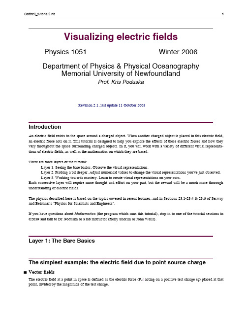
Visualizing electric fieldsPhysics 1051 Winter 2006 Department of Physics & Physical OceanographyMemorial University of NewfoundlandProf. Kris PoduskaRevision 2.1, last update 11 October 2005IntroductionAn electric field exists in the space around a charged object. When another charged object is placed in this electric field,an electric force acts on it. This tutorial is designed to help you explore the effects of these electric forces and how theyvary throughout the space surrounding charged objects. In it, you will work with a variety of different visual representa-tions of electric fields, as well as the mathematics on which they are based.There are three layers of the tutorial:Layer 1. Seeing the bare basics. Observe the visual representations.Layer 2. Probing a bit deeper. Adjust numerical values to change the visual representations you've just observed.Layer 3. Working towards mastery. Learn to create visual representations on your own.Each successive layer will require more thought and effort on your part, but the reward will be a much more thorough understanding of electric fields.The physics described here is based on the topics covered in recent lectures, and in Sections 23.1-23.4 & 23.6 of Serwayand Beichner's "Physics for Scientists and Engineers".If you have questions about Mathematica (the program which runs this tutorial), stop in to one of the tutorial sessions inC2039 and talk to Dr. Poduska or a lab instructor (Kelly Shorlin or John Wells).Layer 1: The Bare BasicsThe simplest example: the electric field due to point source charge‡Vector fieldsThe electric field at a point in space is defined as the electric force (F e L acting on a positive test charge (q) placed at thatpoint, divided by the magnitude of the test charge.(1)E ”=F ”e ÅÅÅÅÅÅÅq One way to picture the electric field due to a point source charge is with a vector field:The vector field shown above is a three-dimensional representation of the electric field originating from a point source charge at the center of the cube. Each arrow in the vector field shows the magnitude and direction of the electric force that would act on a positive test charge positioned at its tail. In this example, you can see that all arrows are pointing away from the point source charge (meaning that the source charge is a positively charged object). It's also true -- but a bit harder to see -- that the arrows that start closer to the source charge are much longer than those that start further away (meaning that the magnitude of the electric field -- and hence the magnitude of the electric force that would act on another charged object at that point in space -- is much larger close to the source charge).This picture of an electric vector field is consistent with the mathematical expression for the electric field due to a point source charge that we've seen in class:(2)E ”=k q ÅÅÅÅÅÅÅr 2 r `In this equation, E represents the electric field, k is Coulomb's constant, q is the magnitude of the source charge that generates the field, and r is the radial distance from the point charge. Remember that electric field is a vector quantity; r `means that the electric field of a point source charge is always directed radially inward or outward.Although an electric field is a three-dimensional (3D) entity, at a practical level, it is easier to look at the electric vector field in a two-dimensional (2D) slice that contains the source charge.Each arrow in the vector field shows the magnitude and direction of the electric force that would act on a positive test charge positioned at its tail. In this two-dimensional represenation, it is much easier to see that all arrows are pointing away from the point source charge (meaning that the source charge is a positively charged object), and that the arrows that start closer to the source charge are much longer than those that start further away (meaning that the magnitude of the electric field -- and hence the magnitude of the electric force that would act on another charged object at that point in space -- is much larger close to the source charge).The vector field shown above is a two-dimensional representation of the electric field, and it shows only those points that lie in a plane that contains the source charge. It doesn't matter which plane we pick, as long as it contains the source charge; Equation 2 assures us that the electric field only depends on the radial distance, in any direction away from the source charge.This discussion of dimensions brings up another possible way to picture the electric field around a point source charge. Since the magnitude of the electric field changes with the radial distance r from the source charge, we can also represent this change throughout space with a one-dimensional plot.Just as the vector field showed us that the magnitude of the electric field (i.e. the length of the vector) is much larger closer to the source charge than further away, so too does this plot of electric field versus radial distance.One thing that's easy to see with this plot of electric field versus distance is precisely how quickly the magnitude of the electric field decreases as the distance from the source charge increases. At a radius of 0.2 on the plot above, the magni-tude of the electric field is 20; at a radius of 0.4, the magnitude of the electric field has decreased to 5. This agrees with the mathematical expression above (Equation 1), which tells us that if we move twice as far from the source charge, the magnitude of the electric field is only one fourth as large (that's a decrease of 75%).‡Electric field linesThe vector field we've just seen is only one way to describe how the electric field varies throughout space. Another way of visualizing electric field patterns is to draw lines that follow the same direction as the electric field vector.How can one determine the magnitude and direction of the electric field at any one point in space from a plot of electric field lines? Here are the two key points to remember. First, the electric field direction at any one point in space is given by the direction tangent to the electric field line at that point. Second, the closer together the lines are in a given region of space, the larger the magnitude of the electric field in that region.In this case, you can see that all lines are directed away from the point source charge (meaning that the source charge is a positively charged object), and that the lines are more densely arranged closer to the source charge than those further away (meaning that the magnitude of the electric field -- and hence the magnitude of the electric force that would act on another charged object at that point in space -- is much larger close to the source charge).‡Lines of constant electric field magnitudeThere is yet another kind of plot which is useful for depicting how an electric field varies throughout space: a contour plot. This kind of representation is like a topographical map which shows lines of constant altitude; in this case, the lines correspond to lines of constant electric field magnitude.In this case, you can see that all lines of constant electric field magnitude are circles centred on the point source charge (meaning that the magnitude of the electric field depends on the radial distance from the source charge), and that the lines are more densely spaced closer to the source charge than those further away (meaning that the magnitude of the electric field -- and hence the magnitude of the electric force that would act on another charged object at that point in space -- increases rapidly close to the source charge).Two things about the electric field are difficult to see from this plot. First, is the source charge is a positively charged or negatively charged object? The only way to tell is to look at the labels on the contour lines to see whether they are positive electric fields (indicating a positive source charge) or if the electric fields are negative (indicating a negative point source charge). Second, the plot itself doesn't show us the direction of the electric field directly. However, we can reason through the direction without much trouble. We saw in the vector field and field line plots that the electric field is always directed radially inward or outward from the point source charge. This means that the electric field lines and vectors are always perpendicular to the lines of constant electric field magnitude, pointing radially inward (negative source charge) or outward (positive source charge).Why go to the trouble of a contour plot if electric field lines or vector fields are easier to decode? I show this kind of plot to you now because you'll soon see it again when we talk about electric potential, and we will be relating it back to the other kinds of plots you've seen in this tutorial. For now, though, we'll spend the rest of this tutorial with vector fields and field lines.Electric fields due to multiple point source chargesNow that we've seen a few different ways to visualize electric fields, let's apply these representations to electric fields that result from a collection of two or more point source charges.In class, we've seen that at any point in space, the total electric field due to a collection of point source charges is equal to the vector sum of the electric fields of the individual charges. In other words, we can use Equation 1 to determine the electric field due to the each of the point source charges individually, and then just add the results together to get the total electric field. Remember that the electric field due to a single point source charge is still a vector quantity, and that's why we have to make sure that we use vectors throughout to keep track of direction, as well as magnitude of the electric field at each point in space. We can write the vector sum in a compact format(3)E =k ‚i q i ÅÅÅÅÅÅÅÅÅÅr i 2r `Let's look at the electric vector field for two point source charges with the same magnitude of charge and the same sign.There are a few features of this plot worth mentioning. First, notice that the electric field vectors are no longer the same length for the same radial distance around one of the source charges. For example, the electric field is larger in the region directly between the two source charges than it is on the far sides of each source charge.Compare this electric vector field with electric field lines:Within a given region of space, the more closely spaced the lines, the greater the magnitude of the electric field. What happens if the charges have the same magnitude, but opposite signs?In this representation, the vectors point away from the positive source charge and towards the negative source charge, consistent with what we've seen with electric vector fields for single point source charges. Also, notice that electric field lines always originate from positive source charges and terminate at negative source charges.Just one more example, a bit more complicated this time: two point source charges, with different magnitudes and opposite charges. This time, we'll just look at the electric field lines.The same features apply, but now notice that the number of lines that begin (or end) at a given source is proportional to the relative magnitude of that particular source charge.Moving to three or more point source charges isn't any more difficult. The total electric field at any point in space is still just the vector sum of the electric fields due to each point source charge, and the electric field can still be represented in terms of vector fields or electric field lines.Layer 2: Probing a bit deeperA simple example: the electric field due to point source charge‡Changing the sign of the source chargeA point source charge produces an electric field that is directed radially inward or outward from the source charge, and its magnitude depends on the distance from the source charge (r ) and the magnitude of the source charge itself (q ).Here's an equation we saw earlier:(4)E ”=k q ÅÅÅÅÅÅÅr 2 r `How does the appearance of the vector field change we change the sign of the source charge? Try it yourself! The input cell below provides a way to change the value of q. Start by clicking on the input box, set q = -1 on the first line, and then press "Enter" (not "return") to see the affect this has on the vector field. (Note: The commands in the rest of the input box set up the equation and plotting parameters. You can see the value of q that you set will be used in an expres-sion very similar to Equation 4. You won't need to change anything other than the value of q during this part of the tutorial. However, if you're curious and would like to know more, talk to one of your lab instructors.)Cottrell_tutorial5.nb11 does the appearance of the vector field change we change the sign of the source charge? Try it yourself! The inputcell below provides a way to change the value of q. Start by clicking on the input box, set q = -1 on the first line, and then press "Enter" (not "return") to see the affect this has on the vector field. (Note: The commands in the rest of the input box set up the equation and plotting parameters. You can see the value of q that you set will be used in an expres-sion very similar to Equation 4. You won't need to change anything other than the value of q during this part of thetutorial. However, if you're curious and would like to know more, talk to one of your lab instructors.)our example above, you see that the arrows nearest the source charge cross each other when you set q = -1. This looks a bit funny, but there's no problem with our simulation. As we saw before, each arrow in the vector field shows the magnitude and direction of the electric force that would act on a positive test charge positioned at its tail. Arrows that start closer to the source charge are longer relative those that start further away, in direct proportion to the magnitude of the electric field. We could change our picture to avoid these arrows crossing each other by choosing to make all of theFor our example above, you see that the arrows nearest the source charge cross each other when you set q = -1. This looks a bit funny, but there's no problem with our simulation. As we saw before, each arrow in the vector field shows the magnitude and direction of the electric force that would act on a positive test charge positioned at its tail. Arrows that start closer to the source charge are longer relative those that start further away, in direct proportion to the magnitude of the electric field. We could change our picture to avoid these arrows crossing each other by choosing to make all of the arrow proportionally shorter, but it wouldn't change the actual magnitude of the electric field at any particular point.We've also seen that the magnitude of the electric field changes with the radial distance r from the source charge, so we can also represent this change throughout space with a one-dimensional plot. How does the appearance of the vector field change we change the sign of the source charge? Try it yourself! The input cell below provides a way to change the value of q. Start by clicking on the input box, set q = -1, and then press "Enter" (not "return") to see the affect this has on the electric field as a function of radial distance.By changing to a negative source charge, you see that the electric field has a negative value, just as Equation 4 says it should. You can also try changing the magnitude of the source charge (for example, let q = -2). What happens to the shape of the curve? What happens to the values of the electric field? These observations are also consistent with Equa-tion 4. If you don't understand why, seek out help from one of the lab instructors before proceeding.Electric fields due to multiple point source chargesRecall that the total electric field due to a collection of point source charges is equal to the vector sum of the electric fields of the individual charges. Remember that the electric field due to a single point source charge is still a vector quantity, and that's why we have to make sure that we use vectors throughout to keep track of direction, as well as magnitude of the electric field at each point in space.(5)E =k ‚i q i ÅÅÅÅÅÅÅÅÅÅr i 2r `Let's look at the electric vector field for three point source charges each with different charge magnitudes and signs. Try it yourself! The input cell below provides a way to change the value of q. Start by clicking on the input box, set q1 = 1,q2 = 2, and q3 = -1, then press "Enter" (not "return") to see the affect this has on the vector field.the vectors point away from positive source charges and towards the negative source charges, it is relatively easy to determine which of the three charges are positive. Since the length of the vectors is proportional to the magnitude of the total electric field at that point, in this example it is also easy to tell which charges are largest and smallest. Now, try putting in other combinations of charge magnitudes and signs in the input cell above to see if you can repro-duce the figure below.Because the vectors point away from positive source charges and towards the negative source charges, it is relatively easy to determine which of the three charges are positive. Since the length of the vectors is proportional to the magnitude of the total electric field at that point, in this example it is also easy to tell which charges are largest and smallest. Now, try putting in other combinations of charge magnitudes and signs in the input cell above to see if you can repro-duce the figure below.If you have difficulties with this exercise, talk to one of the lab instructors before proceeding.Layer 3: Working towards masteryYou've seen how electric vector fields change with the magnitude and signs of the source charges. Now you'll have the opportunity to change the positions of the source charges as well. The input cell below provides a way to change the values of charges (q1, q2, q3) and positions ({x1,y1}, {x2,y2}, {x3,y3}). Start by clicking on the input box to set the position of source charge 1 to be (x1 = 0.15, y1 = 0), source charge 2 at (0,0) and source charge 3 at (0,-0.15) and then press "Enter" (not "return") to see the affect this has on the vector field.Now, try putting in other combinations of charge magnitudes, signs, and positions in the input cell above to see if you can reproduce the figure below...and one more to try:Finally, we'll extend these explorations to electric field lines. We've saved these for last because the commands that we need to draw field lines with Mathematica are quite complicated. Don't panic! You won't need to learn (or enter) these commands yourself; as before, you will just adjust the magnitudes and signs of the source charges. To make things even simpler, most of the gory details are hidden from view. (If you'd like to see them, ask a lab instructor to show you how to "open" the cells below.)Here are a series of exercises for you to try. If you have questions, please ask a lab instructor for assistance.(1) Let q1 and q2 be positive, but change their relative magnitudes. What happens to the number of electric field lines around each source charge?(2) Compare the electric fields lines corresponding to the situation q1 = q2 = 1 with the electric field lines for q1 = q2 = 4. What happens to the number of electric field lines around each source charge? What does this tell you about how Mathematica is calculating the number of electric field lines to use?(3) Now let q1 = -1 and let q2 = 1. What happens to the number of electric field lines around each source charge? How are the shapes of the field lines different than when q1 = q2 = 1?(4) Finally, let q1 be any negative number, and let q2 be any positive number such that |q2| > |q1|. What happens to the number of electric field lines around each source charge? How are the shapes of the field lines affected?Here's one final exercise to try: if q1 = -4, what value must q2 have to yield the electric field lines below? (Check your answer by using the input cell above!)End of Tutorial。

TCL Tutorial基本语法指令

TCL Tutorial 基本語法與指令Original written by Rick In 2003Revision by maa In 2004/6目錄一、TCL 簡介 (3)二、TCL 語法 (4)三、資料型態 (9)String 字串資料態 (9)List 串列資料型態 (17)Array 陣列資料型態 (20)四、控制結構 (22)If Then Else (23)Switch (24)While (26)For (27)Foreach (28)Break 與Continue (29)Catch (29)五、Procedure (30)六、TCL 內建指令 (32)TCL的全名為Tool Command Language，唸作”Tickle”，事實上它是一個Scripting Language（俗稱劇本語言或腳本語言），也是一個直譯器(Interpreter)。

TCL 語言有三個特色：1. 語法簡單，容易上手2. TCL 的身份如同UNIX裡的Shell languages像是Bourne Shell (sh)、CShell (csh)、Korn Shell (ksh) 與 Perl一樣，用來執行與控制系統上的程式。

TCL具備足夠的程式化能力 (variable、flow control、procedure) 與存取檔案、程序 (Process) 及網路的功能，供組裝既有軟體元件以建立符合需求的新工具。

3. 可內嵌 (embed) 到應用程式中，讓軟體使用者透過程式員提供的高階 TCL指令，自訂應用程式的行為。

除了上列三個主要特色外，底下所列的幾點也是 TCL 語言成功的原因：跨平台，可在各種系統 (UNIX、Windows、Macintosh 等) 執行 TCL 程式強大的字串處理能力『常規表示式 (Regular Expressions)』，協助程式員使用表示式的規則或樣式 (pattern)，用來搜尋、比對、粹取或是取代符合樣式的複雜字串。

Volocity Tracking Tutorial说明书

DataLive Cell TrackingWorkflowTracking objects may be appropriate if you are interested in characterizing the movement of objects (i.e. their speed, direction), or monitoring properties of objects as they move over time. In Volocity, tracking is a two stage process:1) The identification of the objects.2) The analysis of the positions of those objects and the building of tracks.Finding objectsClick once on the data in the library list and click on the Measurements tab to display the Measurement View. The image is shown in the mode that best shows the objects to be measured, and below it is an area where all measurements made will be displayed. At the top left of the screen is an area where a measurement protocol will be built, to find objects of interest in the dataset and track them, using the list of tasks in the area below.Volocity Tutorial TrackingThis tutorial will demonstrate how to perform tracking using Volocity ®.TUTORIAL NOTEIt is important that the Measurement Protocol identifies objects as accurately as possible in each timepoint as this will be essential for the tracking algorithm.The objects within this dataset do not exhibit the same intensity values throughout the time-course; therefore thresholding on the same intensity values in each timepoint is unlikely to be successful. The task “Find Objects Using SD Intensity” selects intensities within a specified number of standard deviations from the mean. Select this task and drag and drop it into the measurement protocol.Where intensities are found within range a colored overlay is applied. Groups of selected intensities form objects. View the image, with object overlays, in different ways by changing the mode of view in the top left.In this example, some of the objects formed are too large, they are actually two or more objects currently identified as one. Use the task “Separate Touching Objects” to improve this situ ation. The Object size guide, shown in the “Separate Touching Objects” task box, can be set to the approximate size of the smallest object that can be created by the separating step. In this example the Object size guide is 0 µm3, the best separation is achieved by not restricting the size of objects that will be made.TrackingOnce objects have been identified they can be connected together by tracks. Drag and drop a “Track Objects” task to the measurement protocol.The tracking algorithm uses the centroid measurement for each previously identified object to determine whether there is any movement of objects over time. Tracks are generated by connecting the centroids so as to trace the path of a moving object. The track objects task will always place itself at the bottom of the list of tasks in the protocol since objects must be found before they can be tracked.To see the results of the “Track Objects” task all timepoints must be measured. Select Measure all timepoints from the Measurements menu.To alter how the tracks are measured, click on the cog icon on the “Track Objects”task to access the secondary dialog for this task.For example, it may be necessary to set a maximum distance between objects, in this example 5 µm.Every object measured is given a unique object ID. Objects that have been tracked, and are therefore determined to be the same object in different locations are given the same Track ID; however their object ID remains the same.In the drop-down menu at the top of the measurements table, filter by tracks to just see measurements made on tracks. This contains summary information such as track length, the average velocity for the duration of the track, the trajectory and the meandering index.Filter by objects and sort by Track ID to see individual properties of the object and how they change over time.Now that the objects have been measured and tracked, we should confirm these tracking results by examining individual tracks. Select a row (shift-click to select multiple rows) in the table, representing a track, to show the individual overlay of that track on the image..Showing object feedback for the current timepoint only can assist in understanding what is being shown. To adjust the feedback that is displayed on the image, select Feedback Options... from the Measurements menu.Use the time navigation controls to compare the feedback with the underlying image data.The most likely problem with tracks is caused by setting the wrong maximum distance between objects in the secondary dialogue of the “Track Objects” task (as discussed previously). If tracks are incorrect because they switch to different objects part way through the time series, the maximum distance assigned is too great. If tracks are incorrect because they do not follow an object far enough in the time course, the maximum distance may be too small. Adjust as appropriate.Analysis of tracking dataThe tracking process generates information about object movement and object properties over time. Tracksrecord information about the behavior of the object for the duration of the time that it was followed. Individualproperties for each object, some of which are added by the tracking step, are also recorded.To easily extract what is of particular interest from this wealth of information, you may store all the measurements, in table format, as a separate Measurement Item within the library, and then perform further analysis. Select Make Measurement Item… from the Measurements menu, remembering to select Measure All Timepoints when prompted.Raw tables, analysis tables and charts, created within the resulting Measurement Item, can all be viewed in Volocity or exported as text or image files.is a registered trademark of PerkinElmer, Inc. All other trademarks are the property of their respective owners.。

wincoot简易教程

Tutorial 使用指南

使用指南（Tutorial）修订版序从首次接触这个软件到现在，有一段时间了。

那时由于急着使用，因此对一些认为不太重要的地方没有进行整理。

后来才发现，其实每一部分都是很有用的。

此修订，一个是将LineSim（Tutorial）与后加的Crosstalk（Tutorial）的目录统一起来，再有就是原文基础上增加了多板仿真（Tutorial）一节。

同样，对于那一时期我整理的BoardSim 、LineSim使用手册，也有同样的一个没有对一些章节进行翻译整理问题（当初认为不太重要）。

而实际上使用时，有一些东西是非常重要的，同时也顺便进行了翻译。

此外，通过使用，对该软件有了更多一些理解，显然以前只从字面翻译的东西不太好理解，等我有时间将它们重新整理后，再提供给初学的朋友。

对在学习中给予我大量无私帮助的Aming、pandajohn、lzd 等网友表示忠心的感谢。

P o q i0552002-8-202002-8-20目录使用指南（TUTORIAL ） 1 第一章 LINESIM4 1.1 在L INE S IM 里时钟信号仿真的教学演示 4 第二章时钟网络的EMC 分析 7 2.1 对是中网络进行EMC 分析7 第三章 LINESIM'S 的干扰、差分信号以及强制约束特性 8 3.1 “受害者”和 “入侵者” 8 3.2如何定线间耦合。

8 3.3 运行仿真观察交出干扰现象9 3.4 增加线间距离减少交叉干扰（从8 MILS 到 12 MILS ） 93.5 减少绝缘层介电常数减少交叉干扰 93.6 使用差分线的例子（关于差分阻抗） 93.7仿真差分线 10第四章 BOARDSIM114.1 快速分析整板的信号完整性和EMC 问题 11 4.2 检查报告文件 11 4.3 对于时钟网络详细的仿真 11 4.4 运行详细仿真步骤： 11 4.5 时钟网络CLK 的完整性仿真 12 第五章关于集成电路的MODELS 145.1 模型M ODELS 以及如何利用T ERMINATOR W IZARD 自动创建终接负载的方法 14 5.2 修改U3的模型设置（在EASY.MOD 库里CMOS,5V,FAST ） 14 5.3 选择模型（管脚道管脚）C HOOSING M ODELS I NTERACTIVELY （交互）, P IN -BY -P IN 14 5.4 搜寻模型（F INDING M ODELS (THE "M ODEL F INDER "S PREADSHEET ) 15 5.5 例子：一个没有终接的网络 15 第六章 BOARDSIM 的干扰仿真 186.1 B OARD S IM 干扰仿真如何工作 186.3仿真的例子：在一个时钟网络上预测干扰 18 6.3.1加载本例的例题“DEMO2.HYP” 18 6.3.2A UTOMATICALLY F INDING "A GGRESSOR"N ETS 18 6.3.3为仿真设置IC模型 19 6.3.4查看在耦合区域里干扰实在什么地方产生的 19 6.3.5驱动IC压摆率影响干扰和攻击网络 20 6.3.6电气门限对比几何门限 20 6.3.7用交互式仿真"CLK2"网络 20 6.4快速仿真:对整个PCB板作出干扰强度报告 20 6.5运行详细的批模式干扰仿真 21第七章关于多板仿真237.1多板仿真例题，检查交叉在两块板子上网络的信号质量 23 7.2浏览在多板向导中查看建立多板项目的方法 24 7.3仿真一个网络A024 7.4用EBD模型仿真24HyperLynxHyperLynx是高速仿真工具，包括信号完整性（signal-integrity）、交叉干扰（crosstalk）、电磁屏蔽仿真（EMC）。

tutorial 中文手册2.2

感谢本tutorial Manual 2.2翻译文档在许多网友的关心和支持下，得以翻译成功，在此对他们表示热烈地感谢：蝈蝈、fiona、kailinziv、Yan、杀毒软件、tiny0o0、timothy、prolee等关心TG手册翻译的热心朋友。

关于本文档内容说明：由于本手册由不同网友翻译，可能对某些概念有不同的理解，翻译可能不大一样，但决不影响理解，欢迎大家探讨。

再一次对各位网友的努力和汗水表示感谢！如有什么问题可以联系我：Mail:tiny0o0@注：本文档内容版权归X Y Z scientific company 所有，谢绝任何意图商用。

Ｉ、TrueGrid介绍True Grid是一套优秀的、功能强大的通用网格生成前处理软件。

它可以方便快速生成优化的、高质量的、多块结构的六面体网格模型。

作为一套简单易用，交互式、批处理前处理器，True Grid支持三十多款当今主流的分析软件。

True Grid是基于多块体结构（multiple-block-structured）的网格划分工具，尽管这个指南手册开始会提供一些介绍信息，新手还是强烈要求阅读用户手册（True Grid® User’s Manual）的前２章，用户指南和参考手册。

True Grid是几何和网格形成过程是分开进行。

曲面和曲线形成的方式有以下几种：内部产生，从CAD/CAE系统导出IGES格式导入ＴＧ，或用vpsd命令导入多边曲面。

块网格（block mesh）初始化然后通过各种变换与几何模型匹配形成最后的有限元模型。

True Grid网格划分过程：运用block命令初始化块网格；块网格部分会被删掉以使拓扑结构与划分目标对应；块网格部分通过移动，曲线定位，曲面投影等方法进行变换；网格插值、光滑和Zoning(控制边界节点分布)等技术可以用来形成更好的网格；块网格之间独立形成，然后通过块边界面（ＢＢ）和普通节点合并命令（指定容差范围内合并）将各块网格合并成完整的有限元模型。

tutorial-2

Coot Tutorial II:More Advanced UsageCCP4School APS2009February10,2010The idea here is to use more advanced1tools of Coot.There will be less de-scription of low-level widget manipulation in this tutorial-we presume that you already have experience with that.You may well trip over issues not discussed here2.1PreambleWhen automatic building fails,typically because the resolution limit of your data is too low,then building the molecule“by hand”may be the only way to proceed. Recognizing the shape of main-chain and side-chain densities is valuable and this tutorial aims to introduce these to you.Note that this tutorial map is an easy map to build into,the sidechains are(mostly)clear.If you want a more realistic“bad”map,you can apply a resolution limit to the data read in from the MTZﬁle3.Using just a map and a sequence,we will attempt to generate a model.This model can then be validated and reﬁned with Refmac for several rounds.With some experience you should be able to get an R-factor of less than20%in less than 30minutes.2Skeletonization and Baton BuildingYou can calculate the map skeleton in Coot directly:Calculate→Map Skeleton...→On.This can be used to“baton build”a map.You can turn off the coordinates and try it if you like(the Baton Building window can be found by clicking“Ca Baton Mode...”in the Other Modelling Tools dialog.I suggest you use Go To Atom and start residue2A.This allows you to build the complete A chain in the correct direction and you can directly compare it to the real structure afterward4.Once you are at residue2A,use the Display Manager to turn off the‘‘tutorial-modern.pdb’’and don’t look at it again until you have ﬁnished building,validating and reﬁning.Remember,when you start,you are placing a CA at the baton tip and at the start you are placing atom CA1.This might seem that you are“double-backing”on yourself-which can be confusing theﬁrst time.So build from the N-terminus to the C(it takes about15minutes or so).There are96residues to build.1“less commonly-used”might be a better description2Feel free to shout out if you do,several others may have this same problem and we can examine the issue together.3the resolution limit widget will appear when you activate the“Expert Mode“button.4if don’t follow this instruction,you could well build a symmetry related molecule,which is per-fectly valid,of course,just that the comparison versus the correct structure will be more difﬁcult.Note that you need at least6CA baton points for CA Zone to Mainchain to work53Key BindingsIf you look at”Paul’s Key Bindings”6in the Coot Wiki7,you will see a page of customizations.One of those customizations can help you in Baton-Building mode -and that is the“quoteleft”key binding.So,cut the bindings out of the web page,paste them into aﬁle and then use Calculate→Run Script...to evaluate thatﬁle8.To check that your key-bindings are activated,Use Extensions→Key Bindings....Now,we can use quoteleft(or“backquote”,”‘”is how it might appear on the keyboard)to accept the baton position-this is much more convenient than using the“Accept”button9.4At the end of the ChainAt some stage10you will come to a point where no progress can be made,the only direction takes us into density we’ve already built into.OK,so stop:Dismiss.Now we need to turn these CA positions into mainchain.Calculate→Other Modelling T ools→CA Zone to e the Go T o Atom dialog to centre on theﬁrst residue of“Baton Atoms”,click it,then centre on the last residue of“Baton Atoms”and click on that.[Coot thinks for a several seconds while building a mainchain]OK,great,we have a mainchain.Let’s tidy it up:Extensions→Stepped Reﬁne.Reﬁne the“mainchain”molecule,watch it as it goes.Is it making mistakes?That reﬁnement may have gone to quickly to make a note of problem areas,so use Validation→Density Fit Analysis on the“mainchain”molecule andﬁnd areas that are marked with large spikes.“There are none”you say?Good11.Let’s move on.5Assign SequenceLet’s tell Coot that we have a sequence associated with this set of CA points.So, Extensions→Dock Sequence→Assign SequenceTurn on auto-ﬁt of residuesSo when theﬁle is assigned“Assign Closest fragment”.[Coot thinks for a several seconds while assigning sidechains,then goes about mutating andﬁtting the residues]What’s that you say?Coot didn’t do that?Well,that’s because you mainchain model is too bad for Coot to recognize the sidechain positions.You need to review you mainchain model and make sure sure that the CBs are in density and pointing 5otherwise it silently fails-more feedback will be added in later versions.6Use Bernhard’s Key-bindings if you are using pythonized or WinCoot7you canﬁnd a link to this from the Coot web page8“read it in”,you might say9You can do that as well,of course,but clicky-clicky pressy button is for Coot noobs,and that’s not us, right?10hopefully residue9611If that’s not what you say,you can use the reﬁnement or other tools that we learned about in the ﬁrst tutorial to improve theﬁt to density.in the right direction.When you have improved you model sufﬁciently well,Coot will apply the sequence to it using the above method.Change the Chain ID from““to“A”.6Cell and SymmetryDisplay Symmetry Atoms:Draw→Cell&Symmetry→Master Switch:Show Symmetry Atoms→Y es and OK.By zooming out and eyeballing the density,check for unassigned density.[Coot displays symmetry-related atoms in grey-by default(you may not see many symmetry related atoms,it depends on where in the unit cell you are)]7Build another moleculeNow we need to build another molecule(the NCS related copy).So using the map skeleton search around toﬁnd a volume of density not already build(and not symmetry related to the model already built).Here’s a hint,ﬁnd the a helix in the skeleton.•Using the Other Modelling Tools,place a helix over the skeleton points of the skeleton.•Improve theﬁt of the skeleton,taking note that the N and C terminus of the helix are well-ﬁtted.•Associate the same sequence with the new Helix molecule•Dock sidechains on the new molecule(it should work if your helix is good)•Now compare the Helix molecule with the previously built model.Find matching start and end point on the helix and previous model.•LSQﬁt a copy of the previous model on top of the Helix molecule [Coot displayes a new molecule that almostﬁts the so-far unbuilt density.] Let’s call this new chain,chain“B”•Now clean up theﬁt,ﬁrst do a rigid body reﬁnement of the whole new model...•then an All Molecule stepped reﬁne should make theﬁt nice.8Merge MoleculesMerge the“B”chain into the“A”chain molecule above:Calculate→Merge molecules→Append/Insert Molecule(s)[Choose the most recent mainchain molecule]into Molecule[Choose the molecule of the A chain]→Merge.9GhostsUnfortunately,there is no slick way to make Coot rebuild ghosts for this composite molecule.We need to write out the pdbﬁle and read it in again-inelegant.File→Save Coordinates,[Choose the molecule that does now contains both the A and B chains]→Select Filename...Pick aﬁlename then use File→Open Coordinates...to read it in again.Check the console as you do this,Coot will tell you that there are NCS related molecules.If12it does this,we’re in business.In the following,you will need to know theﬁrst and last residue numbers in the“A”e the Go To Atom dialog toﬁnd them.If ghosts appear,use:Extensions→NCS...→Copy NCS Residue ing“A”13as the Mas-ter Chain ID thenﬁll in theﬁrst and last residue numbers of the A chain.[Coot builds the B chain as an NCS copy of the A chain]10Rinse,RepeatUse NCS jumping(the’O’key)to see NCS differences.Now unmodelled blobs-like we did before.Find the ligand(3GP),merge it in.Reﬁne using Refmac.Validate.Rebuild.11Make some pictures•Highlight active site,with ligand.Take a screenshot.•Use Raster3D to take a screenshot•Now make a Raster3D image without spheres for atoms,how do you do that?•Now give the ligand a dotted surface•Now Use Extension→Mask Map to make a map that has density only around the ligand.•Now take the residues in the active site,use Copy Fragment and merge molecule to make a single mlecule of them.Display this atom selection as an electrostatic surface12ViewsTry out the“View”system•Zoom out to see the whole molecule on the screen•Recentre and Zoom in to the active site•Play Views...12When13presumably13More ExercisesWhat does“Another Level”do?What does“Multi-chicken”do?Use the skeletonization of a map toﬁnd a e Calculate→Other Modelling T ools to add a helix there.Try to represent the map with a higher resolution grid(use Edit→Map Parame-ters).Do you prefer that?Why?Use the EDS service to download1H4P.Can youﬁnd anything wrong with the main-chain?If so,how can you correct it?。

课课家教育-Python入门到精通系列(入门篇)视频教程

课程目标：通过本套课程的学习，让我们每个人都可以轻松的遨游在Python世界里，把复杂的语言简单化，满足企业运维日常的数据分析和运维系统的管理，编写自动化运维平台，让我们的运维更加的高大上！是大家升职加薪必备课程。

通过本次课程的学习，大家可以跟着时代的步伐，去展示自己的技能，高薪就业。

适合对象：本套课程适合有Linux Shell编程基础，想进一步提升自己在企业运维更好的运维的人员，有自动化运维意识的同学，期待跟大家相识在pyt hon编程的世界里。

学习条件：需要专注去学习，愿意付出时间去改变自己，成就自己！学习宣言：本套课程还是以企业实战为主，理论为辅，让大家快速上手去操作，能快速写出高大上的运维管理系统。

相信每个人付出一定收获满满！目录第1节Python编程入门安装第2节Python变量及常用算法00:26:33第3节Python编程条件语句学习00:21:19第4节Python编程函数及模块实战00:30:18第5节Python编程数据结构-列表00:27:13第6节Python元组及字典案例讲解00:22:32第7节Python阶段综合实战脚本编写00:44:52第8节Python字典查询系统编写00:31:01第9节Python编程异常错误处理00:18:09第10节Python面向对象编程入门简介00:24:13第11节Python面向对象编程二00:23:26第12节Python面向对象编程类及学习心得00:10:30第13节Python编程标准库学习00:23:37课程网址：/course-3938.html?A=wenku。

tutorial节选

Things to Know Before Getting Started with eQUEST Whole building analysis. eQUEST is designed to provide whole Building performance analysis to buildings professionals, i.e., owners, designers, operators, utility & regulatory personnel, and educators. Whole building analysis recognizes that a building is a system of systems and that energy responsive design is a creative process of integrating the performance of interacting systems, e.g., envelope, fenestration, lighting, HVAC, and DHW.在开始之前需要知道的事情与eQUEST关于整个建筑的分析。

eQUEST旨在提供整个建筑性能分析建筑专业人士,即所有者,设计师、运营商、实用工具和监管人员,和教育家。

从整个建筑分析认识到建筑是一个系统的系统和能量响应设计是一种创造性的整合过程性能交互的系统,例如,维护结构、开窗、照明、空调和DHW。

Therefore, any analysis of the performance consequences of these building systems must consider the inter actions between them … in a manner that is both compre hensive and affordable (i.e., model preparation time, simulation runtime, results trouble shooting time, and results reporting).因此,任何分析的性能影响这些建筑系统必须考虑…它们之间的交互的方式,既全面和负担得起的(例如,模型的准备时间,模拟运行时间,结果故障排除时间,和结果报告)。

Autolab control tutorial

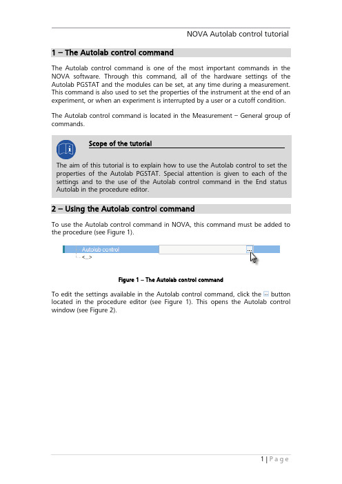
1– The Autolab control commandThe Autolab control command is one of the most important commands in the NOVA software. Through this command, all of the hardware settings of the Autolab PGSTAT and the modules can be set, at any time during a measurement. This command is also used to set the properties of the instrument at the end of an experiment, or when an experiment is interrupted by a user or a cutoff condition. The Autolab control command is located in the Measurement – General group of commands.2– Using the Autolab control commandTo use the Autolab control command in NOVA, this command must be added to the procedure (see Figure 1).Figure 1 – The Autolab control commandTo edit the settings available in the Autolab control command, click the button located in the procedure editor (see Figure 1). This opens the Autolab control window (see Figure 2).Figure 2 – The Autolab control windowThree different default sections are located in the Autolab control window, on the left-hand side1:•PGSTAT302N2:this section is used to define all the settings of the main working electrode and the Autolab. The settings are displayed in two panels: Basic and Advanced.•DIO: this section is used to set the settings of the digital input/outputs of the Autolab3.•Summary:this section is used to display the summary of all the settings defined with the Autolab control command.Depending on the hardware setup, additional sections can be available in the Autolab control window. Figure 2 displays one additional section for the BAmodule.1 If other optional modules are selected in the Hardware setup, additional sections will be shown in the Autolab control window.2 The name of this section depends on the type of instrument specified in the hardware setup.3 More information on the use of the DIO can be found in the External devices tutorial.2.1– Invalid settingsWhen invalid settings are defined in the Autolab control command, for example using a procedure that includes settings incompatible with the instrument connected to the computer, the Autolab control window will automatically open on the summary section, highlighting the invalid settings in red (see Figure 3).Figure 3 – Invalid settings are displayed in the summary section, in redTo remove the invalid settings, click the setting as shown in Figure 3. It will be deleted from the Autolab control.3– Autolab PGSTAT settingsThe settings for the main Autolab potentiostat/galvanostat are defined in the first section of the Autolab control window. This section is identified by the name of the type of instrument specified in the hardware setup.The Autolab settings are specified in two different panels:•Basic: the most common settings of the instrument.•Advanced: special settings relevant for special applications.The Autolab control window always opens with the Basic section active.3.1– Basic settingsThe following basic settings can be specified using the Autolab control command: •Cell (On/Off): switches the Autolab PGSTAT cell switch on or off.•Mode (Potentiostatic/Galvanostatic): defines the mode of the PGSTAT.•Current range:defines the current range for Autolab PGSTAT. The available current ranges depend on the hardware setup. The optional ECD module extends the current range down to 100 pA and the Booster extends the current range up to 20 A (see Figure 4).Figure 4 – The available current ranges depend on the hardware setup• Bandwidth: defines the bandwidth of the Autolab PGSTAT: three settings are available: high stability, high speed and ultra-high speed 4.• iR Compensation (On/Off): switches the iR compensation circuit on or off 5.• iR Compensation value: defines the value of the compensated resistance used in the iR compensation circuit 5. The value range depends on the active current range.3.2 – Advanced settingsThe Advanced settings panel can be displayed by clicking the button in the Autolab control window (see Figure 5).Figure 5 – The Advanced settings panel of the Autolab control command4More information on the bandwidth settings of the Autolab PGSTAT can be found in the NOVA Getting started.5 Not available on the PGSTAT10 and the µAutolab II/III.The following advanced settings can be specified using the Autolab control command:•External input (On/Off): switches the external input of the PGSTAT on or off6.•Oscillation protection (On/Off): switches the oscillation protection circuit on or off6.•Reference voltage: defines the value of the reference voltage.•Offset.Value: defines the value of the offset DAC of the Autolab.•DAC164 1: defines the output voltage of the DAC164 module, BNC output #1.•External 1: defines the converted output voltage of the DAC164 module, BNC output #1 used to control the external device defined in the hardware setup.Depending on the hardware setup, additional settings can be defined in the Advanced panel (see Figure 6).Figure 6 – Additional module settings are available on the Advanced panel •FRA32M/FRA2 input (Enabled/Disabled): enables or disables the FRA32M or FRA2 module input on the summation point of the PGSTAT.•SCAN250/SCANGEN input (Enabled/Disabled): enables or disables the linear scan generator module (SCAN250 or SCANGEN) input on the summation point of the PGSTAT.6 Not available on the PGSTAT10, PGSTAT20, µAutolab II/III, PGSTAT101/M101 and PGSTAT204.4– µAutolab II/III settings4.1– Basic settingsWhen the µAutolab type II or III is used, the following basic settings are available (see Figure 7):Figure 7 – The basic settings for the µAutolab•Cell (On/Off): switches the µAutolab cell switch on or off.•Mode (Potentiostatic/Galvanostatic): defines the mode of the µAutolab.•Current range: defines the current range for µAutolab.•Bandwidth:defines the bandwidth of the µAutolab: two settings are available: high stability and high speed7.7 More information on the bandwidth settings of the µAutolab can be found in the NOVA Gettingstarted.4.2– Advanced settingsThe Advanced settings panel can be displayed by clicking the button in theAutolab control window (see Figure 8).Figure 8 – The advanced settings of the µAutolabThe following advanced settings can be specified using the Autolab control command:•Reference voltage: defines the value of the reference voltage.•Vout: defines the output voltage of the Vout BNC output located on the backplane of the µAutolab.•External 1: defines the converted output voltage of the Vout BNC output located on the backplane of the µAutolab used to control the external device defined in the hardware setup.5– PGSTAT101, PGSTAT204 or M101 settings5.1– Basic settingsWhen the PGSTAT101, PGSTAT204 or M101 is used, the following basic settings are available (see Figure 9):Figure 9 – The basic settings for the PGSTAT101 or M101•Cell (On/Off): switches the Autolab PGSTAT101/PGSTAT204/M101 cell switch on or off.•ode (Potentiostatic/Galvanostatic):defines the mode of the PGSTAT101, PGSTAT204 or M101.•Current range:defines the current range for Autolab PGSTAT101, PGSATT204 or M101.•Bandwidth:defines the bandwidth of the PGSTAT101, PGSTAT204 or M101: three settings are available: high stability, high speed and ultra-highspeed8.•iR Compensation (On/Off): switches the iR compensation circuit on or off.•iR Compensation value: defines the value of the compensated resistance used in the iR compensation circuit5. The value range depends on the activecurrent range.8M ore information on the bandwidth settings of the PGSTAT101 or M101 can be found in the NOVA Getting started.5.2– Advanced settingsThe Advanced settings panel can be displayed by clicking the button in theAutolab control window (see Figure 10).Figure 10 – The advanced settings for the PGSTAT101/M101•Reference voltage: defines the value of the reference voltage.•Offset.Value: defines the value of the offset DAC of the Autolab.•Internal dummy cell (On/Off): switches the internal dummy cell on or off.•ADC filters: specifies the status of the ADC filters (On/Off). When the filter is On, a low pass filter with a cutoff frequency of 22 kHz is applied on the input signals of the ADC.•Synchronization line: defines the status of the synchronization line9 used in M ulti Autolab measurements. Setting the bit ON enables hardware synchronization10.•Vout: defines the output voltage of the Vout BNC output located on the optional monitor cable11 of the PGSTAT101, PGSTAT204 or M101.•External 1: defines the converted output voltage of the Vout BNC output located on the optional monitor cable11 of the PGSTAT101, PGSTAT204 or M101 used to control the external device defined in the hardware setup.9 This is only functional in the M101 modules installed in the Multi Autolab cabinet.10M ore information on the use of the synchronization line can be found in the M ulti Autolab tutorial, available from the Help menu.11M ore information on the optional monitor cable for the PGSTAT101, PGSTAT204 or M101 module can be found in the Getting Started manual.6– Using the Autolab control commandThe settings available in the Autolab control can be defined during an electrochemical measurement by adding the Autolab control command in the procedure, whenever one of properties of the instruments needs to be changed.The Autolab cyclic voltammetry potentiostatic procedure provides a good example of the use of the Autolab control command at the beginning of the procedure (see Figure 11).Figure 11 – The Autolab Cyclic voltammetry potentiostatic procedureIn this procedure, the Autolab control command is used to specify the initial settings of the instrument. The following properties are defined in the command: •WE(1).Current range: 1 mA•WE(1).Bandwidth: High stability•WE(1).Mode: PotentiostaticThese settings are displayed in the procedure editor, below the Autolab control command (see Figure 12).Figure 12 – The settings defined in the Autolab control command are displayed in theprocedure editorChanging the settings in the Autolab control command can be done by clicking the button. The Autolab control window will appear, displaying the settingsdefined in the command. All settings that have button indicated on the right inthe Autolab control window are specifically defined in the Autolab control command (see Figure 13).Figure 13 – The settings specified in the Autolab control are identified by a button Changing the initial current range from 1 mA to 100 µA can be done using the dropdown list (see Figure 14).Figure 14 – Changing the current range can be done using the dropdown listClicking the button located next to the properties specified in the Autolabcontrol command changes the property to the current value of the instrument (see Figure 15).Figure 15 – Clicking the sets the property to the active value on the instrument (activecurrent range on the instrument: 1 µA)Click the OK button after the settings have been changed. The Autolab control command will be updated in the procedure editor (see Figure 16).Figure 16 – The modified Autolab Cyclic voltammetry procedure: the initial current range hasbeen reset to default (1 µA)Additional settings can be defined, using an existing Autolab control command located in the procedure editor or by adding additional Autolab control commands to the procedure.Keep in mind that the settings defined in the Autolab control command are all set when the procedure executes the command12.Figure 17 shows the Autolab cyclic voltammetry procedure with two additional settings defined in the Autolab control command:•iR Compensation: On•iR Compensation value: 100Figure 17 – The Autolab cyclic voltammetry potentiostatic procedure modified using the Autolab control command: the iR compensation circuit is switched on and the iRcompensation value is set to 100 OhmThe parameters of the Autolab control shown in the procedure editor can be linked to control commands like an Input box or a Repeat for each value command (see Figure 18).12The settings defined in the Autolab control are set sequentially in order to avoid possible hardware conflicts.Figure 18 – Using an input box in combination with the Autolab control command7– End status AutolabThe End status Autolab instruction is always present in the header of the procedure, alongside the title, the remarks field, the signal sampler, the options,instrument description and serial number field (see Figure 19).Figure 19 – The End status Autolab is located in the header of any procedureThe End status Autolab is a special Autolab control command which can be usedto define the settings of the Autolab whenever a measurement stops.This command is always the last executed command and it is triggered by the following events:•The measurement finishes normally:before the data is saved in the dasectionase, the End status Autolab command is executed, setting the final properties of the instrument.• A cutoff condition is encountered: if a cutoff condition designed to stop the complete procedure is triggered during the measurement, the procedure stops immediately, sets the instrument according to the End status Autolab command and stores the data in the dasectionase.•The user stops the measurement: if the user interrupts the measurement by pressing the stop button, the procedure is stopping as soon as possible, the instrument is set to the status defined in the End status Autolab command and the data is stored in the database.To edit the End status Autolab command, click the button located next to the command in the procedure editor (see Figure 20).Figure 20 – Using the End status Autolab control to set the Cell off at when themeasurement stops8– Extended voltage rangeThe voltage setting of the Autolab PGSTAT13 is defined by the sum of two DAC channels internally connected to the summation point of the control amplifier. One of the DAC is called the Scanning DAC and the other DAC is called the Offset DAC. Both DAC’s have a range of ± 5 V. The scanning DAC can be modifiedduring an electrochemical measurement, while the offset DAC can only be modified when the cell is switched off, to prevent interference with the ongoing measurement.In practice this means that the potential range of the Autolab will be ± 5 V with respect to the value of the offset DAC.The startup settings of the Autolab PGSTAT are the following:•Scanning DAC: 0 V•Offset DAC: 0 VUsing these initial settings, the Autolab PGSTAT is capable of applying any voltage value in the -5 V to 5 V range (with respect to the offset DAC value of 0 V). To apply a voltage outside of this potential range, the offset DAC value must be adjusted.For example, to apply 7 V on the cell during an electrochemical measurement, the following settings can be used14:•Scanning DAC: 2 V•Offset DAC: 5 VUsing these settings, the Autolab PGSTAT can be used to set the potential of the working electrode to any value between 5 V and 10 V during an electrochemical measurement.Using the Autolab display, it is possible to manually control the potential or current applied. The offset DAC will be automatically adjusted to the required value depending on the specified potential or current (see Figure 21).13 This does not apply for the µAutolab.14 Other combinations are possible.Figure 21 – The potential range depends on the value of the offset DAC (left – Offset value: 0V, right – Offset value: 5 V)During measurements, NOVA will also automatically adjust the offset DAC value is order to reach the required potential or current values. If the specified range for the scanning DAC is larger than 10 V (± 5 V) within a single measurement command, an error will be displayed during validation (see Figure 22).Figure 22 – An error is displayed when the specified value range is larger than 10 V for asingle commandNOVA can adjust the offset DAC during a measurement, if needed, in between different measurement commands. However, the offset DAC should not be modified when the cell is on during a measurement. A warning is provided during validation if the procedure requires the offset DAC to be reset during the experiment (see Figure 23).Figure 23 – A warning is provided when the offset DAC is reset while the cell is switched on If the cell is not switched off when the offset value is modified, the potential applied to the cell will not be properly controlled (as shown in Figure 24).Figure 24 – Detail of the potential profile of a potential adjustment from 0 to 8 V in two steps (the first step, starting at 0.01 s corresponds to the setting of the offset DAC, the second step, at 0.02 s corresponds to the setting of the scanning DAC)Figure 24 shows how the potential is adjusted, from 0 V to 8 V in the Autolab when both the offset DAC and the scanning DAC are modified in the procedure, with the cell switched on. The setting of the DACs has been intentionally delayed in this example to show the slower settling of the offset DAC compared to the scanning DAC.This slow response of the offset DAC, combined with the fact that the software is not able to set both DACs at the same time means that there will always be anuncontrolled potential profile between two consecutive potential values when the offset DAC needs to be adjusted. Consequently, an unexpected current response could be observed (see Figure 25).Figure 25 – Current response corresponding to the potential profile shown in Figure 24measured on dummy cell (c)This restriction only applies to measurement commands that require the offset DAC to be adjusted.It is therefore highly recommended to switch the cell off whenever the offset DAC needs to be adjusted in an electrochemical measurement.The value of the offset DAC can be defined manually in the Autolab control, using the Set Offset potential property (see Figure 26).NOVA Autolab control tutorial21 | P a g eFigure 26 – The Autolab control command is used to define the Offset valueThe Offset value can be set to any value between -5 and 5. Once the value of the offset DAC has been defined using the Autolab control, any voltage between (-5 V + Offset value) and (5 V + Offset value) can be defined using commands like: Setpotential, CV staircase, etc.。

Bmp2Cnc-Tutor1

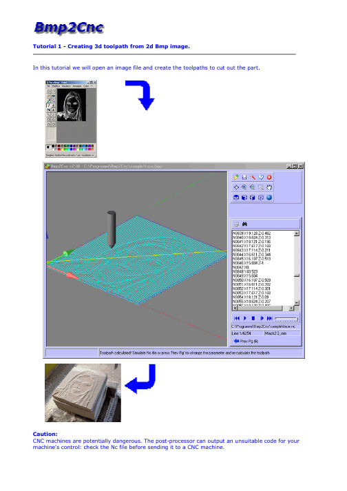
Caution:CNC machines are potentially dangerous. The post-processor can output an unsuitable code for your machine's control: check the Nc file before sending it to a CNC machine.1.Open the image file with the "Open" button.2.Select in "..\Bmp2Cnc\Sample\" folder the “face.bmp” file.3.The Dimension dialog will appear with the infos of image.4.Scale image to desidered dimension and press "Apply" button.5.Press "Next Pg" button.6.Define the reference point of image and press "Next Pg" button.6.The Depth dialog and 3d image will appear.Change the white and black depth value and press “Apply” button.Within graphics area, for change the view and / or magnification, use as follow To rotate: press left mouse button and move the mouse.To zoom: press CTRL + left mouse button and move the mouse.To pan: press SHIFT + left mouse button and move the mouse.7.Press "Next Pg" button.8.The NC file dialog will appear.Type "face" in the Windows file dialog.9.Select the postprocessor of your cnc machine.10.Press "Next Pg" button.11.In Tool definition press "Select" button to retrieve a tool from a tool library or create a new tool.12.Click in the Tool List to select the tool. Set feed and speed of the tool. Press the "OK" button.13.Press "Next Pg" button.14.The Cutting parameters page will appear. Set up the following parameters (this example work inmillimeters):15.Press the "Calculate" button.16.The toolpath is calculated and displayed together with the 3d image.17.Turn Off the shading: only the toolpath will be displayed.18.Press "Next Pg" button.19.The NC file text is diplayed.20.Press the "Play" button to simulate the toolpath (Yellow=Rapid, Cyan=Feed).21.You have successfully created your first Nc file with Bmp2Cnc.Caution:CNC machines are potentially dangerous. The post-processor can output an unsuitable code for your machine's control: check the Nc file before sending it to a CNC machine.。

TutorialLigandFittingwithCoot-CCP4：教程配体配合黑鸭-CCP4

Tutorial:Ligand Fitting with CootCCP4School APS2010May20,20101IntroductionWe have a protein structure(which is well-reﬁned).However,we have not yet identiﬁed the ligand position-indeed we don’t even know if the ligand is bound or not.In this tutorial,we will build a ligand and search the density for this ligand, add the ligand to main protein molecule and reﬁne and validate the ligand.2Experimental DetailsThis protein is the catalytic domain of poly(ADP-ribose)polymerase2crystallised from PEG3350(polyethylene glycol),Tris and cryoprotected using glycerol.3StartingSo let’s load the protein coordinates ligand-fitting-no-ligand.pdb and the associated MTZﬁle which is e File→AutoOpen MTZ.4SMILESNow what is the ligand that we want toﬁnd?It’s3-aminobenzamideFigure1:3-amino-benzamideHow do we make a3D model of this ligand?We use a SMILES string(and LIBCHECK).So what is the SMILES string for3-aminobenzamide?1available,as usual,from /coot/tutorial/If you can’t draw out the SMILES string,try this link in your browser:/cgi-bin/propertiesdraw the molecule there and hit the“Calculate Properties”button-the next pages gives you the SMILES string.We need to convert this SMILES string representation to a molecule.In Coot we do that using File→SMILES...2Enter you SMILES string in the second of the two entry boxes.Press”Go”.After a few moments(in which Coot runs LIBCHECK)a molecule will appear at the centre of the screen.Is it the molecule that you wanted?Note:check the hydrogens and planarity.5Fitting LigandsWe how the correct ligand now,So let’s move on to search the map for entities of this kind.Calculate→Other Modelling T ool→Find Ligands...We have2maps from which to choose.For now,let’s choose the2mFo-DFc map andﬁnd density clusters above1.0sigma.Make sure that you select the correct map and protein molecule and have selected the ligand that you made with the SMILES string.Press”Find’Em!”What do you see!?Y ou should see4hits.Let’s use the Fitted Ligands dialog to navigate to these hits.Do we like all the hits?If not,why not?Let’s worry about any problematicﬁttings later on and for now,let’s concentrate on the nicelyﬁtting solutions.If you like the any of the hits,merge them into the main protein molecule.Using Calculate→Merge Molecules,In the top pane,select the ligand hits thatﬁt nicely by ticking them.In the lower option menu,select the protein model.Then click”Merge”.Now we have 2representations of the ligands,which can be confusing,so let’s use the Display Manager to undisplay the Fitted Ligands that we merged into the main protein.Using the Fitted Ligand dialog,navigate to the newly added monomers and optimise theﬁt to density-we’ll use Real Space Reﬁnement to do e the blue target on right-hand toolbar and click an atom in the residue twice.Do you like the result of the reﬁnement?What is the torsion angle of the carboxy-amine? 6PresentationWe can emphasise the atom positions using Extensions→Representations→Hi-light Interesting Site.Nice?Maybe...2Note that theﬁrst line is the three letter code,conventionally this is3uppercase letters,e.g.LIG, DRG,XXX.Note that if you use several different SMILES strings,they each should have a different 3-letter-code.7Problem AreasOK,now we haveﬁtted the nicelyﬁtting ligands,let’s go back to the problematic blobs.Validate→Find unmodelled blobsWe shall search the2mFo-DFc as did previously using the same protein model (which now has the3-aminobenzamideﬁtted).Press”Find blobs”3 We should get a dialog with two blobs listed.Examine those two blobs.We know that3-aminobenzamide does notﬁt these blobs well.What else could these blobs be?Let’s look at the crystallization and freezing conditions?Any clues?Now,we don’t necessarily know the3-letter-codes of the molecules that might ﬁt these blobs.We can use the searching tool in Coot to convert between a molecule name and its3-letter-code.File→Search Monomer Library...add the molecule name to the entry box and press”Search”You will see a list of molecule that include the text you typed as part of the molecule names.If you click on any of those buttons,Coot runs LIBCHECK and generates a molecule and puts it at the centre of the screen.You can do this for the3or4different molecules that you think this blob might be.The centre of the screen is a bit crowded now.Undisplay those new ligands.To easily identify the bestﬁtting ligand at the site,let’s do ligandﬁtting here.Calculate→Other Modelling T ools→Find LigandsSelect the2mFo-DFc map as usual,and the main protein as before and the ligands to search for are the3or4newly created ligands.This time we will Search”Right Here”.You can turn onﬂexible ligands if you like,but this will slow down the search considerably.8Tidying UpReal Space reﬁnement is the tool to tidy things ing the blue circle icon on the right,then click click on an atom in the residue4.When we are happy with ourﬁt,we can merge this new ligand into the main protein ligand as we did before.9NCS LigandsYou may have noticed by now that there are2protein chains related by non-crystallographic symmetry.We can exploit this NCS to helpﬁt ligands.We have ﬁtting a ligand that bound to the”A”chain,now let’s use NCS to position a ligand in related position in the”B”chain of the protein.Extensions→NCS→NCS Ligands...The protein with the NCS is the main protein as usual,the molecule containing the ligand is also the main protein as usual(if we have done the merge mentioned above).We need to know the chain ID of the ligand that we haveﬁtted into the ”A”chain,to do that double left-click an an atom in the ligand.In the graphics you will see something like:"C1/1XXX/E"-so the chain-id is"E".Also the status bar at the bottom shows information about the clicked atom.3we could also use Validate→Difference Map Peaks to navigate to these positions.4or(quicker)simply press the”R”key(if you have the key bindings set up).So enter that chain-id in the”Molecule containing ligand””Chain ID”entry. Then”Find Candidate positions”.Aﬁtted ligands dialog box pops up and you can use the buttons in that dialog to navigate to the NCS ligand positions.Reﬁne this NCS ligand position if needed and merge it into the main molecule. 10For the AdventurousIf you are feeling adventurous,you can run refmac:Calculate→Model/Fit/Reﬁne →Run Refmac...Choose an MTZﬁle for Refmac and use theﬁle selector to choose the same MTZﬁle that we used in the beginning.Examine the resulting molecule.Are there any problems left toﬁx?。

GWT Tutorial

Lars Vogel Version 1.9 Copyright © 2008 - 2010 Lars Vogel 06.08.2010 GWT Tutorial This article describes how to develop a Web application with GWT and the Google Plugin for Eclipse. This article assumes basic Eclipse and Java knowledge . The article was developed using JDK 1.6, GWT 2.0and Eclipse 3.6 (Helios)). Table of Contents 1. Overview 1.1. Google Web Toolkit 1.2. Modules, Entry Points and HTML pages 1.3. Using CSS 2. Installation of the Google Tools for Eclipse 3. Create your first GWT application 3.1. Project 3.2. GWT entry point 3.3. HTML page 3.4. web.xml 3.5. Modify CSS 3.6. Run 4. GWT Project Structure 4.1. Overview 4.2. Module Descriptor 4.3. Entry point5. Debugging GWT applications6. Client and Server Communication (RPC)6.1. Overview6.2. Create project and domain model6.3. InterfaceHome Blog Java Eclipse Google Web Technology AlgorithmsRevision HistoryRevision 0.103.04.2007Lars Vogel / Waldemar Geppart Created with GWT 1.4Revision 0.2 - 1.911.10.2008 - 06.08.2010 Lars Vogelbugfixes and enhancements www SmartClient com/SmartGWT Ads by Google GWT Tutorial6.4. Create the server6.5. Define servlet in web.xml6.6. UI component - Table6.7. Callback6.8. Create your entry point6.9. Run7. UIBinder8. Using external jars / Java projects in GWT8.1. Overview8.2. Create the module project8.3. Use the module in another project9. Build your own components10. Thank you11. Questions and Discussion12. Links and Literature12.1. GWT resources1.1. Google Web ToolkitThe Google Web Toolkit (GWT) is a toolkit to develop Ajax web application with Java. The developer can develop in Java and debug the code. Once the code is finished, the GWT compiler translates the Java code into Javascript. This compiler compiles browser specific to make sure that all the major browsers are correctly support. GWT supports a standard set of UI widgets, a mechanism to support stateful behavior in the browser (support of the back button) and a JUnit based test framework.GWT provides two modesz Development Mode: allows to debug the Java code of your application directly via the standard Java debugger.zWeb mode: the application is translated into HTML and Javascript code and can be deployed on a webserver. 1.2. Modules, Entry Points and HTML pagesGWT applications are described as so-called modules. A module "modulename" is described by aconfiguration file "modulename.gwt.xml". Each module can define one or more Entry point classes. An entry point in GWT is the starting point for a GWT application similar to the main method in a standard Java program.The module is connected with an HTML page, which is called "host page". The code for a GWT webapplication executes within this HTML document. The HTML page can define "div" containers to which the GWT application can assign UI components. Alternatively the GWT UI components can be assigned to the body of the HTML page.1.3. Using CSSThe look and feel of a GWT application can be customized via CSS files. Each widget in GWT can be given a div container by using the method setStyle(String s); We will see later how this is used.Google offers a Eclipse plugin that provides both Google App Engine and GWT development capabilities. SWT Grid widget Fast and flexible Grid and TreeList with grouping and dynamic rendering Budget Portlets Get Customized Portlet Development Save on Portlet Building Costs /servicesPartner:Make Technologies Join Make Technologies in growing legacy system replacement industrywww.maketechnolo 1. Overview 2. Installation of the Google Tools for EclipseInstall the plugins from /eclipse/plugin/3.6 via the Eclipse update manager .The installation will also setup the GWT and App Engine SDK into your Eclipse preferences. To check this use Window -> Preferences -> Google -> App Engine / Web Toolkit. The SDK are delivered as plugins is included in your Eclipse installation directory under "/plugins/".3. Create your first GWT applicationThe following is a description of the usage of the Google plugin to create a new GWT application. plugin.3.1. ProjectSelect File > New > Web Application Project. Enter the name "de.vogella.gwt.helloworld" for your project and the java package. Only select "Use Google Web Toolkit", as we will not use the Google App Engine in this tutorial.Unfortunately the Google Plugin does not allow to created a new Web Application Projectwithout creating template files. The template files are nice for the first try but annoying ifyou want to start from scratch with a new GWT application. Please stare / vote for bugIssue 1547 to get this solved.Delete all java files under the package "client" and "server".3.2. GWT entry pointCreate a following Java class "HelloGwt" in the "de.vogella.gwt.helloworld.client" package.package de.vogella.gwt.helloworld.client;import com.google.gwt.core.client.EntryPoint;import com.google.gwt.event.dom.client.ClickEvent;import com.google.gwt.event.dom.client.ClickHandler;import er.client.Window;import er.client.ui.Button;import bel;import er.client.ui.RootPanel;public class HelloGwt implements EntryPoint {@Overridepublic void onModuleLoad() {Label label = new Label("Hello GWT !!!");Button button = new Button("Say something");{ClickHandler()button.addClickHandler(new@Overridepublic void onClick(ClickEvent event) {again");Window.alert("Hello,}});RootPanel.get().add(label);RootPanel.get().add(button);}}Create the file "De_vogella_gwt_helloworld.gwt.xml" in package "de.vogella.gwt.helloworld" to the following.<?xml version="1.0" encoding="UTF-8"?><module rename-to='de_vogella_gwt_helloworld'><inherits name='er'/><inherits name='er.theme.standard.Standard'/><entry-point class='de.vogella.gwt.helloworld.client.HelloGwt'/></module>This file defines your entry point to your application. In GWT the entry point is similar to the main method in Java.3.3. HTML pageIn the folder war/WEB-INF you should find a folder with the file "De_vogella_gwt_helloworld.html". Change this file to the following.<!DOCTYPE HTML PUBLIC "-//W3C//DTD HTML 4.01 Transitional//EN"><html><head><meta http-equiv="content-type" content="text/html; charset=UTF-8"><link type="text/css" rel="stylesheet" href="De_vogella_gwt_helloworld.css"><title>My First GWT applicaton</title><script type="text/javascript" language="javascript"src="de_vogella_gwt_helloworld/de_vogella_gwt_helloworld.nocache.js"></script></head><body><iframe src="javascript:''" id="__gwt_historyFrame" tabIndex='-1'style="position:absolute;width:0;height:0;border:0"></iframe><h1>My First GWT applicaton</h1></body></html>Please note that the HTML files points to the generate JavaScript file in the script tag. Ifyou using a different project name you need to adjust the path.3.4. web.xmlThe Google Plugin created also a web.xml and placed a reference to a servlet (which we deleted). Change the web.xml to the following.<?xml version="1.0" encoding="UTF-8"?><!DOCTYPE web-appPUBLIC "-//Sun Microsystems, Inc.//DTD Web Application 2.3//EN""/dtd/web-app_2_3.dtd"><web-app><welcome-file-list><welcome-file>De_vogella_gwt_helloworld.html</welcome-file></welcome-file-list></web-app>3.5. Modify CSSChange the CSS of our application. In folder war you find a file "De_vogella_gwt_helloworld.css". Change it to the following.h1 {font-size: 2em;font-weight: bold;color: #777777;}.gwt-Label {#DF0101;color:font: normal 12px tahoma, arial, helvetica, sans-serif;border: 1px solid #99bbe8;14px;padding:}.gwt-Button {5.7em;height:5px;margin-bottom:3px;padding-bottom:12px;font-size:font-family: arial, sans-serif;}The css file is referred to by the HTML page.You can assign a certain style to your GWT UI elements by using the "setStyleName"-Method as shown below.package de.vogella.gwt.helloworld.client;import com.google.gwt.core.client.EntryPoint;import com.google.gwt.event.dom.client.ClickEvent;import com.google.gwt.event.dom.client.ClickHandler;import er.client.Window;import er.client.ui.Button;import bel;import er.client.ui.RootPanel;public class HelloGwt implements EntryPoint {@Overridepublic void onModuleLoad() {Label label = new Label("Hello GWT !!!");label.setStyleName("my_label_for_css"); // Change css to use thisButton button = new Button("Say something");{ClickHandler() button.addClickHandler(new@Overridepublic void onClick(ClickEvent event) {again");Window.alert("Hello,}});RootPanel.get().add(label);RootPanel.get().add(button);}}3.6. RunTo run your application right-click the project and select Run As -> "Web application".This opens a new view "Development Mode. Copy the url from this view.Paste this url in your browser and install the required plugin (is necessary).The result should look like this:Congratulations! You created your first GWT application.4.1. OverviewIf you investigate your example from the last chapter you will see the following project structure.Flexess Easily create and manage user access rights in Java applications. Interface Module Interface Module[72] RT-SIC-1ADSL-H In Stock.Same Day Shipping Nirvana Middleware Unified Realtime Middleware for Enterprise,Web and Mobile Streaming 4. GWT Project StructureAn GWT application consists out of the following partsz Module descriptor: XML file which specifies mainly the entry point of the application. It has the name of your module plus .gwt.xmlz war: Under the folder "war" you find the HTML page which contains the GWT application. Additional public resources, e.g. other HTML pages, images or css files should be stored here. Here you find also the standard WEB-INF folder.z Source code: under your default package your find a package "client" All Java code which iscompiled for the client (Webbrowser) must be stored under client. For the service you would use the package "server".4.2. Module DescriptorThe main purpose of the Module descriptor in *.gwt.xml file is to define your entry-point. It also and defines standard GWT css styles which you are using.<?xml version="1.0" encoding="UTF-8"?><!DOCTYPE module PUBLIC "-//Google Inc.//DTD Google Web Toolkit 1.6.4//EN" "/svn/tags/1.6.4/distro-source/core/src/gwt-module.dtd"><module rename-to='de_vogella_gwt_helloworld'><inherits name='er'/><inherits name='er.theme.standard.Standard'/><entry-point class='de.vogella.gwt.helloworld.client.HelloGwt'/></module>4.3. Entry pointAn entry point in GWT is the starting point for a GWT application, similar to the main method in standard Java program. Every java class which is an entry point must implement the interface"com.google.gwt.core.client.EntryPoint" which defines one method onModuleLoad().Debugging a GWT application in development mode is easy. In this case you can just debug the Java code. Put a breakpoint into your coding and start the debugger via selecting your project, right-mouse click -> debug as -> Web Application.You can then use standard Eclipse debugging capabilities. Please see Eclipse Debugging for details.6.1. OverviewGWT provides its own remote procedure calls (RPC's) which allow the GWT client to call server-side methods. The implementation of GWT RPC is based on the servlet technology. GWT allows Java objects to be sent directly between the client and the server; which are automatically serialized by the framework. With GWT RPC the communication is almost transparent for the GWT client and always asynchronous so that the client does not block during the communication.The server-side servlet is usually referred to as a "service" and the a remote procedure call is referred to as "invoking a service." These object can then be used on the client (UI) side.To create a GWT service you need to define the following:z An interface which extends RemoteService that lists the service methods.z An implementation - implements the interface and extends the RemoteServiceServlet.zDefine an asynchronous interface to your service which will be used in the client code 6.2. Create project and domain modelCreate a GWT project "de.vogella.gwt.helloserver" with the package "de.vogella.gwt.helloserver". Create the following class which represents the data model . This class implements "Serializable" because GWT requires that all classes that are involved in a server and client communication have to implement the interface "Serializable".package de.vogella.gwt.helloserver.client.model;import java.io.Serializable;public class MyUser implements Serializable {private static final long serialVersionUID = 1L;private String id;private String username;private String numberOfHits;public String getId() {return id;}public void setId(String id) {this.id = id;}public String getUsername() {return username;} Ads by Google Eclipse GWT Stress Framework GWT GWT Web 2.0 5. Debugging GWT applications 6. Client and Server Communication (RPC)public void setUsername(String username) {username;ername=}/*** @return the numberOfHits*/public String getNumberOfHits() {numberOfHits;return}/*** @param numberOfHits* the numberOfHits to set*/public void setNumberOfHits(String numberOfHits) {numberOfHits;=this.numberOfHits}//}6.3. InterfaceThe client server communication is based on an interface which defines the possible communication methods.Create the following interface. By extending the RemoteService interface the GWT compiler will understand that this interface defines an RPC interface. The annotation defines the URL for the service. This must match the entry we will later do in "web.xml".package de.vogella.gwt.helloserver.client.service;import java.util.List;import er.client.rpc.RemoteService;import er.client.rpc.RemoteServiceRelativePath;import de.vogella.gwt.helloserver.client.model.MyUser;//@RemoteServiceRelativePath("userService")public interface MyUserService extends RemoteService {getUserList();List<MyUser>MyUser getUser(String id);}This interface needs to be available on the client side, therefore it must be placed in theclient package.GWT uses asynchronous communication therefore you also need to create the asynchronous version of this interface. The name of this interface must be the interface name concatenated with "Async".package de.vogella.gwt.helloserver.client.service;import java.util.List;import er.client.rpc.AsyncCallback;import de.vogella.gwt.helloserver.client.model.MyUser;public interface MyUserServiceAsync {void getUserList(AsyncCallback<List<MyUser>> callback);void getUser(String id, AsyncCallback<MyUser> callback);}The implementation of this asynchronous interface will be automatically created by theGWT compiler.6.4. Create the serverFor the server implementation create a package "de.vogella.gwt.helloworld.server". Create the following class which extends RemoteServiceServlet.package de.vogella.gwt.helloserver.server;import java.util.ArrayList;import java.util.List;import er.server.rpc.RemoteServiceServlet;import de.vogella.gwt.helloserver.client.model.MyUser;import de.vogella.gwt.helloserver.client.service.MyUserService;public class MyUserServiceImpl extends RemoteServiceServlet implements{MyUserServiceprivate static final long serialVersionUID = 1L;private List<MyUser> userList = new ArrayList<MyUser>();public MyUserServiceImpl() {MyUser user = new MyUser();user.setId("1");user.setUsername("Peter");user.setNumberOfHits("15");userList.add(user);newMyUser();=useruser.setId("2");user.setUsername("Hanz");user.setNumberOfHits("25");userList.add(user);}public MyUser getUser(String id) {for (Object object : userList) {object).getId().equals(id))(((MyUser)ifobject);((MyUser)return}null;return}public List<MyUser> getUserList() {userList;return}}6.5. Define servlet in web.xmlTo make GWT aware of this service change the web.xml file in war/WEB-INF to the following.:<?xml version="1.0" encoding="UTF-8"?><!DOCTYPE web-appPUBLIC "-//Sun Microsystems, Inc.//DTD Web Application 2.3//EN""/dtd/web-app_2_3.dtd"><web-app><welcome-file-list><welcome-file>De_vogella_gwt_helloserver.html</welcome-file></welcome-file-list><servlet><servlet-name>userServlet</servlet-name><servlet-class>de.vogella.gwt.helloserver.server.MyUserServiceImpl</servlet-class> </servlet><servlet-mapping><servlet-name>userServlet</servlet-name><url-pattern>/de_vogella_gwt_helloserver/userService</url-pattern></servlet-mapping></web-app>6.6. UI component - TableCreate the following two classes which will be used to display the data in a table. The implementation of "MyTable" is based on FlexTable. FlexTable allows the building of tables in GWT.package de.vogella.gwt.helloserver.client.table;import java.util.ArrayList;import java.util.List;import de.vogella.gwt.helloserver.client.model.MyUser;public class DataSource {private final List<MyUser> users;private List<String> header;public DataSource(List<MyUser> users) {header = new ArrayList<String>();header.add("Id");header.add("Name");Hits");ofheader.add("Numberusers;=ers}public List<MyUser> getUsers() {users;return}public List<String> getTableHeader() {header;return}}package de.vogella.gwt.helloserver.client.table;import java.util.List;import er.client.ui.FlexTable;import de.vogella.gwt.helloserver.client.model.MyUser;public class MyTable extends FlexTable {DataSourceinput;public MyTable(DataSource input) {super();this.setCellPadding(1);this.setCellSpacing(0);this.setWidth("100%");this.setInput(input);}public void setInput(DataSource input) {for (int i = this.getRowCount(); i > 0; i--) {this.removeRow(0);}if (input == null) {return;}int row = 0;List<String> headers = input.getTableHeader();if (headers != null) {int0;=ifor (String string : headers) {i,string);this.setText(row,i++;}row++;}// Make the table header look nicer"tableHeader"); this.getRowFormatter().addStyleName(0,List<MyUser> rows = input.getUsers();int i = 1;for (MyUser myUser : rows) {myUser.getId());this.setText(i,0,myUser.getUsername());this.setText(i,1,myUser.getNumberOfHits());2,this.setText(i,i++;}this.inputinput;=}}6.7. CallbackTo receive a callback a class needs to be implemented which can then react on a failure or success in the communication. The interface AsyncCallback defines these two methods: "OnSuccess" and "OnFailure".Keep in mind that the server communication is asynchronous. If you call your server yourGWT application will continue and at some undefined point in time it will receive the datafrom the server. Make sure that you do not assume in your coding that the call to theserver is finished.Create the following class.package de.vogella.gwt.helloserver.client.service;import java.util.List;import er.client.Window;import er.client.rpc.AsyncCallback;import de.vogella.gwt.helloserver.client.model.MyUser;import de.vogella.gwt.helloserver.client.table.DataSource;import de.vogella.gwt.helloserver.client.table.MyTable;/*** Class which handles the asynchronous callback from the server* <p>* Need to react on server communication failure and success** @author Lars Vogel**/public class MyUserCallback implements AsyncCallback<List<MyUser>> {private MyTable table;public MyUserCallback(MyTable table) {table;this.table=}public void onFailure(Throwable caught) {Window.alert(caught.getMessage());}public void onSuccess(List<MyUser> result) {result;=List<MyUser>usersDataSource datasource = new DataSource(users);table.setInput(datasource);for (MyUser user : users) {System.out.println(user.getUsername());}}}This will simple print the received results to the command line.6.8. Create your entry pointCreate the following class.package de.vogella.gwt.helloserver.client.entrypoint;import com.google.gwt.core.client.EntryPoint;import com.google.gwt.core.client.GWT;import com.google.gwt.event.dom.client.ClickEvent;import com.google.gwt.event.dom.client.ClickHandler;import er.client.rpc.ServiceDefTarget;import er.client.ui.Button;import er.client.ui.DialogBox;import er.client.ui.RootPanel;import er.client.ui.VerticalPanel;import de.vogella.gwt.helloserver.client.service.MyUserCallback;import de.vogella.gwt.helloserver.client.service.MyUserService;import de.vogella.gwt.helloserver.client.service.MyUserServiceAsync;import de.vogella.gwt.helloserver.client.table.MyTable;/*** Entry point classes define <code>onModuleLoad()</code>.*/public class HelloServer implements EntryPoint {private MyTable table;/*** This is the entry point method.*/public void onModuleLoad() {table = new MyTable(null);Button button = new Button("Click me");// We can add style namesbutton.addStyleName("pc-template-btn");// or we can set an id on a specific element for stylingVerticalPanel vPanel = new VerticalPanel();vPanel.setWidth("100%");vPanel.setHorizontalAlignment(VerticalPanel.ALIGN_CENTER);vPanel.add(button);vPanel.add(table);// Add table and button to the RootPanelRootPanel.get().add(vPanel);// Create the dialog boxfinal DialogBox dialogBox = new DialogBox();dialogBox.setText("Welcome to GWT Server Communication!");dialogBox.setAnimationEnabled(true);Button closeButton = new Button("close");VerticalPanel dialogVPanel = new VerticalPanel();dialogVPanel.setWidth("100%");dialogVPanel.setHorizontalAlignment(VerticalPanel.ALIGN_CENTER);dialogVPanel.add(closeButton);{ClickHandler()closeButton.addClickHandler(new@Overridepublic void onClick(ClickEvent event) {dialogBox.hide();}});// Set the contents of the WidgetdialogBox.setWidget(dialogVPanel);ClickHandler(){button.addClickHandler(new@Overridepublic void onClick(ClickEvent event) {GWT(MyUserServiceAsync) MyUserServiceAsyncservice=.create(MyUserService.class);ServiceDefTargetservice;(ServiceDefTarget)serviceDef=serviceDef.setServiceEntryPoint(GWT.getModuleBaseURL()"userService");+MyUserCallback(table);new=MyUserCallbackmyUserCallbackservice.getUserList(myUserCallback);}});}}Define your entry point in "De_vogella_gwt_helloserver.gwt.xml".<?xml version="1.0" encoding="UTF-8"?><!DOCTYPE module PUBLIC "-//Google Inc.//DTD Google Web Toolkit 1.6.4//EN" "/svn/tags/1.6.4/distro-source/core/src/gwt-module.dtd"><module rename-to='de_vogella_gwt_helloserver'><inherits name='er'/><inherits name='er.theme.standard.Standard'/><entry-point class='de.vogella.gwt.helloserver.client.entrypoint.HelloServer'/></module>Change your "De_vogella_gwt_helloserver.html" page to the following.<!DOCTYPE HTML PUBLIC "-//W3C//DTD HTML 4.01 Transitional//EN"><html><head><meta http-equiv="content-type" content="text/html; charset=UTF-8"><link type="text/css" rel="stylesheet" href="De_vogella_gwt_helloserver.css"><title>Web Application Starter Project</title><script type="text/javascript" language="javascript"src="de_vogella_gwt_helloserver/de_vogella_gwt_helloserver.nocache.js"></script></head><body></body></html>Also change the "De_vogella_gwt_helloserver.css" to the following to make the table header look nicer.body {padding: 10px;}/* stock list header row */.tableHeader {background-color: #2062B8;color: white;font-style: italic;}6.9. RunRun your application. If you click the button then a list of users on click should get loaded.The eclipse console shows the values of the users send to your Google Web application via the service.7. UIBinderUIBinder allows to design GWT UI's declarative via XML.Create a new GWT project "de.vogella.gwt.uibinder" with the package "de.vogella.gwt.uibinder".To use UIBinder you also need to inherit from "com.google.gwt.uibinder.UiBinder" in your "gwt.xml" file.<?xml version="1.0" encoding="UTF-8"?><module rename-to='de_vogella_gwt_uibinder'><inherits name='er' /><inherits name='com.google.gwt.uibinder.UiBinder' /><inherits name='er.theme.standard.Standard' /><entry-point class='de.vogella.gwt.uibinder.client.De_vogella_gwt_uibinder' /><source path='client' /></module>In your client package create the file "HelloWidgetWorld.ui.xml".<ui:UiBinder xmlns:ui='urn:ui:com.google.gwt.uibinder'xmlns:g='urn:import:er.client.ui'><g:VerticalPanel><g:HorizontalPanel>2</g:Label><g:Label>Label<g:TextBoxText</g:TextBox>ui:field='text1'>Some</g:HorizontalPanel><g:HorizontalPanel></g:Label><g:Label>Label2Text</g:TextBox> <g:TextBoxui:field='text2'>More</g:HorizontalPanel><g:ListBox ui:field='listBox' visibleItemCount='1' /><g:Button ui:field='submit'> Submit </g:Button></g:VerticalPanel></ui:UiBinder>Create the following class which uses the xml file for building actions. By convention the name of the xml must equal to the class name + "ui.xml".package de.vogella.gwt.uibinder.client;import com.google.gwt.core.client.GWT;import com.google.gwt.event.dom.client.ClickEvent;import com.google.gwt.uibinder.client.UiBinder;import com.google.gwt.uibinder.client.UiField;import com.google.gwt.uibinder.client.UiHandler;import com.google.gwt.uibinder.client.UiTemplate;import er.client.Window;import er.client.ui.Button;import posite;import er.client.ui.ListBox;import er.client.ui.Widget;public class HelloWidgetWorld extends Composite {// Annotation not needed as we use the default but this allows to change the path @UiTemplate("HelloWidgetWorld.ui.xml")interface MyUiBinder extends UiBinder<Widget, HelloWidgetWorld> { }private static MyUiBinder uiBinder = GWT.create(MyUiBinder.class);。

1、下载文档前请自行甄别文档内容的完整性，平台不提供额外的编辑、内容补充、找答案等附加服务。
2、"仅部分预览"的文档,不可在线预览部分如存在完整性等问题,可反馈申请退款(可完整预览的文档不适用该条件!)。
3、如文档侵犯您的权益，请联系客服反馈,我们会尽快为您处理(人工客服工作时间：9:00-18:30)。

Coot TutorialCCP4School APS2010May20,2010Contents1Mousing2 2Introductory T utorial22.1Get theﬁles (2)2.2Start Coot (2)2.3Display Coordinates (2)2.4Adjust Virtual Trackball (3)2.5Display maps (4)2.6Zoom in and out (5)2.7Recentre on Different Atoms (5)2.8Change the Clipping(Slab) (7)2.9Recontour the Map (7)2.10Change the Map Colour (8)2.11Select a Map (8)3Model Building83.1Rotamers (8)3.2More Real Space Reﬁnement (9)4Blobology104.1Find Blobs (10)4.1.1Blob3 (10)4.1.2Blob2 (11)4.1.3Blob1 (12)5Extra Fun(if you have time)125.1Waters (12)5.2Working with NCS (13)5.3Add Terminal Residue (14)5.4Display Symmetry Atoms (15)5.5Skeletonization and Baton Building (16)5.6Reﬁne with Refmac (16)6Use the EDS166.1Make a(Pretty?)Picture (17)1MousingFirst,how do we move around and select things?Left-mouse Drag Rotate viewCtrl Left-Mouse Drag Translates viewShift Left-Mouse Label AtomRight-Mouse Drag Zoom in and outMiddle-mouse Centre on atomScroll-wheel Forward Increase map contour levelScroll-wheel Backward Decrease map contour level2Introductory T utorialIn this tutorial,we will learn how to do the following:1.Start Coot2.Display coordinates3.Display a map4.Zoom in and out5.Recentre on Different Atoms6.Change the Clipping(Slab)7.Recontour the Map8.Change the Map Colour9.Display rotamers and reﬁne residue2.1Get theﬁlesBefore we start,let’s get theﬁles on which we will be working:$wget /coot/tutorial/tutorial-modern.pdb$wget /coot/tutorial/rnasa-1.8-all refmac1.mtz or copy them from/home/emsley/tutorial2.2Start CootTo use coot,in a terminal window,type:$cootWhen youﬁrst start coot,it should look something like Figure1.2.3Display CoordinatesSo let’s read in those coordinates:•Select“File”from the Coot menu-bar11Note you can also use“Alt-F”instead of clicking on“File”Figure1:Coot at StartupNot much to see at present...Actually,after this,coot screenshots will bedisplayed with a white background,whereas you will see a black one•Select the“Open Coordinates”menu item[Coot displays a Coordinates File Selection window]•Either–Select tutorial-modern.pdb from the“Files”listor–Type tutorial-modern.pdb in the Selection:entry•Click“OK”in the Coordinates File Selection window[Coot displays the coordinates in the Graphics Window]2.4Adjust Virtual TrackballBy default,Coot has a“virtual trackball”to relate the motion of the molecule to the motion of the mouse.Many people don’t like this.So you might like to try the following.In the Coot main menu-bar:Edit→Preferences...[Coot displays a Preferences window]On the left toolbar select General and then on the right top notebook tab HID. Select“Flat”to change the mouse motion.(Use the“Spherical Surface”option to turn it back to how it is by default).What is the difference?“Flat”mode is like the mode used by“O”.In both modes,dragging the mouse near the centre of the screen causes the view to rotate about the X-or Y-axis.However in spherical mode you can also rotate about thez-axis by dragging the mouse along an edge of the window.Figure2:Coot After Loading Coordinates2.5Display mapsWe are at the stage where we are looking at the results of the reﬁnement.The reﬁnement programs stores its data(labelled lists of structure factor amplitudes and phases)in an“MTZ”ﬁle.Let’s take a look...•Select“File”from the Coot menu-bar•Select“Auto Open MTZ”menu item[Coot displays a Dataset File Selection window]•Select theﬁlename rnasa-1.8-all refmac1.mtzIf you choose instead“Open MTZ,cif or phs...”you will see:•[Coot displays a Dataset File Selection window]•Select theﬁlename rnasa-1.8-all refmac1.mtz[Coot displays a Dataset Column Label Selection window]Figure3:Coot MTZ Column Label Selection Window Notice that you have a selection of different column labels for the“Ampli-tudes”and“Phases”,however,let’s use the defaults:“FWT”and“PHWT”.•Press“OK”in the Column Label WindowNow open the MTZﬁle and select column labels“DELFWT”and“PHDELWT”.So now we have2maps(whether auto-opened or not).2.6Zoom in and outTo zoom in,click Right-mouse and drag it left-to-right2.To zoom out again,move the mouse the opposite way.Figure4:Coot after reading an MTZﬁle and zoomed in.2.7Recentre on Different Atoms•Select“Draw”from the Coot menu-bar•Select“Go T o Atom...”[Coot displays the Go To Atom window]•Expand the tree for the“A”chain•Select1ASP in the residue list•Click“Apply”in the Go To Atom window•At your leisure,use“Next Residue”and“Previous Residue”(or“Space”and “Shift”“Space”in the graphics window)to move along the chain.•Click Middle-mouse over an atom in the graphics window[Coot recentres on that atom]•Ctrl Left-mouse&Drag moves the view around.If this is a too slow and jerky:–Select Edit→Preferences...from Coot’s menu-bar–Select the“Maps”toolbutton on the left2or up-to-down,if you prefer that–Select the“Dragged Map”notebook tab.–Select“No”in the“Active Map on Dragging”window–Click“OK”in the“Preferences”windowNow the map is recontoured at the end of the drag,not at each step3.Another,additional way to make the movements faster is to change the num-ber of steps for the“Smooth Recentering”.Again youﬁnd this in the“Prefer-ences”(Preferences→General→Smooth Recentering).Change the“Num-ber of Steps”from the default80to something smaller,e.g.20.Figure5:Coot’s Go To Atom Window.•You can display the contacts too,as you do this:–Select“Measures”from the Coot menu-bar–Select“Environment Distances...”–Click on the“Show Residue Environment?”check-button∗Also Click“Label Atom?”if you wish the Cαatoms of the residuesto be labelled.–Click“OK”in the Environment Distances window–Click“Apply”in the Go To Atom window[You can’t change the colour of the Environment distances]You can turn off the Environment distances if you like.3which looks less good on faster computers.Figure6:Coot showing Atom Label and environment distances.2.8Change the Clipping(Slab)•Select“Draw”from the Coot menu-bar•Select“Clipping...”from the sub-menu[Coot displays a Clipping window]•Adjust the slider to the clipping of your choice•Click“OK”in the Clipping windowAlternatively,you can use“D”and“F”4on the keyboard,or Control Right-mouse up/down(Control Right-mouse left/right does z-translation).2.9Recontour the Map•Scroll your scroll-wheel forwards one click5[Coot recontours the map using a0.05electron/˚A3higher contour level]•Scroll your scroll-wheel forwards and backwards more notches and see the contour level changing.•If you don’t have a wheel on your mouse you can use“+”and“-”on the keyboard.•Note that the“Scroll”button in the Display Manager allows you to select which map is affected by this6.4think:Depth of Field.5don’t click it down.6by default it is the last map,which is not necessarily the map that you want.2.10Change the Map Colour•Select“Edit”from the Coot menu-bar•Select“Map Colour”in the sub-menu•Select“1xxx FWT PHWT”in the sub-menu[Coot displays a Map Colour Selection window]•Choose a new colour by clicking on the colour widgets[Coot changes the map colour to match the selection]•Click“OK”in the Map Colour Selection window2.11Select a MapSelect a map for model building:Menubar:Calculate→Model/Fit/Reﬁne...[Coot displays the Model/Fit/Reﬁne window]Select“Select Map...”from the Model/Fit/Reﬁne windowclick OK(you want to select the map with“...FWT PHWT”)Alternatively you can use the modelling toolbar icon buttons(here“Map”)dis-played on the right side of the Coot window.Most options found in the Model/Fit/Reﬁne window are available here too.If you are not sure which icon corresponds to which function look at the displayed tips when over the button with the mouse.Or change the display style of the buttons by clicking on the bottom arrow and select another style to get only or additionally text displayed.3Model Building“So what’s wrong with this structure?”you might ask.There are several ways to analyse structural problems and some of them are available in Coot.Validate→Density Fit Analysis→tutorial-modern.pdb[Coot displays a bar graph]Look at the graph.The bigger and redder the bar the worse the geometry.Thereare2area of outstanding badness in the A chain,around41A and89A.Let’s look at89Aﬁrst-click on the block for89A.[Coot moves the view so that89A CA is at the centre of the screen]3.1Rotamers•Examine the situation...[The sidechain is pointing the wrong way.Let’s Fix it...]•Menubar:Calculate→Model/Fit/Reﬁne (7)[Coot displays the Model/Fit/Reﬁne window]•Select“Rotamers”from the Model/Fit/Reﬁne window8.7or use the modelling toolbar on the right of the Coot window,i.e.you don’t need to open theModel/Fit/Reﬁne window8Or click on the“Rotamers”button of the modelling toolbar•In the graphics window,(left-mouse)click on an atom of residue89A(the Cγ,say)[Coot displays the“Select Rotamer”window]•Choose the Rotamer that most closely puts the atoms into the side-chain den-sity•Click“Accept”in the“Select Rotamer”window[Coot updates the coordinates to the selected rotamer]•Click“Real Space Reﬁne Zone”in the Model/Fit/Reﬁne window9.•In the graphics window,click on an atom of residue89A.Click it again.[Coot displays the reﬁned coordinates in white in the graphics and a new “Accept Reﬁnement”window]•Click“Accept”in the“Accept Reﬁnement”window.[Coot updates the coordinates to the reﬁned coordinates.89A nowﬁts the density nicely.]OK.That’s good.Now,how about if we just use Real Space Reﬁnement only?•Click“Undo”twice[Coot puts the sidechain back to the original position]•Click“Real Space Reﬁne Zone”in the Model/Fit/Reﬁne window10.•In the graphics window,click on an atom of residue89A.Click it again.[Coot displays the reﬁned coordinates in white in the graphics and a new “Accept Reﬁnement”window]•Now using left-mouse,click and drag on the intermediate(white)CZ atom of the PHE(if you mis-click the atom,the view will rotate).•Can you pull the atom around so that the side-chainﬁts the density?[Yes,you can]3.2More Real Space ReﬁnementNow let’s have a look at the other region of outstanding badness:•Click on the graph block for41A[Coot moves the view so that41A CA is at the centre of the screen]•Examine the situation...•Residue41is in a mess and notﬁtting to the density.Can youﬁx it?[Yes,you can]•The trick is Real Space Reﬁne that zone.So...9...or use the modelling toolbar button10...or modelling toolbar buttonFigure7:89A nowﬁts the density nicely.•You can either Real Space Reﬁne a few residues(40,41and42)or just41.Take your pick.•Click on“Real Space Reﬁne Zone”in the Model/Fit/Reﬁne window•Select a range by clicking on atoms in the graphics window(either atoms in 40then42or an atom in41twice)[Coot displays intermediate(white)atoms]•Click and drag on some atoms until the atomsﬁt nicely in the density.If you want to move a single atom then Ctrl Left-mouse to pick and move(just) that intermediate atom.[Note:Selecting and moving just the Carbonyl Oxygen is a good idea-use Ctrl Left-mouse to move just one atom.]4Blobology4.1Find BlobsTo be found under Validate(called“Unmodelled Blobs”).You can use the defaults in the subsequent pop-up.Press“Find Blobs”and wait a short while.You will get a new window that tell you that it has found unexplaned blobs. Time toﬁnd out what they are.4.1.1Blob3Let’s start from Blob3(the blobs are ordered biggest to smallest-Blobs3and4(if you have it)are the smallest).•Click on“Blob3”[Coot centres the screen on a blob]•Examine the situation...[We need something tetrahedral there...]•“Place Atom At Pointer”on the Model/Fit/Reﬁne window11[Coot shows a Pointer Atom Type window]•“SO4”in the new window...•In the“Pointer Atom Added to Molecule:”frame,change“New Molecule”to‘‘tutorial-modern.pdb”•Click OK.•Examine the situation...•the orientation is not quite right.•Let’s Real Space Reﬁne it(you should know what to do by now...)•(“Real Space Reﬁne Zone”then click an atom in the SO4twice.Accept)[The SO4ﬁts better now].Blob4is like Blob3(isn’t it?)4.1.2Blob2Click on the button“Blob2”and examine the density.Something is missing from the model.What?This protein and has been co-crystallized with its ligand substrate.That’s what missing:3’GMP.So let’s add it...•File→Get Monomer...•Type3GP in the box(Use Upper Case).Press return...[Coot pauses for a few seconds while LIBCHECK and REFMAC run][3GP appears]It is generally easier to work without hydrogens,so let’s delete them•“Delete...”from the Model/Fit/Reﬁne window12•“Hydrogens in Residue”•click on an atom in3GP[Hydrogens disappear]The3GP is displaced from where we want it to be.•“Rotate/T ranslate Zone”from the Model/Fit/Reﬁne window13•click on an atom in3GP twice[Intermediate(white)atoms appear]•Drag it or use the sliders to move the intermediate fragment to the approxi-mately the right place.11also available in the modelling toolbar12Found in the modelling toolbar?Of course!13Found it in the modelling toolbar?•Click“OK”in the slider window•Now optimize theﬁt using“Real Space Reﬁne Zone”like we did before.Now merge this ligand into the protein:•Calculate→Merge Molecules...•Click(activate)“monomer-3GP.pdb”•into Molecule:tutorial-modern.pdb•Merge4.1.3Blob1•Click on“Blob1”•Examine the situation...What is this density?[We need to add residues to the C-terminus of the A chain.]The missing residues are GLU,THR,CYS(QTC).•Calculate→Fit Loop...[Coot pops-ups a Fit Loop dialog]Add residue number94to96in the A chain.The single letter codes of the extra residues are QTC•Make sure that you can see the unmodelled density well,then click“Fit Loop”•Watch...(fun eh?)•Examine the densityﬁt.[It should beﬁne,except at the C-terminus.We need to add an OXT atom to the residue]•Calculate→Other Modelling T ools...•Add OXT to Residue...•Add it——————————————————This is a far as I expect you to get.——————————————————5Extra Fun(if you have time)5.1WatersFit waters to the structure•“Find Waters...”in the Other Modelling Tools dialog14,then OK(using the defaults)[Waters appear]14In older versions of Coot,the Find Waters button can be found in the Model/Fit/Reﬁne dialog or the water drop in the modelling toolbarTo check the waters:•Click on“Measures”in the main menubar.•Click on Environment Distances•Click on the“Show Residue Environment?”check-button•Change the distances as you like•Use the Go To Atom widget to go to theﬁrst water(probably towards the end of the list of residues in Chain“W”)•Use the Spacebar to navigate to the next residue(and Shift Spacebar to go backwards)•If you don’t like the fast sliding15you can turn it off(if you haven’t done so already):–Click Edit→Preferences...in the main menubar–Click General→“Smooth Recentering...”–Click“No”5.2Working with NCSThe tutorial data has two-fold NCS.With good data it is interesting to investigate the differences between the NCS copies.This may be done by comparing the NCS related electron density,comparing the NCS related chains,or comparing the Ra-machandran plots for related chains:•Comparing the NCS related electron density.Go to Calculate/NCS maps and select theﬁrst map and model.Now,if you go to anywhere in the A chain,you will see two sets of electron density-the original density for the A chain,and the density for the B chain transformed to overlap the A chain density.This gives you a visual comparison of any differences.Look at the density in the B molecule.Why does the density not agree here?(Hint:the NCS is not a2-fold rotation in this case,it is improper).•Comparing the NCS-related chains.Go to Draw/NCS ghost control and select Draw non-crystallographic ghosts.You will now see a copy of the B chain superimposed on the A chain.The B chain is draw using thin bonds.Look for regions where the models ing the NCS maps tool,check that the differences in the models are supported by the density.•Compare the NCS-related chains using“NCS jumping”.This is an alternative way of examining NCS similarities and e the Display Manager to undisplay the NCS maps you recently created above.Use the“Goto Atom”dialog and press the“Update from Current Position”button.[Coot shifts the centre of the screen to the closest displayed CA atom]15it’s not very good for water checkingIdentify the chain that you are looking at(for example,by double-clicking on an atom)Now press the“o”key on the keyboard.[Coot shifts the centre of the screen to a NCS-related chain]Identify the chain that you are looking at now.Press“o”again.What is happening?(Note:”o”stands for“Other NCS-related chain”.)•Comparing the Ramachandran plots for related chains.Go to Validate/Kleywegt plot.Check the Use speciﬁc chain options and select chains A and B.You will get a Ramachandran plot with equivalent residues from the A and B chains linked by arrows.Long arrows indicate signiﬁcant differences.Click on a dot to view the residue concerned.Another tool for identifying NCS differences is the Validate/NCS differences graph.This gives a clickable histogram of differences.5.3Add Terminal Residue[To be found on the Model/Fit/Reﬁne dialog16]•Use the Go To Atom window to go to residue72A.•What do you see?[You see missing atoms(that is,you don’t see them).This residue is supposed to bea CYS!Bad things have happened to it.Let’s get rid of this residue.][There may also be waters in the side-chain positions too(they have to be removed too).]•Delete...•(Make sure“Residue/Monomer”is active)•Click on an atom of residue72A.[Residue72A disappears]•Lets’put back an ALA.•Add Terminal Residue...[Coot adds intermediate white atoms and pops up a dialog]•Accept the new atomsOK,we now have a ALA.We want a CYS:•Mutate&Auto Fit...•Click on an atom in the new ALA[Coot pops up a residue type chooser]•Choose residue type CYS[Coot mutates andﬁts a CYS]16and in the modelling toolbar•Examine the situation.[There is an extra blob of density on that CYS.What is it?]It is an alternative conformation.Let’s model it•Add Alt Conf...[Coot pops up a residue splitter dialog]•Choose how you want to split your residue(the Right Way is an unresolved philosophical issue...17)•Click on an atom in72A[Coot adds intermediate white atoms and pops up a Rotamer Chooser]•Choose the correct rotamer-it shouldn’t be difﬁcult to tell which is the clos-est.•Accept when you are happy with you choice.•Now optimize theﬁt of this new residue with Real Space Reﬁnement.The reﬁnement of each alternate conformations is independent.•Real Space Reﬁne Zone•click on(say)SG,B of72A•Press“A”(on the keyboard)[Coot moves the atoms a bit]•Accept•Now do the same with the other conformation.[Ahhh!Much better.]5.4Display Symmetry AtomsTo be found on“Draw”→“Cell&Symmetry”menu item in the main menu.Try:•Show Symmetry Atoms?→Y es•Symmetry as Calphas?[on]•Colour symmetry by molecule[on]•Symmetry Radius30˚A•Colour Merge→0.1•Show Unit Cell?[on]•OK•Zoom out and have a look at how the molecules pack together.17Actually Jane Richardson may disagree with that statement.5.5Skeletonization and Baton BuildingYou can calculate the map skeleton in Coot directly:Calculate→Map Skeleton...→On.This can be used to“baton build”a map.You can turn off the coordinates and try it if you like(the Baton Building window can be found by clicking“Ca Baton Mode...”in the Other Modelling Tools dialog18).If you want to do this,I suggest you use Go To Atom and start residue2A(this allows you to build the complete A chain in the correct direction(it takes about15 minutes or so)and you can compare it to the real structure afterwards.Remember,when you start,you are placing a CA at the baton tip and at the start you are placing atom CA1.This might seem that you are“double-backing”on yourself-which can be confusing theﬁrst time.5.6Reﬁne with RefmacRefmac is a program that does Maximum Likelihood reﬁnement of the model,and the interface to it can be found on the Model/Fit/Reﬁne dialog.(By default there is no icon on the toolbar for this action-open the window from the calculate menu19). Now click on“Run Refmac...”(at the bottom of the Model/Fit/Reﬁne window).The defaults should beﬁne...“Run Refmac”in the new window......Wait...[The cycle continues...]•Use“Validate→Difference Map Peaks”toﬁnd interesting features in the newly created map and model.•Python enabled version only:a dialog with geometric outliers and other in-teresting things(if they exist)detected by Refmac shows up20.6Use the EDSLet’s validate a structure deposited in the PDB.Use a web browser and go to http://eds.bmc.uu.se/eds/.Use the keyword search toﬁnd the structure of a particular protein/ligand/author.File→Get PDB and Map Using EDSGet the accession code and paste it into the entry box that pops up.Use the validation tools in Coot to examine how good a PDBﬁle this is...[the Difference Map Peaks can be interesting]18this is quite advanced19or add your own“Run Refmac”button to the toolbar or the main/top toolbar.To add the button to the modelling/side toolbar,open the“Preference”window.Now go to Preferences→General→Reﬁnement T oolbar.In the right hand window scroll down and tick the box besides“Run Refmac...”.A corresponding button will appear on the modelling toolbar.Alternatively you can add your own “Run Refmac...”button to the top toolbar of the Coot window(only in Python versions).Click Right-mouse on the toolbar(besides the“Display Manager”button)and you will see a pop-up menu.Select “Manage Buttons”,tick the box besides“Add Alt Conf”and click“Apply”.A new button named“Add Alt Conf”will appear on the toolbar.20This is an analysis from the Refmac logﬁle and can alternatively be opened from Extensions...→Reﬁne...→Read REFMAC log6.1Make a(Pretty?)Picture(Depends on the appropriate supporting software being available):•Arrange a nice view•Press F8•Wait a few seconds...ColophonThis document is written using XEmacs21.5in L A T E X using AUCT E X and is dis-tributed with the Coot source code.。