《数据结构与算法分析》
数据结构与算法分析实验报告

数据结构与算法分析实验报告一、实验目的本次实验旨在通过实际操作和分析,深入理解数据结构和算法的基本概念、原理和应用,提高解决实际问题的能力,培养逻辑思维和编程技巧。
二、实验环境本次实验使用的编程语言为 Python,使用的开发工具为 PyCharm。
操作系统为 Windows 10。
三、实验内容(一)线性表的实现与操作1、顺序表的实现使用数组实现顺序表,包括插入、删除、查找等基本操作。
通过实验,理解了顺序表在内存中的存储方式以及其操作的时间复杂度。
2、链表的实现实现了单向链表和双向链表,对链表的节点插入、删除和遍历进行了实践。
体会到链表在动态内存管理和灵活操作方面的优势。
(二)栈和队列的应用1、栈的实现与应用用数组和链表分别实现栈,并通过表达式求值的例子,展示了栈在计算中的作用。
2、队列的实现与应用实现了顺序队列和循环队列,通过模拟银行排队的场景,理解了队列的先进先出特性。
(三)树和二叉树1、二叉树的遍历实现了先序、中序和后序遍历算法,并对不同遍历方式的结果进行了分析和比较。
2、二叉搜索树的操作构建了二叉搜索树,实现了插入、删除和查找操作,了解了其在数据快速查找和排序中的应用。
(四)图的表示与遍历1、邻接矩阵和邻接表表示图分别用邻接矩阵和邻接表来表示图,并比较了它们在存储空间和操作效率上的差异。
2、图的深度优先遍历和广度优先遍历实现了两种遍历算法,并通过对实际图结构的遍历,理解了它们的应用场景和特点。
(五)排序算法的性能比较1、常见排序算法的实现实现了冒泡排序、插入排序、选择排序、快速排序和归并排序等常见的排序算法。
2、算法性能分析通过对不同规模的数据进行排序实验,比较了各种排序算法的时间复杂度和空间复杂度。
四、实验过程及结果(一)线性表1、顺序表在顺序表的插入操作中,如果在表头插入元素,需要将后面的元素依次向后移动一位,时间复杂度为 O(n)。
删除操作同理,在表头删除元素时,时间复杂度也为 O(n)。
数据结构与算法分析考试试题

数据结构与算法分析考试试题一、选择题(共 20 小题,每小题 3 分,共 60 分)1、在一个具有 n 个元素的顺序表中,查找一个元素的平均时间复杂度为()A O(n)B O(logn)C O(nlogn)D O(n²)2、以下数据结构中,哪一个不是线性结构()A 栈B 队列C 二叉树D 线性表3、一个栈的入栈序列是 1,2,3,4,5,则栈的不可能的出栈序列是()A 5,4,3,2,1B 4,5,3,2,1C 4,3,5,1,2D 1,2,3,4,54、若一棵二叉树的先序遍历序列为 ABCDEFG,中序遍历序列为CBDAEGF,则其后序遍历序列为()A CDBGFEAB CDBFGEAC CDBAGFED BCDAGFE5、具有 n 个顶点的无向完全图的边数为()A n(n 1)B n(n 1) / 2C n(n + 1) / 2D n²6、以下排序算法中,在最坏情况下时间复杂度不是O(n²)的是()A 冒泡排序B 选择排序C 插入排序D 快速排序7、在一个长度为 n 的顺序表中,删除第 i 个元素(1≤i≤n)时,需要向前移动()个元素。
A n iB iC n i + 1D n i 18、对于一个具有 n 个顶点和 e 条边的有向图,其邻接表表示中,所有顶点的边表中边的总数为()A eB 2eC e/2D n(e 1)9、以下关于哈夫曼树的描述,错误的是()A 哈夫曼树是带权路径长度最短的二叉树B 哈夫曼树中没有度为 1 的节点C 哈夫曼树中两个权值最小的节点一定是兄弟节点D 哈夫曼树中每个节点的权值等于其左右子树权值之和10、用邻接矩阵存储一个具有 n 个顶点的无向图时,矩阵的大小为()A nB n²C (n 1)²D (n + 1)²11、下列关于堆的描述,正确的是()A 大根堆中,每个节点的值都大于其左右子节点的值B 小根堆中,每个节点的值都小于其左右子节点的值C 堆一定是完全二叉树D 以上都对12、在一个具有 n 个单元的顺序存储的循环队列中,假定 front 和rear 分别为队头指针和队尾指针,则判断队满的条件是()A (rear + 1) % n == frontB (front + 1) % n == rearC rear == frontD rear == 013、已知一个图的邻接表如下所示,从顶点 1 出发,按深度优先搜索法进行遍历,则得到的一种可能的顶点序列为()|顶点|邻接顶点|||||1|2, 3||2|4, 5||3|5||4|6||5|6||6| |A 1, 2, 4, 6, 5, 3B 1, 2, 5, 3, 4, 6C 1, 2, 3, 5, 4, 6D 1, 3, 2, 4, 5, 614、对线性表进行二分查找时,要求线性表必须()A 以顺序方式存储,且元素按值有序排列B 以顺序方式存储,且元素按值无序排列C 以链式方式存储,且元素按值有序排列D 以链式方式存储,且元素按值无序排列15、以下算法的时间复杂度为 O(nlogn)的是()A 顺序查找B 折半查找C 冒泡排序D 归并排序16、若某链表最常用的操作是在最后一个节点之后插入一个节点和删除最后一个节点,则采用()存储方式最节省时间。
数据结构与算法分析习题与参考答案
大学《数据结构与算法分析》课程习题及参考答案模拟试卷一一、单选题(每题 2 分,共20分)1.以下数据结构中哪一个是线性结构?( )A. 有向图B. 队列C. 线索二叉树D. B树2.在一个单链表HL中,若要在当前由指针p指向的结点后面插入一个由q指向的结点,则执行如下( )语句序列。
A. p=q; p->next=q;B. p->next=q; q->next=p;C. p->next=q->next; p=q;D. q->next=p->next; p->next=q;3.以下哪一个不是队列的基本运算?()A. 在队列第i个元素之后插入一个元素B. 从队头删除一个元素C. 判断一个队列是否为空D.读取队头元素的值4.字符A、B、C依次进入一个栈,按出栈的先后顺序组成不同的字符串,至多可以组成( )个不同的字符串?A.14B.5C.6D.85.由权值分别为3,8,6,2的叶子生成一棵哈夫曼树,它的带权路径长度为( )。
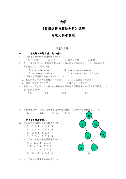
以下6-8题基于图1。
6.该二叉树结点的前序遍历的序列为( )。
A.E、G、F、A、C、D、BB.E、A、G、C、F、B、DC.E、A、C、B、D、G、FD.E、G、A、C、D、F、B7.该二叉树结点的中序遍历的序列为( )。
A. A、B、C、D、E、G、FB. E、A、G、C、F、B、DC. E、A、C、B、D、G、FE.B、D、C、A、F、G、E8.该二叉树的按层遍历的序列为( )。
A.E、G、F、A、C、D、B B. E、A、C、B、D、G、FC. E、A、G、C、F、B、DD. E、G、A、C、D、F、B9.下面关于图的存储的叙述中正确的是( )。
A.用邻接表法存储图,占用的存储空间大小只与图中边数有关,而与结点个数无关B.用邻接表法存储图,占用的存储空间大小与图中边数和结点个数都有关C. 用邻接矩阵法存储图,占用的存储空间大小与图中结点个数和边数都有关D.用邻接矩阵法存储图,占用的存储空间大小只与图中边数有关,而与结点个数无关10.设有关键码序列(q,g,m,z,a,n,p,x,h),下面哪一个序列是从上述序列出发建堆的结果?( )A. a,g,h,m,n,p,q,x,zB. a,g,m,h,q,n,p,x,zC. g,m,q,a,n,p,x,h,zD. h,g,m,p,a,n,q,x,z二、填空题(每空1分,共26分)1.数据的物理结构被分为_________、________、__________和___________四种。
《数据结构与算法分析》(C++第二版)【美】Clifford A.Shaffer著 课后习题答案 二
《数据结构与算法分析》(C++第二版)【美】Clifford A.Shaffer著课后习题答案二5Binary Trees5.1 Consider a non-full binary tree. By definition, this tree must have some internalnode X with only one non-empty child. If we modify the tree to removeX, replacing it with its child, the modified tree will have a higher fraction ofnon-empty nodes since one non-empty node and one empty node have been removed.5.2 Use as the base case the tree of one leaf node. The number of degree-2 nodesis 0, and the number of leaves is 1. Thus, the theorem holds.For the induction hypothesis, assume the theorem is true for any tree withn − 1 nodes.For the induction step, consider a tree T with n nodes. Remove from the treeany leaf node, and call the resulting tree T. By the induction hypothesis, Thas one more leaf node than it has nodes of degree 2.Now, restore the leaf node that was removed to form T. There are twopossible cases.(1) If this leaf node is the only child of its parent in T, then the number ofnodes of degree 2 has not changed, nor has the number of leaf nodes. Thus,the theorem holds.(2) If this leaf node is the child of a node in T with degree 2, then that nodehas degree 1 in T. Thus, by restoring the leaf node we are adding one newleaf node and one new node of degree 2. Thus, the theorem holds.By mathematical induction, the theorem is correct.32335.3 Base Case: For the tree of one leaf node, I = 0, E = 0, n = 0, so thetheorem holds.Induction Hypothesis: The theorem holds for the full binary tree containingn internal nodes.Induction Step: Take an arbitrary tree (call it T) of n internal nodes. Selectsome internal node x from T that has two leaves, and remove those twoleaves. Call the resulting tree T’. Tree T’ is full and has n−1 internal nodes,so by the Induction Hypothesis E = I + 2(n − 1).Call the depth of node x as d. Restore the two children of x, each at leveld+1. We have nowadded d to I since x is now once again an internal node.We have now added 2(d + 1) − d = d + 2 to E since we added the two leafnodes, but lost the contribution of x to E. Thus, if before the addition we had E = I + 2(n − 1) (by the induction hypothesis), then after the addition we have E + d = I + d + 2 + 2(n − 1) or E = I + 2n which is correct. Thus,by the principle of mathematical induction, the theorem is correct.5.4 (a) template <class Elem>void inorder(BinNode<Elem>* subroot) {if (subroot == NULL) return; // Empty, do nothingpreorder(subroot->left());visit(subroot); // Perform desired actionpreorder(subroot->right());}(b) template <class Elem>void postorder(BinNode<Elem>* subroot) {if (subroot == NULL) return; // Empty, do nothingpreorder(subroot->left());preorder(subroot->right());visit(subroot); // Perform desired action}5.5 The key is to search both subtrees, as necessary.template <class Key, class Elem, class KEComp>bool search(BinNode<Elem>* subroot, Key K);if (subroot == NULL) return false;if (subroot->value() == K) return true;if (search(subroot->right())) return true;return search(subroot->left());}34 Chap. 5 Binary Trees5.6 The key is to use a queue to store subtrees to be processed.template <class Elem>void level(BinNode<Elem>* subroot) {AQueue<BinNode<Elem>*> Q;Q.enqueue(subroot);while(!Q.isEmpty()) {BinNode<Elem>* temp;Q.dequeue(temp);if(temp != NULL) {Print(temp);Q.enqueue(temp->left());Q.enqueue(temp->right());}}}5.7 template <class Elem>int height(BinNode<Elem>* subroot) {if (subroot == NULL) return 0; // Empty subtreereturn 1 + max(height(subroot->left()),height(subroot->right()));}5.8 template <class Elem>int count(BinNode<Elem>* subroot) {if (subroot == NULL) return 0; // Empty subtreeif (subroot->isLeaf()) return 1; // A leafreturn 1 + count(subroot->left()) +count(subroot->right());}5.9 (a) Since every node stores 4 bytes of data and 12 bytes of pointers, the overhead fraction is 12/16 = 75%.(b) Since every node stores 16 bytes of data and 8 bytes of pointers, the overhead fraction is 8/24 ≈ 33%.(c) Leaf nodes store 8 bytes of data and 4 bytes of pointers; internal nodesstore 8 bytes of data and 12 bytes of pointers. Since the nodes havedifferent sizes, the total space needed for internal nodes is not the sameas for leaf nodes. Students must be careful to do the calculation correctly,taking the weighting into account. The correct formula looks asfollows, given that there are x internal nodes and x leaf nodes.4x + 12x12x + 20x= 16/32 = 50%.(d) Leaf nodes store 4 bytes of data; internal nodes store 4 bytes of pointers. The formula looks as follows, given that there are x internal nodes and35x leaf nodes:4x4x + 4x= 4/8 = 50%.5.10 If equal valued nodes were allowed to appear in either subtree, then during a search for all nodes of a given value, whenever we encounter a node of that value the search would be required to search in both directions.5.11 This tree is identical to the tree of Figure 5.20(a), except that a node with value 5 will be added as the right child of the node with value 2.5.12 This tree is identical to the tree of Figure 5.20(b), except that the value 24 replaces the value 7, and the leaf node that originally contained 24 is removed from the tree.5.13 template <class Key, class Elem, class KEComp>int smallcount(BinNode<Elem>* root, Key K);if (root == NULL) return 0;if (KEComp.gt(root->value(), K))return smallcount(root->leftchild(), K);elsereturn smallcount(root->leftchild(), K) +smallcount(root->rightchild(), K) + 1;5.14 template <class Key, class Elem, class KEComp>void printRange(BinNode<Elem>* root, int low,int high) {if (root == NULL) return;if (KEComp.lt(high, root->val()) // all to leftprintRange(root->left(), low, high);else if (KEComp.gt(low, root->val())) // all to rightprintRange(root->right(), low, high);else { // Must process both childrenprintRange(root->left(), low, high);PRINT(root->value());printRange(root->right(), low, high);}}5.15 The minimum number of elements is contained in the heap with a single node at depth h − 1, for a total of 2h−1 nodes.The maximum number of elements is contained in the heap that has completely filled up level h − 1, for a total of 2h − 1 nodes.5.16 The largest element could be at any leaf node.5.17 The corresponding array will be in the following order (equivalent to level order for the heap):12 9 10 5 4 1 8 7 3 236 Chap. 5 Binary Trees5.18 (a) The array will take on the following order:6 5 3 4 2 1The value 7 will be at the end of the array.(b) The array will take on the following order:7 4 6 3 2 1The value 5 will be at the end of the array.5.19 // Min-heap classtemplate <class Elem, class Comp> class minheap {private:Elem* Heap; // Pointer to the heap arrayint size; // Maximum size of the heapint n; // # of elements now in the heapvoid siftdown(int); // Put element in correct placepublic:minheap(Elem* h, int num, int max) // Constructor{ Heap = h; n = num; size = max; buildHeap(); }int heapsize() const // Return current size{ return n; }bool isLeaf(int pos) const // TRUE if pos a leaf{ return (pos >= n/2) && (pos < n); }int leftchild(int pos) const{ return 2*pos + 1; } // Return leftchild posint rightchild(int pos) const{ return 2*pos + 2; } // Return rightchild posint parent(int pos) const // Return parent position { return (pos-1)/2; }bool insert(const Elem&); // Insert value into heap bool removemin(Elem&); // Remove maximum value bool remove(int, Elem&); // Remove from given pos void buildHeap() // Heapify contents{ for (int i=n/2-1; i>=0; i--) siftdown(i); }};template <class Elem, class Comp>void minheap<Elem, Comp>::siftdown(int pos) { while (!isLeaf(pos)) { // Stop if pos is a leafint j = leftchild(pos); int rc = rightchild(pos);if ((rc < n) && Comp::gt(Heap[j], Heap[rc]))j = rc; // Set j to lesser child’s valueif (!Comp::gt(Heap[pos], Heap[j])) return; // Done37swap(Heap, pos, j);pos = j; // Move down}}template <class Elem, class Comp>bool minheap<Elem, Comp>::insert(const Elem& val) { if (n >= size) return false; // Heap is fullint curr = n++;Heap[curr] = val; // Start at end of heap// Now sift up until curr’s parent < currwhile ((curr!=0) &&(Comp::lt(Heap[curr], Heap[parent(curr)]))) {swap(Heap, curr, parent(curr));curr = parent(curr);}return true;}template <class Elem, class Comp>bool minheap<Elem, Comp>::removemin(Elem& it) { if (n == 0) return false; // Heap is emptyswap(Heap, 0, --n); // Swap max with last valueif (n != 0) siftdown(0); // Siftdown new root valit = Heap[n]; // Return deleted valuereturn true;}38 Chap. 5 Binary Trees// Remove value at specified positiontemplate <class Elem, class Comp>bool minheap<Elem, Comp>::remove(int pos, Elem& it) {if ((pos < 0) || (pos >= n)) return false; // Bad posswap(Heap, pos, --n); // Swap with last valuewhile ((pos != 0) &&(Comp::lt(Heap[pos], Heap[parent(pos)])))swap(Heap, pos, parent(pos)); // Push up if largesiftdown(pos); // Push down if small keyit = Heap[n];return true;}5.20 Note that this summation is similar to Equation 2.5. To solve the summation requires the shifting technique from Chapter 14, so this problem may be too advanced for many students at this time. Note that 2f(n) − f(n) = f(n),but also that:2f(n) − f(n) = n(24+48+616+ ··· +2(log n − 1)n) −n(14+28+316+ ··· +log n − 1n)logn−1i=112i− log n − 1n)= n(1 − 1n− log n − 1n)= n − log n.5.21 Here are the final codes, rather than a picture.l 00h 010i 011e 1000f 1001j 101d 11000a 1100100b 1100101c 110011g 1101k 11139The average code length is 3.234455.22 The set of sixteen characters with equal weight will create a Huffman coding tree that is complete with 16 leaf nodes all at depth 4. Thus, the average code length will be 4 bits. This is identical to the fixed length code. Thus, in this situation, the Huffman coding tree saves no space (and costs no space).5.23 (a) By the prefix property, there can be no character with codes 0, 00, or 001x where “x” stands for any binary string.(b) There must be at least one code with each form 1x, 01x, 000x where“x” could be any binary string (including the empty string).5.24 (a) Q and Z are at level 5, so any string of length n containing only Q’s and Z’s requires 5n bits.(b) O and E are at level 2, so any string of length n containing only O’s and E’s requires 2n bits.(c) The weighted average is5 ∗ 5 + 10 ∗ 4 + 35 ∗ 3 + 50 ∗ 2100bits per character5.25 This is a straightforward modification.// Build a Huffman tree from minheap h1template <class Elem>HuffTree<Elem>*buildHuff(minheap<HuffTree<Elem>*,HHCompare<Elem> >* hl) {HuffTree<Elem> *temp1, *temp2, *temp3;while(h1->heapsize() > 1) { // While at least 2 itemshl->removemin(temp1); // Pull first two treeshl->removemin(temp2); // off the heaptemp3 = new HuffTree<Elem>(temp1, temp2);hl->insert(temp3); // Put the new tree back on listdelete temp1; // Must delete the remnantsdelete temp2; // of the trees we created}return temp3;}6General Trees6.1 The following algorithm is linear on the size of the two trees. // Return TRUE iff t1 and t2 are roots of identical// general treestemplate <class Elem>bool Compare(GTNode<Elem>* t1, GTNode<Elem>* t2) { GTNode<Elem> *c1, *c2;if (((t1 == NULL) && (t2 != NULL)) ||((t2 == NULL) && (t1 != NULL)))return false;if ((t1 == NULL) && (t2 == NULL)) return true;if (t1->val() != t2->val()) return false;c1 = t1->leftmost_child();c2 = t2->leftmost_child();while(!((c1 == NULL) && (c2 == NULL))) {if (!Compare(c1, c2)) return false;if (c1 != NULL) c1 = c1->right_sibling();if (c2 != NULL) c2 = c2->right_sibling();}}6.2 The following algorithm is Θ(n2).// Return true iff t1 and t2 are roots of identical// binary treestemplate <class Elem>bool Compare2(BinNode<Elem>* t1, BinNode<Elem* t2) { BinNode<Elem> *c1, *c2;if (((t1 == NULL) && (t2 != NULL)) ||((t2 == NULL) && (t1 != NULL)))return false;if ((t1 == NULL) && (t2 == NULL)) return true;4041if (t1->val() != t2->val()) return false;if (Compare2(t1->leftchild(), t2->leftchild())if (Compare2(t1->rightchild(), t2->rightchild())return true;if (Compare2(t1->leftchild(), t2->rightchild())if (Compare2(t1->rightchild(), t2->leftchild))return true;return false;}6.3 template <class Elem> // Print, postorder traversalvoid postprint(GTNode<Elem>* subroot) {for (GTNode<Elem>* temp = subroot->leftmost_child();temp != NULL; temp = temp->right_sibling())postprint(temp);if (subroot->isLeaf()) cout << "Leaf: ";else cout << "Internal: ";cout << subroot->value() << "\n";}6.4 template <class Elem> // Count the number of nodesint gencount(GTNode<Elem>* subroot) {if (subroot == NULL) return 0int count = 1;GTNode<Elem>* temp = rt->leftmost_child();while (temp != NULL) {count += gencount(temp);temp = temp->right_sibling();}return count;}6.5 The Weighted Union Rule requires that when two parent-pointer trees are merged, the smaller one’s root becomes a child of the larger one’s root. Thus, we need to keep track of the number of nodes in a tree. To do so, modify the node array to store an integer value with each node. Initially, each node isin its own tree, so the weights for each node begin as 1. Whenever we wishto merge two trees, check the weights of the roots to determine which has more nodes. Then, add to the weight of the final root the weight of the new subtree.6.60 1 2 3 4 5 6 7 8 9 10 11 12 13 14 15-1 0 0 0 0 0 0 6 0 0 0 9 0 0 12 06.7 The resulting tree should have the following structure:42 Chap. 6 General TreesNode 0 1 2 3 4 5 6 7 8 9 10 11 12 13 14 15Parent 4 4 4 4 -1 4 4 0 0 4 9 9 9 12 9 -16.8 For eight nodes labeled 0 through 7, use the following series of equivalences: (0, 1) (2, 3) (4, 5) (6, 7) (4 6) (0, 2) (4 0)This requires checking fourteen parent pointers (two for each equivalence),but none are actually followed since these are all roots. It is possible todouble the number of parent pointers checked by choosing direct children ofroots in each case.6.9 For the “lists of Children” representation, every node stores a data value and a pointer to its list of children. Further, every child (every node except the root)has a record associated with it containing an index and a pointer. Indicatingthe size of the data value as D, the size of a pointer as P and the size of anindex as I, the overhead fraction is3P + ID + 3P + I.For the “Left Child/Right Sibling” representation, every node stores three pointers and a data value, for an overhead fraction of3PD + 3P.The first linked representation of Section 6.3.3 stores with each node a datavalue and a size field (denoted by S). Each child (every node except the root)also has a pointer pointing to it. The overhead fraction is thusS + PD + S + Pmaking it quite efficient.The second linked representation of Section 6.3.3 stores with each node adata value and a pointer to the list of children. Each child (every node exceptthe root) has two additional pointers associated with it to indicate its placeon the parent’s linked list. Thus, the overhead fraction is3PD + 3P.6.10 template <class Elem>BinNode<Elem>* convert(GTNode<Elem>* genroot) {if (genroot == NULL) return NULL;43GTNode<Elem>* gtemp = genroot->leftmost_child();btemp = new BinNode(genroot->val(), convert(gtemp),convert(genroot->right_sibling()));}6.11 • Parent(r) = (r − 1)/k if 0 < r < n.• Ith child(r) = kr + I if kr +I < n.• Left sibling(r) = r − 1 if r mod k = 1 0 < r < n.• Right sibling(r) = r + 1 if r mod k = 0 and r + 1 < n.6.12 (a) The overhead fraction is4(k + 1)4 + 4(k + 1).(b) The overhead fraction is4k16 + 4k.(c) The overhead fraction is4(k + 2)16 + 4(k + 2).(d) The overhead fraction is2k2k + 4.6.13 Base Case: The number of leaves in a non-empty tree of 0 internal nodes is (K − 1)0 + 1 = 1. Thus, the theorem is correct in the base case.Induction Hypothesis: Assume that the theorem is correct for any full Karytree containing n internal nodes.Induction Step: Add K children to an arbitrary leaf node of the tree withn internal nodes. This new tree now has 1 more internal node, and K − 1more leaf nodes, so theorem still holds. Thus, the theorem is correct, by the principle of Mathematical Induction.6.14 (a) CA/BG///FEDD///H/I//(b) CA/BG/FED/H/I6.15 X|P-----| | |C Q R---| |V M44 Chap. 6 General Trees6.16 (a) // Use a helper function with a pass-by-reference// variable to indicate current position in the// node list.template <class Elem>BinNode<Elem>* convert(char* inlist) {int curr = 0;return converthelp(inlist, curr);}// As converthelp processes the node list, curr is// incremented appropriately.template <class Elem>BinNode<Elem>* converthelp(char* inlist,int& curr) {if (inlist[curr] == ’/’) {curr++;return NULL;}BinNode<Elem>* temp = new BinNode(inlist[curr++], NULL, NULL);temp->left = converthelp(inlist, curr);temp->right = converthelp(inlist, curr);return temp;}(b) // Use a helper function with a pass-by-reference // variable to indicate current position in the// node list.template <class Elem>BinNode<Elem>* convert(char* inlist) {int curr = 0;return converthelp(inlist, curr);}// As converthelp processes the node list, curr is// incremented appropriately.template <class Elem>BinNode<Elem>* converthelp(char* inlist,int& curr) {if (inlist[curr] == ’/’) {curr++;return NULL;}BinNode<Elem>* temp =new BinNode<Elem>(inlist[curr++], NULL, NULL);if (inlist[curr] == ’\’’) return temp;45curr++ // Eat the internal node mark.temp->left = converthelp(inlist, curr);temp->right = converthelp(inlist, curr);return temp;}(c) // Use a helper function with a pass-by-reference// variable to indicate current position in the// node list.template <class Elem>GTNode<Elem>* convert(char* inlist) {int curr = 0;return converthelp(inlist, curr);}// As converthelp processes the node list, curr is// incremented appropriately.template <class Elem>GTNode<Elem>* converthelp(char* inlist,int& curr) {if (inlist[curr] == ’)’) {curr++;return NULL;}GTNode<Elem>* temp =new GTNode<Elem>(inlist[curr++]);if (curr == ’)’) {temp->insert_first(NULL);return temp;}temp->insert_first(converthelp(inlist, curr));while (curr != ’)’)temp->insert_next(converthelp(inlist, curr));curr++;return temp;}6.17 The Huffman tree is a full binary tree. To decode, we do not need to know the weights of nodes, only the letter values stored in the leaf nodes. Thus, we can use a coding much like that of Equation 6.2, storing only a bit mark for internal nodes, and a bit mark and letter value for leaf nodes.7Internal Sorting7.1 Base Case: For the list of one element, the double loop is not executed and the list is not processed. Thus, the list of one element remains unaltered and is sorted.Induction Hypothesis: Assume that the list of n elements is sorted correctlyby Insertion Sort.Induction Step: The list of n + 1 elements is processed by first sorting thetop n elements. By the induction hypothesis, this is done correctly. The final pass of the outer for loop will process the last element (call it X). This isdone by the inner for loop, which moves X up the list until a value smallerthan that of X is encountered. At this point, X has been properly insertedinto the sorted list, leaving the entire collection of n + 1 elements correctly sorted. Thus, by the principle of Mathematical Induction, the theorem is correct.7.2 void StackSort(AStack<int>& IN) {AStack<int> Temp1, Temp2;while (!IN.isEmpty()) // Transfer to another stackTemp1.push(IN.pop());IN.push(Temp1.pop()); // Put back one elementwhile (!Temp1.isEmpty()) { // Process rest of elemswhile (IN.top() > Temp1.top()) // Find elem’s placeTemp2.push(IN.pop());IN.push(Temp1.pop()); // Put the element inwhile (!Temp2.isEmpty()) // Put the rest backIN.push(Temp2.pop());}}46477.3 The revised algorithm will work correctly, and its asymptotic complexity will remain Θ(n2). However, it will do about twice as many comparisons, since it will compare adjacent elements within the portion of the list already knownto be sorted. These additional comparisons are unproductive.7.4 While binary search will find the proper place to locate the next element, it will still be necessary to move the intervening elements down one position in the array. This requires the same number of operations as a sequential search. However, it does reduce the number of element/element comparisons, and may be somewhat faster by a constant factor since shifting several elements may be more efficient than an equal number of swap operations.7.5 (a) template <class Elem, class Comp>void selsort(Elem A[], int n) { // Selection Sortfor (int i=0; i<n-1; i++) { // Select i’th recordint lowindex = i; // Remember its indexfor (int j=n-1; j>i; j--) // Find least valueif (Comp::lt(A[j], A[lowindex]))lowindex = j; // Put it in placeif (i != lowindex) // Add check for exerciseswap(A, i, lowindex);}}(b) There is unlikely to be much improvement; more likely the algorithmwill slow down. This is because the time spent checking (n times) isunlikely to save enough swaps to make up.(c) Try it and see!7.6 • Insertion Sort is stable. A swap is done only if the lower element’svalue is LESS.• Bubble Sort is stable. A swap is done only if the lower element’s valueis LESS.• Selection Sort is NOT stable. The new low value is set only if it isactually less than the previous one, but the direction of the search isfrom the bottom of the array. The algorithm will be stable if “less than”in the check becomes “less than or equal to” for selecting the low key position.• Shell Sort is NOT stable. The sublist sorts are done independently, andit is quite possible to swap an element in one sublist ahead of its equalvalue in another sublist. Once they are in the same sublist, they willretain this (incorrect) relationship.• Quick-sort is NOT stable. After selecting the pivot, it is swapped withthe last element. This action can easily put equal records out of place.48 Chap. 7 Internal Sorting• Conceptually (in particular, the linked list version) Mergesort is stable.The array implementations are NOT stable, since, given that the sublistsare stable, the merge operation will pick the element from the lower listbefore the upper list if they are equal. This is easily modified to replace“less than” with “less than or equal to.”• Heapsort is NOT stable. Elements in separate sides of the heap are processed independently, and could easily become out of relative order.• Binsort is stable. Equal values that come later are appended to the list.• Radix Sort is stable. While the processing is from bottom to top, thebins are also filled from bottom to top, preserving relative order.7.7 In the worst case, the stack can store n records. This can be cut to log n in the worst case by putting the larger partition on FIRST, followed by the smaller. Thus, the smaller will be processed first, cutting the size of the next stacked partition by at least half.7.8 Here is how I derived a permutation that will give the desired (worst-case) behavior:a b c 0 d e f g First, put 0 in pivot index (0+7/2),assign labels to the other positionsa b c g d e f 0 First swap0 b c g d e f a End of first partition pass0 b c g 1 e f a Set d = 1, it is in pivot index (1+7/2)0 b c g a e f 1 First swap0 1 c g a e f b End of partition pass0 1 c g 2 e f b Set a = 2, it is in pivot index (2+7/2)0 1 c g b e f 2 First swap0 1 2 g b e f c End of partition pass0 1 2 g b 3 f c Set e = 3, it is in pivot index (3+7/2)0 1 2 g b c f 3 First swap0 1 2 3 b c f g End of partition pass0 1 2 3 b 4 f g Set c = 4, it is in pivot index (4+7/2)0 1 2 3 b g f 4 First swap0 1 2 3 4 g f b End of partition pass0 1 2 3 4 g 5 b Set f = 5, it is in pivot index (5+7/2)0 1 2 3 4 g b 5 First swap0 1 2 3 4 5 b g End of partition pass0 1 2 3 4 5 6 g Set b = 6, it is in pivot index (6+7/2)0 1 2 3 4 5 g 6 First swap0 1 2 3 4 5 6 g End of parition pass0 1 2 3 4 5 6 7 Set g = 7.Plugging the variable assignments into the original permutation yields:492 6 4 0 13 5 77.9 (a) Each call to qsort costs Θ(i log i). Thus, the total cost isni=1i log i = Θ(n2 log n).(b) Each call to qsort costs Θ(n log n) for length(L) = n, so the totalcost is Θ(n2 log n).7.10 All that we need to do is redefine the comparison test to use strcmp. The quicksort algorithm itself need not change. This is the advantage of paramerizing the comparator.7.11 For n = 1000, n2 = 1, 000, 000, n1.5 = 1000 ∗√1000 ≈ 32, 000, andn log n ≈ 10, 000. So, the constant factor for Shellsort can be anything less than about 32 times that of Insertion Sort for Shellsort to be faster. The constant factor for Shellsort can be anything less than about 100 times thatof Insertion Sort for Quicksort to be faster.7.12 (a) The worst case occurs when all of the sublists are of size 1, except for one list of size i − k + 1. If this happens on each call to SPLITk, thenthe total cost of the algorithm will be Θ(n2).(b) In the average case, the lists are split into k sublists of roughly equal length. Thus, the total cost is Θ(n logk n).7.13 (This question comes from Rawlins.) Assume that all nuts and all bolts havea partner. We use two arrays N[1..n] and B[1..n] to represent nuts and bolts. Algorithm 1Using merge-sort to solve this problem.First, split the input into n/2 sub-lists such that each sub-list contains twonuts and two bolts. Then sort each sub-lists. We could well come up with apair of nuts that are both smaller than either of a pair of bolts. In that case,all you can know is something like:N1, N2。
数据结构与算法分析c语言描述中文答案
数据结构与算法分析c语言描述中文答案一、引言数据结构与算法是计算机科学中非常重要的基础知识,它们为解决实际问题提供了有效的工具和方法。
本文将以C语言描述中文的方式,介绍数据结构与算法分析的基本概念和原理。
二、数据结构1. 数组数组是在内存中连续存储相同类型的数据元素的集合。
在C语言中,可以通过定义数组类型、声明数组变量以及对数组进行操作来实现。
2. 链表链表是一种动态数据结构,它由一系列的节点组成,每个节点包含了数据和一个指向下一个节点的指针。
链表可以是单链表、双链表或循环链表等多种形式。
3. 栈栈是一种遵循“先进后出”(Last-In-First-Out,LIFO)原则的数据结构。
在C语言中,可以通过数组或链表实现栈,同时实现入栈和出栈操作。
4. 队列队列是一种遵循“先进先出”(First-In-First-Out,FIFO)原则的数据结构。
在C语言中,可以通过数组或链表实现队列,同时实现入队和出队操作。
5. 树树是一种非线性的数据结构,它由节点和边组成。
每个节点可以有多个子节点,其中一个节点被称为根节点。
在C语言中,可以通过定义结构体和指针的方式来实现树的表示和操作。
6. 图图是由顶点和边组成的数据结构,它可以用来表示各种实际问题,如社交网络、路网等。
在C语言中,可以通过邻接矩阵或邻接表的方式来表示图,并实现图的遍历和查找等操作。
三、算法分析1. 时间复杂度时间复杂度是用来衡量算法的执行时间随着问题规模增长的趋势。
常见的时间复杂度有O(1)、O(log n)、O(n)、O(n^2)等,其中O表示“量级”。
2. 空间复杂度空间复杂度是用来衡量算法的执行所需的额外内存空间随着问题规模增长的趋势。
常见的空间复杂度有O(1)、O(n)等。
3. 排序算法排序算法是对一组数据按照特定规则进行排序的算法。
常见的排序算法有冒泡排序、插入排序、选择排序、快速排序、归并排序等,它们的时间复杂度和空间复杂度各不相同。
数据结构经典书籍
数据结构经典书籍摘要:一、数据结构的重要性二、数据结构的经典书籍介绍1.《数据结构与算法分析》2.《大话数据结构》3.《数据结构与算法》4.《算法导论》5.《数据结构与算法之美》三、如何选择适合自己的数据结构书籍四、结论正文:数据结构是计算机科学中至关重要的一个领域,掌握数据结构有助于编写高效、可读和可维护的代码。
在众多数据结构书籍中,有几本被广泛认为是经典之作。
本文将介绍其中的五本,并讨论如何选择适合自己的数据结构书籍。
1.《数据结构与算法分析》(Data Structures and Algorithm Analysis in Java)作者:Mark Allen Weiss这本书以Java 语言为例,详细讲述了数据结构和算法的基本概念、原理和实现。
书中包含大量实例和习题,适合初学者入门。
2.《大话数据结构》作者:程云本书采用轻松幽默的语言和丰富的图解,讲解了数据结构的基本原理和常用算法。
内容通俗易懂,适合编程初学者。
3.《数据结构与算法》(Data Structures and Algorithms)作者:Alfred V.Aho, John E.Hopcroft, and Jeffrey D.Ullman这本书是数据结构和算法的经典教材,详细介绍了各种数据结构及其操作,以及排序、查找等基本算法。
内容较为深入,适合已经掌握基本编程技能的读者。
4.《算法导论》(Introduction to Algorithms)作者:Thomas H.Cormen, Charles E.Leiserson, Ronald L.Rivest, and Clifford Stein本书全面讲述了算法设计与分析的基本概念,涵盖了许多经典算法和数据结构。
书中包含大量实例和习题,适合对算法有一定了解的读者深入学习。
5.《数据结构与算法之美》(The Art of Computer Programming, Volume 1: Fundamental Algorithms)作者:Donald E.Knuth本书是计算机编程艺术的卷一,讲述了计算机科学的基本算法。
数据结构经典书籍

数据结构经典书籍数据结构是计算机科学中的一门基础课程,它研究如何组织和存储数据,以便能够高效地访问和操作。
在学习数据结构时,经典书籍是我们不可或缺的学习资料。
下面是我列举的一些经典的数据结构书籍,它们涵盖了各种不同的数据结构和算法,帮助读者深入理解和掌握数据结构的基本原理和应用。
1. 《数据结构与算法分析》这本书由Mark Allen Weiss编写,是数据结构领域的经典教材之一。
它介绍了各种常见的数据结构和算法,并提供了详细的分析和实现示例。
该书以清晰的语言和丰富的示意图,帮助读者理解不同数据结构的特点和应用场景。
2. 《算法导论》由Thomas H. Cormen等人编写的《算法导论》是计算机科学领域最具影响力的教材之一。
它包含了广泛的算法和数据结构内容,并提供了详细的证明和分析。
该书不仅适合作为教材使用,也是研究和实践中的重要参考资料。
3. 《数据结构与算法分析:C语言描述》这本书由Clifford A. Shaffer编写,以C语言为基础,介绍了数据结构和算法的基本概念和实现方法。
该书通过大量的示例代码和练习题,帮助读者巩固和应用所学知识。
4. 《算法(第4版)》由Robert Sedgewick和Kevin Wayne合著的《算法(第4版)》是一本全面介绍算法和数据结构的教材。
该书以Java语言为例,涵盖了各种经典算法和数据结构的实现和分析。
它还提供了大量的练习题和在线学习资源,帮助读者深入理解和应用所学知识。
5. 《数据结构与算法分析:Java语言描述》这本书由Mark Allen Weiss编写,以Java语言为基础,介绍了数据结构和算法的基本概念和实现方法。
它通过清晰的示例代码和详细的分析,帮助读者理解和应用不同数据结构和算法。
6. 《数据结构与算法分析:Python语言描述》由Clifford A. Shaffer编写的《数据结构与算法分析:Python语言描述》是一本以Python语言为基础的数据结构教材。
数据结构与算法分析课后习题答案
数据结构与算法分析课后习题答案【篇一:《数据结构与算法》课后习题答案】>2.3.2 判断题2.顺序存储的线性表可以按序号随机存取。
(√)4.线性表中的元素可以是各种各样的,但同一线性表中的数据元素具有相同的特性,因此属于同一数据对象。
(√)6.在线性表的链式存储结构中,逻辑上相邻的元素在物理位置上不一定相邻。
(√)8.在线性表的顺序存储结构中,插入和删除时移动元素的个数与该元素的位置有关。
(√)9.线性表的链式存储结构是用一组任意的存储单元来存储线性表中数据元素的。
(√)2.3.3 算法设计题1.设线性表存放在向量a[arrsize]的前elenum个分量中,且递增有序。
试写一算法,将x 插入到线性表的适当位置上,以保持线性表的有序性,并且分析算法的时间复杂度。
【提示】直接用题目中所给定的数据结构(顺序存储的思想是用物理上的相邻表示逻辑上的相邻,不一定将向量和表示线性表长度的变量封装成一个结构体),因为是顺序存储,分配的存储空间是固定大小的,所以首先确定是否还有存储空间,若有,则根据原线性表中元素的有序性,来确定插入元素的插入位置,后面的元素为它让出位置,(也可以从高下标端开始一边比较,一边移位)然后插入x ,最后修改表示表长的变量。
int insert (datatype a[],int *elenum,datatype x) /*设elenum为表的最大下标*/ {if (*elenum==arrsize-1) return 0; /*表已满,无法插入*/else {i=*elenum;while (i=0 a[i]x)/*边找位置边移动*/{a[i+1]=a[i];i--;}a[i+1]=x;/*找到的位置是插入位的下一位*/ (*elenum)++;return 1;/*插入成功*/}}时间复杂度为o(n)。
2.已知一顺序表a,其元素值非递减有序排列,编写一个算法删除顺序表中多余的值相同的元素。
数据结构与算法 经典书籍

数据结构与算法经典书籍数据结构与算法是计算机科学中非常重要的基础知识,对于程序员来说,掌握好数据结构与算法对于解决问题、编写高效的代码至关重要。
下面是一些经典的数据结构与算法的书籍,这些书籍涵盖了常见的数据结构和算法,可以帮助读者深入理解和应用这些知识。
1.《算法导论》(Introduction to Algorithms)这是一本经典的算法教材,由Thomas H. Cormen、Charles E. Leiserson、Ronald L. Rivest和Clifford Stein合著,被广泛认为是学习算法的权威之作。
书中详细介绍了各种常用的数据结构和算法,包括排序、查找、图算法等。
2.《数据结构与算法分析:C语言描述》(Data Structures and Algorithm Analysis in C)这本书由Mark Allen Weiss编写,通过C语言的描述介绍了各种数据结构和算法。
书中详细讲解了链表、栈、队列、树等数据结构以及排序、查找、图算法等算法。
3.《算法图解》(Grokking Algorithms)这是一本非常适合初学者的算法入门书籍,由Aditya Bhargava编写。
书中使用简洁的语言和图示,介绍了常见的算法和数据结构,包括二分查找、快速排序、广度优先搜索等。
4.《算法(第4版)》(Algorithms, 4th Edition)这本书由Robert Sedgewick和Kevin Wayne合著,是一本经典的算法教材。
书中介绍了各种算法和数据结构的设计和分析方法,包括排序、查找、图算法等。
5.《数据结构与算法分析:Java语言描述》(Data Structures and Algorithm Analysis in Java)这本书由Mark Allen Weiss编写,使用Java语言描述了各种数据结构和算法。
书中详细讲解了链表、栈、队列、树等数据结构以及排序、查找、图算法等算法。
数据结构与算法设计与分析考核试卷

8.在冒泡排序中,每一趟排序都能确定一个元素的最终位置。()
答案:______
9. Prim算法和Kruskal算法都可以用来求解最小生成树问题,但Prim算法总是从某一顶点开始,而Kruskal算法总是从某一权值最小的边开始。()
答案:______
10.在一个递归算法中,如果递归调用不是算法的最后一个操作,那么这种递归称为尾递归。()
B.邻接表适合表示稀疏图
C.邻接多重表适合表示无向图
D.邻接表和邻接多重表适合表示有向图
14.以下哪些算法属于分治算法?()
A.快速排序
B.归并排序
C.二分查找
D.动态规划
15.以下哪些情况下,动态规划比贪心算法更适合解决问题?()
A.存在重叠子问题
B.问题具有最优子结构
C.需要考虑所有可能的选择
D.问题可以通过局部最优达到全局最优
C.插入一个节点
D.查找某个节点
5.以下哪些算法可以用于解决最小生成树问题?()
A. Kruskal算法
B. Prim算法
C. Dijkstra算法
D. Bellman-Ford算法
6.以下哪些数据结构可以用来实现堆?()
A.数组
B.链表
C.栈
D.队列
7.关于图的深度优先遍历和广度优先遍历,以下哪些说法是正确的?()
________________________________
2.动态规划算法通常用于解决最优化问题,请阐述动态规划算法的三个基本要素,并给出一个动态规划问题的实例。
________________________________
________________________________
数据结构与算法分析

路径
1.
2.
3. 4. 5.
6.
在无向图G 中,若存在一个顶点序列vp ,vi1 , vi2 , …vim ,vq,使得 (vp ,vi1),(vi1 ,vi2), …,(vim ,vq )∈E(G),则称顶点序列 (vp ,vi1),(vi1 ,vi2), …,(vim ,vq )∈E(G) 为从vp到vq的一条 (Path)。 在有向图G 中,若存在一个顶点序列vp ,vi1 , vi2 , …vim ,vq,使得有 向边<vp ,vi1>, <vi1 ,vi2>, …,<vim ,vq >∈E(G),则称顶点vp路到vq有 一条有向路径(Path)。 无权图的路径长度是指此路径上边的条数。 有权图的路径长度是指路径上各边的权之和。 简单路径:若路径上各顶点vp ,vi1 , vi2 , …vim ,vq均不互相同, 则称这 样的路径为简单路径。 环:若简单路径长度大于2,且第一个顶点v1 与最后一个顶点vm 重 合, 则称这样的简单路径为回路或环。
3 0 1 0 1 6 4 2
3
0 1
4
2
3
2
6
5
4
5
G的连通分量
6
5
是连通分量吗?
无向图G
强连通
在有向图中, 若一对顶点vi和vj存在一条从vi到vj和从vj到vi的路径, 则 称vi和vj是强连通的。 若有向图中任意两个顶点都是强连通的,则称该图为强连通图。 有向图的极大强连通子图称为图的强连通分量 例:
0 1 3
2 4
无向图G1
有向图
若图G的每条边都有方向,则称G为有向图(Digraph)。 有向边(即弧)由两个顶点组成的有序对来表示,记为< 起始点,终止点y> (也可称<弧尾,弧头>)。 举例: V(G2)={0,1,2,3,4} E(G2)={<0,3>,<1,0>,<1,2>,<3,1>,<3,4>,<4,2>}
【华中科技大学】《数据结构与算法分析》(827)考试大纲
华中科技大学硕士研究生统一入学考试《数据结构与算法分析》(827)考试大纲第一部分考试说明一、考试性质数据结构与算法分析是软件学院硕士生入学选考的专业基础课之一。
考试对象为参加软件学院2008年全国硕士研究生入学考试的准考考生。
二、考试形式与试卷结构(一)答卷方式:闭卷,笔试(二)答题时间:180分钟(三)考试题型及比例术语解释15%选择填空 30%简答题30%设计及应用题 25%(四)参考书目严蔚敏,吴伟民,数据结构(C语言版),清华大学出版社,1997年4月。
第二部分考查要点(一)基本概念和术语1.数据结构的概念2.抽象数据结构类型的表示与实现3.算法,算法设计的要求,算法效率的度量,存储空间要求。
(二)线形表1.线形表的类型定义2.线形表的顺序表示和实现3.线形表的链式表示和实现(三)栈和队列1.栈的定义,表示和实现2.栈的应用:数制转换,括号匹配,行编辑,迷宫求解,表达式求值.3.栈与递归实现4.队列。
(四)串1.串的定义,表示和实现2.串的模式匹配算法(五)树和二叉树1.树的定义和基本术语2.二叉树,遍历二叉树和线索二叉树3.树和森林:存储结构,与二叉树的转换,遍历4.霍夫曼树和霍夫曼编码5.回溯法与树的遍历(六)查找1.静态查找表2.动态查找表3.哈希表(七)图1.图的定义和术语2.图的存储结构3.图的遍历4.图的连通性问题5.拓扑排序与关键路径6.最短路径(八)内部排序1.排序的概念2.插入排序3.快速排序4.选择排序:简单选择,树形选择,堆排序5.归并排序6.基数排序7.各种排序方法的比较第三部分考试样题(略)。
数据结构与算法分析

数据结构与算法分析数据结构与算法分析是计算机科学领域中最为重要的基础知识之一。
它们是计算机程序设计和软件开发的基石,对于解决实际问题具有重要的指导作用。
本文将围绕数据结构与算法分析的概念、作用以及常见的数据结构和算法进行深入探讨,以便读者对其有更全面的理解。
一、数据结构的概念数据结构是计算机科学中研究组织和存储数据的方法,它关注如何将数据按照逻辑关系组织在一起并以一定的方式存储在计算机内存中。
常见的数据结构包括数组、链表、栈、队列、树等。
不同的数据结构适用于不同类型的问题,选择合适的数据结构对于算法的效率和性能至关重要。
二、算法分析的意义算法分析是对算法的效率和性能进行评估和估算的过程。
它主要关注算法的时间复杂度和空间复杂度,这两者是衡量算法性能的重要指标。
通过对算法进行分析,我们可以选择最适合解决问题的算法,提高程序的运行效率和资源利用率。
在实际开发中,合理选择和使用算法可以减少计算机的负荷,提高系统的响应速度。
三、常见的数据结构1. 数组:数组是一种线性数据结构,它以连续的内存空间存储一组相同类型的数据。
数组的优点是可以随机访问,但缺点是插入和删除操作的效率较低。
2. 链表:链表是一种常见的动态数据结构,它由一系列节点组成,每个节点包含数据和指向下一节点的指针。
链表的优点是插入和删除操作的效率较高,但访问数据的效率较低。
3. 栈:栈是一种后进先出(LIFO)的数据结构,常用操作包括入栈和出栈。
栈通常用于实现函数调用、表达式求值以及回溯算法等。
4. 队列:队列是一种先进先出(FIFO)的数据结构,它常用操作包括入队和出队。
队列通常用于实现广度优先搜索和任务调度等。
5. 树:树是一种非线性的数据结构,它以层次结构存储数据。
常见的树包括二叉树、平衡二叉树、二叉搜索树等。
树的应用非常广泛,例如数据库索引、文件系统等。
四、常见的算法1. 排序算法:排序算法用于将一组元素按照某种规则进行排序。
常见的排序算法包括冒泡排序、选择排序、插入排序、快速排序、归并排序等。
数据结构与算法分析—期末复习题及答案
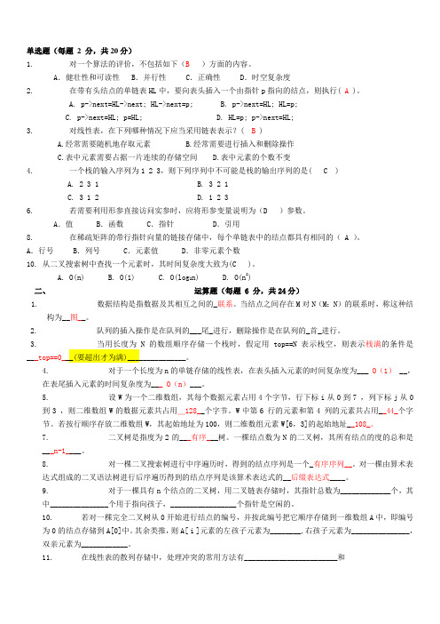
单选题(每题 2 分,共20分)1. 对一个算法的评价,不包括如下(B )方面的内容。
A.健壮性和可读性 B.并行性 C.正确性 D.时空复杂度2. 在带有头结点的单链表HL中,要向表头插入一个由指针p指向的结点,则执行( A )。
A. p->next=HL->next; HL->next=p;B. p->next=HL; HL=p;C. p->next=HL; p=HL;D. HL=p; p->next=HL;3. 对线性表,在下列哪种情况下应当采用链表表示?( B )A.经常需要随机地存取元素B.经常需要进行插入和删除操作C.表中元素需要占据一片连续的存储空间D.表中元素的个数不变4. 一个栈的输入序列为1 2 3,则下列序列中不可能是栈的输出序列的是( C )A. 2 3 1B. 3 2 1C. 3 1 2D. 1 2 36. 若需要利用形参直接访问实参时,应将形参变量说明为(D )参数。
A.值 B.函数 C.指针 D.引用8. 在稀疏矩阵的带行指针向量的链接存储中,每个单链表中的结点都具有相同的( A )。
A.行号 B.列号 C.元素值 D.非零元素个数10. 从二叉搜索树中查找一个元素时,其时间复杂度大致为(C )。
A. O(n)B. O(1)C. O(log2n)D. O(n2)二、运算题(每题 6 分,共24分)1. 数据结构是指数据及其相互之间的_联系。
当结点之间存在M对N(M:N)的联系时,称这种结构为__图__。
2. 队列的插入操作是在队列的___尾_进行,删除操作是在队列的_首_进行。
3. 当用长度为N的数组顺序存储一个栈时,假定用top==N表示栈空,则表示栈满的条件是___top==0___(要超出才为满)_______________。
4. 对于一个长度为n的单链存储的线性表,在表头插入元素的时间复杂度为___ O(1)__,在表尾插入元素的时间复杂度为___ O(n)___。
数据结构与算法分析课后习题答案

数据结构与算法分析课后习题答案第一章:基本概念一、题目:什么是数据结构与算法?数据结构是指数据在计算机中存储和组织的方式,如栈、队列、链表、树等;而算法是一系列解决问题的清晰规范的指令步骤。
数据结构和算法是计算机科学的核心内容。
二、题目:数据结构的分类有哪些?数据结构可以分为以下几类:1. 线性结构:包括线性表、栈、队列等,数据元素之间存在一对一的关系。
2. 树形结构:包括二叉树、AVL树、B树等,数据元素之间存在一对多的关系。
3. 图形结构:包括有向图、无向图等,数据元素之间存在多对多的关系。
4. 文件结构:包括顺序文件、索引文件等,是硬件和软件相结合的数据组织形式。
第二章:算法分析一、题目:什么是时间复杂度?时间复杂度是描述算法执行时间与问题规模之间的增长关系,通常用大O记法表示。
例如,O(n)表示算法的执行时间与问题规模n成正比,O(n^2)表示算法的执行时间与问题规模n的平方成正比。
二、题目:主定理是什么?主定理(Master Theorem)是用于估计分治算法时间复杂度的定理。
它的公式为:T(n) = a * T(n/b) + f(n)其中,a是子问题的个数,n/b是每个子问题的规模,f(n)表示将一个问题分解成子问题和合并子问题的所需时间。
根据主定理的不同情况,可以得到算法的时间复杂度的上界。
第三章:基本数据结构一、题目:什么是数组?数组是一种线性数据结构,它由一系列具有相同数据类型的元素组成,通过索引访问。
数组具有随机访问、连续存储等特点,但插入和删除元素的效率较低。
二、题目:栈和队列有什么区别?栈和队列都是线性数据结构,栈的特点是“先进后出”,即最后压入栈的元素最先弹出;而队列的特点是“先进先出”,即最先入队列的元素最先出队列。
第四章:高级数据结构一、题目:什么是二叉树?二叉树是一种特殊的树形结构,每个节点最多有两个子节点。
二叉树具有左子树、右子树的区分,常见的有完全二叉树、平衡二叉树等。
《数据结构与算法分析课程设计》任务书 (2)
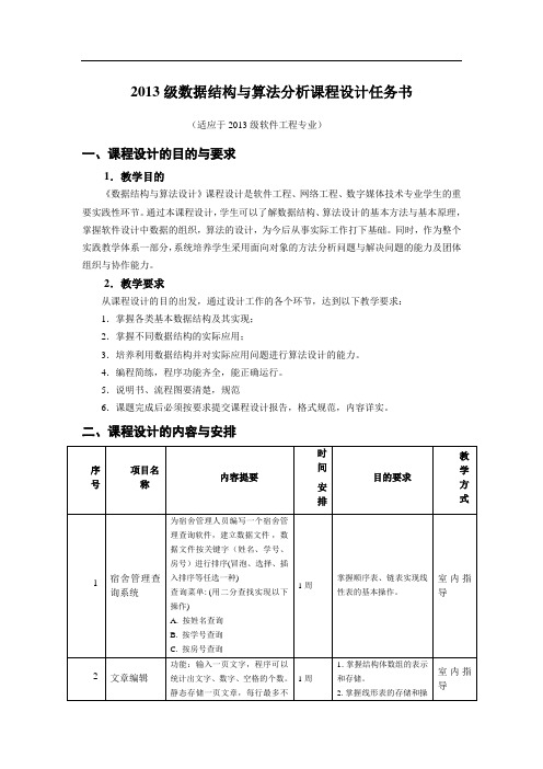
2013级数据结构与算法分析课程设计任务书(适应于2013级软件工程专业)一、课程设计的目的与要求1.教学目的《数据结构与算法设计》课程设计是软件工程、网络工程、数字媒体技术专业学生的重要实践性环节。
通过本课程设计,学生可以了解数据结构、算法设计的基本方法与基本原理,掌握软件设计中数据的组织,算法的设计,为今后从事实际工作打下基础。
同时,作为整个实践教学体系一部分,系统培养学生采用面向对象的方法分析问题与解决问题的能力及团体组织与协作能力。
2.教学要求从课程设计的目的出发,通过设计工作的各个环节,达到以下教学要求:1.掌握各类基本数据结构及其实现;2.掌握不同数据结构的实际应用;3.培养利用数据结构并对实际应用问题进行算法设计的能力。
4.编程简练,程序功能齐全,能正确运行。
5.说明书、流程图要清楚,规范6.课题完成后必须按要求提交课程设计报告,格式规范,内容详实。
二、课程设计的内容与安排注:1、鼓励各位同学自主查找资料,结合专业特性,尽量应用图形界面实现,以期对图形界面的开发有一个比较深入的了解。
2、任务要求1.问题分析和任务定义。
根据设计题目的要求,充分地分析和理解问题,明确问题要求做什么?(而不是怎么做?)限制条件是什么?2.逻辑设计。
对问题描述中涉及的操作对象定义相应的数据类型,并按照以数据结构为中心的原则划分模块,定义主程序模块和各抽象数据类型。
逻辑设计的结果应写出每个抽象数据类型的定义(包括数据结构的描述和每个基本操作的功能说明),各个主要模块的算法,并画出模块之间的调用关系图。
3.详细设计。
定义相应的存储结构并写出各函数的伪码算法。
在这个过程中,要综合考虑系统功能,使得系统结构清晰、合理、简单和易于调试,抽象数据类型的实现尽可能做到数据封装,基本操作的规格说明尽可能明确具体。
详细设计的结果是对数据结构和基本操作作出进一步的求精,写出数据存储结构的类型定义,写出函数形式的算法框架。
4.程序编码。
数据结构与算法 经典书籍

数据结构与算法经典书籍数据结构与算法是计算机科学中非常重要的一门课程,它关注如何对数据进行组织、存储和管理,以及如何设计和实现高效的算法来解决各种问题。
下面是一些经典的数据结构与算法书籍,它们涵盖了这个领域的各个方面。
1. 《算法导论》《算法导论》是由Thomas H. Cormen等人编写的一本经典教材,它详细介绍了常见的算法和数据结构,包括排序、搜索、图论等。
这本书以清晰的语言、丰富的示例和练习,帮助读者理解算法和数据结构的设计与分析。
2. 《数据结构与算法分析》《数据结构与算法分析》是由Mark Allen Weiss编写的一本经典教材,它介绍了各种数据结构和算法的设计和分析方法,包括数组、链表、树、图等。
这本书以易懂的语言和丰富的示例,帮助读者掌握数据结构与算法的基本原理和应用。
3. 《算法图解》《算法图解》是由Aditya Bhargava编写的一本简明易懂的算法入门书籍,它用图解的方式介绍了常见的算法和数据结构,包括递归、排序、搜索等。
这本书适合初学者阅读,通过图解和实例,帮助读者理解算法的基本思想和应用场景。
4. 《数据结构与算法分析——C语言描述》《数据结构与算法分析——C语言描述》是由Mark Allen Weiss编写的一本经典教材,它以C语言为例,介绍了各种数据结构和算法的设计和分析方法,包括数组、链表、树、图等。
这本书通过清晰的代码和示例,帮助读者理解数据结构与算法的实现和应用。
5. 《剑指Offer》《剑指Offer》是由何海涛编写的一本面试指南,它包含了大量经典的算法题和数据结构题,涵盖了各个领域的知识点。
这本书通过详细的解题思路和代码实现,帮助读者提升解题能力和面试技巧。
6. 《编程珠玑》《编程珠玑》是由Jon Bentley编写的一本经典教材,它介绍了计算机程序设计中的各种技巧和方法,包括数据结构的选择、算法的设计等。
这本书通过丰富的实例和案例,帮助读者培养良好的编程思维和解决问题的能力。
- 1、下载文档前请自行甄别文档内容的完整性,平台不提供额外的编辑、内容补充、找答案等附加服务。
- 2、"仅部分预览"的文档,不可在线预览部分如存在完整性等问题,可反馈申请退款(可完整预览的文档不适用该条件!)。
- 3、如文档侵犯您的权益,请联系客服反馈,我们会尽快为您处理(人工客服工作时间:9:00-18:30)。
2.掌握树和二叉树结构上的各种操作
3.学会运用树和二叉树结构求解问题 1. 设计一个程序,根据二叉树的先根序列和对称序序列创建一棵用左右指针表示的二叉树
2. 根据哈夫曼算法创建哈夫曼树,并求树中每个外部结点的编码
3. 设计一个程序,把中缀表达式转换成一棵二叉树,然后通过后序遍历计算表达式的值
订票:可以订票(订票情况可以存在一个数据文件中,结构自己设定),如果该航班已经无票,可以提供相关可选择航班;
退票:可退票,退票后修改相关数据文件;客户资料有姓名,证件号,订票数量及航班情况,订单要有编号。
修改航班信息:当航班ห้องสมุดไป่ตู้息改变可以修改航班数据文件
要求:根据以上功能说明,设计航班信息,订票信息的存储结构,设计程序完成功能;
2. 根据书中介绍的思想,设计并实现一个对简化表达式求值的系统。
3. 在计算机上模拟实现农夫过河问题的解。 文本文件检索实验 1.熟悉字符串的操作
2.学会运用字符串的操作进行文本检索和查询。 1. 根据课堂介绍设计实现KMP算法
2. 试设计一个简单的文本编辑器,使之具有对字符串的输入、输出、插入、删除、查找和替换等功能
3. 对实习的结果做比较分析。
4. 设计实现一个航班信息查询与检索系统 课程实验参考教材:
* 魏开平等编著. 数据结构辅导与实验. 清华大学出版社,2006年第1版
* 瞿有甜,《数据结构与算法分析》实验指导书,2004.9
《数据结构与算法分析》
课程设计内容体系主要内容
《数据结构课程设计》课程,可使学生深化理解书本知识,致力于用学过的理论知识和上机取得的实践经验,解决具体、复杂的实际问题,培养软件工作者所需的动手能力、独立解决问题的能力。该课程设计侧重软件设计的综合训练,包括问题分析、总体结构设计、用户界面设计、程序设计基本技能和技巧、多人合作,以至一整套软件工作规范的训练和科学作风的培养。
教学单元模块 具体教学内容 绪论 绪论部分是全书的预备知识,主要对ADL语言、数据结构与算法、算法分析基础、OOP、和C++做了简单介绍 基本数据结构 基本数据结构部分包括线性表、堆栈与队列、数组、字符串、整数集合类、树(包括AVL树、伸展树等)、图(包括网络流等问题的讨论)、散列(Hash)等 典型算法 典型算法部分主要介绍了若干典型算法的实现,并给出必要的复杂性分析和比较过程,具体包括递归、排序、查找和内存管理等 复杂数据结构 复杂数据结构部分主要包括优先级队列、不相交集合类和文件结构等 算法设计技巧 典型算法设计技巧的介绍,主要包括贪婪算法、分治算法、动态规划、回溯算法和随机化算法等 应用 应用部分是上述数据结构和典型算法的一些应用示例,具体包括事件驱动模拟、等价类、残缺棋盘和图象压缩等问题的讨论,在课时允许的情况下还会介绍摊还分析、红黑树等
散列表实验 1.熟悉散列表结构
2.掌握散列函数的生成方法,掌握常规冲突处理办法
3. 学会运用散列结构求解问题
试根据全年级学生的姓名,构造一个散列表,选择适当的散列函数和解决碰撞方法,设计并实现插入、删除和查找算法,统计碰撞发生的次数。(用拉链法解决碰撞时负载因子取2,用开地址法时取1/2)
3.试编一程序,用贪心法求解一般的着色问题。 链表应用实验 1.熟悉链表结构
2.掌握链表结构上的各种操作
3.学会运用链表结构求解问题 1.试将本章介绍的两种Josephus问题的求解过程在计算机中实现,实现时要求输出的不是整数,而是实际的人名。
2.设A与B分别为两个带有头结点的有序循环链表(所谓有序是指链接点按数据域值大小链接,本题不妨设按数据域值从小到大排列),list1和list2分别为指向两个链表的指针。请写出并在计算机上实现将这两个链表合并为一个带头结点的有序循环链表的算法。 栈与队列应用实验 1.熟悉栈和队列结构
(6)建立二叉树,层序、先序遍历( 用递归或非递归的方法都可以)**
任务:要求能够输入树的各个结点,并能够输出用不同方法遍历的遍历序列;分别建立建立二叉树存储结构的的输入函数、输出层序遍历序列的函数、输出先序遍历序列的函数;
个人总结,仅供交流
功能要求:
* 可以输入各个项目的前三名或前五名的成绩;
* 能统计各学校总分;
* 可以按学校编号、学校总分、男女团体总分排序输出;
* 可以按学校编号查询学校某个项目的情况;可以按项目编号查询取得前三或前五名的学校。
规定:输入数据形式和范围:20以内的整数(如果做得更好可以输入学校的名称,运动项目的名称)
个人总结,仅供交流
个人总结
一、 课程设计要求
学生必须仔细阅读《数据结构与算法分析》课程设计方案,认真主动完成课程设计的要求。有问题及时主动通过各种方式与教师联系沟通。
学生要发挥自主学习的能力,充分利用时间,安排好课程设计的时间计划,并在课程设计过程中不断检测自己的计划完成情况,及时的向教师汇报。
课程设计按照教学要求需要两周时间完成,两周中每天(按每周5天)至少要上3-4小时的机来调试C语言设计的程序,总共至少要上机调试程序30小时。
4. 设计实现一个完成对BST树进行插入、删除、查找操作的算法,并希望有部分同学能进一步把该算法改写为针对AVL树的相关算法 图结构实验 1.熟悉图结构
2.掌握图结构上的各种操作
3.学会运用图结构求解问题 采用两种不同的图的表示方法,实现拓扑排序和关键路径的求解过程。使用实现的算法对于下图所示的AOE网,求出各活动的可能的最早开始时间和最晚开始时间。输出整个工程的最短完成时间是多少? 哪些活动是关键活动? 说明哪项活动提高速度后能导致整个工程提前完成?分析不同存储结构对于算法效率的影响。
《数据结构与算法分析》
――课程内容体系主要内容
航班信息查询与检索实验设计 1.掌握查找与排序的各种算法
2.学会选用和设计实际问题所需的查找与排序算法 对于直接插入排序、直接选择排序、起泡排序、Shell排序、快速排序和堆排序等六种算法进行上机实习。
要求:
1. 被排序的对象由计算机随机生成,长度分别取20,100,500三种。
2. 算法中增加比较次数和移动次数的统计功能。
要求:利用单向循环链表存储结构模拟此过程,按照出列的顺序输出各个人的编号。
测试数据:m的初值为20,n=7 ,7个人的密码依次为3,1,7,2,4,7,4,首先m=6,则正确的输出是什么?
输入数据:建立输入处理输入数据,输入m的初值,n ,输入每个人的密码,建立单循环链表。
输出形式:建立一个输出函数,将正确的输出序列
输入数据的形式和范围:可以输入大写、小写的英文字母、任何数字及标点符号。
输出形式:(1)分行输出用户输入的各行字符;(2)分4行输出"全部字母数"、"数字个数"、"空格个数"、"文章总字数"(3)输出删除某一字符串后的文章;
(4)约瑟夫环(Joseph)
任务:编号是1,2,......,n的n个人按照顺时针方向围坐一圈,每个人只有一个密码(正整数)。一开始任选一个正整数作为报数上限值m,从第一个仍开始顺时针方向自1开始顺序报数,报到m时停止报数。报m的人出列,将他的密码作为新的m值,从他在顺时针方向的下一个人开始重新从1报数,如此下去,直到所有人全部出列为止。设计一个程序来求出出列顺序。
2.掌握栈和队列结构上的各种操作
3.学会运用栈和队列结构求解问题 1. 设计实现一个求解n阶Hanoi塔问题的算法
提示:将n个圆盘由A依次移到C,B作为辅助塔座。当n=1时,可以直接完成。否则,将塔座A顶上的n-1个圆盘移动到塔座B上,用塔座C作为辅助塔座;然后移第n个圆盘;最后将塔座B上的n-1个圆盘移到塔座C上,并用塔座A作为辅助塔座。
输出形式:有中文提示,各学校分数为整形
界面要求:有合理的提示,每个功能可以设立菜单,根据提示,可以完成相关的功能要求。
存储结构:学生自己根据系统功能要求自己设计,但是要求运动会的相关数据要存储在数据文件中。(数据文件的数据读写方法等相关内容在c语言程序设计的书上,请自学解决)请在最后的上交资料中指明你用到的存储结构;
(3)文章编辑**
功能:输入一页文字,程序可以统计出文字、数字、空格的个数。静态存储一页文章,每行最多不超过80个字符,共N行;
要求:(1)分别统计出其中英文字母数和空格数及整篇文章总字数;(2)统计某一字符串在文章中出现的次数,并输出该次数;(3)删除某一子串,并将后面的字符前移。(4)存储结构使用线性表,分别用几个子函数实现相应的功能;
3. 设计实现一个通用的判定回文个数问题的算法程序
稀疏矩阵和广义表实验 1.熟悉稀疏矩阵和广义表结构
2.掌握稀疏矩阵和广义表结构上的各种操作
3.学会运用稀疏矩阵和广义表结构求解问题 1. 设计实现两个普通矩阵相乘的算法
2. 实现用三元组表示法实现稀疏矩阵相加及转置算法
3. 设计实现两个N次一元多项式相加的算法程序
二、 数据结构课程设计的具体内容
本次课程设计完成如下模块(共9个模块,学生可以在其中至少挑选6个功能块完成,但有**号的模块是必须要选择的)
(1) 运动会分数统计**
任务:参加运动会有n个学校,学校编号为1......n。比赛分成m个男子项目,和w个女子项目。项目编号为男子1......m,女子m+1......m+w。不同的项目取前五名或前三名积分;取前五名的积分分别为:7、5、3、2、1,前三名的积分分别为:5、3、2;哪些取前五名或前三名由学生自己设定。(m<=20,n<=20)
(5)猴子选大王**
任务:一堆猴子都有编号,编号是1,2,3 ...m ,这群猴子(m个)按照1-m的顺序围坐一圈,从第1开始数,每数到第N个,该猴子就要离开此圈,这样依次下来,直到圈中只剩下最后一只猴子,则该猴子为大王。