《运营管理》课后习题答案(2020年7月整理).pdf
第12版运营管理习题答案
第12版运营管理习题答案1. 问题描述此习题集为第12版《运营管理》一书的习题答案总结。
本文档包含了各个章节的习题答案,旨在帮助读者更好地理解和掌握运营管理的相关概念和技术。
2. 章节习题答案总结第1章绪论1.运营管理的定义:运营管理是指组织内部通过有效地整合和协调资源和流程来生产和提供产品和服务,以满足客户需求的管理活动。
2.运营管理的目的:提高生产效率、降低成本、提高产品质量、提高客户满意度。
3.运营管理的关键要素:生产活动、物流活动、营销活动、供应商与客户。
第2章运营战略与竞争优势1.运营战略的定义:运营战略是指组织在特定环境下,为实现其目标和使命而制定的运营活动计划和行动方案。
2.竞争优势的来源:成本领先、差异化、灵活性、服务质量。
3.市场需求的变化对运营战略的影响:创新、快速响应、质量要求提高、个性化需求增加。
第3章产品设计与开发1.产品设计与开发的目的:满足市场需求、提高产品质量、降低成本。
2.产品设计与开发的过程:市场调查、概念设计、详细设计、开发与测试、产品发布。
3.产品生命周期管理的重要性:确保产品在市场上持续竞争,合理安排资源分配,提高产品的市场占有率和利润。
第4章设计与管理物流系统1.物流系统的定义:物流系统是指实现物流流程中物资、信息和金钱的流动,并为组织内外部客户提供有关物流活动的管理系统。
2.物流系统的主要活动:运输、仓储、库存管理、订单处理、信息处理。
3.物流系统的设计原则:流程简化、资源统一、信息共享、风险控制。
第5章质量管理1.质量管理的定义:质量管理是指通过制定和实施一系列的管理活动,以提高产品和服务的质量、满足客户需求的管理过程。
2.质量管理的工具:质量控制图、散点图、直方图、因果图、帕累托图、流程图等。
3.质量成本的分类:预防成本、评估成本、内部失败成本、外部失败成本。
第6章运营系统的布局与设计1.运营系统布局与设计的目的:提高资源利用率、降低库存成本、减少物料搬运。
运营管理的课后习题答案
运营管理的课后习题答案运营管理的课后习题答案运营管理是一门涉及企业内部运作和资源管理的学科,它涵盖了生产、供应链、质量管理、项目管理等多个方面。
在学习运营管理的过程中,习题是一个重要的学习工具,通过解答习题可以加深对知识点的理解和应用。
下面将为大家提供一些运营管理课后习题的答案,希望对大家的学习有所帮助。
1. 生产计划是什么?它的目的是什么?答:生产计划是指根据市场需求和企业资源情况,制定生产计划的过程。
其目的是合理安排生产资源,确保按时交付产品,满足市场需求。
2. 什么是供应链管理?它的主要目标是什么?答:供应链管理是指协调和管理企业内外各个环节的活动,以实现产品或服务的顺畅流动的过程。
其主要目标是最大程度地提高供应链的效率和灵活性,减少库存和成本,提高客户满意度。
3. 什么是质量管理?它的核心原则是什么?答:质量管理是指通过制定和实施一系列质量控制措施,以确保产品或服务符合质量要求的管理过程。
其核心原则是不断追求卓越的质量,通过持续改进和员工参与,提高产品或服务的质量水平。
4. 项目管理中的关键要素有哪些?答:项目管理中的关键要素包括项目目标、项目计划、项目团队、项目资源、项目风险等。
其中,项目目标是项目的核心,项目计划是实现目标的路线图,项目团队是实施计划的关键,项目资源是支撑项目实施的基础,项目风险是需要预防和应对的不确定因素。
5. 什么是供应商评估?为什么要进行供应商评估?答:供应商评估是对供应商进行综合评价和筛选的过程。
其目的是确保选择到合适的供应商,以保证采购的品质和效益。
供应商评估可以帮助企业降低采购风险,提高供应链的稳定性和效率。
6. 什么是成本管理?成本管理的方法有哪些?答:成本管理是指对企业生产和运营过程中产生的各项成本进行有效控制和管理的过程。
成本管理的方法包括成本核算、成本控制和成本分析等。
成本核算是对成本进行分类和计算,成本控制是设定成本目标并采取措施控制成本,成本分析是对成本进行比较和分析,找出成本的优化方向。
《运营管理》课后习题答案
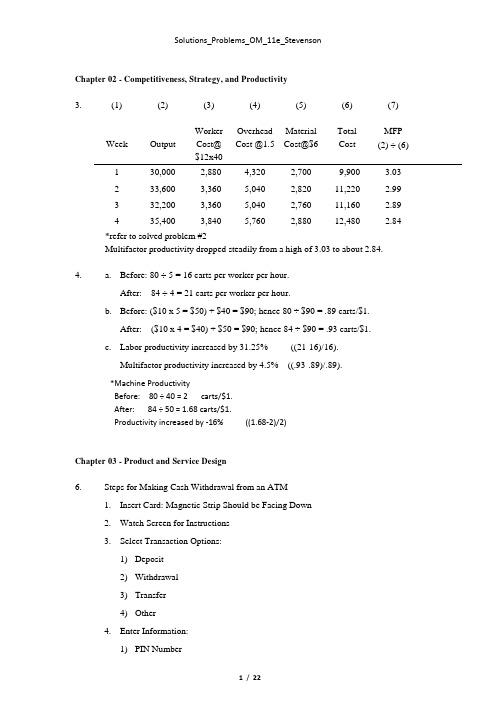
Chapter 02 - Competitiveness, Strategy, and Productivity3. (1) (2) (3) (4) (5) (6) (7)Week Output WorkerCost@$12x40Overhead********MaterialCost@$6TotalCostMFP(2) ÷ (6)1 30,000 2,880 4,320 2,700 9,900 3.032 33,600 3,360 5,040 2,820 11,220 2.993 32,200 3,360 5,040 2,760 11,160 2.894 35,400 3,840 5,760 2,880 12,480 2.84*refer to solved problem #2Multifactor productivity dropped steadily from a high of 3.03 to about 2.84.4. a. Before: 80 ÷ 5 = 16 carts per worker per hour.After: 84 ÷ 4 = 21 carts per worker per hour.b. Before: ($10 x 5 = $50) + $40 = $90; hence 80 ÷ $90 = .89 carts/$1.After: ($10 x 4 = $40) + $50 = $90; hence 84 ÷ $90 = .93 carts/$1.c. Labor productivity increased by 31.25% ((21-16)/16).Multifactor productivity increased by 4.5% ((.93-.89)/.89).*Machine ProductivityBefore: 80 ÷ 40 = 2 carts/$1.After: 84 ÷ 50 = 1.68 carts/$1.Productivity increased by -16% ((1.68-2)/2)Chapter 03 - Product and Service Design6. Steps for Making Cash Withdrawal from an ATM1. Insert Card: Magnetic Strip Should be Facing Down2. Watch Screen for Instructions3. Select Transaction Options:1) Deposit2) Withdrawal3) Transfer4) Other4. Enter Information:1) PIN Number2) Select a Transaction and Account3) Enter Amount of Transaction5. Deposit/Withdrawal: 1) Deposit —place in an envelop e (which you’ll find near or in the ATM) andinsert it into the deposit slot2) Withdrawal —lift the “Withdrawal Door,” being careful to remove all cash6. Remove card and receipt (which serves as the transaction record)8.Chapter 04 - Strategic Capacity Planning for Products and Services2. %80capacityEffective outputActual Efficiency ==Actual output = .8 (Effective capacity) Effective capacity = .5 (Design capacity) Actual output = (.5)(.8)(Effective capacity) Actual output = (.4)(Design capacity) Actual output = 8 jobs Utilization = .4capacityDesign outputActual =n Utilizatiojobs 204.8capacity Effective output Actual Capacity Design ===10. a. Given: 10 hrs. or 600 min. of operating time per day.250 days x 600 min. = 150,000 min. per year operating time.Total processing time by machineProductABC 1 48,000 64,000 32,000 2 48,000 48,000 36,000 3 30,000 36,000 24,000 460,000 60,000 30,000 Total 186,000208,000122,000machine181.000,150000,122machine 238.1000,150000,208machine224.1000,150000,186≈==≈==≈==C B A N N NYou would have to buy two “A” machines at a total cost of $80,000, or two “B” machines at a total cost of $60,000, or one “C” machine at $80,000.b.Total cost for each type of machine:A (2): 186,000 min ÷ 60 = 3,100 hrs. x $10 = $31,000 + $80,000 = $111,000B (2) : 208,000 ÷ 60 = 3,466.67 hrs. x $11 = $38,133 + $60,000 = $98,133 C(1): 122,000 ÷ 60 = 2,033.33 hrs. x $12 = $24,400 + $80,000 = $104,400Buy 2 Bs —these have the lowest total cost.Chapter 05 - Process Selection and Facility Layout3.Desired output = 4Operating time = 56 minutesunit per minutes 14hourper units 4hourper minutes 65output Desired time Operating CT ===Task # of Following tasksPositional WeightA 4 23B 3 20C 2 18D 3 25E 2 18F 4 29G 3 24H 1 14 I5a. First rule: most followers. Second rule: largest positional weight.Assembly Line Balancing Table (CT = 14)b. First rule: Largest positional weight.Assembly Line Balancing Table (CT = 14)c. %36.805645stations of no. x CT time Total Efficiency ===4. a. l.2. Minimum Ct = 1.3 minutesTask Following tasksa 4b 3c 3d 2e 3f 2g 1h3. percent 54.11)3.1(46.CT x N time)(idle percent Idle ==∑=4. 420 min./day 323.1 ( 323)/1.3 min./OT Output rounds to copiers day CT cycle=== b. 1. inutes m 3.224.6N time Total CT ,6.4 time Total ==== 2. Assign a, b, c, d, and e to station 1: 2.3 minutes [no idle time]Assign f, g, and h to station 2: 2.3 minutes3. 420182.6 copiers /2.3OT Output day CT ===4.420 min./dayMaximum Ct is 4.6. Output 91.30 copiers /4.6 min./day cycle==7.Chapter 06 - Work Design and Measurement3. Element PR OT NT AF job ST1 .90.46.414 1.15 .4762 .85 1.505 1.280 1.15 1.4723 1.10.83.913 1.15 1.05041.00 1.16 1.160 1.15 1.334Total4.3328. A = 24 + 10 + 14 = 48 minutes per 4 hours.min 125.720.11x70.5ST .min 70.5)95(.6NT 20.24048A =-=====9. a. Element PR OT NT A ST1 1.10 1.19 1.309 1.15 1.5052 1.15 .83 .955 1.15 1.09831.05.56.588 1.15 .676b.01.A 00.2z 034.s 83.x ==== 222(.034)67.12~68.01(.83)zs n observations ax ⎛⎫⎛⎫===⎪ ⎪⎝⎭⎝⎭c. e = .01 minutes 47 to round ,24.4601.)034(.2e zs n 22=⎪⎭⎫⎝⎛=⎪⎭⎫ ⎝⎛=Chapter 07- Location Planning and Analysis1. Factor Local bank Steel mill Food warehouse Public school1. Convenience forcustomers H L M–H M–H2. Attractiveness ofbuilding H L M M–H3. Nearness to rawmaterials L H L M4. Large amounts ofpower L H L L5. Pollution controls L H L L6. Labor cost andavailability L M L L7. Transportationcosts L M–H M–H M8. Constructioncosts M H M M–HLocation (a) Location (b)4. Factor A B C Weight A B C1. Business Services 9 5 5 2/9 18/9 10/9 10/92. Community Services 7 6 7 1/9 7/9 6/9 7/93. Real Estate Cost 3 8 7 1/9 3/9 8/9 7/94. Construction Costs 5 6 5 2/9 10/9 12/9 10/95. Cost of Living 4 7 8 1/9 4/9 7/9 8/96. Taxes 5 5 5 1/9 5/9 5/9 4/97. Transportation 6 7 8 1/9 6/9 7/9 8/9Total 39 44 45 1.0 53/9 55/9 54/9 Each factor has a weight of 1/7.a. Composite Scores 39 44 45 7 7 7B orC is the best and A is least desirable.b. Business Services and Construction Costs both have a weight of 2/9; the other factors eachhave a weight of 1/9.5 x + 2 x + 2 x = 1 x = 1/9c. Composite ScoresA B C 53/9 55/9 54/9B is the best followed byC and then A.5.Locationx yA 3 7B 8 2C 4 6D 4 1E 6 4Totals 25 20-x =∑x i= 25 = 5.0 -y =∑y i= 20 = 4.0 n 5 n 5Hence, the center of gravity is at (5,4) and therefore the optimal location.Chapter 08 - Management of Quality1. ChecksheetWork Type FrequencyLube and Oil 12Brakes 7Tires 6Battery 4Transmission 1Total 30ParetoLube & Oil Brakes Tires Battery Trans.2 .The run charts seems to show a pattern of errors possibly linked to break times or the end of the shift. Perhaps workers are becoming fatigued. If so, perhaps two 10 minute breaks in the morning and again in the afternoon instead of one 20 minute break could reduce some errors. Also, errors are occurring during the last few minutes before noon and the end of the shift, and those periods should also be given management’s attention.4break lunch break3 2 1 0• • •• • • ••• • • ••••••• ••• •• • •• • •••Chapter 9 - Quality Control4. Sample Mean Range179.48 2.6 Mean Chart: =X ± A 2-R = 79.96 ± 0.58(1.87) 2 80.14 2.3 = 79.96 ± 1.083 80.14 1.2UCL = 81.04, LCL = 78.884 79.60 1.7 Range Chart: UCL = D 4-R = 2.11(1.87) = 3.95 5 80.02 2.0LCL = D 3-R = 0(1.87) = 0680.381.4[Both charts suggest the process is in control: Neither has any points outside the limits.]6. n = 200 Control Limits = np p p )1(2-±Thus, UCL is .0234 and LCL becomes 0.Since n = 200, the fraction represented by each data point is half the amount shown. E.g., 1 defective = .005, 2 defectives = .01, etc.Sample 10 is too large.7. 857.714110c ==Control limits: 409.8857.7c 3c ±=± UCL is 16.266, LCL becomes 0.All values are within the limits.14. Let USL = Upper Specification Limit, LSL = Lower Specification Limit,X = Process mean, σ = Process standard deviationFor process H:}{capablenot ,0.193.93.04.1 ,938.min 04.1)32)(.3(1516393.)32)(.3(1.14153<===-=σ-=-=σ-pk C X USL LSL X 0096.)200(1325==p 0138.0096.200)9904(.0096.20096.±=±=For process K:.1}17.1,0.1min{17.1)1)(3(335.3630.1)1)(3(30333===-=σ-=-=σ- C X USL LSL X pk Assuming the minimum acceptable pk C is 1.33, since 1.0 < 1.33, the process is not capable.For process T:33.1}33.1,67.1min{33.1)4.0)(3(5.181.20367.1)4.0)(3(5.165.183===-=σ-=-=σ- C X USL LSL X pk Since 1.33 = 1.33, the process is capable.Chapter 10 - Aggregate Planning and Master Scheduling7. a.No backlogs are allowedPeriodForecast Output Regular Overtime Subcontract Output - Forecast Inventory Beginning Ending Average Backlog Costs: Regular Overtime Subcontract Inventory Totalb. Level strategyPeriodForecastOutputRegularOvertimeSubcontractOutput - ForecastInventoryBeginningEndingAverageBacklogCosts:RegularOvertimeSubcontractInventoryBacklogTotal8.PeriodForecastOutputRegularOvertimeSubcontractOutput- ForecastInventoryBeginningEndingAverageBacklogCosts:RegularOvertimeSubcontractInventoryBacklogTotalChapter 11 - MRP and ERP1. a. F: 2 G: 1 H: 1J: 2 x 2 = 4 L: 1 x 2 = 2 A: 1 x 4 = 4D: 2 x 4 = 8 J: 1 x 2 = 2 D: 1 x 2 = 2Totals: F = 2; G = 1; H = 1; J = 6; D = 10; L = 2; A = 44. Master Schedule10. Week 1 2 3 4Material 40 80 60 70Week 1 2 3 4Labor hr. 160 320 240 280Mach. hr. 120 240 180 210a. Capacity utilizationWeek 1 2 3 4Labor 53.3% 106.7% 80% 93.3%Machine 60% 120% 90% 105%b. C apacity utilization exceeds 100% for both labor and machine in week 2, and formachine alone in week 4.Production could be shifted to earlier or later weeks in which capacity isunderutilized. Shifting to an earlier week would result in added carrying costs;shifting to later weeks would mean backorder costs.Another option would be to work overtime. Labor cost would increase due toovertime premium, a probable decrease in productivity, and possible increase inaccidents.Chapter 12 - Inventory Management2. The following table contains figures on the monthly volume and unit costs for a random sample of 16 items for a list of 2,000 inventory items.a. See table.b. To allocate control efforts.c. It might be important for some reason other than dollar usage, such as cost of astockout, usage highly correlated to an A item, etc.3. D = 1,215 bags/yr. S = $10 H = $75a. bags HDS Q 187510)215,1(22===b. Q/2 = 18/2 = 9 bagsc.orders ordersbags bags Q D 5.67/ 18 215,1== d . S QD H 2/Q TC +=350,1$675675)10(18215,1)75(218=+=+=e. Assuming that holding cost per bag increases by $9/bag/yearQ ==84)10)(215,1(217 bags71.428,1$71.714714)10(17215,1)84(217=+=+=TCIncrease by [$1,428.71 – $1,350] = $78.714.D = 40/day x 260 days/yr. = 10,400 packagesS = $60 H = $30a. oxes b 20496.2033060)400,10(2H DS 2Q 0====b. S QD H 2Q TC +=82.118,6$82.058,3060,3)60(204400,10)30(2204=+=+=c. Yesd. )60(200400,10)30(2200TC 200+=TC 200 = 3,000 + 3,120 = $6,1206,120 – 6,118.82 (only $1.18 higher than with EOQ, so 200 is acceptable.)7.H = $2/month S = $55D 1 = 100/month (months 1–6)D 2 = 150/month (months 7–12)a. 16.74255)100(2Q :D H DS2Q 010===83.90255)150(2Q :D 02==b. The EOQ model requires this.c. Discount of $10/order is equivalent to S – 10 = $45 (revised ordering cost)1–6 TC74 = $148.32180$)45(150100)2(2150TC 145$)45(100100)2(2100TC *140$)45(50100)2(250TC 15010050=+==+==+=7–12 TC 91 =$181.66195$)45(150150)2(2150TC *5.167$)45(100150)2(2100TC 185$)45(50150)2(250TC 15010050=+==+==+=10. p = 50/ton/day u = 20 tons/day200 days/yr.S = $100 H = $5/ton per yr.a. bags] [10,328 tons 40.5162050505100)000,4(2u p p H DS 2Q 0=-=-=b. ]bags 8.196,6 .approx [ tons 84.309)30(504.516)u p (P Q I max ==-=Average is92.154248.309:2I max =tons [approx. 3,098 bags] c. Run length =days 33.10504.516P Q == d. Runs per year = 8] approx .[ 7.754.516000,4QD == e. Q ' = 258.2TC =S QD H 2I max + TC orig. = $1,549.00 TC rev. = $ 774.50Savings would be $774.50D= 20 tons/day x 200 days/yr. = 4,000 tons/yr.15. RangeP H Q D = 4,900 seats/yr. 0–999 $5.00 $2.00 495 H = .4P 1,000–3,999 4.95 1.98 497 NF S = $50 4,000–5,999 4.90 1.96 500 NF 6,000+ 4.85 1.94503 NFCompare TC 495 with TC for all lower price breaks:TC 495 =495 ($2) + 4,900($50) + $5.00(4,900) = $25,490 2 495 TC 1,000 = 1,000 ($1.98) + 4,900($50) + $4.95(4,900) = $25,4902 1,000 TC 4,000 = 4,000 ($1.96) + 4,900($50) + $4.90(4,900) = $27,9912 4,000 TC 6,000 = 6,000 ($1.94) + 4,900($50) + $4.85(4,900) = $29,6262 6,000Hence, one would be indifferent between 495 or 1,000 units 22. d = 30 gal./day ROP = 170 gal. LT = 4 days,ss = Z σd LT = 50 galRisk = 9% Z = 1.34 Solving, σd LT = 37.31 3% Z = 1.88, ss=1.88 x 37.31 = 70.14 gal.Chapter 13 - JIT and Lean Operations1. N = ?N = DT(1 + X)D = 80 pieces per hourC T = 75 min. = 1.25 hr. = 80(1.25) (1.35)= 3C = 45 45X = .35QuantityTC4. The smallest daily quantity evenly divisible into all four quantities is 3. Therefore, usethree cycles.Product Daily quantity Units per cycleA 21 21/3 = 7B 12 12/3 = 4C 3 3/3 = 1D 15 15/3 = 55.a. Cycle 1 2 3 4A 6 6 5 5B 3 3 3 3C 1 1 1 1D 4 4 5 5E 2 2 2 2 b. Cycle 1 2A 11 11B 6 6C 2 2D 8 8E 4 4c. 4 cycles = lower inventory, more flexibility2 cycles = fewer changeovers7. Net available time = 480 – 75 = 405. Takt time = 405/300 units per day = 1.35 minutes. Chapter 15 - Scheduling6. a. FCFS: A–B–C–DSPT: D–C–B–AEDD: C–B–D–ACR: A–C–D–BFCFS: Job time Flow time Due date DaysJob (days) (days) (days) tardyA 14 14 20 0B 10 24 16 8C 7 31 15 16D 6 37 17 2037 106 44SPT: Job time Flow time Due date Days Job (days) (days) (days) tardyD 6 6 17 0C 7 13 15 0B 10 23 16 7A 14 37 20 1737 79 24EDD:Job D has the lowest critical ratio therefore it is scheduled next and completed on day 27.b.ardi Flow time Average flow time Number of jobsDays tardy Average job t ness Number of jobs Flow timeAverage number of jobs at the center Makespan==∑=FCFS SPT EDD CR26.50 19.75 21.00 24.75 11.0 6.00 6.00 9.25 2.86 2.142.272.67c. SPT is superior.9.Thus, the sequence is b-a-g-e-f-d-c.。
智慧树运营管理课后答案
智慧树运营管理课后答案1. 简介本文是智慧树课程《运营管理》的课后答案。
运营管理是管理学的重要分支,旨在帮助企业有效组织、规划和控制生产过程,以提高生产效率并提供高质量的产品和服务。
2. 课后答案以下是智慧树课程《运营管理》中各章节的课后答案:第一章:运营管理导论1.运营管理是指企业对生产系统和分销系统进行规划、组织、实施和控制的管理活动。
2.运营管理的目标是提高生产效率、提供高质量的产品和服务、降低成本并满足顾客需求。
3.运营管理的主要职能包括生产计划和控制、库存管理、供应链管理、质量管理等。
第二章:产品和服务设计1.产品设计是指确定产品的功能、特性和性能,并为其提供合适的外观和包装。
2.服务设计是指确定服务的特性、流程和交付方式,并为其提供合适的服务环境和设施。
3.产品和服务设计的目标是满足顾客需求、提高产品价值和降低生产成本。
第三章:过程设计和分析1.过程设计是指确定产品或服务的生产流程和操作步骤。
2.过程分析是指研究和改进生产过程,以提高生产效率和质量。
3.过程设计和分析的工具和技术包括流程图、价值流图、工艺分析和工作测量等。
第四章:物料管理和供应链管理1.物料管理是指对物料的采购、储存和使用进行有效管理。
2.供应链管理是指对供应商、生产商和分销商之间的物流、信息流和资金流进行协调和管理。
3.物料管理和供应链管理的目标是降低成本、提高响应速度和提供优质的产品和服务。
第五章:质量管理和绩效评价1.质量管理是指通过一系列控制和改进措施,确保产品和服务的质量符合顾客的要求和期望。
2.绩效评价是指对企业运营绩效进行量化和评估,以判断是否达到预期目标。
3.质量管理和绩效评价的工具和技术包括质量控制图、质量成本、平衡计分卡等。
3. 总结本文总结了智慧树课程《运营管理》中各章节的课后答案。
通过学习运营管理,我们可以了解企业如何通过有效组织、规划和控制生产过程,提高生产效率、降低成本并提供高质量的产品和服务。
运营管理课后习题答案

Chapter 02 - Competitiveness, Strategy, and Productivity3. (1) (2) (3) (4) (5) (6) (7)Week Output WorkerCost@$12x40OverheadCost @MaterialCost@$6TotalCostMFP(2) ÷ (6)1 30,000 2,880 4,320 2,700 9,9002 33,600 3,360 5,040 2,820 11,2203 32,200 3,360 5,040 2,760 11,1604 35,400 3,840 5,760 2,880 12,480*refer to solved problem #2Multifactor productivity dropped steadily from a high of to about .4. a. Before: 80 ÷ 5 = 16 carts per worker per hour.After: 84 ÷ 4 = 21 carts per worker per hour.b. Before: ($10 x 5 = $50) + $40 = $90; hence 80 ÷ $90 = .89 carts/$1.After: ($10 x 4 = $40) + $50 = $90; hence 84 ÷ $90 = .93 carts/$1.c. Labor productivity increased by % ((21-16)/16).Multifactor productivity increased by % ((./.89).*Machine ProductivityBefore: 80 ÷ 40 = 2 carts/$1.After: 84 ÷ 50 = carts/$1.Productivity increased by -16% (/2)Chapter 03 - Product and Service Design6. Steps for Making Cash Withdrawal from an ATM1. Insert Card: Magnetic Strip Should be Facing Down2. Watch Screen for Instructions3. Select Transaction Options:1) Deposit2) Withdrawal3) Transfer4) Other4. Enter Information:1) PIN Number2) Select a Transaction and Account3) Enter Amount of Transaction5. Deposit/Withdrawal: 1) Deposit —place in an envelope (which you’ll find near or in the ATM) andinsert it into the deposit slot2) Withdrawal —lift the “Withdrawal Door,” being careful to remove all cash6. Remove card and receipt (which serves as the transaction record)8.Chapter 04 - Strategic Capacity Planning for Products and Services2. %80capacityEffective outputActual Efficiency ==Actual output = .8 (Effective capacity) Effective capacity = .5 (Design capacity) Actual output = (.5)(.8)(Effective capacity) Actual output = (.4)(Design capacity) Actual output = 8 jobs Utilization = .4capacityDesign outputActual =n Utilizatiojobs 204.8capacity Effective output Actual Capacity Design ===10. a. Given: 10 hrs. or 600 min. of operating time per day.250 days x 600 min. = 150,000 min. per year operating time.Total processing time by machineProductABC 1 48,000 64,000 32,000 2 48,000 48,000 36,000 3 30,000 36,000 24,000 460,000 60,000 30,000 Total 186,000208,000122,000machine181.000,150000,122machine 238.1000,150000,208machine224.1000,150000,186≈==≈==≈==C B A N N NYou would have to buy two “A” machines at a total cost of $80,000, or two “B” machines at a total cost of $60,000, or one “C” machine at $80,000.b.Total cost for each type of machine:A (2): 186,000 min ÷ 60 = 3,100 hrs. x $10 = $31,000 + $80,000 = $111,000B (2) : 208,000 ÷ 60 = 3, hrs. x $11 = $38,133 + $60,000 = $98,133 C(1): 122,000 ÷ 60 = 2, hrs. x $12 = $24,400 + $80,000 = $104,400Buy 2 Bs —these have the lowest total cost.Chapter 05 - Process Selection and Facility Layout3.Desired output = 4Operating time = 56 minutesunit per minutes 14hourper units 4hourper minutes 65output Desired time Operating CT ===Task # of Following tasksPositional WeightA 4 23B 3 20C 2 18D 3 25E 2 18F 4 29G 3 24H 1 14 I5a. First rule: most followers. Second rule: largest positional weight.Assembly Line Balancing Table (CT = 14)b. First rule: Largest positional weight.Assembly Line Balancing Table (CT = 14)c. %36.805645stations of no. x CT time Total Efficiency ===4. a. l.2. Minimum Ct = minutesTask Following tasksa 4b 3c 3d 2e 3f 2g 1h3. percent 54.11)3.1(46.CT x N time)(idle percent Idle ==∑=4. 420 min./day 323.1 ( 323)/1.3 min./OT Output rounds to copiers day CT cycle=== b. 1. inutes m 3.224.6N time Total CT ,6.4 time Total ==== 2. Assign a, b, c, d, and e to station 1: minutes [no idle time]Assign f, g, and h to station 2: minutes3. 420182.6 copiers /2.3OT Output day CT ===4.420 min./dayMaximum Ct is 4.6. Output 91.30 copiers /4.6 min./day cycle==7.Chapter 06 - Work Design and Measurement3. Element PR OT NT AF jobST1 .90 .46 .414 .4762 .853 .83 .913 4Total8. A = 24 + 10 + 14 = 48 minutes per 4 hours.min 125.720.11x70.5ST .min 70.5)95(.6NT 20.24048A =-=====9. a. Element PR OT NT A ST12 .83 .9553.56.588.676b.01.A 00.2z 034.s 83.x ==== 222(.034)67.12~68.01(.83)zs n observations ax ⎛⎫⎛⎫===⎪ ⎪⎝⎭⎝⎭c. e = .01 minutes 47 to round ,24.4601.)034(.2e zs n 22=⎪⎭⎫⎝⎛=⎪⎭⎫ ⎝⎛=Chapter 07- Location Planning and Analysis1. Factor Local bank Steel mill Food warehouse Public school1. Convenience forcustomers H L M–H M–H2. Attractiveness ofbuilding H L M M–H3. Nearness to rawmaterials L H L M4. Large amounts ofpower L H L L5. Pollution controls L H L L6. Labor cost andavailability L M L L7. Transportationcosts L M–H M–H M8. Constructioncosts M H M M–HLocation (a) Location (b)4. Factor A B C Weight A B C1. Business Services 9 5 5 2/9 18/9 10/9 10/92. Community Services 7 6 7 1/9 7/9 6/9 7/93. Real Estate Cost 3 8 7 1/9 3/9 8/9 7/94. Construction Costs 5 6 5 2/9 10/9 12/9 10/95. Cost of Living 4 7 8 1/9 4/9 7/9 8/96. Taxes 5 5 5 1/9 5/9 5/9 4/97. Transportation 6 7 8 1/9 6/9 7/9 8/9Total 39 44 45 53/9 55/9 54/9 Each factor has a weight of 1/7.a. Composite Scores 39 44 45 7 7 7B orC is the best and A is least desirable.b. Business Services and Construction Costs both have a weight of 2/9; the other factors eachhave a weight of 1/9.5 x + 2 x + 2 x = 1 x = 1/9c. Composite ScoresA B C 53/9 55/9 54/9B is the best followed byC and then A.5.Locationx yA 3 7B 8 2C 4 6D 4 1E 6 4Totals 25 20-x =∑x i= 25 = -y =∑y i= 20 = n 5 n 5Hence, the center of gravity is at (5,4) and therefore the optimal location.Chapter 08 - Management of Quality1. ChecksheetWork Type FrequencyLube and Oil 12Brakes 7Tires 6Battery 4Transmission 1Total 30ParetoLube & Oil Brakes Tires Battery Trans.2 .The run charts seems to show a pattern of errors possibly linked to break times or the end of the shift. Perhaps workers are becoming fatigued. If so, perhaps two 10 minute breaks in the morning and again in the afternoon instead of one 20 minute break could reduce some errors. Also, errors are occurring during the last few minutes before noon and the end of the shift, and those periods should also be given management’s attention.4break lunch break3 2 1 0• • •• • • ••• • • ••••••• ••• •• • •• • •••Chapter 9 - Quality Control4. Sample Mean Range1Mean Chart: =X ± A 2-R = ± 2 = ±3UCL = , LCL =4 Range Chart: UCL = D 4-R = = 5LCL = D 3-R = 0 = 06[Both charts suggest the process is in control: Neither has any points outside the limits.]6. n = 200 Control Limits = np p p )1(2-±Thus, UCL is .0234 and LCL becomes 0.Since n = 200, the fraction represented by each data point is half the amount shown. ., 1 defective = .005, 2 defectives = .01, etc.Sample 10 is too large.7. 857.714110c ==Control limits: 409.8857.7c 3c ±=± UCL is , LCL becomes 0.All values are within the limits.14. Let USL = Upper Specification Limit, LSL = Lower Specification Limit,X = Process mean, σ = Process standard deviationFor process H:}{capablenot ,0.193.93.04.1 ,938.min 04.1)32)(.3(1516393.)32)(.3(1.14153<===-=σ-=-=σ-pk C X USL LSL X 0096.)200(1325==p 0138.0096.200)9904(.0096.20096.±=±=For process K:.1}17.1,0.1min{17.1)1)(3(335.3630.1)1)(3(30333===-=σ-=-=σ- C X USL LSL X pk Assuming the minimum acceptable pk C is , since < , the process is not capable.For process T:33.1}33.1,67.1min{33.1)4.0)(3(5.181.20367.1)4.0)(3(5.165.183===-=σ-=-=σ- C X USL LSL X pk Since = , the process is capable.Chapter 10 - Aggregate Planning and Master Scheduling7. a.No backlogs are allowedPeriodForecast Output Regular Overtime Subcontract Output - Forecast Inventory Beginning Ending Average Backlog Costs: Regular Overtime Subcontract Inventory Totalb.Level strategyPeriodForecastOutputRegularOvertimeSubcontractOutput - ForecastInventoryBeginningEndingAverageBacklogCosts:RegularOvertimeSubcontractInventoryBacklogTotal8.PeriodForecastOutputRegularOvertimeSubcontractOutput- ForecastInventoryBeginningEndingAverageBacklogCosts:RegularOvertimeSubcontractInventoryBacklogTotalChapter 11 - MRP and ERP1. a. F: 2 G: 1 H: 1J: 2 x 2 = 4 L: 1 x 2 = 2 A: 1 x 4 = 4D: 2 x 4 = 8 J: 1 x 2 = 2 D: 1 x 2 = 2Totals: F = 2; G = 1; H = 1; J = 6; D = 10; L = 2; A = 4b.4.MasterSchedule10. Week 1 2 3 4Material 40 80 60 70Week 1 2 3 4Labor hr. 160 320 240 280Mach. hr. 120 240 180 210a. Capacity utilizationWeek 1 2 3 4Labor % % 80% %Machine 60% 120% 90% 105%b. C apacity utilization exceeds 100% for both labor and machine in week 2, and formachine alone in week 4.Production could be shifted to earlier or later weeks in which capacity isunderutilized. Shifting to an earlier week would result in added carrying costs;shifting to later weeks would mean backorder costs.Another option would be to work overtime. Labor cost would increase due toovertime premium, a probable decrease in productivity, and possible increase inaccidents.Chapter 12 - Inventory Management2. The following table contains figures on the monthly volume and unit costs for a random sample of 16 items for a list of 2,000 inventory items.a. See table.b. To allocate control efforts.c. It might be important for some reason other than dollar usage, such as cost of astockout, usage highly correlated to an A item, etc.3. D = 1,215 bags/yr. S = $10 H = $75a. bags HDS Q 187510)215,1(22===b. Q/2 = 18/2 = 9 bagsc.orders ordersbags bags Q D 5.67/ 18 215,1== d . S QD H 2/Q TC +=350,1$675675)10(18215,1)75(218=+=+=e. Assuming that holding cost per bag increases by $9/bag/yearQ ==84)10)(215,1(217 bags71.428,1$71.714714)10(17215,1)84(217=+=+=TCIncrease by [$1, – $1,350] = $4.D = 40/day x 260 days/yr. = 10,400 packagesS = $60 H = $30a. oxes b 20496.2033060)400,10(2H DS 2Q 0====b. S QD H 2Q TC +=82.118,6$82.058,3060,3)60(204400,10)30(2204=+=+=c. Yesd. )60(200400,10)30(2200TC 200+=TC 200 = 3,000 + 3,120 = $6,1206,120 – 6, (only $ higher than with EOQ, so 200 is acceptable.)7.H = $2/month S = $55D 1 = 100/month (months 1–6)D 2 = 150/month (months 7–12)a. 16.74255)100(2Q :D H DS2Q 010===83.90255)150(2Q :D 02==b. The EOQ model requires this.c. Discount of $10/order is equivalent to S – 10 = $45 (revised ordering cost)1–6 TC74 = $180$)45(150100)2(2150TC 145$)45(100100)2(2100TC *140$)45(50100)2(250TC 15010050=+==+==+=7–12 TC 91 =$195$)45(150150)2(2150TC *5.167$)45(100150)2(2100TC 185$)45(50150)2(250TC 15010050=+==+==+=10. p = 50/ton/day u = 20 tons/day200 days/yr.S = $100 H = $5/ton per yr.a. bags] [10,328 tons 40.5162050505100)000,4(2u p p H DS 2Q 0=-=-=b. ]bags 8.196,6 .approx [ tons 84.309)30(504.516)u p (P Q I max ==-=Average is92.154248.309:2I max =tons [approx. 3,098 bags] c. Run length =days 33.10504.516P Q == d. Runs per year = 8] approx .[ 7.754.516000,4QD == e. Q ' =TC =S QD H 2I max + TC orig. = $1, TC rev. = $Savings would be $D= 20 tons/day x 200 days/yr. = 4,000 tons/yr.15. Range PHQ D = 4,900 seats/yr. 0–999 $ $ 495 H = .4P 1,000–3,999 497 NF S = $50 4,000–5,999 500 NF 6,000+503 NFCompare TC 495 with TC for all lower price breaks:TC 495 =495 ($2) + 4,900($50) + $(4,900) = $25,490 2 495 TC 1,000 = 1,000 ($ + 4,900($50) + $(4,900) = $25,4902 1,000 TC 4,000 = 4,000 ($ + 4,900($50) + $(4,900) = $27,9912 4,000 TC 6,000 = 6,000 ($ + 4,900($50) + $(4,900) = $29,6262 6,000Hence, one would be indifferent between 495 or 1,000 units 22. d = 30 gal./day ROP = 170 gal. LT = 4 days,ss = Z σd LT = 50 gal Risk = 9% Z = Solving, σd LT = 3% Z = , ss= x = gal.Chapter 13 - JIT and Lean Operations1. N = ?N = DT(1 + X)D = 80 pieces per hourC T = 75 min. = hr. = 80 = 3C = 45 45X = .35QuantityTC4. The smallest daily quantity evenly divisible into all four quantities is 3. Therefore, usethree cycles.Product Daily quantity Units per cycleA 21 21/3 = 7B 12 12/3 = 4C 3 3/3 = 1D 15 15/3 = 55.a. Cycle 1 2 3 4A 6 6 5 5B 3 3 3 3C 1 1 1 1D 4 4 5 5E 2 2 2 2 b. Cycle 1 2A 11 11B 6 6C 2 2D 8 8E 4 4c. 4 cycles = lower inventory, more flexibility2 cycles = fewer changeovers7. Net available time = 480 – 75 = 405. Takt time = 405/300 units per day = minutes. Chapter 15 - Scheduling6. a. FCFS: A–B–C–DSPT: D–C–B–AEDD: C–B–D–ACR: A–C–D–BFCFS: Job time Flow time Due date DaysJob (days) (days) (days) tardyA 14 14 20 0B 10 24 16 8C 7 31 15 16D 6 37 17 2037 106 44SPT: Job time Flow time Due date Days Job (days) (days) (days) tardyD 6 6 17 0C 7 13 15 0B 10 23 16 7A 14 37 20 1737 79 24EDD:Job D has the lowest critical ratio therefore it is scheduled next and completed on day 27.b.ardi Flow time Average flow time Number of jobs Days tardy Average job t ness Number of jobs Flow timeAverage number of jobs at the center Makespan==∑=FCFS SPT EDD CRc. SPT is superior.9.Thus, the sequence is b-a-g-e-f-d-c.。
《运营管理》课程习题和答案解析_修订版

第1章运营管理概述习题一、单项选择题1、在组织的三大基本职能中,处于核心地位的是:()A、财务B、营销C、运营D、人力2、产品品种单一、产量大、生产重复程度高的生产类型称为()。
A、单件生产B、大量生产C、批量生产D、大批量生产3、生产设施按工艺流程布置,加工顺序固定不变,工艺过程的程序化、自动化程度较高的生产类型称为()A、连续型生产B、间断式生产C、订货式生产D、备货式生产4、有形产品的变换过程通常也称为()A.服务过程B.生产过程C.计划过程D.管理过程5、无形产品的变换过程有时称为()A.管理过程B.计划过程C.服务过程D.生产过程6、制造业企业与服务业企业最主要的一个区别是()A.产出的物理性质B.与顾客的接触程度C.产出质量的度量D.对顾客需求的响应时间7、企业经营活动中的最主要部分是()A.产品研发B.产品设计C.生产运营活动D.生产系统的选择8、下列哪项不是生产运作管理的目标()A、质量B、成本C、价格D、柔性9、按照生产要素密集程度和顾客接触程度划分,医院是:()A、大量资本密集服务B、大量劳动密集服务C、专业资本密集服务D、专业劳动密集服务10、当供不应求时,会出现下列情况:()A、供方之间竞争激化B、价格下跌C、出现回扣现象D、质量与服务水平下降二、多项选择题1、服务运营管理的特殊性体现在()A.设施规模较小B.质量易于度量C.对顾客需求的响应时间短D.产出不可储存E.可服务于有限区域范围内2、运营管理中的决策内容包括()A.运营战略决策B.运营系统运行决策C.运营组织决策D.运营系统设计决策E.营销决策3、产品结果无论有形还是无形,其共性表现在().A.市场畅销B.满足人们某种需要C.投入一定资源D.经过变换实现E..实现价值增值4、企业经营管理的职能有().A.财务管理B.技术管理C.运营管理D.营销管理E.人力资源管理5、运营管理的计划职能具体包括以下方面内容()A.目标B.原因C.人员D.地点E.时间F. 方式三、简答题1、根据生产活动的定义,生产活动有哪些含义?2、从管理的角度来看制造过程和服务过程,二者存在哪些重要异同?3、按照产品品种多少和生产的重复程度划分的生产类型有哪些?特点是什么?4、生产运营系统有哪些的主要特征?试对其进行简单描述。
《运营管理》课后习题标准答案

《运营管理》课后习题答案————————————————————————————————作者:————————————————————————————————日期:2Chapter 02 - Competitiveness, Strategy, and Productivity3. (1) (2) (3) (4) (5) (6) (7)Week Output WorkerCost@$12x40Overhead********MaterialCost@$6TotalCostMFP(2) ÷ (6)1 30,000 2,880 4,320 2,700 9,900 3.032 33,600 3,360 5,040 2,820 11,220 2.993 32,200 3,360 5,040 2,760 11,160 2.894 35,400 3,840 5,760 2,880 12,480 2.84*refer to solved problem #2Multifactor productivity dropped steadily from a high of 3.03 to about 2.84.4. a. Before: 80 ÷ 5 = 16 carts per worker per hour.After: 84 ÷ 4 = 21 carts per worker per hour.b. Before: ($10 x 5 = $50) + $40 = $90; hence 80 ÷ $90 = .89 carts/$1.After: ($10 x 4 = $40) + $50 = $90; hence 84 ÷ $90 = .93 carts/$1.c. Labor productivity increased by 31.25% ((21-16)/16).Multifactor productivity increased by 4.5% ((.93-.89)/.89).*Machine ProductivityBefore: 80 ÷ 40 = 2 carts/$1.After: 84 ÷ 50 = 1.68 carts/$1.Productivity increased by -16% ((1.68-2)/2)Chapter 03 - Product and Service Design6. Steps for Making Cash Withdrawal from an ATM1. Insert Card: Magnetic Strip Should be Facing Down2. Watch Screen for Instructions3. Select Transaction Options:1) Deposit2) Withdrawal3) Transfer4) Other4. Enter Information:1) PIN Number2) Select a Transaction and Account3) Enter Amount of Transaction5. Deposit/Withdrawal: 1) Deposit —place in an envelope (which you’ll find near or in the ATM) andinsert it into the deposit slot2) Withdrawal —lift the “Withdrawal Door,” being careful to remove all cash6. Remove card and receipt (which serves as the transaction record)8.TechnicalRequirements IngredientsHandlingPreparationCustomer RequirementsTaste √√ Appearance√ √√Texture/consistency√√Chapter 04 - Strategic Capacity Planning for Products and Services2. %80capacityEffective outputActual Efficiency ==Actual output = .8 (Effective capacity) Effective capacity = .5 (Design capacity) Actual output = (.5)(.8)(Effective capacity) Actual output = (.4)(Design capacity) Actual output = 8 jobs Utilization = .4capacityDesign outputActual =n Utilizatiojobs 204.8capacity Effective output Actual Capacity Design ===10. a. Given: 10 hrs. or 600 min. of operating time per day.250 days x 600 min. = 150,000 min. per year operating time.Total processing time by machineProductABC 1 48,000 64,000 32,000 2 48,000 48,000 36,000 3 30,000 36,000 24,000 460,000 60,000 30,000 Total 186,000208,000122,000machine181.000,150000,122machine 238.1000,150000,208machine224.1000,150000,186≈==≈==≈==C B A N N NYou would have to buy two “A” machines at a total cost of $80,000, or two “B” machines at a total cost of $60,000, or one “C” machine at $80,000.b.Total cost for each type of machine:A (2): 186,000 min ÷ 60 = 3,100 hrs. x $10 = $31,000 + $80,000 = $111,000B (2) : 208,000 ÷ 60 = 3,466.67 hrs. x $11 = $38,133 + $60,000 = $98,133 C(1): 122,000 ÷ 60 = 2,033.33 hrs. x $12 = $24,400 + $80,000 = $104,400Buy 2 Bs —these have the lowest total cost.Chapter 05 - Process Selection and Facility Layout3.3 adf752 b4 c4 e9 h5 i6 gDesired output = 4Operating time = 56 minutesunit per minutes 14hourper units 4hourper minutes 65output Desired time Operating CT ===Task # of Following tasksPositional WeightA 4 23B 3 20C 2 18D 3 25E 2 18F 4 29G 3 24H 1 14 I5a. First rule: most followers. Second rule: largest positional weight.Assembly Line Balancing Table (CT = 14)Work StationTask Task TimeTime RemainingFeasible tasksRemainingIF 5 9 A,D,G A 3 6 B,G G6 – – II D7 7 B, E B 2 5 C C4 1 – III E 4 10 H H9 1 – IV I59–b. First rule: Largest positional weight.Assembly Line Balancing Table (CT = 14)Work StationTask Task TimeTime RemainingFeasible tasks RemainingIF 5 9 A,D,G D7 2 – II G 6 8 A, E A 3 5 B,E B2 3 – III C 4 10 E E4 6 – IV H 95 I I5–c. %36.805645stations of no. x CT time Total Efficiency ===4. a. l.2. Minimum Ct = 1.3 minutesTask Following tasksa 4b 3c 3d 2e 3f 2g 1habd cfeghWork StationEligible Assign Time RemainingIdle TimeIa A 1.1 b,c,e, (tie)B 0.7C 0.4E 0.3 0.3 II d D 0.0 0.0 IIIf,g F 0.5G 0.2 0.2 IVh H 0.1 0.10.63. percent 54.11)3.1(46.CT x N time)(idle percent Idle ==∑=4. 420 min./day 323.1 ( 323)/1.3 min./OT Output rounds to copiers day CT cycle=== b. 1. inutes m 3.224.6N time Total CT ,6.4 time Total ==== 2. Assign a, b, c, d, and e to station 1: 2.3 minutes [no idle time]Assign f, g, and h to station 2: 2.3 minutes3. 420182.6 copiers /2.3OT Output day CT ===4.420 min./dayMaximum Ct is 4.6. Output 91.30 copiers /4.6 min./day cycle==7. 1 5 4 3 8 762Chapter 06 - Work Design and Measurement3. Element PR OT NT AF job ST1 .90.46.414 1.15 .4762 .85 1.505 1.280 1.15 1.4723 1.10.83.913 1.15 1.05041.00 1.16 1.160 1.15 1.334Total4.3328. A = 24 + 10 + 14 = 48 minutes per 4 hours.min 125.720.11x70.5ST .min 70.5)95(.6NT 20.24048A =-=====9. a. Element PR OT NT A ST1 1.10 1.19 1.309 1.15 1.5052 1.15 .83 .955 1.15 1.09831.05.56.588 1.15 .676b.01.A 00.2z 034.s 83.x ==== 222(.034)67.12~68.01(.83)zs n observations ax ⎛⎫⎛⎫===⎪ ⎪⎝⎭⎝⎭c. e = .01 minutes 47 to round ,24.4601.)034(.2e zs n 22=⎪⎭⎫⎝⎛=⎪⎭⎫ ⎝⎛=Chapter 07- Location Planning and Analysis1. Factor Local bank Steel mill Food warehouse Public school1. Convenience forcustomers H L M–H M–H2. Attractiveness ofbuilding H L M M–H3. Nearness to rawmaterials L H L M4. Large amounts ofpower L H L L5. Pollution controls L H L L6. Labor cost andavailability L M L L7. Transportationcosts L M–H M–H M8. Constructioncosts M H M M–HLocation (a) Location (b)4. Factor A B C Weight A B C1. Business Services 9 5 5 2/9 18/9 10/9 10/92. Community Services 7 6 7 1/9 7/9 6/9 7/93. Real Estate Cost 3 8 7 1/9 3/9 8/9 7/94. Construction Costs 5 6 5 2/9 10/9 12/9 10/95. Cost of Living 4 7 8 1/9 4/9 7/9 8/96. Taxes 5 5 5 1/9 5/9 5/9 4/97. Transportation 6 7 8 1/9 6/9 7/9 8/9Total 39 44 45 1.0 53/9 55/9 54/9 Each factor has a weight of 1/7.a. Composite Scores 39 44 45 7 7 7B orC is the best and A is least desirable.b. Business Services and Construction Costs both have a weight of 2/9; the other factors eachhave a weight of 1/9.5 x + 2 x + 2 x = 1 x = 1/9c. Composite ScoresA B C 53/9 55/9 54/9B is the best followed byC and then A.5.Locationx yA 3 7B 8 2C 4 6D 4 1E 6 4Totals 25 20-x =∑x i= 25 = 5.0 -y =∑y i= 20 = 4.0 n 5 n 5Hence, the center of gravity is at (5,4) and therefore the optimal location.Chapter 08 - Management of Quality1. ChecksheetWork Type FrequencyLube and Oil 12Brakes 7Tires 6Battery 4Transmission 1Total 30Pareto127641 Lube & Oil Brakes Tires Battery Trans.2 .The run charts seems to show a pattern of errors possibly linked to break times or the end of the shift. Perhaps workers are becoming fatigued. If so, perhaps two 10 minute breaks in the morning and again in the afternoon instead of one 20 minute break could reduce some errors. Also, errors are occurring during the last few minutes before noon and the end of the shift, and those periods should also be given management’s attention.4Power Per LamMissDidn’Not OutletDefectBurn LoosLampOtheCordbreak lunch3 2•• •• •• • ••• • ••• •••• ••• •• • •• • •••Chapter 9 - Quality Control4. Sample Mean Range179.48 2.6 Mean Chart: =X ± A 2-R = 79.96 ± 0.58(1.87) 2 80.14 2.3 = 79.96 ± 1.083 80.14 1.2UCL = 81.04, LCL = 78.884 79.60 1.7 Range Chart: UCL = D 4-R = 2.11(1.87) = 3.95 5 80.02 2.0LCL = D 3-R = 0(1.87) = 0680.381.4[Both charts suggest the process is in control: Neither has any points outside the limits.]6. n = 200 Control Limits = np p p )1(2-±Thus, UCL is .0234 and LCL becomes 0.Since n = 200, the fraction represented by each data point is half the amount shown. E.g., 1 defective = .005, 2 defectives = .01, etc.Sample 10 is too large.7. 857.714110c ==Control limits: 409.8857.7c 3c ±=± UCL is 16.266, LCL becomes 0.All values are within the limits.14. Let USL = Upper Specification Limit, LSL = Lower Specification Limit,X = Process mean, σ = Process standard deviationFor process H:}{capablenot ,0.193.93.04.1 ,938.min 04.1)32)(.3(1516393.)32)(.3(1.14153<===-=σ-=-=σ-pk C X USL LSL X 0096.)200(1325==p 0138.0096.200)9904(.0096.20096.±=±=For process K:.1}17.1,0.1min{17.1)1)(3(335.3630.1)1)(3(30333===-=σ-=-=σ- C X USL LSL X pk Assuming the minimum acceptable pk C is 1.33, since 1.0 < 1.33, the process is not capable.For process T:33.1}33.1,67.1min{33.1)4.0)(3(5.181.20367.1)4.0)(3(5.165.183===-=σ-=-=σ- C X USL LSL X pk Since 1.33 = 1.33, the process is capable.Chapter 10 - Aggregate Planning and Master Scheduling7. a.No backlogs are allowedPeriod Mar. Apr. May Jun. July Aug. Sep. TotalForecast 50 44 55 60 50 40 51 350 Output Regular 40 40 40 40 40 40 40 280 Overtime 8 8 8 8 8 3 8 51 Subcontract 2 0 3 12 2 0 0 19 Output - Forecast 0 4 –4 0 0 3 –3 Inventory Beginning 0 0 4 0 0 0 3 Ending 0 4 0 0 0 3 0 Average 0 2 2 0 0 1.5 1.5 7 Backlog 0 0 0 0 0 0 0 0 Costs: Regular 3,200 3,200 3,200 3,200 3,200 3,200 3,200 22,400 Overtime 960 960 960 960 960 360 960 6,120 Subcontract 280 0 420 1,680280 0 0 2,660 Inventory 0 20 20 0 0 15 15 70 Total4,4404,1804,6005,8404,4403,575 4,17531,250b. Level strategyPeriod Mar. Apr. May Jun. July Aug. Sep. Total Forecast 50 44 55 60 50 40 51 350 OutputRegular 40 40 40 40 40 40 40 280 Overtime 8 8 8 8 8 8 8 56 Subcontract 2 2 2 2 2 2 2 14 Output - Forecast 0 6 –5 –10 0 10 –1InventoryBeginning 0 0 6 1 0 0 1Ending 0 6 1 0 0 1 0Average 0 3 3.5 .5 0 .5 .5 8 Backlog 0 0 0 9 9 0 0 18 Costs:Regular 3,200 3,200 3,200 3,200 3,200 3,200 3,200 22,400 Overtime 960 960 960 960 960 960 960 6,720 Subcontract 280 280 280 280 280 280 280 1,960 Inventory 30 35 5 0 5 5 80 Backlog 180 180 360 Total 4,440 4,470 4,475 4,625 4,620 4,445 4,445 31,520 8.Period 1 2 3 4 5 6 TotalForecast 160 150 160 180 170 140 960OutputRegular 150 150 150 150 160 160 920Overtime 10 10 0 10 10 10 50Subcontract 0 0 10 10 0 0 20Output- Forecast 0 10 0 –10 0 0InventoryBeginning 0 0 10 10 0 0Ending 0 10 10 0 0 0Average 0 5 10 5 0 0 20Backlog 0 0 0 0 0 0 0Costs:Regular 7,500 7,500 7,500 7,500 8,000 8,000 46,000Overtime 750 750 0 750 750 750 3,750Subcontract 0 0 800 800 0 0 1,600Inventory 20 40 20 80Backlog 0 0 0 0 0 0Total 8,250 8,270 8,340 9,070 9,050 8,750 51,430Chapter 11 - MRP and ERP1. a. F: 2 G: 1 H: 1J: 2 x 2 = 4 L: 1 x 2 = 2 A: 1 x 4 = 4D: 2 x 4 = 8 J: 1 x 2 = 2 D: 1 x 2 = 2Totals: F = 2; G = 1; H = 1; J = 6; D = 10; L = 2; A = 4b.4. Master Schedule Day Beg. Inv. 1 2 3 4 5 6 7 Quantity100 150 200 TableBeg. Inv. 1 2 3 4 5 6 7 Gross requirements 100 150 200 Scheduled receipts Projected on hand Net requirements 100 150 200 Planned-order receipts 100 150 200 Planned-order releases 100 150 200Wood Sections Beg. Inv. 1 2 3 4 5 6 7 Gross requirements 200300 400 Scheduled receipts 100 Projected on hand 100100 Net requirements 100 300 400 Planned-order receipts 100 300 400 Planned-order releases400 400Braces Beg. Inv. 1 2 3 4 5 6 7 Gross requirements 300 450 600 Scheduled receipts Projected on hand 60 60 60 60 Net requirements 240 450 600 Planned-order receipts 240 450 600Planned-order releases 240 450 600StaplerTopBaseCoveSpri SlideBase Strik RubberSlidSpriLegs Beg.Inv.1 2 3 4 5 6 7Gross requirements 400 600 800Scheduled receiptsProjected on hand 120 120 120 120 88 88 71 Net requirements 280 600 800Planned-order receipts 308 660 880Planned-order releases 968 88010. Week 1 2 3 4Material 40 80 60 70Week 1 2 3 4Labor hr. 160 320 240 280Mach. hr. 120 240 180 210a. Capacity utilizationWeek 1 2 3 4Labor 53.3% 106.7% 80% 93.3%Machine 60% 120% 90% 105%b. C apacity utilization exceeds 100% for both labor and machine in week 2, and formachine alone in week 4.Production could be shifted to earlier or later weeks in which capacity isunderutilized. Shifting to an earlier week would result in added carrying costs;shifting to later weeks would mean backorder costs.Another option would be to work overtime. Labor cost would increase due toovertime premium, a probable decrease in productivity, and possible increase inaccidents.Chapter 12 - Inventory Management2. The following table contains figures on the monthly volume and unit costs for a random sample of 16 items for a list of 2,000 inventory items. DollarItemUnit Cost UsageUsageCategoryK34 10 200 2,000 C K35 25 600 15,000 A K36 36 150 5,400 B M10 16 25 400 C M20 20 80 1,600 C Z45 80 250 16,000 A F14 20 300 6,000 B F95 30 800 24,000 A F99 20 60 1,200 C D45 10 550 5,500 B D48 12 90 1,080 C D52 15 110 1,650 C D57 40 120 4,800 B N08 30 40 1,200 C P05 16 500 8,000 BP091030300Ca. See table.b. To allocate control efforts.c. It might be important for some reason other than dollar usage, such as cost of astockout, usage highly correlated to an A item, etc.3. D = 1,215 bags/yr. S = $10 H = $75a. bags HDS Q 187510)215,1(22===b. Q/2 = 18/2 = 9 bagsc.orders ordersbags bags Q D 5.67/ 18 215,1== d . S QD H 2/Q TC +=350,1$675675)10(18215,1)75(218=+=+=e. Assuming that holding cost per bag increases by $9/bag/yearQ ==84)10)(215,1(217 bags71.428,1$71.714714)10(17215,1)84(217=+=+=TCIncrease by [$1,428.71 – $1,350] = $78.714.D = 40/day x 260 days/yr. = 10,400 packagesS = $60 H = $30a. oxes b 20496.2033060)400,10(2H DS 2Q 0====b. S QD H 2Q TC +=82.118,6$82.058,3060,3)60(204400,10)30(2204=+=+=c. Yesd. )60(200400,10)30(2200TC 200+=TC 200 = 3,000 + 3,120 = $6,1206,120 – 6,118.82 (only $1.18 higher than with EOQ, so 200 is acceptable.)7.H = $2/month S = $55D 1 = 100/month (months 1–6)D 2 = 150/month (months 7–12)a. 16.74255)100(2Q :D H DS2Q 010===83.90255)150(2Q :D 02==b. The EOQ model requires this.c. Discount of $10/order is equivalent to S – 10 = $45 (revised ordering cost)1–6 TC74 = $148.32180$)45(150100)2(2150TC 145$)45(100100)2(2100TC *140$)45(50100)2(250TC 15010050=+==+==+=7–12 TC 91 =$181.66195$)45(150150)2(2150TC *5.167$)45(100150)2(2100TC 185$)45(50150)2(250TC 15010050=+==+==+=10. p = 50/ton/day u = 20 tons/day200 days/yr. S = $100 H = $5/ton per yr.a. bags] [10,328 tons 40.5162050505100)000,4(2u p p H DS 2Q 0=-=-=b. ]bags 8.196,6 .approx [ tons 84.309)30(504.516)u p (P Q I max ==-=Average is92.154248.309:2I max =tons [approx. 3,098 bags] c. Run length =days 33.10504.516P Q == d. Runs per year = 8] approx .[ 7.754.516000,4QD == e. Q ' = 258.2TC =S QD H 2I max + TC orig. = $1,549.00 TC rev. = $ 774.50Savings would be $774.50D= 20 tons/day x 20015. RangeP H Q D = 4,900 seats/yr. 0–999 $5.00 $2.00 495 H = .4P 1,000–3,999 4.95 1.98 497 NF S = $50 4,000–5,999 4.90 1.96 500 NF 6,000+4.851.94503 NFCompare TC 495 with TC for all lower price breaks:TC 495 =495 ($2) + 4,900($50) + $5.00(4,900) = $25,490 2 495 TC 1,000 = 1,000 ($1.98) + 4,900($50) + $4.95(4,900) = $25,4902 1,000 TC 4,000 = 4,000 ($1.96) + 4,900($50) + $4.90(4,900) = $27,9912 4,000 TC 6,000 = 6,000 ($1.94) + 4,900($50) + $4.85(4,900) = $29,6262 6,000Hence, one would be indifferent between 495 or 1,000 units 22. d = 30 gal./day ROP = 170 gal. LT = 4 days,ss = Z σd LT = 50 galRisk = 9% Z = 1.34 Solving, σd LT = 37.31 3% Z = 1.88, ss=1.88 x 37.31 = 70.14 gal.Chapter 13 - JIT and Lean Operations1. N = ?N = DT(1 + X)D = 80 pieces per hourC T = 75 min. = 1.25 hr. = 80(1.25) (1.35)= 3C = 45 45X = .35• •• •495 497 500 5031,0004,000 6,000QuantityTC4. The smallest daily quantity evenly divisible into all four quantities is 3. Therefore, usethree cycles.Product Daily quantity Units per cycleA 21 21/3 = 7B 12 12/3 = 4C 3 3/3 = 1D 15 15/3 = 55.a. Cycle 1 2 3 4A 6 6 5 5B 3 3 3 3C 1 1 1 1D 4 4 5 5E 2 2 2 2 b. Cycle 1 2A 11 11B 6 6C 2 2D 8 8E 4 4c. 4 cycles = lower inventory, more flexibility2 cycles = fewer changeovers7. Net available time = 480 – 75 = 405. Takt time = 405/300 units per day = 1.35 minutes. Chapter 15 - Scheduling6. a. FCFS: A–B–C–DSPT: D–C–B–AEDD: C–B–D–ACR: A–C–D–BFCFS: Job time Flow time Due date DaysJob (days) (days) (days) tardyA 14 14 20 0B 10 24 16 8C 7 31 15 16D 6 37 17 2037 106 44SPT: Job time Flow time Due date Days Job (days) (days) (days) tardyD 6 6 17 0C 7 13 15 0B 10 23 16 7A 14 37 20 1737 79 24EDD: Job time Flow time Due date DaysJob (days) (days) (days) tardyC 7 7 15 0B 10 17 16 1D 6 23 17 6A 14 37 20 1784 24Critical RatioJob Processing Time(Days) Due Date Critical Ratio CalculationA 14 20 (20 – 0) / 14 = 1.43B 10 16 (16 – 0) /10 = 1.60C 7 15 (15 – 0) / 7 = 2.14D 6 17 (17 – 0) / 6 = 2.83Job A has the lowest critical ratio, therefore it is scheduled first and completed on day 14. After the completion of Job A, the revised critical ratios are:Job Processing Time(Days) Due Date Critical Ratio CalculationA –––B 10 16 (16 – 14) /10 = 0.20C 7 15 (15 – 14) / 7 = 0.14D 6 17 (17 – 14) / 6 = 0.50Job C has the lowest critical ratio, therefore it is scheduled next and completed on day 21. After the completion of Job C, the revised critical ratios are:Job Processing Time(Days) Due Date Critical Ratio CalculationA –––B 10 16 (16 – 21) /10 = –0.50C –––D 6 17 (17 – 21) / 6 = –0.67Job D has the lowest critical ratio therefore it is scheduled next and completed on day 27. The critical ratio sequence is A –C –D –B and the makespan is 37 days. Critical Ratio sequenceProcessing Time(Days)Flow time Due Date TardinessA 14 14 20 0 C 7 21 15 6 D 6 27 17 10 B1037 16 21 ∑9937b.ardi Flow time Average flow time Number of jobsDays tardy Average job t ness Number of jobs Flow timeAverage number of jobs at the center Makespan==∑=FCFS SPT EDD CR26.50 19.75 21.00 24.75 11.0 6.00 6.00 9.25 2.86 2.142.272.67c. SPT is superior.9.Time (hr.) Sequence of assignment:Order Step 1 Step 2A 1.20 1.40 .80 [C] last (or 7th)B 0.90 1.30 .90 [B] firstC 2.00 0.80 1.20 [A] 2ndD 1.70 1.50 1.30 [G] 3rdE 1.60 1.80 1.60 [E] 4thF 2.20 1.75 1.50 [D] 6th G1.301.401.75[F]5thThus, the sequence is b-a-g-e-f-d-c.。
《运营管理》课程习题及答案_修订版(1).pdf

3、对多品种小批量生产一般采用(
)布置。
A、流水线 B、按功能 C、固定位置 D、生产单元
4、运营战略属于( ) A.公司级战略 B. 事业部级战略
C. 职能级战略
D. 作业层战略
5、从市场定位开始入手,而这种市场定位是根据企业对其选择的目标市场的理 解以及竞争对手的市场行为而得出来的匹配是() A.市场驱动的匹配 B. 运营能力驱动的匹配 C. 实践领域的匹配 D. 可持续性
A.单件生产
B.小批生产
C. 大批生产
D. 工程项目
3、汽车装配应采用( )
A.流水线布置
B. 定位布置
C.对象专业化布置 D. 以上都不是
4、计算机辅助设计是指利用计算机帮助( )
A.产品设计
B.决策制定
C. 质量控制
D. 流程控制
5、以下哪项与成组技术紧密相关( )
A.数控机床
B. 机器人 C. 单元制造
二、多项选择题
1、一般来说,企业的战略可以划分的层次有(
A.公司发展战略
B. 公司总体战略
D.公司经营战略
E. 职能级战略
) C. 公司营销战略
2、影响运营战略制定的因素有(
)
A.市场需求及其变化
B. 技术进步 C. 企业整体经营目标
D.供应市场
E. 各部门职能战略
3、企业根据自身条件可以确定的竞争重点包括(
7、企业经营活动中的最主要部分是( )
A.产品研发
B. 产品设计
C. 生产运营活动
D. 生产系统的选择
8、下列哪项不是生产运作管理的目标 A、质量 B 、成本 C、价格 D 、柔性
()
9、按照生产要素密集程度和顾客接触程度划分,医院是:
《运营管理》威廉.史蒂文森著,张群、张杰、马风才译,机械工业出版社(第11版课后习题答案)

23 0.96 0.01749
材料/磅 多要素生产率
1
30000 6
450
9900 3.03
2
33600 7
470
11220 2.99
3
32200 7
460
11160 2.89
4
35400 8
480
12480 2.84
第4题 工人
买设备前 买设备后
美元/小时 生产率
每小时产量 劳动成本 机器成本 劳动 多要素
5
80
10
40
16
0.89
第1题
庆典 婚宴
工人
套餐 8 6
生产率
300
37.5 低
240
40 高
为什
第2题 周
小组人数 铺放码数 生产率
1
4
96
24
2
3
72
24
3
4
92
23
4
2
50
25
5
3
69
23
6
2
52
26
人数与生产率?
第3题 周工作
40H
工资 12﹩/H
材料成本 6﹩/磅
单价 140
管理费 周劳动成 本1.5倍
周
产量 工人
2
3.5
400 6.30
28
2
3.6
400 6.71
第9题 雇员
周工作/ 人
工时费/H
合约数
材料费 管理费
3
40
25
360 1000 9000
3
生产率 1.938462
2小题 生产率
日接待顾 客
《运营管理》课程习题及答案_修订版(1)
第1章运营管理概述习题一、单项选择题1、在组织的三大基本职能中,处于核心地位的是:()A、财务B、营销C、运营D、人力2、产品品种单一、产量大、生产重复程度高的生产类型称为()。
A、单件生产B、大量生产C、批量生产D、大批量生产3、生产设施按工艺流程布置,加工顺序固定不变,工艺过程的程序化、自动化程度较高的生产类型称为()A、连续型生产B、间断式生产C、订货式生产D、备货式生产4、有形产品的变换过程通常也称为()A.服务过程B.生产过程C.计划过程D.管理过程5、无形产品的变换过程有时称为()A.管理过程B.计划过程C.服务过程D.生产过程6、制造业企业与服务业企业最主要的一个区别是()A.产出的物理性质B.与顾客的接触程度C.产出质量的度量D.对顾客需求的响应时间7、企业经营活动中的最主要部分是()A.产品研发B.产品设计C.生产运营活动D.生产系统的选择8、下列哪项不是生产运作管理的目标()A、质量B、成本C、价格D、柔性9、按照生产要素密集程度和顾客接触程度划分,医院是:()A、大量资本密集服务B、大量劳动密集服务C、专业资本密集服务D、专业劳动密集服务10、当供不应求时,会出现下列情况:()A、供方之间竞争激化B、价格下跌C、出现回扣现象D、质量与服务水平下降二、多项选择题1、服务运营管理的特殊性体现在()A.设施规模较小B.质量易于度量C.对顾客需求的响应时间短D.产出不可储存E.可服务于有限区域范围内2、运营管理中的决策内容包括()A.运营战略决策B.运营系统运行决策C.运营组织决策D.运营系统设计决策E.营销决策3、产品结果无论有形还是无形,其共性表现在().A.市场畅销B.满足人们某种需要C.投入一定资源D.经过变换实现E..实现价值增值4、企业经营管理的职能有().A.财务管理B.技术管理C.运营管理D.营销管理E.人力资源管理5、运营管理的计划职能具体包括以下方面内容()A.目标B.原因C.人员D.地点E.时间F. 方式三、简答题1、根据生产活动的定义,生产活动有哪些含义?2、从管理的角度来看制造过程和服务过程,二者存在哪些重要异同?3、按照产品品种多少和生产的重复程度划分的生产类型有哪些?特点是什么?4、生产运营系统有哪些的主要特征?试对其进行简单描述。
运营管理pdf课后作业及答案
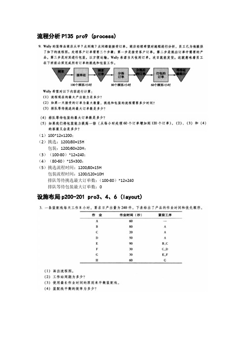
流程分析P135 pro9 (process)(1)100*12=1200;(2)挑选:1200/80=15H包装:1200/60=20H;(3)(100-80)*12=240;(4)(80-60)*15=300;(5)挑选流程时间:1200/80=15H包装流程时间:1200/120=10H排队等待挑选最大订单数:(100-80)*12=240排队等待包装最大订单数:0设施布局p200-201 pro3、4、6 (layout)a.b. C = production time per day/required output per day = (8 hour/day)(3600seconds/hour)/240 units per day = 120 seconds per unit c.Work station Task Task timeIdle timeIA D 60 50 10 IIB C 80 20 20 IIIE F 90 30 0 IVG H30 6030d. Efficiency =C N Ta = )120(4420 = .875 or 87.5%ABDCEFG30356530H35154025b. C = production time per day/required output per day = (450minutes/day)/360units per day = 1.25 minutes per unit or 75 seconds per unit c.Work stationTask Task timeIdle timeIAC E30 30 15 0 IIF 65 10 IIIBG 35 40 0 IVDH35 2515d. Efficiency =C N Ta = )75(4275 = .917 or 91.7%From/to Distances -rectilinear Flow Cost = distance Xflow X $2A toB 100’10 $2,000A to C 200’25 10,000A to D 250’55 27,500B toC 100’10 2,000B to D 150’ 5 1,500C toD 50’15 1,500Total $44,500过程能力和统计过程控制p314 1(1)(2),2(1),14 (SPC)Defective average = .04, inspection rate = 50 per hour, cost of inspector = $9 per hour, and repair cost is $10 each.a.No inspection .04 * (50) * $10 $20Inspection 9Therefore, it is cheaper to inspect in this case.b. Cost per unit for inspection = $9/50 = $.18a.{}333.1,889.min )003(.399.002.1,)003(.3002.101.1min 3,3min =⎭⎬⎫⎩⎨⎧--=⎭⎬⎫⎩⎨⎧--=σσLTL X X UTL C pk= .889X-double-bar —A2*R-bar2.03 – (.48*.35) = 1.852销售与运营计划p517 pro 3,4 (aggregate planning)Forecast BeginningInventory ProductionrequiredProduction hoursrequiredProduction hoursavailableOvertimehoursActualproductionEndinginventoryWorkershiredWorkerslaid offFebruary 80000 0 80000 20000 16000 80000 0 25*March 64000 0 64000 16000 16000 64000 0 25 April 100000 0 100000 25000 16000 5000 84000 -16000May 40000 -16000 56000 14000 16000 64000 8000Back order Overtime Hiring Lay off Inventory StraighttimeTotalFebruary $1,250 $200,000 $201,250 March $1,750 $160,000 $161,750 April $320,00$75,000 $160,000 $555,000May $80000 $160,000 $240,000 Total $1,158,000 *(20,000-16,000)/(8*20) = 25 workersForecast BeginningInventory ProductionrequiredProduction hoursrequiredProduction hoursavailableOvertimehoursActualproductionEndinginventoryWorkershiredWorkerslaid offSpring 20000 1000 19000 38000 28000 10000 19000 0Summer 10000 0 10000 20000 28000 10000 0 20 Fall 15000 0 15000 30000 20000 15000 0 25Winter 18000 0 18000 36000 30000 15000 -3000Back order Overtime Hiring Lay off Inventory StraighttimeTotalSpring $150,000 $280,000 $430,000 Summer $4,000 $200,000 $204,000 Fall $2,500 $300,000 $302,500 Winter $24,000 $300,000 $324,000 Total $1,260,50库存控制p548 pro8, 11, 27 (inventory)物料需求计划p576 pro 10,11(MRP)A B C(2)D(2)Lev el12DE(3)Least Total CostPeriod 1 2 3 4 5 6 7 8 9 10 Gross Requirements 30 50 10 20 70 80 20 60 200 50 On-hand 90 60 10 0 230 160 80 60 0 50 Net requirements 0 0 0 20 0 0 0 0 200 0 Planned order receipts 250 250 Planned order releases 250 250Least Unit CostPeriod 1 2 3 4 5 6 7 8 9 10 Gross Requirements 30 50 10 20 70 80 20 60 200 50 On-hand 90 60 10 0 430 360 280 260 200 0 Net requirements 0 0 0 20 0 0 0 0 0 50 Planned order receipts 450 50 Planned order releases 450 50CalculationsWeeks Quantityordered CarryingcostOrdercostTotal cost Unit cost4 20 $0.00 $10.00 $10.00 $0.5004 to5 90 0.70 10.00 10.70 0.1194 to 6 170 2.30 10.00 12.30 0.0724 to 7 190 2.90 10.00 12.90 0.0684 to 8 250 5.30 10.00 15.30 0.0614 to 9 450 15.30 10.00 25.30 0.0564 to 10 500 18.30 10.00 28.30 0.0579 200 0.00 10.00 10.009 to 10 250 2.50 10.00 12.50For Least Total Cost, order for periods 4 through 8, since carrying cost is the closest to ordering cost. For Least Unit Cost, order for periods 4 through 9, since this has the lowest unit cost.运营调度p600 pro3,9,12,17(scheduling)Car Customerpick-up time Remainingoverhaul timeNumber ofremainingoperationsSlack Slack per remainingoperationsA 10 4 1 6 6.0B 17 5 2 12 6.0C 15 1 3 14 4.7 Select car C first, then A and B tie for second.Job Process I Time Process II Time Order of Selection Position in SequenceA 4 5 2nd2ndB 16 14 5th3rdC 8 7 3rd5thD 12 11 4th4thE 3 9 1st1stJob CustomizingTime Painting Time Order of Selection Position in Sequence1 3.0 1.2 7th6th2 2.0 0.9 5th7th3 2.5 1.3 8th5th4 0.7 0.5 1st10th5 1.6 1.7 10th3rd6 2.1 0.8 4th8th7 3.2 1.4 9th4th8 0.6 1.8 2nd1st9 1.1 1.5 6th2nd10 1.8 0.7 3rd9thSOT: II-III-IV-I cost = (4 x $1,500) + (0 x $ 500) + (0 x $1,500) + (0 x $1,500) = $6,000FCFS: I-II-III-IV cost = (0 x $1,500) + (0 x $ 500) + (0 x $1,500) + (2 x $1,500) = $3,000EDD: I-II-III-IV cost = (0 x $1,500) + (0 x $ 500) + (0 x $1,500) + (2 x $1,500) = $3,000STR: I-III-IV-II cost = (0 x $1,500) + (2 x $ 500) + (0 x $1,500) + (1 x $1,500) = $2,500LPT: I-III-IV-II cost = (0 x $1,500) + (2 x $ 500) + (0 x $1,500) + (1 x $1,500) = $2,500STR and LPT are the lowest cost of the Priority rules, although two jobs are late in thisP55 pro7P101 pro6以上为教材页码。
《运营管理》课程习题及答案-修订版

《运营管理》课程习题及答案-修订版第1章运营管理概述习题⼀、单项选择题1、在组织的三⼤基本职能中,处于核⼼地位的是:()A、财务B、营销C、运营D、⼈⼒2、产品品种单⼀、产量⼤、⽣产重复程度⾼的⽣产类型称为()。
A、单件⽣产B、⼤量⽣产C、批量⽣产D、⼤批量⽣产3、⽣产设施按⼯艺流程布置,加⼯顺序固定不变,⼯艺过程的程序化、⾃动化程度较⾼的⽣产类型称为()A、连续型⽣产B、间断式⽣产C、订货式⽣产D、备货式⽣产4、有形产品的变换过程通常也称为()A.服务过程B.⽣产过程C.计划过程D.管理过程5、⽆形产品的变换过程有时称为()A.管理过程B.计划过程C.服务过程D.⽣产过程6、制造业企业与服务业企业最主要的⼀个区别是()A.产出的物理性质B.与顾客的接触程度C.产出质量的度量D.对顾客需求的响应时间7、企业经营活动中的最主要部分是()A.产品研发B.产品设计C.⽣产运营活动D.⽣产系统的选择8、下列哪项不是⽣产运作管理的⽬标()A、质量B、成本C、价格D、柔性9、按照⽣产要素密集程度和顾客接触程度划分,医院是:()A、⼤量资本密集服务B、⼤量劳动密集服务C、专业资本密集服务D、专业劳动密集服务10、当供不应求时,会出现下列情况:()A、供⽅之间竞争激化B、价格下跌C、出现回扣现象D、质量与服务⽔平下降⼆、多项选择题1、服务运营管理的特殊性体现在()A.设施规模较⼩B.质量易于度量C.对顾客需求的响应时间短D.产出不可储存E.可服务于有限区域范围内2、运营管理中的决策内容包括()A.运营战略决策B.运营系统运⾏决策C.运营组织决策D.运营系统设计决策E.营销决策3、产品结果⽆论有形还是⽆形,其共性表现在().A.市场畅销B.满⾜⼈们某种需要C.投⼊⼀定资源D.经过变换实现E..实现价值增值4、企业经营管理的职能有().A.财务管理B.技术管理C.运营管理D.营销管理E.⼈⼒资源管理5、运营管理的计划职能具体包括以下⽅⾯内容()A.⽬标B.原因C.⼈员D.地点E.时间F. ⽅式三、简答题1、根据⽣产活动的定义,⽣产活动有哪些含义?2、从管理的⾓度来看制造过程和服务过程,⼆者存在哪些重要异同?3、按照产品品种多少和⽣产的重复程度划分的⽣产类型有哪些?特点是什么?4、⽣产运营系统有哪些的主要特征?试对其进⾏简单描述。
《运营管理》课程习题及答案-修订版(1)

《运营管理》课程习题及答案-修订版(1)第1章运营管理概述习题⼀、单项选择题1、在组织的三⼤基本职能中,处于核⼼地位的是:()A、财务B、营销C、运营D、⼈⼒2、产品品种单⼀、产量⼤、⽣产重复程度⾼的⽣产类型称为()。
A、单件⽣产B、⼤量⽣产C、批量⽣产D、⼤批量⽣产3、⽣产设施按⼯艺流程布置,加⼯顺序固定不变,⼯艺过程的程序化、⾃动化程度较⾼的⽣产类型称为()A、连续型⽣产B、间断式⽣产C、订货式⽣产D、备货式⽣产4、有形产品的变换过程通常也称为()A.服务过程B.⽣产过程C.计划过程D.管理过程5、⽆形产品的变换过程有时称为()A.管理过程B.计划过程C.服务过程D.⽣产过程6、制造业企业与服务业企业最主要的⼀个区别是()A.产出的物理性质B.与顾客的接触程度C.产出质量的度量D.对顾客需求的响应时间7、企业经营活动中的最主要部分是()A.产品研发B.产品设计C.⽣产运营活动D.⽣产系统的选择8、下列哪项不是⽣产运作管理的⽬标()A、质量B、成本C、价格D、柔性9、按照⽣产要素密集程度和顾客接触程度划分,医院是:()A、⼤量资本密集服务B、⼤量劳动密集服务C、专业资本密集服务D、专业劳动密集服务10、当供不应求时,会出现下列情况:()A、供⽅之间竞争激化B、价格下跌C、出现回扣现象D、质量与服务⽔平下降⼆、多项选择题1、服务运营管理的特殊性体现在()A.设施规模较⼩B.质量易于度量C.对顾客需求的响应时间短D.产出不可储存E.可服务于有限区域范围内2、运营管理中的决策内容包括()A.运营战略决策B.运营系统运⾏决策C.运营组织决策3、产品结果⽆论有形还是⽆形,其共性表现在().A.市场畅销B.满⾜⼈们某种需要C.投⼊⼀定资源D.经过变换实现E..实现价值增值4、企业经营管理的职能有().A.财务管理B.技术管理C.运营管理D.营销管理E.⼈⼒资源管理5、运营管理的计划职能具体包括以下⽅⾯内容()A.⽬标B.原因C.⼈员D.地点E.时间F. ⽅式三、简答题1、根据⽣产活动的定义,⽣产活动有哪些含义?2、从管理的⾓度来看制造过程和服务过程,⼆者存在哪些重要异同?3、按照产品品种多少和⽣产的重复程度划分的⽣产类型有哪些?特点是什么?4、⽣产运营系统有哪些的主要特征?试对其进⾏简单描述。
《运营管理》课后习题答案
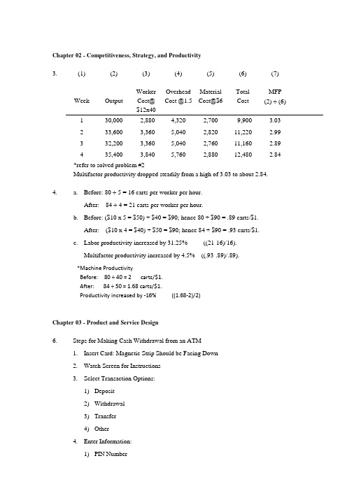
Chapter 02 - Competitiveness, Strategy, and Productivity3. (1) (2) (3) (4) (5) (6) (7)Week Output WorkerCost@$12x40OverheadCost @1.5MaterialCost@$6TotalCostMFP(2) ÷ (6)1 30,000 2,880 4,320 2,700 9,900 3.032 33,600 3,360 5,040 2,820 11,220 2.993 32,200 3,360 5,040 2,760 11,160 2.894 35,400 3,840 5,760 2,880 12,480 2.84*refer to solved problem #2Multifactor productivity dropped steadily from a high of 3.03 to about 2.84.4. a. Before: 80 ÷ 5 = 16 carts per worker per hour.After: 84 ÷ 4 = 21 carts per worker per hour.b. Before: ($10 x 5 = $50) + $40 = $90; hence 80 ÷ $90 = .89 carts/$1.After: ($10 x 4 = $40) + $50 = $90; hence 84 ÷ $90 = .93 carts/$1.c. Labor productivity increased by 31.25% ((21-16)/16).Multifactor productivity increased by 4.5% ((.93-.89)/.89).*Machine ProductivityBefore: 80 ÷ 40 = 2 carts/$1.After: 84 ÷ 50 = 1.68 carts/$1.Productivity increased by -16% ((1.68-2)/2)Chapter 03 - Product and Service Design6. Steps for Making Cash Withdrawal from an ATM1. Insert Card: Magnetic Strip Should be Facing Down2. Watch Screen for Instructions3. Select Transaction Options:1) Deposit2) Withdrawal3) Transfer4) Other4. Enter Information:1) PIN Number2) Select a Transaction and Account3) Enter Amount of Transaction5. Deposit/Withdrawal: 1) Deposit —place in an envelope (which you’ll find near or in the ATM) andinsert it into the deposit slot2) Withdrawal —lift the “Withdrawal Door,” being careful to remove all cash6. Remove card and receipt (which serves as the transaction record)8.Chapter 04 - Strategic Capacity Planning for Products and Services2. %80capacityEf f ective outputActual Ef f iciency ==Actual output = .8 (Effective capacity) Effective capacity = .5 (Design capacity) Actual output = (.5)(.8)(Effective capacity) Actual output = (.4)(Design capacity) Actual output = 8 jobs Utilization = .4capacityDesign outputActual =n Utilizatiojobs 204.8capacity Ef f ective output Actual Capacity Design ===10. a. Given: 10 hrs. or 600 min. of operating time per day.250 days x 600 min. = 150,000 min. per year operating time.Solutions_Problems_OM_11e_Stevenson3 / 22Total processing time by machineProductABC 1 48,000 64,000 32,000 2 48,000 48,000 36,000 3 30,000 36,000 24,000 460,000 60,000 30,000 Total 186,000208,000122,000machine181.000,150000,122machine 238.1000,150000,208machine224.1000,150000,186≈==≈==≈==C B A N N NYou would have to buy two “A” machines at a total cost of $80,000, or two “B” machines at a total cost of $60,000, or one “C” machine at $80,000.b.Total cost for each type of machine:A (2): 186,000 min ÷ 60 = 3,100 hrs. x $10 = $31,000 + $80,000 = $111,000B (2) : 208,000 ÷ 60 = 3,466.67 hrs. x $11 = $38,133 + $60,000 = $98,133 C(1): 122,000 ÷ 60 = 2,033.33 hrs. x $12 = $24,400 + $80,000 = $104,400Buy 2 Bs —these have the lowest total cost.Chapter 05 - Process Selection and Facility Layout3.Desired output = 4Operating time = 56 minutesunit per minutes 14hourper units 4hourper minutes 65output Desired time Operating CT ===Task # of Following tasksPositional WeightA 4 23B 3 20C 2 18D 3 25E 2 18F 4 29G 3 24H 1 14 I5a. First rule: most followers. Second rule: largest positional weight.Assembly Line Balancing Table (CT = 14)Solutions_Problems_OM_11e_Stevenson5 / 22b. First rule: Largest positional weight.Assembly Line Balancing Table (CT = 14)c. %36.805645stations of no. x CT time Total Ef f iciency ===4. a. l.2. Minimum Ct = 1.3 minutesTask Following tasksa 4b 3c 3d 2e 3f 2g 1h3. percent 54.11)3.1(46.CT x N time)(idle percent Idle ==∑=4. 420 min./day 323.1 ( 323)/1.3 min./OT Output rounds to copiers day CT cycle=== b. 1. inutes m 3.224.6N time Total CT ,6.4 time Total ==== 2. Assign a, b, c, d, and e to station 1: 2.3 minutes [no idle time]Assign f, g, and h to station 2: 2.3 minutes3. 420182.6 copiers /2.3OT Output day CT ===4.420 min./dayMaximum Ct is 4.6. Output 91.30 copiers /4.6 min./day cycle==7.Solutions_Problems_OM_11e_Stevenson7 / 22Chapter 06 - Work Design and Measurement3.Element PR OT NT AF job ST1 .90.46.414 1.15 .4762 .85 1.505 1.280 1.15 1.4723 1.10.83.913 1.15 1.05041.00 1.16 1.160 1.15 1.334Total4.3328. A = 24 + 10 + 14 = 48 minutes per 4 hours.min 125.720.11x70.5ST .min 70.5)95(.6NT 20.24048A =-=====9. a. Element PR OT NT A ST1 1.10 1.19 1.309 1.15 1.5052 1.15 .83 .955 1.15 1.09831.05.56.588 1.15 .676b.01.A 00.2z 034.s 83.x ==== 222(.034)67.12~68.01(.83)zs n observations ax ⎛⎫⎛⎫===⎪ ⎪⎝⎭⎝⎭ c. e = .01 minutes 47 to round ,24.4601.)034(.2e zs n 22=⎪⎭⎫⎝⎛=⎪⎭⎫ ⎝⎛=Chapter 07- Location Planning and Analysis1. Factor Local bank Steel mill Food warehouse Public school1. Convenience forcustomers H L M–H M–H2. Attractiveness ofbuilding H L M M–H3. Nearness to rawmaterials L H L M4. Large amounts ofpower L H L L5. Pollution controls L H L L6. Labor cost andavailability L M L L7. Transportationcosts L M–H M–H M8. Constructioncosts M H M M–HLocation (a) Location (b)4. Factor A B C Weight A B C1. Business Services 9 5 5 2/9 18/9 10/9 10/92. Community Services 7 6 7 1/9 7/9 6/9 7/93. Real Estate Cost 3 8 7 1/9 3/9 8/9 7/94. Construction Costs 5 6 5 2/9 10/9 12/9 10/95. Cost of Living 4 7 8 1/9 4/9 7/9 8/96. Taxes 5 5 5 1/9 5/9 5/9 4/97. Transportation 6 7 8 1/9 6/9 7/9 8/9Total 39 44 45 1.0 53/9 55/9 54/9 Each factor has a weight of 1/7.a. Composite Scores 39 44 45 7 7 7B orC is the best and A is least desirable.b. Business Services and Construction Costs both have a weight of 2/9; the other factors eachhave a weight of 1/9.5 x + 2 x + 2 x = 1 x = 1/9c. Composite ScoresA B C 53/9 55/9 54/9B is the best followed byC and then A.Solutions_Problems_OM_11e_Stevenson9 / 225. Location x yA3 7 B 8 2 C4 6 D4 1E 6 4 Totals 25 20-x = ∑x i = 25 = 5.0-y =∑y i = 20= 4.0n5n5Hence, the center of gravity is at (5,4) and therefore the optimal location.Chapter 08 - Management of Quality1.ChecksheetWork Type FrequencyLube and Oil 12 Brakes 7 Tires 6 Battery 4 Transmission1Total30ParetoLube & Oil BrakesTiresBatteryTrans.2 .The run charts seems to show a pattern of errors possibly linked to break times or the end of the shift. Perhaps workers are becoming fatigued. If so, perhaps two 10 minute breaks in the morning and again in the afternoon instead of one 20 minute break could reduce some errors. Also, errors are occurring during the last few minutes before noon and the end of the shift, and those periods should also b e given management’s attention.4break lunch break3 2 1 0∙ ∙ ∙∙ ∙ ∙ ∙∙∙ ∙ ∙ ∙∙∙∙∙∙∙ ∙∙∙ ∙∙ ∙ ∙∙ ∙ ∙∙∙Solutions_Problems_OM_11e_Stevenson11 / 22Chapter 9 - Quality Control4. Sample Mean Range179.48 2.6 Mean Chart: =X ± A 2-R = 79.96 ± 0.58(1.87) 2 80.14 2.3 = 79.96 ± 1.083 80.14 1.2UCL = 81.04, LCL = 78.884 79.60 1.7 Range Chart: UCL = D 4-R = 2.11(1.87) = 3.95 5 80.02 2.0LCL = D 3-R = 0(1.87) = 0680.381.4[Both charts suggest the process is in control: Neither has any points outside the limits.]6. n = 200 Control Limits = np p p )1(2-±Thus, UCL is .0234 and LCL becomes 0.Since n = 200, the fraction represented by each data point is half the amount shown. E.g., 1 defective = .005, 2 defectives = .01, etc.Sample 10 is too large.7. 857.714110c == Control limits: 409.8857.7c 3c ±=± UCL is 16.266, LCL becomes 0.All values are within the limits.14. Let USL = Upper Specification Limit, LSL = Lower Specification Limit,= Process mean, σ = Process standard deviationFor process H:}{capablenot ,0.193.93.04.1 ,938.min 04.1)32)(.3(1516393.)32)(.3(1.14153<===-=σ-=-=σ-pk C X USL LSL X 0096.)200(1325==p 0138.0096.200)9904(.0096.20096.±=±=For process K:.1}17.1,0.1min{17.1)1)(3(335.3630.1)1)(3(30333===-=σ-=-=σ- C X USL LSL X pk Assuming the minimum acceptable pk C is 1.33, since 1.0 < 1.33, the process is not capable.For process T:33.1}33.1,67.1min{33.1)4.0)(3(5.181.20367.1)4.0)(3(5.165.183===-=σ-=-=σ- C X USL LSL X pk Since 1.33 = 1.33, the process is capable.Chapter 10 - Aggregate Planning and Master Scheduling7. a. No backlogs are allowedPeriodForecast Output Regular Overtime Subcontract Output - Forecast Inventory Beginning Ending Average Backlog Costs: Regular Overtime Subcontract Inventory TotalSolutions_Problems_OM_11e_Stevenson13 / 22b.Level strategyPeriodForecast Output Regular Overtime Subcontract Output - Forecast Inventory Beginning Ending Average Backlog Costs: Regular Overtime Subcontract Inventory Backlog Total8.Period Forecast Output Regular Overtime Subcontract Output- Forecast Inventory Beginning Ending Average Backlog Costs: Regular Overtime Subcontract Inventory Backlog TotalChapter 11 - MRP and ERP1. a. F: 2G: 1H: 1J: 2 x 2 = 4 L: 1 x 2 = 2 A: 1 x 4 = 4 D: 2 x 4 = 8 J: 1 x 2 = 2 D: 1 x 2 = 2Totals: F = 2; G = 1; H = 1; J = 6; D = 10; L = 2; A = 44. Master ScheduleSolutions_Problems_OM_11e_Stevenson10. Week 1 2 3 4Material 40 80 60 70Week 1 2 3 4Labor hr. 160 320 240 280Mach. hr. 120 240 180 210a. Capacity utilizationWeek 1 2 3 4Labor 53.3% 106.7% 80% 93.3%Machine 60% 120% 90% 105%b. C apacity utilization exceeds 100% for both labor and machine in week 2, and formachine alone in week 4.Production could be shifted to earlier or later weeks in which capacity isunderutilized. Shifting to an earlier week would result in added carrying costs;shifting to later weeks would mean backorder costs.Another option would be to work overtime. Labor cost would increase due toovertime premium, a probable decrease in productivity, and possible increase inaccidents.15 / 22Chapter 12 - Inventory Management2.The following table contains figures on the monthly volume and unit costs for a random sample of 16 items for a list of 2,000 inventory items.a. See table.b. To allocate control efforts.c. It might be important for some reason other than dollar usage, such as cost of astockout, usage highly correlated to an A item, etc.3. D = 1,215 bags/yr. S = $10 H = $75a. bags HDS Q 187510)215,1(22===b. Q/2 = 18/2 = 9 bagsc.orders ordersbags bags Q D 5.67/ 18 215,1== d . S QD H 2/Q TC +=Solutions_Problems_OM_11e_Stevenson17 / 22350,1$675675)10(18215,1)75(218=+=+=e. Assuming that holding cost per bag increases by $9/bag/yearQ ==84)10)(215,1(217 bags71.428,1$71.714714)10(17215,1)84(217=+=+=TCIncrease by [$1,428.71 – $1,350] = $78.714.D = 40/day x 260 days/yr. = 10,400 packagesS = $60 H = $30a. oxes b 20496.2033060)400,10(2H DS 2Q 0====b. S QD H 2Q TC +=82.118,6$82.058,3060,3)60(204400,10)30(2204=+=+=c. Yesd. )60(200400,10)30(2200TC 200+=TC 200 = 3,000 + 3,120 = $6,1206,120 – 6,118.82 (only $1.18 higher than with EOQ, so 200 is acceptable.)7.H = $2/month S = $55D 1 = 100/month (months 1–6)D 2 = 150/month (months 7–12)a. 16.74255)100(2Q :D H DS2Q 010===83.90255)150(2Q :D 02==b. The EOQ model requires this.c. Discount of $10/order is equivalent to S – 10 = $45 (revised ordering cost)1–6 TC74 = $148.32180$)45(150100)2(2150TC 145$)45(100100)2(2100TC *140$)45(50100)2(250TC 15010050=+==+==+=7–12 TC 91 =$181.66195$)45(150150)2(2150TC *5.167$)45(100150)2(2100TC 185$)45(50150)2(250TC 15010050=+==+==+=10. p = 50/ton/day u = 20 tons/day200 days/yr.S = $100 H = $5/ton per yr.a. bags] [10,328 tons 40.5162050505100)000,4(2u p p H DS 2Q 0=-=-=b. ]bags 8.196,6 .approx [ tons 84.309)30(504.516)u p (P Q I max ==-=Average is92.154248.309:2I max =tons [approx. 3,098 bags] c. Run length =days 33.10504.516P Q == d. Runs per year = 8] approx.[ 7.754.516000,4QD == e. Q ' = 258.2TC =S QD H 2I max + TC orig. = $1,549.00 TC rev. = $ 774.50Savings would be $774.50D= 20 tons/day x 200 days/yr. = 4,000 tons/yr.Solutions_Problems_OM_11e_Stevenson19 / 2215. RangeP H Q D = 4,900 seats/yr. 0–999 $5.00 $2.00 495 H = .4P 1,000–3,999 4.95 1.98 497 NF S = $50 4,000–5,999 4.90 1.96 500 NF 6,000+ 4.85 1.94503 NFCompare TC 495 with TC for all lower price breaks:TC 495 = 495 ($2) + 4,900($50) + $5.00(4,900) = $25,4902 495 TC 1,000 = 1,000 ($1.98) + 4,900($50) + $4.95(4,900) = $25,4902 1,000 TC 4,000 = 4,000 ($1.96) + 4,900($50) + $4.90(4,900) = $27,9912 4,000 TC 6,000 = 6,000 ($1.94) + 4,900($50) + $4.85(4,900) = $29,6262 6,000Hence, one would be indifferent between 495 or 1,000 units22. d = 30 gal./day ROP = 170 gal. LT = 4 days,ss = Z σd LT = 50 galRisk = 9% Z = 1.34 Solving, σd LT = 37.31 3% Z = 1.88, ss=1.88 x 37.31 = 70.14 gal.Chapter 13 - JIT and Lean Operations1. N = ?N = DT(1 + X)D = 80 pieces per hourC T = 75 min. = 1.25 hr. = 80(1.25) (1.35)= 3C = 45 45X = .35QuantityTC4. The smallest daily quantity evenly divisible into all four quantities is 3. Therefore, usethree cycles.Product Daily quantity Units per cycleA 21 21/3 = 7B 12 12/3 = 4C 3 3/3 = 1D 15 15/3 = 55.a. Cycle 1 2 3 4A 6 6 5 5B 3 3 3 3C 1 1 1 1D 4 4 5 5E 2 2 2 2 b. Cycle 1 2A 11 11B 6 6C 2 2D 8 8E 4 4c. 4 cycles = lower inventory, more flexibility2 cycles = fewer changeovers7. Net available time = 480 – 75 = 405. Takt time = 405/300 units per day = 1.35 minutes. Chapter 15 - Scheduling6. a. FCFS: A–B–C–DSPT: D–C–B–AEDD: C–B–D–ACR: A–C–D–BFCFS: Job time Flow time Due date DaysJob (days) (days) (days) tardyA 14 14 20 0B 10 24 16 8C 7 31 15 16D 6 37 17 2037 106 44Solutions_Problems_OM_11e_Stevenson21 / 22SPT: Job time Flow time Due date Days Job (days) (days) (days) tardy D 6 6 17 0 C 7 13 15 0 B 10 23 16 7 A 14 37 20 17377924EDD:Job D has the lowest critical ratio therefore it is scheduled next and completed on day 27.b.ardi Flow time Average flow time Number of jobsDays tardy Average job t ness Number of jobs Flow timeAverage number of jobs at the center Makespan==∑=FCFS SPT EDD CR26.50 19.75 21.00 24.75 11.0 6.00 6.00 9.252.86 2.142.272.67c. SPT is superior.9.Thus, the sequence is b-a-g-e-f-d-c.。
《运营管理》课后习题答案

Chapter 02 — Competitiveness,Strategy, and Productivity3. (1)(2) (3) (4) (5) (6) (7)Week Output WorkerCost@$12x40OverheadCost @1.5MaterialCost@$6TotalCostMFP(2) ÷ (6)1 30,000 2,880 4,320 2,700 9,900 3.032 33,600 3,360 5,040 2,820 11,220 2。
993 32,200 3,360 5,040 2,760 11,160 2.894 35,400 3,840 5,760 2,880 12,480 2.84*refer to solved problem #2Multifactor productivity dropped steadily from a high of 3.03 to about 2。
84。
4。
a。
Before: 80 ÷ 5 = 16 carts per worker per hour.After: 84 ÷ 4 = 21 carts per worker per hour.b。
Before:($10 x 5 = $50)+ $40 = $90; hence 80 ÷$90 = .89 carts/$1.After:($10 x 4 = $40) + $50 = $90; hence 84 ÷ $90 = .93 carts/$1.c. Labor productivity increased by 31。
25%((21—16)/16).Multifactor productivity increased by 4.5% ((。
93-.89)/。
89).*Machine ProductivityBefore: 80 ÷ 40 = 2 carts/$1.After:84 ÷ 50 = 1.68 carts/$1.Productivity increased by —16% ((1。
《运营管理》教材作业参考答案
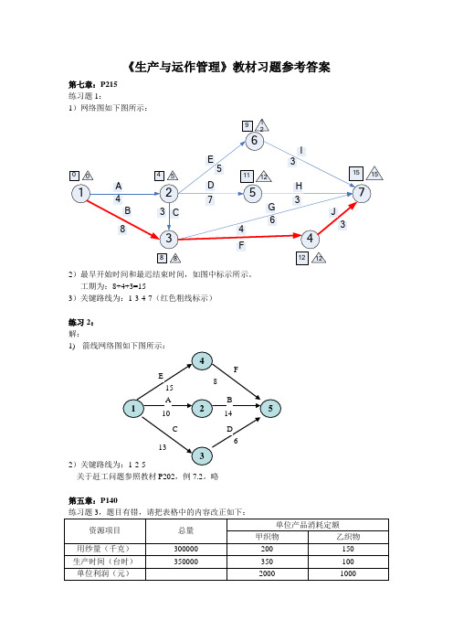
《生产与运作管理》教材习题参考答案第七章:P215 练习题1:1)网络图如下图所示:2)最早开始时间和最迟结束时间,如图中标示所示。
工期为:8+4+3=153)关键路线为:1-3-4-7(红色粗线标示)练习2: 解:1)2 关于赶工问题参照教材P202,例7.2。
略第五章:P140答案参见教材:P118,例5.6,略第四章:P95 练习题1:12)车间布置:根据关系分数排序,题目条件或约束,确定好车间7、2、4、1(注意车间1不能位于厂区中间位置,故列于最左下);车间3与车间2的关系为A ,故安排于其左或右;车间8与车间4关系为A ,可安排于其上或其右;车间3、5、8的安排根据其相邻的所有车间的关系密切程度之和可以计算(略),可知车间5位于车间4上,车间8位于车间4右,车间3位于车间1上。
车间6与车间8的关系为A ,故车间6位于车间8上。
最终结果如图示:第三章:P61练习题1:解:Y=0.5X40+0.35X30+0.20X10=32.5 城市2综合得分高,因此是最佳选择。
练习题3. 解:设采用营口冷库,则如下表所示:其运输总费用=210*10+60*12+70*17+10*20+150*11+160*7=6980 由此可知,采用营口冷库更佳。
练习题5:解:首先,建立地图坐标系 9 8 7 65 4 3 2 11 23 4 5 6 7 8 9 10 11 设处理中心(X ,Y ),则利用重心法公式计算如下:∑∑=ii i Q Q x X /)403025926/()408302254942610(++++⨯+⨯+⨯+⨯+⨯==6∑∑=i i i Q Q y Y /)403025926/()40730625791265(++++⨯+⨯+⨯+⨯+⨯==6处理中心坐标为(6,6),位置如图中红色点标示。
第九章:P302 练习题1:解:这是一个存在折扣的库存模型问题。
1) 无论订购多少,订购单价为10元时,库存维持费为:H=10*10%=1 ,订货费用S=225 年需求量为:D=3600,则:EOQ (10)=12731225360022=⨯⨯=H DS单位2) 当订购量为大于等于500时,库存维持费为:H=9*10%=0.9,订货费用S=225,年需求量为:D=3600,则: EOQ (9)=13429.0225360022=⨯⨯=H DS单位3) 当订购量为大于等于1000时,库存维持费为:H=8*10%=0.8,订货费用S=225,年需求量为:D=3600,则: EOQ (8)=14238.0225360022=⨯⨯=H DS单位以上三种经济订货量单位都大于1000的订量单位,显然都是可行的订货量。
《运营管理》课程习题和答案解析_修订版
第1章运营管理概述习题一、单项选择题1、在组织的三大基本职能中,处于核心地位的是:()A、财务B、营销C、运营D、人力2、产品品种单一、产量大、生产重复程度高的生产类型称为()。
A、单件生产B、大量生产C、批量生产D、大批量生产3、生产设施按工艺流程布置,加工顺序固定不变,工艺过程的程序化、自动化程度较高的生产类型称为()A、连续型生产B、间断式生产C、订货式生产D、备货式生产4、有形产品的变换过程通常也称为()A.服务过程B.生产过程C.计划过程D.管理过程5、无形产品的变换过程有时称为()A.管理过程B.计划过程C.服务过程D.生产过程6、制造业企业与服务业企业最主要的一个区别是()A.产出的物理性质B.与顾客的接触程度C.产出质量的度量D.对顾客需求的响应时间7、企业经营活动中的最主要部分是()A.产品研发B.产品设计C.生产运营活动D.生产系统的选择8、下列哪项不是生产运作管理的目标()A、质量B、成本C、价格D、柔性9、按照生产要素密集程度和顾客接触程度划分,医院是:()A、大量资本密集服务B、大量劳动密集服务C、专业资本密集服务D、专业劳动密集服务10、当供不应求时,会出现下列情况:()A、供方之间竞争激化B、价格下跌C、出现回扣现象D、质量与服务水平下降二、多项选择题1、服务运营管理的特殊性体现在()A.设施规模较小B.质量易于度量C.对顾客需求的响应时间短D.产出不可储存E.可服务于有限区域范围内2、运营管理中的决策内容包括()A.运营战略决策B.运营系统运行决策C.运营组织决策D.运营系统设计决策E.营销决策3、产品结果无论有形还是无形,其共性表现在().A.市场畅销B.满足人们某种需要C.投入一定资源D.经过变换实现E..实现价值增值4、企业经营管理的职能有().A.财务管理B.技术管理C.运营管理D.营销管理E.人力资源管理5、运营管理的计划职能具体包括以下方面内容()A.目标B.原因C.人员D.地点E.时间F. 方式三、简答题1、根据生产活动的定义,生产活动有哪些含义?2、从管理的角度来看制造过程和服务过程,二者存在哪些重要异同?3、按照产品品种多少和生产的重复程度划分的生产类型有哪些?特点是什么?4、生产运营系统有哪些的主要特征?试对其进行简单描述。
- 1、下载文档前请自行甄别文档内容的完整性,平台不提供额外的编辑、内容补充、找答案等附加服务。
- 2、"仅部分预览"的文档,不可在线预览部分如存在完整性等问题,可反馈申请退款(可完整预览的文档不适用该条件!)。
- 3、如文档侵犯您的权益,请联系客服反馈,我们会尽快为您处理(人工客服工作时间:9:00-18:30)。
B
3
20
C
2
18
D
3
25
E
2
18
F
4
29
G
3
24
H
1
14
/3 20
Solutions_Problems_OM_11e_Stevenson
I
0
5
a. First rule: most followers. Second rule: largest positional weight. Assembly Line Balancing Table (CT = 14)
1.00 1.16 1.160 1.15 1.334
Total
4.332
8.
A = 24 + 10 + 14 = 48 minutes per 4 hours
A = 48 = .20 240
NT = 6(.95) = 5.70 min .
ST = 5.70x 1 = 7.125 min . 1 − .20
2) Withdrawal—lift the “Withdrawal Door,” being careful to remove all cash 6. Remove card and receipt (which serves as the transaction record)
8.
Technical Requirements Customer Requirements
Buy 2 Bs—these have the lowest total cost. Chapter 05 - Process Selection and Facility Layout
3.
3
2
4
a
b
c
Desired output = 4
Operati7ng time = 56 minutes
4
9
5
5. Deposit/Withdrawal:
/1 20
Solutions_Problems_OM_11e_Stevenson
1) Deposit—place in an envelope (which you’ll find near or in the ATM) and insert it into the deposit slot
Total Cost
MFP (2) (6)
1
30,000
2,880 4,320
2,700
9,900
3.03
2
33,600
3,360 5,040
2,820
11,220
2.99
3
32,200
3,360 5,040
2,760
11,160
2.89
4
35,400
3,840 5,760
2,880
12,480
2.84
4. c
/4 20
a
b
d
h
a. l.
Solutions_Problems_OM_11e_Stevenson
2. Minimum Ct = 1.3 minutes
Task Following tasks
a
4
b
3
c
3
d
2
e
3
f
2
g
1
h
0
Work Station I
Eligible a
b,c,e, (tie)
Utilization = Actual output Design capacity
Design Capacity = Actualoutput = 8 = 20 jobs Effective capacity .4
10. a. Given: 10 hrs. or 600 min. of operating time per day. 250 days x 600 min. = 150,000 min. per year operating time.
Total processing time by machine
Product 1
A 48,000
B 64,000
C 32,000
2
48,000 48,000 36,000
3
30,000 36,000 24,000
/2 20
Solutions_Problems_OM_11e_Stevenson
4 Total
Chapter 03 - Product and Service Design 6. Steps for Making Cash Withdrawal from an ATM
1. Insert Card: Magnetic Strip Should be Facing Down
2. Watch Screen for Instructions
c. Labor productivity increased by 31.25% ((21-16)/16).
Multifactor productivity increased by 4.5% ((.93-.89)/.89).
*Machine Productivity Before: 80 ÷ 40 = 2 carts/$1. After: 84 ÷ 50 = 1.68 carts/$1. Productivity increased by -16% ((1.68-2)/2)
3. Select Transaction Options:
1) Deposit
2) Withdrawal
3) Transfer
4) Other
4. Enter Information:
1) PIN Number
2) Select a Transaction and Account
3) Enter Amount of Transaction
7.
1
5
4
3
8
7
6
2
Chapter 06 - Work Design and Measurement
3.
Element PR OT
NT
AFjob
ST
1
.90 .46 .414 1.15 .476
2
.85 1.505 1.280 1.15 1.472
3
1.10 .83 .913 1.15 1.050
4
Solutions_Problems_OM_11e_Stevenson
Chapter 02 - Competitiveness, Strategy, and Productivity
3.
(1)
(2)
(3)
(4)
(5)
(6)
(7)
Week
Output
Worker Cost@ $12x40
Overhead Material Cost @1.5 Cost@$6
9.
a. Element PR OT NT
A
ST
1
1.10 1.19 1.309 1.15 1.505
2
1.15 .83 .955 1.15 1.098
3
1.05 .56 .588 1.15 .676
b.
x = .83 s = .034 z = 2.00 A = .01
n
=
zs ax
2
=
After: 84 4 = 21 carts per worker per hour.
b. Before: ($10 x 5 = $50) + $40 = $90; hence 80 ÷$90 = .89 carts/$1.
After: ($10 x 4 = $40) + $50 = $90; hence 84 ÷$90 = .93 carts/$1.
*refer to solved problem #2 Multifactor productivity dropped steadily from a high of 3.03 to about 2.84.
4. a. Before: 80 5 = 16 carts per worker per hour.
Taste
Ingredients √
Appearance
√
Texture/consistency
√
Handling √
Preparation
√ √ √
Chapter 04 - Strategic Capacity Planning for Products and Services
2.
Efficiency = Actualoutput = 80%
60,000 186,000
60,000 208,000
30,000 122,000
NA
=
186,000 150,000
= 1.24
2
machine
208,000 NB = 150,000 = 1.38 2 machine
NC
=
122,000 150,000
= .81 1 machine
You would have to buy two “A” machines at a total cost of $80,000, or two “B” machines at a total cost of $60,000, or one “C” machine at $80,000. b. Total cost for each type of machine:
A (2): 186,000 min 60 = 3,100 hrs. x $10 = $31,000 + $80,000 = $111,000