曼昆微观经济学第13章习题答案
曼昆 微观经济学 原理 第五版 课后习题答案
曼昆微观经济学原理第五版课后习题答案曼昆-微观经济学-原理-第五版-课后习题答案问题与应用1.描绘以下每种情况所遭遇的权衡权衡:a.一个家庭同意与否卖一辆新车。
答:如果买新车就要减少家庭其他方面的开支,如:外出旅行,购置新家具;如果不买新车就享受不到驾驶新车外出的方便和舒适。
b.国会议员决定对国家公园支出多少。
请问:对国家公园的开支数额小,国家公园的条件可以获得提升,环境可以获得更好的维护。
但同时,政府可以用作交通、邮电等其他公共事业的开支就可以增加。
c.一个公司总裁同意与否崭新上开一家工厂。
答:开一家新厂可以扩大企业规模,生产更多的产品。
但可能用于企业研发的资金就少了。
这样,企业开发新产品、利用新技术的进度可能会减慢。
d.一个教授决定用多少时间备课。
请问:教授若将大部分时间用作自己研究,可能会出来更多成果,但复习时间增加影响学生讲课质量。
e.一个刚大学毕业的学生决定是否去读研究生。
请问:毕业后出席工作,可以即刻以获取工资收入;但稳步念研究生,能够拒绝接受更多科学知识和未来更高收益。
2.你正想决定是否去度假。
度假的大部分成本((机票、旅馆、放弃的工资))都用美元来衡量,但度假的收益是心理的。
你将如何比较收益与成本呢??请问:这种心理上的收益可以用与否达至既定目标去来衡量。
对于这个行动前就可以做出的既定目标,我们一定存有一个为实现目标而愿分担的成本范围。
在这个可以忍受的成本范围内,渡假如果满足用户了既定目标,例如:收紧身心、恢复正常体力等等,那么,就可以说道这次渡假的收益至少不大于它的成本。
3.你正计划用星期六回去专门从事业余工作,但一个朋友恳请你回去滑雪。
回去滑雪的真实成本就是什么?现在假设你已计划这天在图书馆自学,这种情况下去滑雪的成本就是什么?恳请表述之。
请问:回去滑雪的真实成本就是周六打零工所要赚的工资,我本可以利用这段时间回去工作。
如果我本计划这天在图书馆自学,那么回去滑雪的成本就是在这段时间里我可以赢得的科学知识。
曼昆微观经济学课后练习英文答案完整版

曼昆微观经济学课后练习英文答案集团标准化办公室:[VV986T-J682P28-JP266L8-68PNN]the link between buyers’ willingness to pay for a good and the demandcurve.how to define and measure consumer surplus.the link between sellers’ costs of producing a good and the supply curve.how to define and measure producer surplus.that the equilibrium of supply and demand maximizes total surplus in amarket.CONTEXT AND PURPOSE:Chapter 7 is the first chapter in a three-chapter sequence on welfare economics and market efficiency. Chapter 7 employs the supply and demand model to develop consumer surplus and producer surplus as a measure of welfare and market efficiency. These concepts are then utilized in Chapters 8 and 9 to determine the winners and losers from taxation and restrictions on international trade.The purpose of Chapter 7 is to develop welfare economics—the study of how the allocation of resources affects economic well-being. Chapters 4 through 6 employed supply and demand in a positive framework, which focused on the question, “What is the equilibrium price and quantity in a market” This chapter now addresses the normative question, “Is the equilibrium price and quantity in a market the best possible solution to the resource allocation problem, or is it simply the price and quantity that balance supply and demand” Students will discover that under most circumstances the equilibrium price and quantity is also the one that maximizes welfare.KEY POINTS:Consumer surplus equals buyers’ willingness to pay for a good minus the amount they actually pay for it, and it measures the benefit buyers get from participating in a market. Consumer surplus can be computed by finding the area below the demand curve and above the price.Producer surplus equals the amount sellers receive for their goods minus their costs of production, and it measures the benefit sellers get from participating in a market. Producer surplus can be computed by finding the area below the price and above the supply curve.An allocation of resources that maximizes the sum of consumer and producer surplus is said to be efficient. Policymakers are often concerned with the efficiency, as well as the equality, of economic outcomes.The equilibrium of supply and demand maximizes the sum of consumer andproducer surplus. That is, the invisible hand of the marketplace leadsbuyers and sellers to allocate resources efficiently.Markets do not allocate resources efficiently in the presence of market failures such as market power or externalities.CHAPTER OUTLINE:I. Definition of welfare economics: the study of how the allocation of resources affects economic well-being.A. Willingness to Pay1. Definition of willingness to pay: the maximum amount that a buyer will pay for a good.2. Example: You are auctioning a mint-condition recording of Elvis Presley’s first album. Four buyers show up. Their willingness to pay is as follows:If the bidding goes to slightly higher than $80, all buyersdrop out except for John. Because John is willing to paymore than he has to for the album, he derives some benefitfrom participating in the market.3. Definition of consumer surplus: the amount a buyer is willing to payfor a good minus the amount the buyer actually pays for it.4. Note that if you had more than one copy of the album, the price in the auction would end up being lower (a little over $70 in the case of two albums) and both John and Paul would gain consumer surplus.B. Using the Demand Curve to Measure Consumer Surplus1. We can use the information on willingness to pay to derive a demandmarginal buyer . Because the demand curve shows the buyers’ willingness to pay, we can use the demand curve to measure c onsumer surplus.C. How a Lower Price Raises Consumer Surplussurplus because they are paying less for the product than before (area A on the graph).b. Because the price is now lower, some new buyers will enter the market and receive consumer surplus on these additional units of output purchased (area B on the graph).D. What Does Consumer Surplus Measure?1. Remember that consumer surplus is the difference between the amount that buyers are willing to pay for a good and the price that they actually pay.2. Thus, it measures the benefit that consumers receive from the good as the buyers themselves perceive it.III. Producer SurplusA. Cost and the Willingness to Sell1. Definition of cost: the value of everything a seller must give up to produce a good .2. Example: You want to hire someone to paint your house. You accept bidsfor the work from four sellers. Each painter is willing to work if the priceyou will pay exceeds her opportunity cost. (Note that this opportunity costthus represents willingness to sell.) The costs are:sellers will drop out except for Grandma. Because Grandma receives more than she would require to paint the house, she derives some benefit from producing in the market.4. Definition of producer surplus: the amount a seller is paid for a good minus the seller’s cost of providing it.5. Note that if you had more than one house to paint, the price in the auction would end up being higher (a little under $800 in the case of two houses) and both Grandma and Georgia would gain producer surplus.ALTERNATIVE CLASSROOM EXAMPLE:Review the material on price ceilings from Chapter 6. Redraw themarket for two-bedroom apartments in your town. Draw in a priceceiling below the equilibrium price.Then go through:consumer surplus before the price ceiling is put into place. consumer surplus after the price ceiling is put into place. You will need to take some time to explain the relationship between the producers’ willingness to sell and the cost of producing the good. The relationship between cost and the supply curve is not as apparent as the relationship between the It is important to stress that consumer surplus is measured inmonetary terms. Consumer surplus gives us a way to place amonetary cost on inefficient market outcomes (due to governmentB. Using the Supply Curve to Measure Producer Surplus1. We can use the information on cost (willingness to sell) to derive a2.the cost of the marginal seller. Because the supply curve shows the sellers’ cost (willingness to sell), we can use the supply curve to measure producer surplus.C. How a Higher Price Raises Producer Surplussurplus because they are receiving more for the product than before (area C on the graph).b. Because the price is now higher, some new sellers will enter the market and receive producer surplus on these additional units of output sold (area D on the graph).D. Producer surplus is used to measure the economic well-being of producers,ALTERNATIVE CLASSROOM EXAMPLE:Review the material on price floors from Chapter 6. Redraw the marketfor an agricultural product such as corn. Draw in a price supportabove the equilibrium price.Then go through:producer surplus before the price support is put in place.producer surplus after the price support is put in place.Make sure that you discuss the cost of the price support tomuch like consumer surplus is used to measure the economic well-being of consumers.IV. Market EfficiencyA. The Benevolent Social Planner1. The economic well-being of everyone in society can be measured by total surplus, which is the sum of consumer surplus and producer surplus:Total Surplus = Consumer Surplus + Producer SurplusTotal Surplus = (Value to Buyers – Amount Paid byBuyers) +(Amount Received by Sellers – Cost to Sellers)Because the Amount Paid by Buyers = Amount Received bySellers:2. Definition of efficiency: the property of a resource allocation of maximizing the total surplus received by all members of society .3. Definition of equality: the property of distributing economicprosperity uniformly the members of society .a. Buyers who value the product more than the equilibrium price will purchase the product; those who do not, will not purchase the product. Inother words, the free market allocates the supply of a good to the buyers who value it most highly, as measured by their willingness to pay.b. Sellers whose costs are lower than the equilibrium price will produce the product; those whose costs are higher, will not produce the product. Inother words, the free market allocates the demand for goods to the sellers who can produce it at the lowest cost.value of the product to the marginal buyer is greater than the cost to the marginal seller so total surplus would rise if output increases.Pretty Woman, Chapter 6. Vivien (Julia Roberts) and Edward(Richard Gere) negotiate a price. Afterward, Vivien reveals shewould have accepted a lower price, while Edward admits he wouldhave paid more. If you have done a good job of introducingconsumer and producer surplus, you will see the light bulbs gob. At any quantity of output greater than the equilibrium quantity, the value of the product to the marginal buyer is less than the cost to the marginal seller so total surplus would rise if output decreases.3. Note that this is one of the reasons that economists believe Principle #6: Markets are usually a good way to organize economic activity.C. In the News: Ticket Scalping1. Ticket scalping is an example of how markets work to achieve anefficient outcome.2. This article from The Boston Globe describes economist Chip Case’sexperience with ticket scalping.D. Case Study: Should There Be a Market in Organs?1. As a matter of public policy, people are not allowed to sell their organs.a. In essence, this means that there is a price ceiling on organs of $0.b. This has led to a shortage of organs.2. The creation of a market for organs would lead to a more efficientallocation of resources, but critics worry about the equity of a market system for organs.V. Market Efficiency and Market FailureA. To conclude that markets are efficient, we made several assumptions about how markets worked.1. Perfectly competitive markets.2. No externalities.B. When these assumptions do not hold, the market equilibrium may not be efficient.C. When markets fail, public policy can potentially remedy the situation. SOLUTIONS TO TEXT PROBLEMS:Quick Quizzes1. Figure 1 shows the demand curve for turkey. The price of turkey is P 1and the consumer surplus that results from that price is denoted CS. Consumer surplus is the amount a buyer is willing to pay for a good minus the amount the buyer actually pays for it. It measures the benefit to buyers ofparticipating in a market.Figure 1 Figure 22. Figure 2 shows the supply curve for turkey. The price of turkey is P 1and the producer surplus that results from that price is denoted PS. Producer surplus is the amount sellers are paid for a good minus the sellers’ cost of providing it (measured by the supply curve). It measures the benefit to sellers of participating in a market.It would be a good idea to remind students that there are circumstances when the market process does not lead to the most efficient outcome. Examples include situations such as when a firm (or buyer) has market power over price or when there areFigure 33. Figure 3 shows the supply and demand for turkey. The price of turkey is P, consumer surplus is CS, and producer surplus is PS. Producing more turkeys 1than the equilibrium quantity would lower total surplus because the value to the marginal buyer would be lower than the cost to the marginal seller on those additional units.Questions for Review1. The price a buyer is willing to pay, consumer surplus, and the demand curve are all closely related. The height of the demand curve represents the willingness to pay of the buyers. Consumer surplus is the area below the demand curve and above the price, which equals the price that each buyer is willing to pay minus the price actually paid.2. Sellers' costs, producer surplus, and the supply curve are all closely related. The height of the supply curve represents the costs of the sellers. Producer surplus is the area below the price and above the supply curve, which equals the price received minus each seller's costs of producing the good.Figure 43. Figure 4 shows producer and consumer surplus in a supply-and-demand diagram.4. An allocation of resources is efficient if it maximizes total surplus, the sum of consumer surplus and producer surplus. But efficiency may not be the only goal of economic policymakers; they may also be concerned about equitythe fairness of the distribution of well-being.5. The invisible hand of the marketplace guides the self-interest of buyers and sellers into promoting general economic well-being. Despite decentralized decision making and self-interested decision makers, free markets often lead to an efficient outcome.6. Two types of market failure are market power and externalities. Market power may cause market outcomes to be inefficient because firms may cause price and quantity to differ from the levels they would be under perfect competition, which keeps total surplus from being maximized. Externalities are side effects that are not taken into account by buyers and sellers. As a result, the free market does not maximize total surplus.Problems and Applications1. a. Consumer surplus is equal to willingness to pay minus the price paid. Therefore, Melissa’s willingness to pay must be $200 ($120 + $80).b. Her consumer surplus at a price of $90 would be $200 $90 = $110.c. If the price of an iPod was $250, Melissa would not have purchased one because the price is greater than her willingness to pay. Therefore, she would receive no consumer surplus.2. If an early freeze in California sours the lemon crop, the supply curve for lemons shifts to the left, as shown in Figure 5. The result is a rise in the price of lemons and a decline in consumer surplus from A + B + C to just A. So consumer surplus declines by the amount B + C.Figure 5 Figure 6In the market for lemonade, the higher cost of lemons reduces the supply of lemonade, as shown in Figure 6. The result is a rise in the price of lemonade and a decline in consumer surplus from D + E + F to just D, a loss of E + F. Note that an event that affects consumer surplus in one market oftenhas effects on consumer surplus in other markets.3. A rise in the demand for French bread leads to an increase in producer surplus in the market for French bread, as shown in Figure 7. The shift of the demand curve leads to an increased price, which increases producer surplusfrom area A to area A + B + C.Figure 7The increased quantity of French bread being sold increases the demandfor flour, as shown in Figure 8. As a result, the price of flour rises, increasing producer surplus from area D to D + E + F. Note that an event that affects producer surplus in one market leads to effects on producer surplus in related markets.Figure 84. a.Figure 9b. When the price of a bottle of water is $4, Bert buys two bottles of water. His consumer surplus is shown as area A in the figure. He values hisfirst bottle of water at $7, but pays only $4 for it, so has consumer surplus of $3. He values his second bottle of water at $5, but pays only $4 for it, so has consumer surplus of $1. Thus Bert’s total consumer surplus is $3 + $1 = $4, which is the area of A in the figure.c. When the price of a bottle of water falls from $4 to $2, Bert buys three bottles of water, an increase of one. His consumer surplus consists of both areas A and B in the figure, an increase in the amount of area B. He gets consumer surplus of $5 from the first bottle ($7 value minus $2 price), $3from the second bottle ($5 value minus $2 price), and $1 from the third bottle ($3 value minus $2 price), for a total consumer surplus of $9. Thus consumer surplus rises by $5 (which is the size of area B) when the price of a bottle of water falls from $4 to $2.5. a.Figure 10b. When the price of a bottle of water is $4, Ernie sells two bottles of water. His producer surplus is shown as area A in the figure. He receives $4 for his first bottle of water, but it costs only $1 to produce, so Ernie has producer surplus of $3. He also receives $4 for his second bottle of water, which costs $3 to produce, so he has producer surplus of $1. Thus Ernie’s total producer surplus is $3 + $1 = $4, which is the area of A in the figure.c. When the price of a bottle of water rises from $4 to $6, Ernie sells three bottles of water, an increase of one. His producer surplus consists of both areas A and B in the figure, an increase by the amount of area B. He gets producer surplus of $5 from the first bottle ($6 price minus $1 cost), $3 from the second bottle ($6 price minus $3 cost), and $1 from the third bottle ($6 price minus $5 price), for a total producer surplus of $9. Thus producer surplus rises by $5 (which is the size of area B) when the price of a bottle of water rises from $4 to $6.6. a. From Ernie’s supply schedule and Bert’s demand schedule, thean equilibrium quantity of two.b. At a price of $4, consumer surplus is $4 and producer surplus is $4, as shown in Problems 3 and 4 above. Total surplus is $4 + $4 = $8.c. If Ernie produced one less bottle, his producer surplus would decline to $3, as shown in Problem 4 above. If Bert consumed one less bottle, hisconsumer surplus would decline to $3, as shown in Problem 3 above. So total surplus would decline to $3 + $3 = $6.d. If Ernie produced one additional bottle of water, his cost would be $5, but the price is only $4, so his producer surplus would decline by $1. If Bert consumed one additional bottle of water, his value would be $3, but the price is $4, so his consumer surplus would decline by $1. So total surplus declines by $1 + $1 = $2.7. a. The effect of falling production costs in the market for stereos results in a shift to the right in the supply curve, as shown in Figure 11. As a result, the equilibrium price of stereos declines and the equilibriumquantity increases.Figure 11b. The decline in the price of stereos increases consumer surplus from area A to A + B + C + D, an increase in the amount B + C + D. Prior to the shift in supply, producer surplus was areas B + E (the area above the supply curve and below the price). After the shift in supply, producer surplus is areas E + F + G. So producer surplus changes by the amount F + G – B, which may be positive or negative. The increase in quantity increases producer surplus, while the decline in the price reduces producer surplus. Because consumer surplus rises by B + C + D and producer surplus rises by F + G – B, total surplus rises by C + D + F + G.c. If the supply of stereos is very elastic, then the shift of the supply curve benefits consumers most. To take the most dramatic case, suppose the supply curve were horizontal, as shown in Figure 12. Then there is no producer surplus at all. Consumers capture all the benefits of falling production costs, with consumer surplus rising from area A to area A + B.Figure 128. Figure 13 shows supply and demand curves for haircuts. Supply equals demand at a quantity of three haircuts and a price between $4 and $5. Firms A, C, and D should cut the hair of Ellen, Jerry, and Phil. Oprah’s willingnessto pay is too low and firm B’s costs are too high, so they do not participate. The maximum total surplus is the area between the demand and supply curves, which totals $11 ($8 value minus $2 cost for the first haircut, plus $7 value minus $3 cost for the second, plus $5 value minus $4 cost for the third).Figure 139. a. The effect of falling production costs in the market for computers results in a shift to the right in the supply curve, as shown in Figure 14. As a result, the equilibrium price of computers declines and the equilibrium quantity increases. The decline in the price of computers increases consumer surplus from area A to A + B + C + D, an increase in the amount B + C + D.Figure 14 Figure 15Prior to the shift in supply, producer surplus was areas B + E(the area above the supply curve and below the price). After theshift in supply, producer surplus is areas E + F + G. So producersurplus changes by the amount F + G – B, which may be positive ornegative. The increase in quantity increases producer surplus,while the decline in the price reduces producer surplus. Becauseconsumer surplus rises by B + C + D and producer surplus rises byF +G – B, total surplus rises by C + D + F + G.b. Because typewriters are substitutes for computers, the decline in the price of computers means that people substitute computers for typewriters, shifting the demand for typewriters to the left, as shown in Figure 15. The result is a decline in both the equilibrium price and equilibrium quantity of typewriters. Consumer surplus in the typewriter market changes from area A + B to A + C, a net change of C – B. Producer surplus changes from area C + D + E to area E, a net loss of C + D. Typewriter producers are sad about technological advances in computers because their producer surplus declines.c. Because software and computers are complements, the decline in the price and increase in the quantity of computers means that the demand for software increases, shifting the demand for software to the right, as shown in Figure 16. The result is an increase in both the price and quantity of software. Consumer surplus in the software market changes from B + C to A + B, a net change of A – C. Producer surplus changes from E to C + D + E, an increase of C + D, so software producers should be happy about the technological progress in computers.Figure 16d. Yes, this analysis helps explain why Bill Gates is one the world’s richest people, because his company produces a lot of software that is a complement with computers and there has been tremendous technological advance in computers.10. a. With Provider A, the cost of an extra minute is $0. WithProvider B, the cost of an extra minute is $1.b. With Provider A, my friend will purchase 150 minutes [= 150 –(50)(0)]. With Provider B, my friend would purchase 100 minutes [=150 – (50)(1)].c. With Provider A, he would pay $120. The cost would be $100 with Provider B.Figure 17d. Figure 17 shows the friend’s demand. With Provider A, he buys 150minutes and his consumer surplus is equal to (1/2)(3)(150) – 120= 105. With Provider B, his consumer surplus is equal to(1/2)(2)(100) = 100.e. I would recommend Provider A because he receives greater consumer surplus.11. a. Figure 18 illustrates the demand for medical care. If each procedure has a price of $100, quantity demanded will be Q1 procedures.Figure 18b. If consumers pay only $20 per procedure, the quantity demanded will be Qprocedures. Because the cost to society is $100, the number of procedures 2performed is too large to maximize total surplus. The quantity that maximizes total surplus is Q1 procedures, which is less than Q2.c. The use of medical care is excessive in the sense that consumers get procedures whose value is less than the cost of producing them. As a result, the economy’s total surplus is reduced.d. To prevent this excessive use, the consumer must bear the marginal cost of the procedure. But this would require eliminating insurance. Another possibility would be that the insurance company, which pays most of the marginal cost of the procedure ($80, in this case) could decide whether the procedure should be performed. But the insurance company does not get the benefits of the procedure, so its decisions may not reflect the value to the consumer.。
曼昆《经济学原理(微观经济学分册)》(第6版)笔记和课后习题(含考研真题)详解【讲解】
目 录第一部分 笔记和课后习题(含考研真题)详解[视频讲解]第1篇 导 言第1章 经济学十大原理1.1 复习笔记1.2 课后习题详解1.3 考研真题详解[视频讲解]第2章 像经济学家一样思考2.1 复习笔记2.2 课后习题详解2.3 考研真题详解第3章 相互依存性与贸易的好处3.1 复习笔记3.2 课后习题详解3.3 考研真题详解第2篇 市场如何运行第4章 供给与需求的市场力量4.1 复习笔记4.2 课后习题详解4.3 考研真题详解第5章 弹性及其应用5.1 复习笔记5.2 课后习题详解5.3 考研真题详解[视频讲解]第6章 供给、需求与政府政策6.1 复习笔记6.2 课后习题详解6.3 考研真题详解[视频讲解]第3篇 市场和福利第7章 消费者、生产者与市场效率7.1 复习笔记7.2 课后习题详解7.3 考研真题详解第8章 应用:赋税的代价8.1 复习笔记8.2 课后习题详解8.3 考研真题详解第9章 应用:国际贸易9.1 复习笔记9.2 课后习题详解9.3 考研真题详解第4篇 公共部门经济学第10章 外部性10.1 复习笔记10.2 课后习题详解10.3 考研真题详解[视频讲解]第11章 公共物品和公共资源11.1 复习笔记11.2 课后习题详解11.3 考研真题详解[视频讲解]第12章 税制的设计12.1 复习笔记12.2 课后习题详解12.3 考研真题详解第5篇 企业行为与产业组织第13章 生产成本13.1 复习笔记13.2 课后习题详解13.3 考研真题详解[视频讲解]第14章 竞争市场上的企业14.1 复习笔记14.2 课后习题详解14.3 考研真题详解[视频讲解]第15章 垄 断15.1 复习笔记15.2 课后习题详解15.3 考研真题详解[视频讲解]第16章 垄断竞争16.1 复习笔记16.2 课后习题详解16.3 考研真题详解[视频讲解]第17章 寡 头17.1 复习笔记17.2 课后习题详解17.3 考研真题详解[视频讲解]第6篇 劳动市场经济学第18章 生产要素市场18.1 复习笔记18.2 课后习题详解18.3 考研真题详解[视频讲解]第19章 收入与歧视19.1 复习笔记19.2 课后习题详解19.3 考研真题详解第20章 收入不平等与贫困20.1 复习笔记20.2 课后习题详解20.3 考研真题详解[视频讲解]第7篇 深入研究的论题第21章 消费者选择理论21.1 复习笔记21.2 课后习题详解21.3 考研真题详解[视频讲解]第22章 微观经济学前沿22.1 复习笔记22.2 课后习题详解22.3 考研真题详解[视频讲解]第二部分 模拟试题及详解曼昆《经济学原理(微观经济学分册)》(第6版)模拟试题及详解(一)曼昆《经济学原理(微观经济学分册)》(第6版)模拟试题及详解(二)第一部分 笔记和课后习题(含考研真题)详解[视频讲解]第1篇 导 言第1章 经济学十大原理1.1 复习笔记1.经济学经济学是研究如何将稀缺的资源有效地配置给相互竞争的用途,以使人类的欲望得到最大限度满足的科学。
曼昆《经济学原理(微观经济学分册)》第6版课后习题详解(1~2章)
曼昆《经济学原理(微观经济学分册)》第6版课后习题详解第一篇导言第1章经济学十大原理一、概念题1.稀缺性稀缺性是指在给定的时间内,相对于人的需求而言,经济资源的供给总是不足的,也就是资源的有限性与人类的欲望无限性之间的矛盾。
2.经济学经济学是研究如何将稀缺的资源有效地配置给相互竞争的用途,以使人类的欲望得到最大限度满足的科学。
其中微观经济学是以单个经济主体为研究对象,研究单个经济主体面对既定资源约束时如何进行选择的科学;宏观经济学则以整个国民经济为研究对象,主要着眼于经济总量的研究。
3.效率效率是指人们在实践活动中的产出与投入比值或者是效益与成本比值,比值大效率高,比值小效率低。
它与产出或收益大小成正比,与投入或成本成反比。
4.平等平等是指人与人的利益关系及利益关系的原则、制度、做法、行为等都合乎社会发展的需要,即经济成果在社会成员中公平分配的特性。
它是一个历史范畴,按其所产生的社会历史条件和社会性质的不同而不同,不存在永恒的公平;它也是一个客观范畴,尽管在不同的社会形态中内涵不同对其的理解不同,但都是社会存在的反映,具有客观性。
5.机会成本机会成本是指将一种资源用于某种用途,而未用于其他用途所放弃的最大预期收益。
其存在的前提条件是:①资源是稀缺的;②资源具有多种用途;③资源的投向不受限制。
6.理性人理性人是指系统而有目的地尽最大努力去实现其目标的人,是经济研究中所假设的、在一定条件下具有典型理性行为的经济活动主体。
7.边际变动边际变动是指对行动计划的微小增量调整。
8.激励激励是指引起一个人做出某种行为的某种东西。
9.市场经济市场经济是指由家庭和企业在市场上的相互交易决定资源配置的经济,而资源配置实际上就是决定社会生产什么、生产多少、如何生产以及为谁生产的过程。
10.产权产权是指个人拥有并控制稀缺资源的能力,也可以理解为人们对其所交易东西的所有权,即人们在交易活动中使自己或他人在经济利益上受益或受损的权力。
曼昆微观经济学chapter13讲义资料

Copyright © 2006 Nelson, a division of Thomson Canada Ltd.
Fixed and Variable Costs
PART 5
FIRM BEHAVIOR AND THE ORGANIZATION OF INDUSTRY
The Costs of Production
Copyright © 2006 Nelson, a division of Thomson Canada Ltd.
13
Learning Objectives
Copyright © 2006 Nelson, a division of Thomson Canada Ltd.
Figure 1 Economic versus Accountants
How an Economist Views a Firm
How an Accountant Views a Firm
● Total Cost
➢ The market value of the inputs a firm uses in production.
Copyright © 2006 Nelson, a division of Thomson Canada Ltd.
Total Revenue, Total Cost, and Profit
● Accountants measure the accounting profit as the firm’s total revenue minus only the firm’s explicit costs.
曼昆《经济学原理(微观经济学分册)》第6版课后习题详解(1~2章)
曼昆《经济学原理(微观经济学分册)》第 6 版课后习题详解第一篇导言第1章经济学十大原理一、看法题1.稀缺性稀缺性是指在给定的时间内,相对于人的需求而言,经济资源的供应老是不足的,也就是资源的有限性与人类的欲念无穷性之间的矛盾。
2.经济学经济学是研究如何将稀缺的资源有效地配置给互相竞争的用途,以令人类的欲念获取最大限度知足的科学。
此中微观经济学是以单个经济主体为研究对象,研究单个经济主风光对既定资源拘束时如何进行选择的科学;宏观经济学则以整个公民经济为研究对象,主要着眼于经济总量的研究。
3.效率效率是指人们在实践活动中的产出与投入比值或许是效益与成本比值,比值大效率高,比值小效率低。
它与产出或利润大小成正比,与投入或成本成反比。
4.同等同等是指人与人的利益关系及利益关系的原则、制度、做法、行为等都符合社会发展的需要,即经济成就在社会成员中公正分派的特征。
它是一个历史范围,按其所产生的社会历史条件和社会性质的不一样而不一样,不存在永久的公正;它也是一个客观范围,只管在不一样的社会形态中内涵不一样对其的理解不一样,但都是社会存在的反应,拥有客观性。
5.时机成本时机成本是指将一种资源用于某种用途,而未用于其余用途所放弃的最大预期利润。
其存在的前提条件是:①资源是稀缺的;②资源拥有多种用途;③资源的投向不受限制。
6.理性人理性人是指系统而有目的地尽最大努力去实现其目标的人,是经济研究中所假定的、在必定条件下拥有典型理性行为的经济活动主体。
7.边沿改动边沿改动是指对行动计划的细小增量调整。
8.激励激励是指惹起一个人做出某种行为的某种东西。
9.市场经济市场经济是指由家庭和公司在市场上的互相交易决定资源配置的经济,而资源配置本质上就是决定社会生产什么、生产多少、如何生产以及为谁生产的过程。
10.产权产权是指个人拥有并控制稀缺资源的能力,也能够理解为人们对其所交易东西的所有权,即人们在交易活动中使自己或别人在经济利益上得益或受损的权利。
曼昆《经济学原理(微观经济学分册)》(第6版)笔记和课后习题(含考研真题)详解-第13章 生产成本【
第13章 生产成本13.1 复习笔记1.总收益、总成本和利润总收益指企业从销售其产品中得到的货币量。
总成本指企业为购买生产投入所支付的货币量。
利润是企业总收益减去总成本。
利润=总收益-总成本2.机会成本机会成本指将一定的资源用于某项特定用途时,所放弃的该项资源用于其他用途时所能获得的最大收益。
机会成本的存在需要三个前提条件:第一,资源是稀缺的;第二,资源具有多种生产用途;第三,资源的投向不受限制。
从机会成本的角度来考察生产过程时,厂商需要将生产要素投向收益最大的项目,而避免带来生产的浪费,以达到资源配置的最优。
经济学所指的企业生产成本,包括生产物品与劳务量的所有机会成本。
3.显性成本与隐性成本(1)显性成本指要求企业支出货币的投入成本。
例如,货币流出企业去支付原材料、工人工资、租金等。
隐性成本指不要求企业支出货币的投入成本。
隐性成本包括企业所有者放弃的为其他工作能赚到的收入的价值加上企业所有者投入企业的金融资本所放弃的利息等。
(2)显性与隐性成本之间的区别强调了经济学家与会计师分析经营活动之间的重要不同。
经济学家研究企业如何做出生产和定价决策。
由于这些决策既根据了显性成本又根据了隐性成本,因而经济学家在衡量企业的成本时就包括了这两种成本。
与此相反,会计师的工作是记录流入和流出的货币,他们衡量的是显性成本,但往往忽略了隐性成本。
(3)经济利润与会计利润由于经济学家和会计师用不同方法衡量成本,因而也用不同方法衡量利润。
经济学家衡量企业的经济利润(economic profit),即企业的总收益减去生产所售物品与劳务的所有机会成本(显性的与隐性的)。
会计师衡量企业的会计利润(accounting profit),即企业的总收益仅仅减去企业的显性成本。
由于会计师忽略了隐性成本,所以,会计利润通常大于经济利润。
从经济学家的角度看,要使企业有利可图,总收益必须弥补全部机会成本,包括显性成本与隐性成本。
4.生产函数生产函数指在一定时期内,在技术水平不变的条件下,生产中所使用的各种生产要素的数量与所能生产的最大产量之间的关系。
曼昆经济学原理英文版文案加习题答案13章

221WHAT’S NEW IN THE S EVENTH EDITION:There are no major changes to this chapter.LEARNING OBJECTIVES:By the end of this chapter, students should understand:➢ what items are included in a firm’s costs of production.➢ the link between a f irm’s production process and its total costs.➢ the meaning of average total cost and marginal cost and how they are related.➢ the shape of a typical firm’s cost curves.➢ the relationship between short-run and long-run costs.CONTEXT AND PURPOSE:Chapter 13 is the first chapter in a five-chapter sequence dealing with firm behavior and the organization of industry. It is important that students become comfortable with the material in Chapter 13 because Chapters 14 through 17 are based on the concepts developed in Chapter 13. To be more specific, Chapter 13 develops the cost curves on which firm behavior is based. The remaining chapters in thissection (Chapters 14-17) utilize these cost curves to develop the behavior of firms in a variety of different market structures —competitive, monopolistic, monopolistically competitive, and oligopolistic.The purpose of Chapter 13 is to address the costs of production and develop the firm’s cost curves. These cost curves underlie the firm’s supply curve. In previous chapters, we summarized the firm’s production decisions by starting with the supply curve. While this is suitable for answering manyquestions, it is now necessary to address the costs that underlie the supply curve in order to address the part of economics known as industrial organization —the study of how firms’ decisions about prices and quantities depend on the market conditions they face.KEY POINTS:•The goal of firms is to maximize profit, which equals total revenue minus total cost.THE COSTS OF PRODUCTION13222 ❖Chapter 13/The Costs of Production• When analyzing a firm’s behavior, it is important to include all the opportunity costs of production.Some of the opportunity costs, such as the wages a firm pays its workers, are explicit. Otheropportunity costs, such as the wages the firm owner gives up by working at the firm rather than taking another job, are implicit. Economic profit takes both explicit and implicit costs into account, whereas accounting profits consider only explicit costs.• A firm’s costs reflect its production process. A typical firm’s production function gets flatter as the quantity of an input increases, displaying the property of diminishing marginal product. As a result, a firm’s total-cost curve gets steeper as the quantity produced rises.• A firm’s total costs can be divided between fixed costs and variable costs. Fixed costs are costs that do not change when the firm alters the quantity of output produced. Variable costs are costs that change when the firm alters the quantity of output produced.• From a firm’s total cost, two related measures of cost are derived. Average total cost is total cost divided by the quantity of output. Marginal cost is the amount by which total cost rises if output increases by one unit.• When analyzing firm behavior, it is often useful to graph average total cost and marginal cost. For a typical firm, marginal cost rises with the quantity of output. Average total cost first falls as output increases and then rises as output increases further. The marginal-cost curve always crosses the average-total-cost curve at the minimum of average total cost.• A firm’s costs often depend on the time horizon considered. In particular, many costs are fixed in the short run but variable in the long run. As a result, when the firm changes its level of production, average total cost may rise more in the short run than in the long run.CHAPTER OUTLINE:I. What Are Costs?A. Total Revenue, Total Cost, and Profit1. The goal of a firm is to maximize profit.Chapter 13/The Costs of Production ❖ 2232. Definition of total revenue: the amount a firm receives for the sale of its output.3. Definition of total cost: the market value of the inputs a firm uses in production.4. Definition of profit: total revenue minus total cost.B. Costs as Opportunity Costs1. Principle #2: The cost of something is what you give up to get it.2. The costs of producing an item must include all of the opportunity costs of inputs used inproduction. 3. Total opportunity costs include both implicit and explicit costs.a. Definition of explicit costs: input costs that require an outlay of money by thefirm .b. Definition of implicit costs: input costs that do not require an outlay of moneyby the firm .c. The total cost of a business is the sum of explicit costs and implicit costs.d. This is the major way in which accountants and economists differ in analyzing theperformance of a business. e. Accountants focus on explicit costs, while economists examine both explicit and implicitcosts.C. The Cost of Capital as an Opportunity Cost 1. The opportunity cost of financial capital is an important cost to include in any analysis of firmperformance. 2. Example: Caroline uses $300,000 of her savings to start her firm. It was in a savings accountpaying 5% interest.3. Because Caroline could have earned $15,000 per year on this savings, we must include thisopportunity cost. (Note that an accountant would not count this $15,000 as part of the firm's costs.)224 ❖ Chapter 13/The Costs of Production4. If Caroline had instead borrowed $200,000 from a bank and used $100,000 from her savings,the opportunity cost would not change if the interest rate stayed the same (according to the economist). But the accountant would now count the $10,000 in interest paid for the bank loan.D. Economic Profit versus Accounting Profit1. Figure 1 highlights the differences in the ways in which economists and accountants calculateprofit. 2. Definition of economic profit: total revenue minus total cost, including both explicitand implicit costs .a. Economic profit is what motivates firms to supply goods and services.b. To understand how industries evolve, we need to examine economic profit. 3. Definition of accounting profit: total revenue minus total explicit cost .4. If implicit costs are greater than zero, accounting profit will always exceed economic profit.II. Production and CostsA. The Production Function1. Definition of production function: the relationship between quantity of inputs usedto make a good and the quantity of output of that good.2. Example: Caroline's cookie factory. The size of the factory is assumed to be fixed; Carolinecan vary her output (cookies) only by varying the labor used.Chapter 13/The Costs of Production ❖ 2253. Definition of marginal product: the increase in output that arises from an additionalunit of input.a. As the amount of labor used increases, the marginal product of labor falls.b. Definition of diminishing marginal product: the property whereby the marginalproduct of an input declines as the quantity of the input increases.4. We can draw a graph of the firm's production function by plotting the level of labor (x -axis)against the level of output (y -axis).226 ❖Chapter 13/The Costs of ProductionFigure 2a. The slope of the production function measures marginal product.b. Diminishing marginal product can be seen from the fact that the slope falls as theamount of labor used increases.B. From the Production Function to the Total-Cost Curve1. We can draw a graph of the firm's total cost curve by plotting the level of output (x-axis)against the total cost of producing that output (y-axis).a. The total cost curve gets steeper and steeper as output rises.b. This increase in the slope of the total cost curve is also due to diminishing marginalproduct: As Caroline increases the production of cookies, her kitchen becomesovercrowded, and she needs a lot more labor.Chapter 13/The Costs of Production ❖227III. The Various Measures of CostA. Example: Conrad’s Coffee Shop228 ❖Chapter 13/The Costs of ProductionB. Fixed and Variable Costs1. Definition of fixed costs: costs that do not vary with the quantity of outputproduced.2. Definition of variable costs: costs that do vary with the quantity of output produced.3. Total cost is equal to fixed cost plus variable cost.C. Average and Marginal Cost1. Definition of average total cost: total cost divided by the quantity of output.2. Definition of average fixed cost: fixed costs divided by the quantity of output.3. Definition of average variable cost: variable costs divided by the quantity of output.4. Definition of marginal cost: the increase in total cost that arises from an extra unitof production.Chapter 13/The Costs of Production ❖ 2295. Average total cost tells us the cost of a typical unit of output and marginal cost tells us thecost of an additional unit of output.D. Cost Curves and Their Shapes1. Rising Marginal Costa. This occurs because of diminishing marginal product.b. At a low level of output, there are few workers and a lot of idle equipment. But as outputincreases, the coffee shop gets crowded and the cost of producing another unit of output becomes high.2. U-Shaped Average Total Costa. Average total cost is the sum of average fixed cost and average variable cost.b. AFC declines as output expands and AVC typically increases as output expands. AFC ishigh when output levels are low. As output expands, AFC declines pulling ATC down. As fixed costs get spread over a large number of units, the effect of AFC on ATC falls and ATC begins to rise because of diminishing marginal product. c. Definition of efficient scale: the quantity of output that minimizes average totalcost. 3. The Relationship between Marginal Cost and Average Total Costa. Whenever marginal cost is less than average total cost, average total cost is falling.Whenever marginal cost is greater than average total cost, average total cost is rising.b. The marginal-cost curve crosses the average-total-cost curve at minimum average totalcost (the efficient scale).230 ❖ Chapter 13/The Costs of Production4. Typical Cost Curvesa. Marginal cost eventually rises with output.b. The average-total-cost curve is U-shaped.c. Marginal cost crosses average total cost at the minimum of average total cost.Activity 2—Average and Marginal GradesType: In-class demonstration Topics: Relationship between marginal and average cost Materials needed: None Time: 5 minutes Class limitations: Works in any size classPurposeThis quick exercise uses an analogy to illustrate to students that they already know the relation between marginal values and averages.InstructionsTell the class that two twins (Miley and Hannah) are enrolled in Principles of Economics. They each had a “B” average (GPA = 3.0) before taking the class.Miley gets a “C” in the course. What happens to her GPA?Hannah gets an “A” in the class. What happens to her GPA?Common Answers and Points for DiscussionStudents will likely know that Miley will have a lower GPA and Hannah a higher GPA. A “marginal” grade lower than the average will pull down the average. A “marginal” grade higher than the average will increase the average.The same is true of marginal cost and average costs. If marginal cost is less than average cost, average cost will fall. If marginal cost is higher than average cost, average cost will rise. Figure 5IV. Costs in the Short Run and in the Long RunA. The division of total costs into fixed and variable costs will vary from firm to firm.B. Some costs are fixed in the short run, but all are variable in the long run.1. For example, in the long run a firm could choose the size of its factory.2. Once a factory is chosen, the firm must deal with the short-run costs associated with thatplant size.C. The long-run average-total-cost curve lies along the lowest points of the short-run average-total-cost curves because the firm has more flexibility in the long run to deal with changes in production.D. The long-run average-total-cost curve is typically U-shaped, but is much flatter than a typicalshort-run average-total-cost curve.E. The length of time for a firm to get to the long run will depend on the firm involved.F. Economies and Diseconomies of Scale1. Definition of economies of scale: the property whereby long-run average total costfalls as the quantity of output increases.2. Definition of diseconomies of scale: the property whereby long-run average totalcost rises as the quantity of output increases.3. Definition of constant returns to scale: the property whereby long-run average totalcost stays the same as the quantity of output changes.Figure 6 Emphasize that these cost curves include ALL costs for the resources needed toproduce the good. Thus, both explicit costs and implicit costs are included.4. FYI: Lessons from a Pin Factorya. In The Wealth of Nations, Adam Smith described how specialization in a pin factoryallowed output to be greater than it would have been if each worker attempted toperform many different tasks.b. The use of specialization allows firms to achieve economies of scale.V. Table 3 provides a summary of all of the various cost definitions used throughout this chapter.Table 3SOLUTIONS TO TEXT PROBLEMS:Quick Quizzes1. Farmer McDonald’s opportunity c ost is $300, consisting of 10 hours of lessons at $20 an hourthat he could have been earning plus $100 in seeds. His accountant would only count theexplicit cost of the seeds ($100). If McDonald earns $200 from selling the crops, thenMcDonald earns a $100 accounting profit ($200 sales minus $100 cost of seeds) but incursan economic loss of $100 ($200 sales minus $300 opportunity cost).2. Farmer Jones’s production function is shown in Figure 1 and his total-cost curve is shown inFigure 2. The production function becomes flatter as the number of bags of seeds increasesbecause of the diminishing marginal product of seeds. The total-cost curve gets steeper asthe amount of production increases. This feature is also due to the diminishing marginalproduct of seeds, since each additional bag of seeds generates a lower marginal product, andthus, the cost of producing additional bushels of wheat rises.Figure 1 Figure 23. The average total cost of producing 5 cars is $250,000/5 = $50,000. Since total cost rosefrom $225,000 to $250,000 when output increased from 4 to 5, the marginal cost of the fifthcar is $25,000.The marginal-cost curve and the average-total-cost curve for a typical firm are shown inFigure 3. They cross at the efficient scale because at low levels of output, marginal cost isbelow average total cost, so average total cost is falling. But after the two curves cross,marginal cost rises above average total cost, and average total cost starts to rise. So thepoint of intersection must be the minimum of average total cost.Figure 34. The long-run average total cost of producing 9 planes is $9 million/9 = $1 million. The long-run average total cost of producing 10 planes is $9.5 million/10 = $0.95 million. Since thelong-run average total cost declines as the number of planes increases, Boeing exhibitseconomies of scale.Questions for Review1. The relationship between a firm's total revenue, profit, and total cost is profit equals totalrevenue minus total costs.2. An accountant would not count the owner’s opportunity cost of alternative employment as anaccounting cost. An example is given in the text in which Caroline runs a cookie business, butshe could instead work as a computer programmer. Because she's working in her cookiefactory, she gives up the opportunity to earn $100 per hour as a computer programmer. Theaccountant ignores this opportunity cost because money does not flow into or out of the firm.But the cost is relevant to Caroline’s decision to run the cookie factory.3. Marginal product is the increase in output that arises from an additional unit of input.Diminishing marginal product means that the marginal product of an input declines as thequantity of the input increases.4. Figure 4 shows a production function that exhibits diminishing marginal product of labor.Figure 5 shows the associated total-cost curve. The production function is concave becauseof diminishing marginal product, while the total-cost curve is convex for the same reason.Figure 4 Figure 55. Total cost consists of the costs of all inputs needed to produce a given quantity of output. Itincludes fixed costs and variable costs. Average total cost is the cost of a typical unit ofoutput and is equal to total cost divided by the quantity produced. Marginal cost is the cost of producing an additional unit of output and is equal to the change in total cost divided by the change in quantity. An additional relation between average total cost and marginal cost is that whenever marginal cost is less than average total cost, average total cost is declining;whenever marginal cost is greater than average total cost, average total cost is rising.Figure 66. Figure 6 shows the marginal-cost curve and the average-total-cost curve for a typical firm.There are three main features of these curves: (1) marginal cost is U-shaped but risessharply as output increases; (2) average total cost is U-shaped; and (3) whenever marginal cost is less than average total cost, average total cost is declining; whenever marginal cost is greater than average total cost, average total cost is rising. Marginal cost is increasing for output greater than a certain quantity because of diminishing returns. The average-total-cost curve is downward-sloping initially because the firm is able to spread out fixed costs over additional units. The average-total-cost curve is increasing beyond some output levelbecause as quantity increases, the demand for important variable inputs increases; therefore, the cost of these inputs increases. The marginal-cost and average-total-cost curves intersect at the minimum of average total cost; that quantity is the efficient scale.7. In the long run, a firm can adjust the factors of production that are fixed in the short run; forexample, it can increase the size of its factory. As a result, the long-run average-total-costcurve has a much flatter U-shape than the short-run average-total-cost curve. In addition,the long-run curve lies along the lower envelope of the short-run curves.8. Economies of scale exist when long-run average total cost decreases as the quantity ofoutput increases, which occurs because of specialization among workers. Diseconomies ofscale exist when long-run average total cost rises as the quantity of output increases, whichoccurs because of the coordination problems inherent in a large organization.Quick Check Multiple Choice1. a2. d3. d4. c5. b6. aProblems and Applications1. a. opportunity cost; b. average total cost; c. fixed cost; d. variable cost; e. total cost; f.marginal cost.2. a. The opportunity cost of something is what must be given up to acquire it.b. The opportunity cost of running the hardware store is $550,000, consisting of $500,000to rent the store and buy the stock and a $50,000 implicit cost, because your aunt wouldquit her job as an accountant to run the store. Because the total opportunity cost of$550,000 exceeds the projected revenue of $510,000, your aunt should not open thestore, as her economic profit would be negative.3. a. The following table shows the marginal product of each hour spent fishing:b. Figure 7 graphs the fisherman's production function. The production function becomesflatter as the number of hours spent fishing increases, illustrating diminishing marginalproduct.Figure 7c. The table shows the fixed cost, variable cost, and total cost of fishing. Figure 8 showsthe fisherman's total-cost curve. It has an upward slope because catching additional fish takes additional time. The curve is convex because there are diminishing returns tofishing time because each additional hour spent fishing yields fewer additional fish.Figure 84. Here is the completed table:Workers Output MarginalProduct TotalCostAverageTotal CostMarginalCost0 0 --- $200 --- ---1 20 20 300 $15.00 $5.002 50 30 400 8.00 3.333 90 40 500 5.56 2.504 120 30 600 5.00 3.335 140 20 700 5.00 5.006 150 10 800 5.33 10.007 155 5 900 5.81 20.00a. See the table for marginal product. Marginal product rises at first, then declines becauseof diminishing marginal product.b. See the table for total cost.c. See the table for average total cost. Average total cost is U-shaped. When quantity is low,average total cost declines as quantity rises; when quantity is high, average total costrises as quantity rises.d. See the table for marginal cost. Marginal cost is also U-shaped, but rises steeply asoutput increases. This is due to diminishing marginal product.e. When marginal product is rising, marginal cost is falling, and vice versa.f. When marginal cost is less than average total cost, average total cost is falling; the costof the last unit produced pulls the average down. When marginal cost is greater thanaverage total cost, average total cost is rising; the cost of the last unit produced pushesthe average up.5. At an output level of 600 players, total cost is $180,000 (600 × $300). The total cost ofproducing 601 players is $180,901. Therefore, you should not accept the offer of $550,because the marginal cost of the 601st player is $901.6. a. The fixed cost is $300, because fixed cost equals total cost minus variable cost. At anoutput of zero, the only costs are fixed cost.Marginal cost equals the change in total cost for each additional unit of output. It is also equal to the change in variable cost for each additional unit of output. This relationshipoccurs because total cost equals the sum of variable cost and fixed cost and fixed costdoes not change as the quantity changes. Thus, as quantity increases, the increase intotal cost equals the increase in variable cost.7. The following table illustrates average fixed cost (AFC), average variable cost (AVC), andaverage total cost (ATC) for each quantity. The efficient scale is 4 houses per month,because that minimizes average total cost.Quantity VariableCost FixedCostTotalCostAverageFixed CostAverageVariable CostAverageTotal Cost0 $0.00 $200.00 $200.00 --- --- ---1 10.00 200.00 210.00 $200.00 $10.00 $210.002 20.00 200.00 220.00 100.00 10.00 110.003 40.00 200.00 240.00 66.67 13.33 80.004 80.00 200.00 280.00 50.00 20.00 70.005 160.00 200.00 360.00 40.00 32.00 72.006 320.00 200.00 520.00 33.33 53.33 86.677 640.00 200.00 840.00 28.57 91.43 120.008. a. The lump-sum tax causes an increase in fixed cost. Therefore, as Figure 10 shows, onlyaverage fixed cost and average total cost will be affected.Figure 10b. Refer to Figure 11. Average variable cost, average total cost, and marginal cost will all begreater. Average fixed cost will be unaffected.Figure 119. a. The following table shows average variable cost (AVC), average total cost (ATC), andmarginal cost (MC) for each quantity.Quantity VariableCost TotalCostAverageVariable CostAverageTotal CostMarginalCost0 $0.00 $30.00 --- --- ---1 10.00 40.00 $10.00 $40.00 $10.002 25.00 55.00 12.50 27.50 15.003 45.00 75.00 15.00 25.00 20.004 70.00 100.00 17.50 25.00 25.005 100.00 130.00 20.00 26.00 30.006 135.00 165.00 22.50 27.50 35.00b. Figure 12 shows the three curves. The marginal-cost curve is below the average-total-cost curve when output is less than four and average total cost is declining. Themarginal-cost curve is above the average-total-cost curve when output is above four and average total cost is rising. The marginal-cost curve lies above the average-variable-cost curve.Figure 1210. The following table shows quantity (Q), total cost (TC), and average total cost (ATC) for thethree firms:Firm A Firm B Firm CQuantity TC ATC TC ATC TC ATC1 $60.00 $60.00 $11.00 $11.00 $21.00 $21.002 70.00 35.00 24.00 12.00 34.00 17.003 80.00 26.67 39.00 13.00 49.00 16.334 90.00 22.50 56.00 14.00 66.00 16.505 100.00 20.00 75.00 15.00 85.00 17.006 110.00 18.33 96.00 16.00 106.00 17.677 120.00 17.14 119.00 17.00 129.00 18.43Firm A has economies of scale because average total cost declines as output increases. Firm B has diseconomies of scale because average total cost rises as output rises. Firm C has economies of scale from one to three units of output and diseconomies of scale for levels of output beyond three units.。
曼昆《经济学原理(微观经济学分册)》(第6版)课后习题详解

第14章竞争市场上 的企业
第13章生产成本
第15章垄断
第16章垄断 竞争
第17章寡头
第19章收入与歧视
第18章生产要素市 场
第20章收入不平等 与贫困
第21章消费 者选择理论
第22章微观 经济学前沿
作者介绍
读书笔记
这是《曼昆《经济学原理(微观经济学分册)》(第6版)课后习题详解》的读书笔记模板,可以替换为自己 的心得。
目录分析
第2章像经济学家 一样思考
第1章经济学十大 原理
第3章相互依存性 与贸易的好处
第5章弹性及其应 用
第4章供给与需求 的市场力量
第6章供给、需求 与政府政策
第8章应用:赋税 的代价
第7章消费者、生 产者与市场效率
第9章应用:国际 贸易
第11章公共物品和 公共资源
第10章外部性
第12章税制的设计
曼昆《经济学原理(微观经济学分 册)》(第6版)课后习题详解
读书笔记模板
01 思维导图
03 目录分析 05 读书笔记
目录
02 内容摘要 04 作者介绍 06 精彩摘录
思维导图
关键字分析思维导图
习题
教材
消费者
微观经济 学
企业
习题
供给
微观经 济学
经济学
原理
第章
需求
曼昆经济 学பைடு நூலகம்
市场
经济学家
第篇
收入
应用
税制
内容摘要
本书特别适用于参加研究生入学考试指定考研参考书目为曼昆《经济学原理(微观经济学分册)》的考生, 也可供各大院校学习曼昆《经济学原理(微观经济学分册)》的师生参考。曼昆的《经济学原理》是世界上最流 行的初级经济学教材,也被众多院校列为经济类专业考研重要参考书目。为了帮助学生更好地学习这本教材,我 们有针对性地编著了它的配套辅导用书(均提供免费下载,免费升级):1.曼昆《经济学原理(微观经济学分 册)》(第6版)笔记和课后习题详解(含考研真题)[视频讲解]2.曼昆《经济学原理(微观经济学分册)》 【教材精讲+考研真题解析】讲义与视频课程【35小时高清视频】3.曼昆《经济学原理(微观经济学分册)》 (第6版)课后习题详解4.曼昆《经济学原理(微观经济学分册)》(第5版)课后习题详解5.曼昆《经济学原 理(微观经济学分册)》配套题库【名校考研真题(视频讲解)+课后习题+章节练习+模拟试题】6.曼昆《经济 学原理(宏观经济学分册)》(第6版)笔记和课后习题详解(含考研真题)[视频讲解]7.曼昆《经济学原理 (宏观经济学分册)》【教材精讲+考研真题解析】讲义与视频课程【27小时高清视频】8.曼昆《经济学原理 (宏观经济学分册)》(第6版)课后习题详解9.曼昆《经济学原理(宏观经济学分册)》(第5版)课后习题 详解10.曼昆《经济学原理(宏观经济学分册)》配套题库【名校考研真题(视频讲解)+课后习题+章节练习+ 模拟试题】本书是曼昆《经济学原理(微观经济学分册)》(第6版)教材的配套e书,参考国外教材的英文答案 和相关资料对曼昆《经济学原理(微观经济学分册)》(第6版)教材每章的课后习题进行了详细的分析和解答, 并对个别知识点进行了扩展。课后习题答案久经修改,非常标准,特别适合应试作答和临考冲刺。另外,部分高 校,如武汉大学、深圳大学等,研究生入学考试部分真题就来自于该书课后习题,因此建议考生多加重视。
曼昆《经济学原理微观经济学分册》第6版课后习题详解第13章生产成本
曼昆《经济学原理(微观经济学分册)》(第6版)第5篇企业行为与产业组织第13章生产成本课后习题详解跨考网独家整理最全经济学考研真题,经济学考研课后习题解析资料库,您可以在这里查阅历年经济学考研真题,经济学考研课后习题,经济学考研参考书等内容,更有跨考考研历年辅导的经济学学哥学姐的经济学考研经验,从前辈中获得的经验对初学者来说是宝贵的财富,这或许能帮你少走弯路,躲开一些陷阱。
以下内容为跨考网独家整理,如您还需更多考研资料,可选择经济学一对一在线咨询进行咨询。
一、概念题1.总收益(total revenue)答:总收益指一定时期内厂商从一定量产品的销售中得到的货币总额,它等于单位产品的价格P乘以销售量Q,即:=⋅TR P Q由于完全竞争的厂商所面对的是一条水平的需求曲线,厂商增减一单位产品的销售所引起的总收益的变化(TR∆)总是等于固定不变的单位产品的价格P,所以总收益曲线是一条从原点出发的直线,其斜率就是固定不变的价格。
完全竞争市场外其他类型市场的总收益曲线是先上升达到最大后再下降的。
2.总成本(total cost)答:总成本指企业购买生产投入所支付的货币量,它包括两个部分,即固定成本(FC)与可变成本(VC)。
固定成本是在短期内不随产量变动而变动的生产费用,如厂房费用、机器折旧费用、一般管理费用及厂部管理人员的工资等。
只要建立了生产单位,不管产量多少,都需要支出固定成本。
可变成本是随产量变动而变动的生产费用,如原材料、燃料和动力支出及生产工人的工资等。
这些费用在短期内是随着产量的变动而变动的。
其变动的规律是:最初,在产量开始增加时,由于各种生产要素的投入比例不合理,不能充分发挥生产效率,故可变成本增加的幅度较大;以后随着产量的增加,各种生产要素的投入比例趋于合理,其效率得以充分发挥,故可变成本增加的幅度依次变小;最后由于可变要素的边际收益递减,可变成本增加的幅度依次变大。
这一变动趋势正好同边际收益递减规律所描述的总产量的变动趋势相反。
(完整版)曼昆宏观经济学原理答案
第一篇导言复习题第一章宏观经济学的科学1、解释宏观经济学和微观经济学之间的差距,这两个领域如何相互关联?【答案】微观经济学研究家庭和企业如何作出决策以及这些决策在市场上的相互作用。
微观经济学的中心原理是家庭和企业的最优化——他们在目的和所面临的约束条件下可以让自己的境况更好。
而相对的,宏观经济学研究经济的整体情况,它主要关心总产出、总就业、一般物价水平和国际贸易等问题,以及这些宏观指标的波动趋势与规律。
应该看到,宏观经济学研究的这些宏观经济变量是以经济体系中千千万万个体家庭和企业之间的相互作用所构成的。
因此,微观经济决策总是构成宏观经济模型的基础,宏观经济学必然依靠微观经济基础。
2、为什么经济学家建立模型?【答案】一般来说,模型是对某些具体事物的抽象,经济模型也是如此。
经济模型可以简洁、直接地描述所要研究的经济对象的各种关系。
这样,经济学家可以依赖模型对特定的经济问题进行研究;并且,由于经济实际不可控,而模型是可控的,经济学家可以根据研究需要,合理、科学的调整模型来研究各种经济情况。
另外,经济模型一般是数学模型,而数学是全世界通用的科学语言,使用规范、标准的经济模型也有利于经济学家正确表达自己的研究意图,便于学术交流。
3、什么是市场出清模型?什么时候市场出清的假设是适用的?【答案】市场出清模型就是供给与需求可以在价格机制调整下很快达到均衡的模型。
市场出清模型的前提条件是价格是具有伸缩性的(或弹性)。
但是,我们知道价格具有伸缩性是一个很强的假设,在很多实际情况下,这个假设都是不现实的。
比如:劳动合同会使劳动力价格在一段时期内具有刚性。
因此,我们必须考虑什么情况下价格具有伸缩性是合适的。
现在一般认为,在研究长期问题时,假设价格具有伸缩性是合理的;而在研究短期问题时,最好假设价格具有刚性。
因为,从长期看,价格机制终将发挥作用,使市场供需平衡,即市场出清,而在短期,价格机制因其他因素制约,难以很快使市场出清。
曼昆微观经济学第13章习题答案

第13章生产和成本(一)单项选择题1.总产量曲线的斜率是( C )A.总产量B.平均产量C.边际产量D.以上都不是2.当TP下降时,(D )A.AP L递增B.AP L为零C.MP L为零D.MP L为负3.当AP L为正且递减时,MP L是( A )A.递减B.负的C.零D.以上任何一种4.生产过程中某一可变要素的收益递减,这意味着( B)A.可变要素投入量的增长和产量的增长等幅变化B.产量的增长幅度小于可变要素投入量的增长幅度C. 可变要素投入量的增长幅度小于产量的增长幅度D产量的增长幅度大于可变要素投入量的增长幅度5.某厂商每年从企业的总收入中取出一部分作为自己所提供的生产要素的报酬,这部分资金被视为(B )。
A.显性成本B.隐性成本C.经济利润 D生产成本6.对应于边际报酬的递增阶段,STC曲线(C )。
A.以递增的速率上升B. 以递增的速率下降C. 以递减的速率上升 D以递减的速率下降7.短期平均成本曲线成为U形的原因与(C )有关A.规模报酬B.外部经济与不经济C.要素的边际报酬 D固定成本与可变成本所占比例8.在从原点出发的射线与TC 曲线的相切的产量上,必有( D)。
A.AC值最小B.AC=MCC.MC曲线处于上升段D.A、B、C、9.如果生产10单位产品的总成本是100美元,第11单位产品的边际成本是21美元,那么( C)。
A.第11单位产品TVC是21美元B.第10单位产品的边际成本是大于21美元C.11个产品的平均成本是11美元D第12单位产品的平均成本是21美元10.当边际成本小于平均成本时,产量的进一步增加将导致( B)。
A.平均成本上升B.平均可变成本可能上升也可能下降C.总成本下降D平均可变成本一定是处于减少的状态11.长期平均成本曲线呈U型原因是(A )。
A.规模报酬的变化所致B.外部经济与不经济所致C.生产要素的边际生产率所致 D固定成本与可变成本所占比重所致12.如果一个厂商的生产是处于规模报酬不变的阶段,则其LAC曲线一定是处于( C)。
曼昆_微观经济学_原理_第五版_课后习题答案汇总

第三章6.下表描述了Baseballia国两个城市的生产可能性:一个工人每小时生产的红补袜子量一个工人每小时生产的白袜子量A.没有贸易,波士顿一双白袜子价格(用红袜子表示)是多少?芝加哥11双白袜子价格是多少? 答:没有贸易时,波士顿1 双白袜子价格是1 双红袜子,芝加哥1 双白袜子价格是2 双红袜子。
B.在每种颜色的袜子生产上,哪个城市有绝对优势?哪个城市有比较优势??答:波士顿在生产红、白袜子上都有绝对优势。
波士顿在生产白袜子上有比较优势,芝加哥在生产红袜子上有比较优势。
C.如果这两个城市相互交易,两个城市将分别出口哪种颜色的袜子?答:如果它们相互交易,波士顿将出口白袜子,而芝加哥出口红袜子。
D.可以进行交易的价格范围是多少?答:白袜子的最高价格是2 双红袜子,最低价格是1 双红袜子。
红袜子的最高价格是1 双白袜子,最低价格是1/2 双白袜子。
7.假定一个美国工人每年能生产100件衬衣或20台电脑,而一个中国工人每年能生产100件衬衣或10台电脑。
A.画出这两个国家的生产可能性边界。
假定没有贸易,每个国家的工人各用一半的时间生产两种物品,在你的图上标出这一点。
答:两个国家的生产可能性边界如图3 一4 所示。
如果没有贸易,一个美国工人把一半的时间用于生产每种物品,则能生产50 件衬衣、10 台电脑;同样,一个中国工人则能生产50 件衬衣、5 台电脑。
图3 一4 生产可能性边界B.如果这两个国家进行贸易,哪个国家将出口衬衣?举出一个具体的数字例子,并在你的图上标出。
哪一个国家将从贸易中获益?解释原因。
答:中国将出口衬衣。
对美国而言,生产一台电脑的机会成本是5 件衬衣,而生产一件衬衣的机会成本为1/5 台电脑。
对中国而言,生产一台电脑的机会成本是10 件衬衣,而生产一件衬衣的机会成本为1/10 台电脑。
因此,美国在生产电脑上有比较优势,中国在生产衬衣上有比较优势,所以中国将出口衬衣。
衬衣的价格在1/5 到1/10 台电脑之间。
(NEW)曼昆《经济学原理(微观经济学分册)》(第6版)课后习题详解

目 录第1篇 导 言第1章 经济学十大原理第2章 像经济学家一样思考第3章 相互依存性与贸易的好处第2篇 市场如何运行第4章 供给与需求的市场力量第5章 弹性及其应用第6章 供给、需求与政府政策第3篇 市场和福利第7章 消费者、生产者与市场效率第8章 应用:赋税的代价第9章 应用:国际贸易第4篇 公共部门经济学第10章 外部性第11章 公共物品和公共资源第12章 税制的设计第5篇 企业行为与产业组织第13章 生产成本第14章 竞争市场上的企业第15章 垄 断第16章 垄断竞争第17章 寡 头第6篇 劳动市场经济学第18章 生产要素市场第19章 收入与歧视第20章 收入不平等与贫困第7篇 深入研究的论题第21章 消费者选择理论第22章 微观经济学前沿第1篇 导 言第1章 经济学十大原理一、概念题1.稀缺性(scarcity)答:经济学研究的问题和经济物品都是以稀缺性为前提的。
稀缺性指在给定的时间内,相对于人的需求而言,经济资源的供给总是不足的,也就是资源的有用性与有限性。
人类消费各种物品的欲望是无限的,满足这种欲望的物品,有的可以不付出任何代价而随意取得,称之为自由物品,如阳光和空气;但绝大多数物品是不能自由取用的,因为世界上的资源(包括物质资源和人力资源)是有限的,这种有限的、为获取它必须付出某种代价的物品,称为“经济物品”。
正因为稀缺性的客观存在,地球上就存在着资源的有限性和人类的欲望与需求的无限性之间的矛盾。
经济学的一个重要研究任务就是:“研究人们如何进行抉择,以便使用稀缺的或有限的生产性资源(土地、劳动、资本品如机器、技术知识)来生产各种商品,并把它们分配给不同的社会成员进行消费。
”也就是从经济学角度来研究使用有限的资源来生产什么、如何生产和为谁生产的问题。
2.经济学(economics)答:经济学是研究如何将稀缺的资源有效地配置给相互竞争的用途,以使人类的欲望得到最大限度满足的科学。
时下经常见诸国内报刊文献的“现代西方经济学”一词,大多也都在这个意义上使用。
曼昆_微观经济学_原理_第五版_课后习题答案(修改)
第一章问题与应用4.你在篮球比赛的赌注中赢了100美元。
你可以选择现在花掉它或在利率为55%的银行中存一年。
现在花掉100美元的机会成本是什么呢?答:现在花掉100 美元的机会成本是在一年后得到105 美元的银行支付(利息+本金)。
7.社会保障制度为65岁以上的人提供收入。
如果一个社会保障的领取者决定去工作并赚一些钱,他(或她)所领到的社会保障津贴通常会减少。
A.提供社会保障如何影响人们在工作时的储蓄激励?答:社会保障的提供使人们退休以后仍可以获得收入,以保证生活。
因此,人们不用为不能工作时的生活费而发愁,人们在工作时期的储蓄就会减少。
B.收入提高时津贴减少的政策如何影响65岁以上的人的工作激励??答:这会使65 岁以上的人在工作中不再积极进取。
因为努力工作获得高收入反而会使得到的津贴减少,所以对65 岁以上的人的努力工作的激励减少了。
11.解释下列每一项政府活动的动机是关注平等还是关注效率。
在关注效率的情况下,讨论所涉及的市场失灵的类型。
A.对有线电视频道的价格进行管制。
答:这是关注效率,市场失灵的原因是市场势力的存在。
可能某地只有一家有线电视台,由于没有竞争者,有线电视台会向有线频道的消费者收取高出市场均衡价格的价格,这是垄断。
垄断市场不能使稀缺资源得到最有效的配置。
在这种情况下,规定有线电视频道的价格会提高市场效率。
B.向一些穷人提供可用来购买食物的消费券。
答:这是出于关注平等的动机,政府这样做是想把经济蛋糕更公平地分给每一个人。
C.在公共场所禁止抽烟。
答:这是出于关注效率的动机。
因为公共场所中的吸烟行为会污染空气,影响周围不吸烟者的身体健康,对社会产生了有害的外部性,而外部性正是市场失灵的一种情况,而这也正是政府在公共场所禁止吸烟的原因。
D.把美孚石油公司(它曾拥90%的炼油厂)分拆为几个较小的公司。
答:出于关注效率的动机,市场失灵是由于市场势力。
美孚石油公司在美国石油业中属于规模最大的公司之一,占有相当大的市场份额,很容易形成市场垄断。
曼昆《经济学原理》第6版微观经济学分册第13章课后习题答案P280-P283

第十三章生产成本复习题1.企业总收益、利润和总成本之间的关系是什么?答:企业利润=总收益-总成本2.举出一个会计师不算做成本的机会成本的例子。
为什么会计师不考虑这种成本?答:企业家花时间和精力经营管理企业,他的机会成本是从事其他工作所能赚到的工资。
这种机会成本会计师不算做成本。
因为会计师分析经营活动的依据是货币的流人和流出,隐性机会成本不引起企业的货币流动。
因此,会计师不考虑它。
3.什么是边际产量?边际产量递减意味着什么?答:边际产量是增加一单位投入所引起的产量的增加。
边际产量递减意味着一种投入的边际产量随着投入量的增加而减少。
4.画出表示劳动的边际产量递减的生产函数。
画出相关的总成本曲线。
(在这两种情况下,都要标明坐标轴代表什么。
)解释你所画出的两个曲线的形状。
答:生产函数表示雇佣的工人数量和生产量之间的关系。
随着工人数量增加,生产函数变得增加,生产函数变得平坦,这反映了边际产量递减。
由于边际产量递减,边际成本递增,随着产量增加,总成本曲线变得较为陡峭。
图13-1劳动的边际产量递减的生产函数图13-2总成本曲线5.叙述总成本、平均总成本和边际成本的定义。
它们之间的关系是怎样的?答:总成本是指企业购买生产投入支付的量。
平均总成本是总成本除以产量。
边际成本指额外-单位产量所引起的总成本的增加。
平均总成本=总成本/产量边际成本=总成本变动量/产量变动量6.画出一个典型企业的边际成本曲线和平均总成本曲线。
解释为什么这些曲线的形状是这样,以及为什么在那一点相交。
答:图13-3典型企业的边际成本和平均总成本典型企业的边际成本曲线呈U型。
因为企业在刚开始时,生产能力有剩余,增加一单位的投入量,边际产量会高于前一单位的投入,这样就出现一段边际成本下降。
生产能力全部被利用之后,再增加边际投入,就会出现边际产量递减,边际成本递增。
于是,边际成本曲线呈现U型。
典型企业的边际总成本曲线呈U型。
平均总成本线反映了平均固定成本和平均可变成本的形状。
经济学原理曼昆课后答案chapter13
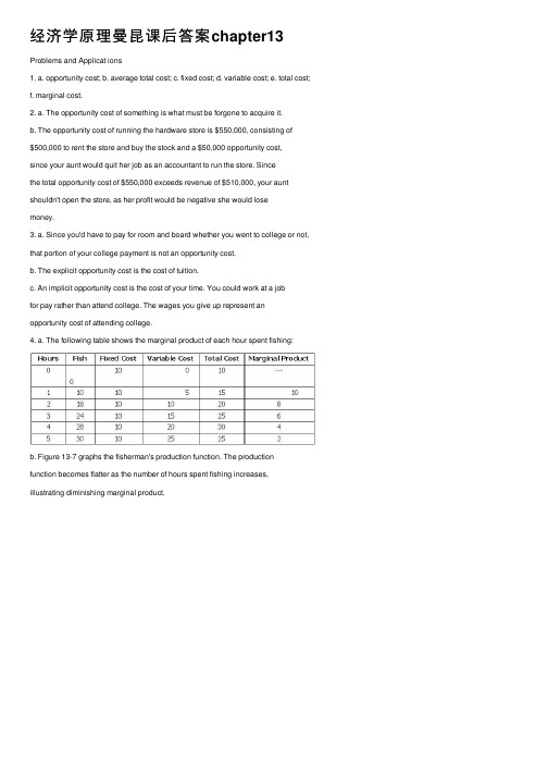
经济学原理曼昆课后答案chapter13 Problems and Applicat ions1. a. opportunity cost; b. average total cost; c. fixed cost; d. variable cost; e. total cost;f. marginal cost.2. a. The opportunity cost of something is what must be forgone to acquire it.b. The opportunity cost of running the hardware store is $550,000, consisting of $500,000 to rent the store and buy the stock and a $50,000 opportunity cost,since your aunt would quit her job as an accountant to run the store. Sincethe total opportunity cost of $550,000 exceeds revenue of $510,000, your aunt shouldn't open the store, as her profit would be negative she would losemoney.3. a. Since you'd have to pay for room and board whether you went to college or not, that portion of your college payment is not an opportunity cost.b. The explicit opportunity cost is the cost of tuition.c. An implicit opportunity cost is the cost of your time. You could work at a jobfor pay rather than attend college. The wages you give up represent an opportunity cost of attending college.4. a. The following table shows the marginal product of each hour spent fishing:b. Figure 13-7 graphs the fisherman's production function. The production function becomes flatter as the number of hours spent fishing increases, illustrating diminishing marginal product.Figure 13-7c. The table shows the fixed cost, variable cost, and total cost of fishing. Figure 13-8 shows the fisherman's total-cost curve. It slopes up because catching additional fish takes additional time. The curve is convex because there are diminishing returns to fishing time each additional hour spent fishing yields fewer additional fish.5. Here’s the table of costs:a. See table for marginal product. Marginal product rises at first, then declinesbecause of diminishing marginal product.b. See table for total cost.c. See table for average total cost. Average total cost is U-shaped. Whenquantity is low, average total cost declines as quantity rises; when quantity ishigh, average total cost rises as quantity rises.d. See table for marginal cost. Marginal cost is also U-shaped.e. When marginal product is rising, marginal cost is falling, and vice versa.f. When marginal cost is less than average total cost, average total cost is falling;when marginal cost is greater than average total cost, average total cost isrising.6. Fixed costs include the cost of owning or renting a car to deliver the bagels and thecost of advertising; they're fixed costs because they don't vary with output. Variable costs include the cost of the bagels and gas for the car, sincethose costs will increase as output increases.7. a. The fixed cost is 300, since fixed cost equals total cost minus variable cost. b.Marginal cost equals the change in total cost or the change in variable cost. That's because total cost equals variable cost plus fixed cost and fixed cost doesn't change as the quantity changes. So as quantity increases, the increase in total cost equals the increase in variable cost and both are equal to marginal cost.8. a. The fixed cost of setting up the lemonade stand is $200. The variable cost per cup is 50 cents.Figure 13-9b. The following table shows total cost, average total cost, and marginal cost. These are plotted in Figure 13-9.9. The following table illustrates average fixed cost (AFC), average variable cost (AVC), and average total cost (ATC) for each quantity. The efficient scale is 4 houses per month, since that minimizes average total cost.10. a. The following table shows average variable cost (AVC), average total cost (ATC), and marginal cost (MC) for each quantity.b. Figure 13-10 graphs the three curves. The margi nal cost curve is below the average total cost curve when output is less than 4, as average total cost is declining. The marginal cost curve is above the average total cost curvewhen output is above 4, as average total cost is rising. The marginal costcurve is always above the average variable cost curve, and average variablecost is always increasing.Figure 13-1011. The following table shows quantity (Q), total cost (TC), and average total cost (ATC)for the three firms:Firm A has economies of scale since average total cost declines as output increases.Firm B has diseconomies of scale since average total cost rises as output rises. Firm C has economies of scale for output from 1 to 3, then diseconomies of scale for greater levels of output.。
微观 曼昆经济学原理-课后答案
第一章经济学十大原理复习题4.为什么决策者应该考虑激励?答:因为人们会对激励做出反应。
如果政策改变了激励,它将使人们改变自己的行为,当决策者未能考虑到行为如何由于政策的原因而变化时,他们的政策往往会产生意想不到的效果。
6.市场中的那只“看不见的手”在做什么呢?答:市场中那只“看不见的手”就是商品价格,价格反映商品自身的价值和社会成本,市场中的企业和家庭在作出买卖决策时都要关注价格。
因此,他们也会不自觉地考虑自己行为的(社会)收益和成本。
从而,这只“看不见的手”指引着千百万个体决策者在大多数情况下使社会福利趋向最大化。
7.解释市场失灵的两个主要原因,并各举出一个例子。
答:市场失灵的主要原因是外部性和市场势力。
外部性是一个人的行为对旁观者福利的影响。
当一个人不完全承担(或享受)他的行为所造成的成本(或收益)时,就会产生外部性。
举例:如果一个人不承担他在公共场所吸烟的全部成本,他就会毫无顾忌地吸烟。
在这种情况下,政府可以通过制定禁止在公共场所吸烟的规章制度来增加经济福利。
市场势力是指一个人(或一小群人)不适当地影响市场价格的能力。
例如:某种商品的垄断生产者由于几乎不受市场竞争的影响,可以向消费者收取过高的垄断价格。
在这种情况下,规定垄断者收取的价格有可能提高经济效率。
9.什么是通货膨胀,什么引起了通货膨胀?答:通货膨胀是流通中货币量的增加而造成的货币贬值,由此产生经济生活中价格总水平上升。
货币量增长引起了通货膨胀。
10.短期中通货膨胀与失业如何相关?答:短期中通货膨胀与失业之间存在着权衡取舍,这是由于某些价格调整缓慢造成的。
政府为了抑制通货膨胀会减少流通中的货币量,人们可用于支出的货币数量减少了,但是商品价格在短期内是粘性的,仍居高不下,于是社会消费的商品和劳务量减少,消费量减少又引起企业解雇工人。
在短期内,对通货膨胀的抑制增加了失业量。
问题与应用7.社会保障制度为65岁以上的人提供收入。
如果一个社会保障的领取者决定去工作并赚一些钱,他(或她)所领到的社会保障津贴通常会减少。
- 1、下载文档前请自行甄别文档内容的完整性,平台不提供额外的编辑、内容补充、找答案等附加服务。
- 2、"仅部分预览"的文档,不可在线预览部分如存在完整性等问题,可反馈申请退款(可完整预览的文档不适用该条件!)。
- 3、如文档侵犯您的权益,请联系客服反馈,我们会尽快为您处理(人工客服工作时间:9:00-18:30)。
(一)单项选择题1 •总产量曲线的斜率是(C2. 当TP 下降时,(D )3. 当AP L 为正且递减时,MP L 是(A. 可变要素投入量的增长和产虽:的增长等幅变化B. 产量的增长幅度小于可变要素投入呈的增长幅度C. 可变要素投入量的增长幅度小于产量的增长幅度D 产量的增长幅度大于可变要素投入咼的增长幅度 5.某厂商每年从企业的总收入中取出一部分作为自己所提供的生产要素的报酬,这部分资金 被视为(B ).6•对应于边际报酬的递增阶段,STC 曲线(C )。
7•短期平均成本曲线成为U 形的原因与(C )有关 B.外部经济与不经济8•在从原点出发的射线与TC 曲线的相切的产量上,必有(D )o9. 如果生产10单位产品的总成本是100美元,第11单位产品的边际成本是21美元,那么扎第11单位产品TVC 是21美元B. 第10单位产品的边际成本是大于21美元C. 11个产品的平均成本是11美元 D 第12单位产品的平均成本是21美元 10.当边际成本小于平均成本时,产量的进一步增加将导致(B )。
A. 平均成本上升B. 平均可变成本可能上升也可能下降第13章生产和成本A.总产量B.平均产量C.边际产量D.以上都不是 A.AP L 递增 B.AP L 为零C.MK 为零D.MK 为负A.递减B.负的C.零D.以上任何一种4・生产过程中某一可变要素的收益递减,这意味着( B) A. 显性成本B. 隐性成本C. 经济利润D 生产成本A. 以递增的速率上升B. 以递增的速率下降C. 以递减的速率上升D 以递减的速率下降A.规模报酬 C.要素的边际报酬D 固立成本与可变成本所占比例A. AC 值最小B. AC=MCC.MC 曲线处于上升段D. A^ B 、C 、C.总成本下降D 平均可变成本一泄是处于减少的状态 11. 长期平均成本曲线呈U 型原因是(A )。
扎规模报酬的变化所致 B.外部经济与不经济所致C.生产要素的边际生产率所致 D 固泄成本与可变成本所占比重所致12. 如果一个厂商的生产是处于规模报酬不变的阶段,则其LAC 曲线一泄是处于(C )。
14. 下列说法中正确的是(D )扎生产要素的边际技术替代率是规模报酬递减造成的 B. 边际收益递减是规模报酬递减造成的 C. 规模报酬递减是边际收益递减规律造成的D 生产要素的边际技术替代率是边际收益递减规律造成的 15.当某厂商以最小成本生产既泄的产量时,该厂商(D )B. 一泄获得最大利润D 无法确左是否获得最大利润(二)简答题(这几个题目都很重要,没有写出答案的题目,请同学们请参考教材和课件) 1. 简述短期生产函数中总产量、平均产量及边际产量三者之间的关系。
2. 边际报酬递减规律的内容及成因。
3. 短期平均成本曲线和长期平均成本曲线都是U 型,请解释它们形成的原因有何不同? 短期平均成本曲线之所以呈U 型,是因为边际收益递减规律的作用。
具体地说,短期平均 成本之所以由下降转而上升,是因为AFC 的下降最终要被AVC 的上升所抵消,而AVC 的上 升是由可变要素的边际收益递减规律直接作用的结果。
然而,边际收益递减与长期平均成 本曲线的成因并没有直接的关系,因为在长期内没有任何固定的投入。
决定长期平均成本曲线形状的因素是规模收益的变动。
一般来说,在长期内,所有的要素 投入增加,企业规模扩大时,一开始是规模经济,随后会在一个或长或短的时期内规模收 益保持不变,然后随着产量的进一步增加,企业规模进一步扩大,会出现规模不经济。
规 模经济是指,产量增加的比例大于投入增加的比例,从而大于总成本增加的比例,这必然 导致平均成本的下降。
同样的原因当规模收益不变时,平均成本一定不变;当规模不经济 时,平均成本一定上升。
所以长期平均成本曲线扎上升趋势B.下降趋势13. 随着产量的增加,平均固泄成本将(D A. 保持不变C.水平状态D 垂直状态B. 开始时趋于下降,然后趋于上升扎总收益为零C. 一运未获得最大利润呈U型。
4.请分析为什么平均成本的最低点一左在平均可变成本的最低点的右边?平均成本是平均固定成本和平均可变成本之和。
当平均可变成本达到最低点开始上升时,平均固定成本一宜在下降,只要平均固定成本下降的幅度大于平均可变成本上升的幅度,平均成本就会继续下降,只有当平均可变成本上升的幅度和平均固定成本下降的幅度相等的时候,平均成本才达到最低点。
因此,平均总成本总是比平均可变成本晚到达最低点。
也就是说平均成本的最低点一定在平均可变成本的最低点的右边。
5.解释说明为什么在产量增加时,平均成本(AC)与可变成本(AVC)越来越接近?6.简述短期成本曲线之间的关系如何?(这是13章的关键内容,同学们参考课件)7.简述机会成本、显性成本、隐性成本、经济利润与会计利润之间的关系。
投入品的机会成本指因为使用这一资源而不得不放弃的其它利用场合可能带来的蜃彥的价值。
显性成本:要求企业支岀货币的投入成本,比如购买原材料的货款。
反应在财努报表中的。
从机会成本的角度讲,这些支岀的价格必须等于这些相同的生产要素使用在其它最好用途时所能得到的收入。
否则,这个企业就不能购买或租用到这些生产要素,并保持对他们的使用权。
隐性成本:不要求企业支岀货币的投入成本,不能够在会计账目中反应岀来的成本。
比如:投资者自己拥有的厂房的房租,投入资金的利息。
隐性成本也必须从机会成本的角度按照企业自有生产要素在其它最佳用途中所能得到的收入来支付,否则,厂商会把自由生产要素转移出本企业,以获得更髙的报酬。
显性成本+隐性成本二总机会成本经济利润二总收益■显性成本■隐性成本二总收益■总机会成本会计利润二总收益•显性成本会计利润总是大于经济利润。
厂商经济利润为零时,厂商还可以得到会计利润。
正常利润是指厂商对自己所提供的企业家才能的报酬的支付,正常利润是隐性成本的一个组成部分。
经济利润中不包括正常利润。
8 •当边际成本递增时,平均成本也是递增吗?当边际成本曲线递增时,平均成本曲线不一泄是递增的,也可能递减,如下图:当MC (边际成本)曲线到达最低点A以后,开始上升,在上升的初期,MC还是小于AC (平均成本),它不足以抵消整个平均成本的下降,平均成本还是下降的,直至达到AC的最低点B 点,此时MC等于AC,以后MC大于AC, AC开始随着MC的上升而上升。
所以当MC曲线增加的时候AC曲线先下降,当达到最低点以后开始上升。
请大家记住的就是当MC小于AC时, AC就是递减的;当MC大于AC时,AC就是递增的。
不需看MC是递増还是递减。
(三)分析计算题1 •已知生产函数为 Q二f (K, L )=KL - 0. 5L: - 0. 32K\ 若 K二 10」(1)求AP L和MK函数;⑵求AP L最大化时厂商雇佣的劳动。
解:(1)把 K二 10 代入生产函数 Q二f (K, L )=KL - 0. 5L2 - 0. 32K3 可得0 = 10厶一0・5厶2一32。
g=10L-0.5L--32=1()_05L_32L L LMP, = 乂 =哎=0 (厶)=(10厶一 O.5L 2 一 32) J 10 — 厶AL dL(2)当AP L =MP L 时,达到最大。
在两者相等之前4仇是递增的,相等之后A&开 始递减。
32 3210 — 0.5厶 =10 — L => 0.5L = — => L 2= 64 => L = ±8L LL = -8舍去,所以L = &可得最大时,L 二8。
2. 假设某企业的短期成本函数是TC (Q) =Q 3-10Q :+170Q-66 (1) 指出该短期成本函数中的可变成本部分和不变成本部分:(2) 写出下列相应的函数:TVC (Q), AC (Q), AVC (Q) AFC (Q)和 MC (Q 〉° 解(1)可变成本部分:VC = 03—1002+1700不变成本部分:FC = 66 (2) TVC(Q)=Q 3-\0Q 2+H0QMC = TC(Q) = (03—1002+1700 + 66)'= 302-200 + 170s£MC = VC(C) =(e 3-10(22+l700'= 302 一 20Q +1703. 已知某厂商的短期总成本函数是STC (Q)二0. 01Q 5-0. 8Q :+10Q+5,求最小的平均可变成本值。
解:当= 寸,UC 达到最小。
AC(Q) = TC(Q) Q03-1OQ2+17OQ + 66Q=Q 2 — 10Q + 170 +詈AVC =VC03-1002+1700Q= 02—100 + 170AFC =FC 66所以当(2 = 10时,平均可变成本最小 此时VC MIN = 0.04X10³-0.8X10²+10X10 = 64. 设某个生产者的生产函数为Q 二已知K 二4,貝总值为100, L 的价格为10。
求 (1) L 的投入函数和生产Q 的总成本函数、平均成本函数和边际成本函数; (2) 如果Q 的价格为40,生产者为了获得最大利润应生产多少Q 能获得多少利润:⑶如果K 的总值从100上升120, Q 的价格为40,生产者为了获得最大利润应生产Q 能获 得多少利润。
Q = \l KL =、/4 厶=> L = ^―TC = KP K =100+10L = 100+10X ^- = 100+|(22MC = TC= (100+-e 2) = 502K = 77?_TC = P X 0_(1OO + ?Q2)= 400 — 100-2022 2⑵ 於=(400- 100-?0今=40-50 = 0 = 0 = &此时生产者获得最大利闰。
^x = 40x8-120-|x82=40Q 2 = 0(舍去)解:(1)Q QMC = STC (0 = (0.0403-0.8(22 +100 + 5),= 0.1202 -1.6(3 + 10AC = — = ------ = -- = —Q 4 --Q Q 2 Q。