comsol模拟电机旋转-磁场
COMSOL-Multiphysics中2D非线性磁场有限元仿真
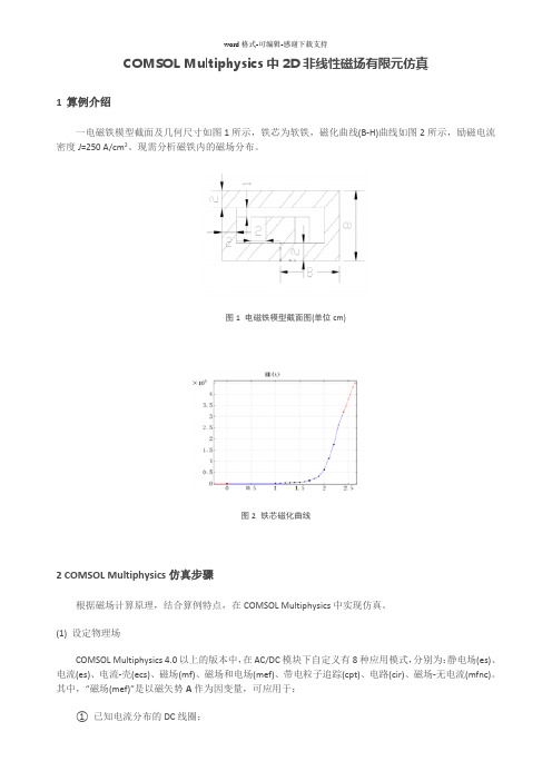
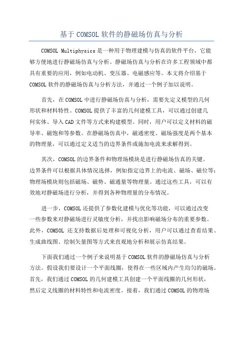
COMSOL Multiphysics中2D非线性磁场有限元仿真1算例介绍一电磁铁模型截面及几何尺寸如图1所示,铁芯为软铁,磁化曲线(B-H)曲线如图2所示,励磁电流密度J=250 A/cm2。
现需分析磁铁内的磁场分布。
图1电磁铁模型截面图(单位cm)图2铁芯磁化曲线2 COMSOL Multiphysics仿真步骤根据磁场计算原理,结合算例特点,在COMSOL Multiphysics中实现仿真。
(1)设定物理场COMSOL Multiphysics 4.0以上的版本中,在AC/DC模块下自定义有8种应用模式,分别为:静电场(es)、电流(es)、电流-壳(ecs)、磁场(mf)、磁场和电场(mef)、带电粒子追踪(cpt)、电路(cir)、磁场-无电流(mfnc)。
其中,“磁场(mef)”是以磁矢势A作为因变量,可应用于:①已知电流分布的DC线圈;②电流趋于表面的高频AC线圈;③任意时变电流下的电场和磁场分布;根据所要解决的问题的特点——分析磁铁在线圈通电情况下的电磁场分布,选择2维“磁场(mf)”应用模式,稳态求解类型。
(2)建立几何模型根据图1,在COMSOL Multiphysics中建立等比例的几何模型,如图3所示。
图3几何模型有限元仿真是针对封闭区域,因此在磁铁外添加空气域,包围磁铁。
由于磁铁的磁导率,因此空气域的外轮廓线可以理想地认为与磁场线迹线重合,并设为磁位的参考点,即(21)式中,L为空气外边界。
(3)设置分析条件①材料属性本算例中涉及到的材料有空气和磁铁,在软件自带的材料库中选取Air和Soft Iron。
对于磁铁的B-H曲线,在该节点下将已定义的离散B-H曲线表单导入其中即可。
②边界条件由于磁铁的磁导率,因此空气域的外轮廓线可以理想地认为与磁场线迹线重合,并设为磁位的参考点,即(21)式中,L为空气外边界。
为引入磁铁的B-H曲线,除在材料属性节点下导入B-H表单之外,还需在“磁场(mef)”节点下选择“安培定律”,域为“2”,即磁铁区域,在“磁场>本构关系”处将本构关系选择为“H-B曲线”。
基于COMSOL Multiphysics的磁场仿真分析

[1]]● 宋 J 浩 ,黄彦1j,邓 志扬 ,等.几 组 特殊 形 1{ 状 永磁 体 的磁 ] J
场及梯度 COMSOL分 析 [J].大学物 理实验 ,2013, 26(4):3-7. 刘 延 东 ,徐 志 远 .基 于 Comsol Multiphysics无 限 长 圆 柱载流导线产生 的磁场分 布研究 [J].现代 电子技 术 ,2015,38(2):9.14. 王慧娟 ,李慧奇 .基 于仿 真 软件 的电磁 场实验教 学 研究 [J].大学物理实验 ,2015,28(1):79-81. 郭 硕 鸿.电 动 力 学 [M].北 京 :高 等 教 育 出 版 社 ,2008. 郑晶晶.基于 Comsol电磁器件 的设计 与仿 真 [D]. 南昌 :南 昌大学 ,2014. 梁灿彬 ,秦光戎 ,梁竹健 .电磁学 [M].北京 :高等 教 育出版社 ,2004. 黄 昆.固 体 物 理 学 [M].北 京 :高 等 教 育 出 版 社 .1988. 张裕 恒.超 导物 理 [M].合肥 :中 国科 学 技术 出 版 社 ,2009. 金桂 ,姚敏 ,蒋纯志.大学物理演示实 验教学探索 与 实践 [J].大学物理实验 ,2015,35(4):113—115.
t0r in the external magnetic f ield.Finally.br ief ly ana lyzed these magnetic f ields. Key words:COMSOL;per m anent magnet;superconductor;distr ibution of mag n etic f ield
基于 COMSOL Multiphysics的磁场仿真分析
场 ,而是其 自身产生 的磁场与外磁场方向相反最 终 导致 磁感应 强度 为零 j。
基于COMSOL软件的静磁场仿真与分析
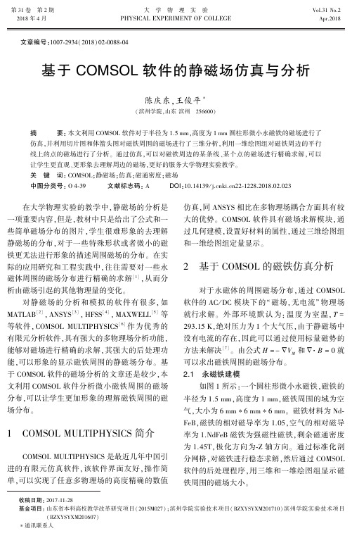
第31卷第2期大学物理实验Vol.31No.22018年4月PHYSICALEXPERIMENTOFCOLLEGEApr.2018收稿日期:2017 ̄11 ̄28基金项目:山东省本科高校教学改革研究项目(2015M027)ꎻ滨州学院实验技术项目(BZXYSYXM201710)滨州学院实验技术项目(BZXYSYXM201607)∗通讯联系人文章编号:1007 ̄2934(2018)02 ̄0088 ̄04基于COMSOL软件的静磁场仿真与分析陈庆东ꎬ王俊平∗(滨州学院ꎬ山东滨州㊀256600)摘要:本文利用COMSOL软件对于半径为1.5mmꎬ高度为1mm圆柱形微小永磁铁的磁场进行了仿真ꎬ并利用切片图和体箭头图对磁铁周围的磁场进行了三维分析ꎬ利用一维绘图组对磁铁周边的平行线上的点的磁场进行了分析ꎮ通过仿真ꎬ可以对磁铁周边的某条线㊁某个点的磁场进行精确求解ꎬ可以让学生更直观㊁更形象去理解周边的磁场ꎬ更好的服务大学物理实验教学ꎮ关键词:COMSOLꎻ静磁场ꎻ仿真ꎻ磁通密度ꎻ磁场中图分类号:O4 ̄39文献标志码:ADOI:10.14139/j.cnki.cn22 ̄1228.2018.02.023㊀㊀在大学物理实验的教学中ꎬ静磁场的分析是一项重要内容ꎬ但是ꎬ教材中只是给出了公式和一些简单磁场分布的图片ꎬ学生很难形象的去理解静磁场的分布ꎬ对于一些特殊形状或者微小的磁铁更无法进行形象的描述周围磁场的分布ꎮ在实际的应用研究和工程实践中ꎬ往往需要对一些永磁体周围的磁场分布进行精确的求解[1]ꎬ从而分析由磁场引起的其他物理量的变化ꎮ对静磁场的分析和模拟的软件有很多ꎬ如MATLAB[2]ꎬANSYS[3]ꎬHFSS[4]ꎬMAXWELL[5]等等软件ꎬCOMSOLMULTIPHYSICS[6]作为优秀的有限元分析软件ꎬ具有强大的多物理场分析功能ꎬ能够对磁场进行精确的求解ꎬ其强大的后处理功能ꎬ可以形象的显示磁铁周围的静磁场分布ꎮ基于COMSOL软件的磁场分析的文章还是较少ꎬ本文利用COMSOL软件分析微小磁铁周围的磁场分布ꎬ可以让学生更加形象的理解磁铁周围的磁场分布ꎮ1㊀COMSOLMULTIPHYSICS简介COMSOLMULTIPHYSICS是最近几年中国引进的有限元仿真软件ꎬ该软件界面友好ꎬ操作简单ꎬ可以实现了任意多物理场的高度精确的数值仿真ꎬ同ANSYS相比在多物理场耦合方面具有较大的优势ꎮCOMSOL软件具有磁场求解模块ꎬ通过几何建模ꎬ设置好材料的属性ꎬ通过三维绘图组和一维绘图组定量显示ꎮ2㊀基于COMSOL的磁铁仿真分析对于永磁体的周围磁场分布ꎬ通过COMSOL软件的AC/DC模块下的 磁场ꎬ无电流 物理场就行求解ꎮ外部环境默认为:温度为室温ꎬT=293.15Kꎬ绝对压力为1个大气压ꎬ由于静磁场中没有电流的存在ꎬ因此可以通过使用标量磁势的方法来解决[7]ꎮ由公式H=-ÑVM和Ñ B=0就可以求出磁铁周围的磁场分布ꎮ2.1㊀永磁铁建模如图1所示:一个圆柱形微小永磁铁ꎬ磁铁的半径为1.5mmꎬ高度为1mmꎬ磁铁周围的域为空气ꎬ大小为6mm∗6mm∗6mmꎮ磁铁材料为Nd ̄FeBꎬ磁铁的相对磁导率为1.05ꎬ空气的相对磁导率为1.NdFeB磁铁为强磁性磁铁ꎬ剩余磁通密度为1.45Tꎬ极化方向为 ̄Z轴方向ꎮ通过标准化剖分网格ꎬ对磁铁进行稳态求解ꎬ然后通过COMSOL软件的后处理程序ꎬ用三维和一维绘图组显示磁铁周围的磁场大小ꎮ图1㊀永磁体建模结构图2.2 永磁铁周围磁场分析对于半径为1.5mmꎬ高度为1mm圆柱形微小永磁铁ꎬ磁铁周围的磁场很难准确测量ꎬ通过COMSOL软件可以定量的显示周围的磁场ꎮCOMSOL软件结果后处理程序有三维绘图组和一维绘图组ꎬ本文分别从三维和一维绘图组定量显示微小磁铁周边的磁场ꎮ图2为磁铁周围磁场的三维绘图组中的切片图ꎬ图中水平切片图为距离磁铁底部0.1mm的xy平面切片图ꎬ从中可以看出ꎬ磁铁圆周两侧的磁通密度最大ꎬ磁场最强ꎬ从圆周往外和向圆心方向均逐渐减小ꎬ面上的磁通密度最大值为0.61Tꎬ最小0.05Tꎻ图中竖直切片图为距离磁铁圆心1.6mm即距离磁铁边缘0.1mm的yz平面切片图ꎬ从切面图上可以看出ꎬ磁铁的上下面与yz切面相交的位置磁场最强ꎬ远离磁铁边缘的点逐渐减小ꎬ面上的磁通密度最大值为0.632Tꎬ最小0.007Tꎮxy和yz切面的位置可以任意设定ꎬ可以查看求解空气域里任意位置的切面图ꎬ也可以同时查看多个平行或相交的切面图ꎮ图2㊀永磁体周围磁场的切片图图3为永磁体周围磁场的体箭头图ꎬ体箭头的疏密和颜色的深浅代表此处磁通密度的大小ꎬ体箭头的方向代表磁场的方向ꎬ从图中可以看出ꎬ磁力线从 ̄Z轴方向起始ꎬ轴向绕磁铁一周ꎬ从Z轴方向终止ꎬ和理论上一致ꎮ从侧面(a)和正面(b)图中可以看出ꎬ磁场最强的位置就位于磁力线走向的位置即磁铁上下面的圆周边缘及轴向绕磁铁一周的位置ꎬ磁铁极化方向的下表面的磁场强度大于上表面ꎬ远离磁铁的位置ꎬ磁场逐渐减小ꎮ图3㊀永磁体周围磁场的体箭头图98基于COMSOL软件的静磁场仿真与分析㊀㊀为了更好的定量显示磁铁周围的磁场分布ꎬ可以制作一维绘图组ꎬ这样ꎬ就可以显示每个点上的磁感应强度ꎬCOMSOL软件可以做求解域里的任意三维截线ꎬ为此ꎬ在 ̄Z轴上距离Z轴原点中心不同距离做了一组三维截线ꎬ距离分别为-0.2ꎬ-0.3.-0.5ꎬ-0.8.-1mmꎬꎬ图4中的(a)图为距离-0.5mm的三维截线ꎬ这五条截线X坐标从-3mm到3mmꎬY坐标为0ꎬ根据这五条三维截线ꎬ做了截线上各点磁通密度模的一维绘图组ꎬ图4中的(b)图为 ̄Z轴上距离原点中心不同距离X轴平行线上各点磁通密度模ꎬ从图中可以看出ꎬ由于磁铁的半径是1.5mmꎬ磁场在磁铁边缘处变化率最大ꎬ磁铁变化率大的位置如果磁铁运动ꎬ产生的感应电动势就大ꎻ距离磁铁很近的位置ꎬ0.2mm的平行线ꎬ从磁铁的边缘到磁铁的中心位置ꎬ磁场逐渐减小ꎬ当距离磁铁较远的位置0.5mmꎬ0.8mm这种现象就消失了ꎬ磁场从边缘到中心基本相等ꎬ磁铁变化率最大的位置仍为磁铁边缘ꎮ图4㊀ ̄Z轴上距离原点中心不同距离X轴平行线上各点磁通密度模图5㊀X轴上距离原点中心不同距离Z轴平行线上各点磁通密度模09基于COMSOL软件的静磁场仿真与分析㊀㊀同样ꎬ在X轴上距离X轴原点中心不同距离做了一组三维截线ꎬ距离分别为1.6ꎬ1.8.2ꎬ2.5ꎬ3mmꎬ图5中的(a)图为距离1.8mm的三维截线ꎬ这五条截线Z坐标从-3mm到3mmꎬY坐标为0ꎬ根据这五条三维截线ꎬ做了截线上各点磁通密度模的一维绘图组ꎬ图5中的(b)图为X轴上距离原点中心不同距离Z轴平行线上各点磁通密度模ꎬ从图中可以看出ꎬ由于磁铁的高度是1mmꎬ磁场在磁铁上下边缘处变化率最大ꎬ即Z坐标在0和1mm处ꎬ此两处产生的感应电动势就大ꎻ距离磁铁很近的位置ꎬ0.1mm的平行线ꎬ从磁铁的边缘到磁铁的中心位置ꎬ磁场逐渐减小ꎬ当距离磁铁较远的位置0.3mmꎬ0.5mm这种现象就消失了ꎬ磁场从边缘到中心基本相等ꎬ磁铁变化率最大的位置仍为磁铁上下边缘ꎮ3㊀结㊀语本文利用COMSOL软件对于半径为1.5mmꎬ高度为1mm圆柱形微小永磁铁的磁场进行了仿真ꎬ并利用切片图和体箭头图对磁铁周围的磁场进行了三维分析ꎬ利用一维绘图组对磁铁周边的平行线上的点的磁场进行了分析ꎮ通过分析ꎬ可以看出ꎬ利用COMSOL软件可以直观的㊁定量的对磁铁的周边的某一个切面ꎬ某一个平行线的磁场进行显示ꎬ特别是一些特殊形状磁铁ꎬ或者是磁铁组合的磁场分析ꎬ这些仿真处理方法具有重要意义ꎮ利用COMSOL软件对磁铁周围的磁场进行仿真分析ꎬ可以让学生更直观的去理解周边的磁场ꎬ更好的服务大学物理实验教学ꎮ参考文献:[1]㊀宋浩ꎬ黄彦ꎬ邓志扬ꎬ等.几组特殊形状永磁体的磁场及梯度COMSOL分析[J].大学物理实验ꎬ2013ꎬ26(4):3 ̄7.[2]㊀李晶晶.基于matlab与comsol的磁场仿真研究[D].吉林:吉林大学:2015.[3]㊀王月明ꎬ刘官元ꎬ杨友松.基于有限元ANSYS的圆线圈磁场仿真研究[J].内蒙古科技大学学报ꎬ2011ꎬ30(1):94 ̄96.[4]㊀屈乐乐ꎬ杨天虹ꎬ胡爱玲ꎬ等.基于HFSS的微波器件仿真实验设计与应用[J].实验室研究与探索ꎬ2017ꎬ36(3):86 ̄89.[5]㊀陈红ꎬ侯国栋.长直螺线管的电磁场分析与仿真[J].郑州轻工业学院学报ꎬ2013ꎬ28(1):100 ̄104.[6]㊀吕琼莹ꎬ杨艳ꎬ焦海坤ꎬ等.基于comsolmultiphysics超声波电机的谐振特性分析[J].压电与声光ꎬ2012ꎬ34(6):864 ̄867.[7]㊀郭硕鸿.电动力学[M].北京:高等教育出版社ꎬ2008.SimulationandAnalysisofMagnetostaticFieldbasedonCOMSOLSoftwareCHENQing ̄dongꎬWANGJun ̄ping∗(BinzhouUniversityꎬShandongBinzhou256600)Abstract:Themagneticfieldoftheradiusof1.5mmandheightof1mmmicrocylindricalpermanentmagnetissimulatedbyCOMSOLsoftwareꎬthe3Dmagneticfieldisanalyzedbyslicemapandvolumearrowdiagramꎬthepointofparallellinessurroundingofthemagnetisanalyzedbyonedimensionaldrawinggroup.Throughsimulationꎬthemagneticfieldofalineorapointaroundamagnetcanbesolvedaccuratelyꎬwhichcanmakestudentsmoreintuitiveandmorevividtounderstandthesurroundingmagneticfieldꎬandbetterservetheteach ̄ingofcollegephysicsexperiment.Keywords:COMSOLꎻmagnetostaticꎻsimulationꎻdensityofmagneticfluxꎻmagneticfield19基于COMSOL软件的静磁场仿真与分析。
基于亥姆霍兹线圈的旋转磁场设计方法和COMSOL 有限元仿真
科技与创新┃Science and Technology &Innovation·46·2019年第06期文章编号:2095-6835(2019)06-0046-03基于亥姆霍兹线圈的旋转磁场设计方法和COMSOL 有限元仿真范程颖(同济大学,上海200000)摘要:首先提出了旋转磁场的数学描述,然后介绍了基于三维亥姆霍兹线圈的旋转磁场实现,最后基于COMSOL 有限元分析软件对三维亥姆霍兹旋转磁场做了仿真分析。
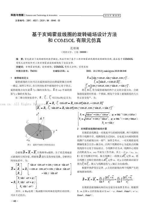
关键词:亥姆霍兹线圈;旋转磁场;COMSOL 有限元分析;空间坐标中图分类号:TM301文献标识码:ADOI :10.15913/ki.kjycx.2019.06.0461旋转磁场定义旋转磁场的方向可以由旋转面的法向即旋转轴方向唯一确定,如图1所示,在空间坐标系中磁场的中心处于原点,旋转磁场方向矢量n 与z 轴的夹角为γ,n在xoy 平面的投影与x 轴的夹角为α.在三维空间坐标系中,n,1l ,2l 可以由α和γ定义为:.]cos sin sin cos [sin T γαγαγ,,=n.]0cos [sin T 1,,αα-=l .]sin sin cos cos [cos T 2γαγαγ-=,,l 将1l 和2l 作为旋转磁场的两个正交的分量方向,合磁场强度旋转时形成一个圆面,则每个分量上磁场强度的大小作正弦变化[1],为:.]sin sin cos cos [cos sin sin ]0cos [sin cos cos T0202T0101⎪⎩⎪⎨⎧-=⋅⋅=-=⋅⋅=γαγαγωωααωω,,,,t B t l B B t B t l B B 图1旋转平面的空间坐标表示合磁场12B B B =+以角频率ω旋转,为了更直观地显示磁场的空间分量,将磁场B进行直角坐标变换,分解到空间坐标系中,为:.sin sin sin sin sin sin sin cos cos cos sin cos cos cos sin k j j i i 00z y x ⎥⎥⎥⎦⎤⎢⎢⎢⎣⎡++=⎥⎥⎥⎦⎤⎢⎢⎢⎣⎡⋅-⋅+⋅-⋅+⋅=⎥⎥⎥⎦⎤⎢⎢⎢⎣⎡=)()()(t k t k t k B t t t t t B B B B B ωϕωϕωωγωαγωαωαγωα其中,k 和φ是将三角函数中间项和差化积后的结果,可由下式给出:.sin tan cos tan sin cos cos cot cos tan cos cos sin k 1i 222j 1i222i ⎪⎪⎩⎪⎪⎨⎧-=-=+==+=--γαγϕαγααγϕαγαk k k )(,)(,2亥姆霍兹线圈的磁场计算亥姆霍兹线圈是一对彼此平行的相同线圈,两个线圈间距等于线圈半径,线圈绕线方式同向,且电流方向相同使得线圈产生的磁场方向一致[2]。
基于COMSOL旋转机械电机的电力电磁耦合分析
H
用 具 有 相 同相 对 磁导 率 的材 料 ,将 磁 场 局 限 于 闭
收 稿 日 期 :2 1- 6 2 02 0- 6
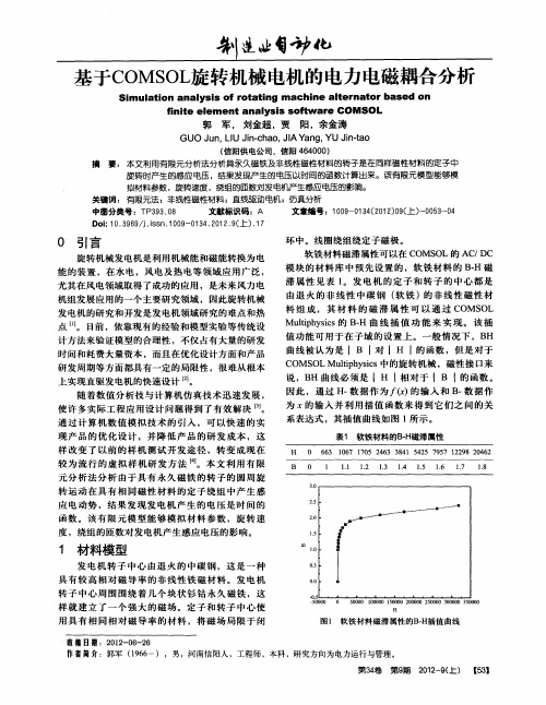
图 1 软 铁 材 料 磁 滞 属 性 的 B H 值 曲线 —插
作者简介:郭军 (9 6 16 一),男 ,河南信阳人 ,工程 师,本科 ,研究方向为电力运行与管理 。 第3 卷 第9 4 期 2 1 — ( ) [3 o2 9上 51
【】J r my Elo ,Le sGio ,De o a ti F ne 2 ee s n wi r d b r h Esrn. i —
gr i e N ew o k m e Syn hr i ai sng Re e e e a n d t r Ti c on z ton U i f r nc
1 . 01
I E 8 2 1 . P a ol r i ls S n o ew r s / E E 0 . 4 l fr l o r es e s r t o k [ / 5 t Tf W e N C]
Pr c. 00 o of2 6.I EEE n e a ina I t r to lCon e e e o yse s n f r nc n S t m , M a nd Cy r e cs n a be n t .Taie ,Tawa i pi i n,Ch n i a:I EEE e s Pr s , 2 6. 0o
系表 达式 ,其插 值 曲线如 图 1 示 。 所
表 1 软铁材料的B H — 磁滞属性
H 0 6 3 1 6 1 0 2 63 8 5 2 7 5 1 2 8 2 4 2 6 0 7 7 5 4 3 41 4 5 9 7 2 9 O 6
comsolmultiphysics精典实例直线电机建模仿真

模型描述 – 方程
在二维问题中,COMSOL利用磁势A的静磁方程求解该问题
01r1Az 0 0 1 1 rr 1 1B BrryxJze
结果
Z分量的电势分布
感 谢
COMSOL AC/DC模块培训
主讲人: 上海中仿科技
利用COMSOL计算直线电机
直线电机是一种不用其他装置就能产生直线运动的 电机设备。沿半径方向把旋转电机的定子和转子切开,产 生一个直线推力,就成了直线电机。
AC/DC_Module/Motors_and_Drives/coil_LEM
模型描述 –几何
基于COMSOL软件的静磁场仿真与分析
基于COMSOL软件的静磁场仿真与分析COMSOL Multiphysics是一种用于物理建模与仿真的软件平台,它能够方便地进行静磁场仿真与分析。
静磁场仿真与分析在许多工程领域中都具有重要的应用,例如电动机、变压器、电磁感应等。
本文将介绍基于COMSOL软件的静磁场仿真与分析方法,并通过一个例子加以说明。
首先,在COMSOL中进行静磁场仿真与分析,需要先定义模型的几何形状和材料特性。
COMSOL提供了丰富的几何建模工具,可以通过创建几何实体、导入CAD文件等方式来构建模型。
同时,用户可以定义材料的磁导率、磁饱和等参数。
在静磁场仿真中,磁通密度、磁场强度是两个基本的物理量,可以通过定义适当的边界条件或施加电流来求解得到。
其次,COMSOL的边界条件和物理场模块是进行静磁场仿真的关键。
边界条件可以根据具体情况选择,例如指定边界上的电流、磁场、磁位等;物理场模块则包括磁场、磁势、磁通量等物理量。
通过这些工具,可以有效地对静磁场进行分析,并得到各种物理量的分布情况。
进一步,COMSOL还提供了参数化建模与优化等功能,可以通过改变一些参数来对静磁场进行灵敏度分析,并找出影响磁场分布的重要参数。
此外,COMSOL还支持数据后处理和可视化分析,用户可以通过查看结果、生成曲线图、绘制矢量图等方式来直观地分析和展示仿真结果。
下面我们通过一个例子来说明基于COMSOL软件的静磁场仿真与分析方法。
假设我们要设计一个平面线圈,使得在一些区域内产生均匀的磁场。
首先,我们通过COMSOL的几何建模工具创建一个平面线圈的几何形状,然后定义线圈的材料特性和电流密度。
接着,我们通过COMSOL的物理场模块求解得到平面线圈中的磁场分布,并利用COMSOL的后处理工具进行分析和展示。
在仿真结果中,我们可以观察到平面线圈中磁场的分布情况,包括磁场强度、磁通密度等。
我们可以通过改变线圈的几何形状、电流密度等参数,来研究对磁场分布的影响。
使用COMSOL分析各类旋转机械

使用COMSOL分析各类旋转机械在模拟旋转机械时,可以通过研究振动对机器性能的影响来有效避免机器故障。
为了实现这一目标,一种方法是使用新的“转子动力学模块”,它是 COMSOL Multiphysics® 软件“结构力学模块”的扩展模块。
在本文中,我们将介绍“转子动力学模块”,带领你了解它的实用特征和功能,助你改进旋转机械设计流程。
转子动力学建模有哪些用途?首先,我们简要介绍一下转子动力学建模。
如之前发布的一篇文章所述,旋转机械具有广泛的应用,从航空航天技术到发电,遍及众多行业,转子动力学分析十分有助于加强旋转机械的功能,提高安全性。
举例来说,假设你要确保一台发电机(一种旋转机械)避免由设计欠佳导致的不稳定、破坏性共振和故障问题。
这时你可以执行转子动力学分析,研究影响发电机物理特性的振动现象,以及由发电机的旋转和结构引起的振动加剧。
发电机(左)及其三维模型(右)。
借助仿真软件,你能够提高转子动力学研究的准确性和简易性。
现在,加上“转子动力学模块”,这一过程会变得更加方便灵活。
“转子动力学模块”会帮助你设置正确的设计参数,分析共振、应力、应变以及横向和扭转振动效应对旋转机械的的影响,由此使响应保持在可接受的运行限制范围内。
此外,你能进一步了解固定和移动的转子组件如何影响产品设计,并计算临界速度、固有频率和振型。
在下一节中,我们将深入探讨一些具体的优点和功能。
为什么要使用“转子动力学模块”?“转子动力学模块”的突出优势之一是其出色的灵活性。
你可以轻松地自定义仿真分析,方便地研究旋转装配或整个结构的特定组成部分。
上述操作的第二项可通过“转子动力学模块”的实心转子接口来实现,在有限元建模中,此接口使用三维 CAD 几何表示转子和实体单元。
你可以通过研究旋转装配中的所有组件来生成最精确的结果。
在分析转子的应力和变形时,你不需要去模拟整个系统,这样会提高仿真的精度。
为了计算整个域中的应力分布和变形场分布,你必须将转子模拟为实心单元。
基于有限元方法模拟电机旋转磁场
t er ai ft e f r r / e es lr tt n o h lcrc 1ma h n g ei il h e l y o h o wa d rv r a o a i ft e ee tia c i e ma n t f d,a d t e n tae t o c e n o d mo s r t
Ab ta t I hi a e ,The a t a sr c :n t s p p r c u lmov me tofm a e n gne i i l n t e — tcfe d i hr e pha e a t r tng c r n a hi e s le na i ur e tm c n s i n l e y t e fn t l me t me h . The smul to e ul s p o e o be a e t e c i e pe f c l s a a yz d b h i ie e e n t od i a i n r s ti r v n t bl o d s rb r e ty
第 3 3卷
第 2期
电气 电子 教 学 学 报 J OuRNAL OF E EE
Vo1 3 NO 2 . 3 . AD . Ol r2 1
2 1 年 4月 01
基 于 有 限 元 方 法 模 拟 电机 旋 转 磁 场
郭 健
( 南京 航 空航 天 大 学 自动 化 学 院 , 苏 南京 2 0 1 ) 江 1 0 6
限元模 型 。
进行 描述 , 学生 也难 于理解 , 致使 这部 分 内容 的教 学
效果 普遍 较差口 ] 。本 文 采 用有 限元 的方法 对 三 相
交 流 电机 内部 磁 场 的实 际 运 动 情 况进 行 了模 拟 仿
COMSOL 4.4 模拟螺线管线圈产生的磁场分布
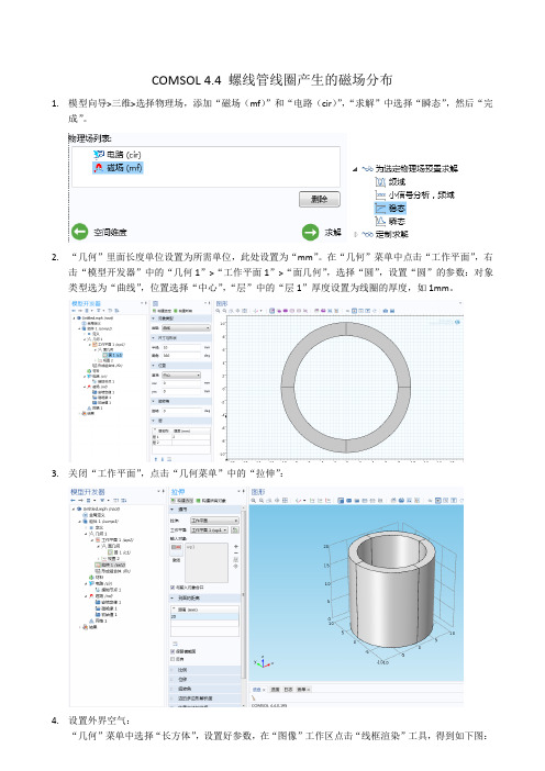
COMSOL 4.4 螺线管线圈产生的磁场分布1.模型向导>三维>选择物理场,添加“磁场(mf)”和“电路(cir)”,“求解”中选择“瞬态”,然后“完成”。
2.“几何”里面长度单位设置为所需单位,此处设置为“mm”。
在“几何”菜单中点击“工作平面”,右击“模型开发器”中的“几何1”>“工作平面1”>“面几何”,选择“圆”,设置“圆”的参数:对象类型选为“曲线”,位置选择“中心”,“层”中的“层1”厚度设置为线圈的厚度,如1mm。
3.关闭“工作平面”,点击“几何菜单”中的“拉伸”:4.设置外界空气:“几何”菜单中选择“长方体”,设置好参数,在“图像”工作区点击“线框渲染”工具,得到如下图:5.右击“模型开发器”中的“定义”>“视图1”,选择“隐藏几何实体”,在“隐藏几何实体”编辑区,选择“几何实体层次”中的“边界”,手动选择需要隐藏的边界:长方体的六个面,则可以得到下图:6.定义各个域和边界:定义线圈:点击“定义”菜单栏中的“显示”,“模型开发器”中的“定义”下面会出现“显示1”,右击并重命名为“线圈”,然后在“显示”工作区将“几何实体层次”选择为“域”,再选择图中看到的圆筒,此时圆筒有四个域,由于圆筒与后来的长方体重合,所以长方体现在变成了“域1”,而圆筒变成了“域2,3,4,5”:定义线圈边界:同样的方法在“定义”中得到“显示2”,并重命名为“线圈边界”,在“显示”编辑区的“几何实体层次”中选择“边界”,并在图形中选择圆筒的各个边界,此时圆筒中的四个域中接触面也算一个边界。
本例中可以在“显示”编辑区点击“粘贴选择”按钮,输入“7-14,16-19,21-14”,点击“确认”。
定义空气:同样的方法,选择“域1”位空气,就是刚刚建立的长方体,此时空气的边界已被隐藏,所以此处看不见长方体。
7.设置“磁场(mf)”:设置“多匝线圈1”:右击“模型开发器”中的“磁场(mf)”,选择“多匝线圈”,在“多匝线圈”编辑区的“域选择”栏选择刚刚定义的“线圈”,“线圈类型”栏选择“数值”,“多匝线圈”栏中的“匝数”N设置为所需数字,如100,“线圈激励”中选择“电路(电流)”。
COMSOL中的二维发电机仿真
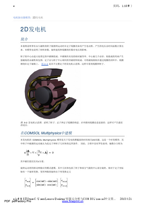
电机驱动器模型:2D发电机2D发电机简介本案例说明带有永久磁铁的转子做圆周运动时在定子线圈内如何产生电动势。
产生的电压由时间函数计算出来。
本模型也说明了材料参数,旋转速度和线圈的匝数对电压的影响。
转子的中心由退火处理过的中碳钢组成,中碳钢具有高的相对磁导率。
中心被几个由钐,钴做成的用来产生强磁场的永磁铁块包围。
定子由与转子中心相同的导磁材料制成,可将磁场限制在通过线圈的闭环中。
线圈缠绕在定子磁极上。
图 3-2是具不完整定子的发电机示意图,这样可看到线圈和转子。
图3-2: 发电机示意图,说明了转子,定子和定子线圈的构造。
在环路间线圈也是连接的,这样可产生最高的电压。
在COMSOL Multiphysics中建模本发电机的COMSOL Multiphysics 模型是关于发电机横截面的时间相关2D问题。
这是一个时变模型,其中转子中磁源的运动被认为是定子和转子几何体的边界条件。
因此,方程中没有罗伦兹项,偏微分方程为其中磁位能仅仅有z分量。
旋转运动利用移动网格应用模式建模,其中几何体包括了转子和部分气隙的中心部分旋转,相对于定子坐标轴有一个旋转变换。
变形网格的旋转由下列变换定义转子和定子是两个分离的几何对象,因此可使用装配几何体(详见COMSOL Multiphysics Modeling Guide413页的“使用装配” )。
这样有几个好处:转子和定子可自动耦合,部件可单独划分网格,并且允许两个几何体界面(称为裂缝)上的位能矢量不连续。
转子问题在一个旋转坐标系统中求解,在该坐标轴系统中转子是固定的(转子支架),但是定子问题是在相对定子(定子支架)固定的坐标系统中求解。
定子和转子中心部分的材料在磁通量B 和磁场H 存在非线性关系,称为B-H 曲线。
在COMSOL Multiphysics中,B-H 曲线通过一个插补函数引入;见图 3-3。
该函数可用在求解域设定中。
通常B-H 曲线由| B |相对于| H |给出,但是垂直波应用模式必须知道| H |对于| B |的关系。
基于COMSOL Multiphysics的磁场仿真分析

基于COMSOL Multiphysics的磁场仿真分析刘芊;曹江勇;罗勇;杨韵霞;倪江平;孙晶;邓科【摘要】通过COMSOL Multiphysics 有限元模拟软件,建立了永磁体和超导体的模型. 分别求解了不同形状的永磁体静态时的磁场分布,以及超导体在外磁场中的感应磁场和电流的分布,并对各个磁场进行了分析.%Through the finite element simulation software COMSOL Multiphysics,established a permanent mag-net model and a superconductor model. We obtained the distribution of magnetic field of permanent magnets with different shapes in static. And also obtained the distribution of magnetic field and current of superconduc-tor in the external magnetic field. Finally,briefly analyzed these magnetic fields.【期刊名称】《大学物理实验》【年(卷),期】2015(028)005【总页数】3页(P106-108)【关键词】COMSOL;永磁体;超导体;磁场分布【作者】刘芊;曹江勇;罗勇;杨韵霞;倪江平;孙晶;邓科【作者单位】吉首大学,湖南吉首 416000;吉首大学,湖南吉首 416000;吉首大学,湖南吉首 416000;吉首大学,湖南吉首 416000;吉首大学,湖南吉首 416000;吉首大学,湖南吉首 416000;吉首大学,湖南吉首 416000【正文语种】中文【中图分类】O4-39电磁学中,有一些特殊的磁场可以定量地计算出来,如通电导线,螺线管等。
基于COMSOLD的不同励磁磁轭磁场仿真

基于comsol的交流激励曲面磁场仿真

目录摘要 (Ⅰ)Abstract (Ⅱ)1.绪论 (1)1.1研究背景和意义 (1)1.2国内外发展现状 (2)1.2.1国内研究概况 (2)1.2.2国外研究概况 (4)1.3发展趋势 (7)1.4研究内容 (8)2.基于COMSOL是的磁场仿真原理 (9)2.1检测原理(磁测法) (9)2.2仿真原理(COMSOL有限元仿真) (11)3.模型建立与网格划分 (14)3.1模型设计 (14)3.1.1建立几何模型 (14)3.1.2导入几何模型 (15)3.1.3定义几何模型 (17)3.2参数设计 (20)3.2.1材料的定义 (21)3.2.2磁场环境的定义 (22)3.3三维网格划分 (23)4.结果与分析 (25)4.1研究设定及计算 (25)4.1.1研究设定 (25)4.1.2模型的计算求解 (25)4.2结果 (27)4.2.1数据集的定义 (28)4.2.2绘制一维线图 (28)4.2.3线图的对比处理 (31)4.3分析 (33)4.3.1半径的影响 (34)4.3.2磁场的分布 (34)5.总结与展望 (35)5.1总结 (35)5.2展望 (36)参考文献 (37)致谢 (39)基于COMSOL的交流激励曲面磁场仿真摘要:在众多的范畴中,铁磁性材料是使用和应用较为多的,特别是在石油生产领域中,石油运输的过程中用到的管道、罐体等一些特殊设备中都有使用。
在现实中的不管是科学的实验测试还是工程应用中,通常都会运用到磁性材料的磁场仿真分析,并进行精确的求解,然后通过求解得到的磁场分布来判断变化的因数。
构件在工作使用和应用中,我们都会考虑到安全问题和寿命问题,而影响这些问题的关键就是材料的力学性能,尤其材料发生应力集中会直接造成损害,更严重则会发生安全事故[1]。
本次设计利用COMSOL软件针对不同半径大小的圆柱曲面进行磁场仿真,可以形象的理解磁铁周围的磁场分布情况,设计采用U型探头作为传感器与被测圆柱体表面贴合。
comsol直线电机的仿真论文

comsol直线电机的仿真论文标题:COMSOL软件在直线电机仿真中的应用摘要:本文探讨了COMSOL软件在直线电机仿真中的应用。
通过使用COMSOL软件的电磁场有限元分析功能,我们可以对直线电机的性能进行详细模拟,从而更好地理解其工作机制并优化设计。
首先,我们使用COMSOL软件对直线电机进行了模型建立和网格划分,然后对其进行了静态和动态仿真。
通过对比实验和仿真结果,我们发现COMSOL软件的仿真结果与实验结果具有较好的一致性,从而验证了其有效性。
最后,我们根据仿真结果对直线电机进行了优化设计,并提出了进一步的研究方向。
关键词:COMSOL软件,直线电机,有限元分析,仿真,优化设计引言:直线电机是一种将电能直接转换为直线运动的新型电机,具有高速度、高精度和高效率等优点。
然而,为了充分发挥其优点,需要对其设计进行优化。
传统的优化方法主要基于实验和经验,不仅耗时而且成本高。
因此,采用计算机仿真是一种有效的替代方法。
COMSOL软件是一款多物理场仿真软件,具有强大的电磁场分析功能,可以用于直线电机的仿真和优化设计。
正文:1.模型建立和网格划分2.首先,我们使用COMSOL软件的CAD模块建立了直线电机的三维模型。
然后,我们使用COMSOL软件的网格模块进行了网格划分。
在划分网格时,我们采用了四面体网格,并对电机线圈和磁铁部分进行了加密处理。
3.静态仿真4.在静态仿真中,我们主要关注电机在静态状态下的磁场分布和力矩性能。
通过设置不同的电流值和磁铁极性,我们得到了电机在不同条件下的磁场分布和力矩性能。
通过对比实验结果和仿真结果,我们发现仿真结果与实验结果具有较好的一致性。
5.动态仿真6.在动态仿真中,我们主要关注电机在动态状态下的性能。
通过设置不同的速度和负载条件,我们得到了电机在不同条件下的速度-力矩曲线和电流-力矩曲线。
通过对比实验结果和仿真结果,我们发现仿真结果与实验结果具有较好的一致性。
7.优化设计8.根据仿真结果,我们对直线电机进行了优化设计。
旋转磁力机械模拟时涉及的一些概念

旋转磁力机械模拟时涉及的一些概念电动机械是现代工业社会的重要支柱。
在这类种类繁多的机械设备中,发电机或电动机一类的旋转机械应用最为广泛。
COMSOL Multiphysics 中的旋转机械,磁物理场接口即旨在模拟这些系统。
请跟随我们一起探讨旋转机械的模拟过程,并了解使用此功能详细的最佳做法。
旋转机械的几何任何一种旋转磁力机械都包含两个零件:定子和转子,中间有空气缝隙将其分隔开,并驱使转子旋转。
因为有限元方法不支持旋转,所以旋转机械,磁接口利用移动网格的方法模拟这种旋转。
直流换向电机的几何,其中包含两个永磁体和一个旋转绕组。
这种机械的几何切割(通常沿着空气缝隙)成两部分:一部分包含定子,另一部分包含转子。
之后这两部分分别进行网格剖分。
在模拟过程中,含有定子的部分保持静止,含有转子的部分则旋转。
这两部分以及相应的网格一直在切割边界相接触。
几何必须包含两磁体间的空气缝隙。
红色表示一条可能的切割边界。
默认情况下,几何序列的最后一步是形成联合体、合并所有几何对象并作为一个对象进行网格剖分,最终完成定型。
在分别对这两部分进行网格剖分之前,必须通过形成装配使对象定型。
首先利用并集与其他操作,为静止部分和旋转部分分别创建一个几何对象。
随后对几何序列的定型节点选择形成装配。
定型过程中,一致对会自动创建在定义下,表示这两个对象的共同(接触)边界。
直流电机的网格放大图。
旋转部分和静止部分已分别进行了网格剖分,在图中显示为两侧不同的网格节点位置。
边界高亮显示为蓝色,包含在一致对中。
在旋转过程中,这两部分的网格彼此滑动,在一致对上保持接触。
基于滑移界面耦合技术的旋转电机磁场仿真方法

基于滑移界面耦合技术的旋转电机磁场仿真方法随着科学技术的不断发展,磁场仿真已经成为电气工程领域中的一个重要的研究方向。
在现代化的电气设备中,旋转电机是其中最为重要的一种设备类型,而其磁场仿真技术研究则是十分关键的。
本文将重点介绍一种基于滑移界面耦合技术的旋转电机磁场仿真方法,并对其具体实现过程进行详细的阐述。
一、滑移界面耦合技术的介绍在显式有限元方法中,每个有限元是独立的,因此在计算接触区域时需要考虑接触面上的约束力,这种方法的计算速度很快,但是如果要考虑大变形,实际上接触力不能用刚性约束来处理,因此会导致计算误差较大。
而在隐式有限元方法中,由于约束作用力必须放在方程的左边,所以接触区域的刚度矩阵和力向量需要加入惯性项,这导致难以进行稳定的计算。
因此,有研究者提出使用耦合技术综合显式和隐式方法,以避免以上两种计算方法的缺点,目前主要在非线性动力学仿真方面应用较为广泛,而对于磁场仿真领域,该技术还未被完全应用,因此在旋转电机的磁场仿真中,尝试采用这一技术进行仿真。
二、滑移界面耦合技术在旋转电机磁场仿真中的应用旋转电机是一种旋转电磁机械,其内部复杂的磁场结构是导致它们工作的主要原因。
磁场仿真是旋转电机研究中一个非常重要的环节,而基于滑移界面耦合技术的仿真方法能够轻松解决旋转电机磁场仿真中的接触问题。
首先,需要进行有限元网格的离散化,将旋转电机的各个部分转换为有限元网格。
然后,在接触区域上将滑动界面加入有限元模型中,并设置相应的约束条件。
接下来,使用隐式有限元分析求解程序(ABAQUS 等),对模型进行磁场仿真。
在模型求解时,旋转电机可以被看作是一个旋转的体,可以将每个时间步骤看作是电机的一个转动角度。
在计算电机转动时,在每个时间步骤上,需要重新定位每个有限元节点的位置,这就是所谓的叠合仿真。
在将滑动界面的力加入有限元模型中时,需要确定磁场内部力的幅值和方向,并将这些力施加在接触区域的有限元上。
在磁场仿真过程中,对每个时间步骤内的位移和力进行计算,并对电流稳态分布进行求解,从而得到完整的磁场分布。
基于有限元方法模拟电机旋转磁场

基于有限元方法模拟电机旋转磁场郭健【摘要】本文采用有限元方法对三相交流电机内部磁场的实际运动情况进行了模拟仿真,仿真结果很好地展示了电机磁场正反转的实现方法、不同极对致电机的磁场分布以及磁场旋转速度与极对数之间的关系.分析结果在教学中的应用可对学生掌握和熟悉电工学课程中三相交流电机内部磁场分布、正反转实现以及磁场旋转速度有一定的帮助.【期刊名称】《电气电子教学学报》【年(卷),期】2011(033)002【总页数】3页(P110-112)【关键词】电机;有限元;旋转磁场【作者】郭健【作者单位】南京航空航天大学,自动化学院,江苏,南京,210016【正文语种】中文【中图分类】TM41三相交流电机内部磁场的分布、旋转、正反转以及磁场转速是“电工学”课程中的一个难点,其概念和内容十分抽象,直观性差,教师很难用简洁的言语进行描述,学生也难于理解,致使这部分内容的教学效果普遍较差[1,2]。
本文采用有限元的方法对三相交流电机内部磁场的实际运动情况进行了模拟仿真,展示了电机磁场正反转的实现方法、不同极对数电机的磁场分布以及磁场旋转速度与极对数之间的关系。
计算结果对于学生熟悉和掌握三相交流电机的旋转磁场有一定的帮助。
图1是一对极三相电机磁场分析有限元模型。
模型中包括定子、转子、线圈(ABC,xyz)和气隙区域。
由于实际的电机满足平面对称,因此磁场分析时可以选取沿长度方向的任一截面建立二维平面有限元模型。
在磁场计算中引入矢量磁位A来描述磁感应强度,B= ×A。
在二维平面场中,只存在A z分量,则三相电机旋转磁场的二维定值问题满足式中,μ为磁导率;S为线圈截面积;I m为线圈电流幅值;N为线圈匝数。
若要实现电机磁场的反相旋转分析,上式变为根据式(1)或式(2),通过改变ωt的数值,可以得到不同时刻的磁场分布。
当三相绕组所接电源的相序按照顺时针排布时,电机实现正传;否则,电机反转。
表1为一对极三相电机正、反转所对应不同时刻的磁场分布;从表中可以直观的看出电机中磁场随时间旋转的规律。
- 1、下载文档前请自行甄别文档内容的完整性,平台不提供额外的编辑、内容补充、找答案等附加服务。
- 2、"仅部分预览"的文档,不可在线预览部分如存在完整性等问题,可反馈申请退款(可完整预览的文档不适用该条件!)。
- 3、如文档侵犯您的权益,请联系客服反馈,我们会尽快为您处理(人工客服工作时间:9:00-18:30)。
COMSOL Blog Search Blog How to Model Rotating Machinery in 3DAndrea Ferrario | April 30, 2015Electrical machines are an important pillar in modern industrial society. Among the different types of electrical machines, rotating machines such as generators and motors take up a central role. The Rotating Machinery, Magnetic physics interface in COMSOL Multiphysics is designed specifically for modeling these systems. Follow along as we explore how to model rotating machinery and detail best practices for working with this feature.The Geometry of a Rotating MachineIn any rotating magnetic machine, there are two parts: the stator and the rotor ,separated by an air gap enabling the rotor’s rotation. The Rotating Machinery,Magnetic interface uses the moving mesh approach to model this rotation, as the finite element method does not support rotations.Geometry of a DC commutated motor that includes two permanent magnets and a rotating winding.The machine’s geometry is cut (usually along the air gap) into two parts: one containing the stator, and one containing the rotor. The two parts are then meshed separately. During simulation, the part containing the stator remains stationary while the part containing the rotor moves. The two parts with the corresponding meshesare always in contact at the cut boundary.The geometry must include the air region between the magnets. Red represents a possible choice for the cut boundary.By default, the last step in a geometry sequence is to finalize by forming a union, uniting all of the geometrical objects and meshing them as a single object. To mesh the two parts separately, the objects must be finalized by forming an assembly. Using unions and other operations, create a single geometry object for the stationary part and another one for the rotating part. Then, choose Form Assembly in the finalization node of the geometry sequence. During finalization, an identity pair is automatically created under Definitions, identifying the common (contacting)boundaries of the two objects.A close-up of the DC motor’s mesh. The rotating and stationary parts are meshed separately, as indicated by the different positions of the mesh nodes on the two sides. The boundaries highlighted in blue are collected in an identity pair. During rotation, the meshes slide on each other, remaining in contact at the pair.Watch a video to learn more about using Form Assembly in rotatingmachinery models.We can now define the dynamics of the system using the Rotating Machinery, Magnetic interface. Use the Prescribed Rotation feature to specify an angle of rotation (which can be time dependent) or the Prescribed Rotational Velocity feature to enter a constant angular velocity. After applying one of these features, the COMSOL Multiphysics software will enable moving mesh for the selected domains and theset-up of the appropriate transformations of the electromagnetic field.The Prescribed Rotation or Prescribed Rotational Velocity features must be applied to the rotating part containing the rotor.What happens at the cut? Physically, the electromagnetic field is continuous in the air gap, assuming a homogeneous material. In contrast to other interior boundaries, continuity of the fields is not automatically imposed across the pair. To enforce this condition, use the Continuity pair feature on the identity pair.The Mixed FormulationThe Rotating Machinery, Magnetic interface solves Maxwell’s equations to compute the distribution of the electromagnetic field. Most quantities of interest (e.g., the applied torque) can be computed once the fields are known. In time-dependent analyses, the interface applies the quasi-static approximation, which neglects the displacement current density, or equivalently assumes that capacitive effects in the machine are negligible. With this approximation, all of the currents in the machine are either externally applied (i.e., through an excited winding) or are eddy currents induced in the machine’s conductive parts. The nonconductive parts, like the airgap, do not carry any current density.There are two approaches used in this interface to solve Maxwell’s equations: the vector potential formulation and the scalar potential formulation. In the former approach, a vector field, (the magnetic vector potential), is introduced and the approach defines the magnetic flux density and the electric field asWith these definitions, the and fields automatically fulfill two of Maxwell’sequations: Faraday’s law and the magnetic flux conservation law (or magnetic Gauss’law). These are written as such:The equation to be solved is Ampère’s law:The vector potential formulation is used in the Magnetic Fields physics interface. The scalar potential formulation is only applicable in regions where the electric current density is zero. In this case, a scalar field (the magnetic scalar potential,not to be confused with the electric potential) is introduced and the magnetic field is defined by the approach as the gradient of this potential. With this definition, Ampère’s law is automatically fulfilled and the magnetic flux conservation law is solved. This formulation is used in the Magnetic Fields, No Currents physics interface. Compared to the vector potential formulation, the scalar potential formulation introduces fewer degrees of freedom and leads to an “easier” problem to solve. The downside is, of course, that it can only be used in the absence of currents. Normally, this condition would restrict the applicability to special cases, like stationary studies of permanent magnets. But, thanks to the quasi-static approximation, this formulation can also be applied to nonconductive regions in time-dependent analyses.In the case of 3D models, the scalar potential approach offers another important advantage. When used with a pair feature such as the Continuity feature, this formulation ensures a more accurate coupling of the magnetic flux density — a quantity that is central within the modeling of magnetic machines.These two formulations can also be used together by combining the vector potential formulation for conductive or current-carrying domains and the scalar potential formulation for the air gap and nonconductive domains. Referred to as mixed formulation, this approach is particularly useful in 3D models due to an increased accuracy of the pair coupling given by the scalar formulation. In 2D models, for in-plane magnetic fields, the discretization scheme used for the vector potential is similar to that used for the scalar potential. Thus, in 2D in-plane cases, using the mixed formulation is not necessary.By default, the Rotating Machinery, Magnetic interface applies the Ampère’s Law feature (that is, the vector potential formulation) to all domains, as it is the most general formulation. Apply the Magnetic Flux Conservation feature (which implements the scalar potential formulation) to the current-free domains, such as the air gap and other nonconductive regions, overwriting Ampère’s Law. The appropriate conditions will be imposed at the interface between the scalar and the vector potential regions using the Mixed Formulation Boundary feature. Note that the Continuity pair feature couples the dependent variables on the two sides of the pair, so make sure that the same formulation is used on either side. For improved numerical stability, a Gauge Fixing for A-Field feature can be applied on all of the vector potential domains, as is often done in the Magnetic Fields interface.The Ampère’s Law feature is applied only to the inner portion of the rotating part, where there is a current-carrying winding. Note that the selected region is smaller than the entire rotating part, which extends to the cut boundary. For increased accuracy, the scalar potential formulation should be used near the pair condition.Using the mixed formulation is quite simple and straightforward, but keep in mind the mathematical background of the formulations and its limitations. The most important condition on the applicability, the one that is most prone to causing errors, is that the scalar potential can only represent an irrotational (curl free) magnetic field. In practice, there cannot be closed curves in the scalar potential region that completely enclose (“chain”) a current.The reason for this condition derives from the definition of the scalar potential and from Maxwell’s equations. In regions where the scalar potential formulation is used, the integral of the magnetic field along a closed curve is always zero, since the field is the gradient of the potential. At the same time, from Ampère’s law, we know that the integral of the magnetic field along a closed curve must be equal to the total current chained by the curve. Consequently, there is no solution (no possible configuration of the potential) unless the chained current is exactly zero. If we try to solve a problem that does not respect this condition in COMSOL Multiphysics, the solver will not converge. The figure below illustrates this concept, where vector potential regions are represented in blue and scalar potential regions are bounded in gray.A closed curve in the scalar potential region “chains” a vector potential region that can carry a current (the current return path is on the outside of the geometry). This model may not have a solution.The figures below represent valid geometries in which scalar potential regions are simply connected, meaning that they do not have vector potential “holes” going all the way through.Relative Motion and FramesIn a rotating machine, the relative motion of the stator and rotor is central to the machine’s operation. Electromagnetic problems involving bodies in relative motion are not trivial — in fact, over a hundred years ago, questions about this topic sparked the development of the theory of relativity.Typically, the first step in solving such a problem is to select a frame to use when formulating equations. A frame is simply a choice of a coordinate system and axes for each point in space. A natural choice is to select a fixed Cartesian coordinate system, sometimes called the “laboratory” frame and referred to as the spatial frame in COMSOL Multiphysics. In this frame, the stationary part is fixed while the rotating part moves.Another possible choice is to apply a Cartesian coordinate system at each point in space, as done for the spatial frame, but then let the coordinate system follow the movement of the point as it rotates. In this frame, the material constituting the machine is always stationary (the frame itself moves with it), so the frame is called the material frame. In the stationary part of the machine, the spatial and materialframes coincide, since there is no movement. Meanwhile, in the rotating part, thematerial frame rotates with respect to the spatial frame. Both of these frame choices are equivalent in the sense that they provide the same results, as long as the proper transformations are applied.By default, the coordinates of the material frame are uppercase letters (X, Y, Z), while the coordinates of the spatial frame are lowercase (x, y, z). The names of the coordinates denote the components of a vector in a certain frame; for example, the electric field components are E x, E y, E z in the spatial frame and E X, E Y, E Z in the material frame.The problem is automatically formulated and solved by the physics in the material frame. For postprocessing, it is often interesting to look at the variables and fields in the spatial frame, as these are quantities seen by an observer at rest with respect to the stator. For this reason, the physics automatically transforms and defines all of the vector fields in the spatial frame. Spatial and material variables are identified in the expression list by the frame in parentheses, as shown in the figure below.Vector quantities are defined with components in both the spatial frame and the material frame.Most vector quantities are merely rotated when transformed from the material to the spatial frame, and their norms are invariant. An important exception occurs for the electromagnetic field, particularly the electric field, which transforms according to the Lorentz transformation rules. For nonrelativistic velocities, the fields in the two frames are related by the equationsLet’s begin by looking at the geometry of a 2D generator. In the figure below, the red line indicates the separation between the rotating and the stationary parts. The darker domains depict the permanent magnets in the rotor, while lighter domainsindicate iron that can be saturated, and the copper domains represent the generator’s windings. The white region identifies air.The electric field in the material frame is the field “seen” by the conductive material, driving the current density. In general, it is different from the electric field in the spatial frame, as illustrated below.Left: The out-of-plane component of the electric field in the spatial frame during the rotation (in V/m). The magnets in the rotor move with respect to an observer in the laboratory frame, so there is an induced electric field. Right: The out-of-plane component of the electric field in the material frame (in V/m). Because the magnets are stationary in the rotating part’s frame, there is no significant induced electric field. The electric field in the stationary part is the same in the material frame and the spatial frame.Setting Up the SolversThe solver set-up must be tailored to the desired simulation. A Stationary study can be used to model the rotating machine’s behavior in stationary conditions in which the rotor is fixed and transient effects have decayed. Instead, a Time Dependent step can be used to study what happens during rotation.When using the Time Dependent step, it is important to specify the correct initial values that correspond to the physical situation under investigation. If this is the first step in the study, the initial values for the fields are taken from the Initial Value feature (by default, zero). Alternatively, a Stationary step can be solved before the Time Dependent step in order to provide a nonzero initial value for the transient simulation.In general, a Stationary step is added if excitations are “already active” (e.g., the permanent magnets in the generator), as opposed to excitations that are “turned on” at the beginning of the transient analysis. In models featuring both forms of excitation, like the DC commuted motor, it is important to disable the features responsible for the transient excitation in the Stationary step — that is, if the simulation is designed to model behavior when the transient excitation is “turned on”.SummaryAn advanced topic by nature, the modeling of rotating machinery can be quite challenging. Here, we have presented some of the concepts involved in the modeling of a rotating magnetic machine as well as the procedures and best practices to follow when working within this interesting application. The Rotating Machinery, Magnetic interface and the Magnetic Fields interface, which constitutes the core of the functionality, are powerful tools for analyzing and optimizing these intricate systems.In a future blog post, we will explore the role of sector symmetry, in addition to these techniques, in modeling rotating machinery in 3D. Stay tuned!LoginCreate Account Forgot your Password?« Previous PostHow to Create a Simulation App: HornAntenna Demo Next Post »Simulating Antenna Crosstalk on an AirplaneFurther StepsDownload these tutorial models to try it yourself:Generator in 2DRotating Machinery in 3DArticle CategoriesAC/DC ElectricalL o g i n b e l o w t o l e a v e a c o m m e n tE-mail *PasswordLog in automatically next timeLogin。