有限元分析英文文献教程文件
有限元分析法英文简介
The finite element analysisFinite element method, the solving area is regarded as made up of many small in the node connected unit (a domain), the model gives the fundamental equation of sharding (sub-domain) approximation solution, due to the unit (a domain) can be divided into various shapes and sizes of different size, so it can well adapt to the complex geometry, complex material properties and complicated boundary conditionsFinite element model: is it real system idealized mathematical abstractions. Is composed of some simple shapes of unit, unit connection through the node, and under a certain load.Finite element analysis: is the use of mathematical approximation method for real physical systems (geometry and loading conditions were simulated. And by using simple and interacting elements, namely unit, can use a limited number of unknown variables to approaching infinite unknown quantity of the real system.Linear elastic finite element method is a ideal elastic body as the research object, considering the deformation based on small deformation assumption of. In this kind of problem, the stress and strain of the material is linear relationship, meet the generalized hooke's law; Stress and strain is linear, linear elastic problem boils down to solving linear equations, so only need less computation time. If the efficient method of solving algebraic equations can also help reduce the duration of finite element analysis.Linear elastic finite element generally includes linear elastic statics analysis and linear elastic dynamics analysis from two aspects. The difference between the nonlinear problem and linear elastic problems:1) nonlinear equation is nonlinear, and iteratively solving of general;2) the nonlinear problem can't use superposition principle;3) nonlinear problem is not there is always solution, sometimeseven no solution. Finite element to solve the nonlinear problem can be divided into the following three categories:1) material nonlinear problems of stress and strain is nonlinear,but the stress and strain is very small, a linear relationship between strain and displacement at this time, this kind of problem belongs tothe material nonlinear problems. Due to theoretically also cannotprovide the constitutive relation can be accepted, so, general nonlinear relations between stress and strain of the material based on the test data, sometimes, to simulate the nonlinear material properties available mathematical model though these models always have their limitations. More important material nonlinear problems in engineering practice are: nonlinear elastic (including piecewise linear elastic, elastic-plasticand viscoplastic, creep, etc.2) geometric nonlinear geometric nonlinear problems are caused dueto the nonlinear relationship between displacement. When the object the displacement is larger, the strain and displacement relationship is nonlinear relationship. Research on this kind of problemIs assumes that the material of stress and strain is linear relationship. It consists of a large displacement problem of largestrain and large displacement little strain. Such as the structure ofthe elastic buckling problem belongs to the large displacement little strain, rubber parts forming process for large strain.3) nonlinear boundary problem in the processing, problems such as sealing, the impact of the role of contact and friction can not be ignored, belongs to the highly nonlinear contact boundary.At ordinary times some contact problems, such as gear, stamping forming, rolling, rubber shock absorber, interference fit assembly, etc., when a structure and another structure or external boundary contact usually want to consider nonlinear boundary conditions. The actual nonlinear may appear at the same time these two or three kinds of nonlinear problems.Finite element theoretical basisFinite element method is based on variational principle and the weighted residual method, and the basic solving thought is the computational domain is divided into a finite number of non-overlapping unit, within each cell, select some appropriate nodes as solving the interpolation function, the differential equation of the variables inthe rewritten by the variable or its derivative selected interpolation node value and the function of linear expression, with the aid of variational principle or weighted residual method, the discrete solution of differential equation. Using different forms of weight function and interpolation function, constitute different finite element methods. 1. The weighted residual method and the weighted residual method ofweighted residual method of weighted residual method: refers to the weighted function is zero using make allowance for approximate solution of the differential equation method is called the weighted residual method. Is a kind of directly from the solution of differential equation and boundary conditions, to seek the approximate solution of boundary value problems of mathematical methods. Weighted residual method is to solve the differential equation of the approximate solution of a kind of effective method.Hybrid method for the trial function selected is the most convenient, but under the condition of the same precision, the workload is the largest. For internal method and the boundary method basis function must be made in advance to meet certain conditions, the analysis of complex structures tend to have certain difficulty, but the trial function is established, the workload is small. No matter what method is used, when set up trial function should be paid attention to are the following:(1) trial function should be composed of a subset of the complete function set. Have been using the trial function has the power series and trigonometric series, spline functions, beisaier, chebyshev, Legendre polynomial, and so on.(2) the trial function should have until than to eliminate surplus weighted integral expression of the highest derivative low first order derivative continuity.(3) the trial function should be special solution with analytical solution of the problem or problems associated with it. If computing problems with symmetry, should make full use of it. Obviously, anyindependent complete set of functions can be used as weight function. According to the weight function of the different options for different weighted allowance calculation method, mainly include: collocation method, subdomain method, least square method, moment method andgalerkin method. The galerkin method has the highest accuracy.Principle of virtual work: balance equations and geometricequations of the equivalent integral form of "weak" virtual work principles include principle of virtual displacement and virtual stress principle, is the floorboard of the principle of virtual displacementand virtual stress theory. They can be considered with some control equation of equivalent integral "weak" form. Principle of virtual work: get form any balanced force system in any state of deformationcoordinate condition on the virtual work is equal to zero, namely the system of virtual work force and internal force ofthe sum of virtual work is equal to zero. The virtual displacement principle is the equilibrium equation and force boundary conditions of the equivalent integral form of "weak"; Virtual stress principle is geometric equation and displacement boundary condition of the equivalent integral form of "weak". Mechanical meaning of the virtual displacement principle: if the force system is balanced, they on the virtual displacement and virtual strain by the sum of the work is zero. On the other hand, if the force system in the virtual displacement (strain) and virtual and is equal to zero for the work, they must balance equation. Virtual displacement principle formulated the system of force balance, therefore, necessary and sufficient conditions. In general, the virtual displacement principle can not only suitable for linear elastic problems,and can be used in the nonlinear elastic and elastic-plastic nonlinear problem.Virtual mechanical meaning of stress principle: if the displacement is coordinated, the virtual stress and virtual boundary constraint counterforce in which they are the sum of the work is zero. On the other hand, if the virtual force system in which they are and is zero for the work, they must be meet the coordination. Virtual stress in principle, therefore, necessary and sufficient condition for the expression of displacement coordination. Virtual stress principle can be applied to different linear elastic and nonlinear elastic mechanics problem. But it must be pointed out that both principle of virtual displacement and virtual stress principle, rely on their geometric equation and equilibrium equation is based on the theory of small deformation, they cannot be directly applied to mechanical problems based on large deformation theory. 3,,,,, the minimum total potential energy method of minimum total potential energy method, the minimum strain energy method of minimum total potential energy method, the potential energy function in the object on the external load will cause deformation, the deformation force during the work done in the form of elastic energy stored in the object, is the strain energy.The convergence of the finite element method, the convergence of the finite element method refers to when the grid gradually encryption, the finite element solution sequence converges to the exact solution; Or when the cell size is fixed, the more freedom degree each unit, thefinite element solutions tend to be more precise solution. Convergence condition of the convergence condition of the finite element finite element convergence condition of the convergence condition of the finiteelement finite element includes the following four aspects: 1) within the unit, the displacement function must be continuous. Polynomial is single-valued continuous function, so choose polynomial as displacement function, to ensure continuity within the unit. 2) within the unit, the displacement function must include often strain. Total can be broken down into each unit of the state of strain does not depend on different locations within the cell strain and strain is decided by the point location of variables. When the size of the units is enough hours, unit of each point in the strain tend to be equal, unit deformation is uniform, so often strain becomes the main part of the strain. To reflect the state of strain unit, the unit must include the displacement functions often strain. 3) within the unit, the displacement function must include the rigid body displacement. Under normal circumstances, the cell for a bit of deformation displacement and displacement of rigid body displacement including two parts. Deformation displacement is associated with the changes in the object shape and volume, thus producing strain; The rigid body displacement changing the object position, don't change the shape and volume of the object, namely the rigid body displacement is not deformation displacement. Spatial displacement of an object includes three translational and three rotational displacement, a total of six rigid body displacements. Due to a unit involved in the other unit, other units do rigid body displacement deformation occurs willdrive unit, thus, to simulate real displacement of a unit, assume that the element displacement function must include the rigid body displacement. 4) the displacement function must be coordinated in public boundary of the adjacent cell. For general unit of coordination isrefers to the adjacent cell in public node have the same displacement,but also have the same displacement along the edge of the unit, that is to say, to ensure that the unit does not occur from cracking and invade the overlap each other. To do this requires the function on the common boundary can be determined by the public node function value only. For general unit and coordination to ensure the continuity of the displacement of adjacent cell boundaries. However, between the plate and shell of the adjacent cell, also requires a displacement of the first derivative continuous, only in this way, to guarantee the strain energy of the structure is bounded. On the whole, coordination refers to the public on the border between neighboring units satisfy the continuity conditions. The first three, also called completeness conditions, meet the conditions of complete unit is complete unit; Article 4 is coordination requirements, meet the coordination unit coordination unit; Otherwise known as the coordinating units. Completeness requirement is necessary for convergence, all four meet, constitutes a necessary and sufficient condition for convergence. In practical application, to make the selected displacement functions all meet the requirements of completeness and harmony, it is difficult in some cases can relax the requirement for coordination. It should be pointed out that, sometimes the coordination unit than its corresponding coordination unit, its reason lies in the nature of the approximate solution. Assumed displacement function is equivalent to put the unit under constraint conditions, the unit deformation subject to the constraints, this just some alternative structure compared to the real structure. But the approximate structure due to allow cell separation, overlap, become soft, the stiffness of the unit or formed (such as round degree between continuous plate unit in the unit, and corner is discontinuous, just to pin point) for the coordination unit, the error of these two effectshave the possibility of cancellation, so sometimes use the coordination unit will get very good results. In engineering practice, the coordination of yuan must pass to use "small pieces after test". Average units or nodes average processing method of stress stress average units or nodes average processing method of stress average units or nodes average processing method of stress of the unit average or node average treatment method is the simplest method is to take stress results adjacent cell or surrounding nodes, the average value of stress.1. Take an average of 2 adjacent unit stress. Take around nodes, the average value of stressThe basic steps of finite element method to solve the problemThe structural discretization structure discretization structure discretization structure discretization to discretization of the whole structure, will be divided into several units, through the node connected to each other between the units; 2. The stiffness matrix of each unit and each element stiffness matrix and the element stiffness matrix and the stiffness matrix of each unit (3) integrated global stiffness matrix integrated total stiffness matrix integrated overall stiffness matrix integrated total stiffness matrix and write out the general balance equations and write out the general balance equations and write out the general balance equations and write a general equation4. Introduction of supporting conditions, the displacement of each node5. Calculate the stress and strain in the unit to get the stress and strain of each cell and the cell of the stress and strain and the stress and strain of each cell.For the finite element method, the basic ideas and steps can be summarized as: (1) to establishintegral equation, according to the principle of variational allowance and the weight function or equation principle of orthogonalization, establishment and integral expression of differential equations is equivalent to the initial-boundary value problem, this is the starting point of the finite element method. Unit (2) the area subdivision, according to the solution of the shape of the area and the physical characteristics of practical problems, cut area is divided into a number of mutual connection, overlap of unit. Regional unit is divided into finite element method of the preparation, this part of the workload is bigger, in addition to the cell and node number and determine the relationship between each other, also said the node coordinates, at the same time also need to list the natural boundary and essential boundary node number and the corresponding boundary value.(3) determine the unit basis function, according to the unit and the approximate solution of node number in precision requirement, choose meet certain interpolation condition basis function interpolation function as a unit. Basis function in the finite element method is selected in the unit, due to the geometry of each unit has a rule in the selection of basis function can follow certain rules. (4) the unit will be analysis: to solve the function of each unit with unit basis functions to approximate the linear combination of expression; Then approximate function generation into the integral equation, and the unit area integral, can be obtained with undetermined coefficient (i.e., cell parameter value) of each node in the algebraic equations, known as the finite element equation.(5) the overall synthesis: after the finite element equation, the area of all elements in the finite element equation according to certain principles of accumulation, the formation of general finite element equations. (6) boundary condition processing: general boundaryconditions there are three kinds of form, divided into the essential boundary conditions (dirichlet boundary condition) and natural boundary conditions (Riemann boundary conditions) and mixed boundary conditions (cauchy boundary conditions). Often in the integral expression fornatural boundary conditions, can be automatically satisfied. Foressential boundary conditions and mixed boundary conditions, should bein a certain method to modify general finite element equations satisfies. Solving finite element equations (7) : based on the general finite element equations of boundary conditions are fixed, are all closed equations of the unknown quantity, and adopt appropriate numerical calculation method, the function value of each node can be obtained.。
ANSYS有限元分析外文文献翻译、中英文翻译

附录1:外文翻译CAE的技术种类有很多,其中包括有限元法,边界元法,有限差法等。
每一种方法各有其应用的领域,而其中有限元法应用的领域越来越广,现已应用于结构力学、结构动力学、热力学、流体力学、电路学、电磁学等。
ANSYS软件是融结构、流体、电场、磁场、声场分析于一体的大型通用有限元分析软件。
由世界上最大的有限元分析软件公司之一的美国ANSYS开发,它能与多数CAD软件接口,实现数据的共享和交换,如Pro/Engineer, NASTRAN, Alogor, I-DEAS, AutoCAD等,是现代产品设计中的高级CAE工具之一。
ANSYS有限元软件包是一个多用途的有限元法计算机设计程序,可以用来求解结构、流体、电力、电磁场及碰撞等问题。
因此它可应用于以下工业领域:航空航天、汽车工业、生物医学、桥梁、建筑、电子产品、重型机械、微机电系统、运动器械等。
有限元分析(FEA,Finite Element Analysis)的基本概念是用较简单的问题代替复杂问题后再求解。
它将求解域看成是由许多称为有限元的小的互连子域组成,对每一单元假定一个合适的(较简单的)近似解,然后推导求解这个域总的满足条件(如结构的平衡条件),从而得到问题的解。
这个解不是准确解,而是近似解,因为实际问题被较简单的问题所代替。
由于大多数实际问题难以得到准确解,而有限元不仅计算精度高,而且能适应各种复杂形状,因而成为行之有效的工程分析手段。
有限元是那些集合在一起能够表示实际连续域的离散单元。
有限元的概念早在几个世纪前就已产生并得到了应用,例如用多边形(有限个直线单元)逼近圆来求得圆的周长,但作为一种方法而被提出,则是最近的事。
有限元法最初被称为矩阵近似方法,应用于航空器的结构强度计算,并由于其方便性、实用性和有效性而引起从事力学研究的科学家的浓厚兴趣。
经过短短数十年的努力,随着计算机技术的快速发展和普及,有限元方法迅速从结构工程强度分析计算扩展到几乎所有的科学技术领域,成为一种丰富多彩、应用广泛并且实用高效的数值分析方法。
英文有限元方法Finite element method讲义 (1)

MSc in Mechanical Engineering Design MSc in Structural Engineering LECTURER: Dr. K. DAVEY(P/C10)Week LectureThursday(11.00am)SB/C53LectureFriday(2.00pm)Mill/B19Tut/Example/Seminar/Lecture ClassFriday(3.00pm)Mill/B192nd Sem. Lab.Wed(9am)Friday(11am)GB/B7DeadlineforReports1 DiscreteSystems DiscreteSystems DiscreteSystems2 Discrete Systems. Discrete Systems. Tutorials/Example I.Meshing I.Deadline 3 Discrete Systems Discrete Systems Tutorials/Example IIStart4 Discrete Systems. Discrete Systems. DiscreteSystems.5 Continuous Systems Continuous Systems Tutorials/Example II. Mini Project6 Continuous Systems Continuous Systems Tutorials/Example7 Continuous Systems Continuous Systems Special elements8 Special elements Special elements Tutorials/Example III.Composite IIDeadline *9 Special elements Special elements Tutorials/Example10 Vibration Analysis Vibration Analysis Vibration Analysis III Deadline11 Vibration Analysis Vibration Analysis Tutorials/Example12 VibrationAnalysis Tutorials/Example Tutorials/Example13 Examination Period Examination Period14 Examination Period Examination Period15 Examination Period Examination Period*Week 9 is after the Easter vacation Assignment I submission (Box in GB by 3pm on the next workingday following the lab.) Assignment II and III submissions (Box in GB by 3pm on Wed.)CONTENTS OF LECTURE COURSEPrinciple of virtual work; minimum potential energy.Discrete spring systems, stiffness matrices, properties.Discretisation of a continuous system.Elements, shape functions; integration (Gauss-Legendre).Assembly of element equations and application of boundary conditions.Beams, rods and shafts.Variational calculus; Hamilton’s principleMass matrices (lumped and consistent)Modal shapes and time-steppingLarge deformation and special elements.ASSESSMENT: May examination (70%); Short Lab – Holed Plate (5%); Long Lab – Compositebeam (10%); Mini Project – Notched component (15%).COURSE BOOKSBuchanan, G R (1995), Schaum’s Outline Series: Finite Element Analysis, McGraw-Hill.Hughes, T J R (2000), The Finite Element Method, Dover.Astley, R. J., (1992), Finite Elements in Solids and Structures: An Introduction, Chapman &HallZienkiewicz, O.C. and Morgan, K., (2000), Finite Elements and Approximation, DoverZienkiewicz, O C and Taylor, R L, (2000), The Finite Element Method: Solid Mechanics,Butterworth-Heinemann.IntroductionThe finite element method (FEM) is a numerical technique that can be applied to solve a range of physical problems. The method involves the discretisation of the body (domain) of interest into subregions, which are known as elements. This enables a continuum problem to be described by a finite system of equations. In the field of solid mechanics the FEM is undoubtedly the solver of choice and its use has revolutionised design and analysis approaches. Many commercial FE codes are available for many types of analyses such as stress analysis, fluid flow, electromagnetism, etc. In fact if a physical phenomena can be described by differential or integral equations, then the FE approach can be used. Many universities, research centres and commercial software houses are involved in writing software. The differences between using and creating code are outlined below:(A) To create FE software1. Confirm nature of physical problem: solid mechanics; fluid dynamics; electromagnetic; heat transfer; 1-D, 2-D, 3-D; Linear; non-linear; etc.2. Describe mathematically: governing equations; loading conditions.3. Derive element equations: convert governing equations into algebraic form; select trial functions; prepare integrals for numerical evaluation.4. Assembly and solve: assemble system of equations; application of loads; solution of equations.5. Compute:6. Process output: select type of data; generate related data; display meaningfully and attractively.(B) To use FE software1. Define a specific problem: geometry; physical properties; loads.2. Input data to program: geometry of domain, mesh generation; physical properties; loads-interior and boundary.3. Compute:4. Process output: select type of data; generate related data; display meaningfully and attractively.DISCRETE SYSTEMSSTATICSThe finite element involves the transformation of a continuous system (infinite degrees of freedom) into a discrete system (finite degrees of freedom). It is instructive therefore to examine the behaviour of simple discrete systems and associated variational methods as this provides real insight and understanding into the more complicated systems arising from the finite element method.Work and Strain energyFLuxConsider a metal bar of uniform cross section, A , fixed at one end (unrestrained laterally) and subjected to an axial force, F , at the other.Small deflection theory is assumed to apply unless otherwise stated.The work done, W , by the applied force F is .a ()∫′′=uau d u F WIt is worth mentioning at this early stage that it is not always possible to express work in this manner for various reasons associated with reversibility and irreversibility. (To be discussed later)The work done, W , by the internal forces, denoted strain energy , is se22200se ku 21u L EA 2121EAL d EAL d AL W ==ε=ε′ε′=ε′σ=∫∫εεwhere ε=u L and stiffness k EA L=.The principle of virtual workThe principle of virtual work states that the variation in strain energy is equal to the variation in the work done by applied forces , i.e.()u F u u d u F du d W u ku u ku 21du d ku 21W u0a 22se δ=δ⎟⎟⎠⎞⎜⎜⎝⎛′′=δ=δ=δ⎟⎠⎞⎜⎝⎛=⎟⎠⎞⎜⎝⎛δ=δ∫()0u F ku =δ−⇒Note that use has been made of the relationship δf dfduu =δ where f is an arbitrary functional of u . In general displacement u is a function of position (x say) and it is understood that ()x u δ means a change in ()u x with xfixed. Appreciate that varies with from zero to ()'u F 'u ()u F F = in the above integral.Bearing in mind that δ is an arbitrary variation; then this equation is satisfied if and only if F , which is as expected. Before going on to apply the principle of virtual work to a continuous system it is worth investigating discrete systems further. This is because the finite element formulation involves the transformation of a continuous system into a discrete one. u ku =Spring systemsConsider a single spring with stiffness independent of deflection. Then, 2F21u1F1u2k()()⎟⎟⎠⎞⎜⎜⎝⎛⎥⎦⎤⎢⎣⎡−−=−=2121212se u u k k k k u u 21u u k 21W()()()⎟⎟⎠⎞⎜⎜⎝⎛⎥⎦⎤⎢⎣⎡−−δδ=δ−δ−=δ21211212se u u k k k k u u u u u u k W()⎟⎟⎠⎞⎜⎜⎝⎛δδ=δ+δ=δ21212211a F F u u u F u F W , where ()111u F F = and ()222u F F =.Note here that use has been made of the relationship δ∂∂δ∂∂δf f u u f u u =+1122, where f is an arbitrary functional of and . Observe that in this case is a functional of 1u u 2W se u u u 2121=−, so()()(121212*********se se u u u u k u u ku 21du d u du dW W δ−δ−=−δ⎟⎠⎞⎜⎝⎛=δ=δ).The principle of virtual work provides,()()()()0F u u k u F u u k u 0W W 21221121a se =−−δ+−−−δ⇒=δ−δand since δ and δ are arbitrary we have. u 1u 2F ku ku 11=−2u 2 F ku k 21=−+represented in matrix form,u F K u u k k k k F F 2121=⎟⎟⎠⎞⎜⎜⎝⎛⎥⎦⎤⎢⎣⎡−−=⎟⎟⎠⎞⎜⎜⎝⎛=where K is known as the stiffness matrix . Note that this matrix is singular (det K k k =−=220) andsymmetric (K K T=). The symmetry is a result of the fact that a unit deflection at node 1 results in a force at node 2 which is the same in magnitude at node 1 if node 2 is moved by the same amount.Could also have arrived at equation above via()⎟⎟⎠⎞⎜⎜⎝⎛⎥⎦⎤⎢⎣⎡−−=⎟⎟⎠⎞⎜⎜⎝⎛⇒=⎟⎟⎠⎞⎜⎜⎝⎛⎟⎟⎠⎞⎜⎜⎝⎛⎥⎦⎤⎢⎣⎡−−−⎟⎟⎠⎞⎜⎜⎝⎛δδ=δ−δ2121211121a se u u k k k k F F 0u u k k k k F F u u W WBoundary conditionsWith the finite element method the application of displacement constraint boundary conditions is performed after the equations are assembled. It is an interest to examine the implications of applying and not applying the displacement boundary constraints prior to applying the principle of virtual work. Consider then the single spring element above but fixed at node 1, i.e. 0u 1=. Ignoring the constraint initially gives()212se u u k 21W −=, ()()1212se u u u u k W δ−δ−=δ and 2211a u F u F W δ+δ=δ.The principle of virtual work gives 2211ku ku ku F −=−= and 2212ku ku ku F =+−=, on applicationof the constraint. Note that is the force required at node 1 to prevent the node moving and is the reaction force.21ku F −=21ku F =−Applying the constraint straightaway gives 22se ku 21W =, 22se u ku W δ=δ and 22a u F W δ=δ. The principle of virtual work gives with no information about the reaction force at node 1.22ku F =Exam Standard Question:The spring-mass system depicted in the Figure consists of three massless springs, which are attached to fixed boundaries by means of pin-joints at nodes 1, 3 and 5. The springs are connected to a rigid bar by means of pin-joints at nodes 2 and 4. The rigid bar is free to rotate about pivot A. Nodes 2 and 4 are distances and below pivot A, respectively. Each spring has the same stiffness k. Node 2 is subjected to an external horizontal force F 2/l 4/l 2. All deflections can be assumed to be small.(i) Write expressions for the extension of each spring in terms of the displacement of node 2.(ii) In terms of the degrees of freedom at node 2, write expressions for the total strain energy W of the spring-mass system. In addition, specify the variation in work done se a W δ resulting from the application of the force.2F (iii) Use Use the principle of virtual work to find a relationship between the magnitude of and the horizontal components of displacement at node 2.2F (iv) Use the principle of virtual work to show that the net vertical force imposed by the springs on the rigid-bar at node 2 is zero.Solution:(i) Directional vectors for springs are: 2112e 21e 23e +=, 2132e 21e 23e +−= and 145e e =. Extensions for bottom springs are: 221212u 23u e =⋅=δ, 223232u 23u e −=⋅=δ.Note that 2u u 24=, so 2u245−=δ.(ii)()2222222245232212se ku 87u 212323k 21k 21W =⎟⎟⎠⎞⎜⎜⎝⎛⎟⎠⎞⎜⎝⎛+⎟⎟⎠⎞⎜⎜⎝⎛−+⎟⎟⎠⎞⎜⎜⎝⎛=δ+δ+δ=, 222u F W δ=δ(iii) 2222a 22se ku 47F u F W u ku 47W =⇒δ=δ=δ=δ(iv) Need additional displacement degree of freedom at node 2. Let 22122e v e u u += and note that2221212v 21u 23u e +=⋅=δ and 2223232v 21u 23u e +−=⋅=δ.()⎟⎟⎠⎞⎜⎜⎝⎛⎟⎟⎠⎞⎜⎜⎝⎛+−+⎟⎟⎠⎞⎜⎜⎝⎛+=δ+δ=222222232212se v 21u 23v 21u 23k 21k 21W ⎟⎟⎠⎞⎜⎜⎝⎛⎟⎟⎠⎞⎜⎜⎝⎛δ+δ−⎟⎟⎠⎞⎜⎜⎝⎛+−+⎟⎟⎠⎞⎜⎜⎝⎛δ+δ⎟⎟⎠⎞⎜⎜⎝⎛+=δ22222222se v 21u 23v 21u 23v 21u 23v 21u 23k W Setting and gives0v 2=0u 2=δ2vert 222222se v F v 0v 21u 23v 21u 23k W δ=δ=⎟⎟⎠⎞⎜⎜⎝⎛⎟⎠⎞⎜⎝⎛δ⎟⎟⎠⎞⎜⎜⎝⎛−+⎟⎠⎞⎜⎝⎛δ⎟⎟⎠⎞⎜⎜⎝⎛=δ hence . 0F vert 2=Method of Minimum PotentialConsider the expression,()()F u u u TT 21212121c se K 21F F u u u u k k k k u u 21W W P −=⎟⎟⎠⎞⎜⎜⎝⎛−⎟⎟⎠⎞⎜⎜⎝⎛⎥⎦⎤⎢⎣⎡−−=−=where W F and can be considered as a work term with independent of . u F u c =+1122F i u iThe approach of minimising P is known as the method of minimum potential .Note that,()()u F 0F -u u =F u u u +u u K K K K 21W W P T T T T c se =⇒=δδ−δδ=δ−δ=δwhere use has been made of the fact that δδu u =u u T TK K as a result of K 's symmetry.It is useful at this stage to consider the minimisation of an arbitrary functional ()u P where()()3T T O H 21P P u u u u u δ+δδ+∇δ=δand the gradient ∇=P P u i i ∂∂, and the Hessian matrix coefficients H P u u ij i j=∂∂∂2.A stationary point requires that ∇=, i.e.P 0∂∂Pu i=0.Moreover, a minimum point requires that δδu u TH >0 for all δu ≠0 and matrices that possess this property are known as positive definite .Setting P W W K se c T=−=−12u u u F T provides ∇=−=P K u F 0 and H K =.It is a simple matter to check that with u 10= (to prevent rigid body movement) that K is positive definite and this is a property commonly associated with FE stiffness matrices.Exam Standard Question:The spring system depicted in the Figure consists of four massless unstretched springs, which are attached to fixed boundaries by means of pin-joints at nodes 1 to 4. The springs are connected to a slider at node 5. Theslider is constrained to move in a frictionless channel whose axis is to the horizontal. Each spring has the same stiffness k. The slider is subjected to an external force F 0453 whose direction is along the axis of the frictionless channel.(i)The deflection of node 5 can be represented by the vector 25155v u e e u +=, where and areunit orthogonal vectors which are shown in the Figure. Write the components of deflection and in terms of , where is the magnitude of , i.e. e 1e 25u 5v 5U 5U 5u 25U 5u =. Show that the extensions of eachspring, in terms of , are: 5U ()22/31U 515+=δ, ()22/31U 525−=δ, and2/U 54535−=δ−=δ.(ii) In terms of k and write expressions for the total strain energy W of the spring-mass system. Inaddition, specify the variation in work done 5U se a W δ resulting from the application of the force . 5F (iii) Use the principal of virtual work to find a relationship between the magnitude of and thedisplacement at node 5.5F 5U (iv) Use the principal of virtual work to determine an expression for the force imposed by the frictionless channel on the slider.(v)Form a potential energy function for the spring system. Assume here that nodes 1, 3 and 4 are fixed and node 5 is restricted to move in the channel. Use this function to determine the reaction force at node 2.Solution:(i) Directional vectors for springs and channel are: ()2115e e 321e +=, ()2125e e 321e +−=, 135e e −=, 45e e = and (21c 5e e 21e +=). Deflection c 555e U u =, so 2U v u 555==. Extensions springs are: ()3122U u e 551515+=⋅=δ, ()3122U u e 552525−=⋅=δ, 2Uu e 553535−=⋅=δand 2Uu e 554545=⋅=δ(ii)()()()252522245235225215se kU U 83131k 8121k 21W =⎟⎠⎞⎜⎝⎛+−++=δ+δ+δ+δ=, 55a U F W δ=δ(iii)5555a 55se kU 2F U F W U kU 2W =⇒δ=δ=δ=δ(iv) Need additional displacement degree of freedom at node 3. A unit vector perpendicular to the channel is(21p 5e e 21e +−=) and let p 55c 555e V e U u += and note that()()3122V3122U u e 5551515−++=⋅=δ and ()()3122V3122U u e 5552525++−=⋅=δ, 2V 2U u e 5553535+−=⋅=δ and 2V 2U u e 5554545−=⋅=δ()()()()()()()()⎟⎠⎞⎜⎝⎛−+++−+−++=δ+δ+δ+δ=255255255245235225215se V U 831V 31U 31V 31U k 8121k 21W ()()()()()555se V 0V 831313131kU 81W δ=δ−+−+−+=δ, where variation is onlyconsidered and is set to zero. Principle of virtual work .5V δ3V 0F V F V 0W p 55p 55se =⇒δ=δ=δ(v)()3122U u e 551515+=⋅=δ, ()()5552525V 3122Uu u e −−=−⋅=δ, where 2522e V u =. ()()()223333223232233245235225215V F U F U V 3122U 3122U k 21V F U F k 21P −−⎟⎟⎠⎞⎜⎜⎝⎛+⎥⎦⎤⎢⎣⎡−−+⎥⎦⎤⎢⎣⎡+=−−δ+δ+δ+δ=and ()0F V 3122U k V P 2232=−⎥⎦⎤⎢⎣⎡−−−=∂∂, which on setting 0V 2= gives ()⎥⎦⎤⎢⎣⎡−−=3122U k F 32.The reaction is .2F −System AssemblyConsider the following three-spring system 2F 21u 1F 1u 2kF 3F 4u 3u 4k 1k2334()()()234322322121se u u k 21u u k 21u u k 21W −+−+−=,()()()()()()343432323212121se u u u u k u u u u k u u u u k W δ−δ−+δ−δ−+δ−δ−=δ,44332211a u F u F u F u F W δ+δ+δ+δ=δ,and δδ implies that,W W se a −=0u F K u u u u k k 0k k k k 00k k k k 00k k F FF F 43213333222211114321=⎟⎟⎟⎟⎟⎠⎞⎜⎜⎜⎜⎜⎝⎛⎥⎥⎥⎥⎦⎤⎢⎢⎢⎢⎣⎡−−+−−+−−=⎟⎟⎟⎟⎟⎠⎞⎜⎜⎜⎜⎜⎝⎛=where again it is apparent that K is symmetric but also it is banded, i.e. the non-zero coefficients are located around the principal diagonal. This is a property commonly associated with assembled FE stiffness matrices and depends on node connectivity. Note also that the summation of coefficients in individual rows or columns gives zero. The matrix is singular and 0K det =.Note that element stiffness matrices are: , and where on examination of K it is apparent how these are assembled to form K .⎥⎦⎤⎢⎣⎡−−1111k k k k ⎥⎦⎤⎢⎣⎡−−2222k k k k ⎥⎦⎤⎢⎣⎡−−3333k k k kIf a boundary constraint is imposed then row one is removed to give:0u 1=u F K u u u k k 0k k k k 0k k k F F F 432333322221432=⎟⎟⎟⎠⎞⎜⎜⎜⎝⎛⎥⎥⎥⎦⎤⎢⎢⎢⎣⎡−−+−−+=⎟⎟⎟⎠⎞⎜⎜⎜⎝⎛=. If however a boundary constraint (say) is imposed then row one is again removed but a somewhatdifferent answer is obtained: 1u 1=u F K u u u k k 0k k k k 0k k k F F k F 4323333222214312=⎟⎟⎟⎠⎞⎜⎜⎜⎝⎛⎥⎥⎥⎦⎤⎢⎢⎢⎣⎡−−+−−+=⎟⎟⎟⎠⎞⎜⎜⎜⎝⎛+=)Direct FormulationIt is possible to formulate the stiffness matrix directly by moving one node and keeping the others fixed and noting the reactions.The above system can be solved for u , once possible rigid body motion is prevented, by setting u (say) to give 10=⇒=⎟⎟⎟⎠⎞⎜⎜⎜⎝⎛⎥⎥⎥⎦⎤⎢⎢⎢⎣⎡−−+−−+=⎟⎟⎟⎠⎞⎜⎜⎜⎝⎛=u F K u u u k k 0k k k k 0k k k F F F 432333322221432⎟⎟⎟⎠⎞⎜⎜⎜⎝⎛⎥⎥⎥⎦⎤⎢⎢⎢⎣⎡−−+−−+=⎟⎟⎟⎠⎞⎜⎜⎜⎝⎛−4321333322221432F F F k k 0k k k k 0k k k u u uThe inverse stiffness matrix, K −1, is known as the flexibility matrix and, for this example at least, can be assembled directly by noting the system response to prescribed forces.In practice K −1is never calculated and the system K u F = is solved using a modern numerical linear system solver.It is a simple matter to confirm thatu u K 21u u u u k k 0k k k k 00k k k k 00k k u u u u 21W T 4321333322221111T4321se =⎟⎟⎟⎟⎟⎠⎞⎜⎜⎜⎜⎜⎝⎛⎥⎥⎥⎥⎦⎤⎢⎢⎢⎢⎣⎡−−+−−+−−⎟⎟⎟⎟⎟⎠⎞⎜⎜⎜⎜⎜⎝⎛= with F u T4321T4321a F F F F u u u u W δ=⎟⎟⎟⎟⎟⎠⎞⎜⎜⎜⎜⎜⎝⎛⎟⎟⎟⎟⎟⎠⎞⎜⎜⎜⎜⎜⎝⎛δδδδ=δThus,()u F F u u K 0K W W Ta se =⇒=−δ=δ−δExample:k1F 2u23k2u3F321With use a direct method to find the assembled stiffness and flexibility matrices.0u 1=Solution:The equations of interest are of the form: 3232222u k u k F += and 3332323u k u k F +=.Consider and equilibrium at nodes 2 and 3. At node 2, 0u 3=()2212u k k F += and at node 3,.223u k F −=Consider and equilibrium at nodes 2 and 3. At node 2, 0u 2=322u k F −= and at node 3, . 323u k F =Thus: , , 2122k k k +=223k k −=232k k −= and 233k k =.For flexibility the equations of interest are of the form: 3232222F c F c u += and . 3332323F c F c u +=Consider and equilibrium at nodes 2 and 3. At node 2, 0F 3=122k F u = and at node 3,1223k F u u ==.Consider and equilibrium at nodes 2 and 3. At node 2, 0F 2=122k F u = and at node 3,()2133k 1k 1F u +=.Thus: 122k 1c =, 123k 1c =, 132k 1c = and 2133k 1k 1c +=.Can check that ⎥⎦⎤⎢⎣⎡=⎥⎦⎤⎢⎣⎡+⎥⎦⎤⎢⎣⎡−−+1001k 1k 1k 1k 1k 1k k k k k 2111122221 as required,It should be noted that the direct determination requires boundary constraints to be applied to ensure that the flexibility matrix exists, which requires the stiffness to be non-singular. However, the stiffness matrix always exists, so boundary conditions need not be applied prior to constructing the stiffness matrix with the direct approach.Large deformation theory for spring elementsThus far small deflection theory has been applied where the strains are measured using the Cauchy strainxu11∂∂=ε. A conjugate stress can be obtained by differentiating with respect the expression for strain energy density (energy per unit volume) 11ε211E 21ε=ω, i.e. 111111E ε=ε∂ω∂=σ, where E is Young’s Modulusand is the Cauchy stress (sometimes referred to as the Euler stress). 11σIn the case of large deformation theory we will restrict our attention to hyperelastic materials which are materials that possess an expression for strain energy density Ω (say) that is analytical in strain.The strain used in large deformation theory is Green’s strain (see Appendix II) which for a uniformly loadeduniaxial bar is 211x u 21x u E ⎟⎠⎞⎜⎝⎛∂∂+∂∂=.An expression for strain energy density (energy per unit volume) 211EE 21=Ω and the derived stress is 111111EE E S =∂Ω∂=, where E is Young’s Modulus and is known as the 211S nd Piola-Kirchoff stress . 2F21u1F1u2kBar subject to longitudinal deformationConsider a bar of length L and cross sectional area A represented by a spring element and subject to nodal forces and . 1F 2FThe strain energy is∫∫∫∫⎥⎥⎦⎤⎢⎢⎣⎡⎟⎠⎞⎜⎝⎛∂∂+∂∂==Ω=Ω=212121x x 22x x 211x x V se dx x u 21x u EA 21dx E EA 21dx A dV WConsider further a linear displacement field of the form ()21u L x u L x L x u ⎟⎠⎞⎜⎝⎛+⎟⎠⎞⎜⎝⎛−= and note thatL u u xu 12−=∂∂. ()()221212x x 221212se u u L 21u u L EA 21dx L u u 21L u u EA 21W 21⎥⎦⎤⎢⎣⎡−+−=⎥⎥⎦⎤⎢⎢⎣⎡⎟⎠⎞⎜⎝⎛−+−=∫ ()()()⎥⎦⎤⎢⎣⎡−+−+−=4122312212se u u L 41u u L 1u u k 21W()()()(12312221212se u u u u L 21u u L 23u u k W δ−δ⎥⎦⎤⎢⎣⎡−+−+−=δ) and 2211a u F u F W δ+δ=δ.The principle of virtual work gives()()()⎥⎦⎤⎢⎣⎡−+−+−−=3122212121u u L 21u u L 23u u k F and()()(⎥⎦⎤⎢⎣⎡−+−+−=3122212122u u L 21u u L 23u u k F ), represented in matrix form as()()()()()⎟⎟⎠⎞⎜⎜⎝⎛⎥⎥⎥⎥⎦⎤⎢⎢⎢⎢⎣⎡⎥⎥⎥⎦⎤⎢⎢⎢⎣⎡−+−−−−−−−+−+⎥⎦⎤⎢⎣⎡−−=⎟⎟⎠⎞⎜⎜⎝⎛21121212121221u u L 3u u 1L 3u u 1L 3u u 1L 3u u 1L 2u u k 3k k k k F Fwhich is of the form[]u F G L K K += where is called the geometrical stiffness matrix and is the usual linear stiffnessmatrix. G K L KA common approximation used, depending on the magnitude of L /u u 12−, is⎟⎟⎠⎞⎜⎜⎝⎛⎥⎦⎤⎢⎣⎡⎥⎦⎤⎢⎣⎡−−+⎥⎦⎤⎢⎣⎡−−=⎟⎟⎠⎞⎜⎜⎝⎛2121u u 1111L 2P 3k k k k F F where ()12u u k P −=.The fact that is non-linear (even in its approximate form) means that iterative solution procedures are required to be employed to determine the unknown displacements. G KNote that the approximate form is arrived at using the following strain energy expression()()⎥⎦⎤⎢⎣⎡−+−=312212se u u L 1u u k 21WExample:The strain energies for the springs in the above system (fixed at node 1) are k 1 F 2u 23k 2u3F321⎥⎦⎤⎢⎣⎡+=1322211seL u u k 21W and ()()⎥⎦⎤⎢⎣⎡−+−=323222322se u u L 1u u k 21WUse the principle of virtual work to obtain the assembled linear and geometrical stiffness matrices.()()()3322a 2322322322122212se1sese u F u F W u u u u L 23u u k u L 2u 3u k W W W δ+δ=δ=δ−δ⎥⎦⎤⎢⎣⎡−+−+δ⎥⎦⎤⎢⎣⎡+=δ+δ=δThus ()(⎥⎦⎤⎢⎣⎡−+−−⎥⎦⎤⎢⎣⎡+=2232232122212u u L 23u u k L 2u 3u k F ) and ()()⎥⎦⎤⎢⎣⎡−+−=22322323u u L 23u u k F⎟⎟⎠⎞⎜⎜⎝⎛⎥⎦⎤⎢⎣⎡⎥⎦⎤⎢⎣⎡αα−α−α+α+⎥⎦⎤⎢⎣⎡−−+=⎟⎟⎠⎞⎜⎜⎝⎛32222212222132u u k k k k k F F where 1211L 2u k 3=α and ()23222u u L 2k 3−=α.Note that the element stiffness matrices are[][]111k K α+= and ⎥⎦⎤⎢⎣⎡αα−α−α+⎥⎦⎤⎢⎣⎡−−=222222222k k k k Kand it is evident how these should be assembled to form the assembled linear and geometrical stiffness matrices.2v21u 1v1u 2kxBar subject to longitudinal and lateral deflectionConsider a bar of length L and cross sectional area A represented by a spring element and subject to longitudinal and lateral displacements u and v, respectively.The normal strain is 2211x v 21x u 21x u E ⎟⎠⎞⎜⎝⎛∂∂+⎟⎠⎞⎜⎝⎛∂∂+∂∂= and the associated strain energy∫∫∫∫⎥⎥⎦⎤⎢⎢⎣⎡⎟⎠⎞⎜⎝⎛∂∂+⎟⎠⎞⎜⎝⎛∂∂+∂∂==Ω=Ω=212121x x 22x x 211x x V se dx x v 21x u 21x u EA 21dx E EA 21dx A dV W ∫⎥⎥⎦⎤⎢⎢⎣⎡⎟⎠⎞⎜⎝⎛∂∂⎟⎠⎞⎜⎝⎛∂∂+⎟⎠⎞⎜⎝⎛∂∂+⎟⎠⎞⎜⎝⎛∂∂≈21x x 232se dx x v x u x u x u EA 21WConsider further a linear displacement field of the form ()21u L x u L x L x u ⎟⎠⎞⎜⎝⎛+⎟⎠⎞⎜⎝⎛−= and()21v L x v L x L x v ⎟⎠⎞⎜⎝⎛+⎟⎠⎞⎜⎝⎛−=, and note thatL u u x u 12−=∂∂ and L v v x v 12−=∂∂. ()()()()⎥⎦⎤⎢⎣⎡−−+−+−=L v v u u L u u u u L EA 21W 21212312212se()()()()()()()1212121221221212se v v L v v u u k u u L 2v v L 2u u 3u u k W δ−δ⎦⎤⎢⎣⎡−−+δ−δ⎥⎦⎤⎢⎣⎡−+−+−=δ2v 22h 21v 11h 1a v F u F v F u F W δ+δ+δ+δ=δ and the principle of virtual work gives()()()⎥⎦⎤⎢⎣⎡−+−+−−=L 2v v L 2u u 3u u k F 21221212h1and ()()⎥⎦⎤⎢⎣⎡−−−=L v v u u k F 1212v1 ()()()⎥⎦⎤⎢⎣⎡−+−+−=L 2v v L 2u u 3u u k F 21221212h2and ()()⎥⎦⎤⎢⎣⎡−−=L v v u u k F 1212v2()()⎟⎟⎟⎟⎟⎠⎞⎜⎜⎜⎜⎜⎝⎛⎟⎟⎟⎟⎟⎠⎞⎜⎜⎜⎜⎜⎝⎛⎥⎥⎥⎥⎦⎤⎢⎢⎢⎢⎣⎡−−−−−+⎥⎥⎥⎥⎦⎤⎢⎢⎢⎢⎣⎡−−−+⎥⎥⎥⎥⎦⎤⎢⎢⎢⎢⎣⎡−−=⎟⎟⎟⎟⎟⎠⎞⎜⎜⎜⎜⎜⎝⎛22111212v 2h 2v 1h 1v u v u 101005.105.1101005.105.1Lu u k 1010000010100000L2v v k 0000010100000101k F F F FExam Standard Question:The spring system depicted in the Figure consists of two massless springs of equal length , which are attached to fixed boundaries by means of pin-joints at nodes 1 and 2. The springs are connected to a slider atnode 3. The slider is constrained to move in a frictionless channel whose axis is 45 to the horizontal. Each spring has the same stiffness . The slider is subjected to an external force F 1L =0L /EA k =3 whose direction is along the axis of the frictionless channel.FigureAssume the springs have strain density ⎥⎥⎦⎤⎢⎢⎣⎡⎟⎠⎞⎜⎝⎛∂∂⎟⎠⎞⎜⎝⎛∂∂+⎟⎠⎞⎜⎝⎛∂∂+⎟⎠⎞⎜⎝⎛∂∂=Ω232x v x u x u x u E 21.(i) Write expressions for the longitudinal and lateral displacements for each spring at node 3 in terms of thedisplacement along the channel at node 3.(ii) In terms of displacement along the channel at node 3, write expressions for the total strain energy W of thespring-mass system. In addition, specify the variation in work done se a W δ resulting from the application of the force .3F (iii) Use the principle of virtual work to find a relationship between the magnitude of and the displacementalong the channel at node 3. 3FSolution:(i) Directional vectors for springs and channel are: ()2113e e 321e +=and ()2123e e 321e +−= and (21c 3e e 21e +=). Perpendicular vectors are: ()2113e 3e 21e +−=⊥and ()2123e 3e 21e +=⊥Deflection c 333e U u =, so 2U v u 333==.Longitudinal displacement: ()3122U u e 331313+=⋅=δ, ()3122U u e 332323−=⋅=δ.Lateral displacement: ()3122U u e 331313+−=⋅=δ⊥⊥, ()3122U u e 332323+=⋅=δ⊥⊥(ii) The strain energy density for element 1 is ⎥⎥⎦⎤⎢⎢⎣⎡⎟⎟⎠⎞⎜⎜⎝⎛δ⎟⎠⎞⎜⎝⎛δ+⎟⎠⎞⎜⎝⎛δ+⎟⎠⎞⎜⎝⎛δ=Ω⊥21313313213L L L L E 21 The strain energy density for element 2 is ⎥⎥⎦⎤⎢⎢⎣⎡⎟⎟⎠⎞⎜⎜⎝⎛δ⎟⎠⎞⎜⎝⎛δ+⎟⎠⎞⎜⎝⎛δ+⎟⎠⎞⎜⎝⎛δ=Ω⊥22323323223L L L L E 21 The total strain energy with substitution of 1L = gives()()()()[]()()()()[][]3322312232332322321313313213se U Uk 21k 21k 21W α+α=δδ+δ+δ+δδ+δ+δ=⊥⊥where and are constants determined on collecting up terms on substitution of and .1α2α231313,,δδδ⊥⊥δ2333a U F W δ=δ.(iii) The principle of virtual work gives⎥⎦⎤⎢⎣⎡α+α=⇒δ=δ=δ⎥⎦⎤⎢⎣⎡α+α=δ32133332323231se U 23kU F U F W U U 23U k WPin-jointed structuresThe example above is a pin-jointed structure. A reasonable good approximation reported in the literature for strain energy density, commonly used with pin-jointed structures, is⎥⎥⎦⎤⎢⎢⎣⎡⎟⎠⎞⎜⎝⎛∂∂⎟⎠⎞⎜⎝⎛∂∂+⎟⎠⎞⎜⎝⎛∂∂=Ω22x v x u x u E 21This arises from strain-energy approximation 211x v 21x u E ⎟⎠⎞⎜⎝⎛∂∂+∂∂=. Can be used when 22x v x u ⎟⎠⎞⎜⎝⎛∂∂<<⎟⎠⎞⎜⎝⎛∂∂.。
工程有限元分析英文课件:工程中的有限元法

Introduction to Finite Element Method
One of the main reasons for the popularity of the FE method in
different fields of engineering is that once a well known commercial FEM software package(软件包)(such as ABAQUS, CATIA, ANSYS, NASTRAN and so on)is established, it can be
The finite element method was first developed in 1956 for the analysis of aircraft structures. Thereafter, within the past decades, the potentialities of the method for the solution of different types of applied science and engineering problems were recognized.
small, interconnected subregions
called finite elements ( 单 元 )
which are so small that the shape
Chinese Idiom: Practice makes progress. Review leads to deeper understanding.
How can we achieve “understanding”?
(1)based on knowledge (2)processed by thinking
有限元分析文献

CHAPTER 3Truss Element3.1 IntroductionThe single most important concept in understanding FEA, is the basic understanding of various finite elements that we employ in an analysis. Elements are used for representing a real engineering structure, and therefore, their selection must be a true representation of geometry and mechanical properties of the structure. Any deviation from either the geometry or the mechanical properties would yield erroneous results.The elements used in commercial codes can be classified in two basic categories:1.Discrete elements: These elements have a well defined deflection equation that canbe found in an engineering handbook, such as, Truss and Beam/Frame elements. The geometry of these elements is simple, and in general, mesh refinement does not affect the results. Discrete elements have a very limited application; bulk of the FEAapplication relies on the Continuous-structure elements.2.Continuous-structure Elements: Continuous-structure elements do not have a welldefine deflection or interpolation function, it is developed and approximated by using the theory of elasticity. In general, a continuous-structure element can have anygeometric shape, unlike a truss or beam element. The geometry is represented by 1-D, 2-D, or a 3-D solid element. Since elements in this category can have any shape, it is very effective in calculation of stresses at a sharp curve or geometry, i.e., evaluation of stress concentrations. Since discrete elements cannot be used for this purpose,continuous structural elements are extremely useful for finding stress concentration points in structures.NodesAs explained earlier, for analyzing an engineering structure, we divide the structure into small sections and represent them by appropriate elements. Nodes define geometry of the structure and elements are generated when the applicable nodes are connected. Resultsare always obtained for node points – and not for elements - which are then interpolated to provide values for the corresponding elements.For a static structure, all nodes must satisfy the equilibrium conditions and the continuity of displacement, translation and rotation. However, the equilibrium conditions may not be satisfied in the elements.In the following sections, we will get familiar with characteristics of the basic finite elements.3.2 Structures & ElementsMost 3-D structures can be analyzed using 2-D elements (idealization), which require relatively less computing time than the 3-D solid elements. Therefore, in FEA, 2-D elements are the most widely used elements. However, there are cases where we must use 3-D solid elements. In general, elements used in FEA can be classified as: - Trusses-Beams-Plates-Shells-Plane solids-Axisymmetric solids-3-D solidsSince Truss element is a very simple and discrete element, let us look at its properties and application first.3.3Truss ElementsThe characteristics of a truss element can be summarized as follows:Truss is a slender member (length is much larger than the cross-section).It is a two-force member i.e. it can only support an axial load and cannot support a bending load. Members are joined by pins (no translation at the constrained node, but free to rotate in any direction).The cross-sectional dimensions and elastic properties of each member are constant along its length.The element may interconnect in a 2-D or 3-D configuration in space.The element is mechanically equivalent to a spring, since it has no stiffness against applied loads except those acting along the axis of the member.However, unlike a spring element, discussed in previous chapters, a truss element can be oriented in any direction in a plane, and the same element is capable of tension as well as compression.jiFigure 3.2 A Truss Element3.3.1 Stress – Strain relation :As stated earlier, all deflections in FEA are evaluated at the nodes. The stress and strainin an element is calculated by interpolation of deflection values shared by nodes of the element. Since the deflection equation of the element is clearly defined, calculation of stress and strain is rather simple matter. When a load F is applied on a truss member, the strain at a point is found by the following relationship. xor, ε = δL/LL + δLFigure 3.3 Truss member in Tensionwhere, ε = strain at a pointu = axial displacement of any point along the length LBy hook’s law,Where, E = young’s modulus or modulus of elasticity.From the above relationship, and the relation,F = A σdxdu =εεσE =the deflection, δL, can be found asδL = FL/AE (3.1) Where, F = Applied loadA = Cross-section areaL = Length of the element3.3.2 Treatment of Loads in FEAFor a truss element, loads can be applied on a node only. If loads are distributed on a structure, they must be converted to the equivalent loads that can be applied at nodes. Loads can be applied in any direction at the node, however, the element can resist only the axial component, and the component perpendicular to the axis merely causes free rotation at the joint.3.3.3 Finite Element Equation of a Truss StructureIn this section, we will derive the finite element equation of a truss structure. The procedure presented here is the basis for all FEA analyses formulations, wherever h-element are used.Analogues to the previous chapter, we will use the direct or equilibrium method for generating the finite element equations. Assembly procedure for obtaining the global matrix will remain the same.In FEA, when we find deflections at nodes, the deflections are measured with respect to a global coordinate system, which is a fixed frame of reference. Displacements of individual nodes with respect to a fixed coordinate system are desirable in order to see the overall deformed structural shape. However, these deflection values are not convenient in the calculation of stress and strain in an element. Global coordinate system is good for predicting the overall deflections in the structure, but not for finding deflection, strain, and stress in an element. For this, it’s much easier to use a local coordinate system. We will derive a general equation, which relates local and global coordinates.In Figure 3.4, the global coordinates x-y can give us the overall deflections measured with respect to the fixed coordinate system. These deflections are useful for finding the final shape or clearance with the surroundings of the structure. However, if we wish to find the strain in some element, say, member 2-7 in figure 3.4, it will be easier if we know the deflections of node 2 and 3, in the y’ direction. Thus, calculation of strain value is much easier when the local deflection values are known, and will be time- consuming if we have to work with the x and y values of deflection at these nodes.Therefore, we need to establish a trigonometric relationship between the local and global coordinate systems. In Figure 3.4, xy coordinates are global, where as, x’y’ are local coordinates for element 4-7Nodes2 3 4 5 xFigure 3.4. Local and Global Coordinates3.3.4 Relationship Between Local and Global DeflectionsLet us consider the truss member, shown in Figure 3.5. The element is inclined at an angle θ, in a counter clockwise direction. The local deflections are δ1 and δ2. The global deflections are: u1, u2, u3, and u4. We wish to establish a relationship between these deflections in terms of the given trigonometric relations.δ2, R2R1, δ1Figure 3.5 Local and Global DeflectionsBy trigonometric relations, we have,δ1 = u1x cosθ + u2 sinθ = c u1x + s u1yδ2 = u2x cosθ + u2y sinθ = c u2x + s u2ywhere, cosθ = c, and sinθ = sWriting the above equations in a matrix form, we get,u1xδ1 c s 0 0 u1y= u2x (3.2) δ10 0 c s u2yOr, in short form, δ = T uWhere T is called Transformation matrix.Along with equation (3.2), we also need an equation that relates the local and global forces.3.3.5 Relationship Between Local and Global ForcesBy using trigonometric relations similar to the previous section, we can derive the desired relationship between local and global forces. However, it will be easier to use the work-energy concept for this purpose. The forces in local coordinates are: R1 and R2, and in global coordinates: f1, f2, f3, and f4, see Figure 3.6 for their directions.Since work done is independent of a coordinate system, it will be the same whether we use a local coordinate system or a global one. Thus, work done in the two systems is equal and given as,W = δT R = u T f, or in an expanded form,R1 f1W = δ1 δ2 = u1x u1y u2x u2y f2R2 f3f4= {δ}T {R} = {u}T{f}Substituting δ = T u in the above equation, we get,[[T] {u}]T {R} = {u}T {f}, or{u}T [T]T {R} = {u}T {f}, dividing by {u}T on both sides, we get,[T]T {R} = {f}(3.3)Equation (3.3) can be used to convert local forces into global forces and vice versa.2, δ2 R 1, δ1 11x Figure 3.6 Local and Global Forces3.3.6 Finite Element Equation in Local Coordinate SystemNow we will derive the finite element equation in local coordinate system. This equation will be converted to global coordinate system, which can be used to generate a global structural equation for the given structure. Note that, we can not use the elementequations in their local coordinate form, they must be converted to a common coordinate system, the global coordinate system.Consider the element shown below, with nodes 1 and 2, spring constant k, deflections δ1, and δ2, and forces R 1 and R 2. As established earlier, the finite element equation in local coordinates is given as,R 1 k -k δ1 = δ1, R 1 R 2 -k k δ1 22Figure 3.7 A Truss Element Recall that, for a truss element, k = AE/LLet k e = stiffness matrix in local coordinates, then,AE/L -AE/Lk e = Stiffness matrix in local coordinates-AE/L AE/L3.3.7 Finite Element Equation in Global CoordinatesUsing the relationships between local and global deflections and forces, we can convert an element equation from a local coordinate system to a global system.Let k g = Stiffness matrix in global coordinates.In local system, the equation is: R = [k e]{ δ} (A)We want a similar equation, but in global coordinates. We can replace the local force R with the global force f derived earlier and given by the relation:{f} = [T T]{R}Replacing R by using equation (A), we get,{f} = [T T] [[k e]{ δ}],and δ can be replaced by u, using the relation δ = [T]{u}, therefore,{f} = [T T] [k e] [T]{u}{f} = [k g] { u}Where, [k g] = [T T] [k e] [T]Substituting the values of [T]T, [T], and [k e], we get,c 0[k g] = s 0 AE/L -AE/L c s 0 00 c -AE/L AE/L 0 0 c s0 sSimplifying the above equation, we get,c2cs -c2-cscs s2-cs -s2[k g] = -c2-cs c2cs (AE/L)-cs -s2cs s2This is the global stiffness matrix of a truss element. This matrix has several noteworthy characteristics:The matrix is symmetricSince there are 4 unknown deflections (DOF), the matrix size is a 4 x 4.The matrix represents the stiffness of a single element.The terms c and s represent the sine and cosine values of the orientation of element with the horizontal plane, rotated in a counter clockwise direction(positive direction).The following example will illustrate its application.ExamplesFind displacements of joints 2 and 3Find stress, strain, & internal forcesin each member.A AL = 200 mm2 , A ST = 100 mm2All other dimensions are in mm.SolutionLet the following node pairs form the elements:Element Node Pair(1) 1-3(2) 2-1(3) 2-3Using Shigley’s Machine Design book for yield strength values, we have, S y(AL) = 0.0375kN/mm2 (375 Mpa)S y (ST) = 0.0586kN/mm2 (586 Mpa)E (AL) = 69kN/mm2 , E (ST) = 207kN/mm2A(1) = A(2) = 200mm2 , A(3) =100mm2Find the stiffness matrix for each elementu1y u3y Element (1)L(1 ) = 260 mm, u1x u3x E(1) = 69kN/mm2A(1) = 200mm2θ = 0c = cosθ = 1, c2 = 1s = sinθ = 0, s2 = 0cs = 0EA/L = 69 kN/mm2 x 200 mm2 x 1/(260mm) = 53. 1 kN/mmc2cs - c2-cs[K g](1) = (AE/L) x cs s2-cs - s2-c2-cs c2cs-cs -s2cs s21 0 -1 0[K g](1) = (53.1) x 0 0 0 0-1 0 1 00 0 0 0u1y Element 2θ = 900c = cos 900 = 0, c2 = 0 u1x s = sin 900 = cos 00 = 1, s2 = 1cs = 0EA/L = 69 x 200 x (1/150) = 92 kN/mmu2xu2x u2y u1x u1y0 0 0 0 u2x0 1 0 -1 u2y[k g](2) = (92) 0 0 0 0 u1x0 -1 0 1 u1yElement 3θ = 300c = cos 300 = 0.866, c2 = 0.753x s = cos 600 = .5, s2 = 0.25cs = 0.433 uEA/L = 207 x 100 x (1/300) = 69 kN/mmu2x u2y u3x u3yu2x .75 .433 -.75 -.433u2y -.433 .25 -.433 -.25 (69)[k g](3) = u3x-.75 -.433 .75 .433u3y-.433 -.25 .433 .25Assembling the stiffness matricesSince there are 6 deflections (or DOF), u1 through u6, the matrix is 6 x 6. Now, we will place the individual matrix element from the element stiffness matrices into the global matrix according to their position of row and column members.Element [1]u1x u1y u2x u2y u3x u3yu1x 53.1 -53.1u1yu2xu2yu3x -53.1 53.1u3yThe blank spaces in the matrix have a zero value.Element [2]u1x u1y u2x u2y u3x u3yu1x92 -92u1yu2xu2y -92 92u3xu3yElement [3]u1x u1y u2x u2y u3x u3yu1xu1yu2x51.7 29.9 -51.7 -29.9u2y29.9 17.2 -29.9 -17.2u3x-51.7 -29.9 51.7 29.9u3y-29.9 -17.2 29.9 17.2Assembling all the terms for elements [1] , [2] and [3], we get the complete matrix equation of the structure.u1x u 1yu 2x u 2y u 3x u 3y 53.1 0 0 0 -53.1 0 u 1x F 1 0 92 0 -92 0 0 u 1y F 1 0 0 51.7 29.9 -51.7 -29.9 u 2x = F 1 0 -92 29.9 109.2 -29.9 -17.2 u 2y F 1 -53.1 0 -51.7 -29.9 104.8 29.9 u 3x F 1 0 0 -29.9 -17.2 29.9 17.2u 3y F 1Boundary conditionsNode 1 is fixed in both x and y directions, where as, node 2 is fixed in x-direction only and free to move in the y-direction. Thus,u 1x = u 1y = u 2x = 0.Therefore, all the columns and rows containing these elements should be set to zero. The reduced matrix is:Writing the matrix equation into algebraic linear equations, we get,29.9u 2y - 29.9 u 3x - 17.2u 3y =0 -29.9u 2y + 104 u 3x + 29.9u 3y = 0 -17.2u 2y + 29.9u 3x + 17.2u 3y = -0.4solving, we get u 2y = -0.0043 u 3x = 0.0131 u 3y = -0.0502Sress, Strain and deflectionsElement (1)Note that u 1x , u 1y , u 2x , etc. are not coordinates, they are actual displacements.−= −−−−4.0002.179.292.179.298.1049.292.179.292.109332y x y u u uL = u3x = 0.0131= L/L = 0.0131/260 = 5.02 x 10⁻⁵ mm/mm= E = 69 x 5.02 x 10-5 = 0.00347 kN/mm2Reaction R = A = 0.00347 kNElement (2)L = u2y = 0.0043= L/L = 0.0043/150 = 2.87 x 10⁻⁵ mm/mm= E = 69 x 2.87 x 10-5 = 1.9803 kN/mm2Reaction R = A = (1.9803 x 10⁻³) (200) = 0.396 kNElement (3)Since element (3) is at an angle 300, the change in the length is found by adding the displacement components of nodes 2 and 3 along the element (at 300). Thus,L = u3x cos 300 + u3y sin 300 – u2y cos600= 0.0131 cos300 -0.0502 sin300 + 0.0043 cos600= -0.0116= L/L = -0.0116/300 = -3.87 x 10-5 = 3.87 x 10⁻⁵ mm/mm= E = 207 x -3.87.87 x 10-5 = -.0080 kN/mm2Reaction R = A = (-0.0087) (100) = 0.-0.800 kNFactor of SafetyFactor of safety ‘n’ is the ratio of yield strength to the actual stress found in the part.The lowest factor of safety is found in element (3), and therefore, the steel bar is the most likely to fail before the aluminum bar does.Final Notes- The example presented gives an insight into how the element analysis works. The example problem is too simple to need a computer based solution; however, it gives the insight into the actual FEA procedure. In a commercial FEA package, solution of a typical problem generates a very large stiffness matrix, which will require a computer assisted solution.- In an FEA software, the node and element numbers will have variable subscriptsso that they will be compatible with a computer-solution- Direct or equilibrium method is the earliest FEA method.0.0375(1)10.80.003470.0375(2)18.90.001980.0586(3)7.3250.0080yyyS Element n S Element n S Element n σσσ=========Example 2Given:Elements 1 and 2: Aluminum Element 3: steel A (1) = 1.5in 2 A (2) = 1.0in 2 A (3) = 1.0in 2Required:Find stresses and displacements using hand calculationsy.SolutionCalculate the stiffness constants:Calculate the Element matrix equations.inlb L AE K in lb L AE K in lb L AE K 563562561100.650101030105.24010101105.72010105.1×=××==×=××==×=××==Element (1)u2x Denoting the Spring constant for element (1) by k1, and the stiffness matrix by K(1), the stiffness matrix in global coordinates is given as,u1x u1y u2x u2yc2cs -c2-cs u1xcs s2-cs -s2 u1y[K g](1) = K1c2-cs c2cs u2x-cs -s2cs s2 u2yFor element (1), θ = 00, thereforec =1, c2 = 1s = 0, s2 =0, and cs = 0u1x u1y u2x u2y1 0 -1 0 u1x0 0 0 0u1y[k(1)] = k1 1 0 1 0 u2x0 0 0 0u2yElement (2) 2xFor this element, θ = 900, Therefore,c= cosθ = 0, c2 = 0 0s = sinθ = 1, s2 = 1 u3xcs= 0The stiffness matrix is, u3yu3x u3y u2x u2yc2cs -c2-cs u3xcs s2-cs -s2 u3y[k g](2) = k2c2-cs c2cs u2x-cs -s2cs s2 u2yu3x u3y u2x u2y0 0 0 0 u3x0 1 0 -1u3y[k g](2) = k20 0 0 0 u2x0 -1 0 1u2yElement 3 uFor element (3), θ = 126.90.c= cos(126.90) = -0.6, c20 s = sin(126.90, s2 = .64cs = -0.484yu4x u4y u2x u2y.36 -.48 -.36 .48 u4x-.48 .64 .48 -.64u4y[k g](3) = k3-.36 .48 .36 -.48 u2x.48 -.64 -.48 .64u2yAssembling the global MatrixFollowing the procedure for assembly described earlier, the assembled matrix is,[K g] =111133333232332233333333 00000010000000020.36.4800.36.48300.48.640.48.644000000005000000600.36.4800.36.48700.48.6400.48.648K KK K K K K KK K K K K KK KK K K KK K K K−−+−−+−−−−−−−The boundary conditions are:u1x = u1y = u3x = u3y = u4x = u4y = 0We will suppress the corresponding rows and columns. The reduced matrix is a 2 x2, given below,u2x u2yK1-.48K3 u2x[K g] =-.48K3 K2 + .64 K3 u2yThe final equation is,K1 + .36 K3 -.48K3 u2x -4000=-.48K3 K2 + .64 K3 u2x 8000Substituting values for k1, k2, and k3, we getChapter 3 Truss ElementFEA Lecture Notes © by R. B. Agarwal 3-21 9.66 -2.88 u 2x -4000 105 = -2.88 6.34 u 2y 8000 u 2x = - 0.0000438 in. u 2y = - 0.01241 in.1 = P/A = K 1 u/A 1 = [(7.5 x 10⁵)(- 0.0000438)] / (1.5) = 214 psi2= P/A = K 2 u/A 2 = [(2.5 x 10⁵)(- 0.012414)] / (1.0) = 3015 psi3 = P/A = K 3 u/A 3 = [(6 x 10⁵)(- 0.0000438 cos 53.10 + 0.012414 sin 53.10)] / (1.0) = 6119 psi。
英文有限元方法Finite element method讲义 (4)

(ii)
and u 3 are identical (i.e. u 3 (0 ) = u 2 (0 ) and u 3 (0 ) = u 2 (0 ) ), show that u 3 = u 2 . Also show by means of Lagrange’s equations of motion that the response of the system depicted in the Figure is governed by the equation M u + Ku = F , where
U1 U2
1
1 0 U1 0 1 U2
1 1
T
1
1 0 1 0 1 −1
The zero frequency is associated with the translation deformation mode. The zero occurs when the stiffness matrix K is singular, which happens when insufficient boundary conditions are specified to prevent bulk modes of movement.
Solution
2 2 1 1 2 2 m 1u 1 + m2u 2 k1 u1 − u 0 + k 2 u 2 − u1 + k 2 u 3 − u1 2 + m 3 u 3 , Wse = 2 2 2 2 2 1 1 2 2 L = T − Wse = m1 u 1 + m2u 2 k1 u1 − u 0 + k 2 u 2 − u1 + k 2 u 3 − u1 2 + m3u 3 − 2 2
汽车驱动桥壳的有限元分析和优化外文文献翻译

文献出处:Paul D. FE Analysis and Optimization of Vehicle Drive Axle Housing [J]. Journal of Engineering Computers & Applied Sciences, 2015, 12(3): 21-35.原文FE Analysis and Optimization of Vehicle Drive Axle HousingPaul DAbstractAs a main part of cars, drive axle housing supports the automobile chassis and the carriage, passes weights to the wheels. Meanwhile, the vertical force, traction, braking force acting on the drive wheels are also passed to the suspension and the frame though the axle housing; therefore, it is playing as both loading part and transmission part. Because the axle is used frequently under complex conditions, their quality and property directly affect the overall performance of the vehicle and its used life, so the drive axle housing must have characteristics of sufficient strength, stiffness and good dynamic. Currently the traditional method has been difficult to meet the requirements of drive axle housing, while because of its many advantages; the finite element method becomes an effective way to solve the problem.Keywords: Drive axle housing, Leaf spring, Collaborative Simulation1 IntroductionAs one of the main parts of truck, drive axle shell to play the role of a support vehicle load, and can transfer load to the wheels, at the same time, the driving wheel on the vertical force and tangential force, braking force and the traction), lateral force is through it passed to the frame and carriage, it play the role of a bearing load and transmit forces. In the car, drive axle shell under high load, especially when the car loaded with high speed in the uneven road surface, will produce a big road impact load of the wheels, under the action of strong impact load, the dynamic behavior of the overall car will be from the drive axle shell parts inside and outside the influence of the vibration of the incentive to produce, may even make the bridge shell produces a lot of dynamic stress, lead to crack, fracture, even seriously affect the safety of the vehicle. In automobile structure, due to the use of high frequency, drive axle shell has higher failure rate, however, the overall performance of the car and the useful life isinfluenced by its quality and performance directly, this requires that it has enough strength, stiffness, and has good dynamic characteristics, in turn, to ensure that the car's stability.2 The research statusDue to the development of computer technology, expanding the application range of the finite element method (fem), especially in the 1970 s, some famous auto companies began to apply the finite element method to the design of auto parts, raised a hot wave of finite element method (fem) in the automobile structure design, such as: ford using Nastran finite element analysis software, the finite element model with shell element definition unit, to the static analysis of car body, get the stress nephogram, high stress area is determined, and carry on the improvement of the corresponding structure. By the end of the 80 s, Japan Isuzu companies have all aspects of the finite element method is applied to every part of body design. And has a well-known Japanese company by using the finite element method is proposed for 2.5 times full of axle load of drive axle housing structure analysis standard.The famous automobile company in the conventional finite element is comparatively mature application field, its research focus has shifted to nonlinear analysis, transient response analysis, impact analysis of temperature field analysis and optimization design and analysis, etc. Due to the finite element analysis software such as ANSYS was introduced, and is widely applied in engineering practice, in recent years, many automobile company and scientific research institutions joint of drive axle shell finite element analysis.2.1 Static structure analysis"The automobile drive axle bridge shell under the condition of static finite element analysis under typical conditions was described, and the static structure analysis of drive axle shell, the analysis of drive axle shell has certain reference value for design improvement, but the literature is just to simplify the structure of drive axle housing for the static analysis, the results of the analysis has certain error." Dump truck rear axle shell finite element stress calculation" compare the original model and the reinforcement model in various typical working conditions of the static structureanalysis, fully embodies the advantage of finite element method (fem) and quick, economic and environmental protection, provides the basis for the drive axle housing structure improvement design;"ZL50 wheel loader type welding drive axle shell vibration modal analysis" in various typical working conditions are introduced, the static structural analysis of the drive axle shell, got the stress contours and strain contours, and make evaluation on its structure and performance, but the object of study is just drive axle shell, evaluation of the lack of integrity. " Automobile drive axle housing based on ANSYS finite element analysis of" stated the application of finite element method, ANSYS software of finite element analysis was carried out on the drive axle housing, and the analysis results compared with the traditional theoretical calculation results, shows many advantages of the finite element method;" automobile drive axle bridge shell finite element analysis shows that the national standards of drive axle shell, the strength, stiffness, and the different thickness of the drive axle shell finite element analysis, the results show that the thickness of several bridge shell meet the evaluation indexes.2.2 Dynamic analysis"Automobile drive axle shell finite element dynamic is analysis of ANSYS software for static structural analysis and modal analysis. Through the modal analysis, obtained the low order natural frequency and vibration mode, and the experimental results are basically the same. "Drive axle integral finite element dynamic simulation" describes the test data is only on the surface of the drive axle shell vibration, dynamic analysis method is the data on the drive axle shell unit within the node, make up the lack of experiment, and provides research foundation for vibration noise. "Mini drive axle shell structural strength and modal analysis by ANSYS modal analysis was carried out on the drive axle housing, and obtained the low-order modal frequencies and their corresponding vibration mode, analyzes the results, drive axle shell dynamic design standard.2.3 Fatigue analysisDrive axle shell in order to make use of the finite element software static structure analysis, modal analysis and the analysis of the fatigue strength, fatigue lifeof drive axle shell distribution, and the service life of the most dangerous point value;" Automobile drive axle shell under the action of random load fatigue life forecast" drive axle shell to make use of Nastran static structural analysis and fatigue analysis, the fatigue life of drive axle shell distribution, and the service life of the most dangerous point value, and compared with the bench fatigue test data, the data is consistent. Drive axle shells to make use of the finite element method of fatigue analysis, drive axle shell, the distribution of fatigue life and the life value of the most dangerous point, provided the basis for its improvement.2.4 Optimization analysisVehicle drive axle shell dynamic optimization design based on parametric drive axle housing for the reliability optimization, on the basis of this, adhere to the principle of overall lightweight, local reinforcement, continue size optimization, the results not only lightweight effect is obvious, and guarantee its mechanical performance. Drive axle bridge shell finite element analysis and structure optimization by using finite element software for structural analysis, and put forward improvement on the basis of the results of the analysis, again carries on the analysis, comprehensive evaluation of the results of the analysis, after the effectiveness of the proposed improvement measures. To sum up, in recent years, with the development of the computer, the finite element technology gradually mature, expanding its application field, application of finite element method (fem) to drive axle design, can effectively shorten the development cycle, reduce production cost, and improve competitiveness.3 Finite element modelsCreate a bridge shell entity model is a priority for the finite element analysis on it. Because its structure is complex, irregular surface is more, directly using ANSYS Workbench's own entity modeling module of drive axle shell model created there is a big difficulty, therefore, in this paper, with the aid of Solid works software strong modeling ability, create physical model of drive axle housing. When establishing finite element model, which requires it to reflect the important mechanical properties of the model itself, and USES the appropriate unit types, try to decrease the number ofunits, in order to make sure to get a precise finite element calculation results as well as shorten the calculation time, so to simplify some of the minor, the dangerous structures, while retaining the original structure of drive axle shell body, make its can still reflect the actual structure of the main characteristics and mechanical characteristics, in order to meet these requirements, set up the model, the model is correct, geometric elements, on the basis of relevant and mechanical properties of the model under the premise of do not change, its structure is necessary. For building solid model is made up of drive axle housing, leaf spring, plate spring and assembly model is composed of main reducer shell. Drive axle housing is stamping steel welded integral, including: bridge shell body and axle tube, bridge shell body made of steel plate stamping welding.4 Bridge shell finite element modelCreate a finite element model is a necessary condition for finite element analysis, it is also important link, will create the entity model of Solid works first imported to ANSYS Workbench, and then, using ANSYS Workbench material definition, contact to set, meshing, finite element model. As pretreatment module of ANSYS Workbench, the situation has a direct and significant impact on the finite element analysis. ANSYS Workbench provides powerful ability of automatic classification, through the practical intelligence can be realized by default, complex model of meshing grid can be achieved by changing parameters real-time updates. Based on ANSYS Workbench mesh with flexibility, can be achieved for different structure or targeted meshing characteristics, in order to ensure the accuracy of finite element simulation. Analysis, finite element model of nodes and the cells are involved in calculation, in the ANSYS Workbench, you can preview based on grid, to assess whether it is reasonable, and through the elaboration, has higher precision of the calculation results, however, refined grid will make analysis and calculation time, and even has higher request to the hardware, it increases the cost of computing, therefore, grid refinement to appropriate, can also through the choice of changing the type of unit to reduce the amount of calculation. The drive axle housing was established based on Solid works assembly model, based on the collaborative simulationenvironment, using ANSYS Workbench software model for material definition, meshing, loading and constraint, combined with several typical working conditions, analysis to calculate the stress and deformation of the drive axle housing, through ANSYS Workbench software on the drive axle shell body free modal analysis, calculate the each order natural frequency of the modal value and their corresponding vibration mode. To summarize evaluation calculation results, some conclusion, aiming at specific problems on the structure of the local hazardous area put forward the corresponding improvement, and the structure of the improved bridge shell model, static structure analysis and modal analysis, again will improve before and after the bridge structure, comparing the shell model of finite element analysis of the data bridge housing improvement is effective and feasible.译文汽车驱动桥壳的有限元分析和优化Paul D摘要作为载货汽车的主要部件之一,驱动桥壳支撑着汽车的车架和车厢,并将相应的载荷传递给车轮,驱动车轮承受的垂向力、制动力和牵引力、侧向力也是通过它传递给车架和车厢的,它起着承载荷重和传递作用力的作用。
骨骼肌有限元分析英文版
Muscle fiber active contraction and fatigue analysis
• This research records skeletal muscle as fiber reinforced composite material, muscle fiber have active contraction hair force and deformation characteristics of passive force. Active characteristics including the incentive function, current length function, speed function to the influence of muscle fiber, and takes into account the cycle motivation function caused by the fatigue effect, and passive features only consider the influence of strain. On skeletal muscle matrix using the hyperelastic constitutive relations, will they package at an organic whole, write the finite element software ABAQUS, the typical muscle model for numerical simulation of the mechanical behavior.
• Molecular for no tired muscles the force generated, denominator for tired muscles the force generated.
有限元分析基础教程(ANSYS算例)
有限元分析基础教程Fundamentals of Finite Element Analysis(ANSYS算例)曾攀清华大学2008-12有限元分析基础教程曾攀有限元分析基础教程Fundamentals of Finite Element Analysis曾攀(清华大学)内容简介全教程包括两大部分,共分9章;第一部分为有限元分析基本原理,包括第1章至第5章,内容有:绪论、有限元分析过程的概要、杆梁结构分析的有限元方法、连续体结构分析的有限元方法、有限元分析中的若干问题讨论;第二部分为有限元分析的典型应用领域,包括第6章至第9章,内容有:静力结构的有限元分析、结构振动的有限元分析、传热过程的有限元分析、弹塑性材料的有限元分析。
本书以基本变量、基本方程、求解原理、单元构建、典型例题、MATLAB程序及算例、ANSYS算例等一系列规范性方式来描述有限元分析的力学原理、程序编制以及实例应用;给出的典型实例都详细提供有完整的数学推演过程以及ANSYS实现过程。
本教程的基本理论阐述简明扼要,重点突出,实例丰富,教程中的二部分内容相互衔接,也可独立使用,适合于具有大学高年级学生程度的人员作为培训教材,也适合于不同程度的读者进行自学;对于希望在MATLAB程序以及ANSYS平台进行建模分析的读者,本教程更值得参考。
本基础教程的读者对象:机械、力学、土木、水利、航空航天等专业的工程技术人员、科研工作者。
- 1 -标准分享网 免费下载目录[[[[[[\\\\\\【ANSYS算例】3.3.7(3) 三梁平面框架结构的有限元分析 1 【ANSYS算例】4.3.2(4) 三角形单元与矩形单元的精细网格的计算比较 3 【ANSYS算例】5.3(8) 平面问题斜支座的处理 6 【ANSYS算例】6.2(2) 受均匀载荷方形板的有限元分析9 【ANSYS算例】6.4.2(1) 8万吨模锻液压机主牌坊的分析(GUI) 15 【ANSYS算例】6.4.2(2) 8万吨模锻液压机主牌坊的参数化建模与分析(命令流) 17 【ANSYS算例】7.2(1) 汽车悬挂系统的振动模态分析(GUI) 20 【ANSYS算例】7.2(2) 汽车悬挂系统的振动模态分析(命令流) 23 【ANSYS算例】7.3(1) 带有张拉的绳索的振动模态分析(GUI) 24 【ANSYS算例】7.3(2) 带有张拉的绳索的振动模态分析(命令流) 27 【ANSYS算例】7.4(1) 机翼模型的振动模态分析(GUI) 28 【ANSYS算例】7.4(2) 机翼模型的振动模态分析(命令流) 30 【ANSYS算例】8.2(1) 2D矩形板的稳态热对流的自适应分析(GUI) 31 【ANSYS算例】8.2(2) 2D矩形板的稳态热对流的自适应分析(命令流) 33 【ANSYS算例】8.3(1) 金属材料凝固过程的瞬态传热分析(GUI) 34 【ANSYS算例】8.3(2) 金属材料凝固过程的瞬态传热分析(命令流) 38 【ANSYS算例】8.4(1) 升温条件下杆件支撑结构的热应力分析(GUI) 39 【ANSYS算例】8.4(2) 升温条件下杆件支撑结构的热应力分析(命令流) 42 【ANSYS算例】9.2(2) 三杆结构塑性卸载后的残余应力计算(命令流) 45 【ANSYS算例】9.3(1) 悬臂梁在循环加载作用下的弹塑性计算(GUI) 46 【ANSYS算例】9.3(2) 悬臂梁在循环加载作用下的弹塑性计算(命令流) 49 附录 B ANSYS软件的基本操作52 B.1 基于图形界面(GUI)的交互式操作(step by step) 53 B.2 log命令流文件的调入操作(可由GUI环境下生成log文件) 56 B.3 完全的直接命令输入方式操作56 B.4 APDL参数化编程的初步操作57i【ANSYS 算例】3.3.7(3) 三梁平面框架结构的有限元分析如图3-19所示的框架结构,其顶端受均布力作用,用有限元方法分析该结构的位移。
美国西北大学有限元分析教材1
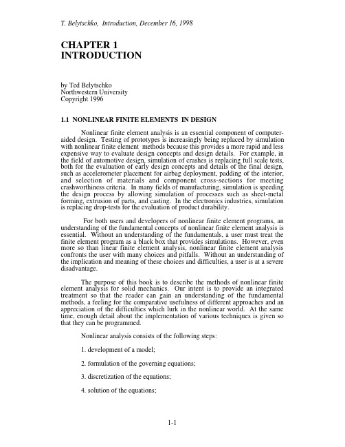
CHAPTER 1INTRODUCTIONby Ted BelytschkoNorthwestern UniversityCopyright 19961.1 NONLINEAR FINITE ELEMENTS IN DESIGNNonlinear finite element analysis is an essential component of computer-aided design. Testing of prototypes is increasingly being replaced by simulation with nonlinear finite element methods because this provides a more rapid and less expensive way to evaluate design concepts and design details. For example, in the field of automotive design, simulation of crashes is replacing full scale tests, both for the evaluation of early design concepts and details of the final design, such as accelerometer placement for airbag deployment, padding of the interior, and selection of materials and component cross-sections for meeting crashworthiness criteria. In many fields of manufacturing, simulation is speeding the design process by allowing simulation of processes such as sheet-metal forming, extrusion of parts, and casting. In the electronics industries, simulation is replacing drop-tests for the evaluation of product durability.For both users and developers of nonlinear finite element programs, an understanding of the fundamental concepts of nonlinear finite element analysis is essential. Without an understanding of the fundamentals, a user must treat the finite element program as a black box that provides simulations. However, even more so than linear finite element analysis, nonlinear finite element analysis confronts the user with many choices and pitfalls. Without an understanding of the implication and meaning of these choices and difficulties, a user is at a severe disadvantage.The purpose of this book is to describe the methods of nonlinear finite element analysis for solid mechanics. Our intent is to provide an integrated treatment so that the reader can gain an understanding of the fundamental methods, a feeling for the comparative usefulness of different approaches and an appreciation of the difficulties which lurk in the nonlinear world. At the same time, enough detail about the implementation of various techniques is given so that they can be programmed.Nonlinear analysis consists of the following steps:1. development of a model;2. formulation of the governing equations;3. discretization of the equations;4. solution of the equations;5. interpretation of the results.Modeling is a term that tends to be used for two distinct tasks in engineering. The older definition emphasizes the extraction of the essential elements of mechanical behavior. The objective in this approach is to identify the simplest model which can replicate the behavior of interest. In this approach, model development is the process of identifying the ingredients of the model which can provide the qualitative and quantitative predictions.A second approach to modeling, which is becoming more common in industry, is to develop a detailed, single model of a design and to use it to examine all of the engineering criteria which are of interest. The impetus for this approach to modeling is that it costs far more to make a model or mesh for an engineering product than can be saved through reduction of the model by specializing it for each application. For example, the same finite element model of a laptop computer can be used for a drop-test simulation, a linear static analysis and a thermal analysis. By using the same model for all of these analyses, a significant amount of engineering time can be saved. While this approach is not recommended in all situations, it is becoming commonplace in industry. In the near future the finite element model may serve as a prototype that can be used for checking many aspects of a design’s performance. The decreasing cost of computer time and the increasing speed of computers make this approach highly cost-effective. However the user of finite element software must still able to evaluate the suitability of a model for a particular analysis and understand its limitations.The formulation of the governing equations and their discretization is largely in the hands of the software developers today. However, a user who does not understand the fundamentals of the software faces many perils, for some approaches and software may be unsuitable. Furthermore, to convert experimental data to input, the user must be aware of the stress and strain measures used in the program and by the experimentalist who provided material data. The user must understand the sensitivity of response to the data and how to asses it. An effective user must be aware of the likely sources of error, how to check for these errors and estimate their magnitudes, and the limitations and strengths of various algorithms.The solution of the discrete equations also presents a user with many choices. An inappropriate choice will result in very long run-times which can prevent him from obtaining the results within the time schedule. An understanding of the advantages and disadvantages and the approximate computer time required for various solution procedures are invaluable in the selection of a good strategy for developing a reasonable model and selecting the solution procedure.The user’s role is most crucial in the interpretation of results. In addition to the approximations inherent even in linear finite element models, nonlinear analyses are often sensitive to many factors that can make a single simulation quite misleading. Nonlinear solids can undergo instabilities, their response can be sensitive to imperfections, and the results can depend dramatically on material parameters. Unless the user is aware of these phenomena, the possibility of a misinterpretation of simulation results is quite possible.In spite of these many pitfalls, our views on the usefulness and potential of nonlinear finite element analyses are very sanguine. In many industries, nonlinear finite element analysis have shortened design cycles and dramatically reduced the need for prototype tests. Simulations, because of the wide variety of output they produce and the ease of doing what-ifs, can lead to tremendous improvements of the engineer's understanding of the basic physics of a product's behavior under various environments. While tests give the gross but important result of whether the product withstands a certain environment, they usually provide little of the detail of the behavior of the product on which a redesign can be based if the product does not meet a test. Computer simulations, on the other hand, give detailed histories of stress and strain and other state variables, which in the hands of a good engineer give valuable insight into how to redesign the product .Like many finite element books, this book presents a large variety of methods and recipes for the solution of engineering and scientific problems by the finite element method. However, in order to preserve a pedagogic character, we have interwoven several themes into the book which we feel are of central importance in nonlinear analysis. These include the following:1. the selection of appropriate methods for the problem at hand;2. the selection of a suitable mesh description and kinematic and kinetic descriptions for a given problem;3. the examination of stability of the solution and the solution procedure;4. an awareness of the smoothness of the response of the model and its implication on the quality and cost of the solution;5. the role of major assumptions and the likely sources of error.The selection of an appropriate mesh description, i.e. whether a Lagrangian, Eulerian or arbitrary Lagrangian Eulerian mesh is used, is very important for many of the large deformation problems encountered in process simulation and failure analysis. The effects of mesh distortion need to be understood, and the advantages of different types of mesh descriptions should be borne in mind in the selection. There are many situations where a continuous remeshing or arbitrary Lagrangian Eulerian description is most suitable.The issue of the stability of solution is central in the simulation of nonlinear processes. In numerical simulation, it is possible to obtain solutions which are not physically stable and therefore quite meaningless. Many solutions are sensitive to imperfections or material and load parameters; in some cases, there is even sensitivity to the mesh employed in the solution. A knowledgeable user of nonlinear finite element software must be aware of these characteristics and the associated pitfalls. Otherwise the results obtained by elaborate computer simulations can be quite misleading and lead to incorrect design decisions.The issue of smoothness is also ubiquitous in nonlinear finite element analysis. Lack of smoothness degrades the robustness of most algorithms and can introduce undesirable noise into the solution. Techniques have been developed which improve the smoothness of the response; these are generally called regularization procedures. However, regularization procedures are often notbased on physical phenomena and in many cases the constants associated with the regularization are difficult to determine. Therefore, an analyst is often confronted with the dilemma of whether to choose a method which leads to smoother solutions or to deal with a discontinuous response. An understanding of the effects of regularization parameters, the presence of hidden regularizations, such as penalty methods in contact-impact, and an appreciation of the benefits of these methods is highly desirable.The accuracy and stability of solutions is a difficult consideration in nonlinear analysis. These issues manifest themselves in many ways. For example, in the selection of an element, the analyst must be aware of stability and locking characteristics of various elements. A judicious selection of an element for a problem involves factors such as the stability of the element for the problem at hand, the expected smoothness of the solution and the magnitude of deformations expected. In addition, the analyst must be aware of the complexity of nonlinear solutions: the appearance of bifurcation points and limit points, the stability and instability of equilibrium branches. The possibility of both physical and numerical instabilities must be kept in mind and checked in a solution.Thus the informed use of nonlinear software in both industry and research requires considerable understanding of nonlinear finite element methods. It is the objective of this book to provide this understanding and to make the reader aware of the many interesting challenges and opportunities in nonlinear finite element analysis.1.2. RELATED BOOKS AND HISTORY OF NONLINEAR FINITE ELEMENTSSeveral excellent texts and monographs devoted either entirely or partially to nonlinear finite element analysis have already been published. Books dealing only with nonlinear finite element analysis include Oden(1972), Crisfield(1991), Kleiber(1989), and Zhong(1993). Oden’s work is particularly noteworthy since it pioneered the field of nonlinear finite element analysis of solids and structures. Some of the books which are partially devoted to nonlinear analysis are Belytschko and Hughes(1983), Zienkiewicz and Taylor(1991), Bathe(1995) and Cook, Plesha and Malkus(1989). These books provide useful introductions to nonlinear finite element analysis. As a companion book, a treatment of linear finite element analysis is also useful. The most comprehensive are Hughes (1987) and Zienkiewicz and Taylor(1991).Nonlinear finite element methods have many roots. Not long after the linear finite element method appeared through the work of the Boeing group and the famous paper of Cough, Topp, and Martin (??), engineers in several venues began extensions of the method to nonlinear, small displacement static problems, Incidentally, it is hard to convey the excitement of the finite element community and the disdain of classical researchers for the method. For example, for many years the Journal of Applied Mechanics banned papers, either tacitly, because it was considered of no scientific substance [sentence does not finish]. The excitement in the method was fueled by Ed Wilson's liberal distribution of his first programs. In many laboratories throughout the world, engineers developed new applications by modifying and extending these early codes.This account form those in many other books in that the focus is not on the published works, buut on the software. In nonlinear finite element analysis, as in many endeavors in this information-computer age, te software represents a more meaningful indication of the state-of-the-art than the literature since it represents what can be applied in practice.Among the first papers on nonlinear finite element methods were Marcal and King (??) and Gallagher (??). Pedro Marcal taught at Brown in those early years of nonlinear FEM, but he soon set up a firm to market the first nonlinear finite element program in 196?; the program was called MARC and is still a major player in the commercial software scene.At about the same time, John Swanson (??) was developing a nonlinear finite element program at Westinghouse for nuclear applications. He left Westinghouse in 19?? to market the program ANSYS, which for the period 1980-90 dominated the commercial nonlinear finite element scene.Two other major players in the early commercial nonlinear finite element scene were David Hibbitt and Klaus-Jürgen Bathe. David worked with Pedro Marcal until 1972, and then co-founded HKS, which markets ABAQUS. Jürgen launched his program, ADINA, shortly after obtaining his Ph.D. at Berkeley under the tutelage of Ed Wilson while teaching at MIT.All of these programs through the early 1990's focused on static solutions and dynamic solutions by implicit methods. There were terrific advances in these methods in the 1970's, generated mainly by the Berkeley researchers and those with Berkeley roots: Thomas J.R. Hughes, Michael Ortiz, Juan Simo, and Robert Taylor (in order of age), were the most fertile contributors, but there are many other who are referenced throughout this book.Explicit finite element methods probably have many different origins, depending on your viewpoint. Most of us were strongly influenced by the work in the DOE laboratories, such as the work of Wilkins (??) at Lawrence Livermore and Harlow (??) at Los Alamos.In ???, Costantino (??) developed what was probably the first explicit finite element program. It was limit to linear materials and small deformations, and computed the internal nodal forces by multiplying a banded form of K by the nodal displacements. It was used primarily on IBM 7040 series computers, which cost millions of dollars and had a speed of far less than 1 megaflop and 32,000 words of RAM. The stiffness matrix was stored on a tape and the progress of a calculation could be gauged by watching the tape drive; after every step, the tape drive would reverse to permit a read of the stiffness matrix.In 1969, in order to sell a proposal to the Air Force, we conceived what has come to be known as the element-by-element technique: the computation of the nodal forces without use of a stiffness matrix. The resulting program, SAMSON, was a two-dimensional finite element program which was used for a decade by weapons laboratories in the U.S. In 1972, the program was extended to fully nonlinear three-dimensional transient analysis of structures and was called WRECKER. This funding program was provided by the U.S. Department of Transportation by a visionary program manager, Lee Ovenshire, who dreamt in the early 1970's that crash testing of automobiles could be replaced by simulation. However, it was not to be, for at that time a simulation of a 300-element nodalover ?? msec of simulation time took 30 hours of computer time, which cost the equivalent of three years of salary of an Assistant Professor ($35,000). The program funded several other pioneering efforts, Hughes' work on contact-impact (??) and Ted Shugar and Carly Ward's work on the modeling of the head at Port Hueneme. But the DOT decided around 1975 that simulation was too expensive (such is the vision of some bureaucrats) and shifted all funds to testing, bringing this far flung research effort to a screeching halt. WRECKER remained barely alive for the next decade at Ford.Parallel work proceeded at the DOE national laboratories. In 1975, Sam Key completed PRONTO, which also featured the element-by-element explicit method. However, his program suffered from the restrictive dissemination policies of Sandia.The key work in the promulgation of explicit finite element codes was John Hallquist's work at Lawrence Livermore Laboratories. John drew on the work which preceded his with discernment, he interacted closely with many Berkeley researchers such as Bob Taylor, Tom Hughes, and Juan Simo. Some of the key elements of his success were the development of contact-impact interfaces with Dave Benson, his awesome programming productivity and the wide dissemination of the resulting codes, DYNA-2D and DYNA-3D. In contrast to Sandia, LLN seemed to place no impediments on the distribution of the program and it was soon to be found in many government and academic laboratories and in industry throughout the world.Key factors in the success of the DYNA codes was the use of one-point quadrature elements and the degree of vectorization which was achieved by john Hallquist. The latter issue has become somewhat irrelevant with the new generation of computers, but this combination enabled the simulation with models of suffiecient sizeto make full-scale simulation of problems such as car crash meaningful. The one-point quadrature elements with consistent hourglass control discussed in Chapter 8 increased the speed of three-dimensional analysis by almost an order of magnitude over fully integrated three-dimensional elements. 1.3 NOTATIONNonlinear finite element analysis represents a nexus of three fields: (1) linear finite element methods, which evolved out of matrix methods of structural analysis; (2) nonlinear continuum mechanics; and (3) mathematics, including numerical analysis, linear algebra and functional analysis, Hughes(1996). In each of these fields a standard notation has evolved. Unfortunately, the notations are quite different, and at times contradictory or overlapping. We have tried to keep the variety of notation to a minimum and both consistent within the book and with the relevant literature. To make a reasonable presentation possible, both the notation of the finite element literature and continuum mechanics are used.Three types of notation are used: 1. indicial notation, 2. tensor notation and 3. matrix notation. Equations in continuum mechanics are written in tensor and indicial notation. The equations pertaining to the finite element implementation are given in indicial or matrix notation.Indicial Notation. In indicial notation, the components of tensors or matrices are explicitly specified. Thus a vector, which is a first order tensor, is denoted inindicial notation by x i , where the range of the index is the number of dimensions n S . Indices repeated twice in a term are summed , in conformance with the rules of Einstein notation. For example in three dimensions, if x i is the position vector with magnitude rr x x x x x x x x x y z i i 2112233222==++=++(1.3.1)where the second equation indicates that x 1=x ,x 2=y ,x 3=z ; we will always write out the coordinates as x, y and z rather than using subscripts to avoid confusion with nodal values. For a vector such as the velocity v i in three dimensions, v 1=v x ,v 2=v y ,v 3=v z ; numerical subscripts are avoided in writing out expressions to avoid confusing components with node numbers. Indices which refer to components of tensors are always lower case .Nodal indices are always indicated by upper case Latin letters, e.g. v iI is the velocity at node I . Upper case indices repeated twice are summed over their range , which depends on the context. When dealing with an element, the range is over the nodes of the element, whereas when dealing with a mesh, the range is over the nodes of the mesh. Thus the velocity at a node I is written as v iI , where v iI is the i-component at node I .A second order tensor is indicated by two subscripts. For example, for thesecond order tensor E ij , the components are E E E E xx yx 1121==,, etc.. We will usually use indicial notation for Cartesian components but in a few of the more advanced sections we also use curvilinear components.Indicial notation at times leads to spaghetti-like equations, and the resulting equations are often only applicable to Cartesian coordinates. For those who dislike indicial notation, it should be pointed out that it is almost unavoidable in the implementation of finite element methods, for in programming the finite element equations the indices must be specified.Tensor Notation. Tensor notation is frequently used in continuum mechanics because tensor expression are independent of the coordinate systems. Thus while Cartesian indicial equations only apply to Cartesian coordinates, expressions in tensor notation can be converted to other coordinates such as cylindrical coordinates, curvilinear coordinates, etc. Furthermore, equations in tensor notation are much easier to memorize. A large part of the continuum mechanics and finite element literature employs tensor notation, so a serious student should become familiar with it.In tensor notation, we indicate tensors of order one or greater in boldface.Lower case bold-face letters are almost always used for first order tensors, while upper case, bold-face letters are used for higher order tensors. For example, a velocity vector is indicated by v in tensor notation, while the second order tensor,such as E , is written in upper case. The major exception to this are the physical stress tensor s , which is a second order tensor, but is denoted by a lower case symbol. Equation(1.3.1) is written in tensor notation asr 2=⋅x x (1.3.2)where a dot denotes a contraction of the inner indices; in this case, the tensors on the RHS have only one index so the contraction applies to those indices.Tensor expressions are distinguished from matrix expressions by using dots and colons between terms, as in a b ⋅, and A B ⋅. The symbol ":" denotes the contraction of a pair of repeated indices which appear in the same order, soA :B ≡A B ij ij (1.3.3)The symbol "⋅⋅" denotes the contraction of the outer repeated indices and the inner repeated indices, as inA B A :B ⋅⋅==A B ij ji T (1.3.4)If one of the tensors is symmetric, the expressions in Eqs. (1.3.3) and (1.3.4) are equivalent. This notation can also be used for contraction of higher order matrices. For example, the usual expression for a constitutive equation given below on the left is written in tensor notation as shown on the rightσεij ijkl kl C = σε=C:(1.3.5)The functional dependence of a variable will be indicated at the beginning of a development in the standard manner by listing the independent variables. For example, v x (,)t indicates that the velocity v is a function of the space coordinates x and the time t . In subsequent appearances of v , the identity of the independent variables in implied. We will not hang symbols all around the variable. This notation, which has evolved in a some of the finite element literature, violates esthetics, and is reminiscent of laundry hanging from the balconies of tenements. We will attach short words to some of the symbols. This is intended to help a reader who delves into the middle of the book. It is not intended that such complex symbols be used working through equations.Mathematical symbols and equations should be kept as simple as possible.Matrix Notation. In implementation of finite element methods, we will often use matrix notation. We will use the same notations for matrices as for tensors and but will not use connective symbols. Thus Eq. (2) in matrix notation is written asr T 2=x x (1.3.6) All first order matrices will be denoted by lower case boldface letters, such as v ,and will be considered column matrices. Examples of column matrices arex =x y z v =v 1v 2v 3(1.3.7)Usually rectangular matrices, of which second tensors are a special case, will be denoted by upper case boldface, such as A. The transpose of a matrix is denoted by a superscript “T” , and the first index always refers to a row number, the second to a column number. Thus a 2x2 matrix A and a 2x3 matrix B are written out as (the order of a matrix is also written with number of rows by number of columns, with rows always first):A =A 11A 12A 21A 22B =B 11B 12B 21B 22 B 13B 23 (1.3.8)In summary, we show the quadratic form associated with A in three notationsx Ax x A x T =⋅⋅=x A x i ij j (1.3.9)The above are all equivalent: the first is matrix notation, the second in tensor notation, the third in indicial notation.Second-order tensors are often converted to Voigt. Voigt notation is described in the Glossary.1.4. MESH DESCRIPTIONSOne of the themes of this book is partially the different descriptions that are used in the formulation of the governing equations and the discretization of the continuum mechanics. We will classify the finite element model in three parts, Belytschko (1977):1. the mesh description;2. the kinetic description, which is determined by the choice of the stress tensor and the form of the momentum equation;3. the kinematic description, which is determined by the choice of the strain measure.In this Section, we will introduce the types of mesh descriptions. For this purpose, it is useful to introduce some definitions and concepts which will be used throughout this book. The first are the definitions of material coordinates and spatial coordinates. Spatial coordinates are denoted by x ; spatial coordinates are also called Eulerian coordinates. A spatial (or Eulerian coordinate) specifies the location of a point in space. The material coordinates, also called Lagrangian coordinates, are denoted by X . The material coordinate labels a material point:each material point has a unique material coordinate, which is usually taken to be its spatial coordinate in the initial configuration of the body, so at t=0, X =x .Since in a deforming body, the positions of the material points change with time,the spatial coordinates of material points will be functions of time.The motion or deformation of a body can be described by a functionφX ,t (), with the material coordinates X and the time t as the independentvariables. This function gives the spatial positions of the material points as a function of time through:x X =()φ,t (1.4.1)This is also called a map between the initial and current configurations. The displacement of a material point is the difference between its current position and its original position, so it is given byu X (,),X t X t =()−φ(1.4.2)To illustrate these definitions, consider the following motion in one dimension: x X t X t Xt X ==−++φ(,)()1122(1.4.3)This motion is shown in Fig. 1.1; the motion of several points are plotted in space time to exhibit their trajectories; we obviously cannot plot the motion of all material points since there are an infinite number. The velocity of a material point is the time derivative of the motion with the material coordinate fixed, i.e. the velocity is given byv X t X t t X t (,)(,)==+−()∂φ∂11(1.4.4)The mesh description is based on the choice of independent variables. For purposes of illustration, let us consider the velocity field. We can describe the velocity field as a function of the Lagrangian (material) coordinates, as in Eq.(1.4.4) or we can describe the velocity as a function of the Eulerian (spatial)coordinates v x v x (,),,t t t =()()−φ1(1.4.5)In the above we have placed a bar over the velocity symbol to indicate that the velocity field when expressed in terms of the spatial coordinate x and the time t will not be the same function as that given in Eq. (1.4.4), although in the remainder of the book we will usually not distinguish different functions which are used to represent the same field. We have also used the concept of an inverse map which to express the material coordinates in terms of the spatial coordinatesX x t =()−ϕ1, (1.4.6)Such inverse mappings can generally not be expressed in closed form for arbitrary motions, but for the simple motion given in Eq. (1.4.3) it is given byX x tt t =−−+1221(1.4.7)Substituting the above into (3) gives。
a first course in the finite element method pdf
A First Course in the Finite Element MethodPDF引言:"A First Course in the Finite Element Method" 是一本深受工程学和计算力学领域学生与专业人士推崇的教材。
本文将深入探讨这本书的重要性、内容特点以及它在学术和实际应用中的价值。
1. 书籍概述:"A First Course in the Finite Element Method" 是一本由Daryl L. Logan编写的教材,专注于有限元方法的初学者。
该书旨在为读者提供对这一数值分析技术的全面了解,从基本概念到实际应用。
2. 有限元方法的基础:这本书首先介绍了有限元方法的基础知识,包括数学背景、结构分析和材料力学等基本概念。
通过清晰的解释和实例,读者能够建立对有限元分析的坚实理论基础。
3. 实用的例子和案例:为了使理论更具实际应用性,该教材提供了丰富的实例和案例。
这些例子涵盖了结构工程、热力学、流体力学等多个领域,使学习者能够将所学知识灵活应用于不同领域的工程问题。
4. 计算工具的使用:一项成功的有限元分析离不开有效的计算工具。
本书引导读者使用一些常见的有限元软件,如ANSYS和ABAQUS。
这种实际操作的引导有助于读者更好地理解理论知识,并能够在实际工程问题中应用所学技术。
5. 适用于学术和职业发展:"A First Course in the Finite Element Method" 既适用于大学本科和研究生课程,也是从业工程师的理想参考资料。
它为学术界和工程实践提供了一种通用的学习路径,使学生和专业人士能够在有限元分析领域取得成功。
6. 理论与实践的平衡:一些有关数值分析的教材可能过于理论化,而忽略了实际问题的应用。
这本书通过理论与实践的平衡,使读者在掌握有限元方法的同时,能够解决实际工程中的挑战。
有限元分析作业报告英文版1
有限元分析与应用上机实验报告学院:机电工程学院专业:机械工程班级:硕士1606班*名:***学号: *********指导教师:***日期: 2016.12.021.QuestionFig.1. Schematic diagram of herringbone roof truss.Question: The geometric dimensions of the chevron roof is shown in Fig.1,you should analyze it by statics,as a result you should give the displacement and axial force and axial force diagram of the deformation diagram.Conditions: The ends of the roof truss were fixed, the sectional area of the truss is 0.01m2, elastic modulus is2.0×1011 N/m2, poisson's ratio is 0.3.2.The software usedANSYS Finite element software (APDL 15.0)3.Solving processPoint 1 was choosed as the Coordinate point, horizontal to the right was the X axis,the upright direction is choosed as the Y axis to create a coordinate system. The nodes was numbered as shown in Figure 1,node 1 and node 5 was fixed,and the force on node 6,7,8 was is 1k N,the direction is opposite to the Y-axis3.1 The preparatory work before analysis(1)Specify the new file name. Select Utility>Menu> File>Change Jobname, then pop-up the dialog box Change Jobname, input the the working file name ‘2D-sp’ in the Enter New Jobname, click OK to finish the difinition, as shown in Fig.2.Fig.2. The difinition of working file name.(2)Specify a new title. Select Utility>Menu>File>Change Title,then pop-up the dialog box Change Title, input the the file name ‘2D-sp pro’ in the Enter New Title, click OK to finish the difinition, as shown in Fig.3.Fig.3. The difinition of file name.(3)Re-refresh the graphics window.Select Utility>Menu>Plot>Replot, the defined information was displayed in the graphics window.(4)Define the structural analysis. Run the main menu Main Menu>Preferences,then choose the Structural, click OK to complete the definition of the analysis type , as shown in Fig.4.Fig.4. The definition of the structural analysis.3.2 Define the element typeRun the main menu Main Menu>Preprocessor>Element Type>Add, then pop-up the dialog box Element Types, click the button Add to build a new element type, then pop-up the dialog box Library of Element Types, choose Link first, and then select 3D finit stn 180(Link1),click the button OK to finish the definition of the element type, click the button Close to finish the settings, as shown in Fig.5.Fig.5. The definition of the element type.3.3 Define the real constantsRun the main menu Main Menu>Preprocessor>Real Constants Add, then pop-up the dialog box of real constants, click the button Add to come into the constant input dialog box, as shown in Fig.6. Input the sectional area of the truss (0.01m2) in AREA, click the button OK to finish the input of the real constants, as shown in Fig.7.Fig.6. Get into the instance constant dialog box.Fig.7. The definition of the real constants.3.4 Define the material propertiesRun the main menu Main Menu>Preprocessor>Material Props>Material Models,then pop-up the dialog box of material properties, and select Structure、Linear、Elastic、Isotropic, as shown in Fig.8.When the selection was completed, appeared the MaterialProperties input dialog box appears,then input elastic modulus 2e11 and the poisson's ratio 0.3, as shown in Fig.9, click OK to finish the input of the material properties.Fig.8. Get into the setting of material properties.Fig.9. The difinition of the material properties.3.5 Establish the analytical model(1)Create the nodes. The coordinates of the 1—8 nodes as shown in Table.1. Run the main menu Main Menu>Preprocessor> Modeling>Create>Nodes>In Active CS. The create node entry dialog box appears as shown in Fig.10. I nput the first node 1 and its’ x, y, z coordinate, then click Apply to finish the creating of the node. Similarly, create the nodes 2—8, click OK to finish the creating of the nodes, as shown in Fig.10.Table.1.The coordinates of geometry model nodes.Fig.10. The dialog box of nodes input.Fig.11. The creation of the nodes.The created nodes as shown below:(2)Created the bar unitRun the main menu MainMenu>Preprocessor>Modeling>Create >Elements>Auto Numbered>Thru Nodes, then pop-up the dialog box Element from Nodes, pick the nodes 1 and 2, click Apply to complete the first lever unit . Similarly, pick both ends of the rod in turn, click Apply to complete the lever unit, lastly click OK, as shown in Fig.12.Fig.12. Model establishment of the herringbone truss.3.6 Apply constraints and loads(1)Impose constraintsRun the main menu Main Menu>Solution>Define Loads>Apply>Structural> Displacement>On Nodes, the pick menu appears, select nodes 1 and 5 in turn, then click OK, the constraint definition dialog box appears,as shown in Fig.13. Choose All DOF to constrain all degrees of freedom,other items by default,then click the button OK to complete the constraint definition.Fig.13. Impose the constraints.(2)Apply the loadRun the main menu Main Menu>Solution>Define Loads>Apply>Structural> Force/Moment>On Nodes, the pick menu appears, select nodes 6, 7 and 8 in turn, click OK , then the load definitions dialog box appears,as shown in Fig.14. The load type is concentrated force FY. The value is -1000 , Then clickthe OK button to complete the application of the load.Fig.14. The application of the load.Figure after load application as shown below:3.7 SolutionRun the main menu Main Menu>Solution>Solve>Current LS, then pop-up the dialog box Solve Current Load Step, click STAT Command, then click STAT Command>File>Close toclose the STAT Command window, then click OK to finish the steps.Then the computer started the solution. The promption of "Solution is done" indicated that the solution was completed, click the button Close to finish the solution, as shown in Fig.15.Fig.15. The process of the solution.3.8 View the analysis results(1)Define the cell table. In ANSYS, some data can not be directly accessed, so we need to complete the definition of cell to access the results.Run the main menu Main Menu>General Postproc>Element Table>Define Table, then pop-up the dialog box, click the button Add. The unit table definition dialog box appeared, as shown in Fig.16.Fig.16a. The definition of the cell table.Fig.16b. The definition of the cell table.(2)Display the axial force (axial stress) diagram. Run the main menu Main Menu>General Postproc>Plot Results> Contour Plot>Elem Table. Then pop-up the cell table result selection dialog box , as shown in Fig.17. Choose A-STR and click OK to view the axial force (axial stress) diagram , as shown in Fig.18.Fig.17. Contor plot of Element Table Data.(3)Display the result. The result as shown in Fig.18.Fig.18. The final result.。
有限元英语文献及译文

7. INTRODUCTION TO THE FINITE ELEMENT METHODEngineers use a wide range of tools and techniques to ensure that the designs they create are safe. However, accidents sometimes happen and when they do, companies need to know if a product failed because the design was inadequate or if there is another cause, such as an user error. But they have to ensure that the product works well under a wide range of conditions, and try to avoid to the maximum a failure produced by any cause. One important tool to achieve this is the finite element method.“The finite element method is one of the most powerful numerical techniques ever devised for solving differential (and integral) equations of initial and boundary-value problems in geometrically complicated regions.” (Red dy, 1988). There is some data that can not be ignored when analyzing an element by the finite element method. This input data is to define the domain, the boundary and initial conditions and also the physical properties. After knowing this data, if the analysis is done carefully, it will give satisfactory results. It can be said that the process to do this analysis is very methodical, and that it is why it is so popular, because that makes it easier to apply. “The finite element analysis of a problem is so systematic that it can be divided into a set of logical steps that can be implemented on a digital computer and can be utilized to solve a wide range of problems by merely changing the data input to the computer program.” (Reddy,1988).The finite element analysis can be done for one, two and three-dimensional problems. But generally, the easier problems are those including one and two dimensions, and those can be solved without the aid of a computer, because even if they give a lot of equations, if they are handled with care, an exact result can be achieved. But if the analysis requires three-dimensional tools, then it would be a lot more complicated, because it will involve a lot of equations that are very difficult to solve without having an error. That is why engineers have developed softwares that can perform these analyses by computer, making everything easier. These softwares can make analysis of one, two and threedimensional problems with a very good accuracy.A basic thing to understand how finite element works is to know that it divides the whole element into a finite number of small elements. “The domain of the problem is viewed as a collection of nonintersecting simple subdomains, called finite elements… The subdivision of a domain into elements is termed finite element discretization. The collection of the elements is called the finite element mesh of the domain.” (Reddy,1988). The advantage of dividing a big element into small ones is that it allows that every small element has a simpler shape, which leads to a good approximation for the analysis. Another advantage is that at every node (the intersection of the boundaries) arises an interpolant polynomial, which allows an accurate result at a specific point. Before the finite element method, engineers and physicians used a method that involved the use of differential equations, which is known as the finite difference method.The method of the finite element is a numerical technique that solves or at least approximates enough to a solution of a system of differential equations related with a physics or engineering problem. As explained before, this method requires a completely defined geometrical space, and then it would be subdivided into small portions, which together will form a mesh. The difference between the method of the finite element and the method of the finite difference is that in the second one, the mesh consists of lines and rows of orthogonal lines, while in the method of the finite element the division does not necessarily involves orthogonal lines, and this results in a more accurate analysis (Figure 38).Figure 38 (taken from Algor 13 ®)The equations used for the finite element method are a lot, but they have the basison some single equations that describe a particular phenomenon. Those equations are:The elliptic equation is described by22220 dx dy∂Φ∂Φ+=The parabolic equation is described by220 dx t∂Φ∂Φ-=∂The hyperbolic equation is described by221 220 t x∂Φ∂Φ-=∂∂No matter which is the cause of the internal forces and the deformation that they cause, there are three basic conditions that allow the finite element analysis: the equilibrium of forces, the compatibility of displacements and the laws of material behavior. “The first condition merely requires that the internal forces balance the external applied loads.” (Rocke t et. al., 1983). That is the most important condition, but the other two assure that the system will be a statically determinate problem. Another condition that must be taken into account is that there exists a relationship between the load applied and the deformation, and this is given by Hooke’s law, as explained in past chapters, but only in the elastic range.In order to achieve a structural analysis by matrix methods, there might be threeways: stiffness (displacement) method, flexibility (force) method and mixed method. In the first two methods, two basic conditions of nodal equilibrium and compatibility must be reached. In the first method, the once the displacement compatibility conditions are reached, then an answer can be given. In the second method, once the conditions of nodal equilibrium are satisfied and then the compatibility of nodal displacement, forces are known in the members.One of the principles that is the basis of the finite element method is the one known as principle of virtual work. “This principle is conc erned with the relationship which exists between a set of external loads and the corresponding internal forces which together satisfy the equilibrium condition, and also with sets of joint (node) displacements and the corresponding member deformations which satisfy the conditions of compatibility.” This principle can be stated in terms of an equation of equilibrium of loads, where the work done by the external loads is equal to the internal virtual work absorbed by the element. Or expressed as an equation:v F d δσε⋅ =⋅⋅∑⎰where F are the external loads, the deflection, the system of internal forces, and the internal deformations.A pin ended tie has similar characteristics to those of an elastic spring that is subjected on one end, looking downwards, suffering the effects of gravity and the effect of an external load. The direct relationship between the force and the displacement of the free end is:F k δ=⋅the vale k is known as the stiffness of the spring. Once the value of the applied force and the value of the stiffness, the equation can be inverted to find the displacement: 1F kδ= This is a simple example for systems that imply only a few data. But when the problem implies more complex systems, then the equations become a little more complicated. When a number of simple members are interconnected at a number of nodes, the displacement caused by the load can only be described by simultaneous equations. Then, the simpler equation seen before becomes:{}[]{}F K δ=where K is the stiffness of the whole structure.For example, for a spring that has two pins, it generates two forces and two displacements. Therefore, the stiffness matrix would be of order 2 x 2:111121221222F k k u F k k u ⎧⎫⎡⎤⎧⎫=⎨⎬⎨⎬⎢⎥⎩⎭⎣⎦⎩⎭where u represents the displacement.Boundary conditions are the limitations set for the problem. These limitations are necessary in order to solve it, because otherwise, the system would be taken as a rigid body. The limitations stated by these boundary conditions are like where does the element is likely to move, and were it is restricted. If there were not boundary conditions, the body would be floating in the space, and under the action of any load, it would not suffer any deformation, but it would move around the space as a rigid body. So, when assuming boundary conditions, it has to be assured that the element has enough of them in order to prevent moving as a rigid body. Once this is done, the values of the displacements are obtained and can be substituted in the last equation seen, which will give that the displacement is equal to zero, because the element can not move in any direction. Then, algebra is applied, and the values of the forces or of the stiffness are known.7.1 Applications of the finite element method in engineeringEvery designed made has to fulfill certain specifications, and among them is working under a variety of conditions: temperature, humidity, vibrations, etc. The job of the designer is to achieve this, and to assure that the product will work effectively, taking care of the user and of the element. An engineer has to follow certain steps in order to create a good product with high quality. First, the steps of the design flow chart must be followed:1. recognize a need2. specifications and requirements3. feasibility sturdy4. creative design and development5. detailed drawings6. prototype building and testing7. design for manufactureThese are the basic concepts of the design, but it involves a lot of other things to be able to assure a good performance of the product. After the designer has the calculations of the dimensions, tolerances, manufacturing parameters, etc, some other tests should be done. For example, an engineer has to know whether the product is going to support certain loads, or how it is going to behave with temperature variations, or what could happen if vibrations are present. This is where the finite element method enters in action in engineering.In the last pages, it has been explained how the finite element works and which are the basis of it. Now it is time to explain what is it good for, the applications, the benefits, etc. For example, the first application of the method was introduced by Richard Courant to solve torsion on a cylinder. Then, in the middle 50’s, the method started to be applied for airframe and structural analysis, and then used in civil engineering. In general, finite element methods are used in a wide variety of engineering applications, like in computer graphics, heat transfer, electrical and magnetic fields, among others.Use of finite element method in mechanical engineering is very wide. For example, it is used in mechanics of materials, for structures and trusses. It is used to understand and to prevent how some structures are going to behave under the action of some loads. For example, for a bridge, how is it going to behave with the vibrations, or with the effect of the air, or with the variations of temperature. The aircraft industry uses this method to determine the static and dynamic answer of planes and space crafts to the great variety of environments and conditions that can be found during their operation.In the case of mechanics of fluids, the method is used to know how a wing of a plane is going to behave with the air flux passing through it, if it is going to resist, how much vibration is this going to cause, in order to avoid resonance (because of the vibrations caused by the turbines too). The finite element method allows calculating the drag and the flotation forces caused during operation.For heat transfer, it allows to know how a turbine is going to behave, and how the material is going to be affected for the effect of the heat. It is known that heat also creates stresses, and this is a fundamental concept when talking about design of turbines. Another important thing to mention here is that when turbines are working, they reach very high temperatures, and they use a coolant to maintain the temperature under some point. This coolant, when touching the hot turbine, creates a thermal shock, which also producesstresses. These stresses can be measured through the finite element method. Something else that it is important is that some components of the turbine (like blades) have holes to let the air in to act as a coolant to avoid overheating. These holes can act as stress concentrators, and by this method, it can be analyzed which is the way they affect less the stress distribution.One important area where this method is used is in design of mechanical elements. Generally, these elements have to support high loads, whether they are radial, tension, compression, tangential, etc. Sometimes these loads are combined, which makes the element designed more prone to failure. Most of the time, mechanical parts also have holes for assembly, for flow of a certain fluid, etc, and these holes create stress concentrations. A very specific and careful analysis has to be made. Here is where the finite element analysis plays an important role. For example, in the design of a crank, it is subjected to different loads, and it has specific boundary conditions. It is tested with total restriction on one side, and with a load applied tangentially on the other side. The results are like in Figure 39, where the areas that have bigger stresses can be identified according to the color specified on the right of the screen.Figure 39Other application in design is in the design of a control arm. This is for a combination of mechanics with electronics, but it still has forces applied, and holes manufactured for assembly. The boundary conditions have to be established according to the allowable movements of the robot, and then the loads applied in the points where it carries something. The results are those in Figure 40Figure 40The automotive industry uses this method to see how the cars behave under some conditions of load, and for crash tests. For this industry, it has a lot of advantages. After the car is modeled in a CAD software, it is exported to a finite element analysis software, and after all the conditions are set, the test begins. The method has the advantage of giving very accurate information. For example, the deformation suffered point by point (node by node) at a specific time. The fact of they doing these type of analyses represents a great advantage for them, because they save money, they save time, and they also save material, and yet they have very reliable information of the behavior of the car. For example, Figure 41, which is a model of a thesis done the last semester, where the student was analyzing the effect of the impact on the car, and also on a dummy. He could calculate the stress at any point he wanted to, and at any time of the collision, and he was able to determine which areas of the car and the dummy were the most affected with the impact. Another example is Figure 42.Figure 41 (from Alfredo Pérez Mitre)Figure 427.2 AdvantagesThe use of the finite element method has a lot of advantages, and most of them have already been commented in this thesis, but here it is going to be made a short condensation of them.First, it is a very important tool for stress and strain analysis, not only because it provides accurate information, but because it also saves a lot of money and time by simulating the events in computer and not in real life. It is a really easy to use tool. Once some tutorials are followed, the only thing left to do is to explore a little bit of the software, and then to apply all the knowledge acquired. The principles of the method are easy to understand, even if when the model is complex, the analyses are also complex.For every engineer it is a very reliable tool, because it is very specific for each occasion, and it is able to perform different analyses of the same model under different circumstances with simple changes in the boundary conditions, in the loads, in the material, or whatever the problem demands.The method can help to modify each design in order to increase the service life of it as much as possible. That is the case of study of this thesis, where some analyses are run in the computer to see how the presence of a stress concentrator affects the behavior of the element. If the stress concentration is high, the element can be modified with ease and thensubjected to analysis again, and depending on the results, a decision has to be taken to see if it needs more changes or if it has reached or if it is even close to its maximum service life condition.The combination of this as a software with other types of softwares is a very useful tool, because the program of finite element analysis allows the designer to import models from other CAD softwares, and that way it does not forces the engineer to make the solid in the FEA CAD. That way, complex models can be created and analyzed with the combination of those two powerful tools.7.有限元方法的简介工程师需要使用范围更广的工具和技术来保证他们创建的设计是安全的。
《有限元分析》课程全英文授课教学实践

外语·外文 课程教育研究 Course Education Ressearch 2015年1月 下旬刊116· ·务的教师,不仅需要较强的英语听说读写能力,更应该重视教师英语的专业性考察,在这样的基础上,还需要不断地学习,增强自身的实力,学习先进的教学理念,更好地指导学生学习英语。
(三)提高教学方法正如前面所谈到的,对飞机维修说明的理解绝不是一两个常见单词或句型就可以弄清楚的,单词的多重含义,句子的结构,这都影响着英语阅读的正确理解,所以在平时的教学中,教师要有目的地提高学生的阅读分析能力,教导学生阅读的技巧,在第一遍快速阅读的时候了解文章大意,在此基础上,再由教师逐层详细讲解,培养英语阅读思维;同时还要重视文章的朗读,因为里面涉及了很多专业名词和术语,通过这样重复阅读,可以加强学生对它们的理解与背诵。
除此之外,课外阅读也是必不可少的,能够扩大学生的知识面,为提高阅读能力打下基础。
参考文献:[1] 罗海燕,申翰林,周超等.机务人才专业英语水平提升的探索与思考[J].中国民用航空,20113(12):109-110.[2] 慕永锋,张杏辉.民航院校机务类学生素质教育研究[J].时代教育,2014(03):72+78.[3] 王凌燕.浅谈对艺术类英语学困生进行有效教学[J].价值工程,2012(08):209-210.[4] 张驰.航空维修专业英语教学现状分析与解决途径[J].英语广场(学术研究),2012(10):99-101.[5] 张永利,裴育新.艺术类大学生英语学习现状与教学策略探析[J].求实,2014(S1):250-251.本文系2013年湖南省教育科学“十二五”规划一般课题《高职院校航空机务类英语课程教学改革的研究与实践》的部分成果,项目批准号XJK013CZY032”《有限元分析》课程全英文授课教学实践李红军(浙江理工大学机械与自动控制学院 浙江 杭州 310018)【摘要】随着我国高等教育的发展,课程建设的国际化也成为了我国高校教育改革的一个重要课题和发展方向。
机器人机构优化设计有限元分析毕业论文中英文资料对照外文翻译文献综述
机器人机构优化设计有限元分析中英文资料对照外文翻译文献综述FEM Optimization for Robot StructureAbstractIn optimal design for robot structures, design models need to he modified and computed repeatedly. Because modifying usually can not automatically be run, it consumes a lot of time. This paper gives a method that uses APDL language of ANSYS 5.5 software to generate an optimal control program, which mike optimal procedure run automatically and optimal efficiency be improved.1)IntroductionIndustrial robot is a kind of machine, which is controlled by computers. Because efficiency and maneuverability are higher than traditional machines, industrial robot is used extensively in industry. For the sake of efficiency and maneuverability, reducing mass and increasing stiffness is more important than traditional machines, in structure design of industrial robot.A lot of methods are used in optimization design of structure. Finite element method is a much effective method. In general, modeling and modifying are manual, which is feasible when model is simple. When model is complicated, optimization time is longer. In the longer optimization time, calculation time is usually very little, a majority of time is used for modeling and modifying. It is key of improving efficiency of structure optimization how to reduce modeling and modifying time.APDL language is an interactive development tool, which is based on ANSYS and is offered to program users. APDL language has typical function of some large computer languages. For example, parameter definition similar to constant and variable definition, branch and loop control, and macro call similar to function and subroutine call, etc. Besides these, it possesses powerful capability of mathematical calculation. The capability of mathematical calculation includes arithmetic calculation, comparison, rounding, and trigonometric function, exponential function and hyperbola function of standard FORTRAN language, etc. By means of APDL language, the data can be read and then calculated, which is in database of ANSYS program, and running process of ANSYS program can be controlled.Fig. 1 shows the main framework of a parallel robot with three bars. When the length of three bars are changed, conjunct end of three bars can follow a given track, where robot hand is installed. Core of top beam is triangle, owing to three bars used in the design, which is showed in Fig.2. Use of three bars makes top beam nonsymmetrical along the plane that is defined by two columns. According to a qualitative analysis from Fig.1, Stiffness values along z-axis are different at three joint locations on the top beam and stiffness at the location between bar 1 and top beam is lowest, which is confirmed by computing results of finite element, too. According to design goal, stiffness difference at three joint locations must he within a given tolerance. In consistent of stiffness will have influence on the motion accuracy of the manipulator under high load, so it is necessary to find the accurate location of top beam along x-axis.To the questions presented above, the general solution is to change the location of the top beam many times, compare the results and eventually find a proper position, The model will be modified according to the last calculating result each time. It is difficult to avoid mistakes if the iterative process is controlled manually and the iterative time is too long. The outer wall and inner rib shapes of the top beam will be changed after the model is modified. To find the appropriate location of top beam, the model needs to be modified repetitiously.Fig. 1 Solution of Original DesignThis paper gives an optimization solution to the position optimization question of the top beam by APDL language of ANSYS program. After the analysis model first founded, the optimization control program can be formed by means of modeling instruction in the log file. The later iterative optimization process can be finished by the optimization control program and do not need manual control. The time spent in modifying the model can be decreased to the ignorable extent. The efficiency of the optimization process is greatly improved.2)Construction of model for analysisThe structure shown in Fig. 1 consists of three parts: two columns, one beam and three driving bars. The columns and beam are joined by the bolts on the first horizontal rib located on top of the columns as shown in Fig.1. Because the driving bars are substituted by equivalentforces on the joint positions, their structure is ignored in the model.The core of the top beam is three joints and a hole with special purpose, which can not be changed. The other parts of the beam may be changed if needed. For the convenience of modeling, the core of the beam is formed into one component. In the process of optimization, only the core position of beam along x axis is changed, that is to say, shape of beam core is not changed. It should be noticed that, in the rest of beam, only shape is changed but the topology is not changed and which can automatically be performed by the control program.Fig.1, six bolts join the beam and two columns. The joint surface can not bear the pull stress in the non-bolt joint positions, in which it is better to set contact elements. When the model includes contact elements, nonlinear iterative calculation will be needed in the process of solution and the computing time will quickly increase. The trial computing result not including contact element shows that the outside of beam bears pulling stress and the inner of beam bears the press stress. Considering the primary analysis object is the joint position stiffness between the top beam and the three driving bars, contact elements may not used, hut constructs the geometry model of joint surface as Fig.2 showing. The upper surface and the undersurface share one key point in bolt-joint positions and the upper surface and the under surface separately possess own key points in no bolt positions. When meshed, one node will be created at shared key point, where columns and beam are joined, and two nodes will be created at non shared key point, where column and beam are separated. On right surface of left column and left surface of right column, according to trial computing result, the structure bears press stress. Therefore, the columns and beam will share all key points, not but at bolts. This can not only omit contact element but also show the characteristic of bolt joining. The joining between the bottoms of the columns and the base are treated as full constraint. Because the main aim of analysis is the stiffness of the top beam, it can be assumed that the joint positions hear the same as load between beam and the three driving bars. The structure is the thin wall cast and simulated by shell element . The thickness of the outside wall of the structure and the rib are not equal, so two groups of real constant should he set. For the convenience of modeling, the two columns are alsoset into another component. The components can create an assembly. In this way, the joint positions between the beam core and columns could he easily selected, in the modifying the model and modifying process can automatically be performed. Analysis model is showed Fig.1. Because model and load are symmetric, computing model is only half. So the total of elements is decreased to 8927 and the total of nodes is decreased to 4341. All elements are triangle.3.)Optimization solutionThe optimization process is essentially a computing and modifying process. The original design is used as initial condition of the iterative process. The ending condition of the process is that stiffness differences of the joint locations between three driving bars and top beam are less than given tolerance or iterative times exceed expected value. Considering the speciality of the question, it is foreseen that the location is existent where stiffness values are equal. If iterative is not convergent, the cause cannot be otherwise than inappropriate displacement increment or deficient iterative times. In order to make the iterative process convergent quickly and efficiently, this paper uses the bisection searching method changing step length to modify the top beam displacement. This method is a little complex but the requirement on the initial condition is relatively mild.The flow chart of optimization as follows:1. Read the beam model data in initial position from backup file;2. Modify the position of beam;3. Solve;4. Read the deform of nodes where beam and three bars are joined;5. Check whether the convergent conditions are satisfied, if not, then continue to modify the beam displacement and return to 3, otherwise, exit the iteration procedure.6. Save the results and then exit.The program's primary control codes and their function commentaries are given in it, of which the detailed modeling instructions are omitted. For the convenience of comparing with the control flow, the necessary notes are added.the flag of the batch file in ANSYSBATCH RESUME, robbak.db, 0read original data from the backupfile robbak,.db/PREP7 enter preprocessordelete the joint part between beam core and columnsmove the core of the beam by one :step lengthapply load and constraint on the geometry meshing thejoint position between beam core and columns FINISH exit the preprocessorISOLU enter solverSOLVE solveFINISH exit the solverPOST1 enter the postprocessor*GET ,front,NODE,2013,U,Z read the deformation of first joint node on beam*GET,back,NODE, 1441 ,U,Z read the deformation of second joint node on beam intoparameter hacklastdif-1 the absolute of initial difference between front and hacklast timeflag=- 1 the feasibility flag of the optimizationstep=0.05 the initial displacement from initial position to the currentposition*D0,1,1,10,1 the iteration procedure begin, the cycle variable is I andits value range is 1-10 and step length is 1dif=abs(front-back) the absolute of the difference between front and hack inthe current result*IF,dif,LE,l .OE-6,THEN check whether the absolute difference dif satisfies therequest or noflag=l yes, set flag equal to 1*EXIT exit the iterative calculation*ELSEIF,dif,GE,lastdif,THEN check whether the dif value becomes great or not flag=2yes, set flag 2 modify step length by bisection methodperform the next iterative calculation, use the lastposition as the current position and modified last steplength as the current step lengthELSE if the absolute of difference value is not less thanexpected value and become small gradually, continue tomove top beam read the initial condition from back upfile enter the preprocessorMEN, ,P51X, , , step,, , ,1 move the core of the beam by one step length modify thejoint positions between beam core and column applyload and constraint meshingFINISH exit preprocessorISOLU enter solverSOLVE solveFINISH exit the solver/POST1 exit the postprocessor*GET,front,NODE,201 3,U,Z read the deformation of first joint node to parameter front *GET,back,NODE, 144 1,U,Z read the deformation of second joint node to parameter back lastdif-dif update the value of last dif*ENDIF the end of the if-else*ENDDO the end of the DO cycleMost of the control program above is copied from log file, which is long. The total of lines is up to about 1000 lines. Many codes such as modeling and post-process codes are used repeatedly. To make the program construct clear, these instructions can he made into macros, which are called by main program. This can efficiently reduce the length of the main program. In addition, modeling instructions from log file includes lots of special instructions that are only used under graphic mode but useless under hatch mode. Deleting and modifying these instructions when under batch mode in ANSYS can reduce the length of the file, too.In the program above, the deformation at given position is read from node deformation. In meshing, in order to avoid generating had elements, triangle mesh is used. In optimization, the shape of joint position between columns and beam continually is changed. This makes total of elements different after meshing each time and then element numbering different, too. Data read from database according to node numbering might not he data to want. Therefore, beam core first needs to he meshed, then saved. When read next time, its numbering is the same as last time.Evaluating whether the final result is a feasible result or not needs to check the flag value. If only the flag value is I, the result is feasible, otherwise the most proper position is not found. The total displacement of top beam is saved in parameter step. If the result is feasible, the step value is the distance from initial position to the most proper position. The sum of iterative is saved in parameter 1. According to the final value of I, feasibility of analysis result and correctness of initial condition can he evaluated.4)Optimization resultsThe sum of iterative in optimization is seven, and it takes about 2 hour and 37 minutes to find optimal position. Fig.3 shows the deformation contour of the half-construct. In Fig.3, the deformations in three joints between beam and the three driving bars is the same as level, and the corresponding deformation range is between -0.133E-04 and -0.1 15E-O4m, the requirement of the same stiffness is reached. At this time, the position of beam core along x-axis as shown in Fig. 1 has moved -0.71E-01m compared with the original designed positionBecause the speed of computer reading instruction is much faster than modifying model manually, the time modifying model can be ignored. The time necessary foroptimization mostly depends on the time of solution. Compared with the optimization procedure manually modifying model, the efficiency is improved and mistake operating in modeling is avoided.5)ConclusionThe analyzing result reveals that the optimization method given in this paper is effective and reaches the expected goal. The first advantage of this method is that manual mistakes do not easily occur in optimization procedure. Secondly, it is pretty universal and the control codes given in this paper may he transplanted to use in similar structure optimization design without large modification. The disadvantage is that the topology structure of the optimization object can not be changed. The more the workload of modifying the model, the more the advantages of this method are shown. In addition, the topology optimization function provided in ANSYS is usedto solve the optimization problem that needs to change the topology structure.The better optimization results can he achieved if the method in this paper combined with it.中文译文:机器人机构优化设计有限元分析摘要机器人结构最优化设计,设计模型需要反复的修正和计算。
有限元分析ujoint有限元分析论文

有限元分析课程论文课程名称:有限元分析论文题目:ujoint有限元分析学生班级;学生姓名:任课教师:学位类别:评分标准及分值选题与参阅资料(分值)论文内容(分值)论文表述(分值)创新性(分值)评分论文评语:总评分评阅教师: 评阅时间年月日注:此表为每个学生的论文封面,请任课教师填写分项分值基于abaqus的ujoint有限元分析摘要:万向传动装置在汽车中起到了传递扭矩的关键作用,在abaqus中导入ujoint实体模型,之后对其进行坐标系建立,wire 建立,以及各部件之间的连接关系的建立,最后对该模型施加边界条件,令其运动。
关键词:abaqus、有限元、ujoint一问题的描述对导入的ujoint在所有步骤完成后,施加力:在stepinitial:均设为0;step SPIN:doundary1:限制除UR2的所有,且把UR2值设为:pi。
在boundary2 中,限制UR1和UR3自由度。
二在abaqus中导入ujoint实体模型启动abaqus CAE,在文件下拉菜单中选择:import ,选择最终文件位置or 输入ws_connector_ujoint.py.inp打开文件ujoint。
(如下图所示)2.1 创建坐标系单机操作界面中的tool,从下拉菜单中选择datum,再出来的窗口中选择coordinate,3points。
首先选择origin,在选择x正方向,Y正方向、z正方向。
创建完成。
2.2创建VERT和CROSS之间的2坐标系。
根据 2.1所述操作步骤创建坐标系V-C 和V-G (VERT和GROUND)。
Notice:1、创建过程中为了清晰分辨,可将IN的suppress,创建完成后再将其resume。
其他同样2、在V-C和I-C中,x轴与cross转动所绕轴平行。
根据2.1所属步骤创建I-C 和I-G. 结果如图;2.3 定义connector geometry1. 2.3.1 创建disjoint型wire在选项中选择interaction,在所出现窗口中点击Create Wire Feature tool.,在所出现的窗口中选择Disjointwires,单机添加要成wire的点。
- 1、下载文档前请自行甄别文档内容的完整性,平台不提供额外的编辑、内容补充、找答案等附加服务。
- 2、"仅部分预览"的文档,不可在线预览部分如存在完整性等问题,可反馈申请退款(可完整预览的文档不适用该条件!)。
- 3、如文档侵犯您的权益,请联系客服反馈,我们会尽快为您处理(人工客服工作时间:9:00-18:30)。
The Basics of FEA Procedure有限元分析程序的基本知识2.1 IntroductionThis chapter discusses the spring element, especially for the purpose of introducing various concepts involved in use of the FEA technique.本章讨论了弹簧元件,特别是用于引入使用的有限元分析技术的各种概念的目的A spring element is not very useful in the analysis of real engineering structures; however, it represents a structure in an ideal form for an FEA analysis. Spring element doesn’t require discretization (division into smaller elements) and follows the basic equation F = ku.在分析实际工程结构时弹簧元件不是很有用的;然而,它代表了一个有限元分析结构在一个理想的形式分析。
弹簧元件不需要离散化(分裂成更小的元素)只遵循的基本方程F = ku We will use it solely for the purpose of developing an understanding of FEA concepts and procedure.我们将使用它的目的仅仅是为了对开发有限元分析的概念和过程的理解。
2.2 Overview概述Finite Element Analysis (FEA), also known as finite element method (FEM) is based on the concept that a structure can be simulated by the mechanical behavior of a spring in which the applied force is proportional to the displacement of the spring and the relationship F = ku is satisfied.有限元分析(FEA),也称为有限元法(FEM),是基于一个结构可以由一个弹簧的力学行为模拟的应用力弹簧的位移成正比,F = ku切合的关系。
In FEA, structures are modeled by a CAD program and represented by nodes and elements. The mechanical behavior of each of these elements is similar to a mechanical spring, obeying the equation, F = ku. Generally, a structure is divided into several hundred elements, generating a very large number of equations that can only be solved with the help of a computer.在有限元分析中,结构是由CAD建模程序通过节点和元素建立。
每一个元素的力学行为类似于机械弹簧,遵守方程,F =ku。
一般来说,一个结构分为几百元素,生成大量的方程,只能在电脑的帮助下得到解决。
The term ‘finite element’ stems from the procedure in which a structure is divided into small but finite size elements (as opposed to an infinite size, generally used in mathematical integration).“有限元”一词源于一个结构分为小而有限大小元素的过程(而不是无限大小,通常用于数学集成)The endpoints or corner points of the element are called nodes.元素的端点或角点称为节点。
Each element possesses its own geometric and elastic properties.每个元素拥有自己的几何和弹性。
Spring, Truss, and Beams elements, called line elements, are usually divided into small sections with nodes at each end. The cross-section shape doesn’t affect the behavior of a line element; only the cross-sectional constants are relevant and used in calculations. Thus, a square or a circular cross-section of a truss member will yield exactly the same results as long as the cross-sectional area is the same. Plane and solid elements require more than two nodes and can have over 8 nodes for a 3 dimensional element.弹簧,桁架和梁元素,称为线元素,通常分为小节,每端有节点。
截面形状并不影响线元素的特性;只有横截面常数是相关的并用于计算。
因此,一个正方形或圆形截面桁架成员将产生完全相同的结果,只要横截面积是一样的。
平面和立体元素需要超过两个节点,可以有超过8节点的三维元素。
A line element has an exact theoretical solution, e.g., truss and beam elements are governed by their respective theories of deflection and the equations of deflection can be found in an engineering text or handbook. However, engineering structures that have stress concentration points e.g., structures with holes and other discontinuities do not have a theoretical solution, and the exact stress distribution can only be found by an experimental method. However, the finite element method can provide an acceptable solution more efficiently.线元件具有精确的理论解,例如桁架和梁元件由它们各自的偏转理论控制,并且偏转方程可以在工程文本或手册中找到。
然而,具有应力集中点的工程结构,例如具有孔和其他不连续的结构不具有理论解,并且精确的应力分布只能通过实验方法找到。
然而,有限元方法可以更有效地提供可接受的解决方案。
Problems of this type call for use of elements other than the line elements mentioned earlier, and the real power of the finite element is manifested.这种类型的问题要求使用前面提到的行元素以外的元素。
有限元法能真正的来体现证明。
In order to develop an understanding of the FEA procedure, we will first deal with the spring element.为了能深刻理解有限元分析过程,我们将首先处理弹簧元件。
In this chapter, spring structures will be used as building blocks for developing an understanding of the finite element analysis procedure.在这一章,弹簧结构将被用作构建块来使用有利于有限元分析过程的理解。
Both spring and truss elements give an easier modeling overview of the finite element analysis procedure, due to the fact that each spring and truss element, regardless of length, is an ideally sized element and does not need any further division.弹簧和桁架元件给出一个简单的建模概述了有限元分析过程,由于每个弹簧和桁架元件,不计长度,是一种理想的元素不需要任何进一步的细化。
2.3 Understanding Computer and FEA software interaction -Using the Spring Element as an example2.3理解计算机和有限元分析软件交互,使用弹性元件作为一个例子In the following example, a two-element structure is analyzed by finite element method.在接下来的例子中,对一个双元素结构有限元方法进行了分析。
The analysis procedure presented here will be exactly the same as that used for a complex structural problem, except, in the following example, all calculations will be carried out by hand so that each step of the analysis can be clearly understood. All derivations and equations are written in a form, which can be handled by a computer, since all finite element analyses are done on a computer. The finite element equations are derived using Direct Equilibrium method.本文提供的分析过程将一模一样,用于复杂的结构性问题,除了在以下示例中,所有的计算将手算进行,这样可以清楚地理解每一步的分析。