A BAYESIAN COMBINATION METHOD FOR SHORT TERM LOAD FORECASTING

合集下载

Bayesian Hypothesis Testing and Bayes Factors

The General Form for Bayes Factors
Suppose that we observe data X and with to test two competing models—M1 and M2, relating these data to two different sets of parameters, θ1 and θ2. We would like to know which of the following likelihood specifications is better: M1: f1(x | θ1) and M2: f2(x | θ1) Obviously, we would need prior distributions for the θ1 and θ2 and prior probabilities for M1 and M2 The posterior odds ratio in favor of M1 over M2 is:
Bayes Factors
Notes taken from Gill (2002)
Bayes Factors are the dominant method of Bayesian model testing. They are the Bayesian analogues of likelihood ratio tests. The basic intuition is that prior and posterior information are combined in a ratio that provides evidence in favor of one model specification verses another. Bayes Factors are very flexible, allowing multiple hypotheses to be compared simultaneously and nested models are not required in order to make comparisons -it goes without saying that compared models should obviously have the same dependent variable.

贝叶斯分类英文缩写

贝叶斯分类英文缩写Bayesian classification, often abbreviated as "Naive Bayes," is a popular machine learning algorithm used for classification tasks. It is based on Bayes' theorem and assumes that features are independent of each other, hence the "naive" aspect. 贝叶斯分类，通常缩写为“朴素贝叶斯”，是一种常用的用于分类任务的机器学习算法。

它基于贝叶斯定理，并假设特征相互独立，因此有“朴素”之称。

One of the main advantages of Naive Bayes classification is its simplicity and efficiency. It is easy to implement and works well with large datasets. Additionally, it performs well even with few training examples. However, its main downside is the assumption of feature independence, which may not hold true in real-world scenarios. 朴素贝叶斯分类的主要优点之一是其简单和高效。

它易于实现，适用于大型数据集。

此外，即使只有少量训练样本，它也能表现良好。

然而，其主要缺点是特征独立的假设，在真实场景中可能并不成立。

From a mathematical perspective, Naive Bayes classification calculates the probability of each class given a set of features using Bayes' theorem. It estimates the likelihood of each class based on thetraining data and the probabilities of different features belonging to each class. The class with the highest probability is assigned to the input data point. 从数学角度来看，朴素贝叶斯分类使用贝叶斯定理计算了给定一组特征时每个类别的概率。

贝叶斯正则化Bayesian BP Regulation

APPLICATION OF BAYESIAN REGULARIZED BP NEURALNETWORK MODEL FOR TREND ANALYSIS,ACIDITY ANDCHEMICAL COMPOSITION OF PRECIPITATION IN NORTHCAROLINAMIN XU1,GUANGMING ZENG1,2,∗,XINYI XU1,GUOHE HUANG1,2,RU JIANG1and WEI SUN21College of Environmental Science and Engineering,Hunan University,Changsha410082,China;2Sino-Canadian Center of Energy and Environment Research,University of Regina,Regina,SK,S4S0A2,Canada(∗author for correspondence,e-mail:zgming@,ykxumin@,Tel.:86–731-882-2754,Fax:86-731-882-3701)(Received1August2005;accepted12December2005)Abstract.Bayesian regularized back-propagation neural network(BRBPNN)was developed for trend analysis,acidity and chemical composition of precipitation in North Carolina using precipitation chemistry data in NADP.This study included two BRBPNN application problems:(i)the relationship between precipitation acidity(pH)and other ions(NH+4,NO−3,SO2−4,Ca2+,Mg2+,K+,Cl−and Na+) was performed by BRBPNN and the achieved optimal network structure was8-15-1.Then the relative importance index,obtained through the sum of square weights between each input neuron and the hidden layer of BRBPNN(8-15-1),indicated that the ions’contribution to the acidity declined in the order of NH+4>SO2−4>NO−3;and(ii)investigations were also carried out using BRBPNN with respect to temporal variation of monthly mean NH+4,SO2−4and NO3−concentrations and their optimal architectures for the1990–2003data were4-6-1,4-6-1and4-4-1,respectively.All the estimated results of the optimal BRBPNNs showed that the relationship between the acidity and other ions or that between NH+4,SO2−4,NO−3concentrations with regard to precipitation amount and time variable was obviously nonlinear,since in contrast to multiple linear regression(MLR),BRBPNN was clearly better with less error in prediction and of higher correlation coefﬁcients.Meanwhile,results also exhibited that BRBPNN was of automated regularization parameter selection capability and may ensure the excellentﬁtting and robustness.Thus,this study laid the foundation for the application of BRBPNN in the analysis of acid precipitation.Keywords:Bayesian regularized back-propagation neural network(BRBPNN),precipitation,chem-ical composition,temporal trend,the sum of square weights1.IntroductionCharacterization of the chemical nature of precipitation is currently under con-siderable investigations due to the increasing concern about man’s atmospheric inputs of substances and their effects on land,surface waters,vegetation and mate-rials.Particularly,temporal trend and chemical composition has been the subject of extensive research in North America,Canada and Japan in the past30years(Zeng Water,Air,and Soil Pollution(2006)172:167–184DOI:10.1007/s11270-005-9068-8C Springer2006168MIN XU ET AL.and Flopke,1989;Khawaja and Husain,1990;Lim et al.,1991;Sinya et al.,2002; Grimm and Lynch,2005).Linear regression(LR)methods such as multiple linear regression(MLR)have been widely used to develop the model of temporal trend and chemical composition analysis in precipitation(Sinya et al.,2002;George,2003;Aherne and Farrell,2002; Christopher et al.,2005;Migliavacca et al.,2004;Yasushi et al.,2001).However, LR is an“ill-posed”problem in statistics and sometimes results in the instability of the models when trained with noisy data,besides the requirement of subjective decisions to be made on the part of the investigator as to the likely functional (e.g.nonlinear)relationships among variables(Burden and Winkler,1999;2000). On the other hand,recently,there has been increasing interest in estimating the uncertainties and nonlinearities associated with impact prediction of atmospheric deposition(Page et al.,2004).Besides precipitation amount,human activities,such as local and regional land cover and emission sources,the actual role each plays in determining the concentration at a given location is unknown and uncertain(Grimm and Lynch,2005).Therefore,it is of much signiﬁcance that the model of temporal variation and precipitation chemistry is efﬁcient,gives unambiguous models and doesn’t depend upon any subjective decisions about the relationships among ionic concentrations.In this study,we propose a Bayesian regularized back-propagation neural net-work(BRBPNN)to overcome MLR’s deﬁciencies and investigate nonlinearity and uncertainty in acid precipitation.The network is trained through Bayesian reg-ularized methods,a mathematical process which converts the regression into a well-behaved,“well-posed”problem.In contrast to MLR and traditional neural networks(NNs),BRBPNN has more performance when the relationship between variables is nonlinear(Sovan et al.,1996;Archontoula et al.,2003)and more ex-cellent generalizations because BRBPNN is of automated regularization parameter selection capability to obtain the optimal network architecture of posterior distri-bution and avoid over-ﬁtting problem(Burden and Winkler,1999;2000).Thus,the main purpose of our paper is to apply BRBPNN method to modeling the nonlinear relationship between the acidity and chemical compositions of precipitation and improve the accuracy of monthly ionic concentration model used to provide pre-cipitation estimates.And both of them are helpful to predict precipitation variables and interpret mechanisms of acid precipitation.2.Theories and Methods2.1.T HEORY OF BAYESIAN REGULARIZED BP NEURAL NETWORK Traditional NN modeling was based on back-propagation that was created by gen-eralizing the Widrow-Hoff learning rule to multiple-layer networks and nonlinear differentiable transfer monly,a BPNN comprises three types ofAPPLICATION OF BAYESIAN REGULARIZED BP NEURAL NETWORK MODEL 169Hidden L ayerInput a 1=tansig(IW 1,1p +b 1 ) Output L ayer a 2=pu relin(LW 2,1a 1+b 2)Figure 1.Structure of the neural network used.R =number of elements in input vector;S =number of hidden neurons;p is a vector of R input elements.The network input to the transfer function tansig is n 1and the sum of the bias b 1.The network output to the transfer function purelin is n 2and the sum of the bias b 2.IW 1,1is input weight matrix and LW 2,1is layer weight matrix.a 1is the output of the hidden layer by tansig transfer function and y (a 2)is the network output.neuron layers:an input layer,one or several hidden layers and an output layer comprising one or several neurons.In most cases only one hidden layer is used (Figure 1)to limit the calculation time.Although BPNNs with biases,a sigmoid layer and a linear output layer are capable of approximating any function with a ﬁnite number of discontinuities (The MathWorks,),we se-lect tansig and pureline transfer functions of MATLAB to improve the efﬁciency (Burden and Winkler,1999;2000).Bayesian methods are the optimal methods for solving learning problems of neural network,which can automatically select the regularization parameters and integrates the properties of high convergent rate of traditional BPNN and prior information of Bayesian statistics (Burden and Winkler,1999;2000;Jouko and Aki,2001;Sun et al.,2005).To improve generalization ability of the network,the regularized training objective function F is denoted as:F =αE w +βE D (1)where E W is the sum of squared network weights,E D is the sum of squared net-work errors,αand βare objective function parameters (regularization parameters).Setting the correct values for the objective parameters is the main problem with im-plementing regularization and their relative size dictates the emphasis for training.Specially,in this study,the mean square errors (MSE)are chosen as a measure of the network training approximation.Set a desired neural network with a training data set D ={(p 1,t 1),(p 2,t 2),···,(p i ,t i ),···,(p n ,t n )},where p i is an input to the network,and t i is the corresponding target output.As each input is applied to the network,the network output is compared to the target.And the error is calculated as the difference between the target output and the network output.Then170MIN XU ET AL.we want to minimize the average of the sum of these errors(namely,MSE)through the iterative network training.MSE=1nni=1e(i)2=1nni=1(t(i)−a(i))2(2)where n is the number of sample set,e(i)is the error and a(i)is the network output.In the Bayesian framework the weights of the network are considered random variables and the posterior distribution of the weights can be updated according to Bayes’rule:P(w|D,α,β,M)=P(D|w,β,M)P(w|α,M)P(D|α,β,M)(3)where M is the particular neural network model used and w is the vector of net-work weights.P(w|α,M)is the prior density,which represents our knowledge of the weights before any data are collected.P(D|w,β,M)is the likelihood func-tion,which is the probability of the data occurring,given that the weights w. P(D|α,β,M)is a normalization factor,which guarantees that the total probability is1.Thus,we havePosterior=Likelihood×PriorEvidence(4)Likelyhood:A network with a speciﬁed architecture M and w can be viewed as making predictions about the target output as a function of input data in accordance with the probability distribution:P(D|w,β,M)=exp(−βE D)Z D(β)(5)where Z D(β)is the normalization factor:Z D(β)=(π/β)n/2(6) Prior:A prior probability is assigned to alternative network connection strengths w,written in the form:P(w|α,M)=exp(−αE w)Z w(α)(7)where Z w(α)is the normalization factor:Z w(α)=(π/α)K/2(8)APPLICATION OF BAYESIAN REGULARIZED BP NEURAL NETWORK MODEL171 Finally,the posterior probability of the network connections w is:P(w|D,α,β,M)=exp(−(αE w+βE D))Z F(α,β)=exp(−F(w))Z F(α,β)(9)Setting regularization parametersαandβ.The regularization parameters αandβdetermine the complexity of the model M.Now we apply Bayes’rule to optimize the objective function parametersαandβ.Here,we haveP(α,β|D,M)=P(D|α,β,M)P(α,β|M)P(D|M)(10)If we assume a uniform prior density P(α,β|M)for the regularization parame-tersαandβ,then maximizing the posterior is achieved by maximizing the likelihood function P(D|α,β,M).We also notice that the likelihood function P(D|α,β,M) on the right side of Equation(10)is the normalization factor for Equation(3). According to Foresee and Hagan(1997),we have:P(D|α,β,M)=P(D|w,β,M)P(w|α,M)P(w|D,α,β,M)=Z F(α,β)Z w(α)Z D(β)(11)In Equation(11),the only unknown part is Z F(α,β).Since the objective function has the shape of a quadratic in a small area surrounding the minimum point,we can expand F(w)around the minimum point of the posterior density w MP,where the gradient is zero.Solving for the normalizing constant yields:Z F(α,β)=(2π)K/2det−1/2(H)exp(−F(w MP))(12) where H is the Hessian matrix of the objective function.H=β∇2E D+α∇2E w(13) Substituting Equation(12)into Equation(11),we canﬁnd the optimal values for αandβ,at the minimum point by taking the derivative with respect to each of the log of Equation(11)and set them equal to zero,we have:αMP=γ2E w(w MP)andβMP=n−γ2E D(w MP)(14)whereγ=K−αMP trace−1(H MP)is the number of effective parameters;n is the number of sample set and K is the total number of parameters in the network. The number of effective parameters is a measure of how many parameters in the network are effectively used in reducing the error function.It can range from zero to K.After training,we need to do the following checks:(i)Ifγis very close to172MIN XU ET AL.K,the network may be not large enough to properly represent the true function.In this case,we simply add more hidden neurons and retrain the network to make a larger network.If the larger network has the sameﬁnalγ,then the smaller network was large enough;and(ii)if the network is sufﬁciently large,then a second larger network will achieve comparable values forγ.The Bayesian optimization of the regularization parameters requires the com-putation of the Hessian matrix of the objective function F(w)at the minimum point w MP.To overcome this problem,the Gauss-Newton approximation to Hessian ma-trix has been proposed by Foresee and Hagan(1997).Here are the steps required for Bayesian optimization of the regularization parameters:(i)Initializeα,βand the weights.After theﬁrst training step,the objective function parameters will recover from the initial setting;(ii)Take one step of the Levenberg-Marquardt algorithm to minimize the objective function F(w);(iii)Computeγusing the Gauss-Newton approximation to Hessian matrix in the Levenberg-Marquardt training algorithm; (iv)Compute new estimates for the objective function parametersαandβ;And(v) now iterate steps ii through iv until convergence.2.2.W EIGHT CALCULATION OF THE NETWORKGenerally,one of the difﬁcult research topics of BRBPNN model is how to obtain effective information from a neural network.To a certain extent,the network weight and bias can reﬂect the complex nonlinear relationships between input variables and output variable.When the output layer only involves one neuron,the inﬂuences of input variables on output variable are directly presented in the inﬂuences of input parameters upon the network.Simultaneously,in case of the connection along the paths from the input layer to the hidden layer and along the paths from the hidden layer to the output layer,it is attempted to study how input variables react to the hidden layer,which can be considered as the impacts of input variables on output variable.According to Joseph et al.(2003),the relative importance of individual input variable upon output variable can be expressed as:I=Sj=1ABS(w ji)Numi=1Sj=1ABS(w ji)(15)where w ji is the connection weight from i input neuron to j hidden neuron,ABS is an absolute function,Num,S are the number of input variables and hidden neurons, respectively.2.3.M ULTIPLE LINEAR REGRESSIONThis study attempts to ascertain whether BRBPNN are preferred to MLR models widely used in the past for temporal variation of acid precipitation(Buishand et al.,APPLICATION OF BAYESIAN REGULARIZED BP NEURAL NETWORK MODEL173 1988;Dana and Easter,1987;MAP3S/RAINE,1982).MLR employs the following regression model:Y i=a0+a cos(2πi/12−φ)+bi+cP i+e i i=1,2,...12N(16) where N represents the number of years in the time series.In this case,Y i is the natural logarithm of the monthly mean concentration(mg/L)in precipitation for the i th month.The term a0represents the intercept.P i represents the natural logarithm of the precipitation amount(ml)for the i th month.The term bi,where i(month) goes from1to12N,represents the monotonic trend in concentration in precipitation over time.To facilitate the estimation of the coefﬁcients a0,a,b,c andφfollowing Buishand et al.(1988)and John et al.(2000),the reparameterized MLR model was established and theﬁnal form of Equation(16)becomes:Y i=a0+αcos(2πi/12)+βsin(2πi/12)+bi+cP i+e i i=1,2,...12N(17)whereα=a cosϕandβ=a sinϕ.a0,α,β,b and c of the regression coefﬁcients in Equation(17)are estimated using ordinary least squares method.2.4.D ATA SET SELECTIONPrecipitation chemistry data used are derived from NADP(the National At-mospheric Deposition Program),a nationwide precipitation collection network founded in1978.Monthly precipitation information of nine species(pH,NH+4, NO−3,SO2−4,Ca2+,Mg2+,K+,Cl−and Na+)and precipitation amount in1990–2003are collected in Clinton Crops Research Station(NC35),North Carolina, rmation on the data validation can be found at the NADP website: .The BRBPNN advantages are that they are able to produce models that are robust and well matched to the data.At the end of training,a Bayesian regularized neural network has the optimal generalization qualities and thus there is no need for a test set(MacKay,1992;1995).Husmeier et al.(1999)has also shown theoretically and by example that in a Bayesian regularized neural network,the training and test set performance do not differ signiﬁcantly.Thus,this study needn’t select the test set and only the training set problem remains.i.Training set of BRBPNN between precipitation acidity and other ions With regard to the relationship between precipitation acidity and other ions,the input neurons are taken from monthly concentrations of NH+4,NO−3,SO2−4,Ca2+, Mg2+,K+,Cl−and Na+.And precipitation acidity(pH)is regarded as the output of the network.174MIN XU ET AL.ii.Training set of BRBPNN for temporal trend analysisBased on the weight calculations of BRBPNN between precipitation acidity and other ions,this study will simulate temporal trend of three main ions using BRBPNN and MLR,respectively.In Equation(17)of MLR,we allow a0,α,β,b and c for the estimated coefﬁcients and i,P i,cos(2πi/12),and sin(2πi/12)for the independent variables.To try to achieve satisfactoryﬁtting results of BRBPNN model,we similarly employ four unknown items(i,P i,cos(2πi/12),and sin(2πi/12))as the input neurons of BRBPNN,the availability of which will be proved in the following. 2.5.S OFTWARE AND METHODMLR is carried out through SPSS11.0software.BRBPNN is debugged in neural network toolbox of MATLAB6.5for the algorithm described in Section2.1.Concretely,the BRBPNN algorithm is implemented through“trainbr”network training function in MATLAB toolbox,which updates the weight and bias according to Levenberg-Marquardt optimization.The function minimizes both squared errors and weights,provides the number of network parameters being effectively used by the network,and then determines the correct combination so as to produce a network that generalizes well.The training is stopped if the maximum number of epochs is reached,the performance has been minimized to a suitable small goal, or the performance gradient falls below a suitable target.Each of these targets and goals is set at the default values by MATLAB implementation if we don’t want to set them artiﬁcially.To eliminate the guesswork required in determining the optimum network size,the training should be carried out many times to ensure convergence.3.Results and Discussions3.1.C ORRELATION COEFﬁCIENTS OF PRECIPITATION IONSFrom Table I it shows the correlation coefﬁcients for the ion components and precipitation amount in NC35,which illustrates that the acidity of precipitation results from the integrative interactions of anions and cations and mainly depends upon four species,i.e.SO2−4,NO−3,Ca2+and NH+4.Especially,pH is strongly correlated with SO2−4and NO−3and their correlation coefﬁcients are−0.708and −0.629,respectively.In addition,it can be found that all the ionic species have a negative correlation with precipitation amount,which accords with the theory thatthe higher the precipitation amount,the lower the ionic concentration(Li,1999).3.2.R ELATIONSHIP BETWEEN PH AND CHEMICAL COMPOSITIONS3.2.1.BRBPNN Structure and RobustnessFor the BRBPNN of the relationship between pH and chemical compositions,the number of input neurons is determined based on that of the selected input variables,APPLICATION OF BAYESIAN REGULARIZED BP NEURAL NETWORK MODEL175TABLE ICorrelation coefﬁcients of precipitation ionsPrecipitation Ions Ca2+Mg2+K+Na+NH+4NO−3Cl−SO2−4pH amountCa2+ 1.0000.4620.5480.3490.4490.6270.3490.654−0.342−0.369Mg2+ 1.0000.3810.9800.0510.1320.9800.1230.006−0.303K+ 1.0000.3200.2480.2260.3270.316−0.024−0.237Na+ 1.000−0.0310.0210.9920.0210.074−0.272NH+4 1.0000.7330.0110.610−0.106−0.140NO−3 1.0000.0500.912−0.629−0.258Cl− 1.0000.0490.075−0.265SO2−4 1.000−0.708−0.245pH 1.0000.132 Precipitation 1.000 amountcomprising eight ions of NH+4,NO−3,SO2−4,Ca2+,Mg2+,K+,Cl−and Na+,and the output neuron only includes pH.Generally,the number of hidden neurons for traditional BPNN is roughly estimated through investigating the effects of the repeatedly trained network.But,BRBPNN can automatically search the optimal network parameters in posterior distribution(MacKay,1992;Foresee and Hagan, 1997).Based on the algorithm of Section2.1and Section2.5,the“trainbr”network training function is used to implement BRBPNNs with a tansig hidden layer and a pureline output layer.To acquire the optimal architecture,the BRBPNNs are trained independently20times to eliminate spurious effects caused by the random set of initial weights and the network training is stopped when the maximum number of repetitions reaches3000epochs.Add the number of hidden neurons(S)from1to 20and retrain BRBPNNs until the network performance(the number of effective parameters,MSE,E w and E D,etc.)remains approximately the same.In order to determine the optimal BRBPNN structure,Figure2summarizes the results for training many different networks of the8-S-1architecture for the relationship between pH and chemical constituents of precipitation.It describes MSE and the number of effective parameters changes along with the number of hidden neurons(S).When S is less than15,the number of effective parameters becomes bigger and MSE becomes smaller with the increase of S.But it is noted that when S is larger than15,MSE and the number of effective parameters is roughly constant with any network.This is the minimum number of hidden neurons required to properly represent the true function.From Figure2,the number of hidden neurons (S)can increase until20but MSE and the number of effective parameters are still roughly equal to those in the case of the network with15hidden neurons,which suggests that BRBPNN is robust.Therefore,using BPBRNN technique,we can determine the optimal size8-15-1of neural network.176MIN XU ET AL.Figure2.Changes of optimal BRBPNNs along with the number of hidden neurons.parison of calculations between BRBPNN(8-15-1)and MLR.3.2.2.Prediction Results ComparisonFigure3illustrates the output response of the BRBPNN(8-15-1)with a quite goodﬁt.Obviously,the calculations of BRBPNN(8-15-1)have much higher correlationcoefﬁcient(R2=0.968)and more concentrated near the isoline than those of MLR. In contrast to the previous relationships between the acidity and other ions by MLR,most of average regression R2achieves less than0.769(Yu et al.,1998;Baez et al.,1997;Li,1999).Additionally,Figures2and3show that any BRBPNN of8-S-1architecture hasbetter approximating qualities.Even if S is equal to1,MSE of BRBPNN(8-1-1)ismuch smaller and superior than that of MLR.Thus,we can judge that there havebeen strong nonlinear relationships between the acidity and other ion concentration,which can’t be explained by MLR,and that it may be quite reasonable to apply aAPPLICATION OF BAYESIAN REGULARIZED BP NEURAL NETWORK MODEL177TABLE IISum of square weights(SSW)and the relative importance(I)from input neurons to hidden layer Ca2+Mg2+K+Na+NH+4NO−3Cl−SO2−4 SSW 2.9589 2.7575 1.74170.880510.4063 4.0828 1.3771 5.2050 I(%)10.069.38 5.92 2.9935.3813.88 4.6817.70neural network methodology to interpret nonlinear mechanisms between the acidity and other input variables.3.2.3.Weight Interpretation for the Acidity of PrecipitationTo interpret the weight of the optimal BRBPNN(8-15-1),Equation(15)is used to evaluate the signiﬁcance of individual input variable and the calculations are illustrated in Table II.In the eight inputs of BRBPNN(8-15-1),comparatively, NH+4,SO2−4,NO−3,Ca2+and Mg2+have greater impacts upon the network and also indicates theseﬁve factors are of more signiﬁcance for the acidity.From Table II it shows that NH+4contributes by far the most(35.38%)to the acidity prediction, while SO2−4and NO−3contribute with17.70%and13.88%,respectively.On the other hand,Ca2+and Mg2+contribute10.06%and9.38%,respectively.3.3.T EMPORAL TREND ANALYSIS3.3.1.Determination of BRBPNN StructureUniversally,there have always been lowﬁtting results in the analysis of temporal trend estimation in precipitation.For example,the regression R2of NH+4and NO−3 for Vhesapeake Bay Watershed in Grimma and Lynch(2005)are0.3148and0.4940; and the R2of SO2−4,NH+4and NO−3for Japan in Sinya et al.(2002)are0.4205, 0.4323and0.4519,respectively.This study also applies BRBPNN to estimate temporal trend of precipitation chemistry.According to the weight results,we select NH+4,SO2−4and NO−3to predict temporal trends using BRBPNN.Four unknown items(i,P i,cos(2πi/12),and sin(2πi/12))in Equation(17)are assumed as input neurons of BRBPNNs.Spe-cially,two periods(i.e.1990–1996and1990–2003)of input variables for NH+4 temporal trend using BRBPNN are selected to compare with the past MLR results of NH+4trend analysis in1990–1996(John et al.,2000).Similar to Figure2with training20times and3000epochs of the maximum number of repetitions,Figure4summarizes the results for training many different networks of the4-S-1architecture to approximate temporal variation for three ions and shows the process of MSE and the number of effective parameters along with the number of hidden neurons(S).It has been found that MSE and the number of effective parameters converge and stabilize when S of any network gradually increases.For the1990–2003data,when the number of hidden neurons(S)can178MIN XU ET AL.Figure4.Changes of optimal BRBPNNs along with the number of hidden neurons for different ions.∗a:the period of1990–2003;b:the period of1990–1996.increase until10,we canﬁnd the minimum number of hidden neurons required to properly represent the accurate function and achieve satisfactory results are at least 6,6and4for trend analysis of NH+4,SO2−4and NO−3,respectively.Thus,the best BRBPNN structures of NH+4,SO2−4and NO−3are4-6-1,4-6-1,4-4-1,respectively. Additionally for NH+4data in1990–1996,the optimal one is BRBPNN(4-10-1), which differs from BRBPNN(4-6-1)of the1990–2003data and also indicates that the optimal BRBPNN architecture would change when different data are inputted.parison between BRBPNN and MLRFigure5–8summarize the comparison results of the trend analysis for different ions using BRBPNN and MLR,respectively.In particular,for Figure5,John et al. (2000)examines the R2of NH+4through MLR Equation(17)is just0.530for the 1990–1996data in NC35.But if BRBPNN method is utilized to train the same1990–1996data,R2can reach0.760.This explains that it is indispensable to consider the characteristics of nonlinearity in the NH+4trend analysis,which can make up the insufﬁciencies of MLR to some extent.Figure6–8demonstrate the pervasive feasibility and applicability of BRBPNN model in the temporal trend analysis of NH+4,SO2−4and NO−3,which reﬂects nonlinear properties and is much more precise than MLR.3.3.3.Temporal Trend PredictionUsing the above optimal BRBPNNs of ion components,we can obtain the optimal prediction results of ionic temporal trend.Figure9–12illustrate the typical seasonal cycle of monthly NH+4,SO2−4and NO−3concentrations in NC35,in agreement with the trend of John et al.(2000).APPLICATION OF BAYESIAN REGULARIZED BP NEURAL NETWORK MODEL179parison of NH+4calculations between BRBPNN(4-10-1)and MLR in1990–1996.parison of NH+4calculations between BRBPNN(4-6-1)and MLR in1990–2003.parison of SO2−4calculations between BRBPNN(4-6-1)and MLR in1990–2003.Based on Figure9,the estimated increase of NH+4concentration in precipita-tion for the1990–1996data corresponds to the annual increase of approximately 11.12%,which is slightly higher than9.5%obtained by MLR of John et al.(2000). Here,we can conﬁrm that the results of BRBPNN are more reasonable and im-personal because BRBPNN considers nonlinear characteristics.In contrast with180MIN XU ET AL.parison of NO−3calculations between BRBPNN(4-4-1)and MLR in1990–2003Figure9.Temporal trend in the natural log(logNH+4)of NH+4concentration in1990–1996.∗Dots (o)represent monitoring values.The solid and dashed lines respectively represent predicted values and estimated trend given by BRBPNN method.Figure10.Temporal trend in the natural log(logNH+4)of NH+4concentration in1990–2003.∗Dots (o)represent monitoring values.The solid and dashed lines respectively represent predicted values and estimated trend given by BRBPNN method.。

Bayesian and Non-Bayesian Estimation of PrYX

f ( x) = x α (1 + ) −(α +1) , x > 0, α , λ > 0 λ λ
ห้องสมุดไป่ตู้
where α and λ are the shape and scale parameters, respectively. This distribution has a position of importance in a field of life testing because of its uses to fit business failure data. In stress-strength model, the stress (Y) and the strength (X) are treated as random variables and the reliability of a component during a given period is taken to be the probability that its strength exceeds the stress during the entire interval, i.e. the reliability R of a component is R=P(Y<X). Due to the practical point of view of reliability stress-strength model, the estimation problem of R=P(Y<X) has attracted _____________________________________________________________________ * Department of Mathematical Statistics, Institute of Statistical Studies & Research Cairo University, Egypt.

风云四号红外高光谱GIIRS中波通道亮温偏差订正

文章编号：1672-8785(2021)05-0039-06风云四号红外高光谱GIIRS中波温王根12陈娇1戴娟3王悦1$.安徽省气象台大气科学与卫星遥感安徽省重点实验室，安徽合肥230031；2.中亚大气科学研究中心，新疆乌鲁木齐830002；3.气，230031)摘要：变分同化风云四号干涉式大气垂直探测仪(Geostationary InterferometricInfrared Sounder,GIIRS)中波通道亮温偏差高，需进行GI-IRS资料偏差&在Harns B A等人提出的“离线”法的,了基于随机(Random Forest,RF)的GIIRS偏差法&在行过程中，基于风云四号多通道扫描成像辐射计(Advanced Geosynchronous Radiation Imager，AGRI)云产品对GIIRS资料进行了测&，经过偏差的GI-IRS亮温偏差高的。

与“离线”法，RF法的效好。

关键词：高光谱GIIRS；偏差订正；“离线”法；随机森林；云检测中图分类号：P407文献标志码：A DOI：10.3969/j.issn.1672-8785.2021.05.007BiasC0rrecti0n0fBrightne s Temperaturesin Medium WaveChannelof FY-4A Infrared Hyperspectral GIIRSWANG Gen GH，CHEN Jiao'，DAI Juan3，WANG Yue1(9.Anhui Key Lab of Atmospheric Science and Satellite Remote Sensing，Anhui MeteorologicalObservatrry，Hefei230031，China；2.Center of Central Asia Atmospheric ScienceResearch，Urumqi830002，China；3.Anhui Climate Center，Hefei230031，China) Abstract：The brightne s temperature bias of the medium wave channel of the variational a s imilation geostationary interferometrc infrared sounder(GIIRS)of F5-4is required to meet the Gaussian clistnbution，so thebias correction of GIIRS data is necessary.Based on Harns B A and Kelly Gs"off-line"method，a method forG I RSbiasco r ectionbasedontherandomforestisdevelopedinthispaper.Inthespecificimplementationproce s theclouddetectionofG I RSdataisca r iedoutbasedontheadvancedgeosynchronousradiationima-ger(AGRI)cloudproductsofFY-4.Theexperimentalresultsshowthatthebrightne s temperaturebiasofG I RS satisfies the assumption of Gau s ian distribution after the bias co r pared with"o f-line"method randomforestmethodhasabe t erco r ectione f ect.收稿日期：2021-01-07基金项目：国家自然科学基金项目(41805080)；中亚大气科学研究基金项目(CAAS202003)；安徽省气象台自立项目(AHMO202007；AHMO202004)作者简介：王根(1983-)，男，江苏泰州人，高级工程师，博士，主要从事卫星资料同化、正则化反问题与人工智能应用等方面的研究&E-mail：203wanggen@Key words:hyperspectral GIIRS；bias correction；"offline"method；random forest；cloud detection数值天气预报是一个初/边值问题&星载高光谱红外探测器通道主要覆盖CO2和HQ 光谱区域&CO?和HQ吸收带提供的温度和湿度值预报的模式变量。

To transfer or not to transfer

To Transfer or Not To TransferMichael T.Rosenstein,Zvika Marx,Leslie Pack KaelblingComputer Science and Artiﬁcial Intelligence LaboratoryMassachusetts Institute of TechnologyCambridge,MA02139{mtr,zvim,lpk}@Thomas G.DietterichSchool of Electrical Engineering and Computer ScienceOregon State UniversityCorvallis,OR97331tgd@AbstractWith transfer learning,one set of tasks is used to bias learning and im-prove performance on another task.However,transfer learning may ac-tually hinder performance if the tasks are too dissimilar.As describedin this paper,one challenge for transfer learning research is to developapproaches that detect and avoid negative transfer using very little datafrom the target task.1IntroductionTransfer learning involves two interrelated learning problems with the goal of using knowl-edge about one set of tasks to improve performance on a related task.In particular,learning for some target task—the task on which performance is ultimately measured—is inﬂuenced by inductive bias learned from one or more auxiliary tasks,e.g.,[1,2,8,9].For example, athletes make use of transfer learning when they practice fundamental skills to improve training in a more competitive setting.Even for the restricted class of problems addressed by supervised learning,transfer can be realized in many different ways.For instance,Caruana[2]trained a neural network on several tasks simultaneously as a way to induce efﬁcient internal representations for the target task.Wu and Dietterich[9]showed improved image classiﬁcation by SVMs when trained on a large set of related images but relatively few target images.Sutton and McCallum[7]demonstrated effective transfer by“cascading”a class of graphical models, with the prediction from one classiﬁer serving as a feature for the next one in the cascade. In this paper we focus on transfer using hierarchical Bayesian methods,and elsewhere we report on transfer using learned prior distributions over classiﬁer parameters[5].In broad terms,the challenge for a transfer learning system is to learn what knowledge should be transferred and how.The emphasis of this paper is the more speciﬁc problem of deciding when transfer should be attempted for a particular class of learning algorithms. With no prior guarantee that the auxiliary and target tasks are sufﬁciently similar,an algo-rithm must use the available data to guide transfer learning.We are particularly interested in the situation where an algorithm must detect,perhaps implicitly,that the inductive bias learned from the auxiliary tasks will actually hurt performance on the target task.In the next section,we describe a“transfer-aware”version of the naive Bayes classiﬁcation algorithm.We then illustrate that the beneﬁts of transfer learning depend,not surprisingly, on the similarity of the auxiliary and target tasks.The key challenge is to identify harmful transfer with very few training examples from the target task.With larger amounts of “target”data,the need for auxiliary training becomes diminished and transfer learning becomes unnecessary.2Hierarchical Naive BayesThe standard naive Bayes algorithm—which we callﬂat naive Bayes in this paper—has proven to be effective for learning classiﬁers in non-transfer settings[3].Theﬂat naive Bayes algorithm constructs a separate probabilistic model for each output class,under the “naive”assumption that each feature has an independent impact on the probability of the class.We chose naive Bayes not only for its effectiveness but also for its relative sim-plicity,which facilitates analysis of our hierarchical version of the algorithm.Hierarchical Bayesian models,in turn,are well suited for transfer learning because they effectively combine data from multiple sources,e.g.,[4].To simplify our presentation we assume that just two tasks,A and B,provide sources of data,although the methods extend easily to multiple A data sources.Theﬂat version of naive Bayes merges all the data without distinction,whereas the hierarchical version con-structs two ordinary naive Bayes models that are coupled together.LetθA i andθB i denote the i-th parameter in the two models.Transfer is achieved by encouragingθA i andθB i to have similar values during learning.This is implemented by assuming thatθA i andθB i are both drawn from a common hyperprior distribution,P i,that is designed to have unknown mean but small variance.Consequently,at the start of learning,the values ofθA i andθB i are unknown,but they are constrained to be similar.As with any Bayesian learning method,learning consists of computing posterior distribu-tions for all of the parameters in the two models,including the hyperprior parameters.The overall model can“decide”that two parameters are very similar(by decreasing the variance of the hyperprior)or that two other parameters are very different(by increasing the vari-ance of the hyperprior).To compute the posterior distributions,we developed an extension of the“slice sampling”method introduced by Neal[6].3ExperimentsWe tested the hierarchical naive Bayes algorithm on data from a meeting acceptance task. For this task,the goal is to learn to predict whether a person will accept an invitation to a meeting given information about(a)the current state of the person’s calendar,(b)the person’s roles and relationships to other people and projects in his or her world,and(c)a description of the meeting request including time,place,topic,importance,and expected duration.Twenty-one individuals participated in the experiment:eight from a military exercise and 13from an academic setting.Each individual supplied between99and400labeled ex-amples(3966total examples).Each example was represented as a15-dimensional feature vector that captured relational information about the inviter,the proposed meeting,and any conﬂicting meetings.The features were designed with the meeting acceptance task in mind but were not tailored to the algorithms studied.For each experiment,a single person was08162432Amount of Task B Training (# instances)T a s k B P e r f o r m a n c e (% c o r r e c t )Figure 1:Effects of B training set size on performance of the hierarchical naive Bayes al-gorithm for three cases:no transfer (“B-only”)and transfer between similar and dissimilar individuals.In each case,the same person served as the B data source.Filled circles de-note statistically signiﬁcant differences (p <0.05)between the corresponding transfer and B-only conditions.chosen as the target (B )data source;100of his or her examples were set aside as a holdout test set,and from the remaining examples either 2,4,8,16,or 32were used for training.These training and test sets were disjoint and stratiﬁed by class.All of the examples from one or more other individuals served as the auxiliary (A )data source.Figure 1illustrates the performance of the hierarchical naive Bayes algorithm for a single B data source and two representative A data sources.Also shown is the performance for the standard algorithm that ignores the auxiliary data (denoted “B-only”in the ﬁgure).Transfer learning has a clear advantage over the B-only approach when the A and B data sources are similar,but the effect is reversed when A and B are too dissimilar.Figure 2a demonstrates that the hierarchical naive Bayes algorithm almost always performs at least as well as ﬂat naive Bayes,which simply merges all the available data.Figure 2b shows the more interesting comparison between the hierarchical and B-only algorithms.The hierarchical algorithm performs well,although the large gray regions depict the many pairs of dissimilar individuals that lead to negative transfer.This effect diminishes—along with the positive transfer effect—as the amount of B training data increases.We also ob-served qualitatively similar results using a transfer-aware version of the logistic regression classiﬁcation algorithm [5].4ConclusionsOur experiments with the meeting acceptance task demonstrate that transfer learning often helps,but can also hurt performance if the sources of data are too dissimilar.The hierar-chical naive Bayes algorithm was designed to avoid negative transfer,and indeed it does so quite well compared to the ﬂat pared to the standard B-only approach,however,there is still room for improvement.As part of ongoing work we are exploring the use of clustering techniques,e.g.,[8],to represent more explicitly that some sources of data may be better candidates for transfer than others.Amount of Task B Training (#instances)F r a c t i o n o f P e r s o n P a i r sAmount of Task B Training (#instances)F r a c t i o n o f P e r s o n P a i r s(a)(b)Figure 2:Effects of B training set size on performance of the hierarchical naive Bayes al-gorithm versus (a)ﬂat naive Bayes and (b)training with no auxiliary data.Shown are the fraction of tested A-B pairs with a statistically signiﬁcant transfer effect (p <0.05).Black and gray respectively denote positive and negative transfer,and white indicates no statis-tically signiﬁcant difference.Performance scores were quantiﬁed using the log odds of making the correct prediction.AcknowledgmentsThis material is based upon work supported by the Defense Advanced Research Projects Agency (DARPA),through the Department of the Interior,NBC,Acquisition Services Division,under Con-tract No.NBCHD030010.Any opinions,ﬁndings,and conclusions or recommendations expressed in this material are those of the authors and do not necessarily reﬂect the views of DARPA.References[1]J.Baxter.A model of inductive bias learning.Journal of Artiﬁcial Intelligence Research ,12:149–198,2000.[2]R.Caruana.Multitask learning.Machine Learning ,28(1):41–70,1997.[3]P.Domingos and M.Pazzani.On the optimality of the simple bayesian classiﬁer under zero-one loss.Machine Learning ,29(2–3):103–130,1997.[4] A.Gelman,J.B.Carlin,H.S.Stern,and D.B.Rubin.Bayesian Data Analysis,Second Edition .Chapman and Hall/CRC,Boca Raton,FL,2004.[5]Z.Marx,M.T.Rosenstein,L.P.Kaelbling,and T.G.Dietterich.Transfer learning with an ensemble of background tasks.Submitted to this workshop.[6]R.Neal.Slice sampling.Annals of Statistics ,31(3):705–767,2003.[7] C.Sutton and position of conditional random ﬁelds for transfer learning.In Proceedings of the Human Language Technologies /Emprical Methods in Natural Language Processing Conference (HLT/EMNLP),2005.[8]S.Thrun and J.O’Sullivan.Discovering structure in multiple learning tasks:the TC algorithm.In L.Saitta,editor,Proceedings of the Thirteenth International Conference on Machine Learning ,pages 489–497.Morgan Kaufmann,1996.[9]P.Wu and T.G.Dietterich.Improving SVM accuracy by training on auxiliary data sources.In Proceedings of the Twenty-First International Conference on Machine Learning ,pages 871–878.Morgan Kaufmann,2004.。

斯普林格数学研究生教材丛书

《斯普林格数学研究生教材丛书》（Graduate Texts in Mathematics）GTM001《Introduction to Axiomatic Set Theory》Gaisi Takeuti, Wilson M.Zaring GTM002《Measure and Category》John C.Oxtoby（测度和范畴）（2ed.）GTM003《Topological Vector Spaces》H.H.Schaefer, M.P.Wolff（2ed.）GTM004《A Course in Homological Algebra》P.J.Hilton, U.Stammbach（2ed.）（同调代数教程）GTM005《Categories for the Working Mathematician》Saunders Mac Lane（2ed.）GTM006《Projective Planes》Daniel R.Hughes, Fred C.Piper（投射平面）GTM007《A Course in Arithmetic》Jean-Pierre Serre（数论教程）GTM008《Axiomatic set theory》Gaisi Takeuti, Wilson M.Zaring（2ed.）GTM009《Introduction to Lie Algebras and Representation Theory》James E.Humphreys（李代数和表示论导论）GTM010《A Course in Simple-Homotopy Theory》M.M CohenGTM011《Functions of One Complex VariableⅠ》John B.ConwayGTM012《Advanced Mathematical Analysis》Richard BealsGTM013《Rings and Categories of Modules》Frank W.Anderson, Kent R.Fuller（环和模的范畴）（2ed.）GTM014《Stable Mappings and Their Singularities》Martin Golubitsky, Victor Guillemin （稳定映射及其奇点）GTM015《Lectures in Functional Analysis and Operator Theory》Sterling K.Berberian GTM016《The Structure of Fields》David J.Winter（域结构）GTM017《Random Processes》Murray RosenblattGTM018《Measure Theory》Paul R.Halmos（测度论）GTM019《A Hilbert Space Problem Book》Paul R.Halmos（希尔伯特问题集）GTM020《Fibre Bundles》Dale Husemoller（纤维丛）GTM021《Linear Algebraic Groups》James E.Humphreys（线性代数群）GTM022《An Algebraic Introduction to Mathematical Logic》Donald W.Barnes, John M.MackGTM023《Linear Algebra》Werner H.Greub（线性代数）GTM024《Geometric Functional Analysis and Its Applications》Paul R.HolmesGTM025《Real and Abstract Analysis》Edwin Hewitt, Karl StrombergGTM026《Algebraic Theories》Ernest G.ManesGTM027《General Topology》John L.Kelley（一般拓扑学）GTM028《Commutative Algebra》VolumeⅠOscar Zariski, Pierre Samuel（交换代数）GTM029《Commutative Algebra》VolumeⅡOscar Zariski, Pierre Samuel（交换代数）GTM030《Lectures in Abstract AlgebraⅠ.Basic Concepts》Nathan Jacobson（抽象代数讲义Ⅰ基本概念分册）GTM031《Lectures in Abstract AlgebraⅡ.Linear Algabra》Nathan.Jacobson（抽象代数讲义Ⅱ线性代数分册）GTM032《Lectures in Abstract AlgebraⅢ.Theory of Fields and Galois Theory》Nathan.Jacobson（抽象代数讲义Ⅲ域和伽罗瓦理论）GTM033《Differential Topology》Morris W.Hirsch（微分拓扑）GTM034《Principles of Random Walk》Frank Spitzer（2ed.）（随机游动原理）GTM035《Several Complex Variables and Banach Algebras》Herbert Alexander, John Wermer（多复变和Banach代数）GTM036《Linear Topological Spaces》John L.Kelley, Isaac Namioka（线性拓扑空间）GTM037《Mathematical Logic》J.Donald Monk（数理逻辑）GTM038《Several Complex Variables》H.Grauert, K.FritzsheGTM039《An Invitation to C*-Algebras》William Arveson（C*-代数引论）GTM040《Denumerable Markov Chains》John G.Kemeny, urie Snell, Anthony W.KnappGTM041《Modular Functions and Dirichlet Series in Number Theory》Tom M.Apostol （数论中的模函数和Dirichlet序列）GTM042《Linear Representations of Finite Groups》Jean-Pierre Serre（有限群的线性表示）GTM043《Rings of Continuous Functions》Leonard Gillman, Meyer JerisonGTM044《Elementary Algebraic Geometry》Keith KendigGTM045《Probability TheoryⅠ》M.Loève（概率论Ⅰ）（4ed.）GTM046《Probability TheoryⅡ》M.Loève（概率论Ⅱ）（4ed.）GTM047《Geometric Topology in Dimensions 2 and 3》Edwin E.MoiseGTM048《General Relativity for Mathematicians》Rainer.K.Sachs, H.Wu伍鸿熙（为数学家写的广义相对论）GTM049《Linear Geometry》K.W.Gruenberg, A.J.Weir（2ed.）GTM050《Fermat's Last Theorem》Harold M.EdwardsGTM051《A Course in Differential Geometry》Wilhelm Klingenberg（微分几何教程）GTM052《Algebraic Geometry》Robin Hartshorne（代数几何）GTM053《A Course in Mathematical Logic for Mathematicians》Yu.I.Manin（2ed.）GTM054《Combinatorics with Emphasis on the Theory of Graphs》Jack E.Graver, Mark E.WatkinsGTM055《Introduction to Operator TheoryⅠ》Arlen Brown, Carl PearcyGTM056《Algebraic Topology：An Introduction》W.S.MasseyGTM057《Introduction to Knot Theory》Richard.H.Crowell, Ralph.H.FoxGTM058《p-adic Numbers, p-adic Analysis, and Zeta-Functions》Neal Koblitz（p-adic 数、p-adic分析和Z函数）GTM059《Cyclotomic Fields》Serge LangGTM060《Mathematical Methods of Classical Mechanics》V.I.Arnold（经典力学的数学方法）（2ed.）GTM061《Elements of Homotopy Theory》George W.Whitehead（同论论基础）GTM062《Fundamentals of the Theory of Groups》M.I.Kargapolov, Ju.I.Merzljakov GTM063《Modern Graph Theory》Béla BollobásGTM064《Fourier Series：A Modern Introduction》VolumeⅠ（2ed.）R.E.Edwards（傅里叶级数）GTM065《Differential Analysis on Complex Manifolds》Raymond O.Wells, Jr.（3ed.）GTM066《Introduction to Affine Group Schemes》William C.Waterhouse（仿射群概型引论）GTM067《Local Fields》Jean-Pierre Serre（局部域）GTM069《Cyclotomic FieldsⅠandⅡ》Serge LangGTM070《Singular Homology Theory》William S.MasseyGTM071《Riemann Surfaces》Herschel M.Farkas, Irwin Kra（黎曼曲面）GTM072《Classical Topology and Combinatorial Group Theory》John Stillwell（经典拓扑和组合群论）GTM073《Algebra》Thomas W.Hungerford（代数）GTM074《Multiplicative Number Theory》Harold Davenport（乘法数论）（3ed.）GTM075《Basic Theory of Algebraic Groups and Lie Algebras》G.P.HochschildGTM076《Algebraic Geometry：An Introduction to Birational Geometry of Algebraic Varieties》Shigeru IitakaGTM077《Lectures on the Theory of Algebraic Numbers》Erich HeckeGTM078《A Course in Universal Algebra》Stanley Burris, H.P.Sankappanavar（泛代数教程）GTM079《An Introduction to Ergodic Theory》Peter Walters（遍历性理论引论）GTM080《A Course in_the Theory of Groups》Derek J.S.RobinsonGTM081《Lectures on Riemann Surfaces》Otto ForsterGTM082《Differential Forms in Algebraic Topology》Raoul Bott, Loring W.Tu（代数拓扑中的微分形式）GTM083《Introduction to Cyclotomic Fields》Lawrence C.Washington（割圆域引论）GTM084《A Classical Introduction to Modern Number Theory》Kenneth Ireland, Michael Rosen（现代数论经典引论）GTM085《Fourier Series A Modern Introduction》Volume 1（2ed.）R.E.Edwards GTM086《Introduction to Coding Theory》J.H.van Lint（3ed .）GTM087《Cohomology of Groups》Kenneth S.Brown（上同调群）GTM088《Associative Algebras》Richard S.PierceGTM089《Introduction to Algebraic and Abelian Functions》Serge Lang（代数和交换函数引论）GTM090《An Introduction to Convex Polytopes》Ame BrondstedGTM091《The Geometry of Discrete Groups》Alan F.BeardonGTM092《Sequences and Series in BanachSpaces》Joseph DiestelGTM093《Modern Geometry-Methods and Applications》（PartⅠ.The of geometry Surfaces Transformation Groups and Fields）B.A.Dubrovin, A.T.Fomenko, S.P.Novikov （现代几何学方法和应用）GTM094《Foundations of Differentiable Manifolds and Lie Groups》Frank W.Warner（可微流形和李群基础）GTM095《Probability》A.N.Shiryaev（2ed.）GTM096《A Course in Functional Analysis》John B.Conway（泛函分析教程）GTM097《Introduction to Elliptic Curves and Modular Forms》Neal Koblitz（椭圆曲线和模形式引论）GTM098《Representations of Compact Lie Groups》Theodor Breöcker, Tammo tom DieckGTM099《Finite Reflection Groups》L.C.Grove, C.T.Benson（2ed.）GTM100《Harmonic Analysis on Semigroups》Christensen Berg, Jens Peter Reus Christensen, Paul ResselGTM101《Galois Theory》Harold M.Edwards（伽罗瓦理论）GTM102《Lie Groups, Lie Algebras, and Their Representation》V.S.Varadarajan（李群、李代数及其表示）GTM103《Complex Analysis》Serge LangGTM104《Modern Geometry-Methods and Applications》（PartⅡ.Geometry and Topology of Manifolds）B.A.Dubrovin, A.T.Fomenko, S.P.Novikov（现代几何学方法和应用）GTM105《SL₂ (R)》Serge Lang（SL₂ (R)群）GTM106《The Arithmetic of Elliptic Curves》Joseph H.Silverman（椭圆曲线的算术理论）GTM107《Applications of Lie Groups to Differential Equations》Peter J.Olver（李群在微分方程中的应用）GTM108《Holomorphic Functions and Integral Representations in Several Complex Variables》R.Michael RangeGTM109《Univalent Functions and Teichmueller Spaces》Lehto OlliGTM110《Algebraic Number Theory》Serge Lang（代数数论）GTM111《Elliptic Curves》Dale Husemoeller（椭圆曲线）GTM112《Elliptic Functions》Serge Lang（椭圆函数）GTM113《Brownian Motion and Stochastic Calculus》Ioannis Karatzas, Steven E.Shreve （布朗运动和随机计算）GTM114《A Course in Number Theory and Cryptography》Neal Koblitz（数论和密码学教程）GTM115《Differential Geometry：Manifolds, Curves, and Surfaces》M.Berger, B.Gostiaux GTM116《Measure and Integral》Volume1 John L.Kelley, T.P.SrinivasanGTM117《Algebraic Groups and Class Fields》Jean-Pierre Serre（代数群和类域）GTM118《Analysis Now》Gert K.Pedersen（现代分析）GTM119《An introduction to Algebraic Topology》Jossph J.Rotman（代数拓扑导论）GTM120《Weakly Differentiable Functions》William P.Ziemer（弱可微函数）GTM121《Cyclotomic Fields》Serge LangGTM122《Theory of Complex Functions》Reinhold RemmertGTM123《Numbers》H.-D.Ebbinghaus, H.Hermes, F.Hirzebruch, M.Koecher, K.Mainzer, J.Neukirch, A.Prestel, R.Remmert（2ed.）GTM124《Modern Geometry-Methods and Applications》（PartⅢ.Introduction to Homology Theory）B.A.Dubrovin, A.T.Fomenko, S.P.Novikov（现代几何学方法和应用）GTM125《Complex Variables：An introduction》Garlos A.Berenstein, Roger Gay GTM126《Linear Algebraic Groups》Armand Borel（线性代数群）GTM127《A Basic Course in Algebraic Topology》William S.Massey（代数拓扑基础教程）GTM128《Partial Differential Equations》Jeffrey RauchGTM129《Representation Theory：A First Course》William Fulton, Joe HarrisGTM130《Tensor Geometry》C.T.J.Dodson, T.Poston（张量几何）GTM131《A First Course in Noncommutative Rings》m（非交换环初级教程）GTM132《Iteration of Rational Functions：Complex Analytic Dynamical Systems》AlanF.Beardon（有理函数的迭代：复解析动力系统）GTM133《Algebraic Geometry：A First Course》Joe Harris（代数几何）GTM134《Coding and Information Theory》Steven RomanGTM135《Advanced Linear Algebra》Steven RomanGTM136《Algebra：An Approach via Module Theory》William A.Adkins, Steven H.WeintraubGTM137《Harmonic Function Theory》Sheldon Axler, Paul Bourdon, Wade Ramey（调和函数理论）GTM138《A Course in Computational Algebraic Number Theory》Henri Cohen（计算代数数论教程）GTM139《Topology and Geometry》Glen E.BredonGTM140《Optima and Equilibria：An Introduction to Nonlinear Analysis》Jean-Pierre AubinGTM141《A Computational Approach to Commutative Algebra》Gröbner Bases, Thomas Becker, Volker Weispfenning, Heinz KredelGTM142《Real and Functional Analysis》Serge Lang（3ed.）GTM143《Measure Theory》J.L.DoobGTM144《Noncommutative Algebra》Benson Farb, R.Keith DennisGTM145《Homology Theory：An Introduction to Algebraic Topology》James W.Vick（同调论：代数拓扑简介）GTM146《Computability：A Mathematical Sketchbook》Douglas S.BridgesGTM147《Algebraic K-Theory and Its Applications》Jonathan Rosenberg（代数K理论及其应用）GTM148《An Introduction to the Theory of Groups》Joseph J.Rotman（群论入门）GTM149《Foundations of Hyperbolic Manifolds》John G.Ratcliffe（双曲流形基础）GTM150《Commutative Algebra with a view toward Algebraic Geometry》David EisenbudGTM151《Advanced Topics in the Arithmetic of Elliptic Curves》Joseph H.Silverman（椭圆曲线的算术高级选题）GTM152《Lectures on Polytopes》Günter M.ZieglerGTM153《Algebraic Topology：A First Course》William Fulton（代数拓扑）GTM154《An introduction to Analysis》Arlen Brown, Carl PearcyGTM155《Quantum Groups》Christian Kassel（量子群）GTM156《Classical Descriptive Set Theory》Alexander S.KechrisGTM157《Integration and Probability》Paul MalliavinGTM158《Field theory》Steven Roman（2ed.）GTM159《Functions of One Complex Variable VolⅡ》John B.ConwayGTM160《Differential and Riemannian Manifolds》Serge Lang（微分流形和黎曼流形）GTM161《Polynomials and Polynomial Inequalities》Peter Borwein, Tamás Erdélyi（多项式和多项式不等式）GTM162《Groups and Representations》J.L.Alperin, Rowen B.Bell（群及其表示）GTM163《Permutation Groups》John D.Dixon, Brian Mortime rGTM164《Additive Number Theory：The Classical Bases》Melvyn B.NathansonGTM165《Additive Number Theory：Inverse Problems and the Geometry of Sumsets》Melvyn B.NathansonGTM166《Differential Geometry：Cartan's Generalization of Klein's Erlangen Program》R.W.SharpeGTM167《Field and Galois Theory》Patrick MorandiGTM168《Combinatorial Convexity and Algebraic Geometry》Günter Ewald（组合凸面体和代数几何）GTM169《Matrix Analysis》Rajendra BhatiaGTM170《Sheaf Theory》Glen E.Bredon（2ed.）GTM171《Riemannian Geometry》Peter Petersen（黎曼几何）GTM172《Classical Topics in Complex Function Theory》Reinhold RemmertGTM173《Graph Theory》Reinhard Diestel（图论）（3ed.）GTM174《Foundations of Real and Abstract Analysis》Douglas S.Bridges（实分析和抽象分析基础）GTM175《An Introduction to Knot Theory》W.B.Raymond LickorishGTM176《Riemannian Manifolds：An Introduction to Curvature》John M.LeeGTM177《Analytic Number Theory》Donald J.Newman（解析数论）GTM178《Nonsmooth Analysis and Control Theory》F.H.clarke, Yu.S.Ledyaev, R.J.Stern, P.R.Wolenski（非光滑分析和控制论）GTM179《Banach Algebra Techniques in Operator Theory》Ronald G.Douglas（2ed.）GTM180《A Course on Borel Sets》S.M.Srivastava（Borel 集教程）GTM181《Numerical Analysis》Rainer KressGTM182《Ordinary Differential Equations》Wolfgang WalterGTM183《An introduction to Banach Spaces》Robert E.MegginsonGTM184《Modern Graph Theory》Béla Bollobás（现代图论）GTM185《Using Algebraic Geomety》David A.Cox, John Little, Donal O’Shea（应用代数几何）GTM186《Fourier Analysis on Number Fields》Dinakar Ramakrishnan, Robert J.Valenza GTM187《Moduli of Curves》Joe Harris, Ian Morrison（曲线模）GTM188《Lectures on the Hyperreals：An Introduction to Nonstandard Analysis》Robert GoldblattGTM189《Lectures on Modules and Rings》m（模和环讲义）GTM190《Problems in Algebraic Number Theory》M.Ram Murty, Jody Esmonde（代数数论中的问题）GTM191《Fundamentals of Differential Geometry》Serge Lang（微分几何基础）GTM192《Elements of Functional Analysis》Francis Hirsch, Gilles LacombeGTM193《Advanced Topics in Computational Number Theory》Henri CohenGTM194《One-Parameter Semigroups for Linear Evolution Equations》Klaus-Jochen Engel, Rainer Nagel（线性发展方程的单参数半群）GTM195《Elementary Methods in Number Theory》Melvyn B.Nathanson（数论中的基本方法）GTM196《Basic Homological Algebra》M.Scott OsborneGTM197《The Geometry of Schemes》David Eisenbud, Joe HarrisGTM198《A Course in p-adic Analysis》Alain M.RobertGTM199《Theory of Bergman Spaces》Hakan Hedenmalm, Boris Korenblum, Kehe Zhu（Bergman空间理论）GTM200《An Introduction to Riemann-Finsler Geometry》D.Bao, S.-S.Chern, Z.Shen GTM201《Diophantine Geometry An Introduction》Marc Hindry, Joseph H.Silverman GTM202《Introduction to Topological Manifolds》John M.LeeGTM203《The Symmetric Group》Bruce E.SaganGTM204《Galois Theory》Jean-Pierre EscofierGTM205《Rational Homotopy Theory》Yves Félix, Stephen Halperin, Jean-Claude Thomas（有理同伦论）GTM206《Problems in Analytic Number Theory》M.Ram MurtyGTM207《Algebraic Graph Theory》Chris Godsil, Gordon Royle（代数图论）GTM208《Analysis for Applied Mathematics》Ward CheneyGTM209《A Short Course on Spectral Theory》William Arveson（谱理论简明教程）GTM210《Number Theory in Function Fields》Michael RosenGTM211《Algebra》Serge Lang（代数）GTM212《Lectures on Discrete Geometry》Jiri Matousek（离散几何讲义）GTM213《From Holomorphic Functions to Complex Manifolds》Klaus Fritzsche, Hans Grauert（从正则函数到复流形）GTM214《Partial Differential Equations》Jüergen Jost（偏微分方程）GTM215《Algebraic Functions and Projective Curves》David M.Goldschmidt（代数函数和投影曲线）GTM216《Matrices：Theory and Applications》Denis Serre（矩阵：理论及应用）GTM217《Model Theory An Introduction》David Marker（模型论引论）GTM218《Introduction to Smooth Manifolds》John M.Lee（光滑流形引论）GTM219《The Arithmetic of Hyperbolic 3-Manifolds》Colin Maclachlan, Alan W.Reid GTM220《Smooth Manifolds and Observables》Jet Nestruev（光滑流形和直观）GTM221《Convex Polytopes》Branko GrüenbaumGTM222《Lie Groups, Lie Algebras, and Representations》Brian C.Hall（李群、李代数和表示）GTM223《Fourier Analysis and its Applications》Anders Vretblad（傅立叶分析及其应用）GTM224《Metric Structures in Differential Geometry》Gerard Walschap（微分几何中的度量结构）GTM225《Lie Groups》Daniel Bump（李群）GTM226《Spaces of Holomorphic Functions in the Unit Ball》Kehe Zhu（单位球内的全纯函数空间）GTM227《Combinatorial Commutative Algebra》Ezra Miller, Bernd Sturmfels（组合交换代数）GTM228《A First Course in Modular Forms》Fred Diamond, Jerry Shurman（模形式初级教程）GTM229《The Geometry of Syzygies》David Eisenbud（合冲几何）GTM230《An Introduction to Markov Processes》Daniel W.Stroock（马尔可夫过程引论）GTM231《Combinatorics of Coxeter Groups》Anders Bjröner, Francesco Brenti（Coxeter 群的组合学）GTM232《An Introduction to Number Theory》Graham Everest, Thomas Ward（数论入门）GTM233《Topics in Banach Space Theory》Fenando Albiac, Nigel J.Kalton（Banach空间理论选题）GTM234《Analysis and Probability：Wavelets, Signals, Fractals》Palle E.T.Jorgensen（分析与概率）GTM235《Compact Lie Groups》Mark R.Sepanski（紧致李群）GTM236《Bounded Analytic Functions》John B.Garnett（有界解析函数）GTM237《An Introduction to Operators on the Hardy-Hilbert Space》Rubén A.Martínez-Avendano, Peter Rosenthal（哈代-希尔伯特空间算子引论）GTM238《A Course in Enumeration》Martin Aigner（枚举教程）GTM239《Number Theory：VolumeⅠTools and Diophantine Equations》Henri Cohen GTM240《Number Theory：VolumeⅡAnalytic and Modern Tools》Henri Cohen GTM241《The Arithmetic of Dynamical Systems》Joseph H.SilvermanGTM242《Abstract Algebra》Pierre Antoine Grillet（抽象代数）GTM243《Topological Methods in Group Theory》Ross GeogheganGTM244《Graph Theory》J.A.Bondy, U.S.R.MurtyGTM245《Complex Analysis：In the Spirit of Lipman Bers》Jane P.Gilman, Irwin Kra, Rubi E.RodriguezGTM246《A Course in Commutative Banach Algebras》Eberhard KaniuthGTM247《Braid Groups》Christian Kassel, Vladimir TuraevGTM248《Buildings Theory and Applications》Peter Abramenko, Kenneth S.Brown GTM249《Classical Fourier Analysis》Loukas Grafakos（经典傅里叶分析）GTM250《Modern Fourier Analysis》Loukas Grafakos（现代傅里叶分析）GTM251《The Finite Simple Groups》Robert A.WilsonGTM252《Distributions and Operators》Gerd GrubbGTM253《Elementary Functional Analysis》Barbara D.MacCluerGTM254《Algebraic Function Fields and Codes》Henning StichtenothGTM255《Symmetry Representations and Invariants》Roe Goodman, Nolan R.Wallach GTM256《A Course in Commutative Algebra》Kemper GregorGTM257《Deformation Theory》Robin HartshorneGTM258《Foundation of Optimization》Osman GülerGTM259《Ergodic Theory：with a view towards Number Theory》Manfred Einsiedler, Thomas WardGTM260《Monomial Ideals》Jurgen Herzog, Takayuki HibiGTM261《Probability and Stochastics》Erhan CinlarGTM262《Essentials of Integration Theory for Analysis》Daniel W.StroockGTM263《Analysis on Fock Spaces》Kehe ZhuGTM264《Functional Analysis, Calculus of Variations and Optimal Control》Francis ClarkeGTM265《Unbounded Self-adjoint Operatorson Hilbert Space》Konrad Schmüdgen GTM266《Calculus Without Derivatives》Jean-Paul PenotGTM267《Quantum Theory for Mathematicians》Brian C.HallGTM268《Geometric Analysis of the Bergman Kernel and Metric》Steven G.Krantz GTM269《Locally Convex Spaces》M.Scott Osborne。

水产品中放射性铯检测技术的研究进展_李宾_周德庆_陆地_任义广_耿金培_马思政

网络出版时间：2013-04-24 11:04网络出版地址：/kcms/detail/11.1759.TS.20130424.1104.004.html水产品中放射性铯检测技术的研究进展李宾1,2，周德庆2*，陆地3，任义广3 ，耿金培3，马思政3(1. 中国水产科学研究院黄海水产研究所，山东青岛266072；2. 上海海洋大学食品学院，上海201306；3.烟台出入境检验检疫局，山东烟台264001)摘要：针对日本福岛事故中放射性铯可能对我国水产品造成的核污染，本文对国内外放射性铯的检测方法进行了整理分析，介绍了目前检测水产品中放射性铯最常见的两种方法：直接γ能谱法和β射线计数法。

对比总结了两种测量方法在检测原理、前处理过程、灵敏度、安全性等方面的差异，这对针对不同检测环境及样品中放射性铯检测方法的选择以及未来开发快速、高效的检测方法具有重要的指导意义。

关键词：铯；检测方法；直接γ能谱法；β射线计数法Research progress of detection methods for radio cesium in aquatic productsLI Bin1,2，ZHOU De-qing2*，LU Di3，REN Yi-guang3，GENG Jin-pei3，Ma Si-zheng3（1 Yellow Sea Fisheries Research Institute Chinese Academy of Fishery Science, Qingdao, Shandong 266072；2 College of Food Science and Technology, Shanghai Ocean University, Shanghai 201306, China；China;3 Yantai Entry-Exit Inspection and Quarantine Bureau, Yantai, Shandong 264001, China）Abstract: Aimed at the possible pollution of radio cesium on aquatic products following Fukushima accident，the methods to detect radio cesium at home and abroad were summarized andanalyzed. Of which, the most popular methods including gamma-ray spectroscopy method andbeta-ray counting method were introduced. The differences of the two methods in detect mechanism,pretreatment process, sensitivity and security were compared, which will be of great importance notonly to choose the proper test method according to different environment and samples, but alsoestablish a rapid and simple method for cesium detection in future.Keywords: cesium; detection methods; gamma-ray spectroscopy method; beta-ray counting method中图分类号：TS201.6 文献标识码：A 文章编号：日本福岛第一核电站核事故所引起的核辐射污染不仅影响日本本土，更影响到与日本相邻的我国。

From Data Mining to Knowledge Discovery in Databases

s Data mining and knowledge discovery in databases have been attracting a signiﬁcant amount of research, industry, and media atten-tion of late. What is all the excitement about?This article provides an overview of this emerging ﬁeld, clarifying how data mining and knowledge discovery in databases are related both to each other and to related ﬁelds, such as machine learning, statistics, and databases. The article mentions particular real-world applications, speciﬁc data-mining techniques, challenges in-volved in real-world applications of knowledge discovery, and current and future research direc-tions in the ﬁeld.A cross a wide variety of ﬁelds, data arebeing collected and accumulated at adramatic pace. There is an urgent need for a new generation of computational theo-ries and tools to assist humans in extracting useful information (knowledge) from the rapidly growing volumes of digital data. These theories and tools are the subject of the emerging ﬁeld of knowledge discovery in databases (KDD).At an abstract level, the KDD ﬁeld is con-cerned with the development of methods and techniques for making sense of data. The basic problem addressed by the KDD process is one of mapping low-level data (which are typically too voluminous to understand and digest easi-ly) into other forms that might be more com-pact (for example, a short report), more ab-stract (for example, a descriptive approximation or model of the process that generated the data), or more useful (for exam-ple, a predictive model for estimating the val-ue of future cases). At the core of the process is the application of speciﬁc data-mining meth-ods for pattern discovery and extraction.1This article begins by discussing the histori-cal context of KDD and data mining and theirintersection with other related ﬁelds. A briefsummary of recent KDD real-world applica-tions is provided. Deﬁnitions of KDD and da-ta mining are provided, and the general mul-tistep KDD process is outlined. This multistepprocess has the application of data-mining al-gorithms as one particular step in the process.The data-mining step is discussed in more de-tail in the context of speciﬁc data-mining al-gorithms and their application. Real-worldpractical application issues are also outlined.Finally, the article enumerates challenges forfuture research and development and in par-ticular discusses potential opportunities for AItechnology in KDD systems.Why Do We Need KDD?The traditional method of turning data intoknowledge relies on manual analysis and in-terpretation. For example, in the health-careindustry, it is common for specialists to peri-odically analyze current trends and changesin health-care data, say, on a quarterly basis.The specialists then provide a report detailingthe analysis to the sponsoring health-care or-ganization; this report becomes the basis forfuture decision making and planning forhealth-care management. In a totally differ-ent type of application, planetary geologistssift through remotely sensed images of plan-ets and asteroids, carefully locating and cata-loging such geologic objects of interest as im-pact craters. Be it science, marketing, ﬁnance,health care, retail, or any other ﬁeld, the clas-sical approach to data analysis relies funda-mentally on one or more analysts becomingArticlesFALL 1996 37From Data Mining to Knowledge Discovery inDatabasesUsama Fayyad, Gregory Piatetsky-Shapiro, and Padhraic Smyth Copyright © 1996, American Association for Artificial Intelligence. All rights reserved. 0738-4602-1996 / $2.00areas is astronomy. Here, a notable success was achieved by SKICAT ,a system used by as-tronomers to perform image analysis,classiﬁcation, and cataloging of sky objects from sky-survey images (Fayyad, Djorgovski,and Weir 1996). In its ﬁrst application, the system was used to process the 3 terabytes (1012bytes) of image data resulting from the Second Palomar Observatory Sky Survey,where it is estimated that on the order of 109sky objects are detectable. SKICAT can outper-form humans and traditional computational techniques in classifying faint sky objects. See Fayyad, Haussler, and Stolorz (1996) for a sur-vey of scientiﬁc applications.In business, main KDD application areas includes marketing, ﬁnance (especially in-vestment), fraud detection, manufacturing,telecommunications, and Internet agents.Marketing:In marketing, the primary ap-plication is database marketing systems,which analyze customer databases to identify different customer groups and forecast their behavior. Business Week (Berry 1994) estimat-ed that over half of all retailers are using or planning to use database marketing, and those who do use it have good results; for ex-ample, American Express reports a 10- to 15-percent increase in credit-card use. Another notable marketing application is market-bas-ket analysis (Agrawal et al. 1996) systems,which ﬁnd patterns such as, “If customer bought X, he/she is also likely to buy Y and Z.” Such patterns are valuable to retailers.Investment: Numerous companies use da-ta mining for investment, but most do not describe their systems. One exception is LBS Capital Management. Its system uses expert systems, neural nets, and genetic algorithms to manage portfolios totaling $600 million;since its start in 1993, the system has outper-formed the broad stock market (Hall, Mani,and Barr 1996).Fraud detection: HNC Falcon and Nestor PRISM systems are used for monitoring credit-card fraud, watching over millions of ac-counts. The FAIS system (Senator et al. 1995),from the U.S. Treasury Financial Crimes En-forcement Network, is used to identify ﬁnan-cial transactions that might indicate money-laundering activity.Manufacturing: The CASSIOPEE trou-bleshooting system, developed as part of a joint venture between General Electric and SNECMA, was applied by three major Euro-pean airlines to diagnose and predict prob-lems for the Boeing 737. To derive families of faults, clustering methods are used. CASSIOPEE received the European ﬁrst prize for innova-intimately familiar with the data and serving as an interface between the data and the users and products.For these (and many other) applications,this form of manual probing of a data set is slow, expensive, and highly subjective. In fact, as data volumes grow dramatically, this type of manual data analysis is becoming completely impractical in many domains.Databases are increasing in size in two ways:(1) the number N of records or objects in the database and (2) the number d of ﬁelds or at-tributes to an object. Databases containing on the order of N = 109objects are becoming in-creasingly common, for example, in the as-tronomical sciences. Similarly, the number of ﬁelds d can easily be on the order of 102or even 103, for example, in medical diagnostic applications. Who could be expected to di-gest millions of records, each having tens or hundreds of ﬁelds? We believe that this job is certainly not one for humans; hence, analysis work needs to be automated, at least partially.The need to scale up human analysis capa-bilities to handling the large number of bytes that we can collect is both economic and sci-entiﬁc. Businesses use data to gain competi-tive advantage, increase efﬁciency, and pro-vide more valuable services to customers.Data we capture about our environment are the basic evidence we use to build theories and models of the universe we live in. Be-cause computers have enabled humans to gather more data than we can digest, it is on-ly natural to turn to computational tech-niques to help us unearth meaningful pat-terns and structures from the massive volumes of data. Hence, KDD is an attempt to address a problem that the digital informa-tion era made a fact of life for all of us: data overload.Data Mining and Knowledge Discovery in the Real WorldA large degree of the current interest in KDD is the result of the media interest surrounding successful KDD applications, for example, the focus articles within the last two years in Business Week , Newsweek , Byte , PC Week , and other large-circulation periodicals. Unfortu-nately, it is not always easy to separate fact from media hype. Nonetheless, several well-documented examples of successful systems can rightly be referred to as KDD applications and have been deployed in operational use on large-scale real-world problems in science and in business.In science, one of the primary applicationThere is an urgent need for a new generation of computation-al theories and tools toassist humans in extractinguseful information (knowledge)from the rapidly growing volumes ofdigital data.Articles38AI MAGAZINEtive applications (Manago and Auriol 1996).Telecommunications: The telecommuni-cations alarm-sequence analyzer (TASA) wasbuilt in cooperation with a manufacturer oftelecommunications equipment and threetelephone networks (Mannila, Toivonen, andVerkamo 1995). The system uses a novelframework for locating frequently occurringalarm episodes from the alarm stream andpresenting them as rules. Large sets of discov-ered rules can be explored with ﬂexible infor-mation-retrieval tools supporting interactivityand iteration. In this way, TASA offers pruning,grouping, and ordering tools to reﬁne the re-sults of a basic brute-force search for rules.Data cleaning: The MERGE-PURGE systemwas applied to the identiﬁcation of duplicatewelfare claims (Hernandez and Stolfo 1995).It was used successfully on data from the Wel-fare Department of the State of Washington.In other areas, a well-publicized system isIBM’s ADVANCED SCOUT,a specialized data-min-ing system that helps National Basketball As-sociation (NBA) coaches organize and inter-pret data from NBA games (U.S. News 1995). ADVANCED SCOUT was used by several of the NBA teams in 1996, including the Seattle Su-personics, which reached the NBA ﬁnals.Finally, a novel and increasingly importanttype of discovery is one based on the use of in-telligent agents to navigate through an infor-mation-rich environment. Although the ideaof active triggers has long been analyzed in thedatabase ﬁeld, really successful applications ofthis idea appeared only with the advent of theInternet. These systems ask the user to specifya proﬁle of interest and search for related in-formation among a wide variety of public-do-main and proprietary sources. For example, FIREFLY is a personal music-recommendation agent: It asks a user his/her opinion of several music pieces and then suggests other music that the user might like (<http:// www.fﬂ/>). CRAYON(/>) allows users to create their own free newspaper (supported by ads); NEWSHOUND(<http://www. /hound/>) from the San Jose Mercury News and FARCAST(</> automatically search information from a wide variety of sources, including newspapers and wire services, and e-mail rele-vant documents directly to the user.These are just a few of the numerous suchsystems that use KDD techniques to automat-ically produce useful information from largemasses of raw data. See Piatetsky-Shapiro etal. (1996) for an overview of issues in devel-oping industrial KDD applications.Data Mining and KDDHistorically, the notion of ﬁnding useful pat-terns in data has been given a variety ofnames, including data mining, knowledge ex-traction, information discovery, informationharvesting, data archaeology, and data patternprocessing. The term data mining has mostlybeen used by statisticians, data analysts, andthe management information systems (MIS)communities. It has also gained popularity inthe database ﬁeld. The phrase knowledge dis-covery in databases was coined at the ﬁrst KDDworkshop in 1989 (Piatetsky-Shapiro 1991) toemphasize that knowledge is the end productof a data-driven discovery. It has been popular-ized in the AI and machine-learning ﬁelds.In our view, KDD refers to the overall pro-cess of discovering useful knowledge from da-ta, and data mining refers to a particular stepin this process. Data mining is the applicationof speciﬁc algorithms for extracting patternsfrom data. The distinction between the KDDprocess and the data-mining step (within theprocess) is a central point of this article. Theadditional steps in the KDD process, such asdata preparation, data selection, data cleaning,incorporation of appropriate prior knowledge,and proper interpretation of the results ofmining, are essential to ensure that usefulknowledge is derived from the data. Blind ap-plication of data-mining methods (rightly crit-icized as data dredging in the statistical litera-ture) can be a dangerous activity, easilyleading to the discovery of meaningless andinvalid patterns.The Interdisciplinary Nature of KDDKDD has evolved, and continues to evolve,from the intersection of research ﬁelds such asmachine learning, pattern recognition,databases, statistics, AI, knowledge acquisitionfor expert systems, data visualization, andhigh-performance computing. The unifyinggoal is extracting high-level knowledge fromlow-level data in the context of large data sets.The data-mining component of KDD cur-rently relies heavily on known techniquesfrom machine learning, pattern recognition,and statistics to ﬁnd patterns from data in thedata-mining step of the KDD process. A natu-ral question is, How is KDD different from pat-tern recognition or machine learning (and re-lated ﬁelds)? The answer is that these ﬁeldsprovide some of the data-mining methodsthat are used in the data-mining step of theKDD process. KDD focuses on the overall pro-cess of knowledge discovery from data, includ-ing how the data are stored and accessed, howalgorithms can be scaled to massive data setsThe basicproblemaddressed bythe KDDprocess isone ofmappinglow-leveldata intoother formsthat might bemorecompact,moreabstract,or moreuseful.ArticlesFALL 1996 39A driving force behind KDD is the database ﬁeld (the second D in KDD). Indeed, the problem of effective data manipulation when data cannot ﬁt in the main memory is of fun-damental importance to KDD. Database tech-niques for gaining efﬁcient data access,grouping and ordering operations when ac-cessing data, and optimizing queries consti-tute the basics for scaling algorithms to larger data sets. Most data-mining algorithms from statistics, pattern recognition, and machine learning assume data are in the main memo-ry and pay no attention to how the algorithm breaks down if only limited views of the data are possible.A related ﬁeld evolving from databases is data warehousing,which refers to the popular business trend of collecting and cleaning transactional data to make them available for online analysis and decision support. Data warehousing helps set the stage for KDD in two important ways: (1) data cleaning and (2)data access.Data cleaning: As organizations are forced to think about a uniﬁed logical view of the wide variety of data and databases they pos-sess, they have to address the issues of map-ping data to a single naming convention,uniformly representing and handling missing data, and handling noise and errors when possible.Data access: Uniform and well-deﬁned methods must be created for accessing the da-ta and providing access paths to data that were historically difﬁcult to get to (for exam-ple, stored ofﬂine).Once organizations and individuals have solved the problem of how to store and ac-cess their data, the natural next step is the question, What else do we do with all the da-ta? This is where opportunities for KDD natu-rally arise.A popular approach for analysis of data warehouses is called online analytical processing (OLAP), named for a set of principles pro-posed by Codd (1993). OLAP tools focus on providing multidimensional data analysis,which is superior to SQL in computing sum-maries and breakdowns along many dimen-sions. OLAP tools are targeted toward simpli-fying and supporting interactive data analysis,but the goal of KDD tools is to automate as much of the process as possible. Thus, KDD is a step beyond what is currently supported by most standard database systems.Basic DeﬁnitionsKDD is the nontrivial process of identifying valid, novel, potentially useful, and ultimate-and still run efﬁciently, how results can be in-terpreted and visualized, and how the overall man-machine interaction can usefully be modeled and supported. The KDD process can be viewed as a multidisciplinary activity that encompasses techniques beyond the scope of any one particular discipline such as machine learning. In this context, there are clear opportunities for other ﬁelds of AI (be-sides machine learning) to contribute to KDD. KDD places a special emphasis on ﬁnd-ing understandable patterns that can be inter-preted as useful or interesting knowledge.Thus, for example, neural networks, although a powerful modeling tool, are relatively difﬁcult to understand compared to decision trees. KDD also emphasizes scaling and ro-bustness properties of modeling algorithms for large noisy data sets.Related AI research ﬁelds include machine discovery, which targets the discovery of em-pirical laws from observation and experimen-tation (Shrager and Langley 1990) (see Kloes-gen and Zytkow [1996] for a glossary of terms common to KDD and machine discovery),and causal modeling for the inference of causal models from data (Spirtes, Glymour,and Scheines 1993). Statistics in particular has much in common with KDD (see Elder and Pregibon [1996] and Glymour et al.[1996] for a more detailed discussion of this synergy). Knowledge discovery from data is fundamentally a statistical endeavor. Statistics provides a language and framework for quan-tifying the uncertainty that results when one tries to infer general patterns from a particu-lar sample of an overall population. As men-tioned earlier, the term data mining has had negative connotations in statistics since the 1960s when computer-based data analysis techniques were ﬁrst introduced. The concern arose because if one searches long enough in any data set (even randomly generated data),one can ﬁnd patterns that appear to be statis-tically signiﬁcant but, in fact, are not. Clearly,this issue is of fundamental importance to KDD. Substantial progress has been made in recent years in understanding such issues in statistics. Much of this work is of direct rele-vance to KDD. Thus, data mining is a legiti-mate activity as long as one understands how to do it correctly; data mining carried out poorly (without regard to the statistical as-pects of the problem) is to be avoided. KDD can also be viewed as encompassing a broader view of modeling than statistics. KDD aims to provide tools to automate (to the degree pos-sible) the entire process of data analysis and the statistician’s “art” of hypothesis selection.Data mining is a step in the KDD process that consists of ap-plying data analysis and discovery al-gorithms that produce a par-ticular enu-meration ofpatterns (or models)over the data.Articles40AI MAGAZINEly understandable patterns in data (Fayyad, Piatetsky-Shapiro, and Smyth 1996).Here, data are a set of facts (for example, cases in a database), and pattern is an expres-sion in some language describing a subset of the data or a model applicable to the subset. Hence, in our usage here, extracting a pattern also designates ﬁtting a model to data; ﬁnd-ing structure from data; or, in general, mak-ing any high-level description of a set of data. The term process implies that KDD comprises many steps, which involve data preparation, search for patterns, knowledge evaluation, and reﬁnement, all repeated in multiple itera-tions. By nontrivial, we mean that some search or inference is involved; that is, it is not a straightforward computation of predeﬁned quantities like computing the av-erage value of a set of numbers.The discovered patterns should be valid on new data with some degree of certainty. We also want patterns to be novel (at least to the system and preferably to the user) and poten-tially useful, that is, lead to some beneﬁt to the user or task. Finally, the patterns should be understandable, if not immediately then after some postprocessing.The previous discussion implies that we can deﬁne quantitative measures for evaluating extracted patterns. In many cases, it is possi-ble to deﬁne measures of certainty (for exam-ple, estimated prediction accuracy on new data) or utility (for example, gain, perhaps indollars saved because of better predictions orspeedup in response time of a system). No-tions such as novelty and understandabilityare much more subjective. In certain contexts,understandability can be estimated by sim-plicity (for example, the number of bits to de-scribe a pattern). An important notion, calledinterestingness(for example, see Silberschatzand Tuzhilin [1995] and Piatetsky-Shapiro andMatheus [1994]), is usually taken as an overallmeasure of pattern value, combining validity,novelty, usefulness, and simplicity. Interest-ingness functions can be deﬁned explicitly orcan be manifested implicitly through an or-dering placed by the KDD system on the dis-covered patterns or models.Given these notions, we can consider apattern to be knowledge if it exceeds some in-terestingness threshold, which is by nomeans an attempt to deﬁne knowledge in thephilosophical or even the popular view. As amatter of fact, knowledge in this deﬁnition ispurely user oriented and domain speciﬁc andis determined by whatever functions andthresholds the user chooses.Data mining is a step in the KDD processthat consists of applying data analysis anddiscovery algorithms that, under acceptablecomputational efﬁciency limitations, pro-duce a particular enumeration of patterns (ormodels) over the data. Note that the space ofArticlesFALL 1996 41Figure 1. An Overview of the Steps That Compose the KDD Process.methods, the effective number of variables under consideration can be reduced, or in-variant representations for the data can be found.Fifth is matching the goals of the KDD pro-cess (step 1) to a particular data-mining method. For example, summarization, clas-siﬁcation, regression, clustering, and so on,are described later as well as in Fayyad, Piatet-sky-Shapiro, and Smyth (1996).Sixth is exploratory analysis and model and hypothesis selection: choosing the data-mining algorithm(s) and selecting method(s)to be used for searching for data patterns.This process includes deciding which models and parameters might be appropriate (for ex-ample, models of categorical data are differ-ent than models of vectors over the reals) and matching a particular data-mining method with the overall criteria of the KDD process (for example, the end user might be more in-terested in understanding the model than its predictive capabilities).Seventh is data mining: searching for pat-terns of interest in a particular representa-tional form or a set of such representations,including classiﬁcation rules or trees, regres-sion, and clustering. The user can signiﬁcant-ly aid the data-mining method by correctly performing the preceding steps.Eighth is interpreting mined patterns, pos-sibly returning to any of steps 1 through 7 for further iteration. This step can also involve visualization of the extracted patterns and models or visualization of the data given the extracted models.Ninth is acting on the discovered knowl-edge: using the knowledge directly, incorpo-rating the knowledge into another system for further action, or simply documenting it and reporting it to interested parties. This process also includes checking for and resolving po-tential conﬂicts with previously believed (or extracted) knowledge.The KDD process can involve signiﬁcant iteration and can contain loops between any two steps. The basic ﬂow of steps (al-though not the potential multitude of itera-tions and loops) is illustrated in ﬁgure 1.Most previous work on KDD has focused on step 7, the data mining. However, the other steps are as important (and probably more so) for the successful application of KDD in practice. Having deﬁned the basic notions and introduced the KDD process, we now focus on the data-mining component,which has, by far, received the most atten-tion in the literature.patterns is often inﬁnite, and the enumera-tion of patterns involves some form of search in this space. Practical computational constraints place severe limits on the sub-space that can be explored by a data-mining algorithm.The KDD process involves using the database along with any required selection,preprocessing, subsampling, and transforma-tions of it; applying data-mining methods (algorithms) to enumerate patterns from it;and evaluating the products of data mining to identify the subset of the enumerated pat-terns deemed knowledge. The data-mining component of the KDD process is concerned with the algorithmic means by which pat-terns are extracted and enumerated from da-ta. The overall KDD process (ﬁgure 1) in-cludes the evaluation and possible interpretation of the mined patterns to de-termine which patterns can be considered new knowledge. The KDD process also in-cludes all the additional steps described in the next section.The notion of an overall user-driven pro-cess is not unique to KDD: analogous propos-als have been put forward both in statistics (Hand 1994) and in machine learning (Brod-ley and Smyth 1996).The KDD ProcessThe KDD process is interactive and iterative,involving numerous steps with many deci-sions made by the user. Brachman and Anand (1996) give a practical view of the KDD pro-cess, emphasizing the interactive nature of the process. Here, we broadly outline some of its basic steps:First is developing an understanding of the application domain and the relevant prior knowledge and identifying the goal of the KDD process from the customer’s viewpoint.Second is creating a target data set: select-ing a data set, or focusing on a subset of vari-ables or data samples, on which discovery is to be performed.Third is data cleaning and preprocessing.Basic operations include removing noise if appropriate, collecting the necessary informa-tion to model or account for noise, deciding on strategies for handling missing data ﬁelds,and accounting for time-sequence informa-tion and known changes.Fourth is data reduction and projection:ﬁnding useful features to represent the data depending on the goal of the task. With di-mensionality reduction or transformationArticles42AI MAGAZINEThe Data-Mining Stepof the KDD ProcessThe data-mining component of the KDD pro-cess often involves repeated iterative applica-tion of particular data-mining methods. This section presents an overview of the primary goals of data mining, a description of the methods used to address these goals, and a brief description of the data-mining algo-rithms that incorporate these methods.The knowledge discovery goals are deﬁned by the intended use of the system. We can distinguish two types of goals: (1) veriﬁcation and (2) discovery. With veriﬁcation,the sys-tem is limited to verifying the user’s hypothe-sis. With discovery,the system autonomously ﬁnds new patterns. We further subdivide the discovery goal into prediction,where the sys-tem ﬁnds patterns for predicting the future behavior of some entities, and description, where the system ﬁnds patterns for presenta-tion to a user in a human-understandableform. In this article, we are primarily con-cerned with discovery-oriented data mining.Data mining involves ﬁtting models to, or determining patterns from, observed data. The ﬁtted models play the role of inferred knowledge: Whether the models reﬂect useful or interesting knowledge is part of the over-all, interactive KDD process where subjective human judgment is typically required. Two primary mathematical formalisms are used in model ﬁtting: (1) statistical and (2) logical. The statistical approach allows for nondeter-ministic effects in the model, whereas a logi-cal model is purely deterministic. We focus primarily on the statistical approach to data mining, which tends to be the most widely used basis for practical data-mining applica-tions given the typical presence of uncertain-ty in real-world data-generating processes.Most data-mining methods are based on tried and tested techniques from machine learning, pattern recognition, and statistics: classiﬁcation, clustering, regression, and so on. The array of different algorithms under each of these headings can often be bewilder-ing to both the novice and the experienced data analyst. It should be emphasized that of the many data-mining methods advertised in the literature, there are really only a few fun-damental techniques. The actual underlying model representation being used by a particu-lar method typically comes from a composi-tion of a small number of well-known op-tions: polynomials, splines, kernel and basis functions, threshold-Boolean functions, and so on. Thus, algorithms tend to differ primar-ily in the goodness-of-ﬁt criterion used toevaluate model ﬁt or in the search methodused to ﬁnd a good ﬁt.In our brief overview of data-mining meth-ods, we try in particular to convey the notionthat most (if not all) methods can be viewedas extensions or hybrids of a few basic tech-niques and principles. We ﬁrst discuss the pri-mary methods of data mining and then showthat the data- mining methods can be viewedas consisting of three primary algorithmiccomponents: (1) model representation, (2)model evaluation, and (3) search. In the dis-cussion of KDD and data-mining methods,we use a simple example to make some of thenotions more concrete. Figure 2 shows a sim-ple two-dimensional artiﬁcial data set consist-ing of 23 cases. Each point on the graph rep-resents a person who has been given a loanby a particular bank at some time in the past.The horizontal axis represents the income ofthe person; the vertical axis represents the to-tal personal debt of the person (mortgage, carpayments, and so on). The data have beenclassiﬁed into two classes: (1) the x’s repre-sent persons who have defaulted on theirloans and (2) the o’s represent persons whoseloans are in good status with the bank. Thus,this simple artiﬁcial data set could represent ahistorical data set that can contain usefulknowledge from the point of view of thebank making the loans. Note that in actualKDD applications, there are typically manymore dimensions (as many as several hun-dreds) and many more data points (manythousands or even millions).ArticlesFALL 1996 43Figure 2. A Simple Data Set with Two Classes Used for Illustrative Purposes.。

数值计算方法教学课件chapter5_handout

▶ 实践中一般将马尔可夫链的接受比率控制在 20% 到 50% 之间 (Hoff, 2009)
8 / 46
Bayesian 泊松回归模型的 Metropolis 算法
使用 Metropolis 算法估计 Bayesian 泊松回归模型(1)-(3)的后验分布 p(β | {(xi, yi) : i = 1, . . . , n})
考虑如下的泊松模型:
yi | xi ∼ Po(θ(xi)), i = 1, . . . , n.
(1)
▶ 根据 boxplot，如果假设 θ(xi) = β1 + β2xi + β3x2i , 那么估计的系数 β = (β1, β2, β3) 可能使 θ(xi) < 0
▶ 一种解决方法是假设
log θ(xi) = β1 + β2xi + β3x2i
为模拟 (θ, q) 的运动，以时间间隔 ϵ 对方程组(7)进行离散化近似: 从 t = 0 开始，依次计算 t = ϵ, 2ϵ, . . . 时的 θ(t) 和 q(t)
Euler 方法
qj(t + ϵ)
=
qj
(t)
+
ϵ
dqj(t) dt
=
qj(t)
∂U (θ(t)) −ϵ
∂θj
θj(t + ϵ)
▶ 假设当前时刻马尔可夫链得到的样本为 θ(t), 在 θ(t) 附近随机产生一点，如果该点对应的 p(θ | y) 的值高于 p(θ(t) | y), 就让马尔可夫链移动到该点；反之以一定概率决定是否沿概率密度较低的方向移动
使用 Metropolis 算法需要先选取一个对称的 proposal 分布
θ⋆ θ(t)

Hierarchical Bayesian Analysis for the Number of Species

Hierarchical Bayesian Analysis for the Number of SpeciesJOSEMAR RODRIGUES,LUIS AN and JOSE G.LEITEDEs-UFSCar,BrazilAbstract:This paper is concerned with the estimation of the number of speciesin a population through a fully hierarchical Bayesian models using the Metropolis-within-Gibbs algorithm.The proposed Bayesian estimator is based on Poisson random variables with means that are distributed according to some prior distributions with unknownhyperparameters.An empirical Bayes approach is considered and compared withthe fully Bayesian approach based on biological data.Keywords:EMPIRICAL BAYES;METROPOLIS-WITHIN-GIBBS SAMPLING;HIERARCHICAL MODEL;POISSON-GAMMA MIXTURE.1.INTRODUCTIONWe propose a method for estimation of the number of species in a population through an exact Bayesian hierarchical model.The method introduced here is a fully Bayesian development of an empirical approach proposed byBunge and Freeman-Gallant(1996)who considered the abundance of each species contributing to sample as a Poisson random variable with mean,.They consider as an unknownﬁxed parameter and assign a prior distribution for with un-known hyperpameters which are estimated from the data.The properties of these estimators are based on the asymptotic results.They also suggest the use of the hierarchical Bayes model approach.Bunge and Fitzpatrick(1993)provides an interesting review of the problem of esti-mating the number of species and a more general model can be found in Leite et al.(2000).In order to formulate the problem consider the following notations:is the number of individuals from species in the sample(unobservable),;is the number of species in the population(unknown);are the frequencies of frequencies where means the indicator function of the set;is the sample size andthe number of different species in the sample.We implement a fully Bayesian model in Section2.In Section3we introduce the empirical Bayes approach.In Section4the exact Bayesian hierarchical procedure is for-mulated for a special prior distribution and an example with a biological application is provided in Section5with a comparison of the different proposed approaches.2.HIERARCHICAL BAYESIAN APPROACHWe consider the situation where,given,the random variablesare independent.The probability density of,given and,is Poisson with the parameter,i.e., for.The likelihood function,,is given byEliminating the nuisance parameters in(1)by integration as in Berger et al.(1999),the integrated likelihood is given byForwhere means the probability function of the negative binomial dis-tribution with parameters and,,andTo obtain the marginal posterior distribution of and its posterior mean through Rao-Blackwellization a sample from is enough.3.EMPIRICAL BAYES METHODOLOGYThe parametric empirical Bayes approach(c.f.,George et al.,1994)is basically centered on the approximationwhere is the maximum likelihood estimator of(m.l.e.),or,something similar. Since one of the goals of this paper is to compare the fully hierarchical Bayes approach with this empirical Bayes procedure,motivated by the factorization of(2)we consider the following two ways to obtain:The estimator is obtained from the maximization of,that is,is the m.l.e.of based on i.i.d.zero truncated-mixed Poisson random variables whichis denoted by.It is clear that this special estimator does not depend on andmore details about that can be found in Bunge-Gallant(1996)and Sanathanan(1972,1977).The estimator maximizes the proﬁle likelihood,where is the m.l.e.of given.This estimator is denoted by and obtained by using the nlminb function of the software.This special function minimizesthe nonlinear functions under restricted conditions.Sanathanan(1972,1977)developed an interesting comparison between and from the classical pointof view.The crucial question at this moment is which of these two estimators is preferable to the empirical Baeys approach.Bunge and Gallant(1996)choose the estimator for their two-stage procedure,but they failed to give a justiﬁcation by appealing to the principle of conditioning on ancillary statistic.In this paper we give the exact marginal posterior of obtained from the hierarchical Bayes procedure introduced in Section2.In Section5,this exact marginal posterior of is compared with the empirical Bayes densities based on and given a Bayesian version for Sanathanan’s paper(1972).Substituting by in equation(3)we obtainwhich corresponds to the negative binomial distribution for with parameters and,and consequentlyWe note that the above estimator of is the same estimator obtained intuitively by Bunge and Freeman-Gallant(1996)and Sanathanan(1972,1977).Sanathanan(1972) showed the well-known result that and that they are asymptotically equiva-lent.This empirical Bayes approach approximates to the fully Bayesian approach for large values of.The advantages of doing an empirical Bayes analysis(quoted from Berger et al1999)are:(i)“it will appeal more to non-Bayesians,since one is just postulating a“model"for and estimating the parameters of this model in some standard fashion"and(ii)“the resulting procedures can(after some approximations)be expressed in relatively simple and intuitive form."For large the empirical Bayes method gives the same answers as the pure Bayes approach,but this does not occur for small,as we see in the data presented in Section5.4.BAYESIAN HIERARCHICAL PROCEDURE FOR THEPOISSON-GAMMA MIXTURE DISTRIBUTIONIn this section we use the Monte Carlo methods outlined in Section2to evaluate the posterior distribution of and based on the Poisson-gamma mixture distribution.The choice of the prior distribution for to get the corresponding mixture distribution is an issue in the empirical Bayes and exact Bayesian Hierarchical approaches.We consider the prior suggested by Fisher et al.(1943),Efron and Thisted(1976)and Yoshida et al. (1996),,we have from(3)and(4)that the Gibbs sample from the joint posterior distribution of can be generated from the conditional distributionsNegative BinomialBetafor.To generate from(5),we use the strategy discussed by Chib and Greenberg(1995) called random walk chain where the candidate is generated according to a normal distri-bution whose mean is the previous value of in the chain and the variance is in order to get a reasonable acceptance ratio.Next,we discuss some interesting results when the parameter is assumed to be known.So,we have from(2)that the marginal posterior of is given byFor this special case we consider the following prior distributions for:Improper prior distribution:This gives a Bayesian justiﬁcation for the Bunge and Freeman-Gallant’s estima-tor.Poisson prior distribution:(:known)We have from(2)thatand consequently we haveIf and are unknown and only is available we have from Raftery(1988)(for n=1)thatTaking the parametrizations,where,and, we haveTable1.The posterior quantiles using the fully hierarchical Bayes model.N1211361481672420.98350.98730.98910.99080.99350.12280.22300.28430.34710.4689To verify the convergence of the MCMC procedure we used the Gelman and Rubin’s (1992)convergence diagnostics available in the software CODA.In order to do the diagnostic,two sequences with51001elements were generated using the procedure described above.The diagnostics produced by CODA are given in Table.Table2.The posterior quantiles for using the empirical Bayes procedure and theconﬁdence interval(Bunge and Gallant,1996).135144149154165134142147152163The values close to one in Table indicate convergence for the parameters,,and.Table3.Diagnostics for convergence.N 1.00 1.001.01 1.021.00 1.00Using the second half of the sequences used for diagnostics and applying the“Rao-Blackwellization",as described by Gelfand and Smith(1990)and Gelman and Rubin et al. (1992),we estimate the marginal posterior densities of and.For the marginal posterior density of we use the Metropolis-within-Gibbs algorithm with the random walk chain.We present in Figure the empirical distribution of based on the truncated m.l.e.and and on the overall m.l.e.and,re-spectively.We note an unreasonable agreement between the exact marginal posterior of and the empirical Bayes densities of based on and.Also,we note a perfect agree-ment between the two empirical Bayes distributions.Table conﬁrms the well-known result (Sanathanan,1972)that.So,this is a Bayesian justiﬁcation for the Sanathanan (1972)comparison between and.It calls our attention to the poor agreementwith the exact posterior via MCMC.In this paper we only considered noninformative pri-ors to give a Bayesian justiﬁcation to Sanathanan’s results (1972)and an exact hierarchical Bayesian solution to the estimation of the number of species,the sensibility to choice of the informative priors will be addressed in a future paper.150200p (N |D a t a )Figure 1.Marginal Posteriors for :solid line:exact marginal;dotted line:em-pirical Bayes density with and ;dashed line:empirical Bayes density with andREFERENCESBerger,J.O.,Brunero,L.and Wolpert,L.(1999).Integrated likelihood methods for elimi-nating nuisance parameters,Statist.Sci.14,1,1–28.Bunge,J.and Freeman-Gallant,A.(1996).Empirical Bayes estimation of the number of species,Technical Report,Cornell University,Ithaca,NY,14853–3901.Bunge,J.and Fitzpatrick,M.(1993).Estimating the number of species:A review,J.Amer.Statist.Assoc.421,364–373.Chib,S.and Greenberg,E.(1995).Understanding the Metropolis-Hasting algorithm,Amer.Statist.49,4,327–335.Efron,B.and Thisted,R.(1976).Estimating the number of unseen species:How many words did Shakespeare know?,Biometrika63,435–447.Fisher,R.A.,Corbet,A.S.and Willians,C.B.(1943).The relation between the number of species and the number of individuals in a random sample of an animal population, Journal of Animal Ecology,12,42-58.Gelfand,A.E.and Smith,A.F.M.(1990).Sampling-based approaches to calculating marginal densities,J.Amer.Statist.Assoc.85,398–409.Gelman,A.and Rubin,D.B.(1992).Inference from iterative simulation using multiple sequences(with discussion),Statist.Sci.7,457–511.Gelman,A.,Carlin,J.B.,Stern,H.S.and Rubin,D.(1996).Bayesian data analysis,Chap-man&Hall.George,E.I.,Makov,U.E.and Smith,A.F.M.(1994).Fully Bayesian hierarchical analysis for exponential families via Monte Carlo computation,Aspects of Uncertainty-A tribute to D.V.Lindley,Edited by P.R.Freeman and A.F.M.Smith,185–196:Wiley. Yoshida,O.S.,Leite,J.G.and Bolfarine,H.(1996).Bayes estimation of the number of component processes of a superimposed process,Probability in the Engineering and Informational Sciences,10,443–461.Leite,J.G.,Rodrigues,J.and Milan,L.A.(2000).A Bayesian analysis for estimating the number of species in a population using nonhomogeneous Poisson process,Statistics &Probabilities Letters,48,2,153–161.Raftery,A.E.(1988).Inference for the binomial parameter:A hierarchical Bayes ap-proach,Biometrika2,223–228.Sanathanan,L.(1972).Estimating the size of a multinomial population,Ann.Math.Statist., 43,141–152.Sanathanan,L.(1977).Estimating the size of a truncated sample,J.Amer.Statist.As-soc.359,669–672.。

Remaining useful life estimation - A review on the statistical data driven approaches

⇑ Corresponding authors at: Salford Business School, University of Salford, Salford
M5 4WT, UK. Tel.: +44 0161 2954124; fax: +44 0161 2954947 (W. Wang); tel.: +86 010 62794461; fax: +86 010 62786911 (D.-H. Zhou).
a Department of Automation, Xi’an Institute of Hi-Tech, Xi’an 710025, Shaanxi, China b Salford Business School, University of Salford, Salford M5 4WT, UK c Department of Automation, TNLIST, Tsinghua University, Beijing 100084, China d School of Economics and Management, Beijing University of Science and Technology, China e PHM Centre of City University of Hong Kong, Hong Kong
The RUL of an asset is clearly a random variable and it depends on the current age of the asset, the operation environment and the observed condition monitoring (CM) or health information. Deﬁne Xt as the random variable of the RUL at time t (age or usage), then the probability density function (PDF) of Xt conditional on Yt is

numerical analysis of heat and mass transfer in the cappillary structure of a loop heat pipe

Numerical analysis of heat and mass transfer in the capillarystructure of a loop heat pipeTarik Kaya *,John GoldakCarleton University,Department of Mechanical and Aerospace Engineering,1125Colonel By Drive,Ottawa,Ont.,Canada K1S 5B6Received 24February 2005;received in revised form 20December 2005Available online 31March 2006AbstractThe heat and mass transfer in the capillary porous structure of a loop heat pipe (LHP)is numerically studied and the LHP boiling limit is investigated.The mass,momentum and energy equations are solved numerically using the ﬁnite element method for an evapo-rator cross section.When a separate vapor region is formed inside the capillary structure,the shape of the free boundary is calculated by satisfying the mass and energy balance conditions at the interface.The superheat limits in the capillary structure are estimated by using the cluster nucleation theory.An explanation is provided for the robustness of LHPs to the boiling limit.Ó2006Elsevier Ltd.All rights reserved.Keywords:Two-phase heat transfer;Boiling in porous media;Boiling limit;Loop heat pipes;Capillary pumped loops1.IntroductionTwo-phase capillary pumped heat transfer devices are becoming standard tools to meet the increasingly demand-ing thermal control problems of high-end electronics.Among these devices,loop heat pipes (LHPs)are particu-larly interesting because of several advantages in terms of robust operation,high heat transport capability,operabil-ity against gravity,ﬂexible transport lines and fast diode action.As shown in Fig.1,a typical LHP consists of an evaporator,a reservoir (usually called a compensation chamber),vapor and liquid transport lines and a con-denser.The cross section of a typical evaporator is also shown in Fig.1.The evaporator consists of a liquid-pas-sage core,a capillary porous wick,vapor-evacuation grooves and an outer casing.In many LHPs,a secondarywick between the reservoir and the evaporator is also used to ensure that liquid remains available to the main wick at all times.Heat is applied to the outer casing of the evapo-rator,leading to the evaporation of the liquid inside the wick.The resulting vapor is collected in the vapor grooves and pushed through the vapor transport line towards the condenser.The meniscus formed at the surface or inside the capillary structure naturally adjusts itself to establish a capillary head that matches the total pressure drop in the LHP.The subcooled liquid from the condenser returns to the evaporator core through the reservoir,completing the cycle.Detailed descriptions of the main characteristics and working principles of the LHPs can be found in Maidanik et al.[1]and Ku [2].In this present work,the heat and mass transfer inside the evaporator of an LHP is considered.The formulation of the problem is similar to a previous work performed by Demidov and Yatsenko [3],where the capillary struc-ture contains a vapor region under the ﬁn separated from the liquid region by a free boundary as shown in Fig.2.Demidov and Yatsenko [3]have developed a numerical procedure and studied the growth of the vapor region under increasing heat loads.They also present a qualitative0017-9310/$-see front matter Ó2006Elsevier Ltd.All rights reserved.doi:10.1016/j.ijheatmasstransfer.2006.01.028*Corresponding author.E-mail addresses:tkaya@mae.carleton.ca (T.Kaya),jgoldak@mrco2.carleton.ca (J.Goldak)./locate/ijhmtanalysis of the additional evaporation from the meniscus formed in theﬁn–wick corner when the vapor region is small without exceeding theﬁn surface.They report that the evaporation from this meniscus could be much higher than that from the surface of the wick and designs facilitating the formation of the meniscus would be desir-able.Figus et al.[4]have also presented a numerical solu-tion for the problem posed by Demidov and Yatsenko[3] using to a certain extent similar boundary conditions and a diﬀerent method of solution.First,the solutions are obtained for a single pore-size distribution by using the Darcy model.Then,the solution method is extended to a wick with a varying pore-size distribution by using a two-dimensional pore network model.An important conclusion of this work is that the pore network model results are nearly identical to those of the Darcy model for an ordered single pore-size distribution.On the basis of this study,we consider a capillary structure with an ordered pore distri-bution possessing a characteristics single pore size.A sim-ilar problem has also been studied analytically by Cao and Faghri[5].Unlike[3,4],a completely liquid-saturated wick is considered.Therefore,the interface is located at the sur-face of the wick.They indicate that the boiling limit inside the wick largely depends on the highest temperature under theﬁn.This statement needs further investigation espe-cially when a vapor region under theﬁn is present.In a later study,Cao and Faghri[6]have extended their work to a three-dimensional geometry,where a two-dimensional liquid in the wick and three-dimensional vaporﬂow in the grooves separated by aﬂat interface at the wick surface is considered.A qualitative discussion of the boiling limit in a capillary structure is provided.They also compare the results of the two-dimensional model without the vapor ﬂow in the grooves and three-dimensional model and con-clude that reasonably accurate results can be obtained by a two-dimensional model especially when the vapor velo-cities are small for certain workingﬂuids such as Freon-11 and ammonia.Based on these results,in our work,we con-sider a two-dimensional geometry to simplify the formula-tion of the problem.All these referenced works assume a steady-state process.Dynamic phenomena and speciﬁcally start-up is also extensively studied[7,8].The superheat at the start-up and temperature overshoots is still not well understood.In this work,the transient regimes and start-up are not investigated.One of the goals of the present study is a detailed inves-tigation of the boiling limit in a capillary structure.There-fore,the completely liquid-saturated and vapor–liquid wick cases are both studied.The boiling limit in a porous struc-ture is calculated by using the method developed by Mish-kinis and Ochterbeck[9]based on the cluster nucleation theory of Kwak and Panton[10].Our primary interest in this study is LHPs.In comparison,the previously refer-enced works focus primarily on capillary pumped loops (CPLs),a closely related two-phase heat transfer device to an LHP.Unlike in a CPL,the proximity of the reservoir to the evaporator in an LHP ensures that the wick is con-tinuously supplied with liquid.However,there is no signif-icant diﬀerence in the mathematical modeling of both devices especially because only a cross section of the evap-orator is studied.The main diﬀerence here is that LHPs easily tolerate the use of metallic wicks with very small pore sizes,with a typical eﬀective pore radius of1l m,resulting in larger available capillary pressure heads.Nomenclaturec p speciﬁc heat at constant pressure[J kgÀ1KÀ1] h c convection heat transfer coeﬃcient[W mÀ2KÀ1] h i interfacial heat transfer coeﬃcient[W mÀ2KÀ1] h fg latent heat of evaporation[J kgÀ1]J nc critical nucleation rate[nuclei mÀ3sÀ1]k thermal conductivity[W mÀ1KÀ1]K permeability[m2]L length[m]p pressure[Pa]D p pressure drop across wick[Pa]Pe Peclet numberQ b heat load for boiling limit[W]q in applied heatﬂux[W mÀ2]Q in applied heat load[W]r radius[m]r p pore radius[m]Re Reynolds numbert thickness[m]T temperature[K]u velocity vector[m sÀ1]Greek symbolsh angle[degrees]l viscosity[Pa s]q density[kg mÀ3]u porosityr liquid–vapor surface tension[N mÀ1] Subscriptsc casingeﬀeﬀectiveg groovein inletint interfacel liquidmax maximumn normal componentsat saturationv vaporw wick3212T.Kaya,J.Goldak/International Journal of Heat and Mass Transfer49(2006)3211–32202.Mathematical formulationA schematic of the computational model for the wick segment studied is shown in Fig.3.Because of the symme-try,a segment of the evaporator cross section is considered,which is between the centerlines of the ﬁn and adjacent vapor groove.The numerical solutions for thisgeometryFig.2.Schematic of evaporation inside theevaporator.Fig.1.Schematic of a typical LHP and cross section of the evaporator.T.Kaya,J.Goldak /International Journal of Heat and Mass Transfer 49(2006)3211–32203213are obtained for two separate conﬁgurations.At low heat loads,the wick is entirely saturated by the liquid.At higher heat loads,the wick contains two regions divided by an interface as shown in Fig.3:an all-vapor region in the vicinity of theﬁn and a liquid region in the remaining part of the wick.Heat is applied on the exterior walls of the cas-ing and it is transferred through theﬁn and wick to the vapor–liquid interface.This leads to the evaporation of the liquid at the interface and thus theﬂow of the vapor into the grooves.For the vapor–liquid wick,the vapor formed inside the wick is pushed towards the grooves through a small region at the wick–groove border.In both of the cases,as a result of the pressure diﬀerence across the wick,the liquid from the core replaces the outﬂowing vapor.Under a given heat load,the system reaches the steady state and the operation is maintained as long as the heat load is applied.The mathematical model adopted in this work is based on the following assumptions:the process is steady state; the capillary structure is homogenous and isotropic;radia-tive and gravitational eﬀects are negligible;theﬂuid is Newtonian and has constant properties at each phase; and there is local thermal equilibrium between the porous structure and the workingﬂuid.Many of these assump-tions are similar to those made in Demidov and Yatsenko [3]and Figus et al.[4].In addition,we also take into account convective terms in the energy(advection–diﬀu-sion)equation.The validity of the Darcy equation for the problem studied is also discussed.Under these assump-tions,the governing equations for vapor and liquid phases (continuity,Darcy and energy)are as follows:rÁu¼0ð1Þu¼ÀKlr pð2Þq c p rðu TÞ¼k eff r2Tð3ÞIt should be noted that the Darcy solverﬁrst calculates the pressure from the Laplace equation for pressure($2p=0), which is obtained by combining Eqs.(1)and(2).The vapor ﬂow in the groove region is not solved to simplify the prob-lem.The boundary conditions for the liquid-saturated wick are described as follows:At r=r ip¼pcore;T¼T satð4ÞAt r=r o and h A6h6h Cu n¼Àk effq l h fgo To n;k effo To n¼h iðTÀT vÞð5ÞAt r=r o and h C6h6h Do p o n ¼0;k co To n¼k effo To nð6ÞAt r=r g and h A6h6h CÀk c o To n¼h cðTÀT vÞð7ÞAt r=r ck co To n¼q inð8ÞAt h=h A and r i6r6r o and r g6r6r co po h¼0;o To h¼0ð9ÞAt h=h C and r o6r6r gÀk co To n¼h cðTÀT vÞð10ÞAt h=h D and r i6r6r co po h¼0;o To h¼0ð11ÞIn the equations above,(o/o n)represents the diﬀerentialoperator along the normal vector to a boundary.Theboundary conditions for the wick with the separate vaporand liquid regions are identical to the above equations ex-cept along the wick–groove boundary and for the vapor–liquid interface inside the wick.The following equationssummarize these additional boundary conditions for thevapor–liquid wick:At r=r o and h A6h6h Bu n¼Àk effq l h fgo To n;k effo To n¼h iðTÀT vÞð12ÞAt r=r o and h B6h6h Cp¼pv;o To n¼0ð13ÞThe interface is assumed to have zero thickness.Sharpdiscontinuities of the material properties are maintainedacross the interface.The interfacial conditions are writtenas follows:The mass continuity conditionðu nÞvq v¼ðu nÞlq lð14ÞThe energy conservation conditionðk effÞvo T vo nÀðk effÞlo T lo n¼ðu nÞvqvh fgð15ÞFor the interface temperature condition,we assumelocal thermal equilibrium at the interface inside the wick:T int¼T v¼T lð16ÞHere,we assume that the interface temperature T int is givenby the vapor temperature.This condition is used to locatethe vapor–liquid interface as explained in the followingsection.For the interface at the wick–groove border,a convectiveboundary condition is used,Eqs.(5)and(12).A temper-ature boundary condition ignoring the interfacial resistanceis also possible.The interfacial heat transfer coeﬃcient iscalculated by using the relation given in Carey[11]basedon the equation suggested by Silver and Simpson[12].The heat transfer coeﬃcient h c between the cover plateand the vaporﬂow is calculated by using a correlation sug-3214T.Kaya,J.Goldak/International Journal of Heat and Mass Transfer49(2006)3211–3220gested by Sleicher and Rouse[13]for fully developedﬂows in round ducts.It is extremely diﬃcult to experimentally determine the heat transfer coeﬃcient h c and a three-dimen-sional model is necessary to solve the vaporﬂow in the grooves.A convective boundary condition is more realistic since the use of temperature boundary condition implies h c!1.The convective boundary condition here with a reasonable heat transfer coeﬃcient also allows some heat ﬂux through the groove rather than assuming the entire heat load is transferred to the wick through theﬁn.3.Numerical procedureThe governing equations and associated boundary con-ditions described previously are solved by using the Galer-kinﬁnite element method.The computational domain under consideration is discretized with isoparametric and quadratic triangular elements.The numerical solution sequence for the all-liquid wick is straightforward.As the entire process is driven by the liquid evaporation at the vapor–liquid front,the energy equation isﬁrst solved.The numerical solution sequence is as follows:1.Initialize the problem by solving the energy equationassuming zero velocity inside the wick.2.Calculate the normal component of the outﬂow velocityat the interface between the wick and groove from the results of the energy equation,which is then used as an outﬂow boundary condition for the Darcy solver.3.Solve the Darcy equation to obtain the liquid velocityﬁeld inside the wick.4.Solve the energy equation on the entire domain with theDarcy velocities.5.Return to step2until all equations and boundary con-ditions are satisﬁed to a desired level of accuracy.At high heat loads,when a separate vapor region devel-ops in the wick,the numerical procedure is more compli-cated since the location of the interface is also an unknown of the problem.Therefore,a more involved iter-ative scheme is necessary.The numerical solution proce-dure is summarized as follows:1.Initialize the problem by solving the Laplace equationfor temperature($2T=0)on the entire domain for a liquid-saturated wick.2.Choose an arbitrary temperature isoline close to theﬁnas the initial guess for the location of the vapor–liquid interface.3.Solve the energy equation for two separate domains:casing-vapor region and liquid region.Calculate the normal conductive heatﬂux at the vapor–liquid interface.4.Solve the Darcy equation separately in the vapor andliquid regions to calculate the vapor and liquid velocities inside the wick.5.Solve the energy equation with the Darcy velocities onthe entire domain by imposing the energy conservation boundary condition at the interface.6.Check if the temperature condition at the interface issatisﬁed.If it is not satisﬁed,the interface shape needs to be modiﬁed.7.Return to step3until all equations and boundary con-ditions are satisﬁed to obtain a preset level of accuracy.After each interface update at step6,the solution domain needs to be remeshed.As the transient terms are not maintained in the governing equations,the numerical procedure presented is not a moving boundary technique and only the converged solutions have a physical meaning. For each solution,the static pressure drop across the inter-face is calculated to make sure that the diﬀerence in pres-sures is less than the maximum available capillary pressure in the wick(P vÀP l62r/r p),where the normal viscous stress discontinuity and inertial forces are neglected.Thus,the momentum jump condition across the interface is satisﬁed as long as the maximum capillary pressure is not exceeded.The accommodation coeﬃcient for all the calculations is assumed to be0.1,leading to a typical value of h i=3.32·106W mÀ2KÀ1.To test the inﬂuence of this parameter,the results are also obtained with the accommodation coeﬃ-cients of0.01and1.Since the resulting interfacial heat transfer coeﬃcients are suﬃciently large,the change in the maximum temperature is negligibly small,on the order of less than0.01%.A typical value for the convection heat transfer coeﬃcient h c is100W mÀ2KÀ1.The change of h c from100to50results in an increase of less than3%in the cover plate maximum temperature.However,the over-all change in the wick temperatures is negligibly small. 4.Results and discussionNumerical calculations are performed for the evaporator section with an outer diameter of25.4·10À3m as shown in Fig.3.The porous wick inside the evaporator has an outer diameter of21.9·10À3and a thickness of7.24·10À3m. The wick permeability and porosity are K=4·10À14m2 and u=60%,respectively.The workingﬂuid is ammonia. The LHP saturation temperature and pressure diﬀerence on both sides of the wick are calculated by using a one-dimensional mathematical model.The model is based on the steady-state energy conservation equations and the pressure drop calculations along theﬂuid path inside the LHP.The details of this mathematical model are presented in[14].Fig.4represents the calculated saturation temper-ature and pressure drop values across the wick as a function of the applied power.The pressure drops and heat transfer coeﬃcients in the two-phase regions of the LHP are calculated by using the interfacial shear model of Chen [15].Incompressible fully developedﬂuidﬂow relations are used to calculate the pressure drop for the single phase regions.T.Kaya,J.Goldak/International Journal of Heat and Mass Transfer49(2006)3211–32203215Fig.5represents the temperature ﬁeld and liquid velo-city vectors when the wick is completely saturated by liquid at Q in =100W.The solution is obtained by solving the mass conservation,Darcy and energy equations.At this heat load,by using the one-dimensional mathematical model,it is calculated that T sat =7.81°C and D p =247Pa.As the vapor ﬂows along the grooves,it becomes super-heated due to the heating from the wall.Without solving the vapor ﬂow in the grooves using a three-dimensional model,it is not possible to calculate the vapor temperature in the grooves.Accurate experimental measurements are also diﬃcult although a range for the vapor superheat can be deduced based on the wall-temperature measure-ments.In our calculations,the vapor in the grooves is assumed to be superheated by 3°C.A similar approach is also used in Figus et al.[4].Thus,T v =10.81°C and other related parameters for the calculations are as follows:P v =569784.8Pa,P core =569537.8Pa,q in =1254W m À2,k c =k w =14.5W m À1K À1,k eﬀ=6.073W m À1K À1,and h i =2.733·106W m À2K À1.The thermal properties of ammonia are calculated at the saturation temperature for a given applied power using the relations in [16].In the numerical calculations,the thermal properties are assumed constant for a given saturation temperature.It can be seen from Fig.5that,the working ﬂuid evap-orates at the wick interface under the applied heat load.The liquid ﬂows from the evaporator core into the wick and turns toward the interface under the ﬁn.The heat ﬂux along the ﬁn–wick interface is not constant and varies around 2000W m À2.In comparison,in the previously ref-erenced works [3–5]with an exception in [6],an estimated constant heat ﬂux is directly applied at the ﬁn–wick surface and the temperature drop across the casing is ignored due to the low thermal resistance.Applying the heat at the cas-ing allows the calculation of the temperature distribution at the casing surface.At low heat loads,the liquid velocity is relatively small as well as the corresponding Peclet number (Pe =q in L w c pl /h fg k eﬀ).For example,at Q in =100W,Pe is on the order of 10À2.Therefore,the contribution from the convective terms could be neglected.Therefore,in the earlier solutions [3–5],the Laplace equation for the temper-ature is solved instead of the full energy equation.With this assumption,the Darcy and energy equations are also decoupled,which signiﬁcantly simpliﬁes the solution algo-rithm.However,at higher heat loads,the convective terms need to be taken account as is done in [6].In our study,we keep the convective terms in the governing equations and solve together the mass conservation,Darcy and energy equations as a coupled problem.The determination of the eﬀective thermal conductivity of the wick k eﬀis not trivial as it depends in a complex man-ner on the geometry of the porous medium.The solution on Fig.5is obtained by assuming that there is no heat transfer between the solid porous matrix and ﬂuid (heat transfer in parallel).This is a well-known correlation obtained by the weighted arithmetic mean of k l and k w (k eﬀ=u k l +(1Àu )k w ),where u is the wick porosity.A number of relations for the prediction of k eﬀis proposed in the literature.To inves-tigate the eﬀect of k eﬀon the results,the same problem is solved for the all-liquid wick case by using six diﬀerent correlations in addition to the weighted arithmetic mean.These are weighted harmonic (heat transfer in series)and geometric means of the thermal conductivities of k w and k l ,and other relations developed by Maxwell [17],Krupiczka [18],Zehner and Schlunder [19],and Alexander [20].Fig.6represents the results obtained by using the dif-ferent k eﬀvalues at an arbitrarily chosen location of h =80°.The change of slope indicates the wick and ﬁn interface.The temperature proﬁles directly depend on k eﬀ.The series and parallel arrangements represent the highest and lowest con-ductivities,respectively.The other relations are intermedi-ate between these two.One speciﬁc diﬃculty is that the correlations produce signiﬁcantly diﬀerent values when the thermal conductivities of the porous medium and ﬂuid are greatly diﬀerent from each other as previously studied in Nield [21].As an example,the ratio of the thermal con-ductivities for the liquid and vapor regions of the wick at T sat =7.81°C are k l /k w =0.0362and k v /k w =0.0017,respectively.There is therefore further diﬃculty when both of the phases are present inside the wick.A given relation for k eﬀwill not have the same accuracy for the liquidandFig.5.Velocity vectors and temperature ﬁeld at Q in =100W.3216T.Kaya,J.Goldak /International Journal of Heat and Mass Transfer 49(2006)3211–3220vapor regions.The eﬀective thermal conductivity k eﬀobtained by using diﬀerent relations are given in Table1. The results vary signiﬁcantly.There is clearly a need for experimental data for an accurate determination of k eﬀ.In the lack of experimental data,we use the parallel arrange-ment for the rest of the numerical calculations.This is also used in several previous works[3–6].As shown in Fig.6,the diﬀerent values of k eﬀlead to the qualitatively similar tem-perature proﬁles.The largest temperature diﬀerence between the parallel and series solutions was within0.5K. The diﬀerence in temperature is small because of the low Peclet numbers.At the lower limit,as Pe!0,the energy equation reduces to the Laplace equation for temperature and the inﬂuence of k eﬀon the temperature distribution is primarily through theﬂux boundary conditions.Note that the temperature at the core is imposed as a boundary con-dition and it has the same value for all cases.The adequacy of using the Darcy’s law for describing theﬂow inside the wick is also considered.For example, Cao and Faghri[6]use an expression from analogy with Navier–Stokes equation for theﬂow inside the porous medium,which takes into account the convective(uÆ$)u/u and viscous transport l/u($2u)terms in addition to the Darcy’s law.Especially at high heatﬂux rates,the non-Darcyﬂow behavior could be important.Beck[22]has showed that the inclusion of the convection term in the Darcy equation may lead to an under or over speciﬁed sys-tem of equations.Similar conclusions have also been reported in[23].For these reasons,we do not take into account the convective terms.The maximum Reynolds number based on the eﬀective pore diameter of the wick of2.4l m is on the order of10À2,which occurs in the vapor region near theﬁn edge.Therefore,the quadratic inertia terms are negligible in both the vapor and liquid regions.A comparison of the results obtained from Darcy and Brinkman equations for the all-liquid wick case showed that contribution from the Brinkman terms can also be safely neglected.As a result,the non-Darcyﬂow eﬀects could be ignored without penalty.At suﬃciently high heatﬂux values,it is expected that the nucleation will start at the microscopic cavities at the ﬁn–wick interface.The boiling can initiate at small super-heat values as a result of trapped gas in these cavities. The vapor bubbles formed at theﬁn–wick interface unite and lead to the formation of a vapor–liquid interface inside the wick as originally suggested by Demidov and Yatsenko [3].With increasing heatﬂux,the vapor–liquid interface recedes further into the wick because of the increased evap-oration and insuﬃcient supply of the returning subcooled liquid.Thus,the vapor zone under theﬁn continues to grow in size and starts connecting with the vapor grooves. For a given heat load,there exists a steady-state solution for which the heat transferred to the wick from theﬁn sur-face is balanced by the convective heat output to the vapor–groove interface where the evaporation takes place. As the applied heat load is increased,the vapor region under theﬁn grows.For suﬃciently large applied heat load,no converged solution is possible unless the removal of vapor from the interface inside the wick is allowed from the wick–groove interface.For the transition from the all-liquid wick to the vapor–liquid wick,a boiling incipient superheat value is assumed. It is diﬃcult to predict the incipient superheat,which depends on several parameters in a complex manner.In our calculations,when the liquid temperature under the ﬁn is4°C higher than T sat,it is assumed that a vapor region will form under theﬁn.Then,a new solution is obtained by using the numerical procedure outlined for the vapor–liquid wick.These results provide a reference base for the boiling analysis of the LHP using nuclear clus-ter theory,which will be addressed later in the paper.Fig.7 represents the results obtained at a heat load of Q in=300W.The LHP saturation temperature and pres-sure drop is T sat=11.03°C and D p=2181Pa,respec-tively.It should be noted that the one-dimensional model does not take into account the presence of a vapor region inside the wick.The change on the wick eﬀective thermal conductivity in the presence of vapor zone needs to be esti-mated to improve the calculations of the boundary condi-tions from the one-dimensional model.An iterative procedure between the one-and two-dimensional models could be more representative.However,this would be com-putationally intensive and no signiﬁcant change in the overall results is expected.Other required numerical valuesTable1The eﬀective thermal conductivity values for the liquid and vapor regions computed from diﬀerent correlationsRelation k l(W mÀ1KÀ1)k v(W mÀ1KÀ1) Harmonic mean(series arrangement)0.8490.040Alexandre[20] 1.0540.093Zehner and Schlunder[19] 1.6840.148Krupiczka[18] 1.7560.152Geometric mean 1.9670.309Maxwell[17] 4.845 4.450Arithmetic mean (parallel arrangement)6.073 5.774T.Kaya,J.Goldak/International Journal of Heat and Mass Transfer49(2006)3211–32203217。

nonparametric regression

Some key words : Bayesian analysis; BIC; Markov chain Monte Carlo; Mixture-of-experts; Model selection; Smoothing spline; Spatially adaptive regression; Thin plate spline.
wjiang@ mat132@
S A Bayesian approach is presented for spatially adaptive nonparametric regression where the regression function is modelled as a mixture of splines. Each component spline in the mixture has associated with it a smoothing parameter which is deﬁned over a local region of the covariate space. These local regions overlap such that individual data points may lie simultaneously in multiple regions. Consequently each component spline has attached to it a weight at each point of the covariate space and, by allowing the weight of each component spline to vary across the covariate space, a spatially adaptive estimate of the regression function is obtained. The number of mixing components is chosen using a modiﬁcation of the Bayesian information criteria. We study the procedure analytically and show by simulation that it compares favourably to three competing techniques. These techniques are the Bayesian regression splines estimator of Smith & Kohn (1996), the hybrid adaptive spline estimator of Luo & Wahba (1997) and the automatic Bayesian curve ﬁtting estimator of Denison et al. (1998). The methodology is illustrated by modelling global air temperature anomalies. All the computations are carried out eﬃciently using Markov chain Monte Carlo.

一种迭代修正的冲突证据改进方法

2021年3月第28卷第3期控制工程Control Engineering of ChinaMar. 2021 Vol.28, N o.3文章编号：1671-7848(2021)03-0565-06D O I : 10.14107/ki.kzgc.20180590一种迭代修正的冲突证据改进方法田明明，叶继华，万叶晶(江西师范大学计算机信息工程学院，江西南昌330022)摘要：针对多传感器数据融合领域中使用D -S 组合规则无法有效融合传感器不确定证据信息的问题，提出一种迭代修正的冲突证据改进方法。

该方法通过计算证据之间的相互支持度和证据之间的相似度，综合度量每个证据的修正参数。

利用修正参数修正证据，并通过D -S 组合规则融合。

然后，以融合结果作为参考证据，重新度量每一个原始证据的修正参数，修正原始证据再融合。

通过多次迭代修正融合，直至最后两次的融合结果收敛为止，最后通过两组冲突证据验证了该方法具有很好的融合效果。

关键词：证据理论；组合规则；冲突证据：迭代修正；修正参数中图分类号：T P 23文献标识码：AAn Improved Method of Iterative Correction to Conflict EvidenceTIAN Ming-ming, YEJi-hua, WANYe-jing(College of C o m p u t e r Information and Engineering, Jiangxi N o r m a l University, N a n c h a n g 330022, China)Abstract : A i m i n g at the problem that the D -S fusion rules cannot fuse uncertain evidence information of sensors effectively in the field of multi-sensor data fusion , an improved meth o d of iterative correction to conflict evidence i s proposed . This method measures the modified parameters of each evident b y calculating the mutual support and the similarity between evidences . T h e modified parameters are used to modify the evidence and the evidence are fused by D-S fusion rules . T h e fusion result are used as reference evident to calculate the modified parameters of each evident and re -fused . Iterate and amalgamate are performed until the last two results converge . Finally , i t i s proved that the m e t h o d has a g o o d fusion effect through tw o groups of conflict evidence .K e y wor d s : Evidence theory ; fusion rule ; conflict evidence ; iterative correction ; modified parameteri 引言在解决不确定信息和数据冲突这类问题方面，证据理论具有很好的效果⑴。

3. bayesian methods

N
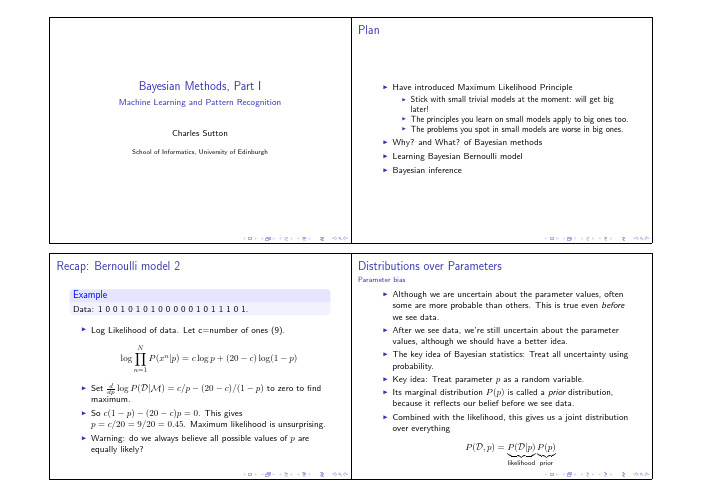
Distributions over Parameters
Parameter bias
log
n=1
P (xn |p) = c log p + (20 − c) log(1 − p)
d Set dp log P (D|M) = c/p − (20 − c)/(1 − p) to zero to ﬁnd maximum.
Bayesian methods involve:
Formulating the prior: Hard because it might be hard to know how to elucidate beliefs or know how to represent beliefs in probabilistic form. Conditioning on data: Computationally hard because after conditioning the posterior distribution might no longer take an easy to represent form. Marginalisation: Computationally hard because the integral might not be analytically tractable and might be hard to approximate.
So c(1 − p) − (20 − c)p = 0. This gives p = c/20 = 9/20 = 0.45. Maximum likelihood is unsurprising. Warning: do we always believe all possible values of p are equally likely?

Nature Research Reporting Summary.pdf_1693203986.4

October 2018Corresponding author(s):Michael P MurphyLast updated by author(s):Mar 15, 2019Reporting SummaryNature Research wishes to improve the reproducibility of the work that we publish. This form provides structure for consistency and transparency in reporting. For further information on Nature Research policies, see Authors & Referees and the Editorial Policy Checklist .StatisticsFor all statistical analyses, confirm that the following items are present in the figure legend, table legend, main text, or Methods section.n/aThe exact sample size (n ) for each experimental group/condition, given as a discrete number and unit of measurement A statement on whether measurements were taken from distinct samples or whether the same sample was measured repeatedlyThe statistical test(s) used AND whether they are one- or two-sided Only common tests should be described solely by name; describe more complex techniques in the Methods section.A description of all covariates tested A description of any assumptions or corrections, such as tests of normality and adjustment for multiple comparisons A full description of the statistical parameters including central tendency (e.g. means) or other basic estimates (e.g. regression coefficient) AND variation (e.g. standard deviation) or associated estimates of uncertainty (e.g. confidence intervals)For null hypothesis testing, the test statistic (e.g. F , t , r ) with confidence intervals, effect sizes, degrees of freedom and P value noted Give P values as exact values whenever suitable.For Bayesian analysis, information on the choice of priors and Markov chain Monte Carlo settingsFor hierarchical and complex designs, identification of the appropriate level for tests and full reporting of outcomesEstimates of effect sizes (e.g. Cohen's d , Pearson's r ), indicating how they were calculatedOur web collection on statistics for biologists contains articles on many of the points above.Software and codePolicy information about availability of computer codeData collection Labsolutions software (Shimadzu, UK)Data analysis XCalibur Qual and and XCalibur Quan Browser software (Thermo Fisher Scientific)BIORAD Quantilife software (BIORAD, UK)'limma' package of R (/packages/release/bioc/html/limma.html)For manuscripts utilizing custom algorithms or software that are central to the research but not yet described in published literature, software must be made available to editors/reviewers. We strongly encourage code deposition in a community repository (e.g. GitHub). See the Nature Research guidelines for submitting code & software for further information.DataPolicy information about availability of dataAll manuscripts must include a data availability statement . This statement should provide the following information, where applicable:- Accession codes, unique identifiers, or web links for publicly available datasets- A list of figures that have associated raw data- A description of any restrictions on data availabilityNearly all data are reported in the manuscript and in the supplemental files. There are no restrictions on data availability. The only original data not in themanuscript is that associated with chemical syntheses and this has been deposited at /10.5525/gla.researchdata.646. In addition the metabolomic data have been uploaded as study MTBLS1085 to MetaboLights (https:///metabolights).October 2018Field-specific reportingPlease select the one below that is the best fit for your research. If you are not sure, read the appropriate sections before making your selection.Life sciencesBehavioural & social sciences Ecological, evolutionary & environmental sciencesFor a reference copy of the document with all sections, see /documents/nr-reporting-summary-flat.pdfLife sciences study design All studies must disclose on these points even when the disclosure is negative.Sample size Pilot experiments, as well as previous work in our laboratories, were used to predict effect size and indicated n=4-8 per group to be sufficient to detect biologically and statistically significant results. No sample size calculations were performed.Data exclusions No data were excluded from the data set.Replication The data were repeated on multiple independent animals. All replicates are true biological (rather than technical) replicates. All replicatiosn were successful.Randomization Animals were randomly allocated to control or treatment groups.Blinding In most cases, detailed in the methods sections, samples were analysed by a blinded observer. It was not possible to apply blinding to the surgical intervention themselves due to the nature of the interventions and the skills required to carry them out.Reporting for specific materials, systems and methodsWe require information from authors about some types of materials, experimental systems and methods used in many studies. Here, indicate whether each material, system or method listed is relevant to your study. If you are not sure if a list item applies to your research, read the appropriate section before selecting a response.Eukaryotic cell linesPolicy information about cell linesCell line source(s)C2C12 mouse myoblasts from American Type Cultute Collection (ATCC) (Middlesex, UK).Authentication Cell line was authenticated as supplied by the commercial vendor. In addition, C2C12 myoblasts were periodicallydifferentiated in to myotubes, in our lab and markers of differentiation identified by western blotting, confirming the identity of the C2C12 cells.Mycoplasma contamination Cell line tested negative for mycoplasma infection in routine tests in the Cambridge MBU tissue culture monly misidentified lines(See ICLAC register)No commonly missidentified cell lines wer used.Animals and other organismsPolicy information about studies involving animals ; ARRIVE guidelines recommended for reporting animal researchLaboratory animals C57BL/6 female mice were purchased from Charles River Laboratories. Mice were maintained in specific-pathogen-free animalfacilities with ad libitum access to food and water. Large white male (Landrace) pigs (45-55 kg) were supplied by Envigo and wereacclimatised for a minimum of 7 days prior to experiments, with ad libitum access to food and water.Wild animals This study did not involve wild animalsField-collected samples This study did not involve animals collected from the fieldEthics oversight All animal experiments were approved by the UK Home Office under the Animals (Scientific Procedures) Act 1986. Mouseexperiments were covered by project license PPL 80/2638 and P7720A3D6. Pig experiments were performed under the HomeOffice Project License held by Envigo.Note that full information on the approval of the study protocol must also be provided in the manuscript.Human research participantsPolicy information about studies involving human research participantsPopulation characteristics Heart biopsies were taken from deceased human DBD donors deemed unsuitable for cardiac transplantation aged 36-69 (TableS1). Informed consent for the use of the human tissue for this project was provided by the donors' families.Recruitment Heart biopsies were taken from deceased human DBD donors deemed unsuitable for cardiac transplantation aged 36-69 (TableS1). Informed consent for the use of the human tissue for this project was provided by the donors' families.Ethics oversight Ethical approval for the studies was obtained from NRES Committee East of England – Cambridge South (REC Reference 15/EE/0152).Note that full information on the approval of the study protocol must also be provided in the manuscript.October 2018。

Bayesian Techniques for Neural Networks- Review and Case Studies

Bayesian Techniques for Neural Networks Review and Case StudiesJouko Lampinen and Aki Vehtari Laboratory of Computational Engineering, Helsinki University of Technology P.O.Box 9400, FIN-02015 HUT, Espoo, Finland E-mail: {mpinen,Aki.Vehtari}@hut.fiABSTRACT We give a short review on Bayesian techniques for neural networks and demonstrate the advantages of the approach in a number of industrial applications. Bayesian approach provides a principled way to handle the problem of overﬁtting, by averaging over all model complexities weighted by their posterior probability given the data sample. The approach also facilitates estimation of the conﬁdence intervals of the results, and comparison to other model selection techniques (such as the committee of early stopped networks) often reveals faulty assumptions in the models. In this contribution we review the Bayesian techniques for neural networks and present comparison results from several case studies that include regression, classiﬁcation, and inverse problems.Possibility to use prior information and hierarchical models for the hyperparameters. Predictive distributions for outputs. In this contribution we demonstrate the advantages of Bayesian MLPs in three case problems. In sections 2 and 3 we give a review of the Bayesian methods for MLP networks. Then we report results on using Bayesian MLP models in regression problem (section 4), tomographic image reconstruction problem (section 5) and classiﬁcation problem (section 6), and compare the approach to standard neural network and other statistical methods.2BAYESIAN APPROACH1INTRODUCTIONIn non-linear function approximation and classiﬁcation, neural networks have become popular tools in recent years. With neural networks the main difﬁculty is in controlling the complexity of the model. It is well known that the optimal number of degrees of freedom in the model depends on the number of training samples, amount of noise in the samples and the complexity of the underlying function being estimated. With standard neural networks techniques the means for both determining the correct model complexity and setting up a network with the desired complexity are rather crude and often computationally very expensive. Another problem of standard neural network methods is the lack of tools for analyzing the results (conﬁdence intervals for the results, like 10 % and 90 % quantiles, etc.). Recently, Bayesian methods have become a viable alternative to the older error minimization based ML (Maximum Likelihood) or MAP (Maximum A Posteriori) approaches [11, 13, 2]. The main advantages of Bayesian multilayer percpetron models are: Automatic complexity control: the values of the regularization coefﬁcients can be selected using only the training data, without the need to use separate training and validation data.The key principle of Bayesian approach is to construct the posterior probability distributions for all the unknown entities in the models. To use the model, marginal distributions are constructed for all those entities that we are interested in, i.e., the end variables of the study. These can be the parameters in parametric models, or the predictions in nonparametric regression or classiﬁcation tasks. Use of the posterior probabilities requires explicit deﬁnition of the prior probabilities for the quantities, as the posterior for a parameter given the data D is according to the Bayes’ rule, p( jD) = p(Dj )p( )=p(D), where p(Dj ) is the likelihood of the parameters and p( ) the prior probability of . The use of the explicit prior information distinguishes the Bayesian approach from the maximum likelihood methods. It is worth noticing that every discrete choice in the model, such as the Gaussian noise model, represents inﬁnite amount of prior information [10]. Any ﬁnite amount of information would not correspond to probability one for, e.g, the Gaussian noise model and probability zero for all the other alternatives. Thus there is large amount of prior information also in the maximum likelihood models (actually it is what separates "good" and "bad" ML models), even though the model parameters are determined solely by the data, to maximize the likelihood p(Djw). In the Bayesian approach there are explicit prior distributions for the model parameters, but asdiscussed above, large part of the prior information is still implicit in the form of the choices made in the model. The marginalization principle leads to complex integrals that cannot be solved in closed form, and thus there are multitude of approaches that differ in the degree of "Bayesianism", that is, how thoroughly this principle is followed. Closest to the ML approach is the Maximum A Posteriori approach, where the posterior distribution is not considered, but the parameters are sought to maximize the posterior probability p(wjD) / p(Djw)p(w), or to minimize the negative log-posterior cost functionBayesian methods can be used for other types of neural networks, like RBF networks, too. Basic MLP model with k outputs isfk (x; w) = wk0 +m X j =1wkj tanh wj0 +d X i=1wji xi ;(1)!E = ? log p(Djw) ? log p(w):The weight decay regularization is an example of this technique. The main drawback of this approach is that it gives no tools for setting the hyperparameters (smoothness coefﬁcients, or model complexity), due to lack of marginalization over these "nuisance parameters". For example, with the Gaussian prior on w, p(w) / exp (? w2 ), the variance term must be set with some external procedure, such as crossvalidation. A further degree of Bayesian principle is utilized in the evidence framework [11], or type II ML approach, where speciﬁc values are estimated for the hyperparameters, so that the marginal probability for the hyperparameters, integrated R over the parameters, p( jD) = p( ; wjD)dw, is maximized. Gaussian approximation is used for the posterior of the parameters, to facilitate closed form marginalization, and thus the resulting posterior is speciﬁed by the mean of the Gaussian approximation. In a full Bayesian approach no ﬁxed values are estimated for any parameters or hyperparameters. If the model is used for prediction, the marginalization is done over the parameters also, as shown in Eq. 4. The priors are then constructed hierarchically, so that the hyperparameters have hyperpriors, and the parameters of those distributions next level priors and so on. See, e.g., [5] for good introduction to these methods. Note again, that in such models there are large amounts of ﬁxed prior knowledge, that is based on uncertain assumptions. So, conceptually, in full hierarchical Bayesian model, no guesses are made for any exact values of the parameters or any smoothness coefﬁcients or other hyperparameters, but guesses are made for the exact forms of their distributions. The goodness of the model depends on these guesses, which in practical applications necessitates using some sort of model validation techniques. This also implies that in practice the Bayesian approach may be more sensitive to the prior assumptions than more classical methods. This is discussed in more detail in chapter 3.7.is a d-dimensional input vector, denotes the where weights, and indices i and j correspond to input and hidden units, respectively. MLP is often considered as a generic semiparametric model, in a sense that there is a large number of parameters without any physical meaning, as in non-parametric models, but the actual model may have very low effective complexity, depending on the complexity of the data, resembling in this respect parametric models with modest number of parameters. Traditionally the complexity of the MLP has been controlled with early stopping or weight decay [2]. In early stopping weights are initialized to small values, so that the sigmoidal hidden units operate on the linear regions and the initial mapping is smooth. Part of the training data is used to train the MLP and the other part is used to monitor the validation error. In the iterative error minimization the training is stopped when the validation error begins to increase, so that the effective complexity may be much less than the number of parameters in the network. The basic early stopping is rather inefﬁcient, as it is very sensitive to the initial conditions of the weights and only part of the available data is used to train the model. These limitations can easily be alleviated by using a committee of early stopping MLPs, with different partitioning of the data to training and stopping sets for each MLP. When used with caution early stopping committee is a good baseline method for MLPs. In weight decay the weights are encouraged to be small by a penalty function, that corresponds to Gaussian prior on the weights, leading to MAP estimate for the model. In practice each layer in the MLP should have different regularization parameter [2], giving the penalty term1xwXj;i2 wji +2Xj;k2 wkj :(2)Problem is how to select good values for i . Traditionally this has been done with cross validation (CV). Since CV gives noisy estimate for error, it does not guarantee that good values for i can be found. Also it easily becomes computationally prohibitive as computational expenses grow exponentially with number of parameters to be selected.3BAYESIAN LEARNING FOR MLP NETWORKS3.2 Bayesian learning 3.1 MLP and model selectionWe concentrate here to one hidden layer MLPs with hyperbolic tangent (tanh) activation function. However, the Consider a regression or classiﬁcation problem involving the prediction of a noisy vector of target variables given the value of a vector of input variables.xyThe process of Bayesian learning is started by deﬁning a model, M, and prior distribution p( ) for the model parameters . After observing new data D = f( (1) ; (1) ); : : : ; ( (n) ; (n) )g, prior distribution is updated to the posterior distribution using Bayes’ rulex yx yp( jD) =p(Dj )p( ) p(D)/ L( jD)p( );(3)where the likelihood function L( jD) gives the probability of the observed data as function of the unknown model parameters. To predict the new output (n+1) for the new input (n+1) , predictive distribution is obtained by integrating the predictions of the model with respect to the posterior distribution of the model parametersUsing classical estimation (error minimization) for the MLP the number of free parameters (weights) in the model need to be adjusted according to the size of the training set, the complexity of the target function and the amount of noise. In Bayesian approach there is no need to restrict the size of the network, but in practice we use modest number of hidden units for computational reasons. In the limit of iniﬁnite number of hidden units the MLP converges to the Gaussian process [13], which is, at least for small sample size, a very viable alternative method.yx3.4 PriorsTypical priors in Bayesian function approximation are smoothing priors, that state, for example, that functions with small second derivative values are more probable. With MLP these lead to a rather complex treatise [8], [1]. As discussed in section 3.1, complexity of the MLP can be controlled, on coarse level, by controlling the size of the weights . This can be achieved by, e.g., Gaussian prior distribution for weights given hyperparameterp(y(n+1) jx(n+1) ; D) = R (n+1) (n+1) p(y jx ; )p( jD)d :(4)This is the same as taking the average prediction of all the models weighted by their posterior probability.ww3.3 Likelihood modelsStatistical model is deﬁned with its likelihood function. If we assume that the n data points ( (i) ; (i) ) are exchangeable we getp(wj ) = (2 )?m=2 m=2 exp(?m X i=1wi2 =2):(9)x yL( jD) =n Y i=1p(y(i) jx(i) ; ):(5)The term p( (i) j (i) ; ) in Eq. (5) depends on our problem. In regression problems, it is generally assumed that the distribution of the target data can be described by a deterministic function of inputs, corrupted by additive Gaussian noise of a constant variance. Probability density for a target yj is theny xThe coarse level of complexity is determined by the hyperparameter , and since we have no speciﬁc knowledge of the right value, we set a vague hyperprior p( ), that merely makes very high and very low values for unprobable. A convenient form for this hyperprior is vague Gamma distribution with mean and shape parameter ap( )Gamma( ; a) / a=2?1 exp(? a=2 ):(10)p(yj jx; w; ) =p 1 exp(? (yj ? fj (x; w)) ); 222 jj2(6)2 where j is the noise variance for the target. See [13] for per-case normal noise variance model and [17] for full covariance model assuming correlating residuals. For a two class classiﬁcation (logistic regression) model, the probability that a binary-valued target, yj , has the value 1 isp(yj = 1jx; w) = 1 + exp(?fj (x; w))]?1(7)and for a many class classiﬁcation (softmax) model, the probability that a class target, y , has value j isp(y = j jx; w) =( w Pexp(fjfx(;x; )) )) : exp( wk k(8)In Eqs. (6), (7) and (8) the function f ( the MLP network.x; w) is in this caseIn order to have a prior for the weights which is invariant under the linear transformations of data, separate priors (each having its own hyperparameters i ) for different weight groups in each layer of a MLP are used [13]. Often very useful prior is called Automatic Relevance Determination (ARD) [12, 13, 14]. In the ARD the input-tohidden weights connected to the same input have common prior variance, and all the variances have common prior distribution (hyperprior). This allows the posterior values for the priors to adjust so that irrelevant inputs have tighter priors and thus those weights are more efﬁciently driven towards zero than with a common prior for all the inputs. For regression models we need also prior for the noise variance in Eq. (6), which is often speciﬁed in terms of corresponding precision, = ?2 . As for , our prior information is usually quite vague, stating that noise variance is not zero nor extremely large. This prior can be expressed with vague Gamma-distribution with mean and shape parameter ap( )Gamma( ; a) / a=2?1 exp(? a=2 ):(11)3.5 PredictionPredictive distribution for new data is obtained by marginalizing (integrating) over the posterior distribution of the parameters and hyperparametersp(y(n+1) jx(n+1) ; D) =Zp(y(n+1) jx(n+1) ; w; ; )p(w; ; jD)dw :(12)We can also evaluate expectations of various functions with respect to the posterior distribution for parameters. For example in regression we may evaluate the expectation for a component of (n+1)^ ykn =( +1)y Zfk (x(n+1) ; w)p(w; ; jD)dw ;When the amount of data increases, the evidence from the data causes the probability mass to concentrate to the smaller area and we need less samples from the posterior distribution. Also less samples are needed to evaluate the mean of the predictive distribution than the tail-quantiles like, 10% and 90% quantiles. So depending on the problem 10–200 samples may be enough for practical purposes. Note that due to autocorrelations in the Markov chain, getting some 100 independent samples from a converged chain may require tens of thousands of samples in the chain, which may require several hours of CPU-time on standard workstation. In our examples (sections 5, 6) we have used Flexible Bayesian Modeling (FBM) software1 , which implements the methods described in [13].(13)3.7 Some modelling issueswhich corresponds to the best guess with squared error loss. The posterior distribution for the parameters p( ; ; jD) is typically very complex, with many modes. Evaluating the integral of Eq. (13) is therefore a difﬁcult task. The integral can be approximated with parametric approximation as in [11] or with numerical approximation as described in next section.w3.6 Markov Chain Monte Carlo methodNeal has introduced an implementation of Bayesian learning for MLPs in which the difﬁcult integration of Eq. (13) is performed using Markov Chain Monte Carlo (MCMC) methods [13]. In [7] there is a good introduction to basic MCMC methods and many applications in statistical data analysis. The integral of Eq. (13) is the expectation of function fk ( (n+1) ; ) with respect to the posterior distribution of the parameters. This and other expectations can be approximated by Monte Carlo method, using a sample of values (t) drawn from the posterior distribution of parametersxww^ ykn( +1)N 1 X f (x(n+1) ; w(t) ): k N t=1(14)Note that samples from the posterior distribution are drawn during the “learning phase” and predictions for new data can be calculated quickly using the same samples and Eq. (14). In the MCMC, samples are generated using a Markov chain that has the desired posterior distribution as its stationary distribution. Difﬁcult part is to create Markov chain which converges rapidly and in which states visited after convergence are not highly dependent. Neal has used the hybrid Monte Carlo (HMC) algorithm [4] for parameters and Gibbs sampling [6] for hyperparameters. HMC is an elaborate Monte Carlo method, which makes efﬁcient use of gradient information to reduce random walk behavior. The gradient indicates in which direction one should go to ﬁnd states with high probability. Use of Gibbs sampling for hyperparameters helps to minimize the amount of tuning that is needed to obtain good performance in HMC.As explained above, the Bayesian approach is based on averaging probable models, where the probability is computed from the chosen distributions for the noise models, parameters etc. Thus the approach may be more sensitive to bad guesses for these distributions than more classical methods, where the model selection is carried out as an external procedure, such as cross-validation that is based on fewer assumptions. In this respect, the Bayesian models can also be overﬁtted in terms of classical model ﬁtting, to produce too complex models and too small posterior estimates for the noise variance. To check the assumptions of the Bayesian models, we always carry out the modelling with simple classical methods (like linear models, early-stopped committees of MLPs, etc.). If the Bayesian model gives inferior results (measured from test set or cross-validated), some of the assumptions are questionable. The following computer simulation elucidates the sensitivity of the Bayesian approach to the correctness of the noise model, compared to the early-stopped committee (ESC). The target function and data are shown in Fig. 1. The modelling test was repeated 100 times with different realizations of Gaussian or Laplacian (double exponential) noise. The model was 1 ? 10 ? 1 MLP with Gaussian noise model. The ﬁgure shows one sample of noise and resulting predictions. The 90% error bars, or conﬁdence intervals, are for the predicted conditional mean of the output given the input, thus the measurement noise is not included in the limits. For the ESC the intervals are simply computed separately for each xvalue from 100 networks. Computing the conﬁdence limits for early-stopped committees is not straightforward, but this very simple ad hoc method often gives similar results as the Bayesian MLP treatment. The summary of the experiment is shown in Table 1. Using classical t-test, the ESC is signiﬁcantly better than the Bayesian model when the noise model is wrong. The Wilcoxon signed rank test also indicated that ESC is better than Bayesian MLP (comparing medians) for Laplacian noise with P-value 0.04. In this simple problem, the both methods are equal for the correct noise model.1 <URL:/˜radford/fbm. software.html>Bayesian MLP 1 Target Data Prediction 90% error bars 1Early−stopped committee Target Data Prediction 90% error bars0.50.500−0.5 −1 −0.5 0 0.5 1 1.5 2−0.5 −1 −0.5 0 0.5 1 1.5 2Figure 1: Test function in demonstrating the sensitivity of Bayesian MLP and Early-stopped committee to the wrong noise model. The ﬁgure shows one sample of noise realization and the resulting predictions, with Bayesian MLP in left and ESC in right ﬁgure. See text for explanation for the error bars.Table 1: Demonstration of the sensitivity of Bayesian MLP and ESC to wrong noise model. For both models the noise model was Gaussian, and the actual noise Gaussian or Laplacian (double explonential). The statistical signiﬁcance of the difference is tested by pairwise t-test, and the shown P-value is the probability of observing equal or larger error in the means if the two methods are equal. The errors are RMS errors of the prediction from the true target function. Signiﬁcance Noise Bayesian MLP ESC of the difference Gaussian 0.278 0.278 0.43 Laplacian 0.283 0.277 0.006amount of cement and water. In the study we had 7 target variables and 19 explanatory variables. Collecting the samples for statistical modeling is rather expensive in this application, as each sample requires preparation of the sand mixture, casting the test pieces and waiting for 91 days for the ﬁnal tests. Thus available samples must be used as efﬁciently as possible, which makes Bayesian techniques a tempting alternative, as they allow ﬁne balance of prior assumptions and evidence from samples. In the study we had 149 samples designed to cover the practical range of the variables, collected by a concrete manufacturing company. MLP networks containing 6 hidden units were used. Different MLP models tested were: MLP ESC : Early stopping committee of 20 MLP networks, with different division of data to training and stopping sets for each member. The networks were initialized to near zero weights to guarantee that the mapping is smooth in the beginning. Bayes MLP : Bayesian MLP with FBM-software, using t-distribution with 4 degrees of freedom as the noise model, vague priors and MCMC-run speciﬁcations similar as used in [13, 14]. 20 networks from the posterior distribution of the network parameters were used. Bayes MLP +ARD: Similar Bayesian MLP to the previous, but using also the ARD prior. Error estimates for predicting the slump are collected in Table 2. Results were insensitive to the exact values of the higher level hyperparameter speciﬁcations as long as the priors were vague, but the use of the structural ARD prior improved the results signiﬁcantly.The implication of this phenomenon in practical applications is, that Bayesian approach usually requires more expert work than the standard approach, to device the reasonable assumptions for the distributions, but that done, the results are in our experience consistently better than with other approaches.4CASE I: REGRESSION TASK IN QUALITY ESTIMATIONIn this section we report results of using Bayesian MLPs for regression in concrete quality estimation problem. The goal of the project was to develop a model for predicting the quality properties of concrete. The quality variables included, e.g., compression strengths and densities for 1, 28 and 91 days after casting, bleeding (water extraction) and spread and slump that measure properties of the fresh concrete. These quality measurements depend on the properties of the stone material (natural or crushed, size and shape distributions of the grains, mineralogical composition), additives, and theRelative change in U100 50 0 5 10 2 15 48 6InjectionFigure 2: Example of the EIT measurement. The simulated bubble formation is bounded by the circles. The current is injected from the electrode with the lightest color and the opposite electrode is grounded. The gray level and the contour curves show the resulting potential ﬁeld.ElectrodeFigure 3: Relative changes in potentials compared to homogeneous background. The eight curves correspond to injections from eight different electrodes.5CASE II: INVERSE PROBLEM IN ELECTRICAL IMPEDANCE TOMOGRAPHYIn this section we report results on using Bayesian MLPs for solving the ill-posed inverse problem in electrical impedance tomography (EIT). The full report of the proposed approach is presented in [9]. The aim in EIT is to recover the internal structure of an object from surface measurements. Number of electrodes are attached to the surface of the object and current patterns are injected from through the electrodes and the resulting potentials are measured. The inverse problem in EIT, estimating the conductivity distribution from the surface potentials, is known to be severely ill-posed, thus some regularization methods must be used to obtain feasible results [15]. Fig. 2 shows a simulated example of the EIT problem. The volume bounded by the circles in the image represent gas bubble ﬂoating in liquid. The conductance of the gas is much lower than that of the liquid, producing the equipotential curves shown in the ﬁgure. Fig. 3 shows the resulting potential signals, from which the image is to be recovered. In [9] we proposed a novel feedforward solution for the reconstruction problem. The approach is based on computing the principal component decomposition for the potential signals and the eigenimages of the bubble distribution from theFigure 4: Example of image reconstructions with MLP ESC (upper row) and the Bayesian MLP (lower row)Table 2: Ten fold cross-validation error estimates for predicting the slump of concrete. Method MLP ESC Bayes MLP Bayes MLP +ARD Root mean square error37 34 27autocorrelation model of the bubbles. The input to the MLP is the projection of the potential signals to the ﬁrst principal components, and the MLP gives the coefﬁcients for reconstructing the image as weighted sum of the eigenimages. The projection of the potentials and the images to the eigenspace reduces correlations from the input and the output data of the network and detaches the actual inverse problem from the representation of the potential signals and image data. The reconstruction was based on 20 principal components of the 128 dimensional potential signal and 30 eigenimages with resolution 41 41 pixels. The training data consisted of 500 simulated bubble formations with one to ten overlapping circular bubbles in each image. To compute the reconstructions MLPs containing 30 hidden units were used. Models tested were MLP ESC and Bayes MLP (see section 4). Because of the input projection, ARD prior should not make much difference in results (this was veriﬁed in preliminary tests), and so model with ARD prior was not used in full tests. We also compared results to TV-inverse method, which is a state-of-the-art inverse method based on iterative inversion of the forward model with total variation regularization. Fig. 4 shows examples of the image reconstruction results. Table 3 shows the quality of the image reconstructions withTable 3: Errors in reconstructing the bubble shape and estimating the void fraction from the reconstructed images. See text for explanation of the models. Classiﬁcation error % TV-inverse 9.7 MLP ESC 6.7 Bayes MLP 5.9 Method Relative Rel. error in error in VF direct VF % % 22.8 8.7 3.8 8.1 3.4Table 4: CV error estimates for forest scene classiﬁcation. See text for explanation of the different models.Error%KNN LOOCV CART MLP ESC Bayes MLP Bayes MLP +ARD 20 30 13 12 110.50.4 Void fraction, guess0.30.20.10.10.2 0.3 Void fraction, target0.40.5Figure 5: Scatterplot of the void fraction estimate with 10% and 90% quantiles.models, measured by error in the void fraction and percentage of erroneous pixels in the segmentation, over the test set. An important goal in this process tomography application was to estimate the void fraction, which is the proportion of gas and liquid in the image. With the proposed approach such goal variables can be estimated directly without explicit reconstruction of the image. The last column in Table 3 shows the relative absolute error in estimating the void fraction directly from the projections of the potential signals. With Bayesian methods we can easily calculate conﬁdence intervals for outputs. Fig. 5 shows the scatter plot of the void fraction versus the estimate by the Bayesian MLP. The 10% and 90% quantiles are computed directly from the posterior distribution of the model output. See [9] for results for effect of additive Gaussian noise to the performance of the method.Forest scene classiﬁcation task is demanding due to the texture richness of the trees, occlusions of the objects and diverse lighting conditions under operation. This makes it difﬁcult to determine which are optimal image features for the classiﬁcation. One way to proceed is to extract many different types of potentially suitable features. In [16] we extracted total of 84 statistical and Gabor-ﬁlter based features over different size windows at each spectral channel. Due to the large number of features, many classiﬁer methods would suffer from the curse of dimensionality, but the Bayesian MLP managed well in the high dimensional problem. Total of 48 images were collected by using an ordinary digital camera in varying weather conditions. The labeling of the image data was done by hand via identifying many types of tree and background image blocks with different textures and lighting conditions. In this study only pines were considered. To estimate classiﬁcation errors of different methods we used eight-fold cross-validation error estimate, i.e., 42 of 48 pictures were used for training and the six left out for error evaluation, and this scheme was repeated eight times. In addition to 20 hidden unit MLP models MLP ESC and Bayesian MLP (see section 5) the models tested were: KNN LOOCV : K-nearest-neighbor, where K is chosen by leave-one-out cross-validation. CART : Classiﬁcation And Regression Tree [3]. Bayesian MLP +ARD : Same as Bayesian MLP plus using Automatic Relevance Determination prior. CV error estimates are collected in Table 4. Fig. 6 shows example image classiﬁed with different methods.7SUMMARY6CASE III: CLASSIFICATION TASK IN FOREST SCENE ANALYSISIn this section we report results of using Bayesian MLP for classiﬁcation of forest scenes, to accurately recognize and locate the trees from any background.The reviewed case problems in real applications illustrate the advantages of Bayesian MLPs. The approach contains automatic complexity control, as in the Bayesian inference all the results are conditioned on the individual training sample available. Thus the complexity is matched to the support that the training data carries for the models. In addition, the Bayesian approach gives the predictive distributions for the outputs, which can be used to estimate the reliability of the。

1、下载文档前请自行甄别文档内容的完整性，平台不提供额外的编辑、内容补充、找答案等附加服务。
2、"仅部分预览"的文档,不可在线预览部分如存在完整性等问题,可反馈申请退款(可完整预览的文档不适用该条件!)。
3、如文档侵犯您的权益，请联系客服反馈,我们会尽快为您处理(人工客服工作时间：9:00-18:30)。

temperature used for the training of the ANN has been proposed in [9], while both linear and non-linear terms were adopted by the ANN structure. Due to load curve periodicity, a non-fully connected ANN consisting of one main and three supporting neural networks has been used [10] to incorporate input variables like the day of the week, the hour of the day and temperature. Various methods were proposed to accelerate the ANN training [11], while the structure of the network has been proved to be system depended [12]. The most recent proposed ANN models for STLF tune the model performance efficiency based on the practical experience gained by the model implementation to Energy Management Systems (EMS), [13, 14, 15]. Hybrid neuro-fuzzy systems applications to STLF have appeared recently. Such methods synthesize fuzzy-expert systems and ANN techniques to yield impressive results, as reported in [16, 17]. Each of the methods discussed above has its own advantages and shortcomings. Our own experience is that no single predictor type is universally best. For example, an ANN predictor may give more accurate load forecasts during morning hours, while a LR predictor may be superior for evening hours. Hence, a method that combines various different types of predictors may outperform any single “pure” predictor of the types discussed above. In this paper we present such a “combination” STLF method, the so called Bayesian Combined Predictor (BCP), which utilizes conditional probabilities and Bayes’ rule to combine ANN and LR predictors [18, 19, 23]. We proceed to describe the “pure” LR and ANN predictors and the BCP combination method. Then we present results and statistics of BCP forecasts for the Greek Public Power Corporation (PPC) dispatch center of the island of Crete during 1994. 2. STLF USING “PURE” PREDICTORS
make use of statistical models, expert systems or artificial neural networks (ANN); in addition the hybrid method of fuzzy neural networks has appeared in the bibliography recently. Statistical STLF models can be generically separated into regression models [1] and time series models [2]; both can be either static or dynamic. In static models, the load is considered to be a linear combination of time functions, while the coefficients of these functions are estimated through linear regression or exponential smoothing techniques [3]. In dynamic models weather data and random effects are also incorporated since autoregressive moving average (ARMA) models are frequently used. In this approach the load forecast value consists of a deterministic component that represents load curve periodicity and a random component that represents deviations from the periodic behavior due to weather abnormalities or random correlation effects. An overview over different statistical approaches to the STLF problem can be found in [4]. The most common (and arguably the most efficient) statistical predictors apply a linear regression on past load and temperature data to forecast future load. For such predictors, we will use the generic term Linear Regression (LR) predictors. Expert systems have been successfully applied to STLF [5, 6]. This approach, however, presumes the existence of an expert capable of making accurate forecasts who will train the system. The application of artificial neural networks to STLF yields encouraging results; a discussion can be found in [7]. The ANN approach does not require explicit adoption of a functional relationship between past load or weather variables and forecasted load. Instead, the functional relationship between system inputs and outputs is learned by the network through a training process. Once training has been completed, current data are input to the ANN, which outputs a forecast of tomorrow's hourly load. One of the first neural-network-based STLF models was a three-layer neural network used to forecast the next hour load [8]. A minimum-distance based identification of the appropriate historical patterns of load and
A BAYESIAN COMBINATION METHOD FOR SHORT TERM LOAD FORECASTING
A. BAKIRTZIS, S. KIARTZIS, V. PETRIDIS AND A. KEHAGIAS Department of Electrical and Computer Engineering Aristotle University of Thessaloniki, Greece Abstract: This paper presents the Bayesian Combined Predictor (BCP), a probabilistically motivated predictor for Short Term Load Forecasting (STLF) based on the combination of an artificial neural network (ANN) predictor and two linear regression (LR) predictors. The method is applied to STLF for the Greek Public Power Corporation dispatching center of the island of Crete, using 1994 data, and daily load profiles are obtained. Statistical analysis of prediction errors reveals that during given time periods the ANN predictor consistently forecasts better for certain hours of the day, while the LR predictors forecast better during for the rest. This relative prediction advantage may change over different time intervals. The combined prediction is a weighted sum of the ANN and LR predictions, where the weights are computed using an adaptive update of the Bayesian posterior probability of each predictor, based on their past predictive performance. The proposed method outperforms both ANN and LR predictions. This paper appeared in Electrical Power and Energy Systems, Vol.19, pp.171-177, 1997 1. INTRODUCTION The formulation of economic, reliable and secure operating strategies for a power system requires accurate short term load forecasting (STLF). The principal objective of STLF is to provide load predictions for the basic generation scheduling functions, the security assessment of a power system and for dispatcher’s information. A large number of computational techniques have been used for the solution of the STLF problem; these