Euler–Lagrange equation

Euler–Lagrange_equation

Euler–Lagrange equationJump to: navigation, searchIn calculus of variations, the Euler–Lagrange equation, or Lagrange's equation, is a differential equation whose solutions are the functions for which a given functional is stationary. It was developed by Swiss mathematician Leonhard Euler and Italian mathematician Joseph Louis Lagrange in the 1750s.Because a differentiable functional is stationary at its local maxima and minima, the Euler–Lagrange equation is useful for solving optimization problems in which, given some functional, one seeks the function minimizing (or maximizing) it. This is analogous to Fermat's theorem in calculus, stating that where a differentiable function attains its local extrema, its derivative is zero.In Lagrangian mechanics, because of Hamilton's principle of stationary action, the evolution of a physical system is described by the solutions to the Euler–Lagrange equation for the action of the system. In classical mechanics, it is equivalent to Newton's laws of motion, but it has the advantage that it takes the same form in any system of generalized coordinates, and it is better suited to generalizations (see, for example, the "Field theory" section below).HistoryThe Euler–Lagrange equation was developed in the 1750s by Euler and Lagrange in connection with their studies of the tautochrone problem. This is the problem of determining a curve on which a weighted particle will fall to a fixed point in a fixed amount of time, independent of the starting point.Lagrange solved this problem in 1755 and sent the solution to Euler. The two further developed Lagrange's method and applied it to mechanics, which led to the formulation of Lagrangian mechanics. Their correspondence ultimately led to the calculus of variations, a term coined by Euler himself in 1766.[1]StatementThe Euler–Lagrange equation is an equation satisfied by a function q of a real argument t which is a stationary point of the functionalwhere:∙q is the function to be found:such that q is differentiable, q(a) = x a, and q(b) = x b;∙q′ is the derivative of q:TX being the tangent bundle of X (the space of possible values of derivatives of functions with values in X);∙L is a real-valued function with continuous first partial derivatives:The Euler–Lagrange equation, then, is the ordinary differential equationwhere L x and L v denote the partial derivatives of L with respect to the second and third arguments, respectively.If the dimension of the space X is greater than 1, this is a system of differential equations, one for each component:Derivation of one-dimensionalEuler-Lagrange equationAlternate derivation of one-dimensionalEuler-Lagrange equationExamplesA standard example is finding the real-valued function on the interval[a , b ], such that f (a ) = c and f (b ) = d , the length of whose graph is as short as possible. The length of the graph of f is:the integrand function being 2'1)',,(y y y x L += evax , y , y ′)= (x , f (x ), f ′(x )).The partial derivatives of L are:By substituting these into the Euler –Lagrange equation, we obtainthat is, the function must have constant first derivative, and thus its graph is a straight line .Classical mechanicsBasic methodTo find the equations of motions for a given system, one only has to follow these steps:∙From the kinetic energy T, and the potential energy V, compute the Lagrangian L = T−V.∙Compute .∙Compute and from it, . It is important that be treated as a complete variable in its own right, and not as a derivative.∙Equate . This is, of course, the Euler–Lagrange equation.∙Solve the differential equation obtained in the preceding step. At this point, is treated "normally". Note that the above might bea system of equations and not simply one equation.Particle in a conservative force fieldThe motion of a single particle in a conservative force field (for example, the gravitational force) can be determined by requiring the action to be stationary, by Hamilton's principle. The action for this system iswhere x(t) is the position of the particle at time t. The dot above is Newton's notation for the time derivative: thus ẋ(t) is the particle velocity, v(t). In the equation above, L is the Lagrangian (the kinetic energy minus the potential energy):where:∙m is the mass of the particle (assumed to be constant in classical physics);∙v i is the i-th component of the vector v in a Cartesian coordinate system (the same notation will be used for other vectors);U is the potential of the conservative force.In this case, the Lagrangian does not vary with its first argument t. (By Noether's theorem, such symmetries of the system correspond to conservation laws. In particular, the invariance of the Lagrangian with respect to time implies the conservation of energy.)By partial differentiation of the above Lagrangian, we find:where the force is F = −∇U (the negative gradient of the potential, by definition of conservative force), and p is the momentum. By substituting these into the Euler–Lagrange equation, we obtain a system of second-order differential equations for the coordinates on the particle's trajectory,which can be solved on the interval [t0, t1], given the boundary values x(t0) and x i(t1). In vector notation, this system readsior, using the momentum,which is Newton's second law.Field theoryThis section contains too much jargon and may need simplification or further explanation. Please discuss this issue on the talk page, and/or remove or explain jargon terms used in the article. Editing help is available. (December 2009)Field theories, both classical field theory and quantum field theory, deal with continuous coordinates, and like classical mechanics, has its own Euler–Lagrange equation of motion for a field,where∙is the field, and∙is a vector differential operator:Note: Not all classical fields are assumed commuting/bosonic variables, (like the Dirac field, the Weyl field, the Rarita-Schwinger field) are fermionic and so, when trying to get the field equations from the Lagrangian density, one must choose whether to use the right or the left derivative of the Lagrangian density (which is a boson) with respect to the fields and their first space-time derivatives which arefermionic/anticommuting objects.There are several examples of applying the Euler–Lagrange equation to various Lagrangians:∙Dirac equation;∙Proca equation;∙electromagnetic tensor;∙Korteweg–de Vries equation;∙quantum electrodynamics.Variations for several functions, several variables, and higher derivativesSingle function of single variable with higher derivatives The stationary values of the functionalcan be obtained from the Euler-Lagrange equation[2]Several functions of one variableIf the problem involves finding several functions () of a single independent variable (x) that define an extremum of the functionalthen the corresponding Euler-Lagrange equations are[2]Single function of several variablesA multi-dimensional generalization comes from considering a function on n variables. If Ω is some surface, thenis extremized only if f satisfies the partial differential equationWhen n = 2 and is the energy functional, this leads to the soap-film minimal surface problem.Several functions of several variablesIf there are several unknown functions to be determined and several variables suchtthe system of Euler-Lagrange equations is[2]Single function of two variableswith higher derivativesIf there is a single unknown functionto be determined that is dependent ontwo variables and their higherderivatives such thatthe Euler-Lagrange equation is[2]Notes1.^ A short biography of Lagrange2.^ a b c d Courant, R. and Hilbert, D., 1953, Methods of Mathematical Physics:Vol I, Interscience Publishers, New York.References∙Weisstein, Eric W., "Euler-Lagrange Differential Equation" from MathWorld.∙Calculus of Variations on PlanetMath∙Izrail Moiseevish Gelfand (1963). Calculus of Variations. Dover.ISBN0-486-41448-5.∙Calculus of Variations at Example (Provides examples of problems from the calculus of variations that involve theEuler–Lagrange equations.)。

广义euler-lagrange方程

广义euler-lagrange方程全文共四篇示例，供读者参考第一篇示例：广义Euler-Lagrange方程是经典力学中一个非常重要的数学工具，它是描述自然系统中最优路径的数学原理。

Euler-Lagrange方程最初由拉格朗日(Lagrange)在18世纪提出，用于描述质点在空间中的运动轨迹。

而广义Euler-Lagrange方程则是将这一原理推广到更一般的情况，包括多自由度系统以及约束系统。

在力学体系中，广义坐标q和广义速度q̇被用来描述系统的状态。

系统的能量函数，也就是Lagrange函数L(q, q̇, t)可以表示为广义坐标、广义速度和时间的函数。

广义Euler-Lagrange方程可以写作：∂L/∂q - d/dt(∂L/∂q̇) = 0这个方程描述了系统在任何可能的广义坐标和广义速度下的运动方程。

这个方程可以通过对Lagrange函数求取拉格朗日方程而得到，也是系统的动力学方程之一。

这个方程表明，在一个势场中，系统沿着使拉格朗日函数L最小的路径运动。

广义Euler-Lagrange方程是经典力学中一个非常重要的数学工具，它描述了系统在任何广义坐标和广义速度下的运动方程。

这个方程是系统动力学的基础，通过它可以揭示系统的演化规律，对系统的研究和分析起着至关重要的作用。

在未来的研究中，广义Euler-Lagrange方程将继续发挥重要的作用，为我们理解物理世界提供更深入的洞察。

第二篇示例：广义Euler-Lagrange方程是控制理论中一种重要的数学工具，用于描述动力系统的运动方程。

它是拉格朗日动力学的推广，适用于广义坐标和广义速度的情况。

在经典力学中，我们常常使用拉格朗日方程来描述系统的运动。

拉格朗日方程给出了系统的运动方程，通过最小作用原理可以推导出系统的运动轨迹。

但是拉格朗日方程只能描述质点在经典力学中的运动，对于更一般的情况，比如多自由度系统或者约束系统，就需要使用广义Euler-Lagrange方程。

变分原理推导拉格朗日方程

变分原理推导拉格朗日方程变分原理及拉格朗日方程简介在物理学中，拉格朗日方程是一种描述物体运动规律的方程，它源于变分原理。

变分原理是一种数学工具，用于研究力学系统中物体运动的最优化问题。

本文将详细介绍变分原理的推导过程，以及如何得到拉格朗日方程。

一、变分原理概述变分原理是基于欧拉-拉格朗日方程（Euler-Lagrange equation）的一种数学原理，它广泛应用于力学、物理学和工程领域。

欧拉-拉格朗日方程描述了一个物体在受力作用下的运动状态，其中的拉格朗日量（Lagrangian）是与物体运动状态有关的标量函数。

二、变分原理推导拉格朗日方程1.设定问题：首先，我们需要明确研究的问题。

假设我们研究一个N维空间的质点，在受力F作用下的运动。

质点的位移为q，速度为v。

2.构造拉格朗日量：为了描述质点的运动状态，我们需要构造一个拉格朗日量L。

拉格朗日量是位移q和速度v的函数，即L(q, v)。

3.计算泛函：泛函是拉格朗日量关于位移和速度的偏导数之和。

对于给定的拉格朗日量L，我们可以计算其关于位移和速度的偏导数，然后将它们相加得到泛函J。

泛函J =∫(L(q, v) dt)4.求极值：为了找到质点的运动规律，我们需要求解泛函J的极值。

求极值的方法是求解欧拉方程，即泛函J关于位移和速度的偏导数等于0。

∂J/∂q =0∂J/∂v =05.求解运动方程：将欧拉方程求解得到质点的运动方程，即拉格朗日方程。

三、拉格朗日方程的应用拉格朗日方程可以描述质点、刚体、弹性体等各种力学系统的运动规律。

通过求解拉格朗日方程，我们可以得到物体在给定力作用下的位移、速度和加速度等物理量。

此外，拉格朗日方程还可以应用于控制理论、优化算法等领域。

总结通过变分原理，我们可以推导出拉格朗日方程，从而描述力学系统中物体的运动规律。

拉格朗日方程在物理学、工程学和控制理论等领域具有广泛的应用价值。

了解变分原理及其推导过程，有助于我们更好地理解拉格朗日方程，并在实际问题中发挥其重要作用。

欧拉-拉格朗日方程

欧拉-拉格朗日方程【概述】欧拉−拉格朗日方程（Euler−Lagrange Equation）又称为Lagrange变分法，是一个重要的数学方程。

是由著名数学家Euler和Lagrange共同发现的。

它提供了一种简便有效的方法来求解多元复杂的函数的极大或极小值。

欧拉-拉格朗日方程实际上是也被称作动力系统的微分方程的一种表示形式【原理】欧拉-拉格朗日方程是一条带微分的方程，它是由拉格朗日变分法推出的，其形式如下：$$\frac{\delta\Psi}{\delta y_i}=0$$其中，$y_i$是需要求导的函数的变量；$\Psi$是不可微的函数，它是拉格朗日函数，也叫做动作函数。

具体地说，拉格朗日变分法要求最后计算出的函数值极大时其微分值应该为零，这样就可以使函数值朝着极大值方向变动，而拉格朗日函数记录了变分值之间的微分值大小以及函数变动的方向，因而可以推出欧拉-拉格朗日方程来求解函数本身的极大值或者极小值。

【优点】(1) 欧拉-拉格朗日方程可以不断调整变量，改变函数值，以达到求对对函数的极大值的极小值的目的。

(2) 求解欧拉-拉格朗日方程时涉及到微积分，可以简化解题步骤，省去需要繁琐的推导步骤，从而节省时间。

(3) 此方法可以有效地解决多元变量和复杂函数问题，有效提高解算精度。

【应用】(1) 力学中，欧拉-拉格朗日方程用来求解极小总动量及极小流体效率等。

(2) 工程中，用欧拉-拉格朗日方程来求解某种参数取得某种最佳效果的优化方程。

(3) 电子工程中，欧拉-拉格朗日方程可以用来求解电子电路中、集成电路中最优参数计算问题。

(4) 生物学中，欧拉-拉格朗日方程在对一定植物对环境适应度进行优化时可以得到很好的应用。

欧拉拉格朗日方程小时百科

欧拉-拉格朗日方程什么是欧拉-拉格朗日方程欧拉-拉格朗日方程（Euler-Lagrange equation）是经典力学中的一个重要定律，用于描述质点或系统在势能场中的运动。

它由瑞士数学家欧拉和法国数学家拉格朗日在18世纪中叶独立提出，并成为经典力学的基础之一。

欧拉-拉格朗日方程可以从变分原理（principle of least action）推导而来，该原理认为自然界中的运动路径是使作用量（action）取极小值的路径。

作用量定义为质点或系统在一段时间内所受到的所有力所做的功之和。

欧拉-拉格朗日方程的表达式对于一个质点或系统，在广义坐标q i和广义速度q̇i下，其动能T和势能V可以表示为：T=T(q1,q2,…,q n,q̇1,q̇2,…,q̇n)V=V(q1,q2,…,q n)其中n表示系统自由度的数量。

根据变分原理，作用量可以表示为：S=∫Lt2t1(q1,q2,…,q n,q̇1,q̇2,…,q̇n)dt其中L=T−V称为拉格朗日函数（Lagrangian），它是动能和势能的差。

欧拉-拉格朗日方程可以通过对作用量进行变分，使其取极值，得到：∂L ∂q i −ddt(∂L∂q̇i)=0对于每一个广义坐标q i，都有一个对应的欧拉-拉格朗日方程。

这些方程描述了系统在广义坐标和时间上的运动规律。

欧拉-拉格朗日方程的意义与应用欧拉-拉格朗日方程是经典力学的重要工具，它具有以下几个重要意义和应用：1. 简化运动方程相比于牛顿力学中的运动方程，欧拉-拉格朗日方程更加简洁、优雅，并且适用于复杂系统。

通过引入广义坐标和广义速度，可以将系统的自由度从直角坐标系中解放出来，从而简化了运动方程的表达。

2. 描述约束系统在经典力学中，约束系统是指由于各种限制条件而使得系统自由度减少的情况。

欧拉-拉格朗日方程可以很好地描述约束系统的运动，通过引入拉格朗日乘子（Lagrange multiplier）来处理约束条件。

Euler–Lagrange equationFrom Wikipedia, the free encyclopediaJump to: navigation, searchIn calculus of variations, the Euler–Lagrange equation, or Lagrange's equation, is a differential equation whose solutions are the functions for which a given functional is stationary. It was developed by Swiss mathematician Leonhard Euler and Italian mathematician Joseph Louis Lagrange in the 1750s.Because a differentiable functional is stationary at its local maxima and minima, the Euler–Lagrange equation is useful for solving optimization problems in which, given some functional, one seeks the function minimizing (or maximizing) it. This is analogous to Fermat's theorem in calculus, stating that where a differentiable function attains its local extrema, its derivative is zero.In Lagrangian mechanics, because of Hamilton's principle of stationary action, the evolution of a physical system is described by the solutions to the Euler–Lagrange equation for the action of the system. In classical mechanics, it is equivalent to Newton's laws of motion, but it has the advantage that it takes the same form in any system of generalized coordinates, and it is better suited to generalizations (see, for example, the "Field theory" section below).Contents1 History∙ 2 Statement∙ 3 Exampleso 3.1 Classical mechanics▪ 3.1.1 Basic method▪ 3.1.2 Particle in a conservative force field o 3.2 Field theory∙ 4 Variations for several functions, several variables, and higher derivativeso 4.1 Single function of single variable with higherderivativeso 4.2 Several functions of one variableo 4.3 Single function of several variableso 4.4 Several functions of several variableso 4.5 Single function of two variables with higher derivatives ∙ 5 Notes∙ 6 References∙7 See alsoHistoryThe Euler–Lagrange equation was developed in the 1750s by Euler and Lagrange in connection with their studies of the tautochrone problem. This is the problem of determining a curve on which a weighted particle will fall to a fixed point in a fixed amount of time, independent of the starting point.Lagrange solved this problem in 1755 and sent the solution to Euler. The two further developed Lagrange's method and applied it to mechanics, which led to the formulation of Lagrangian mechanics. Their correspondence ultimately led to the calculus of variations, a term coined by Euler himself in 1766.[1]StatementThe Euler–Lagrange equation is an equation satisfied by a function q of a real argument t which is a stationary point of the functionalwhere:∙q is the function to be found:such that q is differentiable, q(a) = x a, and q(b) = x b;∙q′ is the derivative of q:TX being the tangent bundle of X (the space of possible values of derivatives of functions with values in X);L is a real-valued function with continuous first partial derivatives:The Euler–Lagrange equation, then, is the ordinary differential equationwhere L x and L v denote the partial derivatives of L with respect to the second and third arguments, respectively.If the dimension of the space X is greater than 1, this is a system of differential equations, one for each component:Derivation of one-dimensionalEuler-Lagrange equationAlternate derivation of one-dimensionalEuler-Lagrange equationExamplesA standard example is finding the real-valued function on the interval [a, b], such that f(a) = c and f(b) = d, the length of whose graph is as short as possible. The length of the graph of f is:the integrand function being 2'1)',,(y y y x L += evax , y , y ′)= (x , f (x ), f ′(x )).The partial derivatives of L are:By substituting these into the Euler –Lagrange equation, we obtainthat is, the function must have constant first derivative, and thus its graph is a straight line .Classical mechanicsBasic methodTo find the equations of motions for a given system, one only has to follow these steps:∙ From the kinetic energy T , and the potential energy V , compute the Lagrangian L = T − V .∙ Compute .∙ Compute and from it, . It is important that be treated as a complete variable in its own right, and not as a derivative. ∙ Equate. This is, of course, the Euler –Lagrange equation.∙Solve the differential equation obtained in the preceding step. At this point, is treated "normally". Note that the above might bea system of equations and not simply one equation.Particle in a conservative force fieldThe motion of a single particle in a conservative force field (for example, the gravitational force) can be determined by requiring the action to be stationary, by Hamilton's principle. The action for this system iswhere x(t) is the position of the particle at time t. The dot above is Newton's notation for the time derivative: thus ẋ(t) is the particle velocity, v(t). In the equation above, L is the Lagrangian (the kinetic energy minus the potential energy):where:∙m is the mass of the particle (assumed to be constant in classical physics);∙v i is the i-th component of the vector v in a Cartesian coordinate system (the same notation will be used for other vectors);∙U is the potential of the conservative force.In this case, the Lagrangian does not vary with its first argument t. (By Noether's theorem, such symmetries of the system correspond to conservation laws. In particular, the invariance of the Lagrangian with respect to time implies the conservation of energy.)By partial differentiation of the above Lagrangian, we find:where the force is F = −∇U (the negative gradient of the potential, by definition of conservative force), and p is the momentum. By substitutingthese into the Euler–Lagrange equation, we obtain a system of second-order differential equations for the coordinates on the particle's trajectory,which can be solved on the interval [t0, t1], given the boundary values x(t0) and x i(t1). In vector notation, this system readsior, using the momentum,which is Newton's second law.Field theoryThis section contains too much jargon and may need simplification or further explanation. Please discuss this issue on the talk page, and/or remove or explain jargon terms used in the article. Editing help is available. (December 2009)Field theories, both classical field theory and quantum field theory, deal with continuous coordinates, and like classical mechanics, has its own Euler–Lagrange equation of motion for a field,where∙is the field, and∙is a vector differential operator:Note: Not all classical fields are assumed commuting/bosonic variables, (like the Dirac field, the Weyl field, the Rarita-Schwinger field) are fermionic and so, when trying to get the field equations from the Lagrangian density, one must choose whether to use the right or the left derivative of the Lagrangian density (which is a boson) with respect to the fields and their first space-time derivatives which arefermionic/anticommuting objects.There are several examples of applying the Euler–Lagrange equation to various Lagrangians:∙Dirac equation;∙Proca equation;∙electromagnetic tensor;∙Korteweg–de Vries equation;∙quantum electrodynamics.Variations for several functions, several variables, and higher derivativesSingle function of single variable with higher derivatives The stationary values of the functionalcan be obtained from the Euler-Lagrange equation[2]Several functions of one variableIf the problem involves finding several functions () of a single independent variable (x) that define an extremum of the functionalthen the corresponding Euler-Lagrange equations are[2]Single function of several variablesA multi-dimensional generalization comes from considering a function on n variables. If Ω is some surface, thenis extremized only if f satisfies the partial differential equationWhen n = 2 and is the energy functional, this leads to the soap-film minimal surface problem.Several functions of several variablesIf there are several unknown functions to be determined and several variables such thatthe system of Euler-Lagrange equations is[2]Single function of two variables with higher derivativesIf there is a single unknown function to be determined that is dependent on two variables and their higher derivatives such thatthe Euler-Lagrange equation is[2]Notes1.^ A short biography of Lagrange2.^ a b c d Courant, R. and Hilbert, D., 1953, Methods of Mathematical Physics:Vol I, Interscience Publishers, New York.References∙Weisstein, Eric W., "Euler-Lagrange Differential Equation" from MathWorld.∙Calculus of Variations on PlanetMath∙Izrail Moiseevish Gelfand (1963). Calculus of Variations. Dover.ISBN0-486-41448-5.∙Calculus of Variations at Example (Provides examples of problems from the calculus of variations that involve theEuler–Lagrange equations.)See also∙Lagrangian mechanics∙Hamiltonian mechanics∙Analytical mechanics∙Beltrami identity。

euler-lagrange方程

euler-lagrange方程
什么是欧拉 - 拉格朗日方程？
1. 欧拉 - 拉格朗日方程是一类非线性微分方程，用来研究动力系统。

2. 欧拉 - 拉格朗日方程又称为动力学方程，是构成动力系统解析解决方案的重要部分。

3. 欧拉 - 拉格朗日方程是一种重要的常微分方程，它描述了物理系统在某一特定状态下的运动状态。

4. 欧拉 - 拉格朗日方程就是一类关于变分的求解的问题的重要工具，又被称为确定动力学机理的一种方法。

5. 欧拉 - 拉格朗日方程可用来研究非线性系统，例如热力学系统、力学系统等，用来寻求满足最坏情况下的最优解。

6. 欧拉 - 拉格朗日方程建立了力学系统运动的微不平衡状态的基础，也断定量变的话，系统能够达到最低能量状态。

7. 欧拉 - 拉格朗日方程具有普遍适用性，可以用来描述包括生物动力系
统在内的复杂的系统的运动状态，当力学系统有多个自由度时，欧拉 - 拉格朗日方程也可以被应用。

欧拉运动方程

欧拉运动方程
欧拉运动方程（Euler’s Equation of Motion）是一种用于描述物体的运动方程，它可以用来表示物体在特定时刻的加速度与力之间的关系。

它也被称为欧拉-Lagrange 方程，因为它同时引用了欧拉和Lagrange的概念。

欧拉运动方程是一种常用的力学方程，它可以用来描述物体运动的性质。

它是由十九世纪德国数学家Leonhard Euler在1750年发现的，他用它来描述物体在特定时刻的加速度与力之间的关系。

欧拉运动方程可以有多种形式，但其基本原理都是相同的。

它的一般形式如下：
F=ma+v×dv/dt
其中，F是物体上的所有力的合力，m是物体的质量，a是物体的加速度，v是物体的速度，dv/dt是物体速度的变化率。

从上面可以看出，欧拉运动方程将物体的运动分解为力和加速度。

根据物理学原理，力是物体加速度的原因，而加速度是物体速度的变化率。

因此，欧拉运动方程可以用来描述物体的运动，因为它可以表示物体运动的力与加速度之间的关系。

欧拉运动方程有许多用途，它可以用来解决物体运动的问题，包括物体在特定力作用下的运动、物体在多个力作用下的运动、物体在三维空间中的运动等等。

它也可以用来描述物体在地理空间中的运动，以及物体在引力场中的运动。

此外，欧拉运动方程还可以用来解决热力学问题，即物体在不同温度下的运动问题，这对于研究物体的运动性能特别有用。

欧拉运动方程是一种重要的力学方程，它可以用来解决有关物体力学运动的问题，广泛应用于物理、力学和工程领域。

它是一种重要的理论基础，可以用来解决许多有关物体运动的实际问题。

Euler-Lagrange equations

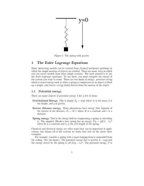
Figure 1:The spring with gravity1The Euler Lagrange Equations Many interesting models can be created from classical mechanics problems in which the simple motions of objects are studied.There are many ways in which you can create models from these simple systems.The most general is to use the Euler-Lagrange equations.To use these,you must compute the energy of the system you want to study.There are two kinds of energy:potential energy which is stored energy such as when a spring is compressed or an object is lifted up a height;and kinetic energy which derives from the motion of the object.1.1Potential energy.There are many sources of potential energy.I list a few of them:Gravitational Energy.This is simply E g =mgh where m is the mass,h isthe height,and g is gravity.Inverse distance energy.Many phenomena have energy that depends ofthe inverse of the distance,E i =K/r where K is a constant and r is a distance.Spring energy.This is the energy held by compressing a spring or extendingit.The simplest (Hooke’s law)spring has an energy,E H =1Chemical and electricalcations,but almost all examples.F or example,consid theceiling.(See the ﬁg theenergy stored b y thjust the sum.The equilibrium position of the spring minimizes the energy,so∂Pdt ∂(T−P)∂xwhere v is each component velocity and x is each component position.Let’s get the equations for our hanging spring.Here v=˙y and x=y is the position.The potential energy is independent of the velocity and the kinetic energy is independent of the position,so this is quite easy.We see that:d.(1)∂xHere f(x)is the force(recall,that this is the derivative of the energy with respect to distance.)We can write this as a system of twoﬁrst order equations:˙x=v˙v=−f(x)/m.2F(x)Figure2:Energy and the phaseplaneNote that equilibria of these equations are v=0and the zeros of the force, f(¯x)=0.Recalling that the force is the derivative of the energy,we see that¯x are extrema of the potential energy.The stability is determined by linearizing:.A= 01−mf (¯x)0Theﬁxed point is a saddle if f (¯x)<0since the determinant is just mf (¯x).If f (¯x)>0then the eigenvalues are purely imaginary;since this is a nonlinear system,we cant say anything about stability.Or can we?As we will see below, imaginary eqigenvalues mean stability for these mechanical systems.If f (¯x)<0 this means that F (¯x)<0and F (¯x)=0so that the saddle-point equilibria represent local maxima os the potential energy!Similarly,the neutrally stable ﬁxed points are local minima!Conservation of energy.Consider the sum of the potential and kinetic energy:E=T+P=m˙x2/2+F(x).(2) If this does not change with time,then it must be constant.Diﬀerentiating this with respect to t we get:dEA B CDFigure 3:Homework exercisesFrom (2)we know thatv 2/2+F (x )=Ewhere E is just a constant.Thus,we can solve for v obtaining a whole family of trajectories:v =±ABFigure4:The pendulum and the beadThe pendulum with mass m and length l is shown in the aboveﬁgure.The position of the bob is(x,y)wherex=l sinθy=−l cosθ.The potential energy is just P=−mgl cosθand the kinetic energy is T= (m/2)(˙x2+˙y2).The deﬁnitions of x,y imply that T=(m/2)l2˙θ2.Thus the Euler-Lagrange equations are=∂(T−P)d∂˙θdt ml2dθsinθlThe total energy is just:E=(m/2)l2˙θ2mgl(1−cosθ)and this is conserved.(Note,I have added a constant to the energy so that it always is non-negative.)The potential energy is negative cosine and has local minima at even multiples ofπand maxima at odd multiples ofπ.Thus,centers alternate with saddles.Since each of the maxima have the same value,there are trajectories that connect each of the maxima.I show the phaseplane sketched with XPP.You could easily do this yourself.There are two kinds of periodic soultions.The small ones around the rest state and the large ones corresponding to the pendulum swinging completely5-6-4-2246-10-8-6-4-20246810x Figure 5:The pendulum phaseplanearound.Note that these latter solutions always require a nonzero initial velocity while the small ones can be initiated just by pulling the pendulum up and releasing it.Consider now a bead on a wire that is charged positively and at x =0and x =L are two positively charged ﬁxed particles.The potential is given by :P =K 0L −xand the kinetic energy is (m/2)˙x 2.Thus,the Euler-Lagrange equations yield:m ¨x =K 0(L −x )2.The potential energy is just a well with inﬁnitely steep walls at x =0,L.Where is the minimum?It is where the dynamics is at equilibrium:K 0(L −x )2,that is,L K 0K L L +3K 0-6-4-2246-10-8-6-4-20246810x Figure 6:The pendulum with frictionAll solutions to the equation must satisfy(m/2)v 2+K 0L −x =K 0(4/L +3L/4).The maximum value of x occurs when v =0so that we can solve this equation for x yielding the two roots,x =L/4and x =3L/4.Obviously,the latter is the maximum.The maximum velocity occurs when the potential is minimal.(Recall that old ball rolling down a hill;when is the velocity maximal?At the bottom of the hill.)The maximum velocity is thus:(m/2)v 2=K 0(4/L +3L/4)−2K 0L =3K 0L/4or v =±2Figure7:The double pendulumx(0)=1and˙x(0)=0.What is the total energy of the solution?What is tyhe maximum velocity?the maximum value of x?Sketch the phaseplane in the presence of friction.•This one is more diﬃcult.In theﬁgure,I show you the double pendulum. Derive the potential and kinetic energy for this in terms of the two angles,θ1,θ2given the lengths and masses.Here is a hint.Let(x1,y1)be the coordinates of theﬁrst mass.Express these in terms of the angleθ1.This is just trigonometry and is like the single pendulum.Next,let(x2,y2)be the coordinates of the second mass.These depend on the angleθ2and the coordinates(x1,y1).Now the kinetic energy is just(m1/2)(˙x21+˙y21)+ (m2/2)(˙x22+˙y22)and the potential energy is−m1gy1−m2gy2.All of these can be expressed in terms of the anglesθ1,2.8。

变分法中的euler-lagrange方程

变分法中的euler-lagrange方程
变分法是一种常用的数学方法，用于求解最优化问题。

它的基本思想是，通过构造一个函数，使得该函数的最小值等于最优化问题的最优解。

其中，最重要的一步就是求解变分法中的Euler-Lagrange方程。

Euler-Lagrange方程是一种常用的变分法，它是由拉格朗日在1755年提出的。

它的基本思想是，通过构造一个函数，使得该函数的最小值等于最优化问题的最优解。

Euler-Lagrange方程的具体表达式为：
$$\frac{\partial L}{\partial x_i}-\frac{d}{dt}\frac{\partial L}{\partial
\dot{x_i}}=0$$
其中，$L$是拉格朗日函数，$x_i$是未知变量，$\dot{x_i}$是$x_i$的时间导数。

Euler-Lagrange方程的求解过程是：首先，根据最优化问题的条件，构造拉格朗日函数；然后，根据Euler-Lagrange方程，求解出未知变量$x_i$的值；最后，将求得的$x_i$的值代入拉格朗日函数，得到最优解。

Euler-Lagrange方程的求解过程非常简单，但是它的应用非常广泛，可以用于求解各种最优化问题，如最小势能问题、最小力学能问题、最小曲率问题等。

总之，Euler-Lagrange方程是变分法中最重要的一步，它的求解过程简单易懂，而且应用非常广泛，可以用于求解各种最优化问题。

欧拉拉格朗日方程

欧拉拉格朗日方程
欧拉拉格朗日方程（Euler–Lagrange equation）是一种常见的物理方程，它的由来可以追溯到18世纪末的欧拉和拉格朗日。

它描述了一个物体在某种固定条件下的动力学变化，用于描述机械系统的动态行为。

欧拉拉格朗日方程的关键在于，它可以用来描述一个物体受到的外力和内力之间的平衡，以及该物体受到的外力如何影响它的运动。

欧拉拉格朗日方程可以用来解释很多物理现象，比如受到一个固定外力的情况下，物体的动量如何变化，和物体如何做受力作用下的动角变化等。

它还可以用来解释一个物体运动的最小能量状态，以及运动的最佳轨迹等。

欧拉拉格朗日方程的一个重要应用就是可以用它来解释细胞的受力情况，以及细胞在受力的情况下的动力学变化。

在生物学领域，欧拉拉格朗日方程可以用来描述一个细胞受到外力时，细胞内部有哪些变化，以及细胞内部有哪些力在起作用，以及它们之间如何平衡。

另外，欧拉拉格朗日方程还可以用来研究量子力学中的一些现象，例如量子调和力学。

量子调和力学的基本理论就是基于欧拉拉格朗日方程的，它可以用来描述物体在量子场中的运动。

总之，欧拉拉格朗日方程是一种重要的物理方程，它可以用来解释很多物理现象和生物学现象，它也可以用来研究量子力学中的一些现象。

欧拉拉格朗日方程是物理学和生物学研究的重要工具，它将为我们揭开物理和生物学现象背后的奥秘，提供更深入的认识。

欧拉–拉格朗日方程

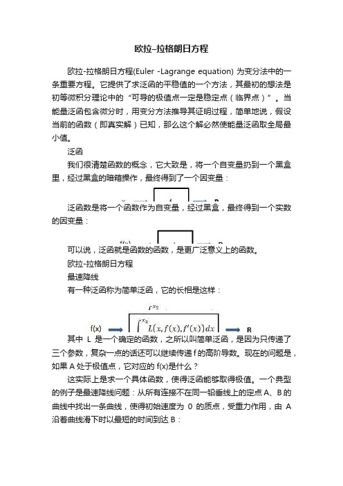
欧拉–拉格朗日方程欧拉-拉格朗日方程(Euler -Lagrange equation) 为变分法中的一条重要方程。

它提供了求泛函的平稳值的一个方法，其最初的想法是初等微积分理论中的“可导的极值点一定是稳定点（临界点）”。

当能量泛函包含微分时，用变分方法推导其证明过程，简单地说，假设当前的函数（即真实解）已知，那么这个解必然使能量泛函取全局最小值。

泛函我们很清楚函数的概念，它大致是，将一个自变量扔到一个黑盒里，经过黑盒的暗箱操作，最终得到了一个因变量：泛函数是将一个函数作为自变量，经过黑盒，最终得到一个实数的因变量：可以说，泛函就是函数的函数，是更广泛意义上的函数。

欧拉-拉格朗日方程最速降线有一种泛函称为简单泛函，它的长相是这样：其中L是一个确定的函数，之所以叫简单泛函，是因为只传递了三个参数，复杂一点的话还可以继续传递f的高阶导数。

现在的问题是，如果A处于极值点，它对应的f(x)是什么？这实际上是求一个具体函数，使得泛函能够取得极值。

一个典型的例子是最速降线问题：从所有连接不在同一铅垂线上的定点A、B的曲线中找出一条曲线，使得初始速度为0的质点，受重力作用，由A 沿着曲线滑下时以最短的时间到达B：这里我们将曲线看作路径f关于时间t的函数：ΔSi是在极短时间Δti内沿着曲线移动的微小弧长，此时的瞬时速度是ΔVi，距离=速度×时间：重力加速的推论，在t时间处的速度v2 = 2gh：质点从A点到B点的总时间：根据弧长公式，可以将dS化简，进一步写成把结论和简单泛函做个对比，可以看到二者形式相吻合：最右侧的式子并没有严格映射到L(x,f(x),f’(x))，因为在函数中并没有直接使用到参数t，这无所谓了，可以理解成虽然传递了参数t，但实际上t并没有起任何作用，就像y (x) = 1一样，无论传递任何x，最终结果都是1，但它仍然是一个y关于x的函数。

现在回到最初的问题，AB间有无数条曲线，每条曲线都可以求得时间T[f]，在众多的曲线中，有一条唯一的曲线能够使得T[f]取得最小值，这个f(x)应该长成什么样？EL方程的推导这里暂且耍一下流氓，抛开具体的速降问题，只看A[f]，并且假设f0(x)就是符合条件的最优函数。

欧拉（Euler）坐标系和拉格朗日（Lagrange）坐标系（转）

欧拉（Euler）坐标系和拉格朗⽇（Lagrange）坐标系
（转）
Euler坐标其坐标系本⾝是固定得，仅物体运动；
Lagrange坐标其坐标系是放在所描述得物体上随着物体⼀起运动得。

例如流体⼒学中拉格朗⽇坐标系，观察者位于⼀个流体单元上，并随流体⼀起运动。

欧拉坐标系，观察者位于空间的⼀个固定点，观察流过你所在的体积单元。

欧拉坐标是指空间坐标，如果对于质点运动来说，研究的是不同的质点经过空间⼀定点的状态
拉格朗⽇坐标指的是材料坐标，如果对于质点运动来说，是跟随着质点研究质点的运动状态
简单的说就是：欧拉坐标固定在空间，拉格朗⽇坐标固定在材料上
欧拉坐标指⼀点在空间的位置，拉格朗⽇坐标标记⼀个材料点
另：
研究流体流动的⽅法基本上有两种：
⼀种是类似与追踪法的⽅法，如研究空⽓流动状态时，将⼀⽚⽻⽑⼊流场中，⽻⽑的轨迹就显⽰了该点空⽓运动的状态；
另⼀种⽅法就是固定观察区域，不管流动怎么变化，研究的只是固定区域的流动状况。

好象后⾯⼀种就是拉格朗⽇法，前⾯的是欧拉法，不过⼀般研究流体运动都是⽤的拉格朗⽇法。

欧拉拉格朗日方程小时百科

欧拉拉格朗日方程小时百科欧拉-拉格朗日方程（Euler-Lagrange equation）是经典力学中的重要数学工具，在研究守恒定律和运动方程问题时具有广泛的应用。

它是由瑞士数学家欧拉和法国数学家拉格朗日相继发现的，因此得名。

欧拉-拉格朗日方程描述了系统在任意时刻的运动方程，可以从一个称为拉格朗日量（Lagrangian）的函数中导出。

拉格朗日量是系统的动能减势能的差，通常记为L=T-V，其中T表示动能，V表示势能。

欧拉-拉格朗日方程的一般形式可以表示为：∂(∂L/∂(q̇_i))/∂t-∂L/∂q_i=0其中，q_i代表广义坐标，q̇_i代表q_i对时间的导数，∂/∂t表示对时间的偏导数，∂/∂q_i表示对q_i的偏导数。

欧拉-拉格朗日方程可以推导出系统的运动方程，即确定系统在一系列广义坐标下的运动规律。

它是一种形式均不急剧的微分方程，可以通过一系列数学方法来解。

欧拉-拉格朗日方程的导出过程较为复杂，需要用到变分法和微积分工具。

简单来说，利用变分法可以将运动方程推广到任意变动路径上，将系统的动力学问题转化为优化问题，从而可以得到最优路径的运动方程。

欧拉-拉格朗日方程的重要性在于它能够描述物理系统的运动规律，并且很多物理理论可以从欧拉-拉格朗日方程导出。

尤其是在经典力学中，欧拉-拉格朗日方程可以成功解决多体系统的运动问题，是经典力学的基石之一。

除了经典力学，欧拉-拉格朗日方程还可以应用于其他物理学领域，如电动力学、量子场论、相对论等。

在这些领域中，拉格朗日量可以通过对系统的物理特性进行描述，从而得到欧拉-拉格朗日方程。

总之，欧拉-拉格朗日方程作为经典力学中的重要工具，具有广泛的应用价值。

它通过拉格朗日量的构造，描述了系统在各种广义坐标下的运动规律，为物理学研究提供了有力的数学工具。

正是由于欧拉-拉格朗日方程的存在，我们能够更好地理解和掌握物理世界的运动规律。

Euler与Lagrange观点下的连续方程

欧拉观点的连续方程：
微商符：可得：又已知(2.2) 带入（2.2）,并合并就得到：
（2.6）是欧拉观点的连续方程，也是我们常用的形式。）是欧拉观点的连续方程，也是我们常用的形式。
欧拉观点的连续方程
各项的物理意义：：流体密度的局地变化：单位体积的流体质量通量欧拉观点的连续方程的物理意义：欧拉观点的连续方程的物理意义：空间某点流体质量有净外流时( )，该点密度必然减少( ，该点密度必然减少 )，反之亦，
然。可见，流动改变了流体质量的分布。可见，流动改变了流体质量的分布。
讨论：
的流体称为【无辐散流体】，也称为【不可压缩流体】。此时根据(2.2) 可知：
拉氏观点欧氏观点
表示了密度的不均匀性。（若 ∇ ρ=0 表示密度在空间处处都一样）表示了流体的定常和非定常性。为定常；为非定常）
（
可见，流体质点在运动中保持密度不变）可见，当（流体质点在运动中保持密度不变）时，流体场内的流体密度可以不定常和不均匀，流体场内的流体密度可以不定常和不均匀，只要这两者的变化对流体块的贡献正好抵消就可以。变化对流体块的贡献正好抵消就可以。
Байду номын сангаас
特例：
【均质流体】流体密度空间处处相等，但可能随时间均质流体】在变化，只不过，不管怎么变化，密度处处相同，或说密度处处发生着相同的变化。
【不可压缩流体】某一流体质点在运不可压缩流体】动中保持密度不变。但个个空间上的密度可能不同。
【均匀不可压缩流体】密度不但在空间处处相等，而且在运动均匀不可压缩流体】中还保持不变。均匀不可压缩流体也可以叫做【定常不可压】。
这个流体团的体积是在运动中质量守恒，即：展开得到：

欧拉-拉格朗日方程

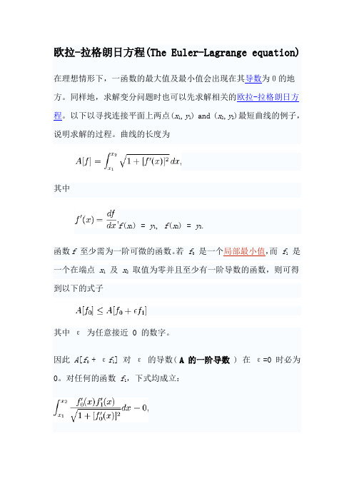
欧拉-拉格朗日方程(The Euler-Lagrange equation) 在理想情形下，一函数的最大值及最小值会出现在其导数为０的地方。

同样地，求解变分问题时也可以先求解相关的欧拉-拉格朗日方程。

以下以寻找连接平面上两点(x1,y1) and (x2,y2)最短曲线的例子，说明求解的过程。

曲线的长度为其中f(x1) = y1, f(x2) = y2.函数f至少需为一阶可微的函数。

若f0是一个局部最小值，而f1是一个在端点x1及x2取值为零并且至少有一阶导数的函数，则可得到以下的式子其中ε为任意接近 0 的数字。

因此A[f0+ εf1] 对ε的导数( A 的一阶导数 ) 在ε=0 时必为0。

对任何的函数f1，下式均成立：此条件可视为在可微分函数的空间中，A[f0] 在各方向的导数均为0。

若假设f0二阶可微(或至少弱微分存在)，则利用分部积分法可得其中f1为在两端点皆为 0 的任意二阶可微函数。

这是变分法基本引理的一个特例:其中f1为在两端点皆为 0 的任意可微函数。

若存在使H(x) > 0，则在周围有一区间的 H 也是正值。

可以选择f1在此区间外为 0，在此区间内为非负值，因此I > 0，和前提不合。

若存在使H(x) < 0，也可证得类似的结果。

因此可得到以下的结论：由结论可推得下式：因此两点间最短曲线为一直线。

在一般情形下，则需考虑以下的计算式其中f需有二阶连续的导函数。

在这种情形下，拉格朗日量L在极值f0处满足欧拉-拉格朗日方程不过在此处，欧拉-拉格朗日方程只是有极值的必要条件，并不是充分条件。

流体运动描述方法(欧拉法和拉格朗日法)

流体运动描述方法(欧拉法和拉格朗日法) -CAL-FENGHAI.-(YICAI)-Company One1在流体力学里，有两种描述流体运动的方法：欧拉（Euler)和拉格朗日（Lagrange)方法。

欧拉法描述的是任何时刻流场中各种变量的分布，而拉格朗日法却是去追踪每个粒子从某一时刻起的运动轨迹。

在一个风和日丽的午后，YC坐在河岸边看河水流，恩，她总是很闲。

如果YC 的位置不动，她在自己目光能及的河面上划出一块区域，数某一时刻经过的船只数，如果可能的话，再数数经过的鱼儿数；当然，如果手头有些仪器，她可以干干正事，比如测测水流的速度、水的压力、水的温度等，由此得到每一时刻这一河流区域水流各物理量的分布。

那么YC是在用欧拉方法研究流体。

这时，YC忽然看到一条船上坐着她的初恋情人，虽然根据陈安对初恋情人的定义，YC根本没有初恋情人。

现在假设她有，天哪，他们有20年没见面了，他还欠她20元呢，不能放了他。

于是YC记下第一眼看到初恋情人的时间，并迅速测出此时船的位置和速度，然后撒腿追去。

假设这条船是顺水而下，船的速度即是水流的速度。

每隔一个时间点，她便测一下船的速度和位置。

为了曾经的爱情，还有那不计利息的20元，她越过山岗，淌过小溪，直到那条船离开了她的视线。

于是，她得到了这条船在河流中的运动轨迹。

YC此时所用的研究方法就是拉格朗日法。

Understood而在一些复杂的两相流动问题里，比如粒子在流场中运动的问题，我们关注的是粒子的运动轨迹，因此，我们可以用拉格朗日方法追踪粒子在流场中的运动，同时，用欧拉方法来计算流场的各物理量。

在许多工程领域，都有纤维在流场中运动的问题。

如果将纤维在流场中的运动视为两相流动，必须为纤维作一些改变，因为它不同于一般的刚性粒子。

它细长，细长到你无法用一个粒子来代表一根纤维；它柔，柔得自己的每一部分可以相对于其他部分发生变形。

我在《柔性纤维的妖娆运动》里，为slender and flexible纤维建立了模型，把纤维离散成一个个粒子，并在粒子之间建立了弹性或粘弹性的连接。

拉格朗日方程

拉格朗日方程，因约瑟夫·路易斯·拉格朗日而命名，是拉格朗日力学的主要方程，可以用来描述物体的运动，特别适用于理论物理的研究。

拉格朗日方程的功能相等于牛顿力学中的牛顿第二定律。

简介
拉格朗日方程：对于完整系统用广义坐标表示的动力方程，通常系指第二类拉格朗日方程,是法国数学家J.-L.拉格朗日首先导出的。

应用
用拉格朗日方程解题的优点是：①广义坐标个数通常比x坐标少，即N<3n，故拉氏方程个数比直角坐标的牛顿方程个数少，即运动微分方程组的阶数较低，问题易于求解；②广义坐标可根据约束条件作适当的选择，使力学问题的运算简化，并且不必考虑约束力；③T和L都是标量，比力的矢量关系式更易表达，因此较易列出动力方程。

下面是两个例子：
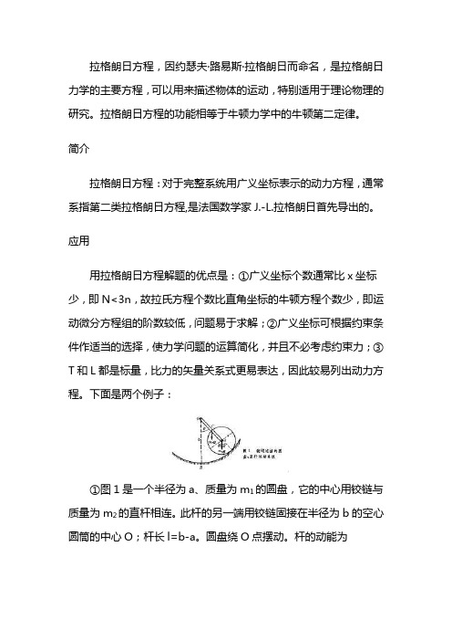
①图1是一个半径为a、质量为m1的圆盘，它的中心用铰链与质量为m2的直杆相连。

此杆的另一端用铰链固接在半径为b的空心圆筒的中心O；杆长l=b-a。

圆盘绕O点摆动。

杆的动能为
圆盘转动角关系为bθ=a(θ+φ)，圆盘绕O点转动动能为
系统以B点为标准的势能V和系统的动能T为：
代入。