H. DLV-HEX Dealing with Semantic Web under Answer-Set Programming
深度优先局部聚合哈希

Vol.48,No.6Jun. 202 1第48卷第6期2 0 2 1年6月湖南大学学报)自然科学版)Journal of Hunan University (Natural Sciences )文章编号:1674-2974(2021 )06-0058-09 DOI : 10.16339/ki.hdxbzkb.2021.06.009深度优先局艺B 聚合哈希龙显忠g,程成李云12(1.南京邮电大学计算机学院,江苏南京210023;2.江苏省大数据安全与智能处理重点实验室,江苏南京210023)摘 要:已有的深度监督哈希方法不能有效地利用提取到的卷积特征,同时,也忽视了数据对之间相似性信息分布对于哈希网络的作用,最终导致学到的哈希编码之间的区分性不足.为了解决该问题,提出了一种新颖的深度监督哈希方法,称之为深度优先局部聚合哈希(DeepPriority Local Aggregated Hashing , DPLAH ). DPLAH 将局部聚合描述子向量嵌入到哈希网络 中,提高网络对同类数据的表达能力,并且通过在数据对之间施加不同权重,从而减少相似性 信息分布倾斜对哈希网络的影响.利用Pytorch 深度框架进行DPLAH 实验,使用NetVLAD 层 对Resnet18网络模型输出的卷积特征进行聚合,将聚合得到的特征进行哈希编码学习.在CI-FAR-10和NUS-WIDE 数据集上的图像检索实验表明,与使用手工特征和卷积神经网络特征的非深度哈希学习算法的最好结果相比,DPLAH 的平均准确率均值要高出11%,同时,DPLAH 的平均准确率均值比非对称深度监督哈希方法高出2%.关键词:深度哈希学习;卷积神经网络;图像检索;局部聚合描述子向量中图分类号:TP391.4文献标志码:ADeep Priority Local Aggregated HashingLONG Xianzhong 1,覮,CHENG Cheng1,2,LI Yun 1,2(1. School of Computer Science & Technology ,Nanjing University of Posts and Telecommunications ,Nanjing 210023, China ;2. Key Laboratory of Jiangsu Big Data Security and Intelligent Processing ,Nanjing 210023, China )Abstract : The existing deep supervised hashing methods cannot effectively utilize the extracted convolution fea tures, but also ignore the role of the similarity information distribution between data pairs on the hash network, result ing in insufficient discrimination between the learned hash codes. In order to solve this problem, a novel deep super vised hashing method called deep priority locally aggregated hashing (DPLAH) is proposed in this paper, which em beds the vector of locally aggregated descriptors (VLAD) into the hash network, so as to improve the ability of the hashnetwork to express the similar data, and reduce the impact of similarity distribution skew on the hash network by im posing different weights on the data pairs. DPLAH experiment is carried out by using the Pytorch deep framework. Theconvolution features of the Resnet18 network model output are aggregated by using the NetVLAD layer, and the hashcoding is learned by using the aggregated features. The image retrieval experiments on the CIFAR-10 and NUS - WIDE datasets show that the mean average precision (MAP) of DPLAH is11 percentage points higher than that of* 收稿日期:2020-04-26基金项目:国家自然科学基金资助项目(61906098,61772284),National Natural Science Foundation of China(61906098, 61772284);国家重 点研发计划项目(2018YFB 1003702) , National Key Research and Development Program of China (2018YFB1003702)作者简介:龙显忠(1985—),男,河南信阳人,南京邮电大学讲师,工学博士,硕士生导师覮 通信联系人,E-mail : *************.cn第6期龙显忠等:深度优先局部聚合哈希59non-deep hash learning algorithms using manual features and convolution neural network features,and the MAP of DPLAH is2percentage points higher than that of asymmetric deep supervised hashing method.Key words:deep Hash learning;convolutional neural network;image retrieval;vector of locally aggregated de-scriptors(VLAD)随着信息检索技术的不断发展和完善,如今人们可以利用互联网轻易获取感兴趣的数据内容,然而,信息技术的发展同时导致了数据规模的迅猛增长.面对海量的数据以及超大规模的数据集,利用最近邻搜索[1(Nearest Neighbor Search,NN)的检索技术已经无法获得理想的检索效果与可接受的检索时间.因此,近年来,近似最近邻搜索[2(Approximate Nearest Neighbor Search,ANN)变得越来越流行,它通过搜索可能相似的几个数据而不再局限于返回最相似的数据,在牺牲可接受范围的精度下提高了检索效率.作为一种广泛使用的ANN搜索技术,哈希方法(Hashing)[3]将数据转换为紧凑的二进制编码(哈希编码)表示,同时保证相似的数据对生成相似的二进制编码.利用哈希编码来表示原始数据,显著减少了数据的存储和查询开销,从而可以应对大规模数据中的检索问题.因此,哈希方法吸引了越来越多学者的关注.当前哈希方法主要分为两类:数据独立的哈希方法和数据依赖的哈希方法,这两类哈希方法的区别在于哈希函数是否需要训练数据来定义.局部敏感哈希(Locality Sensitive Hashing,LSH)[4]作为数据独立的哈希代表,它利用独立于训练数据的随机投影作为哈希函数•相反,数据依赖哈希的哈希函数需要通过训练数据学习出来,因此,数据依赖的哈希也被称为哈希学习,数据依赖的哈希通常具有更好的性能.近年来,哈希方法的研究主要侧重于哈希学习方面.根据哈希学习过程中是否使用标签,哈希学习方法可以进一步分为:监督哈希学习和无监督哈希学习.典型的无监督哈希学习包括:谱哈希[5(Spectral Hashing,SH);迭代量化哈希[6](Iterative Quantization, ITQ);离散图哈希[7(Discrete Graph Hashing,DGH);有序嵌入哈希[8](Ordinal Embedding Hashing,OEH)等.无监督哈希学习方法仅使用无标签的数据来学习哈希函数,将输入的数据映射为哈希编码的形式.相反,监督哈希学习方法通过利用监督信息来学习哈希函数,由于利用了带有标签的数据,监督哈希方法往往比无监督哈希方法具有更好的准确性,本文的研究主要针对监督哈希学习方法.传统的监督哈希方法包括:核监督哈希[9](Supervised Hashing with Kernels,KSH);潜在因子哈希[10](Latent Factor Hashing,LFH);快速监督哈希[11](Fast Supervised Hashing,FastH);监督离散哈希[1(Super-vised Discrete Hashing,SDH)等.随着深度学习技术的发展[13],利用神经网络提取的特征已经逐渐替代手工特征,推动了深度监督哈希的进步.具有代表性的深度监督哈希方法包括:卷积神经网络哈希[1(Convolutional Neural Networks Hashing,CNNH);深度语义排序哈希[15](Deep Semantic Ranking Based Hash-ing,DSRH);深度成对监督哈希[16](Deep Pairwise-Supervised Hashing,DPSH);深度监督离散哈希[17](Deep Supervised Discrete Hashing,DSDH);深度优先哈希[18](Deep Priority Hashing,DPH)等.通过将特征学习和哈希编码学习(或哈希函数学习)集成到一个端到端网络中,深度监督哈希方法可以显著优于非深度监督哈希方法.到目前为止,大多数现有的深度哈希方法都采用对称策略来学习查询数据和数据集的哈希编码以及深度哈希函数.相反,非对称深度监督哈希[19](Asymmetric Deep Supervised Hashing,ADSH)以非对称的方式处理查询数据和整个数据库数据,解决了对称方式中训练开销较大的问题,仅仅通过查询数据就可以对神经网络进行训练来学习哈希函数,整个数据库的哈希编码可以通过优化直接得到.本文的模型同样利用了ADSH的非对称训练策略.然而,现有的非对称深度监督哈希方法并没有考虑到数据之间的相似性分布对于哈希网络的影响,可能导致结果是:容易在汉明空间中保持相似关系的数据对,往往会被训练得越来越好;相反,那些难以在汉明空间中保持相似关系的数据对,往往在训练后得到的提升并不显著.同时大部分现有的深度监督哈希方法在哈希网络中没有充分有效利用提60湖南大学学报(自然科学版)2021年取到的卷积特征.本文提出了一种新的深度监督哈希方法,称为深度优先局部聚合哈希(Deep Priority Local Aggregated Hashing,DPLAH).DPLAH的贡献主要有三个方面:1)DPLAH采用非对称的方式处理查询数据和数据库数据,同时DPLAH网络会优先学习查询数据和数据库数据之间困难的数据对,从而减轻相似性分布倾斜对哈希网络的影响.2)DPLAH设计了全新的深度哈希网络,具体来说,DPLAH将局部聚合表示融入到哈希网络中,提高了哈希网络对同类数据的表达能力.同时考虑到数据的局部聚合表示对于分类任务的有效性.3)在两个大型数据集上的实验结果表明,DPLAH在实际应用中性能优越.1相关工作本节分别对哈希学习[3]、NetVLAD[20]和Focal Loss[21]进行介绍.DPLAH分别利用NetVLAD和Focal Loss提高哈希网络对同类数据的表达能力及减轻数据之间相似性分布倾斜对于哈希网络的影响. 1.1哈希学习哈希学习[3]的任务是学习查询数据和数据库数据的哈希编码表示,同时要满足原始数据之间的近邻关系与数据哈希编码之间的近邻关系相一致的条件.具体来说,利用机器学习方法将所有数据映射成{0,1}r形式的二进制编码(r表示哈希编码长度),在原空间中不相似的数据点将被映射成不相似)即汉明距离较大)的两个二进制编码,而原空间中相似的两个数据点将被映射成相似(即汉明距离较小)的两个二进制编码.为了便于计算,大部分哈希方法学习{-1,1}r形式的哈希编码,这是因为{-1,1}r形式的哈希编码对之间的内积等于哈希编码的长度减去汉明距离的两倍,同时{-1,1}r形式的哈希编码可以容易转化为{0,1}r形式的二进制编码.图1是哈希学习的示意图.经过特征提取后的高维向量被用来表示原始图像,哈希函数h将每张图像映射成8bits的哈希编码,使原来相似的数据对(图中老虎1和老虎2)之间的哈希编码汉明距离尽可能小,原来不相似的数据对(图中大象和老虎1)之间的哈希编码汉明距离尽可能大.h(大象)=10001010h(老虎1)=01100001h(老虎2)=01100101相似度尽可能小相似度尽可能大图1哈希学习示意图Fig.1Hashing learning diagram1.2NetVLADNetVLAD的提出是用于解决端到端的场景识别问题[20(场景识别被当作一个实例检索任务),它将传统的局部聚合描述子向量(Vector of Locally Aggregated Descriptors,VLAD[22])结构嵌入到CNN网络中,得到了一个新的VLAD层.可以容易地将NetVLAD 使用在任意CNN结构中,利用反向传播算法进行优化,它能够有效地提高对同类别图像的表达能力,并提高分类的性能.NetVLAD的编码步骤为:利用卷积神经网络提取图像的卷积特征;利用NetVLAD层对卷积特征进行聚合操作.图2为NetVLAD层的示意图.在特征提取阶段,NetVLAD会在最后一个卷积层上裁剪卷积特征,并将其视为密集的描述符提取器,最后一个卷积层的输出是H伊W伊D映射,可以将其视为在H伊W空间位置提取的一组D维特征,该方法在实例检索和纹理识别任务[23別中都表现出了很好的效果.NetVLAD layer(KxD)x lVLADvectorh------->图2NetVLAD层示意图⑷Fig.2NetVLAD layer diagram1201NetVLAD在特征聚合阶段,利用一个新的池化层对裁剪的CNN特征进行聚合,这个新的池化层被称为NetVLAD层.NetVLAD的聚合操作公式如下:NV((,k)二移a(x)(血⑺-C((j))(1)i=1式中:血(j)和C)(j)分别表示第i个特征的第j维和第k个聚类中心的第j维;恣&)表示特征您与第k个视觉单词之间的权.NetVLAD特征聚合的输入为:NetVLAD裁剪得到的N个D维的卷积特征,K个聚第6期龙显忠等:深度优先局部聚合哈希61类中心.VLAD的特征分配方式是硬分配,即每个特征只和对应的最近邻聚类中心相关联,这种分配方式会造成较大的量化误差,并且,这种分配方式嵌入到卷积神经网络中无法进行反向传播更新参数.因此,NetVLAD采用软分配的方式进行特征分配,软分配对应的公式如下:-琢II Xi-C*II 2=—e(2)-琢II X-Ck,II2k,如果琢寅+肄,那么对于最接近的聚类中心,龟&)的值为1,其他为0.aS)可以进一步重写为:w j X i+b ka(x i)=—e-)3)w J'X i+b kk,式中:W k=2琢C k;b k=-琢||C k||2.最终的NetVLAD的聚合表示可以写为:N w;x+b kv(j,k)=移—----(x(j)-Ck(j))(4)i=1w j.X i+b k移ek,1.3Focal Loss对于目标检测方法,一般可以分为两种类型:单阶段目标检测和两阶段目标检测,通常情况下,两阶段的目标检测效果要优于单阶段的目标检测.Lin等人[21]揭示了前景和背景的极度不平衡导致了单阶段目标检测的效果无法令人满意,具体而言,容易被分类的背景虽然对应的损失很低,但由于图像中背景的比重很大,对于损失依旧有很大的贡献,从而导致收敛到不够好的一个结果.Lin等人[21]提出了Focal Loss应对这一问题,图3是对应的示意图.使用交叉爛作为目标检测中的分类损失,对于易分类的样本,它的损失虽然很低,但数据的不平衡导致大量易分类的损失之和压倒了难分类的样本损失,最终难分类的样本不能在神经网络中得到有效的训练.Focal Loss的本质是一种加权思想,权重可根据分类正确的概率p得到,利用酌可以对该权重的强度进行调整.针对非对称深度哈希方法,希望难以在汉明空间中保持相似关系的数据对优先训练,具体来说,对于DPLAH的整体训练损失,通过施加权重的方式,相对提高难以在汉明空间中保持相似关系的数据对之间的训练损失.然而深度哈希学习并不是一个分类任务,因此无法像Focal Loss一样根据分类正确的概率设计权重,哈希学习的目的是学到保相似性的哈希编码,本文最终利用数据对哈希编码的相似度作为权重的设计依据具体的权重形式将在模型部分详细介绍.正确分类的概率图3Focal Loss示意图[21】Fig.3Focal Loss diagram12112深度优先局部聚合哈希2.1基本定义DPLAH模型采用非对称的网络设计.Q={0},=1表示n张查询图像,X={X i}m1表示数据库有m张图像;查询图像和数据库图像的标签分别用Z={Z i},=1和Y ={川1表示;i=[Z i1,…,zj1,i=1,…,n;c表示类另数;如果查询图像0属于类别j,j=1,…,c;那么z”=1,否则=0.利用标签信息,可以构造图像对的相似性矩阵S沂{-1,1}"伊”,s”=1表示查询图像q,和数据库中的图像X j语义相似,S j=-1表示查询图像和数据库中的图像X j语义不相似.深度哈希方法的目标是学习查询图像和数据库中图像的哈希编码,查询图像的哈希编码用U沂{-1,1}"",表示,数据库中图像的哈希编码用B沂{-1,1}m伊r表示,其中r表示哈希编码的长度.对于DPLAH模型,它在特征提取部分采用预训练好的Resnet18网络[25].图4为DPLAH网络的结构示意图,利用NetVLAD层聚合Resnet18网络提取到的卷积特征,哈希编码通过VLAD编码得到,由于VLAD编码在分类任务中被广泛使用,于是本文将NetVLAD层的输出作为分类任务的输入,利用图像的标签信息监督NetVLAD层对卷积特征的利用.事实上,任何一种CNN模型都能实现图像特征提取的功能,所以对于选用哪种网络进行特征学习并不是本文的重点.62湖南大学学报(自然科学版)2021年conv1图4DPLAH结构Fig.4DPLAH structure图像标签soft-max1,0,1,1,0□1,0,0,0,11,1,0,1,0---------*----------VLADVLAD core)c)l・>:i>数据库图像的哈希编码2.2DPLAH模型的目标函数为了学习可以保留查询图像与数据库图像之间相似性的哈希编码,一种常见的方法是利用相似性的监督信息S e{-1,1}n伊"、生成的哈希编码长度r,以及查询图像的哈希编码仏和数据库中图像的哈希编码b三者之间的关系[9],即最小化相似性的监督信息与哈希编码对内积之间的L损失.考虑到相似性分布的倾斜问题,本文通过施加权重来调节查询图像和数据库图像之间的损失,其公式可以表示为:min J=移移(1-w)(u T b j-rs)专,B i=1j=1s.t.U沂{-1,1}n伊r,B沂{-1,1}m伊r,W沂R n伊m(5)受FocalLoss启发,希望深度哈希网络优先训练相似性不容易保留图像对,然而Focal Loss利用图像的分类结果对损失进行调整,因此,需要重新进行设计,由于哈希学习的目的是为了保留图像在汉明空间中的相似性关系,本文利用哈希编码的余弦相似度来设计权重,其表达式为:1+。
基于强化学习的实体关系联合抽取模型

2019-07-10http://www. joca. cnJournal of Computer Applications 计算机应用,2019,39(7):1918 -1924ISSN 1001-9081CODEN JYIIDU文章编号:1001-9081 (2019)07-1918-07DOI : 10.11772/j. issn. 1001-9081.2019010182基于强化学习的实体关系联合抽取模型陈佳洋,滕冲(武汉大学国家网络安全学院,武汉430072)(*通信作者电子邮箱tengchong@ whu. edu. cn)摘 要:针对现有的基于远程监督的实体和关系抽取方法存在着标签噪声问题,提出了一种基于强化学习的实 体关系联合抽取方法。
该模型有两个模块:句子选择器模块和实体关系联合抽取模块。
首先,句子选择器模块选择没有标签噪声的高质量句子,将所选句子输入到实体关系联合抽取模型;然后,实体关系联合抽取模块采用序列标注方法对输入的句子进行预测,并向句子选择器模块提供反馈,指导句子选择器模块挑选高质量的句子;最后,句子选择 器模块和实体关系联合抽取模块同时训练,将句子选择与序列标注一起优化。
实验结果表明,该模型在实体关系联合抽取中的F1值为47.3%,与CoType 为代表的联合抽取模型相比,所提模型的F1值提升了 1% ;与LINE 为代表的串行模型相比,所提模型的F1值提升了 14%。
结果表明强化学习结合实体关系联合抽取模型能够有效地提高序列标注模型的F1值,其中句子选择器能有效地处理数据的噪声。
关键词:强化学习;联合抽取;序列标注;命名实体识别;关系分类中图分类号:TP389.1 文献标志码:AJoint entity and relation extraction model based on reinforcement learningCHEN Jiafeng, TENG Chong *(School of Cyber Science and Engineering, Wuhan University, Wuhan Hubei 430072, China)Abstract : Existing entity and relation extraction methods that rely on distant supervision suffer from noisy labelingproblem. A model for joint entity and relation extraction from noisy data based on reinforcement learning was proposed toreduce the impact o£ noise data. There were two modules in the model: an sentence selector module and a sequence labeling module. Firstly, high-quality sentences without labeling noise were selected by instance selector module and the selectedsentences were input into sequence labeling module. Secondly, predictions were made by sequence labeling module and therewards were provided to sentence selector module to help the module select high-quality sentences. Finally, two modules weretrained jointly to optimize instance selection and sequence labeling processes. The experimental results show that the Fl value o£ the proposed model is 47. 3% in the joint entity and relation extraction, which is 1% higher than those o£ joint extraction models represented by CoType and 14% higher than those o£ serial models represented by LINE ( Large-scale InformationNetwork Embedding). The results show that the joint entity and relation extraction model in combination with reinforcementlearning can eflectively improve Fl value of sequential labeling model, in which the sentence selector can effectively deal withthe noise o£ data.Key words : reinforcement learning; joint extraction; sequence tagging; named entity recognition; relation classification0引言实体和关系的联合抽取是从非结构化文本中同时检测实体引用和识别它们的语义关系,如图1所示。
stable diffusion wenui 原理

Stable Diffusion是一种潜在扩散模型(LDM),它可以从文本描述生成高质量的图像。
其工作原理可以总结为以下步骤:
1. Stable Diffusion由变分自编码器(V AE)、U-Net和一个可选的文本编码器组成。
2. V AE编码器将图像从像素空间压缩到一个更小维度的潜在空间,捕捉图像的更本质的语义含义。
3. U-Net是一个卷积神经网络,它可以从潜在空间重建图像,并去除高斯噪声。
4. 文本编码器是一个预训练的模型,它可以将文本描述转换为一个向量,用来指导图像生成的过程。
5. Stable Diffusion的生成过程是一个迭代的去噪过程。
它从一个随机噪声开始,然后逐步减少噪声的强度,同时根据文本编码器的输出调整图像的内容,直到达到预设的步数为止,最终得到想要的图像。
希望以上信息对你有帮助。
云计算第三版Amazon云计算AWS

3.1 基础存储架构Dynamo
《云计算》第三版配套PPT课件
成员资格及错误检测
为了避免新加入的节点之间不能及时发现其他节点的存在,Dynamo中设置了一些 种子节点(Seed Node)。种子节点和所有的节点都有联系。当新节点加入时, 它扮演一个中介的角色,使新加入节点之间互相感知。
新节点 1
新节点 2
直到N个节点全部传遍
结论:
Dynamo中的节点数不能太多 Amazon采用了分层Dynamo结构 来解决该问题
25 of 52
容错机制 《云计算》第三版配套PPT课件
由于成本方面的原因,Dynamo中很多服务器采用的是普通 PC主机; 其硬盘性能和专业服务器硬盘相差很远,出错很难避免; Dynamo中容错机制非常重要
11 of 52
《云计算》第三版配套PPT课件
数据均衡《云分计算布》第的三版问配套P题PT课件
➢一致性哈希算法
平衡性 单调性 分散性 负载
两步进行:
求出设备节点的哈希值,并
配置到环上的一个点;接着
计算数据的哈希值,按顺时
针方向将其存放到环上第一
个大于或等于数据哈希值的
节点上; 添加新节点时,按
照上述规则,调整相关数据
问题 数据均衡分布
数据备份 数据冲突处理 成员资格及错误检测 临时故障处理 永久故障处理
采取的相关技术 改进的一致性哈希算法 参数可调的弱quorum机制 向量时钟(Vector Clock) 基于Gossip协议的成员资格和错误检测 Hinted handoff(数据回传机制),
Merkle哈希树
种子节点
A B
C
24 of 52
3.1 基础存储架构Dynamo
快速最近邻矢量量化码字搜索算法

快速最近邻矢量量化码字搜索算法
孙圣和;陆哲明;刘春和
【期刊名称】《电子学报》
【年(卷),期】2001(029)0z1
【摘要】本文综述了各种快速最近邻矢量量化码字搜索算法,按照算法的特点对各种快速算法进行了归类,对各种算法的编码时间、平均失真计算次数、额外存储量和离线计算量进行了仿真、比较和分析,并提出作者的一些改进算法或改进思路.【总页数】6页(P1772-1777)
【作者】孙圣和;陆哲明;刘春和
【作者单位】哈尔滨工业大学自动化测试与控制系,黑龙江哈尔滨,150001;哈尔滨工业大学自动化测试与控制系,黑龙江哈尔滨,150001;哈尔滨工业大学自动化测试与控制系,黑龙江哈尔滨,150001
【正文语种】中文
【中图分类】TN919.31
【相关文献】
1.基于子矢量技术的矢量量化码字快速搜索算法 [J], 陈善学;徐皓淋
2.一种基于不等式的矢量量化快速码字搜索算法 [J], 木春梅;韩守梅
3.哈德码变换域等均值等方差最近邻矢量量化码字搜索算法 [J], 姜守达;陆哲明;裴慧
4.等均值等范数最近邻矢量量化码字搜索算法 [J], 刘春和;陆哲明;孙圣和
5.等和值块扩展最近邻矢量量化码字搜索算法 [J], 王冬芳;余宁梅;张如亮;杨媛
因版权原因,仅展示原文概要,查看原文内容请购买。
用于生物分子网络比对的自适应匈牙利贪心混合算法的并行化

C 0DE N J YI I DU
h t t p : / / w w w . j o c a . a n
d o i : 1 0 . 1 1 7 7 2 / j . i s s n . 1 0 0 1 — 9 0 8 1 . 2 0 1 3 . 1 2 . 3 3 2 1
用 于生 物分 子 网络 比对 的 自适 应匈 牙 利贪 心混 合算 法 的并行 化
J o u r n a l o f C o mp u t e r Ap p l i c a t i o n s
I S SN 1 001 — 9 081
2 01 3— 1 2— 01
计算机应 用, 2 0 1 3 , 3 3 ( 1 2 ) : 3 3 2 1 — 3 3 2 5 文章编 号 : 1 0 0 1 — 9 0 8 1 ( 2 0 1 3 ) 1 2 ・ 3 3 2 1 — 0 5
Ab s t r a c t :B i o mo l e e u l a r n e t w o r k s a l i g n me n t i s a n i mp o r t a n t ie f l d ,a n d i t i s a n e f f e c t i v e w a y t o s t u d y b i o mo l e c u l a r
p h e n o m e n o n .A d a p t i v e Hu n g a r y G r e e d y A l g o i r t h m( A HG A)i s o n e o f t h e v a l i d b i o m o l e c u l a r n e t w o r k s li a g n m e n t a l g o i r t h m s .
纹理物体缺陷的视觉检测算法研究--优秀毕业论文

摘 要
在竞争激烈的工业自动化生产过程中,机器视觉对产品质量的把关起着举足 轻重的作用,机器视觉在缺陷检测技术方面的应用也逐渐普遍起来。与常规的检 测技术相比,自动化的视觉检测系统更加经济、快捷、高效与 安全。纹理物体在 工业生产中广泛存在,像用于半导体装配和封装底板和发光二极管,现代 化电子 系统中的印制电路板,以及纺织行业中的布匹和织物等都可认为是含有纹理特征 的物体。本论文主要致力于纹理物体的缺陷检测技术研究,为纹理物体的自动化 检测提供高效而可靠的检测算法。 纹理是描述图像内容的重要特征,纹理分析也已经被成功的应用与纹理分割 和纹理分类当中。本研究提出了一种基于纹理分析技术和参考比较方式的缺陷检 测算法。这种算法能容忍物体变形引起的图像配准误差,对纹理的影响也具有鲁 棒性。本算法旨在为检测出的缺陷区域提供丰富而重要的物理意义,如缺陷区域 的大小、形状、亮度对比度及空间分布等。同时,在参考图像可行的情况下,本 算法可用于同质纹理物体和非同质纹理物体的检测,对非纹理物体 的检测也可取 得不错的效果。 在整个检测过程中,我们采用了可调控金字塔的纹理分析和重构技术。与传 统的小波纹理分析技术不同,我们在小波域中加入处理物体变形和纹理影响的容 忍度控制算法,来实现容忍物体变形和对纹理影响鲁棒的目的。最后可调控金字 塔的重构保证了缺陷区域物理意义恢复的准确性。实验阶段,我们检测了一系列 具有实际应用价值的图像。实验结果表明 本文提出的纹理物体缺陷检测算法具有 高效性和易于实现性。 关键字: 缺陷检测;纹理;物体变形;可调控金字塔;重构
Keywords: defect detection, texture, object distortion, steerable pyramid, reconstruction
II
一种基于双哈希二叉树的中文分词词典机制
( 鞍 山师范学院高职院 辽宁 鞍 山 1 1 4 0 1 6 )
摘 要
汉语 自动分词是汉语信 息处理 的前提 , 词典是汉语 自动分 词的基础 , 分词 词典机制 的优 劣直接 影响到 中文分 词 的速 度
和效率。详细介绍汉语 自动分词 的三种方法及五种词典机 制, 提 出一种简洁 而有效 的中文分词 词典机制 , 并通过理论分 析和实验 对
Ab s t r a c t Au t o ma t i c Ch i n e s e wo r d s e g me n t a t i o n i s t h e p r e r e q u i s i t e f o r C h i n e s e i n f o r ma t i o n p r o c e s s i n g ,a n d d i c t i o n a r y i s t h e b a s i s o f
me c h a n i s ms a r e i n t r o d u c e d i n d e t a i l .I n t h e e n d,a s i mp l e a n d e f f e c t i v e d i c t i o n a y r me c h a n i s m f o r C h i n e s e w o r d s e g me n t a t i o n i s p r o p o s e d .
第3 0卷 第 5期
2 0 1 3年 5 月
计 算机 应 用与软件
Co mp u t e r App l i c a t i o n s a n d S o t f wa r e
V0 1 . 3 0 No. 5 Ma y 2 01 3
基于小波神经网络的数字信号调制方式识别
基于小波神经网络的数字信号调制方式识别梁晔;郝洁;石蕊【摘要】In view of the problem that the recognition method of digital signal modulation mode was easy to be affected by noise and the recognition error was large,we designed a recognition method of digital signal modulation mode based on wavelet neural network.Firstly,we collected digital signal and extracted the modulation recognition feature from the signal as the classification basis of the digital signal modulation mode.Secondly,we established classifier of digital signals modulation recognition based on neural network,and selected particle swarm optimization algorithm to determine the parameters of the neural network,so as to realize the digital signal modulation recognition. Finally,the simulation test of digital signals modulation recognition was realized on MATLAB 2016 platform.The test results show that,even if the signal-to-noise ratio of digital signal is low,the wavelet neural network can still obtain the ideal digital signal modulation recognition results,and the digital signal modulation recognition rate is higher than that of the contrast method,thus improving the performance of digital signal modulation recognition.%针对当前数字信号调制方式识别方法易受噪声影响、识别误差较大等问题,设计一种基于小波神经网络的数字信号调制方式识别方法.首先采集数字信号,并从信号中提取调制识别特征,作为数字信号调制方式分类依据;然后采用小波神经网络建立数字信号调制方式识别的分类器,并选择粒子群优化算法确定神经网络的参数,实现数字信号调制方式识别;最后在MATLAB 2016平台上实现数字信号调制方式识别的仿真测试.测试结果表明,即使数字信号的信噪比较低时,小波神经网络仍可获得较理想的数字信号调制方式识别结果,且数字信号调制方式识别率高于对比方法,从而提高了数字信号调制方式识别性能.【期刊名称】《吉林大学学报(理学版)》【年(卷),期】2018(056)002【总页数】7页(P382-388)【关键词】数字信号;调制方式;识别方法;神经网络;粒子群优化算法;分类器设计【作者】梁晔;郝洁;石蕊【作者单位】兰州城市学院电子与信息工程学院,兰州730070;西北民族大学电气工程学院,兰州730030;兰州城市学院电子与信息工程学院,兰州730070【正文语种】中文【中图分类】TP391.9在数字信号应用过程中, 信号的调制解调技术十分关键, 在数字信号进行解调时, 首先要知道数字信号的调制方式, 因此数字信号调制方式自动、快速准确识别的研究受到广泛关注[1-6].数字信号调制方式的识别最初采用人工方式实现, 首先通过具有相关知识的专业人员设置不同类型的解调器, 然后对接收到的数字信号进行变频处理, 将变频后的信号输入到解调器中, 最后结合自己的知识、波形以及声音得到数字信号调制方式. 该方法由于需要人工参与, 自动化程度低, 同时数字信号调制方式识别结果与专业人员自身知识密切相关, 导致数字信号调制方式识别正确率较低, 而且数字信号调制方式识别时间长, 无法满足数字信号发展的要求[7-8]. 随着数字信号和信息处理技术的不断完善, 目前已有许多新的数字信号调制方式自动识别方法, 如: 基于混沌理论的数字信号调制方式识别方法, 对数字信号进行混沌分析, 通过模式识别技术实现数字信号调制方式识别;基于星座图的数字信号调制方式识别方法;基于小波分析的数字信号调制方式识别方法; 基于高阶累积量的数字信号调制方式识别方法等. 这些方法在数字信号的信噪比较高时, 可获得较理想的数字信号调制方式识别结果[9-11], 但当信噪比减小时, 数字信号调制方式识别正确率急剧下降[12-13]. 文献[14-16]提出了基于BP神经网络的数字信号调制方式识别方法, 由于BP神经网络属于智能学习算法, 可对数字信号调制方式进行自动分类, 提高了数字信号调制方式的识别正确率, 但BP神经网络自身存在易陷入局部极小值等缺陷, 会对数字信号调制方式识别产生不利影响. 小波神经网络是小波理论和神经网络相结合的产物, 比其他神经网络具有更优的自组织、自学习和容错能力, 为数字信号调制方式识别的建模提供了一种新工具.针对目前数字信号调制方式识别方法存在正确率低等缺陷, 本文提出一种基于小波神经网络的数字信号调制方式识别方法. 首先从数字信号中提取调制方式识别的特征, 然后采用小波神经网络建立数字信号调制方式识别的分类器, 最后在MATLAB2016平台上实现数字信号调制方式识别的仿真测试. 实验结果验证了小波神经网络数字信号调制方式识别的有效性和优越性.1 小波神经网络的数字信号调制方式识别流程图1 数字信号调制方式的识别流程Fig.1 Identification process of digital signal modulation mode基于小波神经网络的数字信号调制方式识别方法工作流程可分为如下3个阶段:1) 采集数字信号, 并对信号进行预处理, 主要为信号的消噪处理;2) 提取数字信号调制方式识别的特征参数;3) 设计数字信号调制方式识别的分类器.基于小波神经网络的数字信号调制方式识别流程如图1所示.2 基于小波神经网络的数字信号调制方式识别方法设计2.1 数字信号的预处理设包含有噪声的数字信号为x(t)=s(t)+n(t), 其中s(t)和n(t)分别表示原始信号和噪声, 对x(t)进行变换可得wx(j,k)=ws(j,k)+wn(j,k), j=0,1,…,J; k=0,1,…,N,(1)其中: wm(j,k)(m=x,s,n)表示第j层上的不同信号变换系数; J表示分解层数; N 表示信号大小.由于n(t)的变换系数为wn(j,k), 因此数字信号去噪基本原理为:如果wn(j,k)小于某个固定值, 则表示其为噪声, 可以将其舍去;当wn(j,k)大于某个固定值时, 表示其为有用信号, 应该保留. 设去噪后的信号为本文选择软阈值进行去噪, 软阈值去噪函数定义为(2)其中sgn( )表示符号函数.2.2 提取数字信号的特征参数目前数字信号调制方式识别特征参数较多, 由于信号瞬时信息可更好描述数字信号调制方式的类型, 因此提取信号瞬时信息的6个特征参数:1) 数字信号幅度的标准差和均值分别为σa和u a, Rσa为两者的比值, 计算公式为(3)2) 数字信号的相位标准差和均值分别为σp和up, 其比值为Rσp, 计算公式为(4)3) A表示数字信号的零中心归一化瞬时幅度, 平均值M2的计算公式为(5)4) Af表示数字信号的零中心归一化瞬时频率,其中, af表示信号的瞬时频率; 均值MF1计算公式为(6)5) Af的归一化值为的均值MF2计算公式为(7)6) Af的相位为Ap, 均值MP1计算公式为(8)2.3 粒子群优化小波神经网络2.3.1 粒子群优化算法设粒子的位置和速度分别为Xi和Vi, 在解空间中, 粒子的位置更新通过不断跟踪自身最优解Pbest=(pi1,pi2,…,piD)和群体最优解Gbest=(pg1,pg2,…,pgD)实现, 计算公式为Vid=ω×Vid+c1×rand( )×(Pbest-xid)+c2×rand( )×(Gbest-xid),(9)Xid=Xid+Vid,(10)图2 小波神经网络结构Fig.2 Structure of wavelet neural network其中: rand( )表示随机数; d表示维数; c1和c2表示加速系数;ω表示权值.2.3.2 小波神经网络本文采用小波基函数代替隐含层激活函数产生小波神经网络, 通过小波神经网络对数字信号调制方式进行学习, 建立数字信号调制方式的分类器, 数字信号调制方式识别的小波神经网络结构如图2所示.小波函数可定义为(11)小波神经网络的隐含层第j个神经元的输入和输出分别为(12)其中:ωij表示输入层与隐含层间的连接权值;θj(k)表示隐含层的阈值. 小波神经网络的输出层第j个神经元的输入和输出分别为(14)(15)其中:ωjl表示隐含层与输出层间的连接权值;表示输出层的阈值. 通常情况下, 小波神经网络的激励函数定义为(16)小波神经网络的数字信号调制方式识别步骤如下:1) 采集数字信号, 并通过阈值法去除数字信号中的噪声;2) 从去除噪声的数字信号中提取信号瞬时信息的6个特征参数, 并做归一化处理(17)3) 根据信号瞬时信息的6个特征参数确定小波神经网络的拓扑结构, 并初始化小波神经网络相关参数;4) 确定粒子群的适应度函数, 将数字信号调制方式识别平均误差作为粒子群优化小波神经网络参数的适应函数值, 公式为(18)其中: di和tk分别表示数字信号调制方式识别类型和实际的数字信号调制方式; m 表示小波神经网络的输出节点数量; n表示数字信号调制方式的训练样本数量;5) 将数字信号调制方式识别的训练样本输入到小波神经网络进行学习, 并通过粒子群优化算法优化小波神经网络的权值和阈值;6) 根据新的粒子群适应度值对当前数字信号调制方式识别分类器参数最优解进行不断更新;7) 当找到数字信号调制方式识别分类器参数的最优解时, 粒子群算法寻优结束;8) 小波神经网络根据最优权值和阈值对数字信号调制方式识别的训练样本进行重新学习, 建立最优的数字信号调制方式识别分类器;9) 将待测试的数字信号调制方式识别样本输入到分类器中进行学习, 并输出该数字信号调制方式的类型.3 仿真测试3.1 测试环境为了分析小波神经网络的数字信号调制方式识别效果, 选择常用的7种数字调制信号作为测试对象, 仿真测试平台为MATLAB2016. 实验仿真参数设置如下: 载频为150 kHz, 采样频率为1 200 kHz, 码元速率为12 500 b/s, 采样点数为10 000; 神经网络输入层节点数为6, 神经网络的隐含层节点数为13, 神经网络输出层节点数为7; 粒子群优化算法迭代次数为100, 粒子群优化算法的粒子数为20, 粒子群优化算法的权值为0.95.3.2 结果与分析在数字信号的信噪比分别为0和20 dB条件下, 对7种不同类型的数字信号调制方式识别, 每种信号采集的样本数量均为20, 其中15个样本数量作为训练样本集, 用于建立数字信号调制方式识别的分类器, 剩余5个样本作为测试样本集, 采用基本小波神经网络和粒子群优化算法优化小波神经网络对样本进行学习和测试, 统计数字信号调制方式识别的最优目标函数值, 得到了基本小波神经网络和粒子群优化算法优化神经网络最优解对应的目标函数值变化曲线如图3所示. 由图3可见, 无论数字信号的信噪比为0或20 dB, 粒子群优化算法优化小波神经网络的最优适应度值均优于小波神经网络, 且加快了找到最优适应度值的速度, 表明采用粒子群优化算法搜索小波神经网络的连接权值和阈值可改善小波神经网络的性能.图3 不同信噪比条件下的适应度值变化曲线Fig.3 Change curves of fitness value under different signal-to-noise ratios当数字信号的信噪比为0~ 20 dB时, 采用本文数字信号调制方式识别方法对7种信号进行分类识别, 每种数字信号调制方式识别率列于表1. 由表1可见, 数字信号的信噪比越高, 数字信号调制方式识别率越高, 表明本文对原始数字信号进行去噪可获得高质量的数字信号, 能改善数字信号调制方式识别结果, 同时对于所有数字信号调制方式, 本文方法的平均识别均达90%以上, 识别率可满足数字信号处理应用85%的要求, 说明本文的数字信号调制方式识别方法是一种有效的、结果可靠的识别方法.表1 不同信噪比下的数字信号调制方式识别率(%)Table 1 Recognition rate (%)of digital signal modulation mode under different signal-to-noise ratios数字信号调制方式信噪比/dB051015202ASK91.1892.5896.4398.371004ASK89.4992.5995.3 396.3998.392FSK93.7291.4996.4597.211004FSK95.0593.8597.0197.9498.752PSK90.8093.4395.6098.101004PSK88.6893.6996.5396.5510016QAM91.8694.6896.6298.8998.95平均值91.5493.1996.2897.6499.44为表明本文提出的数字信号调制方式识别方法的优越性, 选择文献[17-18]中经典数字信号调制方式识别方法进行对比测试, 在相同的实验环境下, 数字信号的信噪比为0~ 20 dB时, 所有方法均进行10次独立的仿真实验, 统计其数字信号调制方式平均识别率和平均识别时间, 对比实验结果如图4所示.图4 与经典数字信号调制方式识别方法的性能对比Fig.4 Performance comparisons with classical methods of digital signal modulation recognition methods由图4可见:1) 在相同数字信号信噪比的条件下, 本文方法的数字信号调制方式平均识别率均高于文献[17]和文献[18]的数字信号调制方式识别方法, 这是由于本文算法通过小波神经网络建立了性能较优的数字信号调制方式识别分类器, 克服了当前数字信号调制方式识别方法错误率大、对噪声鲁棒性差等缺陷, 同时通过粒子群优化算法对小波神经网络的连接权值和阈值进行在线优化, 明显减少了数字信号调制方式识别误差, 提高了数字信号调制方式识别率;2) 在相同实验环境下, 本文方法的数字信号调制方式平均识别时间明显减少, 这是因为本文方法对原始数字信号进行了去噪处理, 抑制了噪声对数字信号调制方式建模的干扰, 提取了更优的数字信号调制方式识别特征, 简化了数字信号调制方式识别的分类器结果, 加快了数字信号调制方式识别速度, 具有更好的实用性.综上所述, 为了提高数字信号调制方式的识别和分类性能, 本文提出了一种基于神经网络的数字信号调制方式识别方法, 首先提取数字信号的瞬时特征, 并进行归一化处理作为神经网络的输入向量; 然后通过粒子群优化神经网络构建数字信号调制方式识别的分类器; 最后通过仿真测试结果表明, 无论是数字信号的信噪比高或低, 本文方法均可获得较理想的数字信号调制方式识别结果, 具有较强的抗噪性能.参考文献【相关文献】[1] Dobre O, Abid A, Bar-Ness Y, et al. Survey of Automatic Modulation Classification Techniques: Classical Approaches and New Trends [J]. IET Communieations, 2007, 21(2): 137-156.[2] WANG Jianghong, LI Bingbing, LIU Mingqian, et al. SNR Estimation of Time-Frequency Overlapped Signals for Underlay Cognitive Radio [J]. IEEE Communications Letters, 2015, 19(11): 1925-1928.[3] 徐闻, 王斌. 采用高阶累计量的时频混叠信号调制识别研究 [J]. 信息工程大学学报, 2013, 14(3): 299-305. (XU Wen, WANG Bin. Method of Modulation Recognition of Time-Frequency Overlapped Signals Based on High-Order Cumulants [J]. Journal of Information Engineering University, 2013, 14(3): 299-305.)[4] 孙运全, 孙玉坤, 杨泽斌, 等. 数字信号处理技术在馈线自动化终端中的应用 [J]. 江苏大学学报(自然科学版), 2004, 25(2): 160-163. (SUN Yunquan, SUN Yukun, YANG Zebin, et al. Application of Digital Signal Processor in Feeder-Terminal-Unit [J]. Journal of Jiangsu University (Natural Science Edition), 2004, 25(2): 160-163.)[5] 高建勤, 熊淑华, 赵婧. 一种基于小波的数字调制信号识别算法 [J]. 四川大学学报(自然科学版), 2007, 44(6): 1281-1284. (GAO Jianqin, XIONG Shuhua, ZHAO Jing. A Wavelet-Based Identification Algorithm of Digital Modulation Signals [J]. Journal of Sichuan University (Natural Science Edition), 2007, 44(6): 1281-1284.)[6] 李强, 明艳, 吴坤君. 基于MATLAB的《数字信号处理》辅助教学方法 [J]. 重庆邮电大学学报(自然科学版), 2007(增刊): 89-91. (Ll Qiang, MING Yan, WU Kunjun. DS Passistant Teaching Methods Based on MATLAB [J]. Journal of Chongqing University of Posts andTelecommunications (Natural Science Edition), 2007(Suppl): 89-91.)[7] 王兰勋, 孟祥雅, 佟婧丽. 基于循环谱和稀疏表示的多信号调制识别 [J]. 电视技术, 2015, 39(1): 92-95. (WANG Lanxun, MENG Xiangya, TONG Jingli. Multi-signals Modulation Recognition Based on Cyclic Spectrum and Sparse Representation [J]. Video Engineering, 2015, 39(1): 92-95.)[8] 赵雄文, 郭春霞, 李景春. 基于高阶累积量和循环谱的信号调制方式混合识别算法 [J]. 电子与信息学报, 2016, 38(3): 674-680. (ZHAO Xiongwen, GUO Chunxia, LI Jingchun. Mixed Recognition Algorithm for Signal Modulation Schemes by High-Order Cumulates and Cyclic Spectrum [J]. Journal of Electronics & Information Technology, 2016, 38(3): 674-680.)[9] 杨发权, 李赞, 罗中良. 基于聚类与神经网络的无线通信联合调制识别新方法 [J]. 中山大学学报(自然科学版), 2015, 54(2): 24-29. (YANG Faquan, LI Zan, LUO Zhongliang. A New Specific Combination Method of Wireless Communication Modulation Recognition Based on Clustering and Neural Network [J]. Acta Scientiarum Naturalium Universitatis Sunyatseni, 2015, 54(2): 24-29.)[10] 龚安民, 王炳和, 曲毅. 基于同步压缩小波变换的通信信号调制识别 [J]. 电光与控制, 2015,22(12): 50-53. (GONG Anmin, WANG Binghe, QU Yi. Modulation Recognition of Communication Signals Based on Synchro Squeezed Wavelet Transform [J]. Electronics Optics & Control, 2015, 22(12): 50-53.)[11] Eldemerdash Y A, Dobre O A, Ner M. Signal Identification for Multiple-Antenna Wireless System: Achievements and Callendes [J]. IEEE Communications Surveys & Tutorials, 2016, 18(3): 1524-1551.[12] 龙晓红, 张洪欣, 张明明. 基于调和平均分形盒维数的无线通信信号调制识别算法 [J]. 江苏大学学报(自然科学版), 2017, 38(3): 308-312. (LONG Xiaohong, ZHANG Hongxin, ZHANG Mingming. Recognition Algorithm of Wireless Communication Signal Modulation Based on Harmonic Mean Fractal Box Dimension [J]. Journal of Jiangsu University (Natural Science Edition), 2017, 38(3): 308-312.)[13] 杨伟超, 杨新权. Alpha稳定分布噪声下卫星双信号调制识别 [J]. 应用科学学报, 2017, 35(3): 309-316. (YANG Weichao, YANG Xinquan. Modulation Recognition of Double Satellite Signals in Alpha-Stable Distribution Noise [J]. Journal of Applied Sciences-Electronics and Information Engineering, 2017, 35(3): 309-316.)[14] 张洋, 彭华. 单通道混合信号调制识别 [J]. 信息工程大学学报, 2016, 17(6): 662-668. (ZHANG Yang, PENG Hua. Modulation Recognition for Mixed Signals in Single Channel [J]. Journal of Information Engineering University, 2016, 17(6): 662-668.)[15] 赵自璐, 王世练, 张炜, 等. 水下冲激噪声环境下基于多特征融合的信号调制方式识别 [J]. 厦门大学学报(自然科学版), 2017, 56(3): 416-422. (ZHAO Zilu, WANG Shilian, ZHANG Wei, et al. Classification of Signal Modulation Types Based on Multi-features Fusion in Impulse NoiseUnderwater [J]. Journal of Xiamen University (Natural Science), 2017, 56(3): 416-422.) [16] 刘涛, 孟青, 韩建宁. 基于神经网络的计算机通信系统干扰信号分离 [J]. 吉林大学学报(理学版), 2017, 55(6): 1545-1551. (LIU Tao, MENG Qing, HAN Jianning. Interference Signal Separation of Computer Communication System Based on Neural Network [J]. Journal of Jilin University (Science Edition), 2017, 55(6): 1545-1551.)[17] 赵雄文, 郭春霞, 李景春. 基于高阶累积量和循环谱的信号调制方式混合识别算法 [J]. 电子与信息学报, 2016, 38(3): 674-680. (ZHAO Xiongwen, GUO Chunxia, LI Jingchun. Mixed Recognition Algorithm for Signal Modulation Schemes by High-Order Cumulants and Cyclic Spectrum [J]. Journal of Electronics & Information Technology, 2016, 38(3): 674-680.)[18] 赵宇峰, 曹玉健, 纪勇, 等. 基于循环频率特征的单信道混合通信信号的调制识别 [J]. 电子与信息学报, 2014, 36(5): 1202-1208. (ZHAO Yufeng, CAO Yujian, JI Yong, et al. Modulation Identification for Single-Channel Mixed Communication Signals Based on Cyclic Frequency Features [J]. Journal of Electronics & Information Technology, 2014, 36(5): 1202-1208.)。
HORIBA A-TEEM 分子指纹分析技术说明书

ELEMENTAL ANALYSISFLUORESCENCEOPTICAL COMPONENTSCUSTOM SOLUTIONSSPR IMAGINGAqualog®A-TEEM TMIntroducing the NEW HMMP tool for easybatch regression and discrimination analysis ofAqualog A-TEEM dataHORIBA’s patentedA-TEEM molecularfingerprinting isan ideal opticaltechnique forproductcharacterizationinvolvingcomponent quantification and identification. The HMMPAdd-In tool, powered by Eigenvector Inc. Solo, ideallycomplements the A-TEEM by supporting the developmentand batch wise application of methods for an unlimitednumber of component regression models as well asdiscrimination models. The HMMP breaks the time- andlabor-consuming barrier of analyzing individual modelsand collating results into a cohesive report to meet therequirements of industrial QA/QC applications. TheHMMP tool facilitates administrator level method modeldevelopment but more importantly push-button operator-level application and report generation.The HMMP tool is exclusive to the Aqualog A-TEEM andsupports enhanced model robustness by combining theabsorbance and fluorescence excitation-emission matrix(EEM) data using the Solo Multiblock Model tools! HMMPincorporates a direct, exclusive link to the Aqualog’s batchfile output directory for trouble-free file browsing andautomatic concatenation of absorbance and EEM data aswell as all model-dependent pre-processing.The HMMP tool mates seamlessly with data collectedusing the Fast-01 autosampler as well as any othersampling method that employs the Aqualog SampleQtoolbox.The HMMP tool supports an unlimited number ofregression models in a given method to providecomprehensive reports of all parameters of interest.Discrimination model methods with multiple class groupsare also supported to facilitate product characterizationas functions of unique compositions and component orcontaminant threshold concentrations among other QA/QC scenarios. The HMMP tool can employ a wide rangeof algorithms for discrimination and regression includingPrincipal Components Analysis (PCA), Partial LeastSquares (PLS), Artificial Neural Networks (ANN), SupportVector Machine (SVM) and Extreme Gradient Boost (XGB).Key applications supported include wine quality chemistry,water contamination and pharmaceutical productidentification and composition among many others.Key Features and Benefits• Easy, Rapid Operator Level Analysis• Facilitated Administration of Method Model Developmentand Editing• Complete Parameter Profile and Classification Reports• HMMP Add-In Fully Integrated into Eigenvector Inc.Solo/Solo+Mia and Exclusively Activated and Supportedby HORIBA Instruments Inc.• HMMP Reports include all required parameter informationand are saved in a comma separated format for LIMSsystem compatibility.• The HMMP tool is provided with ample online Helpsupport powered by the Eigenvector Inc. Wiki platformand HORIBA’s fully featured user manual.Aqualog A-TEEM Spectrometerwith FAST-01 AutosamplerPowered by Solo Predictor software fromEigenvector Research, IncorporatedHMMP SpecificationsTo learn more about theA-TEEM molecular fingerprinting technique, applications and uses of this autosampler, refer also to *******************/scientificUSA: +1 732 494 8660 France: +33 (0)1 69 74 72 00 Germany: +49 (0) 6251 8475 0UK: +44 (0)1604 542 500 Italy: +39 06 51 59 22 1 Japan: +81(75)313-8121 China: +86 (0)21 6289 6060 India: +91 80 41273637 Singapore: +65 (0)6 745 8300Taiwan: +886 3 5600606Brazil: +55 (0)11 2923 5400 Ot h er:+33 (0)1 69 74 72 00The HMMP user interface facilitates method development and selection, fully articulated data file browsing with data integrity warnings and push-button report generation.。
Hex样条在层析图像重构上的应用
s p l i n e a n d He x s p l i n e a s b a s i c f u n c t i o n r e s p e c t i v e l y,ma d e e x p e r i me n t wi t h s i mu l a t i o n d a t a ,
的层析图像重构技 术. 最典型的例子是 x射线 C T 成像 ( X—r a y c o mp u t e d t o mo g r a p h y ) , X射 线 穿透 待 测物后会发生衰减 , 利 用 x射线的衰减 数据来重 构待测物内部结构. 那么 , 在提高医疗测量仪器精 度 的同时 , 如伺从测量 的数据中快速 、 准确 的重构
第2 9 卷 第5 期
2 0 1 3 年1 0月
哈 尔 滨 商 业 大 学 学 报( 自然科 学版 )
J o u r n a l o f Ha r b i n Un i v e r s i t y o f C o mme r c e( Na t u r a l S c i e n c e s E d i t i o n )
15ICCV_Weakly- and Semi-Supervised Learning of a Deep Convolutional Network for

Weakly-and Semi-Supervised Learning of a Deep Convolutional Network forSemantic Image SegmentationGeorge Papandreou∗Google,Inc. gpapan@ Liang-Chieh Chen∗UCLAlcchen@Kevin P.MurphyGoogle,Inc.kpmurphy@Alan L.YuilleUCLAyuille@AbstractDeep convolutional neural networks(DCNNs)trained on a large number of images with strong pixel-level anno-tations have recently significantly pushed the state-of-art in semantic image segmentation.We study the more challeng-ing problem of learning DCNNs for semantic image seg-mentation from either(1)weakly annotated training data such as bounding boxes or image-level labels or(2)a com-bination of few strongly labeled and many weakly labeled images,sourced from one or multiple datasets.We develop Expectation-Maximization(EM)methods for semantic im-age segmentation model training under these weakly super-vised and semi-supervised settings.Extensive experimental evaluation shows that the proposed techniques can learn models delivering competitive results on the challenging PASCAL VOC2012image segmentation benchmark,while requiring significantly less annotation effort.We share source code implementing the proposed system at https: ///deeplab/deeplab-public.1.IntroductionSemantic image segmentation refers to the problem of assigning a semantic label(such as“person”,“car”or “dog”)to every pixel in the image.Various approaches have been tried over the years,but according to the results on the challenging Pascal VOC2012segmentation benchmark,the best performing methods all use some kind of Deep Convo-lutional Neural Network(DCNN)[2,5,8,14,25,27,41].In this paper,we work with the DeepLab-CRF approach of[5,41].This combines a DCNN with a fully connected Conditional Random Field(CRF)[19],in order to get high resolution segmentations.This model achieves state-of-art results on the challenging PASCAL VOC segmentation benchmark[13],delivering a mean intersection-over-union (IOU)score exceeding70%.A key bottleneck in building this class of DCNN-based∗Thefirst two authors contributed equally to this work.segmentation models is that they typically require pixel-level annotated images during training.Acquiring such data is an expensive,time-consuming annotation effort.Weak annotations,in the form of bounding boxes(i.e.,coarse object locations)or image-level labels(i.e.,information about which object classes are present)are far easier to collect than detailed pixel-level annotations.We develop new methods for training DCNN image segmentation mod-els from weak annotations,either alone or in combination with a small number of strong annotations.Extensive ex-periments,in which we achieve performance up to69.0%, demonstrate the effectiveness of the proposed techniques.According to[24],collecting bounding boxes around each class instance in the image is about15times faster/cheaper than labeling images at the pixel level.We demonstrate that it is possible to learn a DeepLab-CRF model delivering62.2%IOU on the PASCAL VOC2012 test set by training it on a simple foreground/background segmentation of the bounding box annotations.An even cheaper form of data to collect is image-level labels,which specify the presence or absence of se-mantic classes,but not the object locations.Most exist-ing approaches for training semantic segmentation models from this kind of very weak labels use multiple instance learning(MIL)techniques.However,even recent weakly-supervised methods such as[25]deliver significantly infe-rior results compared to their fully-supervised counterparts, only achieving25.7%.Including additional trainable ob-jectness[7]or segmentation[1]modules that largely in-crease the system complexity,[31]has improved perfor-mance to40.6%,which still significantly lags performance of fully-supervised systems.We develop novel online Expectation-Maximization (EM)methods for training DCNN semantic segmentation models from weakly annotated data.The proposed algo-rithms alternate between estimating the latent pixel labels (subject to the weak annotation constraints),and optimiz-ing the DCNN parameters using stochastic gradient descent (SGD).When we only have access to image-level anno-tated training data,we achieve39.6%,close to[31]butwithout relying on any external objectness or segmenta-tion module.More importantly,our EM approach also excels in the semi-supervised scenario which is very im-portant in practice.Having access to a small number of strongly (pixel-level)annotated images and a large number of weakly (bounding box or image-level)annotated images,the proposed algorithm can almost match the performance of the fully-supervised system.For example,having access to 2.9k pixel-level images and 9k image-level annotated im-ages yields 68.5%,only 2%inferior the performance of the system trained with all 12k images strongly annotated at the pixel level.Finally,we show that using additional weak or strong annotations from the MS-COCO dataset can further improve results,yielding 73.9%on the PASCAL VOC 2012benchmark.Contributions In summary,our main contributions are:1.We present EM algorithms for training with image-level or bounding box annotation,applicable to both the weakly-supervised and semi-supervised settings.2.We show that our approach achieves excellent per-formance when combining a small number of pixel-level annotated images with a large number of image-level or bounding box annotated images,nearly match-ing the results achieved when all training images have pixel-level annotations.3.We show that combining weak or strong annotations across datasets yields further improvements.In partic-ular,we reach 73.9%IOU performance on PASCAL VOC 2012by combining annotations from the PAS-CAL and MS-COCO datasets.2.Related workTraining segmentation models with only image-level labels has been a challenging problem in the literature [12,36,37,39].Our work is most related to other re-cent DCNN models such as [30,31],who also study the weakly supervised setting.They both develop MIL-based algorithms for the problem.In contrast,our model em-ploys an EM algorithm,which similarly to [26]takes into account the weak labels when inferring the latent image seg-mentations.Moreover,[31]proposed to smooth the predic-tion results by region proposal algorithms,e.g .,CPMC [3]and MCG [1],learned on pixel-segmented images.Neither [30,31]cover the semi-supervised setting.Bounding box annotations have been utilized for seman-tic segmentation by [38,42],while [15,21,40]describe schemes exploiting both image-level labels and bounding box annotations.[4]attained human-level accuracy for car segmentation by using 3D bounding boxes.Bounding box annotations are also commonly used in interactive segmen-tation [22,33];we show that such foreground/backgroundPixel annotationsImage Deep Convolutional Neural NetworkLossFigure 1.DeepLab model training from fully annotated images.segmentation methods can effectively estimate object seg-ments accurate enough for training a DCNN semantic seg-mentation system.Working in a setting very similar to ours,[9]employed MCG [1](which requires training from pixel-level annotations)to infer object masks from bounding box labels during DCNN training.3.Proposed MethodsWe build on the DeepLab model for semantic image seg-mentation proposed in [5].This uses a DCNN to predict the label distribution per pixel,followed by a fully-connected (dense)CRF [19]to smooth the predictions while preserv-ing image edges.In this paper,we focus for simplicity on methods for training the DCNN parameters from weak la-bels,only using the CRF at test time.Additional gains can be obtained by integrated end-to-end training of the DCNN and CRF parameters [41,6].Notation We denote by x the image values and y the seg-mentation map.In particular,y m ∈{0,...,L }is the pixel label at position m ∈{1,...,M },assuming that we have the background as well as L possible foreground labels and M is the number of pixels.Note that these pixel-level la-bels may not be visible in the training set.We encode the set of image-level labels by z ,with z l =1,if the l -th label is present anywhere in the image,i.e .,if m [y m =l ]>0.3.1.Pixel-level annotationsIn the fully supervised case illustrated in Fig.1,the ob-jective function isJ (θ)=log P (y |x ;θ)=Mm =1log P (y m |x ;θ),(1)where θis the vector of DCNN parameters.The per-pixellabel distributions are computed byP (y m |x ;θ)∝exp(f m (y m |x ;θ)),(2)where f m (y m |x ;θ)is the output of the DCNN at pixel m .We optimize J (θ)by mini-batch SGD.3.2.Image-level annotationsWhen only image-level annotation is available,we can observe the image values x and the image-level labels z ,but the pixel-level segmentations y are latent variables.WeAlgorithm 1Weakly-Supervised EM (fixed bias version)Input:Initial CNN parameters θ′,potential parameters b l ,l ∈{0,...,L },image x ,image-level label set z .E-Step:For each image position m1:ˆf m (l )=f m (l |x ;θ′)+b l ,if z l =12:ˆf m (l )=f m (l |x ;θ′),if z l =03:ˆy m =argmax l ˆf m (l )M-Step:4:Q (θ;θ′)=log P (ˆy |x ,θ)= M m =1log P (ˆy m |x ,θ)5:Compute ∇θQ (θ;θ′)and use SGD to update θ′.have the following probabilistic graphical model:P (x ,y ,z ;θ)=P (x )Mm =1P (y m |x ;θ)P (z |y ).(3)We pursue an EM-approach in order to learn the model parameters θfrom training data.If we ignore terms that do not depend on θ,the expected complete-data log-likelihood given the previous parameter estimate θ′isQ (θ;θ′)= yP (y |x ,z ;θ′)log P (y |x ;θ)≈log P (ˆy |x ;θ),(4)where we adopt a hard-EM approximation,estimating in the E-step of the algorithm the latent segmentation by ˆy =argmax yP (y |x ;θ′)P (z |y )(5)=argmax ylog P (y |x ;θ′)+log P (z |y )(6)=argmaxyMm =1f m (y m |x ;θ′)+log P (z |y ) .(7)In the M-step of the algorithm,we optimize Q (θ;θ′)≈log P (ˆy |x ;θ)by mini-batch SGD similarly to (1),treatingˆyas ground truth segmentation.To completely identify the E-step (7),we need to specifythe observation model P (z |y ).We have experimented withtwo variants,EM-Fixed and EM-Adapt .EM-Fixed In this variant,we assume that log P (z |y )fac-torizes over pixel positions aslog P (z |y )=Mm =1φ(y m ,z )+(const),(8)allowing us to estimate the E-step segmentation at eachpixel separatelyˆy m =argmaxy mˆf m (y m ).=f m (y m |x ;θ′)+φ(y m ,z ).(9)ImageFigure 2.DeepLab model training using image-level labels.We assume thatφ(y m =l,z )=b l if z l =10if z l =0(10)We set the parameters b l =b fg ,if l >0and b 0=b bg ,with b fg >b bg >0.Intuitively,this potential encourages a pixel to be assigned to one of the image-level labels z .We choose b fg >b bg ,boosting present foreground classes more than the background,to encourage full object coverage andavoid a degenerate solution of all pixels being assigned to background.The procedure is summarized in Algorithm 1and illustrated in Fig.2.EM-Adapt In this method,we assume that log P (z |y )=φ(y ,z )+(const),where φ(y ,z )takes the form of a cardi-nality potential [23,32,35].In particular,we encourage atleast a ρl portion of the image area to be assigned to classl ,if z l =1,and enforce that no pixel is assigned to classl ,if z l =0.We set the parameters ρl =ρfg ,if l >0andρ0=ρbg .Similar constraints appear in [10,20].In practice,we employ a variant of Algorithm 1.Weadaptively set the image-and class-dependent biases b l so as the prescribed proportion of the image area is assigned to the background or foreground object classes.This acts as a powerful constraint that explicitly prevents the background score from prevailing in the whole image,also promoting higher foreground object coverage.The detailed algorithm is described in the supplementary material.EM It is instructive to compare our EM-based approach with two recent Multiple Instance Learning (MIL)methods for learning semantic image segmentation models [30,31].The method in [30]defines an MIL classification objective based on the per-class spatial maximum of the lo-cal label distributions of (2),ˆP (l |x ;θ).=max m P (y m =l |x ;θ),and [31]adopts a softmax function.While this approach has worked well for image classification tasks [28,29],it is less suited for segmentation as it does not pro-mote full object coverage:The DCNN becomes tuned to focus on the most distinctive object parts (e.g .,human face)instead of capturing the whole object (e.g .,human body).ImageBbox annotationsDeep ConvolutionalNeural NetworkDenseCRFargmaxLossFigure3.DeepLab model training from bounding boxes.3.3.Bounding Box AnnotationsWe explore three alternative methods for training our segmentation model from labeled bounding boxes.Thefirst Bbox-Rect method amounts to simply consider-ing each pixel within the bounding box as positive example for the respective object class.Ambiguities are resolved by assigning pixels that belong to multiple bounding boxes to the one that has the smallest area.The bounding boxes fully surround objects but also contain background pixels that contaminate the training set with false positive examples for the respective object classes.Tofilter out these background pixels,we have also explored a second Bbox-Seg method in which we per-form automatic foreground/background segmentation.To perform this segmentation,we use the same CRF as in DeepLab.More specifically,we constrain the center area of the bounding box(α%of pixels within the box)to be fore-ground,while we constrain pixels outside the bounding box to be background.We implement this by appropriately set-ting the unary terms of the CRF.We then infer the labels for pixels in between.We cross-validate the CRF parameters to maximize segmentation accuracy in a small held-out set of fully-annotated images.This approach is similar to the grabcut method of[33].Examples of estimated segmenta-tions with the two methods are shown in Fig.4.The two methods above,illustrated in Fig.3,estimate segmentation maps from the bounding box annotation as a pre-processing step,then employ the training procedure of Sec.3.1,treating these estimated labels as ground-truth.Our third Bbox-EM-Fixed method is an EM algorithm that allows us to refine the estimated segmentation maps throughout training.The method is a variant of the EM-Fixed algorithm in Sec.3.2,in which we boost the present foreground object scores only within the bounding box area.3.4.Mixed strong and weak annotationsIn practice,we often have access to a large number of weakly image-level annotated images and can only afford to procure detailed pixel-level annotations for a small fraction of these images.We handlethishybrid training scenario byImage with Bbox Ground-Truth Bbox-Rect Bbox-SegFigure4.Estimatedsegmentation frombounding box annotation.+Pixel AnnotationsFG/BGBiasargmax1. Car2. Person3. HorseDeep ConvolutionalNeural Network LossDeep ConvolutionalNeural NetworkLossScore mapsFigure5.DeepLab model training on a union of full(strong labels)and image-level(weak labels)annotations.combining the methods presented in the previous sections,as illustrated in Figure5.In SGD training of our deep CNNmodels,we bundle to each mini-batch afixed proportionof strongly/weakly annotated images,and employ our EMalgorithm in estimating at each iteration the latent semanticsegmentations for the weakly annotated images.4.Experimental Evaluation4.1.Experimental ProtocolDatasets The proposed training methods are evaluatedon the PASCAL VOC2012segmentation benchmark[13],consisting of20foreground object classes and one back-ground class.The segmentation part of the original PAS-CAL VOC2012dataset contains1464(train),1449(val),and1456(test)images for training,validation,and test,re-spectively.We also use the extra annotations provided by[16],resulting in augmented sets of10,582(train aug)and12,031(trainval aug)images.We have also experimentedwith the large MS-COCO2014dataset[24],which con-tains123,287images in its trainval set.The MS-COCO2014dataset has80foreground object classes and one back-ground class and is also annotated at the pixel level.The performance is measured in terms of pixelintersection-over-union(IOU)averaged across the21classes.Wefirst evaluate our proposed methods on the PAS-CAL VOC2012val set.We then report our results on the official PASCAL VOC2012benchmark test set(whose an-notations are not released).We also compare our test set results with other competing methods.Reproducibility We have implemented the proposed methods by extending the excellent Caffe framework[18]. We share our source code,configurationfiles,and trained models that allow reproducing the results in this paper at a companion web site https:/// deeplab/deeplab-public.Weak annotations In order to simulate the situations where only weak annotations are available and to have fair comparisons(e.g.,use the same images for all settings),we generate the weak annotations from the pixel-level annota-tions.The image-level labels are easily generated by sum-marizing the pixel-level annotations,while the bounding box annotations are produced by drawing rectangles tightly containing each object instance(PASCAL VOC2012also provides instance-level annotations)in the dataset. Network architectures We have experimented with the two DCNN architectures of[5],with parameters initialized from the VGG-16ImageNet[11]pretrained model of[34]. They differ in the receptivefield of view(FOV)size.We have found that large FOV(224×224)performs best when at least some training images are annotated at the pixel level, whereas small FOV(128×128)performs better when only image-level annotations are available.In the main paper we report the results of the best architecture for each setup and defer the full comparison between the two FOVs to the supplementary material.Training We employ our proposed training methods to learn the DCNN component of the DeepLab-CRF model of [5].For SGD,we use a mini-batch of20-30images and ini-tial learning rate of0.001(0.01for thefinal classifier layer), multiplying the learning rate by0.1after afixed number of iterations.We use momentum of0.9and a weight decay of 0.0005.Fine-tuning our network on PASCAL VOC2012 takes about12hours on a NVIDIA Tesla K40GPU.Similarly to[5],we decouple the DCNN and Dense CRF training stages and learn the CRF parameters by cross val-idation to maximize IOU segmentation accuracy in a held-out set of100Pascal val fully-annotated images.We use10 mean-field iterations for Dense CRF inference[19].Note that the IOU scores are typically3-5%worse if we don’t use the CRF for post-processing of the results.4.2.Pixel-level annotationsWe havefirst reproduced the results of[5].Training the DeepLab-CRF model with strong pixel-level annota-tions on PASCAL VOC2012,we achieve a mean IOU scoreMethod#Strong#Weak val IOUEM-Fixed(Weak)-10,58220.8EM-Adapt(Weak)-10,58238.2EM-Fixed(Semi)20010,38247.650010,08256.97509,83259.81,0009,58262.01,4645,00063.21,4649,11864.6Strong1,464-62.510,582-67.6Table1.VOC2012val performance for varying number of pixel-level(strong)and image-level(weak)annotations(Sec.4.3).Method#Strong#Weak test IOUMIL-FCN[30]-10k25.7MIL-sppxl[31]-760k35.8MIL-obj[31]BING760k37.0MIL-seg[31]MCG760k40.6EM-Adapt(Weak)-12k39.6EM-Fixed(Semi)1.4k10k66.22.9k9k68.5Strong[5]12k-70.3Table2.VOC2012test performance for varying number of pixel-level(strong)and image-level(weak)annotations(Sec.4.3).of67.6%on val and70.3%on test;see method DeepLab-CRF-LargeFOV in[5,Table1].4.3.Image-level annotationsValidation results We evaluate our proposed methods in training the DeepLab-CRF model using image-level weak annotations from the10,582PASCAL VOC2012train aug set,generated as described in Sec.4.1above.We report the val performance of our two weakly-supervised EM vari-ants described in Sec.3.2.In the EM-Fixed variant we use b fg=5and b bg=3asfixed foreground and background biases.We found the results to be quite sensitive to the dif-ference b fg−b bg but not very sensitive to their absolute val-ues.In the adaptive EM-Adapt variant we constrain at least ρbg=40%of the image area to be assigned to background and at leastρfg=20%of the image area to be assigned to foreground(as specified by the weak label set).We also examine using weak image-level annotations in addition to a varying number of pixel-level annotations, within the semi-supervised learning scheme of Sec.3.4. In this Semi setting we employ strong annotations of a subset of PASCAL VOC2012train set and use the weak image-level labels from another non-overlapping subset of the train aug set.We perform segmentation inference for the images that only have image-level labels by means of EM-Fixed,which we have found to perform better than EM-Adapt in the semi-supervised training setting.The results are summarized in Table1.We see that the EM-Adapt algorithm works much better than the EM-Fixed algorithm when we only have access to image level an-notations,20.8%vs.38.2%validation ing1,464 pixel-level and9,118image-level annotations in the EM-Fixed semi-supervised setting significantly improves per-formance,yielding64.6%.Note that image-level annota-tions are helpful,as training only with the1,464pixel-level annotations only yields62.5%.Test results In Table2we report our test results.We com-pare the proposed methods with the recent MIL-based ap-proaches of[30,31],which also report results obtained with image-level annotations on the VOC benchmark.Our EM-Adapt method yields39.6%,which improves over MIL-FCN[30]by a large13.9%margin.As[31]shows,MIL can become more competitive if additional segmentation in-formation is introduced:Using low-level superpixels,MIL-sppxl[31]yields35.8%and is still inferior to our EM algo-rithm.Only if augmented with BING[7]or MCG[1]can MIL obtain results comparable to ours(MIL-obj:37.0%, MIL-seg:40.6%)[31].Note,however,that both BING and MCG have been trained with bounding box or pixel-annotated data on the PASCAL train set,and thus both MIL-obj and MIL-seg indirectly rely on bounding box or pixel-level PASCAL annotations.The more interestingfinding of this experiment is that including very few strongly annotated images in the semi-supervised setting significantly improves the performance compared to the pure weakly-supervised baseline.For example,using 2.9k pixel-level annotations along with 9k image-level annotations in the semi-supervised setting yields68.5%.We would like to highlight that this re-sult surpasses all techniques which are not based on the DCNN+CRF pipeline of[5](see Table6),even if trained with all available pixel-level annotations.4.4.Bounding box annotationsValidation results In this experiment,we train the DeepLab-CRF model using bounding box annotations from the train aug set.We estimate the training set segmentations in a pre-processing step using the Bbox-Rect and Bbox-Seg methods described in Sec.3.3.We assume that we also have access to100fully-annotated PASCAL VOC2012val images which we have used to cross-validate the value of the single Bbox-Seg parameterα(percentage of the cen-ter bounding box area constrained to be foreground).We variedαfrom20%to80%,finding thatα=20%maxi-mizes accuracy in terms of IOU in recovering the ground truth foreground from the bounding box.We also examine the effect of combining these weak bounding box annota-tions with strong pixel-level annotations,using the semi-supervised learning methods of Sec.3.4.The results are summarized in Table3.When using only bounding box annotations,we see that Bbox-Seg improves over Bbox-Rect by8.1%,and gets within7.0%of the strong pixel-level annotation result.We observe that combining 1,464strong pixel-level annotations with weak bounding box annotations yields65.1%,only2.5%worse than the strong pixel-level annotation result.In the semi-supervisedMethod#Strong#Box val IOUBbox-Rect(Weak)-10,58252.5Bbox-EM-Fixed(Weak)-10,58254.1Bbox-Seg(Weak)-10,58260.6Bbox-Rect(Semi)1,4649,11862.1Bbox-EM-Fixed(Semi)1,4649,11864.8Bbox-Seg(Semi)1,4649,11865.1Strong1,464-62.510,582-67.6Table3.VOC2012val performance for varying number of pixel-level(strong)and bounding box(weak)annotations(Sec.4.4).Method#Strong#Box test IOUBoxSup[9]MCG10k64.6BoxSup[9] 1.4k(+MCG)9k66.2Bbox-Rect(Weak)-12k54.2Bbox-Seg(Weak)-12k62.2Bbox-Seg(Semi) 1.4k10k66.6Bbox-EM-Fixed(Semi) 1.4k10k66.6Bbox-Seg(Semi) 2.9k9k68.0Bbox-EM-Fixed(Semi) 2.9k9k69.0Strong[5]12k-70.3Table4.VOC2012test performance for varying number of pixel-level(strong)and bounding box(weak)annotations(Sec.4.4).learning settings and1,464strong annotations,Semi-Bbox-EM-Fixed and Semi-Bbox-Seg perform similarly.Test results In Table4we report our test results.We com-pare the proposed methods with the very recent BoxSup ap-proach of[9],which also uses bounding box annotations on the VOC2012segmentation paring our al-ternative Bbox-Rect(54.2%)and Bbox-Seg(62.2%)meth-ods,we see that simple foreground-background segmenta-tion provides much better segmentation masks for DCNN training than using the raw bounding boxes.BoxSup does 2.4%better,however it employs the MCG segmentation proposal mechanism[1],which has been trained with pixel-annotated data on the PASCAL train set;it thus indirectly relies on pixel-level annotations.When we also have access to pixel-level annotated im-ages,our performance improves to66.6%(1.4k strong annotations)or69.0%(2.9k strong annotations).In this semi-supervised setting we outperform BoxSup(66.6%vs.66.2%with1.4k strong annotations),although we do not use MCG.Interestingly,Bbox-EM-Fixed improves over Bbox-Seg as we add more strong annotations,and it per-forms1.0%better(69.0%vs.68.0%)with2.9k strong an-notations.This shows that the E-step of our EM algorithm can estimate the object masks better than the foreground-background segmentation pre-processing step when enough pixel-level annotated images are available.Comparing with Sec.4.3,note that2.9k strong+9k image-level annotations yield68.5%(Table2),while2.9k strong+9k bounding box annotations yield69.0%(Ta-ble3).Thisfinding suggests that bounding box annotations add little value over image-level annotations when a suffi-cient number of pixel-level annotations is also available.Method#Strong COCO#Weak COCO val IOU PASCAL-only--67.6EM-Fixed(Semi)-123,28767.7Cross-Joint(Semi)5,000118,28770.0Cross-Joint(Strong)5,000-68.7Cross-Pretrain(Strong)123,287-71.0Cross-Joint(Strong)123,287-71.7 Table5.VOC2012val performance using strong annotations for all10,582train aug PASCAL images and a varying number of strong and weak MS-COCO annotations(Sec.4.5).Method test IOUMSRA-CFM[8]61.8FCN-8s[25]62.2Hypercolumn[17]62.6TTI-Zoomout-16[27]64.4DeepLab-CRF-LargeFOV[5]70.3BoxSup(Semi,with weak COCO)[9]71.0DeepLab-CRF-LargeFOV(Multi-scale net)[5]71.6Oxford TVG CRF RNN VOC[41]72.0Oxford TVG CRF RNN COCO[41]74.7Cross-Pretrain(Strong)72.7Cross-Joint(Strong)73.0Cross-Pretrain(Strong,Multi-scale net)73.6Cross-Joint(Strong,Multi-scale net)73.9Table6.VOC2012test performance using PASCAL and MS-COCO annotations(Sec.4.5).4.5.Exploiting Annotations Across Datasets Validation results We present experiments leveraging the 81-label MS-COCO dataset as an additional source of data in learning the DeepLab model for the21-label PASCAL VOC2012segmentation task.We consider three scenarios:•Cross-Pretrain(Strong):Pre-train DeepLab on MS-COCO,then replace the top-level network weights and fine-tune on Pascal VOC2012,using pixel-level anno-tation in both datasets.•Cross-Joint(Strong):Jointly train DeepLab on Pas-cal VOC2012and MS-COCO,sharing the top-level network weights for the common classes,using pixel-level annotation in both datasets.•Cross-Joint(Semi):Jointly train DeepLab on Pascal VOC2012and MS-COCO,sharing the top-level net-work weights for the common classes,using the pixel-level labels from PASCAL and varying the number of pixel-and image-level labels from MS-COCO.In all cases we use strong pixel-level annotations for all 10,582train aug PASCAL images.We report our results on the PASCAL VOC2012val in Table5,also including for comparison our best PASCAL-only67.6%result exploiting all10,582strong annotations as a baseline.When we employ the weak MS-COCO an-notations(EM-Fixed(Semi))we obtain67.7%IOU,which does not improve over the PASCAL-only baseline.How-ever,using strong labels from5,000MS-COCO images (4.0%of the MS-COCO dataset)and weak labels from the remaining MS-COCO images in the Cross-Joint(Semi) semi-supervised scenario yields70.0%,a significant2.4%boost over the baseline.This Cross-Joint(Semi)result is also1.3%better than the68.7%performance obtained us-ing only the5,000strong and no weak annotations from MS-COCO.As expected,our best results are obtained by using all123,287strong MS-COCO annotations,71.0%for Cross-Pretrain(Strong)and71.7%for Cross-Joint(Strong). We observe that cross-dataset augmentation improves by 4.1%over the best PASCAL-only ing only a small portion of pixel-level annotations and a large portion of image-level annotations in the semi-supervised setting reaps about half of this benefit.Test results We report our PASCAL VOC2012test re-sults in Table6.We include results of other leading models from the PASCAL leaderboard.All our models have been trained with pixel-level annotated images on the PASCAL trainval aug and the MS-COCO2014trainval datasets.Methods based on the DCNN+CRF pipeline of DeepLab-CRF[5]are the most competitive,with perfor-mance surpassing70%,even when only trained on PAS-CAL data.Leveraging the MS-COCO annotations brings about2%improvement.Our top model yields73.9%,using the multi-scale network architecture of[5].Also see[41], which also uses joint PASCAL and MS-COCO training,and further improves performance(74.7%)by end-to-end learn-ing of the DCNN and CRF parameters.4.6.Qualitative Segmentation ResultsIn Fig.6we provide visual comparisons of the results obtained by the DeepLab-CRF model learned with some of the proposed training methods.5.ConclusionsThe paper has explored the use of weak or partial anno-tation in training a state of art semantic image segmenta-tion model.Extensive experiments on the challenging PAS-CAL VOC2012dataset have shown that:(1)Using weak annotation solely at the image-level seems insufficient to train a high-quality segmentation model.(2)Using weak bounding-box annotation in conjunction with careful seg-mentation inference for images in the training set suffices to train a competitive model.(3)Excellent performance is obtained when combining a small number of pixel-level an-notated images with a large number of weakly annotated images in a semi-supervised setting,nearly matching the results achieved when all training images have pixel-level annotations.(4)Exploiting extra weak or strong annota-tions from other datasets can lead to large improvements. AcknowledgmentsThis work was partly supported by ARO62250-CS,and NIH5R01EY022247-03.We also gratefully acknowledge the support of NVIDIA Corporation with the donation of GPUs used for this research.。
Virtual Books

Virtual Books:Integrating Hypertext and Virtual RealityMaster’s Thesis of Jouke C. VerlindenGraduation Committee:prof. dr. H.G. Solir. C.A.P.G. van der Mastdr. Jay David Bolter (GVU Center, Georgia Tech)dr. James D. Foley (GVU Center, Georgia Tech)ir. B.R. SodoyerDelft University of Technology, Faculty of Technical Matematics and Informatics, HCI group.August 1993.Abstract“Think of computers as a medium, not as a tool” - Alan Kay in “The Art of User Inter-face Design”, 1989.Virtual Reality technology gives us new ways to represent information, based on spatial dis-play and multisensory interactivity. At present both commercial products and scientific re-search in VR create and explore relatively simple environments. These environments are often purely perceptual: that is, the user is placed a in world of color and shape that represents or re-sembles the “real” world. Objects (tables, doors, walls) in these environments have no deeper semantic significance.The Virtual Books project is an exploration of introducing semantics into three-dimensional space, by inclusions and manipulation of information, based on traditional writing technolo-gies (e.g. printed books) and the emerging electronic books (hypertexts, hypermedia etc.) Printed books often combine pictures and text. Hypermedia integrates texts with graphics, an-imation, video, and audio. Our goal is to extend these existing techniques of integration so that we can deploy text or other information in three dimensions and allow for effective interaction between the writer/reader/user and the text. We believe that this approach will provide solu-tions to prominent problems in the fields of hypertext and Virtual Reality. Four prototypes were developed to illustrate our ideas: The Georgia Tech Catalog, the Textured Book, the V oice Annotation System, and the World Processor. Silicon Graphics workstations with both immersive and non-immersive Virtual Reality technology were employed. To implement the prototypes, two software libraries were made (the bird and the SVE library); they facilitate easy creation and reuse of virtual environments. This project was done at the Graphics, Visual-ization, and Usability (GVU) Center, Georgia Tech, Atlanta, U.S.A. My advisor was dr. Jay David Bolter, professor in the School of Literature, Communications, and Culture.PrefaceAlmost 10 months of work are lying behind me. They seemed to have last a lifetime, that will come to an sudden end within a few days. Moreover, the project is the final step towards ob-taining my Master’s Degree in Computer Science -- a “project” that lasted 5 years! That means I can only say:The project has died, long live the project!Together with another Dutch exchange student, Anton Spaans, I have lived in Atlanta (Geor-gia, USA) for about eight months. We were both temporary members of the Graphics, Visual-ization, and Usability Center at the Georgia Institute of Technology. Daily (and nightly) we worked with advanced computer systems, faculty, and graduate students. These inspired me to do what I did and to pursue a further career in R&D. During my stay, I was also involved in various other activities, including the Apple Design Contest, the spatial audio research, and 3D algorithm visualization. And, of course, the band and the movie committee.It was a fascinating stay that taught me a lot. Not just about science or user interfaces: in those eight months I was a member of american society. A society in which the artificial has become natural -- a society that sells “I Can’t Believe it’s not Butter”™ and where the slogan “Just Add Water..” seems to be ubiquitous.AcknowledgmentsThe Dutch often say American friendships are superficial. Not in my experience: the people I met in Atlanta, Chapel Hill, Palo Alto, and so many other places turned out to be good friends. It is impossible to thank them all, even if I had ten months time to do so. I thank all people who made may stay as it was, and those who supported me during this unforgettable time. Es-pecially:Jay Bolter, my advisor at the GVU Center. His enthusiastic and open-minded approach made the project what it became. He treated me as a companion, not as a student. Yet he taught me so much...Jim Foley, for giving me the opportunity to come to his extraordinary lab and for putting me on the right track by introducing me to Jay.Joan Morton was an angel. She helped us whenever it was needed and did so many other things for the exchange students. Larry Hodges, who tolerated my work on “his” machines and introduced me to many other computer graphics researchers.Charles van der Mast, my advisor at the Delft University of Technology, who made this possi-ble. Without knowing him, I probably would not have ended up working abroad. Furthermore, he patiently awaited my results and provided me with suitable criticism.Daryl Lawton for bringing us to the fattest and fanciest dinner places. Mimi Recker, who ad-vised me during the usability tests. David Burgess and Beth Mynatt for distracting me from my actual project and involving me in their remarkable work.And of course all the GVU “Rats”, including: Jack Freeman, Jasjit Singh, Wayne Woolton, James O’Brien, Joe Wehrli, Heather Pritchett, Tom Meyer, Augusto op den Bosch, Anton Spaans, Mary-Ann Frogge, Jerome Salomon, Todd Griffith, Thomas Kuehme, Krishna Barat and all the others..The participants of the tests: Robert Hamilton (who I met again a month ago in Amsterdam), Gary Harrison, David Hamilton, and the eight students of Stuart Moultrop’s technical writing class.Dan Russell, who was my indespicable host at Xerox PARC. And of course the graduate stu-dents at UNC; especially Russell Taylor, who gave me the opportunity to have a look in the kitchen of the world famous Virtual Reality lab and introduced me to his friends Stephan, Rich, and John.The other members of the band: Tim, Ted and Mike. It was great to start a musical conversa-tion with you, guys!Dimitri, once a student and now a married engineer, who helped me tremendously during the last (and critical) days.My family and friends in holland, who didn’t forget me (even when I forgot them..) And fi-nally, I thank the one who supported me and had to deal with my stress during this long period that didn’t seem to end: Simone.Table of ContentsAbstract (1)Preface (2)Acknowledgments (3)1.Introduction (7)1.1Project8 1.2Environment9 1.2.1GVU Center 9 1.2.2Jay David Bolter 101.3Report112.Problem Analysis (12)2.1Background 1: Hypertext13 2.1.1Short (Hi)story of Media 13 2.1.2Hypertext 17 2.1.3Problems 21 2.2Background 2: Virtual Reality23 2.2.1Introduction 23 2.2.2Survey 24 2.2.3Problems with current Virtual Reality systems. 26 2.3Virtual Books: Integrating Hypertext and Virtual Reality28 2.3.1Proposal 28 2.3.2Related Research 282.3.3Requirements and Constraints 303.Functional Design (31)3.1Spatial Authoring concepts32 3.1.1Concepts of Hypertext environments 32 3.1.2Virtual Reality concepts 33 3.1.3Virtual Books Concepts 34 3.2Functionality36 3.3Presentation issues37 3.3.1Representation of hypertextual structure. 37 3.3.2Navigation and the representation of links. 37 3.3.3Representation of information. 38 3.3.4Virtual Reality issues. 38 3.4prototypes40 3.4.1Catalog 40 3.4.2Textured Book 42 3.4.3Voice Annotation System. 433.4.4World Processor 454.Technical Design (51)4.1Platform524.1.1Hardware 52 4.1.2Software Support 53 4.2Prototypes59 4.2.1The Catalog 59 4.2.2The Textured Book 59 4.2.3Speech Annotation System 594.2.4World Processor 595.Implementation and Evaluation (61)5.1The Catalog62 5.2Textured Book64 5.3Voice Annotation System67 5.4World Processor696.Conclusions and Future Research (71)6.1Conclusions and Results72 6.2 Future Research74Bibliography (77)Appendix A: PapersAppendix B: Prototypes ListAppendix C: Manuals of the Software LibrariesAppendix D: User’s Manual of the World ProcessorAppendix E: Voice Annotation testsAppendix F: A short report about my trip to Xerox and UNC1. IntroductionThe Master’s program of informatics at the Delft University of Technology requires a research project of six to nine months, with a thesis as result. Fortunately, through the contacts of Charles van der Mast (Delft University of Technology) with James Foley (Georgia Institute of Technology) I had the opportunity to work with prof. Jay David Bolter at the Graphics, Visual-ization and Usability Center in Atlanta, U.S.A., during a period of eight months. We explored our mutual interests in virtual reality, hypertext, writing and media. This Master’s thesis is considered to be the final, but certainly not the only result of our cooperation: 4 faculty reports and several videoclips were made as well.In the first months, october and november, we tried to formulate the Virtual Books Project as clear as possible. At the same time, I developed and implemented general GVU demonstra-tions for the Virtual Reality equipment. This equipment was recently purchased and just un-packed. In december, prof. Bolter went to Milan to give a keynote speech at ECHT’92, called “Virtual Reality and Hypertext”. A month later, I had the unexpected opportunity to visit three interesting research laboratories: the Virtual Reality lab at the university of North Carolina, Chapell Hill, the Xerox Palo Alto Research Center (PARC) and the world famous M.I.T. Me-dia Lab in Boston.By that time, I finished working on the lower-level software support (the bird- and the SVE-li-brary) and began to develop two complex Virtual Book-prototypes: the Voice Annotation sys-tem and the World Processor. Exploratory user tests were conducted during march and april. Both prototypes seemed interesting enough to start writing two separate papers on them, one has recently been accepted to the European Simulation Symposium (ESS ‘93), to be held on october 25-28, 1993 at the Delft University of Technology in the Netherlands.During the last month in Atlanta (may ‘93), I expanded the SVE- library and updated its docu-mentation in cooperation with Drew Kessler. One of the additions enables relatively easy tex-ture mapping, which was used in the last prototype called the Textured Book. After my return to Holland in june, I proceeded with writing this thesis and finishing the ESS ‘93 paper.1.1ProjectInitially, the project did not have distinct objectives. Jay Bolter and I introduced the term “Vir-tual Book”, which represented our interest in the exploration of Virtual Reality as a medium -a medium that could be used to communicate and structurize information in new ways. We fo-cused on some of the shortcomings of today’s upcoming electronic media: Hypertext and Vir-tual Reality.Hypertext and hypermedia are considered to be the new avenues in textual and reflective com-munication. These so-called “electronic books” have great perspectives. Their potential is in-creasing every day due to growing infrastructures and computing power. At the same time, these communication channels threaten the efficient and effective use of information. These disadvantages are often summarized as “information overload”. I will unravel this problem in several parts including 1) the getting lost in information space problem 2) the cognitive task switching problem. It will be argued that such problems are related to the limitations of the ap-plied metaphors and interaction techniques, that did not change significantly since the late six-ties.On the other hand, the sensory illusion of television, movies and computer games seem to be upgraded by the ultimate form of visual and engaging media:Virtual Reality. Virtual Reality is considered to be the most interactive medium of the future. The techniques involved generate three-dimensional environments that maximize the naturalness of the user interface - by three dimensional direct manipulation and perceptual immersion. Although the quality of the im-ages and devices has improved since its introduction in 1968, its theoretical potential did not change. The user is placed in a world of color and shape that represents or resembles the real world. Objects (tables, doors, walls) in these environments have no deeper semantic signifi-cance. This makes Virtual Reality a poor medium for symbolic communication.This project explores the integration of the traditional electronic books and virtual reality. Printed books often combine pictures and text. Hypermedia integrates texts with graphics, an-imation video and audio. Our goal is to extend these existing techniques of integration so that we can deploy information in three dimensions and allow for effective interaction between the writer/reader/user and the information. We think this synergetic approach will solve some of the most prominent problems in both fields, e.g. the “getting lost in hyperspace” problem. The project can be divided into three steps:1)Framing and testing ideas and testing in mockups or modest prototypes. These mockupsmay be on paper or in the computer. Of course, this phase includes a search of the rele-vant literature as well as attempts to get familiar with the available Virtual Reality hard-and software.2)Developing more elaborate prototypes that highlight specific aspects for creating andreading virtual books. This includes:a) developing a software layer that allows fast creation and modification of virtual book-prototypes.b) developing a prototype that illustrates how problems associated with current elec-tronic books can be solved or diminished.c) developing a prototype that illustrates how to add facilities for verbal communicationinto existing virtual reality applications.3)Based upon the second phase, I will: a) conduct some usability tests with groups of di-verse disciplines. b) identify strengths and weaknesses of the environments. c) draw con-clusions about the feasability and usefulness of such a virtual book and discussdirections for future research.1.2Environment1.2.1GVU CenterThe Graphics, Visualization and Usability Center is one of the most active and outstanding re-search institutes on Human-Computer Interfaces (HCI) in the world. The center houses a wide variety of faculty, who try to explore new frontiers of HCI. Members and graduate students or-igin from the College of Architecture, School for Civil Engeneering, College of Computing, School of Industrial and Systems Engineering, Office for Information Technology, School of Literature, Communication and Culture, School of Mathematics, Multimedia Technology Lab, and School of Psychology. James D. Foley, the well known computer graphics scientist, is the Center’s director. His careful management and open mindedness are the crucial driving forces to the quality and diversity of the Center’s research. His vision of the GVU is formulated as follows:“Making computers accesible and usable by every person represents the next and per-haps final great frontier int he computer/information revolution which has swept the world during the last half of this century.... The Center’s vision is of a world in which individuals are empowered in their everyday pursuits by the use of computers; of a world in which computers are used as easily and effectively as are automobiles, ste-reos, and telephones”(GVU 1992, p. 1)The Center’s research covers: realistic imagery, computer- supported collaborative work, al-gorithm visualization, medical imaging, image understanding, scientific data visualization, animation, user interface software, usability, virtual environments, image quality, user inter-faces for blind people,and expert systems in graphics and user interfaces. These projects are lead by several well know scientists, including John Stasko, Al Badre, Jessica Hodgins, Scott Hudson, Piyawadee “Noi” Sukaviriya and Christine Mitchell. Apart from the regular objective to publish and present high-quality scientific work, faculty and graduate students put a lot of effort into the creation of convincing demonstrations of their findings. MIT media lab’s “demo or die”-rule (brand 1987) seems to apply to the GVU as well: guided tours and demonstrations are frequently given to many visitors (including funders and scientists).Most graduate students do their research in the Graphics, Visualization, and Usability lab, which offers many high-end workstations and audio/video facilities. Furthermore, the lab also includes a conference room (with HCI library), a professional animation production area, and an isolated room for usability tests. A special “usability manager” takes care of the software, hardware and people of the lab (currently Suzan Liebeskind). However, the lab does not only provide technical support. The presence of so much “brains” in concentrated doses adds a so-cial dimension to the lab’s activities, a valuable -informal- communications channel that was certainly beneficial for my projects. Discussions, trouble-shooting sessions, and expert consul-tancies are held daily (and nightly!) every now and then. More formal meetings include the weekly brown bag meetings and the distinguished lecturer’s series (held each quarter). The completely renovated lab was officially opened 7 days after Anton Spaans and I arrived. This “convocation” day included several talks of celebrities in HCI research (e.g. Stuart Card and Andy van Dam) and, of course, many demonstrations of the GVU research in the lab.The GVU Center and its Lab can not easily be compared with the user interface research group at Delft. Apart from its interdisciplinary character and the wide variety of high-perfor-mance (graphics) workstations at the Center, there is another important difference between the the GVU lab and the HCI group at Delft: the GVU lab has a broad focus of research and does not fear to go beyond applied research. Companies like Siemens, SUN, DEC and Silicon Graphics fund projects that are focused on “technology Push”. This kind of research gets little attention in Delft, where research is primarily limited to applied problems, with its focus on validity and methods.As a part of the graphics research, professor Larry F. Hodges directs the virtual environments research group. At the beginning of the summer quarter in 1992 dr. Hodges ordered Virtual Reality equipment (see chapter 4.1 for a technical description). When I arrived in october ‘92 about 5 members were just unpacking the parts and trying to connect the systems together. From that moment on the research rapidly evolved to new, sophisticated uses and applications of virtual environments, including developing navigation interface techniques and metaphors, assessing display parameters for manipulation in virtual environments, making scientific visu-alization applications, and developing therapy for phobias (especially fear of heights). The group has weekly meetings to discuss strategies and the progress of the projects.1.2.2Jay David BolterMy advisor, Dr. Jay David Bolter is a professor in the School of Literature, Communication and Culture. He teaches technical writing, classical languages and the use of multimedia appli-cations. His research is directed toward communication, hypertext and new multimodal inter-faces for writing. He has written two books on the cultural and social significance of the computer: “Turing’s Man: Western Culture in the Computer Age” (1984) and “Writing Space: The Computer, Hypertext and the History of Writing” (1991). His books show that he is a gifted writer who has an understanding of both humanities and computer science. Apart from his writing, he co-designed and implemented a very interesting hypertext system called Sto-ryspace. In my experience, this application is one of the few hypertexts system that augments the writing task instead of disorienting the user with an overload of functionality. The usability is high, as can be noticed by the number of people that buy and employ it (it is comercially available for the Apple Macintosh).1.3ReportAlthough the project consisted of many small seemingly unrelated parts, one main thesis was pursued. This report will present the results of the Virtual Books project in a top-down fashion in 6 chapters. After describing the two backgrounds (hypertext and Virtual Reality), a more detailed discussion of Virtual Books is held in chapter 2 (Problem Analysis).Chapter 3 (Functional Design) elaborates on the the design of Virtual Books. It includes a dis-cussion of the general concepts, functions, and user interface issues. These evolve into the functional design of four prototypes:1) the Georgia Tech Catalog2) the Textured Book3) the V oice Annotator4) the World ProcessorTheir technical aspects are described in chapter 4 (Technical Design). This chapter also pre-sents a short overview of the computer hard/software that was used and the development of the Simple Virtual Environment(SVE) library.The implementation and evaluation of the prototypes appear in chapter 5 (Implementation and Evaluation). A short videoclip will accompany this report to illustrate the user interface and usability.The last chapter, chapter 6 (Conclusions and Future Research), includes the conclusions of this project and presents possibilities for future Virtual Books research.Several papers were written during this project, including: “The World Processor: an Interface for Textual Display and Manipulation in Virtual Reality”, “Virtual Annotation: Verbal Com-munication in Virtual Reality”, and “A First Experience with Spatial Audio in a Virtual Envi-ronment”. These articles can be found in Appendix A.Appendix B gives a short list of the prototypes; where they are located and how they are startedA description of the libraries that were developed during the project are presented in appendix C.Appendix D is the user’s manual that was used during the usability tests of the World Proces-sor.After the V oice Annotator was tested, the participants were interviewed. The questionaire and its answers are presented in the appendix E.Finally, appendix F is an informal report of my trip to Chapel Hill and Palo Alto.2. Problem AnalysisA more detailed analysis of the backgrounds is needed in order to design Virtual Books. The first sections of this chapter survey the two fields of interest: hypertext and Virtual Reality. Then I will propose to combine these two in the Virtual Books project. By integrating hyper-text facilities in virtual reality applications or adding virtual reality interfaces to hypertext sys-tems, some prominent problems of these fields can be solved.2.1Background 1: HypertextWe are living in the information age: our society produces, consumes and transforms data. The importance of information increases every day, and yet at the same time the amount of data seems to grow without bounds. Some researchers hold that one issue of a today’s newspaper contains more information than a medeival human would have encountered in his or her entire life.Computer science and informatics have introduced a paradigm to model the enormous com-plexity of generating and processing information. This paradigm considers all entities and ac-tivities that are involved during information processing as information systems - human beings as well as computers, faxes, phones etc.I will present a different view on information systems. It is a more literary view, focused on the history of writing and communication as it can be found in Jay Bolter’s book “Writing Space”. Instead of seeing computerized information systems as tools to process information, they are thought to be the decessors of earlier media (papyrus, codex, printed book). The ori-gins of information and its purposes (i.e. communication) have to be considered. In this vision, one of the most distinctive concepts computers contributed to media technology was hyper-text. This will be discussed in the second part of this section. However, current hypertext sys-tems do not always prove to be beneficial. The last section will identify the most prominent problems of these applications.2.1.1Short (Hi)story of MediaIn this section I want to introduce some aspects of media that seem to be relevant to this project. None of the ideas mentioned below are new, most of them originate from Jay Bolter’s book “Writing Space” (Bolter 1991). Reading this work results in a paradigm shift; I don’t percieve computers as tools (information processors with widgets) any more, but as media (substrates for communication).In his book, Jay Bolter initially focuses on the history of writing. One of the most important milestones in history was the introduction of the printing press by Gutenberg in the seven-tienth century. It ended an era in which the written page was only shared by an elite (monks and royal community). The rest of society was not able to read or write and relied on the estab-lisment to pass on information1. Society’s balance was disrupted by the printing press. Sud-denly everybody could purchase a book and get information at first hand; established authorities losed their exclusive rights to share (and create) information. In his book, Jay Bolter tells about the social and cultural impact of new technology. More specifically, he dis-cusses how the shift from traditional to electronic media will change writing and reading. Be-fore presenting electronic media in more detail, a short and a rather simplified excursion into cognitive science will be held to explain the word “medium”. Simplistically speaking, our thoughts are chunked into small entities, optimistically called “ideas” or “concepts” (this ap-proach to thinking is discussed further in the next section on hypertext). To communicate with others, we cluster our thoughts into “information”, and transfer those to a specific mediumthe ancient greek strongly preferred speech to written communication; the last was considered to weaken intellectual skills and memory(e.g. air for speaking, paper for writing/reading). The transfer from brain to medium involves a representation scheme.Figure 1: medium, representation scheme and thoughtsThis representation scheme is a structure or template to shape thoughts into symbols, that are in fact elements that can be embedded in the medium. In other words, the abstract scheme is a method to make our thoughts publicly available while the medium serves as a substrate for symbols. Spoken and written language are the most popular schemes in our everyday life. Other existing media (e.g. television, fax) do afford other (but not necessarily disjunct) repre-sentation schemes. Theories on media, schemes, and communication are rapidly evolving. As for now, we will focus on the history and potential of computer-based media. In the post-war period the introduction of computer technology slowly changed society. At first, the expensive power of computers was only exploited for mathematical purposes. A handful of visionaries accomplished the thought that computers were general-purpose machines; due to its quick ac-cess storage memory, the ability to create huge communication networks and its capacity to manipulate symbols, the computer has an unequalled power to act as a new medium. Influ-enced by the great media-guru Marshall McLuhan, computer scientist Alan Kay1 points out the computer’s unique properties in the context of media: he considers the computer as a meta-medium: a container that can hold information of any form, representation schemes and me-dia. Kay was familiar with the possibilities of digital media, in which arbitrary information is converted into digital symbols before storing it into the computer memory. At present, audio, video, pictures, and text exist side by side in popular multimedia systems.The number of facilities to exchange information by computer are rapidly increasing. In the seventies it started with electronic mail and Bulletin Board Systems. Today, a wide variety of communication channels can be used including:• the Online Book Initiative- a database that can be reached on the internet2. It includes elec-tronic versions of literature, children’s books, fairy tales and poems.• the USENET news system - a distributed Bulletin Board-alike system that includes hundreds of discussion groups. The subjects vary from antroposophy to computer science and from rock groups to biology, all these groups receive for about 20-100 postings a day. USENET news is often employed as an informal communication channel among scientists to discuss ongoing research and opinions.•Gopher- a distributed database with campus information, electronic versions of technical re-graphical interfaces. He also introduced the imaginary personal desktop computer called dynabook.2. the internet is a worldwide cluster of networks that connects universities, researchinstitutes and several industries。
Discovering Similar Multidimensional Trajectories
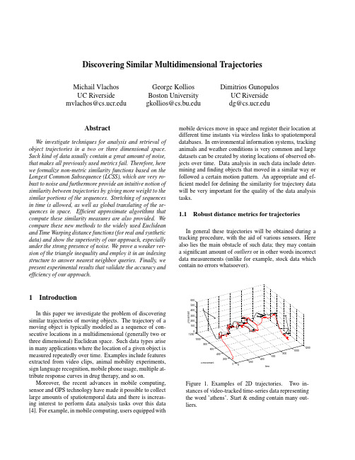
Discovering Similar Multidimensional TrajectoriesMichail VlachosUC Riverside mvlachos@George KolliosBoston Universitygkollios@Dimitrios GunopulosUC Riversidedg@AbstractWe investigate techniques for analysis and retrieval of object trajectories in a two or three dimensional space. Such kind of data usually contain a great amount of noise, that makes all previously used metrics fail.Therefore,here we formalize non-metric similarity functions based on the Longest Common Subsequence(LCSS),which are very ro-bust to noise and furthermore provide an intuitive notion of similarity between trajectories by giving more weight to the similar portions of the sequences.Stretching of sequences in time is allowed,as well as global translating of the se-quences in space.Efficient approximate algorithms that compute these similarity measures are also provided.We compare these new methods to the widely used Euclidean and Time Warping distance functions(for real and synthetic data)and show the superiority of our approach,especially under the strong presence of noise.We prove a weaker ver-sion of the triangle inequality and employ it in an indexing structure to answer nearest neighbor queries.Finally,we present experimental results that validate the accuracy and efficiency of our approach.1IntroductionIn this paper we investigate the problem of discovering similar trajectories of moving objects.The trajectory of a moving object is typically modeled as a sequence of con-secutive locations in a multidimensional(generally two or three dimensional)Euclidean space.Such data types arise in many applications where the location of a given object is measured repeatedly over time.Examples include features extracted from video clips,animal mobility experiments, sign language recognition,mobile phone usage,multiple at-tribute response curves in drug therapy,and so on.Moreover,the recent advances in mobile computing, sensor and GPS technology have made it possible to collect large amounts of spatiotemporal data and there is increas-ing interest to perform data analysis tasks over this data [4].For example,in mobile computing,users equipped with mobile devices move in space and register their location at different time instants via wireless links to spatiotemporal databases.In environmental information systems,tracking animals and weather conditions is very common and large datasets can be created by storing locations of observed ob-jects over time.Data analysis in such data include deter-mining andfinding objects that moved in a similar way or followed a certain motion pattern.An appropriate and ef-ficient model for defining the similarity for trajectory data will be very important for the quality of the data analysis tasks.1.1Robust distance metrics for trajectoriesIn general these trajectories will be obtained during a tracking procedure,with the aid of various sensors.Here also lies the main obstacle of such data;they may contain a significant amount of outliers or in other words incorrect data measurements(unlike for example,stock data which contain no errors whatsoever).Figure1.Examples of2D trajectories.Two in-stances of video-tracked time-series data representingthe word’athens’.Start&ending contain many out-liers.Athens 1Athens 2Boston 1Boston 2DTWLCSSFigure 2.Hierarchical clustering of 2D series (displayed as 1D for clariry).Left :The presence of many outliers in the beginning and the end of the sequences leads to incorrect clustering.DTW is not robust under noisy conditions.Right :The focusing on the common parts achieves the correct clustering.Our objective is the automatic classification of trajec-tories using Nearest Neighbor Classification.It has been shown that the one nearest neighbor rule has asymptotic er-ror rate that is at most twice the Bayes error rate[12].So,the problem is:given a database of trajectories and a query (not already in the database),we want to find the trajectory that is closest to .We need to define the following:1.A realistic distance function,2.An efficient indexing scheme.Previous approaches to model the similarity between time-series include the use of the Euclidean and the Dy-namic Time Warping (DTW)distance,which however are relatively sensitive to noise.Distance functions that are ro-bust to extremely noisy data will typically violate the trian-gular inequality.These functions achieve this by not consid-ering the most dissimilar parts of the objects.However,they are useful,because they represent an accurate model of the human perception,since when comparing any kind of data (images,trajectories etc),we mostly focus on the portions that are similar and we are willing to pay less attention to regions of great dissimilarity.For this kind of data we need distance functions that can address the following issues:Different Sampling Rates or different speeds.The time-series that we obtain,are not guaranteed to be the outcome of sampling at fixed time intervals.The sensors collecting the data may fail for some period of time,leading to inconsistent sampling rates.Moreover,two time series moving at exactly the similar way,but one moving at twice the speed of the other will result (most probably)to a very large Euclidean distance.Similar motions in different space regions .Objectscan move similarly,but differ in the space they move.This can easily be observed in sign language recogni-tion,if the camera is centered at different positions.If we work in Euclidean space,usually subtracting the average value of the time-series,will move the similar series closer.Outliers.Might be introduced due to anomaly in the sensor collecting the data or can be attributed to hu-man ’failure’(e.g.jerky movement during a track-ing process).In this case the Euclidean distance will completely fail and result to very large distance,even though this difference may be found in only a few points.Different lengths.Euclidean distance deals with time-series of equal length.In the case of different lengths we have to decide whether to truncate the longer series,or pad with zeros the shorter etc.In general its use gets complicated and the distance notion more vague.Efficiency.It has to be adequately expressive but suf-ficiently simple,so as to allow efficient computation of the similarity.To cope with these challenges we use the Longest Com-mon Subsequence (LCSS)model.The LCSS is a varia-tion of the edit distance.The basic idea is to match two sequences by allowing them to stretch,without rearranging the sequence of the elements but allowing some elements to be unmatched .The advantages of the LCSS method are twofold:1)Some elements may be unmatched,where in Eu-clidean and DTW all elements must be matched,even the outliers.2)The LCSS model allows a more efficient approximatecomputation,as will be shown later(whereas in DTW you need to compute some costly Norm).Infigure2we can see the clustering produced by the distance.The sequences represent data collected through a video tracking process.Originally they represent 2d series,but only one dimension is depicted here for clar-ity.The fails to distinguish the two classes of words, due to the great amount of outliers,especially in the begin-ning and in the end of the ing the Euclidean distance we obtain even worse results.The produces the most intuitive clustering as shown in the samefigure. Generally,the Euclidean distance is very sensitive to small variations in the time axis,while the major drawback of the is that it has to pair all elements of the sequences.Therefore,we use the model to define similarity measures for trajectories.Nevertheless,a simple extension of this model into2or more dimensions is not sufficient, because(for example)this model cannot deal with paral-lel movements.Therefore,we extend it in order to address similar problems.So,in our similarity model we consider a set of translations in2or more dimensions and wefind the translation that yields the optimal solution to the problem.The rest of the paper is organized as follows.In section2 we formalize the new similarity functions by extending the model.Section3demonstrates efficient algorithms to compute these functions and section4elaborates on the indexing structure.Section5provides the experimental validation of the accuracy and efficiency of the proposed approach and section6presents the related work.Finally, section7concludes the paper.2Similarity MeasuresIn this section we define similarity models that match the user perception of similar trajectories.First we give some useful definitions and then we proceed by presenting the similarity functions based on the appropriate models.We assume that objects are points that move on the-plane and time is discrete.Let and be two trajectories of moving objects with size and respectively,whereand.For a trajectory,let be the sequence.Definition1Given an integer and a real number,we define the as follows:A Ba and andThe constant controls how far in time we can go in order to match a given point from one trajectory to a point in another trajectory.The constant is the matching threshold(see figure3).Thefirst similarity function is based on the and the idea is to allow time stretching.Then,objects that are close in space at different time instants can be matched if the time instants are also close.Definition2We define the similarity function between two trajectories and,given and,as follows:Definition3Given,and the family of translations,we define the similarity function between two trajectories and,as follows:So the similarity functions and range from to. Therefore we can define the distance function between two trajectories as follows:Definition4Given,and two trajectories and we define the following distance functions:andNote that and are symmetric.is equal to and the transformation that we use in is translation which preserves the symmetric prop-erty.By allowing translations,we can detect similarities be-tween movements that are parallel in space,but not iden-tical.In addition,the model allows stretching and displacement in time,so we can detect similarities in move-ments that happen with different speeds,or at different times.Infigure4we show an example where a trajectory matches another trajectory after a translation is applied. Note that the value of parameters and are also important since they give the distance of the trajectories in space.This can be useful information when we analyze trajectory data.XFigure4.Translation of trajectory.The similarity function is a significant improvement over the,because:i)now we can detect parallel move-ments,ii)the use of normalization does not guarantee that we will get the best match between two u-ally,because of the significant amount of noise,the average value and/or the standard deviation of the time-series,that are being used in the normalization process,can be distorted leading to improper translations.3Efficient Algorithms to Compute the Simi-larity3.1Computing the similarity functionTo compute the similarity functions we have to run a computation for the two sequences.Thecan be computed by a dynamic programming algorithm in time.However we only allow matchings when the difference in the indices is at most,and this allows the use of a faster algorithm.The following lemma has been shown in[5],[11].Lemma1Given two trajectories and,with and,we canfind the in time.If is small,the dynamic programming algorithm is very efficient.However,for some applications may need to be large.For that case,we can speed-up the above computa-tion using random sampling.Given two trajectories and ,we compute two subsets and by sampling each trajectory.Then we use the dynamic programming algo-rithm to compute the on and.We can show that,with high probability,the result of the algorithm over the samples,is a good approximation of the actual value. We describe this technique in detail in[35].3.2Computing the similarity functionWe now consider the more complex similarity function .Here,given two sequences,and constants, we have tofind the translation that maximizes the length of the longest common subsequence of()over all possible translations.Let the length of trajectories and be and re-spectively.Let us also assume that the translationis the translation that,when applied to,gives a longest common subsequence,and it is also the translation that maximizes the length of the longest common subsequence.The key observation is that,although there is an infinite number of translations that we can apply to,each transla-tion results to a longest common subsequence between and,and there is afinite set of possible longest common subsequences.In this section we show that we can efficiently enumerate afinite set of translations,such that this set provably includes a translation that maximizes the length of the longest common subsequence of and .To give a bound on the number of transformations that we have to consider,we look at the projections of the two trajectories on the two axes separately.We define theprojection of a trajectoryto be the sequence of the valueson the -coordinate:.A one di-mensional translation is a function that adds a con-stant to all the elements of a 1-dimensional sequence:.Take the projections of and ,and respec-tively.We can show the following lemma:Lemma 2Given trajectories ,if ,then the length of the longest common subsequence of the one dimensional sequences and,is at least :.Also,.Now,consider and .A translation by ,applied to can be thought of as a linear transformation of the form .Such a transformation will allowto be matched to all for which ,and.It is instructive to view this as a stabbing problem:Con-sider the vertical line segments,where (Figure 5).Bx,i By,i+2Bx,i+3Bx,i+4Bx,i+5Ax,iAx,i+1Ax,i+2fc1(x) = x + c1fc2(x) = x + c2Ax axisBx axisFigure 5.An example of two translations.These line segments are on a two dimensional plane,where on the axis we put elements ofand on the axis we put elements of .For every pair of elementsin and that are within positions from eachother (and therefore can be matched by the algo-rithm if their values are within ),we create a vertical line segment that is centered at the point and extends above and below this point.Since each element in can be matched with at most elements in ,the total number of such line segments is .A translation in one dimension is a function of the form .Therefore,in the plane we de-scribed above,is a line of slope 1.After translatingby ,an element of can be matched to an el-ement of if and only if the line intersects the line segment .Therefore each line of slope 1defines a set of possi-ble matchings between the elements of sequences and.The number of intersected line segments is actually an upper bound on the length of the longest common sub-sequence because the ordering of the elements is ignored.However,two different translations can result to different longest common subsequences only if the respective lines intersect a different set of line segments.For example,the translations and in figure 5intersect different sets of line segments and result to longest common subsequences of different length.The following lemma gives a bound on the number of possible different longest common subsequences by bound-ing the number of possible different sets of line segments that are intersected by lines of slope 1.Lemma 3Given two one dimensional sequences ,,there are lines of slope 1that intersect different sets of line segments.Proof:Let be a line of slope 1.If we move this line slightly to the left or to the right,it still in-tersects the same number of line segments,unless we cross an endpoint of a line segment.In this case,the set of inter-sected line segments increases or decreases by one.There are endpoints.A line of slope 1that sweeps all the endpoints will therefore intersect at most different sets of line segments during the sweep.In addition,we can enumerate the trans-lations that produce different sets of potential matchings byfinding the lines of slope 1that pass through the endpoints.Each such translation corresponds to a line .This set of translations gives all possible matchings for a longest common subsequence of .By applying the same process on we can also find a set of translations that give all matchings of.To find the longest common subsequence of the se-quences we have to consider only thetwo dimensional translations that are created by taking the Cartesian product of the translations on and the trans-lations on .Since running the LCSS algorithm takeswe have shown the following theorem:Theorem 1Given two trajectories and,withand ,we can compute theintime.3.3An Efficient Approximate AlgorithmTheorem 1gives an exact algorithm for computing ,but this algorithm runs in cubic time.In this section we present a much more efficient approximate algorithm.The key in our technique is that we can bound the difference be-tween the sets of line segments that different lines of slope 1intersect,based on how far apart the lines are.Consider again the one dimensional projections. Lets us consider the translations that result to different sets of intersected line segments.Each translation is a line of the form.Let us sort these trans-lations by.For a given translation,let be the set of line segments it intersects.The following lemma shows that neighbor translations in this order intersect similar sets of line segments.Lemma4Let be the different translations for sequences and,where.Then the symmetric difference.We can now prove our main theorem:Theorem2Given two trajectories and,with and,and a constant,we canfind an ap-proximation of the similaritysuch that intime.Proof:Let.We consider the projections of and into the and axes.There exists a translation on only such that is a superset of the matches in the optimal of and.In addition,by the previous lemma,there are translations()that have at most different matchings from the optimal. Therefore,if we use the translations,fortime if we runpairs of translations in the plane.Since there is one that is away from the optimal in each dimension,there is one that is away from the optimal in2dimensions.Setting-th quantiles for each set,pairs of translations.4.Return the highest result.4Indexing Trajectories for Similarity Re-trievalIn this section we show how to use the hierarchical tree of a clustering algorithm in order to efficiently answer near-est neighbor queries in a dataset of trajectories.The distance function is not a metric because it does not obey the triangle inequality.Indeed,it is easy to con-struct examples where we have trajectories and, where.This makes the use of traditional indexing techniques diffi-cult.We can however prove a weaker version of the triangle inequality,which can help us avoid examining a large por-tion of the database objects.First we define:Clearly,or in terms of distance:In order to provide a lower bound we have to maximize the expression.Therefore,for every node of the tree along with the medoid we have to keep the trajectory that maximizes this expression.If the length of the query is smaller than the shortest length of the trajec-tories we are currently considering we use that,otherwise we use the minimum and maximum lengths to obtain an approximate result.4.2Searching the Index tree for Nearest Trajec-toriesWe assume that we search an index tree that contains tra-jectories with minimum length and maximum length .For simplicity we discuss the algorithm for the1-Nearest Neighbor query,where given a query trajectory we try tofind the trajectory in the set that is the most sim-ilar to.The search procedure takes as input a nodein the tree,the query and the distance to the closest tra-jectory found so far.For each of the children,we check if the child is a trajectory or a cluster.In case that it is a trajectory,we just compare its distance to with the current nearest trajectory.If it is a cluster,we check the length of the query and we choose the appropriate value for .Then we compute a lower bound to the distance of the query with any trajectory in the cluster and we compare the result with the distance of the current near-est neighbor.We need to examine this cluster only if is smaller than.In our scheme we use an approximate algorithm to compute the.Consequently,the value offrom the bound we compute for.Note that we don’t need to worry about the other terms since they have a negative sign and the approximation algorithm always underestimates the .5Experimental EvaluationWe implemented the proposed approximation and index-ing techniques as they are described in the previous sec-tions and here we present experimental results evaluating our techniques.We describe the datasets and then we con-tinue by presenting the results.The purpose of our experi-ments is twofold:first,to evaluate the efficiency and accu-racy of the approximation algorithm presented in section3 and second to evaluate the indexing technique that we dis-cussed in the previous section.Our experiments were run on a PC AMD Athlon at1GHz with1GB RAM and60 GB hard disk.5.1Time and Accuracy ExperimentsHere we present the results of some experiments using the approximation algorithm to compute the similarity func-tion.Our dataset here comes from marine mammals’satellite tracking data.It consists of sequences of geo-graphic locations of various marine animals(dolphins,sea lions,whales,etc)tracked over different periods of time, that range from one to three months(SEALS dataset).The length of the trajectories is close to.Examples have been shown infigure1.In table1we show the computed similarity between a pair of sequences in the SEALS dataset.We run the exact and the approximate algorithm for different values of and and we report here some indicative results.is the num-ber of times the approximate algorithm invokes the procedure(that is,the number of translations that we try).As we can see,for and we get very good results.We got similar results for synthetic datasets.Also, in table1we report the running times to compute the simi-larity measure between two trajectories of the same dataset. The approximation algorithm uses again from to differ-ent runs.The running time of the approximation algorithm is much faster even for.As can be observed from the experimental results,the running times of the approximation algorithm is not pro-portional to the number of runs().This is achieved by reusing the results of previous translations and terminat-ing early the execution of the current translation,if it is not going to yield a better result.The main conclusion of the above experiments is that the approximation algorithm can provide a very tractable time vs accuracy trade-off for computing the similarity between two trajectories,when the similarity is defined using the model.5.2Classification using the Approximation Algo-rithmWe compare the clustering performance of our method to the widely used Euclidean and DTW distance functions. Specifically:cover.htmlSimilarityApproximate for K tries Exact9494250.250.3160.18460.2530.00140.0022 0.50.5710.4100.5100.00140.0022 0.250.3870.1960.3060.00180.00281 0.50.6120.4880.5630.00180.00280 0.250.4080.2500.3570.001910.0031 0.50.6530.4400.5840.001930.0031 Table1.Similarity values and running times between two sequences from our SEALS dataset.1.The Euclidean distance is only defined for sequencesof the same length(and the length of our sequences vary considerably).We tried to offer the best possible comparison between every pair of sequences,by slid-ing the shorter of the two trajectories across the longer one and recording their minimum distance.2.For DTW we modified the original algorithm in orderto match both x and y coordinates.In both DTW and Euclidean we normalized the data before computing the distances.Our method does not need any normal-ization,since it computes the necessary translations.3.For LCSS we used a randomized version with andwithout sampling,and for various values of.The time and the correct clusterings represent the average values of15runs of the experiment.This is necessary due to the randomized nature of our approach.5.2.1Determining the values for&The values we used for and are clearly dependent on the application and the dataset.For most datasets we had at our disposal we discovered that setting to more than of the trajectories length did not yield significant improvement.Furthermore,after some point the similarity stabilizes to a certain value.The determination of is appli-cation dependent.In our experiments we used a value equal to the smallest standard deviation between the two trajec-tories that were examined at any time,which yielded good and intuitive results.Nevertheless,when we use the index the value of has to be the same for all pairs of trajectories.5.2.2Experiment1-Video tracking data.The2D time series obtained represent the X and Y position of a human tracking feature(e.g.tip offinger).In conjuc-tion with a”spelling program”the user can”write”various words[19].We used3recordings of5different words.The data correspond to the following words:’athens’,’berlin’,’london’,’boston’,’paris’.The average length of the series is around1100points.The shortest one is834points and the longest one1719points.To determine the efficiency of each method we per-formed hierarchical clustering after computing thepairwise distances for all three distance functions.We eval-uate the total time required by each method,as well as the quality of the clustering,based on our knowledge of whichword each trajectory actually represents.We take all possi-ble pairs of words(in this case pairs)and use the clustering algorithm to partition them into two classes.While at the lower levels of the dendrogram the clustering is subjective,the top level should provide an accurate divi-sion into two classes.We clustered using single,complete and average linkage.Since the best results for every dis-tance function are produced using the complete linkage,we report only the results for this approach(table2).The same experiment is conducted with the rest of the datasets.Exper-iments have been conducted for different sample sizes and values of(as a percentage of the original series length).The results with the Euclidean distance have many clas-sification errors and the DTW has some errors,too.For the LCSS the only real variations in the clustering are for sam-ple sizes.Still the average incorrect clusterings for these cases were constantly less than one().For 15%sampling or more,there were no errors.5.2.3Experiment2-Australian Sign LanguageDataset(ASL).The dataset consists of various parameters(such as the X,Y, Z hand position,azimuth etc)tracked while different writ-ers sign one the95words of the ASL.These series are rel-atively short(50-100points).We used only the X and Y parameters and collected5recordings of the following10 words:’Norway’,’cold’,’crazy’,’eat’,’forget’,’happy’,’innocent’,’later’,’lose’,’spend’.This is the experiment conducted also in[25](but there only one dimension was used).Examples of this dataset can be seen infigure6.Correct Clusterings(out of10)Complete Linkage Euclidean34.96DTW237.6412.7338.04116.17328.85145.06565.203113.583266.753728.277Distance Time(sec)CorrectClusterings(out of45)ASL with noiseEuclidean 2.271520Figure 7.ASL data :Time required to compute the pairwise distances of the 45combinations(same for ASL and ASL withnoise)Figure 8.Noisy ASL data :The correct clusterings of the LCSS method using complete linkage.Figure 9.Performance for increasing number of Near-est Neighbors.Figure 10.The pruning power increases along with the database size.jectories.We executed a set of -Nearest Neighbor (K-NN)queries for ,,,and and we plot the fraction of the dataset that has to be examined in order to guarantee that we have found the best match for the K-NN query.Note that in this fraction we included the medoids that we check during the search since they are also part of the dataset.In figure 9we show some results for -Nearest Neigh-bor queries.We used datasets with ,and clusters.As we can see the results indicate that the algorithm has good performance even for queries with large K.We also per-formed similar experiments where we varied the number of clusters in the datasets.As the number of clusters increased the performance of the algorithm improved considerably.This behavior is expected and it is similar to the behavior of recent proposed index structures for high dimensional data [9,6,21].On the other hand if the dataset has no clusters,the performance of the algorithm degrades,since the major-ity of the trajectories have almost the same distance to the query.This behavior follows again the same pattern of high dimensional indexing methods [6,36].The last experiment evaluates the index performance,over sets of trajectories with increasing cardinality.We in-dexed from to trajectories.The pruning power of the inequality is evident in figure 10.As the size of the database increases,we can avoid examining a larger frac-tion of the database.6Related WorkThe simplest approach to define the similarity between two sequences is to map each sequence into a vector and then use a p-norm distance to define the similarity measure.The p-norm distance between two n-dimensional vectors and is defined as。
METHOD AND APPARATUS FOR FORMING A NONWOVEN FIBROU

专利名称:METHOD AND APPARATUS FOR FORMINGA NONWOVEN FIBROUS WEB发明人:GENTILE A,US,HAUCK C,US申请号:US3772107D申请日:19711103公开号:US3772107A公开日:19731113专利内容由知识产权出版社提供摘要:A method of forming a nonwoven fibrous web from multiple laps of staple fibers, the major proportion of fibers within each lap being substantially oriented in one direction. Laps of the staple fibers are fed into overlying relationship with the major proportion of oriented fibers in each lap disposed in the same direction. Air is entrapped between adjacent laps as they are fed into overlying relationship to create an air barrier between adjacent overlying laps. The overlying laps are spread transversely of the direction in which the major proportion of fibers are oriented, and fibers within overlying laps are reoriented transversely within the plane of the laps out of the direction in which the major proportion of fibers are oriented while maintaining the air barrier between the adjacent overlying laps. The laps are pressed together after the lap spreading and fiber reorienting steps to form a unitary nonwoven fibrous web and fibers of the unitary nonwoven fibrous web are then bonded together.申请人:GENTILE A,US,HAUCK C,US更多信息请下载全文后查看。
Journal Citation Reports 中文说明书

Journal Citation Reports中文使用手冊本公司已於2010年6月25日確認此為最新版本.目次目次 (2)JCR簡介 (4)JCR的使用者 (4)直接連結JCR (5)從ISI Web of Knowledge平台進入 (5)Links from Web of Science(從WOS進入) (6)Journal Search Screen期刊搜尋畫面 (9)Journal Search Options期刊檢索項目選擇 (9)Journal Summary List 查詢結果清單 (10)Full Record Page 全記錄 (11)Journal Rank in Categories (13)Eigenfactor TM & Article Influence TM (14)Impact Factor 影響指數 (15)Five Year Impact Factors 五年影響指數 (15)Immediacy Index 立即指數 (16)Cited Half-Life 被引用半衰期 (16)Cited Journal Graph 被引用期刊圖表 (17)Citing Half-Life 引用半衰期 (17)Citing Journal Graph引用期刊圖表 (18)Source Data原始資料 (18)Cited Journal Data 被引用期刊清單 (19)Citing Journal List 引用期刊清單 (20)Related Journals 相關期刊 (21)Impact Factor Trend Graph影響指數圖表 (22)View Journals by Subject Category 以分類瀏覽期刊 (24)Sort Again再次排序 (25)View Category Data 看瀏覽資訊 (26)Journals Related to Aggregate Subject Category 學科領域的相關期刊 (29)Marking Records選取期刊 (30)Marked List個人選取清單 (31)Printing Records列印 (31)Saving Records儲存 (32)Importing Saved Records to Microsoft Excel 將儲存資料輸出到EXCEL (32)Journal Title Changes 期刊名稱變更 (35)Unified Impact Factors合併影響指數 (36)登入EndNote Web (38)建立EndNote Web中的參考文獻 (40)管理EndNote Web中的參考文獻 (42)引用EndNote Web中的參考文獻 (44)選擇書目格式 (46)編輯引用文獻 (47)移除參數 (48)Contacting Thomson Reuters (49)聯絡碩睿資訊有限公司 (49)JCR簡介Journal Citation Reports(JCR)是一個獨特的各種學科期刊評鑑工具。
单细胞混样品测序后数据拆分(CellHashing技术)

单细胞混样品测序后数据拆分(CellHashing技术)最近有学徒提到她在复现⽂献:《utative regulators for the continuum of erythroid differentiation revealed by single-cell transcriptome ofhuman BM and UCB cells.》的单细胞数据分析的时候.她发现作者明明是提到了6个样品,但是其数据集是:https:///geo/query/acc.cgi?acc=GSE150774,可以看到是5个数据:GSM4558614 CD235a+ cells - umbilical cord blood 2 and umbilical cord blood 3,UCB3GSM4558615 CD235a+ cells - umbilical cord blood 1GSM4558616 CD235a+ cells - Bone Marrow 2GSM4558617 CD235a+ cells - Bone Marrow 3GSM4558618 CD235a+ cells - Bone Marrow 4仔细看了看⽂章⾥⾯的描述,确实是 10x Genomics platform 这个技术,是 3 adult bone marrow and 3 umbilical cord blood samples ,合起来是6个样品,⽽且提前做了细胞分选,仅仅是关注 CD235a+ cells学徒以为是作者数据整理上传失败,其实是cell hashing技术,⼤家可以先去了解 CITE-seq技术,它可以同时拿到普通基因的表达量矩阵,以及⼏⼗个蛋⽩质(通过antibody-derived tags (ADT))的表达量矩阵,该技术的全称为cellular indexing of transcriptomes and epitopes by sequencing。
基于种群信息的布谷鸟算法

基于种群信息的布谷鸟算法
高淑芝;高越
【期刊名称】《沈阳化工大学学报》
【年(卷),期】2022(36)1
【摘要】布谷鸟算法(CS)是一种优秀的元启发式算法,其控制参数少的优点使它可以很容易确定控制参数和结果的关系,在许多实际问题的处理中都发挥了良好的作用.但是单一的Levy飞行策略使每个个体很难凭借自身的随机游动跳出局部极值,长时间陷入局部极小值限制了算法的收敛速度.为此,提出一种基于种群信息的布谷鸟算法(PBCS).整个种群的平均位置信息将作为个体迭代时的参考方向,使个体可以成功地跳出局部极值.将种群最优位置作为生成新个体方向,可以增加整个算法的收敛速度,便于在寻找到最优值所在的区域后迅速收敛.在6种常见的基准函数上与其他两种算法的对比,证明该算法具有更好的全局探索和局部搜索能力.
【总页数】5页(P69-73)
【作者】高淑芝;高越
【作者单位】沈阳化工大学装备可靠性研究所;沈阳化工大学信息工程学院
【正文语种】中文
【中图分类】TP18
【相关文献】
1.基于信息熵多种群遗传算法的组播路由
2.基于信息熵的异类多种群蚁群算法
3.基于信息素扩散机制的双种群蚁群优化算法
4.基于多代种群进化信息改进的差分进化算法研究
5.基于双种群布谷鸟算法的机械臂力矩最优轨迹研究
因版权原因,仅展示原文概要,查看原文内容请购买。
面向科技文献多维语义组织的混合倒排索引构建方法

面向科技文献多维语义组织的混合倒排索引构建方法
张敏;李唯;范青
【期刊名称】《现代情报》
【年(卷),期】2024(44)2
【摘要】[目的/意义]为满足科研人员对科技文献内部细粒度语义信息进行高效查询的迫切需求,前期研究提出了面向科技文献的多维语义索引体系,然而基于HashMap的常见倒排索引会导致查询效率低下。
本文旨在通过面向不同维度语义特征建立混合倒排索引,以改进语义查询性能。
[方法/过程]本文以Treap、B+树等多种数据结构探索适合不同语义维度的倒排索引构建方法,并将其组合形成多种适用于科技文献多维语义组织的混合倒排索引构建方法,并通过对比实验,在排序查询和布尔查询条件下分析验证不同类型倒排索引构建方法的查询性能。
[结果/结论]实验结果表明,组合形成的8种混合倒排索引构建方法中,表2所示的C3(HHHB)被证明在排序查询条件下具有最高的效率,而C4(TTTB)则在布尔查询条件下被证明最为高效。
本文的方法能有效解决单一索引结构导致的查询效率问题。
【总页数】9页(P107-114)
【作者】张敏;李唯;范青
【作者单位】中国科学院武汉文献情报中心;武汉软件工程职业学院(武汉开放大学);华中师范大学国家文化产业研究中心;科技大数据湖北省重点实验室
【正文语种】中文
【中图分类】G203
【相关文献】
1.面向科技文献的多模态语义关联特征提取与表达体系研究
2.基于多维语义关联的学术文献展示方法研究
3.使用倒排索引优化面向组合的语义服务发现
4.基于知识组织体系的多维语义关联数据构建研究
5.科技文献的资源语义空间:一种细粒度知识组织方法
因版权原因,仅展示原文概要,查看原文内容请购买。
- 1、下载文档前请自行甄别文档内容的完整性,平台不提供额外的编辑、内容补充、找答案等附加服务。
- 2、"仅部分预览"的文档,不可在线预览部分如存在完整性等问题,可反馈申请退款(可完整预览的文档不适用该条件!)。
- 3、如文档侵犯您的权益,请联系客服反馈,我们会尽快为您处理(人工客服工作时间:9:00-18:30)。
By means of HEX programs, powerful meta-reasoning becomes available in a decidable setting, e.g., for SemanticWeb applications, for meta-interpretation in ASP itself, or for defining policy languages. For example, advanced closed world reasoning or the definition of constructs for an extended ontology language (e.g., of RDF-Schema) is wellsupported. Due to the higher-order features, the representation is succinct. An experimental prototype implementation of the language is available, based on a reduction to ordinary ASP.
cuwovymxpu tes the predicate t taking values from the predicate
. This latter predicates extracts RDF statements from
the set of URI specified by means of § ; this task is delegated
p , "$"$3 are higher-order atoms,
are either higher-order atoms or exter-
nal atoms. The operator “AeUf ” is negation as fail-
ufw orre {m"$(o$uw"rqAwdr sej f a"ua$lr"te
An external atom facilitates to determine the truth value of an atom through an external source of computation. For in-
sta7 n¤9c8Ae@C,B$t)EhDGeFrHPuICle)RQGBTSU¨VXW¥Ya`cbed f(gih9¤98A@CB$)EDGFHPIC)RQGBTSU¨3)Pqp3r3¤§f(gs¨
DLV-HEX: Dealing with Semantic Web under Answer-Set Programming
Thomas Eiter, Giovambattista Ianni, Roman Schindlauer, and Hans Tompits Institut fu¨r Informationssysteme, Technische Universita¨t Wien,
ns edugtTav9twxio n").$$$ Awynjeez ,xtewrhnearle as to m"$$i$s s two lueist| s of terms (called input and
od f
the and
output
list, respectively), and is an external predicate name.
2 HEX Programs
HEX programs are sets of rules of the form
$""V U"$"EsdA seqf gdqhi q$"$ seqf gjk (1)
wanhdereA ql $"n$m 3gj o
whAerehigs¢he$r"-o$rd es rd
atom are
(or atom) is terms. It
a tuple s¡ v s
is possible
q$"$$ s d z ,
to specify
¥§m|¤¦ £ of©r ¥§¨le¦ cf© ¨uv l|¤e£s owf z
awto mv |¤s£
in
£
frz £a. mt ei-sloagsich-olriktceustyfnotraxth.eFcoorninjusntacnticoen,
The semaห้องสมุดไป่ตู้tics of HEX program is given by generalizing
the answer-set semantics [Eiter et al., 2005]. We note that the
answer-set semantics may yield no, one, or multiple models
However, for important issues such as meta-reasoning in the context of the Semantic Web, no adequate answer-set engines have been available so far. Motivated by this fact and the observation that, furthermore, interoperability with other software is an important issue (not only in this context), Eiter et al. [2005] extended the answer-set semantics to HEX programs, which are higher order logic programs (which accommodate meta-reasoning through higher-order atoms) with external atoms for software interoperability. Intuitively, a higher-order atom allows to quantify values over predicate names, and to freely exchange predicate symbols with constant symbols, like in the rule
F¡ aevitoerri,tieannsntri,arßoem9a–n1,1to, mA-p1i0ts4¢ 0@Vkire.ntunwa,ieAnu.asctr.aiat
Abstract
We present an implementation of HEX programs, which are nonmonotonic logic programs admitting higher-order atoms as well as external atoms. Higher-order features are widely acknowledged as useful for various tasks, including meta-reasoning. Furthermore, the possibility to exchange knowledge with external sources in a fully declarative framework such as answer-set programming (ASP) is nowadays important, in particular in view of applications in the Semantic-Web area. Through external atoms, HEX programs can deal with external knowledge and reasoners of various nature, such as RDF datasets or description-logic knowledge bases.
to an external computational source (e.g., an external deduction system, an execution library, etc.).
External atoms allow a bidirectional flow of information to and from external sources of computation such as descriptionlogic reasoners.