ANSYS三点弯曲计算报告书
ansys结构屈曲分析

退出求解器
命令: 命令:finish GUI:close the : solution menu
ANSYS 结构屈曲分析 二 结构屈曲分析的基本步骤
(3)扩展解:无论采取哪种特征值提取方法,如果想要得到屈曲模 )扩展解:无论采取哪种特征值提取方法, 态的形状,就必须执行扩展解。 态的形状,就必须执行扩展解。可以 把扩展解简单理解为将屈曲 模态的形状写入结果文件。具体操作步骤如下: 模态的形状写入结果文件。具体操作步骤如下:
注意二: 注意二: 材料的弹性模量 EX必须定义。
ANSYS 结构屈曲分析 二 结构屈曲分析的基本步骤
(2)获得静力解:与一般静力解类似,但需注意以下几点: )获得静力解:与一般静力解类似,但需注意以下几点:
注意一: 注意一:
必须激活预应力影响。 必须激活预应力影响。
注意二: 注意二:
通常只需施加一个单位荷 载即可。当施加单位荷载 载即可。 时,求解得到的特征值就 表示临界荷载, 表示临界荷载,施加非单 位荷载时, 位荷载时,求解得到的特 征值乘以施加的载荷就得 到临界荷载; 到临界荷载;
• 命令:mxpand,nmode,,,elcalc • GUI:main menu 〉solution 〉loads step opts 〉 expasionpass 〉single modes 〉expand modes
扩展求解
• 命令:solve • GUI:main menu 〉solution 〉solve 〉current LS
列出现在所有的屈曲荷载因子
命令:set,list 命令 GUI: mian menu 〉 general postproc 〉results summary
读取指定的模态来显示屈曲模态形状
ansys 屈曲分析详细过程
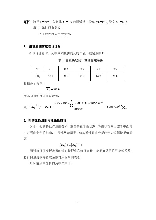
题目:跨径L=89m ,矢跨比f/L =1/5的圆弧拱,梁高h/L =1/30,梁宽b/L =1/15 求:1.弹性屈曲荷载;2.非线性极限承载能力。
1、 线性屈曲荷载理论计算在理论计算时,先根据圆弧拱的矢跨比查出稳定系数2K :表1 圆弧拱理论计算的稳定系数根据表1查得:290.4K =故其理论弹性屈曲荷载为:43723313.25105933.332966.671290.4 5.381089000xcr EI N q K m l ⨯⨯⨯⨯==⨯=⨯2、拱的弹性屈曲与非线性屈曲对于一般的特征值屈曲分析,主要是在平衡状态,考虑到轴向力或者中面内力对弯曲变形的影响,由最小势能原理,结构弹性屈曲分析归结为求解特征值问题:通过特征值分析求得的解有特征值和特征向量,特征值就是临界荷载系数,特征向量是临界荷载系数对应的屈曲模态。
特征值屈曲分析的流程图如下:[][]0D G KK λ+=图1 弹性屈曲分析流程图非线性屈曲分析是考虑结构平衡受扰动(初始缺陷、荷载扰动)的非线性静力分析,该分析是一直加载到结构极限承载状态的全过程分析,分析中可以综合考虑材料塑性和几何非线性。
结构非线性屈曲分析归结为求解矩阵方程:非线性屈曲分析的流程图如下:图2 非线性屈曲分析流程图[][](){}{}DGK K F δ+=3、非线性方程组求解方法(1)增量法增量法的实质是用分段线性的折线去代替非线性曲线。
增量法求解时将荷载分成许多级荷载增量,每次施加一个荷载增量。
在一个荷载增量中假定刚度矩阵保持不变,在不同的荷载增量中,刚度矩阵可以有不同的数值,并与应力应变关系相对应。
(2)迭代法迭代法是通过调整直线斜率对非线性曲线的逐渐逼近。
迭代法求解时每次迭代都将总荷载全部施加到结构上,取结构变形前的刚度矩阵,求得结构位移并对结构的几何形态进行修正,再用此时的刚度矩阵及位移增量求得内力增量,并进一步得到总的内力。
(3)混合法混合法是增量法和迭代法的混合使用。
工程力学三点弯曲实验报告
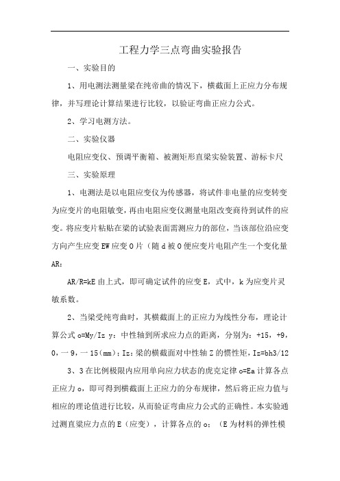
工程力学三点弯曲实验报告一、实验目的1、用电测法测量梁在纯帝曲的情况下,横截面上正应力分布规律,并写理论计算结果进行比较,以验证弯曲正应力公式。
2、学习电测方法。
二、实验仪器电阻应变仪、预调平衡箱、被测矩形直梁实验装置、游标卡尺三、实验原理1、电测法是以电阻应变仪为传感器,将试件非电量的应变转变为应变片的电阻敏变,再由电阻应变仪测量电阻改变商待到试件的应变。
将应变片粘贴在梁的试验表面需测应力的部位,当该部位沿应变方向产生应变EW应变O片(随d被O便应变片电阻产生一个变化量AR:AR/R=kE由上式,即可确定试件的应变E,式中,k为应变片灵敏系数。
2、当梁受纯弯曲时,其横截面上的正应力为线性分布,理论计算公式o=My/Iz y:中性轴到所求应力点的距离,分别为:+15,+9,0,一9,一15(mm);Iz:梁的横截面对中性轴Z的惯性矩,Iz=bh3/123、3在比例极限内应用单向应力状态的虎克定律o=Ea计算各点正应力o,即可得到横截面上正应力的分布规律,然后将正应力值与相应的理论值进行比较,从而验证弯曲应力公式的正确性。
本实验通过测直粱应力点的E(应变),计算各点的o;(E为材料的弹性模量,E=205×103MPa)4、本实验采用增量法,加载级数为4级:最终载荷(P):800N;初载荷(P。
):0N;加载级数(n):4;每级加载增量(AP):10×20=200 N;(杠杆放大倍数为20);四、实验结果相对弯曲半径越小,弯曲的变形程度越大,塑性变形在总变形中所占比重越大,因此卸载后回弹随相对弯曲半径的减小而减小,因而回弹越小。
相对弯曲半径越大,弯曲的变形程度越小,但材料断面中心部分会出现很大的弹性区,因而回弹越大;弯曲角度越大,表明变形区的长度越长,故回弹的积累值越大,其回弹角越大;材料的屈模比越大,则回弹越大。
即材料的屈服强度越大,弹性模量越小,回弹量越大。
在整个做弯曲实验过程中,基本每次都要更换凸模,我们每次都要进行调整和试模,这是比较困难的,但几次下来,也能得心应手了。
ANSYS实验分析报告

ANSYS实验分析报告专业:工程力学姓名:学号:柱体在横向作用力下的应力和变形分析第一部分:问题描述已知一矩形截面立柱,x 方向长3m ,z 方向宽2m ,y 方向高30m 。
材料为C30混凝土,弹性模量E=2.55×10¹⁰,泊松比u=0.2。
底端与地面为固定端约束,在立柱中间施加一沿x 方向的集中荷载F=30KN ,不考虑底部基础和结构自重。
如图所示:b ah柱体几何尺寸示意图理论分析:由已知条件,显然这是个弯曲问题。
根据材料力学知识,很容易知道底部与地面接触面为危险截面,左端受拉,右端受压,有:[]446max3311231015 1.51222151010.31023c c h b F pa pa ab σσ⨯⨯⨯⨯⨯⨯===⨯<=⨯⨯ []446max3311231015 1.5122215100.61023t t h bF pa pa abσσ⨯⨯⨯⨯⨯⨯===⨯<=⨯⨯ 最大变形处在顶端,挠度为:()()2323103010153330150.7351066 2.5510 4.5Z Fa f h a m EI -⨯⨯=-=⨯-=⨯⨯⨯⨯ 第二部分:ANSYS 求解过程/BATCH/input,menust,tmp,'',,,,,,,,,,,,,,,,1 WPSTYLE,,,,,,,,0 /NOPR/PMETH,OFF,0 KEYW,PR_SET,1 KEYW,PR_STRUC,1 KEYW,PR_THERM,0 KEYW,PR_FLUID,0 KEYW,PR_ELMAG,0 KEYW,MAGNOD,0 KEYW,MAGEDG,0 KEYW,MAGHFE,0 KEYW,MAGELC,0 KEYW,PR_MULTI,0 KEYW,PR_CFD,0/GO/PREP7ET,1,SOLID45 MPTEMP,,,,,,,, MPTEMP,1,0 MPDATA,EX,1,,2.55e10 MPDATA,PRXY,1,,0.2 RECTNG,0,3,0,30, VOFFST,1,2, ,FLST,5,3,4,ORDE,3 FITEM,5,7FITEM,5,-8FITEM,5,12CM,_Y,LINELSEL, , , ,P51XCM,_Y1,LINE CMSEL,,_YLESIZE,_Y1,0.5, , , , , , ,1MSHAPE,0,3DMSHKEY,1CM,_Y,VOLUVSEL, , , , 1CM,_Y1,VOLUCHKMSH,'VOLU'CMSEL,S,_YVMESH,_Y1CMDELE,_YCMDELE,_Y1CMDELE,_Y2FINISH/SOL图一.划分网格后的柱体模型图二.柱体在荷载作用下的变形图三.柱体在荷载作用下的应力第三部分:结果分析将材料力学理论计算结果与ANSYS 模拟结果进行对比:柱体最大挠度发生在顶端,理论计算结果为max f =0.735㎜,ANSYS 模拟结果为max f =0.741㎜,可见ANSYS 模拟结果是正确的。
ansys屈曲分析

3.1 几何非线性3.1.1 大应变效应一个结构的总刚度依赖于它的组成部件(单元)的方向和单刚。
当一个单元的结点经历位移后,那个单元对总体结构刚度的贡献可以以两种方式改变。
首先,如果这个单元的形状改变,它的单元刚度将改变(图3-1(a))。
其次,如果这个单元的取向改变,它的局部刚度转化到全局部件的变换也将改变(图3-1(b))。
小的变形和小的应变分析假定位移小到足够使所得到的刚度改变无足轻重。
这种刚度不变假定意味着使用基于最初几何形状的结构刚度的一次迭代足以计算出小变形分析中的位移(什么时候使用“小”变形和应变依赖于特定分析中要求的精度等级)。
相反,大应变分析考虑由单元的形状和取向改变导致的刚度改变。
因为刚度受位移影响,且反之亦然,所以在大应变分析中需要迭代求解来得到正确的位移。
通过发出 NLGEOM,ON(GUI路径Main Menu>Solution>Analysis Options),来激活大应变效应。
这种效应改变单元的形状和取向,且还随单元转动表面载荷。
(集中载荷和惯性载荷保持它们最初的方向。
)在大多数实体单元(包括所有的大应变和超弹性单元),以及部分的壳单元中大应变特性是可用的。
在ANSYS/Linear Plus程序中大应变效应是不可用的。
图3-1 大应变和大转动大应变过程对单元所承受的总旋度或应变没有理论限制。
(某些ANSYS单元类型将受到总应变的实际限制──参看下面。
)然而,应限制应变增量以保持精度。
因此,总载荷应当被分成几个较小的步,这可用〔 NSUBST, DELTIM, AUTOTS〕命令自动实现(通过GUI路径 MainMenu>Solution>Time/Frequent)。
无论何时如果系统是非保守系统,如在模型中有塑性或摩擦,或者有多个大位移解存在,如具有突然转换现象,使用小的载荷增量具有双重重要性。
3.1.2 应力-应变在大应变求解中,所有应力─应变输入和结果将依据真实应力和真实(或对数)应变(一维时,真实应变将表示为ε=Ln(l/l) 。
ANSYS的实验报告
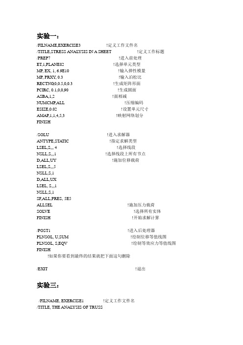
实验一:/FILNAME,EXERCISE3 !定义工作文件名/TITLE,STRESS ANAL YSIS IN A SHEET !定义工作标题/PREP7 !进入前处理ET,1,PLANE82 !选择单元类型MP, EX, 1, 6.9E10 !输入弹性模量MP, PRXY, 0.3 !输入泊松比RECTNG,0,0.5,0,0.3 !生成矩阵形面PCIRC, 0.1,0,0,90 !生成圆面ASBA,1,2 !面相减NUMCMP,ALL !压缩编码ESIZE,0.02 !设置单元尺寸AMAP,1,1,4,5,3 !映射网络划分FINISH/SOLU !进入求解器ANTYPE,STATIC !指定求解类型LSEL,S,,, 4 !选择线段NSLL,S,,,1 !选择线段上所有节点D,ALL,UY !施加位移载荷LSEL,S,,,5NSLL,S,1D,ALL,UXLSEL, S,,,1NSLL,S,1SF,ALL,PRES,-5E5ALLSEL !施加压力载荷SOLVE !选择所有实体FINISH !开始求解计算/POST1 !进入后处理器PLNSOL, U,SUM !绘制位移等值线图PLNSOL, S,EQV !绘制等效应力等值线图FINISH!如果你要看到最终的结果就把下面这句删除/EXIT !退出实验三:/FILNAME, EXERCISE1 !定义工作文件名/TITLE, THE ANAL YSIS OF TRUSS/PREP7ET,1,LINK1R,1,6E-4R,2,9E-4R,3,4E-4MP,EX,1,2.2E11MP,PRXY,1,0.3MP,EX,2,6.8E10MP,PRXY,2,0.26MP,EX,3,2.0E11MP,PRXY,3,0.26K,1,0,0,0K,2,0.8,0,0K,3,0,0.6,0/PNUM,KP,1/PNUM,LINK,1L,1,2L,2,3L,3,1/TITLE,GEOMETRIC MODEL LPLOTESIZE,,1MA T,1REAL,1LMESH,1LPLOTMA T,2REAL,2LMESH,2LPLOTMA T,3REAL,3LMESH,3FINISH/SOLUANTYPE,STATIC/PNUM,NODE,1EPLOTD,1,ALLD,3,ALLF,2,FX,3000F,2,FY,-2000SOLVEFINISH/POST1PLDISP,1PLNSOL,U,SUMPRNSOL,U,COMPPRRSOLFINISH第四个实验的源代码:/FILNAM,EX2-5/TITLE,CANTILERVER BEAM DEFLECTION/UNITS,SI/PREP7!进入前处理器ET,1, BEAM3 ! 梁单元MP, EX,1, 200E9 ! 弹性模量E=200E9 N/ m2R,1,3E-4, 2.5E-9, 0.01 ! A=3E-4 m2, I=2.5E-9 m4, H=0.01 m N,1,0,0 $ N,2, 1, 0 ! 定义节点坐标N,3, 2, 0 $ N,4,3,0 $ N,5,4,0E, 1,2 $ E,2,3 $E, 3, 4 $ E,4,5 ! 定义单元FINISH/SOLU !进入求解处理器ANTYPE, STATICD,1,ALL,0 !全固约束节点(边界处理)F,3,FY,-2 ! 施加集中载荷SFBEAM,3,1,PRES,0.05,0.05!施加均布载荷SFBEAM,4,1,PRES,0.05,0.05SOLVEFINISH/POST1!进入一般后处理器SET,1,1 !读取阶段负载答案PLDISP !显示数据列表(列出变形资料)PRDISP !显示图形列表(检查变形图)FINISH第一个实验输出的结果图:实验三的结果:第四个实验的结果:。
ansys报告

简单台柱静力分析一、问题提出一工程用圆柱形金属支柱,咼约为25m 底面直径约为3m 其底座固定在地 基上,使用中主要受载来自于顶部结构的垂直向压力为 1000N 侧向风载荷约为 100N 。
金属支柱材料弹性模量为210GPa 泊松比为0.3。
试分析其使用过程中的 变形和危险点。
二、建模步骤1.建立工作文件名个工作标题 1) .定义工作文件名依次单击:Utility Menu^File — ChangeJobname 弹出 “ChangeJobname ”对话框,如图1所示,在“ [/FILNAM]Enter newjobname ”选项的输入栏中输入 工作文件名为“ EX2-T ,勾选“ New log and error files ”选项的“ Yes ”复选 框,单击“ OK 按钮关闭该对话框。
A change JobnameE/FIlLNAM] Ent&r newjobnamt New log and error files?Cancel17 Yes0<2).定义工作标题依次单击:Utility Meni—File —Change Title,弹出“ Change Title ”对话框,如图2所示,在“ [/TITLE]Enter newtitle ”选项的输入栏中输入“ The an alysis of a cyli nder body ”,单击“OK按钮关闭该对话框。
A Change TitleI/TITLE] Enter new title The analysis of a cylinder body 1Z45523115OK Cancel2.定义单元类型3.依次单击:Main Menu —Preprocessor —Element Type —Add/Edit/Delete ,弹出“Element Types”对话框,如图3所示。
单击“Add... ”按钮,弹出“Librarty ofElement Types ” 对话框,如图 4 所示。
Ansys实验指导书 附带详细步骤
接三个特征点,1(0,0), 2(1,0),3(2,0) →OK 7.网格划分
选取方向关键点(参考点) ANSYS Main Menu: Preprocessor →Meshing →Mesh Attributes →Picked lines →拾取线 1 和 2→
OK → 在 Pick Orientation Keypoint(s)选项框选 YES→拾取:4#参考点(0,1,0) →OK 单元尺寸设置、网格划分
3
生成特征点 ANSYS Main Menu: Preprocessor →Modeling →Create →Keypoints →In Active CS →依次输入
三个点的坐标:1(0,0),2(1,0),3(2,0)及参考点的坐标 4(0,1,0) →OK 生成梁 ANSYS Main Menu: Preprocessor →Modeling →Create →Lines →lines →Straight lines →依次连
分别给 1,2,3 三个特征点施加 x 和 y 方向的约束 ANSYS Main Menu: Solution → Define Loads → Apply → Structural → Displacement → On
Keypoints →拾取 1(1,1),2(2,1),3(3,1)三个特征点 →OK →select Lab2:UX, UY → OK 给 4#特征点施加 y 方向载荷 ANSYS Main Menu: Solution → Define Loads → Apply → Structural → Force/Moment → On
ANSYS 圆管屈曲分析实验报告1

圆管屈曲分析实验报告1、问题描述图1为一薄壁圆管,壁厚为0.216m,直径为4m,高度为21.6m。
圆管的材料弹性模量为210Gpa,泊松比为0.3。
圆管两端面受约束,试分析此薄壁圆管侧壁四周受压情况下的屈曲临界载荷。
图1 薄壁圆管模型2、问题分析2.1、什么是模态及本题的模态阶数选取模态是机械结构的固有振动特性,每一个模态具有特定的固有频率、阻尼比和模态振型。
通过模态分析可以得出物体在某一易受影响的频率范围内各阶主要模态的特性,就可以预知结构在此频段内,在外部或内部各种振源作用下实际振动反应。
因此,模态分析是结构动态设计及设备的故障诊断的重要方法。
一个物体有很多固有振动频率(理论上是无穷多个),按照从小到大的顺序,第一个就叫一阶固有频率,以此类推。
模态的阶数对应固有频率阶数。
一般,低阶模态刚度相对比较弱,在同样量级的激励作用下,响应会相对所占的权值大一些,所以工程上低阶模态比较受关注,理论上低阶模态理论也相对成熟。
且用有限元进行模态分析计算,阶数越高,误差越大。
此题中分析对象比较简单,所以选取前5模态进行分析已经满足工程需要。
2.2、网格单元的选取此薄壁圆管由于壁厚远远小于直径,均匀壁厚,材料结构简单,所以单元类型可以选用shell 93—八节点结构壳单元。
2.3、网格划分类型的选取有限元分析的精度和效率与单元的密度和几何形状有密切关系,按照相应的误差准则和网格疏密程度,应该避免网格的畸形,因此,划分网格时,应尽量采用映射网格模式划分。
本题中,圆管形状规则,采取映射网格进行划分。
3、解题步骤3.1、建立工作文件名及工作标题选择Utility Menu→File→Change Jobname ,出现Change Jobname对话框,在Enter new jobname输入栏中输入工作文件名Tube, 点OK完成设置。
选择Utility Menu→File→Change Title,出现Change Title对话框,在输入栏中输入Buckling of a tube, 点OK, 完成设置。
基于ANSYS软件的压力容器屈曲分析
关于分析类型 3 之所以可以采用 ASMEⅧ-2[7-9]5.2.4 节的弹-塑性应力分析来完成,原 因是薄壁结构的非线性屈曲分析实际上是几何非线性理论在工程应用中的衍生。非线性稳 定性问题和几何非线性问题的求解方程是完全一样的。因此,从非线性角度来看,结构刚 强、度和稳定性是紧密联系在一起的。当前,有限元软件和计算机迅猛发展,以非线性理 论为基础的有限元法已成为求解板壳结构屈曲、 后屈曲及破坏的最精确最有效的途径之一。 2.3.2 欧盟直接法中的稳定性校核方法 欧 盟 新 一 代 压 力 容 器 规 范 EN13445[12,13] 在 其 附 录 B 直 接 法 中 也 给 出 屈 曲 设 计 (EN13445[12,13]中称为稳定性校核)方法。与 ASMEⅧ-2[7-9]中分析类型 3 所述方法接近, 如都考虑几何非线性的影响。该法基于下列假设: 非线性运动关系和大变形理论; 弹性理想塑性本构关系 Von Mises 屈服条件和与之相关的流动准则 无初始应力状态 给定初始几何缺陷
2.3
基于数值计算的设计方法
上述两种方法都属于规则设计(Design by rules)范畴,都有一定的适用范围,如 2.1 节所述方法要求直径厚度比 D0 / t 1000 ,2.2 节所述方法直径厚度比扩大至
D0 / t 2000 。对那些结构超出规则设计适用范围,承受局部压缩载荷的情况可采用基于
得到精确的结果。方法之一是屈曲载荷系数归一化,即不断调整变载荷,直到屈曲载荷系 数等 1.0 或接近 1.0,此时的变载荷就是结构的屈曲载荷。
3.2
避免屈曲模式丢失
进行数值分析时,应计及所有可能的失稳模式。要注意保证模型的简化不会造成屈曲 模式的丢失。尽量不要使用对称建模,以免遗漏非对称屈曲模式。例如,对经环向加强的 圆筒,在确定其最小屈曲载荷时,应考虑轴对称和非轴对称屈曲模式。
ansys弧长
3.2.2 问题详细说明下列材料性质应用于这个问题:EX=1000 (杨氏模量)NUXY=0.35(泊松比)Yield Strength =1 (屈服强度)Tang Mod=2.99(剪切模量)3.2.3 问题描述图图3-4 问题描述图3.2.4 求解步骤(GUI方法)步骤一:建立模型,给定边界条件。
在这一步中,建立计算分析所需要的模型,定义单元类型,材料性质划分网格,给定边界条件。
并将数据库文件保存为“exercise1.db”。
在此,对这一步的过程不作详细叙述(您也可以从§3.2.5中取出命令流段完成这一步骤)。
步骤二:恢复数据库文件“exercise.db”Utility Menu>File>Resume from步骤三:进入求解器。
Main Menu>solution步骤四:定义分析类型和选项1、选择菜单路径Main Menu>Solution>-Analysis Type-New Analysis.单击“Static”来选中它然后单击OK。
2、择菜单路径Main Menu>Solution>Unabridged Menu>Analysis Options。
出现对话框。
3、单击Large deform effects (大变型效应选项)使之为ON,然后单击OK。
步骤五:打开预测器。
Main menu> Solution>Unabridged Menu>Load step opts-Nonlinear> Predictor步骤六:在结点14的Y方向施加一个大小为-0.3的位移Main menu >Solution -Load -Apply >displacement >On Nodes步骤七:设置载荷步选项1、选择菜单路径Main Menu> Solution>Unabridged Menu>Load stepopts-Time/Frequenc> Time and substps。
三维弯曲梁分析实例
-3-
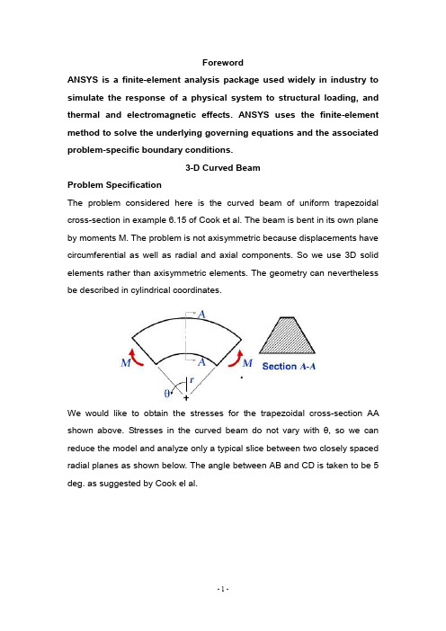
Close the Element Types dialog box and also the Element Type menu. Specify Element Constants Main Menu > Preprocessor> Real Constants > Add/Edit/Delete > Add... This brings up the Element Type for Real Constants menu with a list of the element types defined in the previous step. We have only one element type and it is automatically selected. Click OK. You should get a note saying "Please check and change keyopt setting for element SOLID45 before proceeding." This means that there are no real constants to be specified for this element, as you might recall from the plate tutorial. Close the Real Constants menu. Save Your Work Toolbar > SAVE_DB Step 3: Specify material properties Main Menu > Preprocessor > Material Props > Material Models In the Define Material Model Behavior menu, double-click on Structural, Linear, Elastic, and Isotropic.
ANSYS分析结果汇报
ANSYS建模分析报告书课题名称ANSYS建模分析姓名学号院系专业指导老师问题描述在ANSYS中建立如图一所示的支承图,假定平面支架沿厚度方向受力均匀,支承架厚度为3mm。
支承架由钢制成,钢的弹性模量为200Gpa,泊松比为0.3。
支承架左侧边被固定,沿支承架顶面施加均匀载荷,载荷与支架共平面,载荷大小为2000N/m。
要求:绘制变形图,节点位移,分析支架的主应力与等效应力。
图1GUI操作步骤1、定义工作文件名和工作标题(1)定义工作文件名:执行Utility Menu>File>Change Jobname命令,在弹出【Change Jobname】对话框中输入“xuhao144139240174”。
选择【New log and error files】复选框,单击OK按钮。
(2)定义工作标题:执行Utility Menu>File>Change Title命令,在弹出【Change Title】对话框中输入“This is analysis made by“xh144139240174”,单击OK按钮。
(3)重新显示:执行Utility Menu>Plot>Replot命令。
(4)关闭三角坐标符号:执行Utility Menu>PlotCtrls>Window Options命令,弹出【Window Options】对话框。
在【Location of triad】下拉列表框中选择“Not Shown”选项,单击OK按钮。
2、定义单元类型和材料属性(1)选择单元类型:执行Main Menu>Preprocessor>ElementType>Add/Edit/Delete命令,弹出【Element Type】对话框。
单击Add...按钮,弹出【Library of Element Types】对话框。
选择“Structural Solid”和“Quad 8node 82”选项,单击OK按钮,然后单击Close按钮。
ansys屈曲分析报告

ANSYS屈曲分析报告1. 引言本报告旨在使用ANSYS软件进行屈曲分析,并对结果进行解释和分析。
屈曲分析是一种重要的工程分析方法,用于确定结构在受力作用下的稳定性能。
在本次分析中,我们将针对特定的结构进行屈曲分析,以评估其在实际应用中的可靠性和稳定性。
2. 分析模型本次分析使用的模型是一个具有特定几何形状和材料属性的结构。
具体的几何形状和材料属性将在下文中详细介绍。
3. 材料属性为了进行准确的屈曲分析,我们需要了解材料的力学性质。
在本次分析中,我们假设材料为均匀各向同性的弹性材料。
材料的力学性质如下:•弹性模量:E = XXX GPa•泊松比:ν = XXX•密度:ρ = XXX kg/m^34. 几何模型本次分析使用的结构模型的几何形状如下所示:(此处以文字描述结构模型的几何形状)5. 约束条件和加载在进行屈曲分析时,我们需要为结构模型设置适当的约束条件和加载。
在本次分析中,我们假设结构的底部固定,并在顶部施加垂直向下的集中力。
施加的加载大小为XXX N。
6. 分析步骤屈曲分析可以通过逐步增加加载的方法进行。
在本次分析中,我们将使用以下步骤进行屈曲分析:1.施加约束条件和加载;2.进行线性静力分析,确定结构的初始状态;3.逐步增加加载,进行非线性分析,直到发生屈曲现象;4.记录并分析屈曲点。
7. 分析结果与讨论经过屈曲分析后,我们得到了以下结果:•屈曲载荷:XXX N•屈曲模态:X 模态•屈曲形状:(此处以文字描述屈曲形状的特征)根据分析结果,我们可以得出以下结论和讨论:•结构在受到XXX N的载荷时,发生了屈曲现象;•屈曲模态X是结构的主要屈曲模态,表示了结构在该模态下的变形形态;•屈曲形状的特征表明结构在屈曲时出现了X类型的失稳现象。
8. 结论本次屈曲分析报告对特定结构进行了屈曲分析,并得出了结构的屈曲载荷、屈曲模态和屈曲形状的结果。
根据分析结果,我们可以评估结构在实际应用中的可靠性和稳定性,并采取相应的措施来改进和优化结构设计。
实验三简支梁的变形Ansys分析
实验三简支梁的变形分析实验目的:了解和掌握简支梁的变形分析的方法和步骤。
实验内容:完成工字梁端面受力分析。
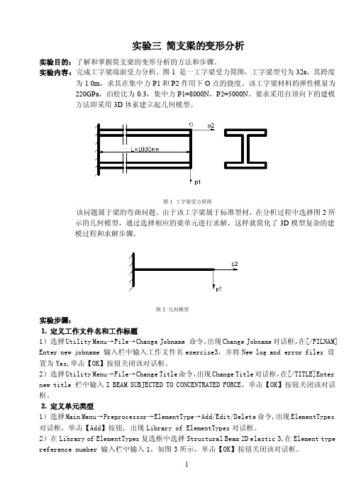
图1 是一工字梁受力简图,工字梁型号为32a,其跨度为1.0m,求其在集中力P1和P2作用下O点的挠度。
该工字梁材料的弹性模量为220GPa,泊松比为0.3,集中力P1=8000N,P2=5000N。
要求采用自顶向下的建模方法即采用3D体素建立起几何模型。
图1 工字梁受力简图该问题属于梁的弯曲问题。
由于该工字梁属于标准型材,在分析过程中选择图2所示的几何模型,通过选择相应的梁单元进行求解,这样就简化了3D模型复杂的建模过程和求解步骤。
图2 几何模型实验步骤:⒈定义工作文件名和工作标题1)选择Utility Menu→File→Change Jobname 命令,出现Change Jobname对话框,在[/FILNAM] Enter new jobname 输入栏中输入工作文件名exercise3,并将New log and error files 设置为Yes,单击【OK】按钮关闭该对话框。
2)选择Utility Menu→File→Change Title命令,出现Change Title对话框,在[/TITLE]Enter new title 栏中输入I BEAM SUBJECTED TO CONCENTRATED FORCE,单击【OK】按钮关闭该对话框。
⒉定义单元类型1)选择Main Menu→Preprocessor→ElementType→Add/Edit/Delete命令,出现ElementTypes 对话框,单击【Add】按钮, 出现Library of ElementTypes对话框。
2)在Library of ElementTypes复选框中选择Structural Beam 2D elastic 3,在Element type reference number 输入栏中输入1,如图3所示,单击【OK】按钮关闭该对话框。
ansys屈曲(Ansysbuckling)

ansys屈曲(Ansys buckling)03 string stability calculation (ANSYS)This example will discuss the eigenvalue instability and nonlinear instability of the string with prestressed stressKnowledge points:(a) prestressed(b) stable eigenvalues(c) consideration of the stability of eigenvalues of other internal forces(d) add initial defect(e) arc n(f) nonlinear analysis and convergence(g) relationship of load displacement(1) set the Parameters of analysis. In the top menu of ANSYS, parameter-> Scalar Parameters, input in the pop-up Scalar Parameters window, FORCE = 100, OFFSET = 0.1.(2) establish a model. In this example, we will contact two new units, three-dimensional Beam unit Beam 4 and 3d cable unit Link 10. The Beam 4 unit is simpler than the Beam 188 unit introduced before, and is also a useful unit for the common rectangularelastic cross section. Link 10 is the space cable unit provided by ANSYS. The user can control the unit only under pressure or can only be pulled. By default, the unit can only be pulled.(3) select Beam 4 units and Link 10 units in the ANSYS main menu Preprocessor - > Element type - > Add/Edit/Delete(4) both Beam 4 and Link 10 can use real parameters to set the section properties. First, the section of the Beam 4 unit is set. The cross section we want to build is a rectangular section of 0.1 m by 0.12 m. If the Beam 4 unit does not specify the direction of the main axis of the section, the Y-axis of the partial coordinate system of the section will be parallel to the x-y plane of the whole coordinate system. In the ANSYS main menu Preprocessor - > Real Constants - > Add/Edit/Delete, select Add, the associated unit type of the specified Real parameter is Beam 4 unit, and the input section parameter is AREA: 0.1 * 0.12, IZZ: 0.12 * 0.1 * * 3/12, IYY: 0.1 * 0.12 * 3/12, TKZ: 0.12, TKY: 0.1, as shown in the figure below(5) continue to add the second real parameter type, and specify that the second real parameter is associated with the Link 10 unit. The sectional area of the Link 10 unit is 4 x 10⁻⁶m2, and the initial strain is 2 x 10⁻³. The initial strain is the strain of strain.(6) the material properties are set below. In this example, all materials are set as steel for simplicity. Add Material properties to the ANSYS main menu Preprocessor - > Material Props - > Material Models. In the Material window, select the Structural - > Linear - > Elastic - > Isotropic, input Elasticmodulus 2 x 10⁹ and poisson ratio 0.27, also can input the Density of the Material, select the Structural - > Density in the Material window, and the input Density is 7800.(7) the geometric model is established. In this example, we still construct geometric models strictly according to the points, lines, planes and body topologies that are required by the modeling process of ANSYS.(8) the key points are established In the ANSYS main menu Preprocessor - > Modeling - > Create - > Keypoints - > In Active CS(9) connect the key points below and connect the following key points in the ANSYS main menu Preprocessor - > Modeling - > create-> Lines - > Straight LineGet the string model(10) to divide the grid by geometry. In the ANSYS main menu Preprocessor - > meshing-> Mesh Attributes - >, line 1, select 1 ~ 6 straight line, setting its unit type, material type and real parameter are all 1. Select the line 7-14, the material type is 1, the unit type and the real parameter are both 2.(11) control the size of the grid. For the analysis, in the middle of the column is the key of the research, the mesh so we want to have to close some, in the ANSYS Preprocessor main menu - > Meshing - > Size Cntrls - > Lines - > Picked Lines, select 1 ~ 6 straight Lines, set the maximum Length of grid unit (Element Edge Length) of 0.3. For the surrounding prestressedcables,Since Link 10 is a relatively complex nonlinear unit, it is easy to solve the difficult convergence problem when solving the problem. Therefore, we divide the prestressed cable into one unit. Select the line 7 ~ 14, and set the number of grid segments as 1.(12) in the ANSYS main menu Preprocessor - > meshing-> Mesh - > Lines, select all the Lines and divide the grid(13) at the top of ANSYS, the menu plotctrls-> Style -- > Size and shape, set Display of element as On. Get the unit shape as shown in the figure:(14) the boundary condition and load are added under the model. Main menu first into the ANSYS Solution - > Define Loads - > Apply - > Structural - > below - > On Keypoints, selected key point 3, constraint three horizontal movement dof UX, UY, offers and rotational degree of freedom ROTZ, select the point 2, two translational degree of freedom UX and UY constraints.(15) enter the ANSYS main menu Solution - > Define Loads - > Apply - > struck-> Force/Moment - > One Keypoints, select key point 2, load direction of FZ and size - Force(16) to conduct a Static Analysis, Solution main menu - > into ANSYS Analysis Type - > New Analysis, set for the Static Analysis of types, into the Solution - > Analysis Type - > Sol 'n Controls, set for small deformation Analysis and consider prestressed, close the automatic time step control steps andset Analysis child (Substeps) to 1(17) for a Solution operation, enter the ANSYS main menu Solution - > Solve - > Current LS.(18) the eigenvalue buckling of the model is solved. Solution main menu - > into ANSYS Analysis Type - > New Analysis, set Analysis of Type Eigen Buckling, Solution main menu - > into ANSYS Analysis Type - > Analysis Options, set the Solution of the first-order stable load.(19) to Solve the operation again, enter the ANSYS main menu Solution - > Solve - > Current LS.(20) into the post-processing operation at this moment, the main menu into ANSYS General Postproc - > Read the results - > the Last Set, Read in the Last step as a result, the main menu select ANSYS General Postproc - > Plot results - > Deformed Shape, they can get form of instability of the structure and the corresponding buckling load magnification, which is 118.602, as shown.(21) enter the Parameters - > Get scalar data at the top of ANSYS, select Results data in Get scalar data, and select Model Results (modal result) in the result, as shown in the figure. Click OK to go to the next window Get Model Results, and select the variable that will store the modal result in the name Freq1. Modal is the first order mode.(22) from the top window of the ANSYS window, the first-order frequency is 118.6021, as shown in the figure(23) the above process is the general process of analyzing eigenvalue instability. However, ANSYS has a defect in the process of analyzing eigenvalues instability. As is known to all, the so-called eigenvalue buckling calculation is to use the structure stiffness matrix minus the geometric stiffness of the structure under load multiplied by a coefficient, when the total stiffness matrix singularity is buckling eigenvalues. ANSYS in dealing with a load caused by stiffness matrix cannot differentiate between we need analysis of the external force load (in this case is top concentration) and don't need the structure of the internal force (for example, the calculation of prestressed) contribution to the geometric stiffness matrix. Therefore, it is incorrect to get the eigenvalue yield of 118602N (equal to the initial value of the initial value of 100 x eigenvalue instability of 118.602). Therefore, the problem must be solved through the following iterative calculation.(24) the basic idea of iterative calculation is to adjust the external load on the structure and to solve the eigenvalue instability magnification of the new load according to the magnification of the load.Repeat the above operation until the magnification of the eigenvalue instability is basically equal to 1. The external load added to the structure is the real eigenvalue instability load. And it doesn't contradict the internal forces. The command flow for iterative computing is as follows:! Set the maximum number of iterations 100 times* to DO, I, 1100,FINISH/ SOLU! Apply new load to the structureFk1 - FK, 2, FZ - FORCE! Static analysisANTYPE, 0! Set time1 TIME,AUTOTS, 0NSUBST, 1,,, 1SSTIF, ONSOLVEFINISH! The eigenvalue instability analysis is carried out / SOLUANTYPE, BUCKLE! Buckling analysisBUCOPT, LANB, 1! Use Block Lanczos solution method, extract 1 modeMXPAND, 1! Expand 1 mode shapePSTRES, ON! The INCLUDE PRESTRESS EFFECTSSOLVEFINISH! The first order frequency of the current eigenvalue instability (magnification)* GET FREQ1, MODE, 1, FREQ* the IF, ABS (FREQ1-1), LT, 0.01, THEN! If the frequency error is less than 1%, exit the loop* the EXIT* ENDIFThe FORCE = FORCE * FREQ1! Otherwise, the load times the new magnification is calculated again* ENDDO(25) after repeating the above process, the structure of real eigenvalue buckling load of 198174 n, visible if does not exclude the prestressed internal force of the influence of the geometric stiffness matrix, calculated the eigenvalue buckling load (118602 n) are much smaller.(26) finally, we have a nonlinear buckling analysis. The buckling load calculated by eigenvalue instability is actually the upper limit solution for ideal material. Due to various initial defects or nonlinear effects of materials, the instability load of the actual structure is usually smaller than that of the eigenvalue. Therefore, nonlinear instability analysis is necessary. In nonlinear instability analysis, initial defects need to be introduced. There are many ways to choose the initial defect, and it is more commonly used to add the eigenvalue instability shape of the structure as the most unfavorable initial defect to the structure. The UPGEOM command is provided in ANSYS to facilitate the implementation of the above process, as described below(27), first of all, we need to get the largest eigenvalue buckling mode of the structure deformation is how much, the first main menu in the ANSYS General Postpro Results - > - > List are Sorted Listing - > Sort Nodes, choose the Results of the total displacement (USUM), the maximal displacement of all Nodes.(28) next, select Parameters - > Get Scalar Data in the top menu of ANSYS and select Results Data - > Other operations in Get Scalar Data(29) in the Get Data from Other POST1 Operations window, select the Data from the sorting result that you just did. The required data is the maximum of the sorted order, which is placed in the DMAX variable.(30) DMAX = 1 can be seen from the Scalar Parameter window(31) use the UPGEOM command to adjust the shape of the structure and apply the initial defect. Select Preprocessor - > Modeling - > Update Geom in the ANSYS main menu. UPGEOM will read the structure from the result file and adjust the geometry of the structure. We set the magnification multiple as OFFSET/DMAX, i.e. the maximum initial defect we need is OFFSET = 0.1, and the maximum deformation in the result file is DMAX, so the magnification ratio is OFFSET/DMAX. Finally, the result of the specified eigenvalue instability analysis is called Case03. RST.(32) after the geometry of the structure has been updated, the nonlinear solution can be performed. We know that the load of the eigenvalue instability of the structure is 198174N, and the maximum load of the structure is the loss of the stability load of the characteristic value of three times, which is the input field in the top of the ANSYS window. The load loading structure is constructed, and the analysis type is set to static analysis.(33) in the end, we have to set the solution method in the solver control.This will automatically track the failure path. Enter the ANSYS main menu Solution - > Analysis Type - > Analysis Options. First,set the Analysis Type in the basic option to analyze the large displacement, and consider the prestress. Set the analysis substeps for 20 steps and output the results per step.(34) select the Advanced NL page in the Solution Controls window, and click on the arc-length Method, which USES the default values for the arc-length Method.Main menu (35) into ANSYS Solution - > Solve - > Current LS, began to calculate the Current problem, because the problem is that we come into contact with the first nonlinear problem, it is necessary to introduce the meaning of the output in ANSYS nonlinear calculation window. Nonlinear computing as we know, there is a convergence problem, in this example, the ANSYS output in the reprocessing window four computing intermediate variables: 2 norm of unbalanced force (F L2), unbalanced force closed then poor (F CRIT), 2 norm of unbalanced moment of L2 (M) and the unbalanced moment then sent CRIT (M). The horizontal axis in the window is the time (calculation process), and the ordinate is the corresponding value. In the case of force, if the two norm of the unbalanced force (F L2) is higher than the unbalance force, the F CRIT indicates that there is no convergence, and the calculation is to be continued. If (F L2) is less than (F CRIT), the two curves of (F L2) and (F CRIT) in the graph intersect, indicating that the step calculation has been convergent and the next load step can be calculated. In this case, the case of convergence is still good, and the general iteration converges once or twice.(36) after the calculation has been completed, the post-stroke processor enters ANSYS, selects TimeHist Postpro, and clicksthe variable button in the toolbar in Time History Variables to select add node Z direction deformation, as shown in the figure. Select node 2.(37) in the Time History Variables window set for UZ_2 X coordinates, Time to light up as Y-axis, click on the plot button on the toolbar, you can get the relative load as shown - vertex deformation curve.In General Postproc, the General Postproc - > Read Results - > By Time/Freq was selected, and the display Time was 0.2 (i.e. the maximum load equivalent to 1/5), and the General Postproc - > Plot Results - > Deformed Shape of ANSYS main menu was selected. Draw the current deformation of the structure as shown. Gradually increase the result Time, showing the deformation of Time = 0.4 and 0.6.。
ANSYS屈曲分析总结

ANSYS屈曲分析总结《ANSYS屈曲分析总结》很多现有的ANSYS资料都对特征值屈曲分析进行了较为详细的解释,特征值屈曲分析属于线性分析,它对结构临界失稳力的预测往往要高于结构实际的临界失稳力,因此在实际的工程结构分析时一般不用特征值屈曲分析。
但特征值屈曲分析作为非线性屈曲分析的初步评估作用是非常有用的。
1. 非线性屈曲分析的第一步最好进行特征值屈曲分析,特征值屈曲分析能够预测临界失稳力的大致所在,因此在做非线性屈曲分析时所加力的大小便有了依据。
特征值屈曲分析想必大家都熟练的不行了,所以小弟不再罗嗦。
小弟只说明一点,特征值屈曲分析所预测的结果我们只取最小的第一阶,所以你所得出的特征值临界失稳力的大小应为F=实际施加力*第一价频率。
2. 由于非线性屈曲分析要求结构是不“完善”的,比如一个细长杆,一端固定,一端施加轴向压力。
若次细长杆在初始时没有发生轻微的侧向弯曲,或者侧向施加一微小力使其发生轻微的侧向挠动。
那么非线性屈曲分析是没有办法完成的,为了使结构变得不完善,你可以在侧向施加一微小力。
这里由于前面做了特征值屈曲分析,所以你可以取第一阶振型的变形结果,并作一下变形缩放,不使初始变形过于严重,这步可以在Main Menu> Preprocessor> Modeling> Update Geom 中完成。
3. 上步完成后,加载计算所得的临界失稳力,打开大变形选项开关,采用弧长法计算,设置好子步数,计算。
4. 后处理,主要是看节点位移和节点反作用力(力矩)的变化关系,找出节点位移突变时反作用力的大小,然后进行必要的分析处理。
特载值分析得到的是第一类稳定问题的解,只能得到屈曲荷载和相应的失稳模态,它的优点就是分析简单,计算速度快。
事实上在实际工程中应用还是比较多的,比如分析大型结果的温度荷载,而且钢结构设计手册中的很多结果都是基于特征值分析的结果,例如钢梁稳定计算的稳定系数,框架柱的计算长度等。
ANSYS实验报告2015

有限元ANSYS实验报告1 静力分析班级:姓名:学号:成绩:一、实验目的:1、熟悉有限元分析的基本原理和基本方法;2、掌握有限元软件ANSYS的基本操作。
二、实验原理:用ANSYS进行有限元分析三、实验仪器设备:装windows XP的微机;ANSYS软件。
四、实验内容某支撑结构的简化模型及其几何尺寸如图所示,单位均为m,集中力F为8kN,1为6kN,.结构的弹性模量为1.98x10¹¹Pa,泊松比为0.3,密度为7800kg/m3,分F2析结构的最大应力和变形结果。
五:实验要求:1)给出结构的变形图.2)给出的图中标注有作者的学号,且为白色背景有限元ANSYS实验报告2班级:姓名:学号:成绩:一、实验目的:1、熟悉有限元分析的基本原理和基本方法;2、掌握有限元软件ANSYS的基本操作。
二、实验原理:利用ANSYS进行有限元分析三、实验仪器设备:安装windows XP的微机;ANSYS软件。
四、实验内容图示左侧的孔是被沿圆周完全固定的,一个成锥形的压力施加在下面右端孔的下半圆处大小为由50PSI到150PSI。
已知:如图所示的支架两端都是直径为2IN 的半圆,支架厚度TH=0.5IN,小孔半径为0.4IN,支架拐角是半径为0.4IN的小圆弧,支架是由A36型的钢制成,杨氏模量E=30 ×106PSI,泊松比为0.27。
试对图示支架结构进行静力分析。
五:|实验要求:1)给出第1主应力的应力图2)给出的图中标注有作者的学号,且为白色背景。
六:问答题1)图中模型有限元单元总数是多少?2)给出von Mises Stress应力图中的最大值以及最小值。
标注单位。
有限元ANSYS实验报告3班级:姓名:学号:成绩:一、实验目的:1、熟悉有限元分析的基本原理和基本方法;2、掌握有限元软件ANSYS的基本操作。
二、实验原理:用ANSYS进行有限元分析三、实验仪器设备:装windows XP的微机;ANSYS软件。
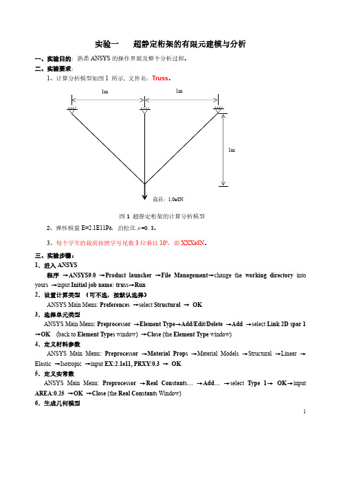
- 1、下载文档前请自行甄别文档内容的完整性,平台不提供额外的编辑、内容补充、找答案等附加服务。
- 2、"仅部分预览"的文档,不可在线预览部分如存在完整性等问题,可反馈申请退款(可完整预览的文档不适用该条件!)。
- 3、如文档侵犯您的权益,请联系客服反馈,我们会尽快为您处理(人工客服工作时间:9:00-18:30)。
三点弯曲计算报告书
2011.3.20
1.算例说明:
三点弯曲实验是材料性能测试中常采用的一种方法,通过该方法可以方便的获得材料的弯曲强度和弯曲模量。
算例试样尺寸参考了实际实验采用的尺寸,试样的支撑及加载方式如图1所示,图2给出了试样的尺寸信息。
图1 三点弯曲示意图
图2 试样尺寸信息
2. 问题分析:
材料特性为各向同性的简支梁,其弯曲应力存在理论解,根据材料力学相关理论[1]。
对于三点弯曲,各截面的应力可以通过公式(*)算出,最大拉压应力出现在集中力作用截面处 。
z I My =σ (*)
式中M 表示弯矩,y 表示截面上点到杆件中性面的距离, z I 表示截面对中性轴的惯性矩。
根据公式(*)可以方便的计算出最大应力值:
MPa I y M m m I m m
h y m m N FL M z
z 76.1188022/4.47504
max max max 4
max max =====⋅==σ
3. 问题求解
从图1中可以看出试样的支撑形式属于简支梁,载荷为单点集中力,据此得到计算用模型及约束和载荷方式。
图4 给出了有限元网格划分。
关材料属性信息:
弹性模量 Elastic Modulus=3.3Gpa
泊松比Poisson ratio=0.3
图3 试样的有限元模型
4.结果分析:
应力分布见图4所示,从图中可以看出,计算结果与理论分析一致,最大应力发生在集中力作用的截面处,有限元计算结果与理论解完全相同。
图4 三点弯曲应力分布图(上图为等轴视图下图为前视图)
参考文献
[1]范钦珊,殷雅俊,虞建伟 . 材料力学(第2版), 清华大学出版社, 2008, P109。