L04_Femur_Shaft_ST_Fx

合集下载

LTE信令流程详解

L T E信令流程详解集团标准化工作小组 #Q8QGGQT-GX8G08Q8-GNQGJ8-MHHGN#LTE信令流程目录概述本文通过对重要概念的阐述，为信令流程的解析做铺垫，随后讲解LTE中重要信令流程，让大家熟悉各个物理过程是如何实现的，其次通过异常信令的解读让大家增强对异常信令流程的判断，再次对系统消息的解析，让大家了解系统消息的特点和携带的内容。

最后通过实测信令内容讲解，说明消息的重要信元字段。

第一章协议层与概念1.1控制面与用户面在无线通信系统中，负责传送和处理用户数据流工作的协议称为用户面；负责传送和处理系统协调信令的协议称为控制面。

用户面如同负责搬运的码头工人，控制面就相当于指挥员，当两个层面不分离时，自己既负责搬运又负责指挥，这种情况不利于大货物处理，因此分工独立后，办事效率可成倍提升，在LTE网络中，用户面和控制面已明确分离开。

1.2接口与协议接口是指不同网元之间的信息交互时的节点，每个接口含有不同的协议，同一接口的网元之间使用相互明白的语言进行信息交互，称为接口协议，接口协议的架构称为协议栈。

在LTE中有空中接口和地面接口，相应也有对应的协议和协议栈。

信令流数据流图1 子层、协议栈与流图2 子层运行方式LTE系统的数据处理过程被分解成不同的协议层。

简单分为三层结构：物理层、数据链路层L2和网络层。

图1阐述了LTE系统传输的总体协议架构以及用户面和控制面数据信息的路径和流向。

用户数据流和信令流以IP包的形式进行传送，在空中接口传送之前，IP包将通过多个协议层实体进行处理，到达eNodeB后，经过协议层逆向处理，再通过S1/X2接口分别流向不同的EPS实体，路径中各协议子层特点和功能如下：1.2.1NAS协议（非接入层协议）处理UE和MME之间信息的传输，传输的内容可以是用户信息或控制信息（如业务的建立、释放或者移动性管理信息）。

它与接入信息无关，只是通过接入层的信令交互，在UE和MME之间建立起了信令通路，从而便能进行非接入层信令流程了。

Matrox Meteor-II Pulnix TM-4000CL摄像头接口应用说明书

Exposure time: The width (falling edge to rising edge) of the EXPOSURE1 (CC1) signal is the exposure time. The exposure time can be modified using Matrox Intellicam or with the MIL MdigControl() function. Refer to the respective manual for more information.
signal to camera to initiate and control exposure time. Matrox Meteor-II/Camera Link receiving LDV, FDV, CLK and video signal
from camera. x2048Pcon.DCF
Camera control settings: AccuPiXEL Dual-Tap camera control software version 2.0 or higher can be used.
Control
Setting
Shutter Mode ASYNC (external pulse width)
parentheses as per camera manufacturer)
Basics about the interface modes
Camera Descriptions
Effective resolution: 2048 × 2048 × 8-bit @ 15 fps. Camera Link BASE interface (Dual tap). Progressive scan. Internal sync. Internal or external exposure control. 40 MHz pixel clock rate.

四旋翼基础算法学习2-IMU输入滤波算法

IMU采集频率：Crazepony 100Hz（10ms），匿名小四 1000Hz（1ms），圆点博士小四333Hz（3ms）。本次测试使用 250Hz（4ms）。
在从传感器读取的原始数据滤波之前，一般需要进行零偏校准。一般陀螺仪需要上电校准零偏，加计的零偏与IMU安装有关，校准一次以后上电始终使用校准值即可（或者不予校准）。零偏校准方法基本都是水平静止放置机体多次采样取均值。
GYRO_Y 滤波后加速度x轴数据
GYRO_Z 滤波后加速度z轴数据
1.加速度计滑动均值滤波
代码：
#define SAF_NUM 10 void Slide_Average_Filter(int16_t acc_x,int16_t acc_y,int16_t acc_z,int16_t *acc_out_x,int16_t *acc_out_y,int16_t *acc_out_z) {
for(cnt=0;cnt<SAF_NUM;cnt++) {
temp1 += filter_buffer[0][cnt]; temp2 += filter_buffer[1][cnt]; temp3 += filter_buffer[2][cnt]; } *acc_out_x = temp1/SAF_NUM; *acc_out_y = temp2/SAF_NUM; *acc_out_z = temp3/SAF_NUM;
博客园用户登录代码改变世界密码登录短信登录忘记登录用户名忘记密码记住我登录第三方登录/注册没有账户, 立即注册
四旋翼基础算法学习 2-IMU输入滤波算法
前言：
处理器读取陀螺仪加速度计数据后首先需要对数据进行滤波处理，此文分析比较几种常用的滤波算法。

Flux estimator of the 3-ph induction motor

ACI_FE Flux estimator of the 3-ph induction motorDescriptionThis software module implements the flux estimator with the rotor flux angle for the 3-phinduction motor based upon the integral of back emf’s (voltage model) approach. Toreduce the errors due to pure integrator and stator resistance measurement, thecompensated voltages produced by PI compensators are introduced. Therefore, this fluxestimator can be operating over a wide range of speed, even at very low speed.Module VariablesFormatRange Name DescriptionInputsu_ds_fe Stationary d-axis stator voltage (pu) Q15 -1 -> 0.999u_qs_fe Stationary q-axis stator voltage (pu) Q15 -1 -> 0.999i_ds_fe Stationary d-axis stator current (pu) Q15 -1 -> 0.999i_qs_fe Stationary q-axis stator current (pu) Q15 -1 -> 0.999Outputspsi_dr_fe Stationary d-axis rotor flux linkage (pu) Q15 -1 -> 0.999psi_qr_fe Stationary q-axis rotor flux linkage (pu)Q15 -1 -> 0.999theta_r_fe Rotor flux linkage angle (pu) Q15 -1 -> 0.999Init / Config These constants are computed basing on themachine parameters (Rs, Ls, Lr, Lm, Tr), basequantities (Ib, Vb), and sampling period (T).K1 K1 = Tr/(Tr+T) Q15 -1 -> 0.999K2 K2 = T/(Tr+T)Q15 -1 -> 0.999K3 K3 = Lm/Lr Q15 -1 -> 0.999K4 K4 = (Ls*Lr-Lm*Lm)/(Lr*Lm) Q15 -1 -> 0.999K5 K5 = Rs*Ib/Vb Q15 -1 -> 0.999K6 K6 = T*Vb/(Lm*Ib) Q15 -1 -> 0.999K7 K7 = Lr/Lm Q14 -2 -> 1.999K8 K8 = (Ls*Lr-Lm*Lm)/(Lm*Lm) Q15 -1 -> 0.999Module StatisticsAssembly Filename:aci_fe.asmASM Routines: ACI_FE, ACI_FE_INITParameter calculation excel file:aci_fe_init.xlsC-callable ASM filename(s): aci_fe.asm, aci_fe.hType:: Target Independent, Application DependentTarget Device/s:x24x / x24xxItem Asm only C callable ASM Comments Code size 286 words 306 words1Data RAM 46 words 0 words1xDAIS module No NoxDAIS component No NoMultiple Instances No Yes1 Each pre-initialized ACIFE structure instance consumes 37 words in the .cinit section and 35 words in data memory.Module Usage / Calling ConventionASM onlyRoutine names and calling limitation:There are two routines involved:ACI_FE, the main routine; andACI_FE_INIT, the initialization routine.The initialization routine must be called during program initialization. The ACI_FE routine must be called in the control loop.Variable Declaration:In the system file, including the following statements before calling the subroutines:FunctioncallsACI_FE_INIT ;ACI_FE,.ref.ref psi_dr_fe, psi_qr_fe, theta_r_fe ; OutputsInputsi_qs_fe ;i_ds_fe,.ref;Inputsu_ds_fe,.refu_qs_feMemory map:All variables are mapped to an uninitialized named section, fe_aci, which can be allocated to any one data page.Example code:During system initialization specify the ACI_FE parameters as follows:LDP #K1_feSPLK #K1_fe_,K1_fe ; K1 = Tr/(Tr+T) (Q15)SPLK #K2_fe_,K2_fe ; K2 = T(Tr+T) (Q15)SPLK #K3_fe_,K3_fe ; K3 = Lm/Lr (Q15)SPLK #K4_fe_,K4_fe ; K4 = (Ls*Lr-Lm*Lm)/(Lr*Lm) (Q15)SPLK #K5_fe_,K5_fe ; K5 = Rs*Ib/Vb (Q15)SPLK #K6_fe_,K6_fe ; K6 = T*Vb/(Lm*Ib) (Q15)SPLK #K7_fe_,K7_fe ; K7 = Lr/Lm (Q14)SPLK #K8_fe_,K8_fe ; K8 = (Ls*Lr-Lm*Lm)/(Lm*Lm) (Q15)Then in the interrupt service routine call the module and read results as follows:LDP #u_ds_fe ; Set DP for module inputsBLDD #input_var1,u_ds_fe ; Pass input variables to module inputsBLDD #input_var2,u_qs_fe ; Pass input variables to module inputsBLDD #input_var3,i_ds_fe ; Pass input variables to module inputsBLDD #input_var4,i_qs_fe ; Pass input variables to module inputsCALL ACI_FEmoduleoutputforDPSetLDP #output_var1 ;BLDD #psi_dr_fe,output_var1 ; Pass output to other variablesBLDD #psi_qr_fe,output_var2 ; Pass output to other variablesBLDD #theta_r_fe,output_var3 ; Pass output to other variablesC/C-callable ASM onlyObject DefinitionThe structure of the ACIFE object is defined in the header file, aci_fe.h, as seen in the following:typedef struct { int theta_r_fe; /* Output: Rotor flux angle (Q15) */int i_qs_fe; /* Input: Stationary q-axis stator current (Q15) */int i_ds_fe; /* Input: Stationary d-axis stator current (Q15) */int K1_fe; /* Parameter: Constant using in current model (Q15) */int flx_dr_e /* Variable: Rotating d-axis rotor flux (current model) (Q15) */int K2_fe; /* Parameter: Constant using in current model (Q15) */int flx_qr_s; /* Variable: Stationary q-axis rotor flux (current model) (Q15) */int flx_dr_s; /* Variable: Stationary d-axis rotor flux (current model) (Q15) */int K3_fe; /* Parameter: Constant using in stator flux computation (Q15) */int K4_fe; /* Parameter: Constant using in stator flux computation (Q15) */int flx_ds_s; /* Variable: Stationary d-axis stator flux (current model) (Q15) */int flx_qs_s; /* Variable: Stationary q-axis stator flux (current model) (Q15) */ int psi_ds_fe; /* Variable:Stationary d-axis stator flux (voltage model) (Q31) */ int Kp_fe; /* Parameter: PI proportionnal gain (Q15) */int ui_lo_ds; /* Variable: Stationary d-axis integral term (Q30) */int ui_hi_ds; /* Variable: Stationary d-axis integral term (Q30) */int ucomp_ds; /* Variable: Stationary d-axis compensated voltage (Q15) */int Ki_fe; /* Parameter: PI integral gain (Q31-16bit) */int psi_qs_fe; /* Variable: Stationary q-axis stator flux (voltage model) (Q31) */int ui_lo_qs; /* Variable: Stationary q-axis integral term (Q30) */int ui_hi_qs; /* Variable: Stationary q-axis integral term (Q30) */int ucomp_qs; /* Variable: Stationary q-axis compensated voltage (Q15) */int emf_ds /* Variable: Stationary d-axis back emf (Q15) */int u_ds_fe; /* Input: Stationary d-axis stator voltage (Q15) */int K5_fe; /* Parameter: Constant using in back emf computation (Q15) */int K6_fe; /* Parameter: Constant using in back emf computation (Q15) */int psi_ds_lo; /* Variable: Stationary d-axis stator flux (voltage model) (Q31) */int emf_qs /* Variable: Stationary q-axis back emf (Q15) */int u_qs_fe; /* Input: Stationary q-axis stator voltage (Q15) */int psi_qs_lo; /* Variable: Stationary q-axis stator flux (voltage model) (Q31) */int K8_fe; /* Parameter: Constant using in rotor flux computation (Q15) */int K7_fe; /* Parameter: Constant using in rotor flux computation (Q14) */int psi_dr_fe; /* Output: Stationary d-axis estimated rotor flux (Q15) */int psi_qr_fe; /* Output: Stationary q-axis estimated rotor flux (Q15) */int (*calc)(); /* Pointer to calculation function */} ACIFE;Special Constants and Data typesACIFE The module definition itself is created as a data type. Thismakes it convenient to instance a ACIFE object. To createmultiple instances of the module simply declare variables oftype ACIFE.ACIFE_DEFAULTS Initializer for the ACIFE object. This provides the initial valuesto the terminal variables, internal variables, as well as methodpointers. This is initialized in the header file,aci_fe.h. Methodsvoid aci_fe_calc(ACIFE *);This default definition of the object implements just one method – the runtime compute function for flux and its angle estimator. This is implemented by means of a function pointer, and the default initializer sets this to aci_fe_calc function. The argument to this function is the address of the ACIFE object. Again, this statement is written in the header file, aci_fe.h.Module UsageInstantiationThe following example instances two such objects:ACIFE fe1, fe2;InitializationTo instance a pre-initialized object:ACIFE fe1 = ACIFE_DEFAULTS;ACIFE fe2 = ACIFE_DEFAULTS;Invoking the compute functionfe1.calc(&fe1);fe2.calc(&fe2);ExampleLets instance two ACIFE objects, otherwise identical, and compute two flux estimators. The following example is the c source code for the system file.ACIFE fe1= ACIFE_DEFAULTS; /* instance the first object */ACIFE fe2= ACIFE_DEFAULTS; /* instance the second object */main(){fe1.u_ds_fe= voltage_dq1.d; /* Pass inputs to fe1 */fe1.u_qs_fe= voltage_dq1.q; /* Pass inputs to fe1 */fe1.i_ds_fe=current_dq1.d; /* Pass inputs to fe1 */fe1.i_qs_fe=current_dq1.q; /* Pass inputs to fe1 */fe2.u_ds_fe= voltage_dq2.d; /* Pass inputs to fe2 */fe2.u_qs_fe= voltage_dq2.q; /* Pass inputs to fe2 */fe2.i_ds_fe=current_dq2.d; /* Pass inputs to fe2 */fe2.i_qs_fe=current_dq2.q; /* Pass inputs to fe2 */}void interrupt periodic_interrupt_isr(){fe1for*/function fe1.calc(&fe1); /*Callcomputefe2*/forcomputefe2.calc(&fe2); /*Callfunctionflux1.d = fe1.psi_dr_fe; /* Access the outputs of fe1 */flux1.q = fe1.psi_qr_fe; /* Access the outputs of fe1 */angle1 = fe1.theta_r_fe; /* Access the outputs of fe1 */flux2.d = fe2.psi_dr_fe; /* Access the outputs of fe2 */flux2.q = fe2.psi_qr_fe; /* Access the outputs of fe2 */angle2 = fe2.theta_r_fe; /* Access the outputs of fe2 */}Technical Background:The overall of the flux estimator [1] can be shown in Figure 1. The rotor flux linkages in the stationary reference frame are mainly computed by means of the integral of back emf’s in the voltage model. By introducing the compensated voltages generated by PI compensators, the errors associated with pure integrator and stator resistance measurement can be taken care. The equations derived for this flux estimator are summarized as follows:Continuous time:Firstly, the rotor flux linkage dynamics in synchronously rotating reference frame ()r e ψω=ω=ω can be shown as below:()i ,e qr r e i ,e dr re ds r m i ,e dr1i L dt d ψω−ω+ψτ−τ=ψ (1)()i,e dr r e i ,e qr re qs r m i,e qr1i L dt d ψω−ω−ψτ−τ=ψ (2)where L m is the magnetizing inductance (H), rr r R L=τis the rotor time constant (sec), andωr is the electrically angular velocity of rotor (rad/sec).In the current model, total rotor flux linkage is aligned into the d-axis component, which is modeled by the stator currents, thusi ,e dr i ,e r ψ=ψ and 0i,e qr =ψ(3) Substituting 0i,e qr =ψ into (1)-(2), yields the oriented rotor flux dynamics are i,e dr re ds r m i,e dr 1i L dt d ψτ−τ=ψ (4)0i,e qr =ψ(5) Note that (4) and (5) are the classical rotor flux vector control equations. Then, the rotor flux linkages in (4)-(5) are transformed into the stationary reference frame performed by inverse park transformation.()()()r r r cos sin cos i,e dr i ,e qr i ,e dr i ,s dr ψψψθψ=θψ−θψ=ψ(6)()()()r r r sin cos sin i,e dr i ,e qr i ,e dr i ,s qr ψψψθψ=θψ+θψ=ψ(7)where r ψθis the rotor flux angle (rad).Then, the stator flux linkages in stationary reference frame are computed from the rotor flux linkages in (6)-(7)i,s dr r m s ds r 2m r s s drm s dss i,s dsL L i L L L L i L i L ψ+⎟⎟⎠⎞⎜⎜⎝⎛−=+=ψ (8) i ,s qr r m s qs r 2m r s sqr m s qs s i ,s qs L L i L L L L i L i L ψ+⎟⎟⎠⎞⎜⎜⎝⎛−=+=ψ (9) where L s and L r are the stator and rotor self inductance (H), respectively.Next, the stator flux linkages in the voltage model is computed by means of back emf’s integration with compensated voltages.()d t u R i u ds ,comp s sds s ds v ,s ds ∫−−=ψ(10) ()d t u R i u qs,comp s s qs s qs v,s qs∫−−=ψ(11)where R s is the stator resistance (Ω), sqs s ds u ,u are stationary dq-axis stator voltages, andthe compensated voltages are computed by the PI control law as follows:()()d t T K K u i,s ds v ,s ds Ipi ,s ds v ,s ds p ds ,comp ∫ψ−ψ+ψ−ψ= (12) ()()d t T K K u i ,s qs v ,s qs IP i ,s qs v ,s qs p qs ,comp ∫ψ−ψ+ψ−ψ= (13) The proportional gain K P and the reset time T I are chosen such that the flux linkages computed by current model is dominant at low speed because the back emf’s computed by the voltage model are extremely low at this speed range (even zero back emf’s at zero speed). While at high speed range, the flux linkages computed by voltage model is dominant.Once the stator flux linkages in (10)-(11) are calculated, the rotor flux linkages based on the voltage model are further computed, by rearranging (8)-(9), asv,s ds m r s ds m 2m r s v ,s dr L L i L L L L ψ+⎟⎟⎠⎞⎜⎜⎝⎛−−=ψ (14) v ,s qs m r s qs m 2m r s v ,s qrL L i L L L L ψ+⎟⎟⎠⎞⎜⎜⎝⎛−−=ψ (15) Then, the rotor flux angle based on the voltage model is finally computed as⎟⎟⎠⎞⎜⎜⎝⎛ψψ=θ−ψv ,s dr v,s qr 1tanr (16) Discrete time:The oriented rotor flux dynamics in (4) is discretized by using backward approximation as follows:e,i e,ie e,i dr dr m dsdr r r(k)(k 1)L 1i (k)(k)T ψ−ψ−=−ψττ (17) where T is the sampling period (sec). Rearranging (17), then it givese,i e,i er m drdr ds r r L T (k)(k 1)i (k)T T ⎛⎞⎛⎞τψ=ψ−+⎜⎟⎜⎟τ+τ+⎝⎠⎝⎠(18) Next, the stator flux linkages in (10)-(11) are discretized by using trapezoidal (or tustin) approximation as())1k (e )k (e 2T )1k ()k (s ds s ds v,s ds v ,s ds −++−ψ=ψ(19) ())1k (e )k (e 2T )1k ()k (s qs s qs v,s qs v ,s qs −++−ψ=ψ(20) where the back emf’s are computed as)k (u R )k (i )k (u )k (e ds ,comp s sds s ds s ds −−=(21) )k (u R )k (i )k (u )k (e qs ,comp s sqs s qs s qs −−=(22)Similarly, the PI control laws in (12)-(13) are also discretized by using trapezoidal approximation as())1k (u )k ()k (K )k (u i ,ds ,comp i,s ds v ,s ds p ds ,comp −+ψ−ψ=(23) ())1k (u )k ()k (K )k (u i ,qs ,comp i,s qs v ,s qs p qs ,comp −+ψ−ψ=(24)where the accumulating integral terms are as()())k ()k (K K )1k (u )k ()k (T T K )1k (u )k (u i,s ds v ,s ds I P i ,ds ,comp i,s ds v ,s ds I P i ,ds ,comp i ,ds ,comp ψ−ψ+−=ψ−ψ+−=(25)()())k ()k (K K )1k (u )k ()k (TTK )1k (u )k (u i,s qs v ,s qs I P i ,qs ,comp i,s qsv ,s qs IP i,qs ,comp i ,qs ,comp ψ−ψ+−=ψ−ψ+−= (26)where II T TK =.Discrete time and Per-unit:Now all equations are normalized into the per-unit by the specified base quantities. Firstly, the rotor flux linkage in current model (18) is normalized by dividing the base flux linkage ase,i e,i er dr,pudr,pu ds,pu r r T (k)(k 1)i (k)T T ⎛⎞⎛⎞τψ=ψ−+⎜⎟⎜⎟τ+τ+⎝⎠⎝⎠ pu (27) where b m b I L =ψ is the base flux linkage (volt.sec) and I b is the base current (amp).Next, the stator flux linkages in the current model (8)-(9) are similarly normalized by dividing the base flux linkage as)k (L L )k (i L L L L L )k (i ,s pu ,dr r m s pu ,ds m r 2m r s i,s pu ,ds ψ+⎟⎟⎠⎞⎜⎜⎝⎛−=ψ pu (28))k (L L )k (i L L L L L )k (i,s pu ,qr r m s pu ,qs m r 2m r s i,s pu,qs ψ+⎟⎟⎠⎞⎜⎜⎝⎛−=ψ pu (29) Then, the back emf’s in (21)-(22) are normalized by dividing the base phase voltage V b)k (u )k (i V R I )k (u )k (e pu ,ds ,comp s pu ,ds bs b spu,ds s pu ,ds −−= pu (30) )k (u )k (i V R I )k (u )k (e pu ,qs ,comp s pu ,qs bs b spu,qs s pu ,qs −−= pu (31) Next, the stator flux linkages in the voltage model (19)-(20) are divided by the base flux linkage.⎟⎟⎠⎞⎜⎜⎝⎛−++−ψ=ψ2)1k (e )k (e I L T V )1k ()k (spu ,ds s pu ,ds b m b v ,s pu ,ds v ,s pu ,ds pu (32) ⎟⎟⎠⎞⎜⎜⎝⎛−++−ψ=ψ2)1k (e )k (e I L T V )1k ()k (spu ,qs s pu ,qs b m b v ,s pu ,qs v ,s pu ,qs pu (33) Similar to (28)-(29), the normalized rotor flux linkages in voltage model are)k (L L )k (i L L L L L )k (v,s pu ,ds m r s pu ,ds m m 2m r s v ,s pu ,dr ψ+⎟⎟⎠⎞⎜⎜⎝⎛−−=ψ pu (34) )k (L L )k (i L L L L L )k (v,s pu ,qs m r s pu ,qs m m 2m r s v ,s pu,qr ψ+⎟⎟⎠⎞⎜⎜⎝⎛−−=ψ pu (35) In conclusion, the discrete-time, per-unit equations are rewritten in terms of constants.Current model – rotor flux linkage in synchronously rotating reference frame ()rψω=ωe,i e,i edr,pu 1dr,pu 2ds,pu (k)K (k 1)K i (k)ψ=ψ−+ pu(36)where T K r r 1+ττ=, and TTK r 2+τ=. Current model – rotor flux linkages in the stationary reference frame ()0=ω)k (K )k (i K )k (i,s pu ,dr 3s pu ,ds 4i ,s pu ,ds ψ+=ψ pu(37) )k (K )k (i K )k (i ,s pu ,qr 3s pu ,qs 4i ,s pu ,qs ψ+=ψ pu(38)where r m3L L K =, and mr 2m r s 4L L L L L K −=. Voltage model – back emf’s in the stationary reference frame ()0=ω)k (u )k (i K )k (u )k (e pu ,ds ,comp spu ,ds 5s pu ,ds s pu ,ds −−= pu(39))k (u )k (i K )k (u )k (e pu ,qs ,comp s pu ,qs 5s pu ,qs s pu ,qs −−= pu (40)where bsb 5V R I K =. Voltage model – stator flux linkages in the stationary reference frame ()0=ω⎟⎟⎠⎞⎜⎜⎝⎛−++−ψ=ψ2)1k (e )k (e K )1k ()k (spu ,ds s pu ,ds 6v ,s pu,ds v,s pu,ds pu (41) ⎟⎟⎠⎞⎜⎜⎝⎛−++−ψ=ψ2)1k (e )k (e K )1k ()k (spu ,qs s pu ,qs 6v ,s pu ,qs v ,s pu ,qs pu (42) where bm b 6I L TV K =.Voltage model – rotor flux linkages in the stationary reference frame ()0=ω)k (K )k (i K )k (v,s pu ,ds 7s pu ,ds 8v ,s pu ,dr ψ+−=ψ pu(43) )k (K )k (i K )k (v,s pu ,qs 7s pu ,qs 8v ,s pu ,qr ψ+−=ψ pu(44)where m r7L L K =, and mm 2m r s 8L L L L L K −=. Voltage model – rotor flux angle⎟⎟⎠⎞⎜⎜⎝⎛ψψπ=θ−ψ)k ()k (tan 21)k (v ,s pu ,dr v ,s pu ,qr 1pu ,r pu (45) Notice that the rotor flux angle is computed by a look-up table of 0o -45o with 256 entries.In fact, equations (36)-(44) are mainly employed to compute the estimated flux linkages in per-unit. The excel file aci_fe_init.xls is used to compute these eight constants (i.e., K 1,…,K 8) in the appropriately defined Q system. This file can directly compute the hexadecimal/decimal values of these K’s in order to put them into the ACI_FE_INIT module easily. The required parameters for this module are summarized as follows:The machine parameters: - stator resistance (R s ) - rotor resistance (R r )- stator leakage inductance (L sl ) - rotor leakage inductance (L rl ) - magnetizing inductance (L m )The based quantities: - base current (I b )- base phase voltage (V b )The sampling period: - sampling period (T)Notice that the stator self inductance is m sl s L L L += (H) and the rotor self inductance is m rl r L L L +=(H).Next, Table 1 shows the correspondence of notations between variables used here and variables used in the program (i.e., aci_fe.asm). The software module requires that both input and output variables are in per unit values (i.e., they are defined in Q15).Table 1: Correspondence of notationsReferences:[1] C. Lascu, I. Boldea, and F. Blaabjerg, “A modified direct torque control for inductionmotor sensorless drive”, IEEE Trans. Ind. Appl., vol. 36, no. 1, pp. 122-130, January/February 2000.。

EFLOW用户指南 Release 12.3说明书

NVIDIA-provided CUDA containers from the NGC registry can be deployed directly. If you are preparing a CUDA docker container, ensure that the necessary toolchains are installed.
Path
:
Online
: True
RestartNeeded : False
2. Set execution policy and verify.
Set-ExecutionPolicy -ExecutionPolicy AllSigned -Force
Get-ExecutionPolicy AllSigned
5
EFLOW User's Guide, Release 12.3
3. Download and install EFLOW.
$msiPath = $([io.Path]::Combine($env:TEMP, 'AzureIoTEdge.msi')) $ProgressPreference = 'SilentlyContinue' Invoke-WebRequest "https:∕∕aka.ms∕AzEFLOWMSI_1_4_LTS_X64" -OutFile $msiPath
▶ The Windows host OS with virtualization enabled ▶ A Linux virtual machine ▶ IoT Edge Runtime ▶ IoT Edge Modules, or otherwise any docker-compatible containerized application (runs on

_NCCP1H010_MoveAbsolute_REAL

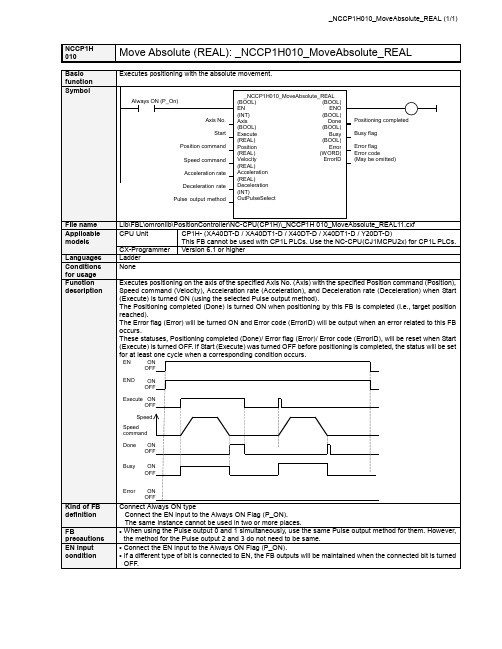
NCCP1HMove Absolute (REAL): _NCCP1H010_MoveAbsolute_REAL 010■ Variable TableOutput Variables Name Variable name Data type Range DescriptionENO ENO BOOL 1(ON): FB operating normally0(OFF): FB not operating normallyPositioning completed Done BOOL 1 (ON) indicates that positioning is completed.Busy flag Busy BOOL 1 (ON) indicates that the FB is in pregress.Error flag Error BOOL 1 (ON) indicates that an error has occurred in the FB. Error code(May be omitted)ErrorIDWORDThe error code of the error occurred in the FB will be output. For details of the errors, refer to the sections of the manual listed in the Related manuals above. When Unit No. or Axis. No. is out of the range, #0000 will be output.Limitation of Function block by Combination of CPU type and Unit Version CPU Type Unit Version Axis No. Range of Frequency Description 1.1 &0 to &3 +1.0 to +100000.0 &0 to &1 +1.0 to +100000.0XA / X 1.0 &2 to &3 +1.0 to +30000.0Please use Function Block Version1.10 or higher whenyou set values that are larger than 30000.0Hz to Axis. No.2 or No.3. &0 to &1 +1.0 to +1000000.0 Y 1.1 &2 to &3 +1.0 to +100000.0Please use Function Block Version1.10 or higher forCP1H-Y20DT-D.■ Revision History Version Date Contents 1.10 2006.5. Addition of CP1H CPU Unit unit version 1.1 1.00 2005.9. Original productionNoteThis document explains the function of the function block.It does not provide information of restrictions on the use of Units and Components or combination of them. For actual applications, make sure to read the operation manuals of the applicable products.。

The absorption spectrum of V838 Mon in 2002 February - March. I. Atmospheric parameters and

a r X i v :a s t r o -p h /0411032v 1 1 N o v 2004Mon.Not.R.Astron.Soc.000,1–7(2004)Printed 2February 2008(MN L A T E X style ﬁle v2.2)The absorption spectrum of V838Mon in 2002February -March.I.Atmospheric parameters and iron abundance.⋆Bogdan M.Kaminsky 1†,Yakiv V.Pavlenko 1‡1Main Astronomical Observatory of Ukrainian Academy of Sciences,Golosiiv woods,03680Kyiv-127,UkraineReceived ;acceptedABSTRACTWe present a determination of the eﬀective temperatures,iron abundances,and mi-croturbulent velocities for the pseudophotosphere of V838Mon on 2002February 25,and March 2and 26.Physical parameters of the line forming region were obtained in the framework of a self-consistent approach,using ﬁts of synthetic spectra to observed spectra in the wavelength range 5500-6700˚A .We obtained T eﬀ=5330±300K,5540±270K and 4960±190K,for February 25,March 2,and March 26,respectively.The iron abundance log N (Fe)=−4.7does not appear to change in the atmosphere of V838Mon from February 25to March 26,2002.Key words:stars:atmospheres –stars:abundances –stars:individual:V838Mon1INTRODUCTIONThe peculiar variable star V838Mon was discovered during an outburst in the beginning of 2002January (Brown 2002).Two further outbursts were then observed in 2002February (Munari et al.2002a;Kimeswenger et al.2002;Crause et al.2003)and in general the optical brightness in V-band of the star increased by 9mag.Since 2002March,a gradual fall in V-magnitude began which,by 2003January,was re-duced by 8mag.The suspected progenitor of V838Mon was identiﬁed by Munari et al.(2002a)as a 15mag F-star on the main sequence.Possibly V838Mon might have a B3V companion (Desidera &Munari 2002),but it could be a background star.The discovery of a light echo (Henden et al.2002)allowed an estimate of the distance to V838Mon and,according to recent works based on HST data (Bond et al.2003;Tylenda 2004)its distance is 5-6kpc.If these estimations are correct,at the time of maximum brightness V838Mon was the most luminous star in our Galaxy.Details of the spectral evolution of the star are described in Kolev et al.2002;Wisniewski et al.2003;Osiwala et al.2002).During outbursts (except for the last)the spec-trum displayed numerous emission lines with P Cyg pro-ﬁles,formed in the expanding shell and around an F-or A-star (Kolev et al.2002).On the other hand,absorption spectra appropriate to a red giant or supergiant were ob-served in quiescent periods.Strong lines of hydrogen,D lines of sodium,triplets of calcium and other elements show P⋆Based in part on observations collected with the 1.83m tele-scope of the Astronomical Observatory in Asiago,Italy †E-mail:bogdan@mao.kiev.ua ‡E-mail:yp@mao.kiev.uaCyg proﬁles.They have similar proﬁles and velocities vary-ing from −500km s −1in late January to −280km s −1in late March (Munari et al.2002a).Since the middle of 2002March,the emissions are considerably weakened and the spectrum of V838Mon evolved to later spectral classes.In middle of 2002April,there were present some lines of TiO;in May the spectrum evolved to the“very cold”M-giant (Banerjee &Ashok 2002).In October Evans et al.(2003)characterized it as a L-supergiant.Recently Kipper et al.(2004)found for iron group ele-ments [m/H]=−0.4,while abundances of lithium and some s-process elements are clearly enhanced.This results was obtain using the static LTE model.These results are very dependent on the model atmo-sphere and spectrum synthesis assumptions.The nature of the outbursts remains a mystery.Possible explanations include various thermonuclear processes (very slow nova,ﬂare post-AGB),and the collision of two stars (Soker &Tylenda 2003).Munari et al.(2002a)suggested that V838Mon is a new type of a variable star,because comparison with the closely analogous V4334Sgr and M31RV has shown signiﬁcant enough diﬀerences in the observed parameters.In this paper we discuss the results of the determina-tion of iron abundance and atmospheric parameters of V838Mon.These we obtained from an analysis of absorption spec-tra of V838Mon on 2002February 25and March 2and 26.The complexity and uniqueness of the observed character-istics of V838Mon practically excluded a deﬁnition of the parameters of the atmosphere using conventional methods,based on calibration on photometric indices,ionization bal-ance,proﬁles of hydrogen lines.Indeed,the presence around the star of a dust shell,and the uncertain determination of2Bogdan M.Kaminsky,Yakiv V.Pavlenko interstellar reddening(from E B−V=−0.25to E B−V=−0.8 Munari et al.2002a),aﬀects the U−B and B−V colours. Emission in the hydrogen lines provides severe problems for their application in the estimation of eﬀective temperature. Moreover,both the macroturbulent motions and expansion of the pseudophotosphere merges the numerous lines in wide blends.As a result,a single unblended line in the spectrum of V838Mon cannot be found at all,and any analysis based on measurements of equivalent widths is completely excluded.The observational data used in this paper are described in section2.Section3explains some background to our work and some details of the procedure used.We attempt to de-termine T eﬀ,the microturbulent velocity V t and the iron abundance log N(Fe)in the atmosphere of V838Mon in theframework of the self-consistent approach in section4.Some results are discussed in section5.2OBSER V ATIONSSpectra of V838Mon were obtained on2002February25 and March26with the Echelle+CCD spectrograph on the 1.82m telescope operated by Osservatorio Astronomico di Padova on Mount Ekar(Asiago),and freely available to the community from http://ulisse.pd.astro.it/V838Mon/.A 2arcsec slit was used withﬁxed E-W orientation,produc-ing a PSF with a FWHM of1.75pixels,corresponding to a resolving power close to20000.The detector was a UV coated Thompson CCD1024×1024pixel,19micron square size,covering in one exposure the wavelength range4500to 9480˚A(echelle orders#49to#24).The short wavelength limit is set by a2mm OG455long-passﬁlter,inserted in the optical train to cut the second order from the cross-disperser. The wavelength range is covered without gaps between ad-jacent echelle orders up to7300˚A.The spectra have been extracted and calibrated using IRAF software running un-der Linux operating system.The spectra are sky-subtracted andﬂat-ﬁelded.The wavelength solution was derived simul-taneously for all26echelle orders,with an average r.m.s of 0.18km s−1.The8480-8750˚A wavelength range of these Asi-ago spectra has been described in Munari et al.(2002a,b).Another set of spectra(R∼32000)for March2was obtained with the echelleﬁbre-fed spectrograph on the1.9-m SAAO telescope kindly provided for us by Dr.Lisa Crause (see Crause et al.2003for details).3PROCEDURETo carry out our analysis of V838Mon we used the spectral synthesis techniques.Our synthetic spectra were computed in the framework of the classical approach:LTE,plane-parallel media,no sinks and sources of energy inside the atmosphere,and transfer of energy provided by the radia-tionﬁeld and by convection.Strictly speaking,none of these assumptions is100% valid in atmosphere of V838Mon.Clearly we have non-static atmosphere which may well have shock waves mov-ing trough it.Still we assumed that in any moment the structure of model atmosphere of V838Mon is similar to model atmospheres of supergiants.Indeed,temporal changes of the absorption spectra on the days were rather marginal.0.00050.0010.00150.0020.00250.0030.00350.004-200-150-100-50 0 50 100 150 200Velocity (km s-1)V exp=160 km s-1V*sin i=80 km s-1V macro=50 km s-1parison of expansion(V exp=160km s−1),rota-tional(v∗sin i=80km s−1)and macroturbulent(V macro=50 km s−1)proﬁles used in this paper to convolve synthetic spectra.Most probably,for this object,we see only a pseudophoto-sphere,which is the outermost part of an expanding enve-lope.Therefore,ourﬁrst goal was to determine whether it is possible toﬁt our synthetic spectra to the observed V838 Mon spectra.At the time of the observations the spectral class of V838Mon was determined as K-type(Kolev et al.2002). Absorption lines in spectrum of V838Mon form compara-tively broad blends.Generally speaking,there may be a number of broad-ening mechanisms:•Microturbulence,which is formed by small scale(i.e τ≪1)motions in the atmosphere.In the case of a super-giant,V t usualy does not exceed10km s−1.In our analysis we determined V t from a comparison of observed and com-puted spectra.•Stellar rotation.Our analysis shows that,in the case of V838,we should adopt v∗sin i=80km s−1toﬁt the observed spectra.This value is too high for the later stages of stellar evolution,for obvious reasons.In reality rotation cannot contribute much to the broadening of lines observed in spectra of most supergiants.•Expansion of the pseudophotosphere of the star.Asym-metrical proﬁles of expansion broadening can be described, to aﬁrst approximation,by the formulaG(v,λ,∆λ)=const∗∆λThe absorption spectrum of V838Mon3−0.50.511.522.5566056705680569057005710N o r m a l i s e d F l u xWavelength (Å)February 3February 25March 2March 26Figure 2.Spectra of V838Mon observed on February 3,Febru-ary 25,March 2and March 262002emission:many lines are observed in emission.This demon-strates that eﬀects of the radial expansion of the line-forming layers were not signiﬁcant for the dates of our data and for-mally obtained value V exp =160km s −1is not real.•Macroturbulence.After the large increase of luminos-ity in 2002January-February,large scale (i.e.of magnitude τ>1)macroturbulent motions should be very common in the disturbed atmosphere of V838Mon.Our numerical ex-periments showed that,to get appropriate ﬁts to the ob-served spectra taking into account only macroturbulent ve-locities,we should adopt V macro ∼50km s −1.In any case,for the times of our observations the spectra of V838Mon resemble the spectra of “conventional”super-giants.Our V838Mon spectra for February 25,March 2and 26agree,at least qualitatively,with the spectrum of Arcturus (K2III),convolved with macroturbulent velocity proﬁle,given by a gaussian of half-width V macro =50km s −1(Fig.3).The observed emissions in the cores of the strongest lines are formed far outside,perhaps at the outer boundary of the expanding envelope,i.e.in the region which is heated by shock wave dissipation.As result of our ﬁrst numerical experiments,we con-cluded that the spectra of V838Mon in 2002February -March were similar to the spectrum of a normal late (su-per)giant,broadened by strong macroturbulence motions and/or expansion of its pseudophotosphere.Unfortunately we cannot,from the observed spectra,distinguish between broadening due to the macroturbulence and expansion (see next section).It is worth noting that the observed spectra of V838Mon are formed in a medium with decreasing temperature to the outside,i.e.in the local co-moving system of co-ordinates the atmosphere,to a ﬁrst approximation,can be described by a “normal”model,at least in the region of formation of weak or intermediate strength atomic lines.0.10.20.3 0.4 0.5 0.6 0.7 0.8 0.91 1.1 570057105720573057405750N o r m a l i s e d F l u xWavelength (Å)V 838 Mon ArcturusArcturus conv. V macro =50 km s −1Figure parison of the spectrum of V838Mon and that of Arcturus,convolved with macroturbulent proﬁle V macro =50km s −13.1Fits to observed spectraWe computed a sample of LTE synthetic spectra for a grid of Kurucz (1993)model atmospheres with T eﬀ=4000–6000K using the WITA612program (Pavlenko 1997).Synthetic spectra were computed with wavelength step 0.02˚A ,micro-turbulent velocities 2–18km s −1with a step 1km s −1,iron abundances log N (Fe)=−5.6→−3.6dex 1,with a step 0.1dex.Then,due to the high luminosity of the star,we formally adopt log g =0.Synthetic spectra were computed using the VALD (Kupka et al.1999)line list.For atomic lines the line broadening constants were taken from VALD or computed following Unsold (1955).For the dates of our observations lines of neutral iron dominate in the spectra.Fortunately,they show rather weak gravity/pressure dependence,therefore the uncertainty in the choice of log g will not be important in determining our main results;the dependence of the computed spectra on T eﬀis more signiﬁcant (see Fig.4).The computed syn-thetic spectra were convolved with diﬀerent proﬁles,and then ﬁtted to the observed spectra following the numeri-cal scheme described in Jones et al.(2002)and Pavlenko &Jones (2002).In order to determine the best ﬁt parameters,we com-pared the observed residual ﬂuxes r obsλwith computed values H theorλ+f s .We let H obs λ= F theor x −y ∗G (y )∗dy ,where F theor λis the theoretical ﬂux and G (y )is the broadening proﬁle.In our case G (y )may be wavelength dependent.To get the best ﬁt we ﬁnd the minima per point of the 2D functionS (f s ,f g )=Σ(1−H synt /H obs )2.We calculated these minimization parameters for our grid of synthetic spectra to determine a set of parameters f s (wavelength shift parameter)and f g (convolution parame-ter).The theoretical spectra were convolved with a gaussian proﬁle.Our convolution proﬁle is formed by both expan-sion and macroturbulent motions.We cannot distinguish between them in our spectra.To get a numerical estimate1in the paper we use the abundance scaleN i =14Bogdan M.Kaminsky,Yakiv V.Pavlenko0.60.650.7 0.75 0.8 0.85 0.90.95 1 6306 6308 6310 6312 6314 6316 6318 6320 6322 6324N o r m a l i s e d F l u xWavelength (Å)T eff =4000 KT eff =5000 K logg=0T eff =5000 K logg=1T eff =6000 KFigure 4.Dependence of computed spectra on T eﬀand log gof the broadening processes in the pseudophotosphere,we use a formal parameter V g ,which describes the cumulative eﬀect of broadening/expansion motions.The parameters f s and f g were determined by the min-imization procedure;the procedure was carried out for dif-ferent spectral regions.We selected for analysis 6spectral orders in the interval 5600-6700˚A .In the red,spectral lines are blended by telluric spectra,and are of lower S/N.In the blue the blending of the spectra are rather high.Our main intention was to obtain a self-consistent solution sep-arately for diﬀerent echelle orders,and then compare them.If we could obtain similar parameters from diﬀerent spec-tral regions it can be evidence of the reality of the obtained solution.4RESULTS 4.1The SunTo be conﬁdent in our procedure,we carried out a similar analysis for the Sun.For this case we know the solar abun-dances and other basic parameters,therefore our analysis provides an independent estimation of the quality of our procedure:•From the solar atlas of Kurucz et al (1984)we ex-tract spectral regions corresponding to our observed orders of V838Mon;•we convolve the solar spectra with a gaussian of V macro =50km s −1.•we carried out a spectral analysis of the spectral regions with our procedure;again,model atmospheres from Kurucz (1993)with a grid of diﬀerent log g ,T eﬀ,log N (Fe)were used.The results of our “re-determination”of parameters of the solar atmosphere are given in Table 1.The best ﬁt to one spectral region is shown in Fig.5.From our analysis of the solar spectrum we obtained T eﬀ=5625±125K,log N (Fe)=−4.48±0.15dex,V t =1.2±0.4km s −1.Here and below we used the standard deviation for error esti-mates.All these parameters are in good agreement with theTable 1.Parameters of the solar atmosphere116480–668555001-4.545.8126300–649057502-4.646.4136125–631557501-4.442.9145960–614557501-4.244.1165660–581055001-4.643.9175520–567055001-4.642.9Averaged56251.2-4.4844.3The absorption spectrum of V838Mon5–For February25we obtained T eﬀ=5330±300K,log N(Fe)=−4.7±0.14dex and V t=13.±2.8km s−1.–For the March26data the mean values are T eﬀ=4960±270K,log N(Fe)=−4.68±0.11dex,V t=12.5±1.7km s−1.–And for March2the mean values are T eﬀ=5540±190K,log N(Fe)=−4.75±0.14dex,V t=13.3±3.2kms−1.–We obtained V g=54±3,47±3and42±5km s−1for February25,March2and March26,respectively.–The f s parameter provides the heliocentric velocity ofV838Mon.We obtained V radial=−76±3,−70±3and−65±3km s−1for February25,March2and March26,respectively.Most probably,we see some reduction in theexpansion velocity of the envelope.5DISCUSSIONFrom a comparison of our results for all three dates we see that:•The eﬀective temperature for March26is somewhat lower then for the previous dates.This is an expected re-sult,in view of the gradual cooling of envelope.However, for March2we found a slightly higher value of temperature than for February25.A possible explanation is the heating of the pseudophotosphere as result of the third outburst.•The microturbulent velocities are very similar and ex-tremely high for all three dates.•Our analysis shows a lower value of V g for the later dates:the eﬀects of expansion and macroturbulence were weakened at the later stages of evolution of the pseudopho-tosphere of V838Mon.•The iron abundances log N(Fe)=-4.7±0.14are similar for all dates.Our estimates of eﬀective temperature are in a good agreement with Kipper et al.(2004),although we used dif-ferent procedures of analysis.The iron abundance([Fe/H]=−0.4)and microturbulent velocity(V t=12km s−1)found by Kipper et al.(2004)for March18are in agreement with our results.Our deduced“eﬀective temperatures”as well as those in Kipper et al(2004)do not correspond with values ob-tained from photometry(T eﬀ∼4200K).We assume that in our analysis we deal with temperatures in the line forming region,rather than with the temperatures at photospheric levels which determine the spectral energy distribution of V838Mon and the photometric indices.Indeed,the formally determined microturbulent velocity V t=13km s−1exceeds the sound velocity in the atmosphere(4-5km s−1).This means that the region of formation of atomic lines should be heated by dissipation of supersonic motions:the temper-ature there should be higher than that given in a plane-parallel atmosphere of T eﬀ∼4200K.Certainly the eﬀect cannot be explained by sphericity eﬀects:the temperature gradients in the extended atmo-spheres should be steeper(see Mihalas1978),therefore tem-peratures in the line forming regions should be even lower, in contradiction with our results.Strong deviations from LTE are known to occur during the photospheric stages of the evolution of novae and super-0.40.50.60.70.80.911.16480 6500 6520 6540 6560 6580 6600 6620 6640 6660 6680 6700 NormalisedFluxWavelength (Å)V 838 MonT eff=5250 KT eff=4500 K0.40.50.60.70.80.911.16300 6320 6340 6360 6380 6400 6420 6440 6460 6480 6500 NormalisedFluxWavelength (Å)V 838 MonT eff=5000 KT eff=4500 K0.40.50.60.70.80.911.16120 6140 6160 6180 6200 6220 6240 6260 6280 6300 6320 NormalisedFluxWavelength (Å)V 838 MonT eff=5250 KT eff=4500 KFigure6.The bestﬁts of synthetic spectra to11-13orders of the observed spectrum of V838Mon on February25,found by the minimization procedure.novae.The main eﬀect there should be caused by deviations from LTE in the ionization balance.However,in our case we used lines of the neutral iron,which dominate by number. We cannot expect a reduction in the density of Fe I atoms in the comparatively cool atmosphere of the star.Further-more,we exclude from our analysis strong lines with P Cyg proﬁles.Lines of interest in our study have normal proﬁles.6Bogdan M.Kaminsky,Yakiv V.PavlenkoTable2.Atmospheric parameters for V838MonAsiago spectraFebruary25116480–6685525015-4.753.2-79.6126300–6490500014-4.954.5-76.3136125–6315525010-4.756.0-82.7145960–6145575017-4.552.5-79.5165660–581050009-4.960.7-67.1175520–5670575014-4.751.1-73.6Averaged533013.2-4.7354.7-76.5March26116480–6685475012-4.843.7-67.3126300–6490475014-4.844.7-68.3136125–6315475010-4.546.0-74.3145960–6145500015-4.842.1-65.8165660–5810500011-4.738.8-52.2175520–5670550013-4.539.7-63.6Average496012.5-4.6842.5-65.2SAAO spectraMarch2116480–6685550012-4.645.3-80.6126300–6490525016-4.955.8-77.3136125–631552507-4.642.8-78.9145960–6145575014-4.849.0-80.6165660–5810550015-4.951.7-68.1175520–5670600016-4.742.1-80.0Average554013.3-4.7547.8-77.6The absorption spectrum of V838Mon70.40.50.6 0.7 0.8 0.9 1 1.1 5960 5980 6000 6020 6040 6060 6080 6100 6120 6140 6160N o r m a l i s e d F l u xWavelength (Å)V 838 Mon T eff =5750 K T eff =4500 K0.4 0.5 0.6 0.7 0.8 0.9 1 1.1 5660 5680570057205740576057805800N o r m a l i s e d F l u xWavelength (Å)V 838 Mon T eff =5000 K T eff =4500 K0.40.50.6 0.7 0.8 0.9 1 1.1 5500 5520 5540 5560 5580 5600 5620 5640 5660 5680N o r m a l i s e d F l u xWavelength (Å)V 838 Mon T eff =5750 K T eff =4500 K Figure 7.The best ﬁts of synthetic spectra to orders 14,16and 17of the observed spectrum of V838Mon on February 25,found by the minimization procedure.•most probably,the line-forming region is heated by su-personic motions –our spectroscopic temperatures exceed photometrically determined T eﬀby ∼1000K;•we do not ﬁnd any signiﬁcant change in the iron abun-dance in atmosphere V838from February 25to March 26.•we derived a moderate deﬁcit of iron log N (Fe)∼−4.7in the atmosphere of V838Mon.ACKNOWLEDGMENTSWe thank Drs.Ulisse Munari,Lisa Crause,Tonu Kipper and Valentina Klochkova for providing spectra and for discus-sions of our results.We thank Dr.Nye Evans for improving text of paper.We thank unknown referee for many helpful remarks.This work was partially supported by a PPARC visitors grants from PPARC and the Royal Society.YPs studies are partially supported by a Small Research Grant from American Astronomical Society.This research has made use of the SIMBAD database,operated at CDS,Strasbourg,France.REFERENCESAllen C.W.,1973,Astrophysical quantities,3rd edition,TheAthlone Press,LondonBanerjee D.P.K.,Ashok N.M.,2002,A&A,395,161Bond H.E.,et al.,2003,Natur,422,405Brown N.J.,2002,IAU Circ,7785,1Crause L.A.,Lawson W.A.,Kilkenny D.,van Wyk F.,MarangF.,Jones A.F.,2003,MNRAS,341,785Desidera,S.,Munari,U.,2002,IAU Circ,7982,1Evans A.,Geballe T.R.,Rushton M.T.,Smalley B.,van LoonJ.Th.,Eyres S.P.S.,Tyne V.H.,2003,MNRAS,343,1054Henden A.,Munari U.,Schwartz M.B.,2002,IAU Circ,7859Jones H.R.A.,Pavlenko Ya.,Viti S.,Tennyson J.,2002,MNRAS,330,675JKimeswenger S.,Ledercle C.,Schmeja S.,Armsdorfer B.,2002,MNRAS,336,L43Kipper T.,et al.,2004,A&A,416,1107Kolev D.,Mikolajewski M.,Tomow T.,Iliev I.,Osiwala J.,Nirski J.,Galan C.,2002,Collected Papers,Physics (Shu-men,Bulgaria:Shumen University Press),147Kupka F.,Piskunov N.,Ryabchikova T.A.,Stempels H.C.,WeissW.W.,1999,A&AS,138,119Kurucz R.L.,Furenlid I.,Brault J.,Testerman L.,1984,Nationalsolar obs.-Sunspot,New Mexico Kurucz R.L.,1993,CD-ROM 13Mihalas D.,1978,Stellar atmospheres,Freeman &Co.Munari U.,et al.,2002a,A&A,389,L51Munari U.,Henden A.,Corradi R.M.L,Zwitter T.,2002b,in”Classical Nova Explosions”,M.Hernanz and J.Jos´e eds.,AIP Conf.Ser.637,52Osiwala J.P.,Mikolajewski M.,Tomow T.,Galan C.,Nirski J.,2003,ASP Conf.Ser.,303,in pressPavlenko Y.V.,1997,Astron.Reps,41,537Pavlenko Ya.V.,Jones H.R.A.,2002.A&A,397,967Pavlenko Ya.V.,2003.Astron.Reps,47,59Soker N.,Tylenda R.,2003,ApJ,582,L105Tylenda R.,2004,A&A,414,223Unsold A.,1955Physik der Sternatmospheren,2nd ed.Springer.BerlinWisniewski J.P.,Morrison N.D.,Bjorkman K.S.,MiroshnichenkoA.S.,Gault A.C.,Hoﬀman J.L.,Meade M.R.,Nett J.M.,2003,ApJ,588,486This paper has been typeset from a T E X/L A T E X ﬁle preparedby the author.。

智能融合2、冰闪2和RTG4硬乘法器配置指南说明书

SmartFusion2, IGLOO2, and RTG4Hard Multiplier ConfigurationSmartFusion2, IGLOO2, and RTG4 Hard Multiplier Configuration Table of ContentsIntroduction . . . . . . . . . . . . . . . . . . . . . . . . . . . . . . . . . . . . . . . . . . . . . . . . . . . . . . . . . . . . . . . . . . . . . . 3 Key Features . . . . . . . . . . . . . . . . . . . . . . . . . . . . . . . . . . . . . . . . . . . . . . . . . . . . . . . . . . . . . . . . . . . . . . . . . . . . . . 31SmartDesign. . . . . . . . . . . . . . . . . . . . . . . . . . . . . . . . . . . . . . . . . . . . . . . . . . . . . . . . . . . . . . . . . . . . . . 42Core Parameters . . . . . . . . . . . . . . . . . . . . . . . . . . . . . . . . . . . . . . . . . . . . . . . . . . . . . . . . . . . . . . . . . . 63Port Description . . . . . . . . . . . . . . . . . . . . . . . . . . . . . . . . . . . . . . . . . . . . . . . . . . . . . . . . . . . . . . . . . . . 8A Product Support. . . . . . . . . . . . . . . . . . . . . . . . . . . . . . . . . . . . . . . . . . . . . . . . . . . . . . . . . . . . . . . . . . 11Customer Service . . . . . . . . . . . . . . . . . . . . . . . . . . . . . . . . . . . . . . . . . . . . . . . . . . . . . . . . . . . . . . . . . . . . . . . . . 11 Customer Technical Support Center . . . . . . . . . . . . . . . . . . . . . . . . . . . . . . . . . . . . . . . . . . . . . . . . . . . . . . . . . . . 11 Technical Support . . . . . . . . . . . . . . . . . . . . . . . . . . . . . . . . . . . . . . . . . . . . . . . . . . . . . . . . . . . . . . . . . . . . . . . . . 11 Website . . . . . . . . . . . . . . . . . . . . . . . . . . . . . . . . . . . . . . . . . . . . . . . . . . . . . . . . . . . . . . . . . . . . . . . . . . . . . . . . . 11 Contacting the Customer Technical Support Center . . . . . . . . . . . . . . . . . . . . . . . . . . . . . . . . . . . . . . . . . . . . . . . 11 ITAR Technical Support . . . . . . . . . . . . . . . . . . . . . . . . . . . . . . . . . . . . . . . . . . . . . . . . . . . . . . . . . . . . . . . . . . . . . 12IntroductionThe Hard Multiplier for SmartFusion2, IGLOO2, and RTG4 supports two's complement normal (Figure 1) and dot product (Figure 2) multiplication.Key FeaturesThe Hard Multiplier supports two operating modes: Normal and Dot Product.•A structural netlist is generated in either Verilog or VHDL.•Individual inputs and outputs can be optionally registered with:–A common rising edge clock –Independent active-low asynchronous and synchronous clear controls –Independent active-high enable controls •Additional cascade output CDOUT can be enabled. This is the sign-extended 44 bit copy of output P .• Normal Mode Features:–Configurable operand widths for A0 and B0 between 2 and 18.–Optional assignment of operand A0 to an 18 bit two's complement constant.•Dot Product Mode Features:–Configurable operand widths for A0, B0, A1, B1 between 2 and 9.–Optional assignment of operand A0 and A1 to a 9 bit two's complement constant. Figure 1 • Normal MultiplierFigure 2 •Dot Product Multiplier1 – SmartDesignThe Hard Multiplier for SmartFusion2, IGLOO2, and RTG4 is available for download from the Libero®SoC IP Catalog via the web repository. Once listed in the Catalog you can double-click the macro toconfigure it in SmartDesign. For information on using SmartDesign to configure, connect, and generatecores, see the Libero SoC online help.Figure1-1 • Hard Multiplier Configuration Options - Normal ModeAfter configuring and generating the macro instance, you can simulate basic functionality. The macro canthen be instantiated as a component of a larger design.Figure 1-2 •Hard Multiplier Configuration Options - Dot Product Mode2 – Core ParametersTable2-1 lists the Normal mode Hard Multiplier settings; Table2-2 lists the Dot Product mode settings. Table2-1 • Hard Multiplier Normal Mode Configuration DescriptionName Valid Range DescriptionInput Port A0Use Constant Sets input port A0 to constantConstant Value (Hex)-217 to (217 - 1)Two's complement value of A0, if A0 is constant. Values shorter than18 bits are padded with zeros. Negative values must be a full 18 bitswide. For example, 0x1FFFF means +131071 (217 - 1), while 0x3FFFFmeans -1Width 2 to 18Width of input port A0; if shorter than 18 bits it is sign-extended. Forexample, if the width is 8, a value of 0x7F means +127 and a value of0xFF means -1Register Port Registers input port A0 (if A0 is not constant)Input Port B0Width 2 to 18Width of input port B0; if shorter than 18 bits it is sign-extended. Forexample, if the width is 8, a value of 0x7F means +127 and a value of0xFF means -1.Register Port Registers input port B0Output Port PRegister Port Registers output port P and CDOUTTable2-2 • Hard Multiplier Dot Product Mode Configuration DescriptionName Valid Range DescriptionInput Port A0Use Constant Sets input port A0 to constantConstant Value (Hex)-28 to (28 - 1)Two's complement value of A0, if A0 is constant. Values shorter than 9bits are padded with zeros. Negative values must be a full 9 bits wide.For example, 0xFF means +255 (28 - 1), while 0x1FF means -1Width 2 to 9Width of input port A0; if shorter than 9 bits it is sign-extended. Forexample, if the width is 8, a value of 0x7F means +127 and a value of0xFF means -1.Register Port Registers input port A0 (if A0 is not constant)Input Port A1Use Constant Sets input port A1 to constantTable2-2 • Hard Multiplier Dot Product Mode Configuration DescriptionName Valid Range DescriptionConstant Value (Hex)-28 to (28 - 1)Two's complement value of A1, if A1 is constant. Values shorter than 9bits are padded with zeros. Negative values must be a full 9 bits wide.For example, 0xFF means +255 (28 - 1), while 0x1FF means -1Width 2 to 9Width of input port A1; if shorter than 9 bits it is sign-extended. Forexample, if the width is 8, a value of 0x7F means +127 and a value of0xFF means -1.Register Port Registers input port A1 (if A1 is not constant).Input Port B0Width 2 to 9Width of input port B0; if shorter than 9 bits it is sign-extended. Forexample, if the width is 8, a value of 0x7F means +127 and a value of0xFF means -1.Register Port Registers input port B0Input Port B1Width 2 to 9Width of input port B1; if shorter than 9 bits it is sign-extended. Forexample, if the width is 8, a value of 0x7F means +127 and a value of0xFF means -1.Register Port Registers input port B1Output Port PRegister Port Registers output port P and CDOUT3 – Port DescriptionThe figures below display the Hard Multiplier input and output ports for Normal mode (Figure3-1) andDot Product mode (Figure3-2). The ports shown are a superset of all possible ports. Only a subset of theports is used in any given Hard Multiplier configuration.Figure3-1 • Hard Multiplier Ports, Normal ModeFigure3-2 • Hard Multiplier Ports, Dot Product ModeTable3-1 lists the Hard Multiplier port signals for Normal mode.Table3-1 • Hard Multiplier Ports - Normal ModeSignal Direction DescriptionA0Input Input data A0, 2 - 18 bits wideB0 Input Input data B0, 2 - 18 bits wideCLK Input Input clock for A0, B0, P and CDOUT registersA0_ACLR_N Input Asynchronous reset for data A0 registersA0_SCLR_N Input Synchronous reset for data A0 registersA0_EN Input Enable for data A0 registersB0_ACLR_N Input Asynchronous reset for data B0 registersB0_SCLR_N Input Synchronous reset for data B0 registersB0_EN Input Enable for data B0 registersP_ACLR_N Input Asynchronous reset for result P and CDOUT registers P_SCLR_N Input Synchronous reset for result P and CDOUT registers P_EN Input Enable for result P and CDOUT registersP Output Result data: P = A0 * B0CDOUT OutputCascade Cascade output of result P. CDOUT is a copy of P, sign- extended to 44 bits. The entire bus must either be dangling or drive an entire CDIN of another MATH block in normal mode.Table3-2 lists the Hard Multiplier port signals for Dot Product mode. Table3-2 • Hard Multiplier Ports - Dot Product ModeSignal Direction DescriptionA0Input Input data A0, 2 - 9 bits wideA1Input Input data A1, 2 - 9 bits wideB0Input Input data B0, 2 - 9 bits wideB1Input Input data B1, 2 - 9 bits wideCLK Input Input clock for A0, A1, B0, B1, P and CDOUT registers A0_ACLR_N Input Asynchronous reset for data A0 registersA0_SCLR_N Input Synchronous reset for data A0 registersA0_EN Input Enable for data A0 registersB0_ACLR_N Input Asynchronous reset for data B0 registersB0_SCLR_N Input Synchronous reset for data B0 registersB0_EN Input Enable for data B0 registersA1_ACLR_N Input Asynchronous reset for data A1 registersA1_SCLR_N Input Synchronous reset for data A1 registersA1_EN Input Enable for data A1 registersB1_ACLR_N Input Asynchronous reset for data B1 registersB1_SCLR_N Input Synchronous reset for data B1 registersB1_EN Input Enable for data B1 registersP_ACLR_N Input Asynchronous reset for result P and CDOUT registers P_SCLR_N Input Synchronous reset for result P and CDOUT registers P_EN Input Enable for result P and CDOUT registersP Output Result data: P = (A0 * B0) + (A1 * B1)CDOUT OutputCascade Cascade output of result P. CDOUT is a copy of P, sign- extended. The entire bus must either be dangling or drive an entire CDIN of another MATH block in dot product mode.A – Product SupportMicrosemi SoC Products Group backs its products with various support services, including CustomerService, Customer Technical Support Center, a website, electronic mail, and worldwide sales offices.This appendix contains information about contacting Microsemi SoC Products Group and using thesesupport services.Customer ServiceContact Customer Service for non-technical product support, such as product pricing, product upgrades,update information, order status, and authorization.From North America, call 800.262.1060From the rest of the world, call 650.318.4460Fax, from anywhere in the world, 408.643.6913Customer Technical Support CenterMicrosemi SoC Products Group staffs its Customer Technical Support Center with highly skilledengineers who can help answer your hardware, software, and design questions about Microsemi SoCProducts. The Customer Technical Support Center spends a great deal of time creating applicationnotes, answers to common design cycle questions, documentation of known issues, and various FAQs.So, before you contact us, please visit our online resources. It is very likely we have already answeredyour questions.Technical SupportVisit the Customer Support website (/soc/support/search/default.aspx) for moreinformation and support. Many answers available on the searchable web resource include diagrams,illustrations, and links to other resources on the website.WebsiteYou can browse a variety of technical and non-technical information on the SoC home page, at/soc.Contacting the Customer Technical Support CenterHighly skilled engineers staff the Technical Support Center. The Technical Support Center can becontacted by email or through the Microsemi SoC Products Group website.EmailYou can communicate your technical questions to our email address and receive answers back by email,fax, or phone. Also, if you have design problems, you can email your design files to receive assistance.We constantly monitor the email account throughout the day. When sending your request to us, pleasebe sure to include your full name, company name, and your contact information for efficient processing ofyour request.The technical support email address is **********************.115-02-00366-1/04.15Microsemi makes no warranty, representation, or guarantee regarding the information contained herein or the suitability of its products and services for any particular purpose, nor does Microsemi assume any liability whatsoever arising out of the application or use of any product or circuit. The products sold hereunder and any other products sold by Microsemi have been subject to limited testing and should not be used in conjunction with mission-critical equipment or applications. Any performance specifications are believed to be reliable but are not verified, and Buyer must conduct and complete all performance and other testing of the products, alone and together with, or installed in, any end-products. Buyer shall not rely on any data and performance specifications or parameters provided by Microsemi. It is the Buyer's responsibility to independently determine suitability of any products and to test and verify the same. The information provided by Microsemi hereunder is provided "as is, where is" and with all faults, and the entire risk associated with such information is entirely with the Buyer. Microsemi does not grant, explicitly or implicitly, to any party any patent rights, licenses, or any other IP rights, whether with regard to such information itself or anything described by such information. Information provided in this document is proprietary to Microsemi, and Microsemi reserves the right to make any changes to the information in this document or to any products and services at any time without notice.Microsemi Corporation (Nasdaq: MSCC) offers a comprehensive portfolio of semiconductor and system solutions for communications, defense and security, aerospace, and industrial markets. Products include high-performance and radiation-hardened analog mixed-signal integrated circuits, FPGAs, SoCs, and ASICs; power management products; timing and synchronization devices and precise time solutions, setting the world's standard for time; voice processing devices; RF solutions; discrete components; security technologies and scalable anti-tamper products; Power-over-Ethernet ICs and midspans; as well as custom design capabilities and services. Microsemi is headquartered in Aliso Viejo, Calif. and has approximately 3,400 employees globally. Learn more at .Microsemi Corporate HeadquartersOne Enterprise, Aliso Viejo,CA 92656 USAWithin the USA: +1 (800) 713-4113Outside the USA: +1 (949) 380-6100Sales: +1 (949) 380-6136Fax: +1 (949) 215-4996E-mail:***************************©2015 Microsemi Corporation. All rightsreserved. Microsemi and the Microsemilogo are trademarks of MicrosemiCorporation. All other trademarks andservice marks are the property of theirrespective owners.My CasesMicrosemi SoC Products Group customers may submit and track technical cases online by going to My Cases .Outside the U.S.Customers needing assistance outside the US time zones can either contact technical support via email (**********************) or contact a local sales office. Sales office listings can be found at /soc/company/contact/default.aspx.ITAR Technical SupportFor technical support on RH and RT FPGAs that are regulated by International Traffic in Arms Regulations (ITAR), contact us via ***************************. Alternatively, within My Cases , select Yes in the ITAR drop-down list. For a complete list of ITAR-regulated Microsemi FPGAs, visit the I TAR web page.。

FPGA可编程逻辑器件芯片EP1C12F324I7中文规格书

General-Purpose TimersOutput Pad DisableThe output pin can be disabled in PWM_OUT mode by setting the OUT_DIS bit in the TIMERx_CONFIG register. The TMRx pin is then three-statedregardless of the setting of PULSE_HI and TOGGLE_HI. This can reducepower consumption when the output signal is not being used. The TMRx pin can also be disabled by the PORTx_FER and the PORTx_MUX registers. Single Pulse GenerationIf the PERIOD_CNT bit is cleared, the PWM_OUT mode generates a single pulse on the TMRx pin. This mode can also be used to implement a precise delay.The pulse width is defined by the TIMERx_WIDTH register, and theTIMERx_PERIOD register is not used. See Figure10-5.At the end of the pulse, the timer interrupt latch bit TIMILx is set, and the timer is stopped automatically. No writes to the TIMER_DISABLEx register are required in this mode. If the PULSE_HI bit is set, an active high pulse is generated on the TMRx pin. If the PULSE_HI bit is not set, the pulse is active low.Figure 10-5. Timer Enable and Automatic Disable TimingADSP-BF54x Blackfin Processor Hardware Reference25UART PORT CONTROLLERS This chapter describes the universal asynchronous receiver/transmitter(UART) modules and includes the following sections:•“Overview” on page25-1•“Interface Overview” on page25-3•“Description of Operation” on page25-6•“Programming Model” on page25-22•“UART Registers” on page25-26•“Programming Examples” on page25-51OverviewThe ADSP-BF54x processor Blackfin processors feature multiple separate and identical UART modules.ADSP-BF548 and ADSP-BF549 processors feature four UARTs, referred to as UART0, UART1, UART2, and UART3. UART2 is not present on ADSP-BF542 and ADSP-BF544 devices.The UART modules are full-duplex peripherals compatible with PC-style industry-standard UARTs, sometimes called Serial Controller Interfaces (SCI). The UARTs convert data between serial and parallel formats. The serial communication follows an asynchronous protocol that supports var-ious word length, stop bits, bit rate, and parity generation options. ADSP-BF54x Blackfin Processor Hardware Reference。

butterworth滤波器的matlab实现 -回复

butterworth滤波器的matlab实现-回复"butterworth滤波器的matlab实现"引言：滤波是信号处理中一个非常重要的步骤，它可以将信号中的噪声或干扰成分去除，同时保留信号的主要特征。

在滤波器设计中，Butterworth滤波器是一种经典的滤波器类型，它具有平滑的频率响应和无最大衰减的特性。

在本文中，我们将介绍Butterworth滤波器的原理，并使用MATLAB软件来实现它。

第一部分：Butterworth滤波器的原理Butterworth滤波器是一种基于最佳逼近理论的滤波器，它的频率响应函数具有平滑且无纹波的特点。

Butterworth滤波器的设计主要依赖于两个参数：阶数和截止频率。

阶数决定了滤波器的陡峭程度，截止频率决定了滤波器的截止特性。

在MATLAB中，我们可以使用"butter"函数来设计Butterworth滤波器。

第二部分：MATLAB中Butterworth滤波器的实现步骤1. 导入数据：首先，我们需要导入需要滤波的信号数据。

可以使用MATLAB的"load"函数来加载信号数据，或者手动输入信号。

2. 设计滤波器：使用MATLAB的"butter"函数来设计Butterworth滤波器。

该函数的参数包括滤波器的阶数、截止频率和滤波器类型。

示例代码如下：MATLABorder = 6; 指定滤波器阶数cutoff_freq = 100; 指定截止频率[b,a] = butter(order, cutoff_freq/(sampling_freq/2)); 设计Butterworth滤波器这里的"sampling_freq"表示数据的采样率。

3. 滤波信号：使用MATLAB的"filter"函数来对信号进行滤波。

示例代码如下：MATLABfiltered_signal = filter(b,a,signal);这里的"signal"表示需要滤波的信号数据。

butterworth滤波器的matlab实现 -回复

butterworth滤波器的matlab实现-回复Butterworth滤波器是一种常见的数字滤波器，常用于信号处理和频率分析。

它的特点是简单易用、设计灵活，因此在实际应用中被广泛采用。

本文将详细介绍如何使用MATLAB实现Butterworth滤波器。

1. 简介Butterworth滤波器是一种无波纹滤波器，它在通带内具有近似平坦的频率响应，而在阻带内则有明显的衰减。

这种滤波器是巴特沃斯提出的，因此被称为Butterworth滤波器。

Butterworth滤波器的频率响应曲线是幅度响应函数的曲线。

它是一种理想滤波器，理论上可以无限延伸。

在实际应用中，我们往往采用有限阶的Butterworth滤波器来逼近理想滤波器的效果。

2. 设计步骤设计Butterworth滤波器的关键步骤如下：# 2.1 确定滤波器的阶数Butterworth滤波器的阶数决定了频率响应曲线的陡峭程度。

阶数越高，滤波器的陡峭程度越高，但也会增加计算的复杂性。

一般来说，根据应用需求和性能要求，选择滤波器的阶数。

# 2.2 确定截止频率截止频率是指滤波器开始衰减的频率。

在Butterworth滤波器中，截止频率通常以3dB衰减点为界确定。

根据应用需求和信号特性，选择适合的截止频率。

# 2.3 归一化截止频率为了方便设计和计算，需要将截止频率归一化到单位圆上。

归一化后的截止频率范围为0到1。

# 2.4 计算滤波器系数通过调用MATLAB的`butter`函数，可以根据给定的阶数和截止频率计算出Butterworth滤波器的系数。

系数代表了滤波器的特性和频率响应。

# 2.5 实现滤波器利用计算得到的滤波器系数，可以在MATLAB中实现Butterworth滤波器。

通过输入待滤波的信号，可以得到经过滤波处理后的结果。

3. MATLAB实现下面以一个具体的例子来演示如何使用MATLAB实现Butterworth滤波器。

假设我们有一个含有噪声的信号，现在需要对它进行滤波以去除噪声。

BD9677G_targetspec_rev.005_150203_e_Gou

○Product structure：Silicon monolithic integrated circuit . © 2013 ROHM Co., Ltd. All rights reserved. TSZ22111・14・001 ○This product is not designed for protection against radioactive rays
8.
UVLO This is a low voltage error prevention circuit. This prevents internal circuit error during increase of power supply voltage and during decline of power supply voltage. It monitors VCC pin voltage and internal REG voltage, and when VCC voltage becomes 5.3V and below, it turns OFF all output FET and DC/DC comparator’s output, and Soft Start circuit resets. Now this Threshold has hysteresis of 200mV.
9.
EN Shutdown function. If the voltage of this pin is below 0.5V, inner Reg is not generated. If the voltage of this pin is between 0.5V and 1.8V will be standby mode(non-switching). If the voltage of this pin is above 1.8V, the regulator is operational. An external voltage divider can be used to set under voltage threshold. When converter is operating, this pin outputs 10uA source current. If this pin is left open circuit, a 10uA pull up current source configures the regulator fully operational. When IC turns off, EN pin is pulled down by pull down resistor that sinks above 10uA.

索尼IMX304LQR IMX304LLR传感器模块说明书

FSM-IMX304 DatasheetSony IMX304LQR / IMX304LLR Sensor ModuleFRAMOS Sensor ModuleSpecification Model Name FSM-IMX304M / FSM-IMX304C (v1)Image Sensor Vendor / Name SonyIMX304LQR / IMX304LLR Shutter Type CMOS Global Shutter Chromaticity Color / Mono Optical Format 1.1“Pixel Size3.45 x 3.45 µmMax. Resolution 12.4 Mpx / 4112 x 3008 px Framerate (max.) 23 FPS (at full resolution) Bit Depth(s) 12 bitInterfaceData InterfaceSubLVDS (4 / 8 Lane) Communication Interface I²C (4-wire serial)Drive Frequency(s) 37.125 / 54 / 74.25 MHz Input Voltages1.2V, 1.8V, 3.3VInterface Connector Hirose DF40C-60DP-0.4V(51) EEPROM (Sensor ID) YesMechanical Dimensions (HxWxD) 28 mm x 28 mmEnvironmental Operating Temperature -30°C to +75°C (function) -10°C to +60°C (performance) Storage Temperature -40°C to +85°CAmbient Humidity 20% to 95% RH, non condensing Software Support (requires FSA with MIPI CSI-2 conversion)DriverV4L2 Based Device DriverSupported Platform(s) NVIDIA Jetson TX2 / AGX Xavier Linux Version(s) L4T 32.2.1 (JetPack 4.2.2) API Languages C / C++Suggested AccessoriesFlex Cable 150 mm (FSM to FSA) FMA-FC-150/60 Lens Mounts:C/CS-Mount optionA matrix with compatible Sensor Adapters (FSA) and Processor Board Adapters (FPA) for single- and multi-sensor setups can be found separately at the end of this document.Key Benefits & Features:▪ 12.4 Mpx Sony CMOS Global Shutter sensormodule, ready to embed!▪ All FSMs are part of a rapid prototypingecosystem, consisting of:✓ Adapters to various processing boards ✓ Design sources for deep embedding✓ Various accessories and design in servicesFSM-IMX304M (Monochrome):FSM-IMX304C (Color):Development kits availablePin 1 according to print on PCB.Mechanical DrawingSensor image optical center is in mechanical board center.Connector PinoutType: Hirose DF40C-60DP-0.4V(51)Mating Type: Hirose DF40HC(4.0)-60DS-0.4V(51)N a m eN C N C 3V 3 3V 3 1V 8G N DG N DS D AS D O T O U T 0T O U T 1T O U T 2N CN CN CG N DR S TM C L KG N DD _D A T A _6_PD _D A T A _6_NG N DD _D A T A _4_PD _D A T A _4_NG N DD _D A T A _2_PD _D A T A _2_NG N D D _D A T A _0_P D _D A T A _0_N Pin 1 3 5 7 9 11 13 15 17 19 21 23 25 27 29 31 33 35 37 39 41 43 45 47 49 51 53 55 57 59Pin 2 4 6 8 10 12 14 16 18 20 22 24 26 28 30 32 34 36 38 40 42 44 46 48 50 52 54 56 58 60N a m e1V 8_E E P R O M 1V 8_E E P R O M 1V 2 1V 2 N CG N DG N DS C LX C ES L A M O D EX M A S T E RN CX T R I GX H SX V SG N DD _D A T A _7_PD _D A T A _7_NG N DD _D A T A _5_PD _D A T A _5_NG N DD _D A T A _3_PD _D A T A _3_NG N DD _D A T A _1_PD _D A T A _1_NG N DD _C L K _0_PD _C L K _0_NSignals are routed directly from image sensor to connector. Details on specific signals are described in the respective image sensor datasheet.Table of Contents1 FRAMOS Sensor Module Ecosystem (4)2 Software Package and Drivers (5)2.1 Reference Software: NVIDIA Jetson TX2, AGX Xavier (6)2.1.1 Platform and Sensor Device Drivers (6)2.1.2 Image Pre-Processing Examples (7)3 Ecosystem Compatibility Matrix (10)3.1 Hardware Support (10)1FRAMOS Sensor Module EcosystemThe FSM Ecosystem consists of FRAMOS Sensor Modules, Adapters, Software and Sources, and provides one coherent solution supporting the whole process of integrating image sensors into embedded vision products. During the evaluation and proof-of-concept phase, off-the-shelf sensor modules with a versatile adapter framework allow the connection of latest image sensor technology to open processing platforms, like the NVIDIA Jetson TX2, AGX Xavier or the standard. Reference drivers and sample applications deliver images immediately after installation, supporting V4L2 and an optional derivate API providing comfortable integration. Within the development phase, electrical design references and driver sources guide with a solid and proven baseline to quickly port into individual system designs and extend scope, while decreasing risk and efforts.To simplify and relieve the whole supply chain, all FRAMOS Sensor Modules and adapters are optimized and ready for delivery in volume and customization with pre-configured lens holder, lens and further accessories.Key Benefits & FeaturesHardware Offering:▪Off-the-shelf FRAMOS Sensor Modules (FSM), ready for evaluation and mass production.▪Versatile adapter framework, allowing flexible testing of different modules, on different processing boards:▪FRAMOS Sensor Adapter (FSA)–everything the specific sensor needs for operation▪FPAMOS Processor Adapter (FPA)– connecting up to four FSM + FSA to a specific processor board▪From lenses, mechanics and cables, all needed imaging accessories from one hand Software Package:▪Drivers providing base level sensor integration:▪Platform specific device drivers▪V4L2 subdevice drivers for specific image sensors (low-level C API)▪Streamlined V4L2 library (LibSV) with comfortable and generic C/C++ API▪Example application demonstrating initialization, basic configuration and image stream processingFurther to off-the-shelf hard- and software, the Ecosystem supports you with:▪Driver sources allowing the focus on application specific scope and sensor features▪Electrical references for FSA and FPA, supporting quick and optimized embedding of FSMs▪Enginee ring services via FRAMOS and its partners, allowing you to focus on your product’s unique valueProcessing Board2Software Package and DriversAs FRAMOS we know that the getting started with a new technology is the biggest challenge. The idea behind the Software Pack is to enable embedded software engineers to get quickly to a streaming system and provide at the same time all tools that are needed to extend and adapt it according the individual needs of the application.What the software package and driver are:▪ A reference for a custom sensor implementation▪Demonstrating how to use the required interfaces▪Demonstrating how to communicate with the image sensor▪Demonstrating how to generaly initialize and configure the image sensor▪Provide initial image streaming output to the user space▪Demonstrating how to run basic image processing on pixel dataWhat it is not:▪ A fully featured camera implementation (not all sensors features implemented)▪Ready to be use in the field▪ A benchmark for the capabilities of the image sensor▪Focused on image processingSupported Processor PlatformsThe table below shows which platforms are supported by the standard driver package, and how many FSMs can at maximum be operated in parallel.Sensor ModuleNVIDIAJetson TX2NVIDIAAGX XavierDragonBoard410c96BoardsConsumer EditionXilinxDevelopment BoardsFSM-AR0144 4HW only, driver development on project basis.HW only, driver development on projectbasis.FSM-AR0521 4 2FSM-AR1335 4FSM-HDP230 2 4FSM-IMX264 2 4FSM-IMX283 2 4FSM-IMX290 4 2FSM-IMX296 4 2FSM-IMX297 4FSM-IMX304 2 4FSM-IMX327 4 2FSM-IMX334 2 4FSM-IMX335 4FSM-IMX412 4 2FSM-IMX415 4FSM-IMX462 4FSM-IMX477 4FSM-IMX485 4FSM-IMX577 4FSM-IMX530 2 4 11 1 SLVS-EC based FPGA reference implementation as part of the SLVS-EC RX IP Core offering.Table 1: Ecosystem Software Package - Supported number of FSMs per processing board2.1Reference Software: NVIDIA Jetson TX2, AGX XavierThe software package provided with the Development Kits of the FRAMOS Sensor Module Ecosystem provided for NVIDIA Jetson platforms provides a reference implementation of sensor and device drivers for MIPI CSI-2. It contains a minimum feature set demonstrating how to utilize the platform specific data interface and communication implementation, as well as the initialization of the image sensor and implementation of basic features.Package Content:▪Platform and device drivers with Linux for Tegra Support▪V4L2 based subdevice drivers (low-level C API)▪Streamlined V4L2 library (LibSV) providing generic C/C++ API▪Image Pre-Processing Examples:▪OpenCV (Software)▪LibArgus (Hardware)2.1.1Platform and Sensor Device DriversImage Modes – Image Format and SpeedsTheir impact of several major attributes to the main configuration of the image data stream formatting, requires a static pre-configuration within the device tree:▪Image / streaming resolution▪Pixel format / bit depth▪Data rate / lane configurationEach driver provides access to 3 –5 pre-built configurations, reflecting the main operation modes of the imager. Beside the full resolution, that is always available, they allow to receive image streams in common video resolutions like VGA, Full HD and UHD as they are supported or make sense by the imagers, and utilize sensor features like ROI and binning.They act as an example for implementation and usage and are available as source. Due to the size limitation of the device tree, it is not possible to integrate an extensive set of options.General Features – Sensor AttributesThe drivers as part of the Software Pack support the sensor features as shown in the table below.Pre-Implemented Features per ModelG a i n (A n a l o g / D i g i t a l )F r a m e R a t eE x p o s u r e T i m eF l i p / M i r r o rI S M o d e (M a s t e r / S l a v e )S e n s o r M o d e I DT e s t P a t t e r n O u t p u tB l a c k L e v e lH D R O u t p u tB r o a d c a s tD a t a R a t eS y n c h r o n i z i n g M a s t e rFSM-AR0144 FSM-AR0521 FSM-AR1335 FSM-HDP230 FSM-IMX264 FSM-IMX283 FSM-IMX290 FSM-IMX296 * FSM-IMX297 * FSM-IMX304 FSM-IMX327 FSM-IMX334 FSM-IMX335 FSM-IMX412 FSM-IMX415 FSM-IMX462 FSM-IMX477 FSM-IMX485 FSM-IMX530FSM-IMX577Table 2: Supported sensor features on NVIDIA Jetson TX2 / AGX Xavier2.1.2 Image Pre-Processing ExamplesThe provided image processing examples show the general mechanisms of data handling, for an image processing using 3rd -party IP. Both, the OpenCV and the LibArgus examples do not output data that is tuned for best visual experience.LibArgus Example:▪ Closed source ISP implementation ▪ Using hard ISP in NVIDIA SoC ▪ Most performant option▪ Example Implementation: Full but not tuned image pipeline, DisplayingColor tuning and lens correction needs to be calibrated for every image sensor separately and depends on sensor and lens attributes as well as illumination situation. Not ImplementedV4L (libsv)V4L (libsv) and libargus *Only supported in all pixel modeImage Pre-Processing Features per ModelB a d P i x e lC o r r e c t i o nN o i s e R e d u c t i o nB l a c k L e v e lC o m p .A u t o E x p o s u r e , G a i nA u t o W h i t eB a l a n c eD e m o s a i cC o l o r C o r r e c t i o nC o l o r A r t i f a c t S u p p r .D o w n s c a l i n gE d g e E n h a n c e m e n tFSM-AR0144 FSM-AR0521 FSM-AR1335 FSM-HDP230 FSM-IMX264 FSM-IMX283 FSM-IMX290 FSM-IMX296 FSM-IMX297 FSM-IMX304 FSM-IMX327 FSM-IMX334 FSM-IMX335 FSM-IMX412 FSM-IMX415 FSM-IMX477 FSM-IMX485 FSM-IMX530FSM-IMX577Table 3: Implemented LibArgus features for NVIDIA Jetson TX2 / AGX XavierDefault ConfigImage streaming is performed through the libargus pipeline, using a common configuration. It demonstrates the usage of libargus but is not optimized for the certain sensor configuration and might not lead to good image representation.Appropriate tuning can be applied on project basis for the individual sensor and lens combination.Not ImplementedImplementedUsing Default ConfigOpenCV Example:▪ Open software library▪ Easy to use and large feature set ▪ Extremely performance hungry (CPU) ▪ Not recommended for pre-processing▪ Example Implementation: Demosaicing, DisplayingImage Pre-Processing Features per ModelB a d P i x e lC o r r e c t i o nN o i s e R e d u c t i o nB l a c k L e v e lC o m p . A u t o E x p o s u r e , G a i nA u t o W h i t eB a l a n c eD e m o s a i cC o l o r C o r r e c t i o nC o l o r A r t i f a c t S u p p r .D o w n s c a l i n gE d g e E n h a n c e m e n tFSM-AR0144 FSM-AR0521 FSM-AR1335 FSM-HDP230 FSM-IMX264 FSM-IMX283 FSM-IMX290 FSM-IMX296 FSM-IMX297 FSM-IMX304 FSM-IMX327 FSM-IMX334 FSM-IMX335 FSM-IMX412 FSM-IMX415 FSM-IMX477 FSM-IMX485 FSM-IMX530FSM-IMX577Table 4: Implemented features in OpenCV exampleDue to limited performance and extreme resource utilization, it is not planned to enhance the image processing support on software side.Not ImplementedImplemented3Ecosystem Compatibility Matrix3.1Hardware SupportThe following matrix shows the compatibility of FSMs, FSAs and FPAs to each other. The FSAs differentiate to each other by supplied voltages, power up sequence, generated clock (oscillator) and physical attributes.Item FSM-IMX412FSM-IMX477FSM-IMX577FSM-IMX290FSM-IMX327FSM-IMX334FSM-IMX335FSM-IMX462FSM-IMX485FSM-IMX296FSM-IMX297FSM-AR0521FSM-AR1335 FSM-IMX415 FSM-IMX283 FSM-AR0144FSM-HDP230FSA-FT1/AFPA-4.A/TXA FPA-2.A/96B FPA-ABC/XX12FSA-FT3/AFPA-4.A/TXA FPA-2.A/96B FPA-ABC/XX12FSA-FT6/AFPA-4.A/TXA FPA-2.A/96B FPA-ABC/XX12FSA-FT7/AFPA-4.A/TXA FPA-2.A/96B FPA-ABC/XX12FSA-FT11/AFPA-4.A/TXA FPA-2.A/96B FPA-ABC/XX12FSA-FT12/AFPA-4.A/TXA FPA-2.A/96B FPA-ABC/XX12FSA-FT13/AFPA-4.A/TXA FPA-2.A/96B FPA-ABC/XX12FSA-FT19/AFPA-4.A/TXA FPA-2.A/96B FPA-ABC/XX122 Not verified, Xilinx Development Board with hard MIPI CSI-2 / D-PHY interface.FSM-IMX304M / FSM-IMX304CDatasheetVersion v1.0g from 2020-03-30© FRAMOS 2020, information is subject to change without prior notice .Item Data Output(FSA) FSM-IMX264 FSM-IMX304FSM-IMX421FSM-IMX530FSA-FT14/ A-00G MIPI CSI-2 FPA-4.A/TXA FPA-2.A/96B FPA-ABC/XX12FSA-FT14/BC Sub-LVDS FPA-ABC/XX1FSA-FT15/A-00G MIPI CSI-2 FPA-4.A/TXA FPA-2.A/96B FPA-ABC/XX12FSA-FT15/BC Sub-LVDS FPA-ABC/XX1FSA-FT18/A-00G MIPI CSI-2 FPA-4.A/TXA FPA-2.A/96B FPA-ABC/XX12 FSA-FT18/BC SLVS, SLVS-EC FPA-ABC/XX1FSA-FT20/BCSLVS, SLVS-ECFPA-ABC/XX1。

AXIS_REF_SM3参数说明

AXIS_REF_SM3参数说明AXIS_REF_SM3 (FB)FUNCTION_BLOCK AXIS_REF_SM3 IMPLEMENTS DED.IDevice2, IAxisRefThe function block serves as drive interface containing routines serving as drivers. Every SoftMotion axis is an extended instance of this function block.NoteEvery motion-generating function block or, more generally, a function block having a VAR_IN_OUT of type AXIS_REF_SM3 needs to be called in the bus cycle task of the drive device represented by thisAXIS_REF_SM3.InOut:Scope Name TypeInput wAxisStructID WORD nAxisState SMC_AXIS_STATE bRegulatorOn BOOLbDriveStart BOOL bCommunication BOOL wCommunicationState WORD uiDriveInterfaceError UINT bRegulatorRealState BOOLbDriveStartRealState BOOL wDriveId WORD iOwner INT iNoOwner INT fCycleTimeSpent LREALfTaskCycle LREAL bError BOOLdwErrorID DWORD bErrorAckn BOOL bDisableErrorLogging BOOLfbeFBError ARRAY [0..g_SMC_NUMBER_ SMC_FBERRORdwRatioTechUnitsDenom DWORD iRatioTechUnitsNum DINT nDirection MC_Direction fScalefactor LREAL fFactorVel LREALfFactorAcc LREAL fFactorTor LREAL fFactorJerk LREAL fFactorCur LREAL iMovementType INT fPositionPeriod LREAL eRampType SMC_RAMPTYPEbyControllerMode BYTE byRealControllerMode BYTE fSetPosition LREAL fActPosition LREAL fAimPosition LREAL fMarkPosition LREAL fSavePosition LREAL fSetVelocity LREAL fActVelocity LREALfMaxVelocity LREAL fSWMaxVelocity LREALbConstantVelocity BOOL fMarkVelocity LREAL fSaveVelocity LREAL fSetAcceleration LREAL fActAcceleration LREALfMaxAcceleration LREAL fSWMaxAcceleration LREALbAccelerating BOOL fMarkAcceleration LREAL fSaveAcceleration LREAL fMaxDeceleration LREALfSWMaxDeceleration LREALbDecelerating BOOL fSaveDeceleration LREAL fSetJerk LREAL fActJerk LREALfMaxJerk LREAL fSWMaxJerk LREAL fRampJerk LREALfMarkJerk LREAL fSaveJerk LREAL fSetCurrent LREAL fActCurrent LREAL fMaxCurrent LREALfSWMaxCurrent LREAL fSetTorque LREAL fActTorque LREAL fMaxTorque LREALfSWLimitPositive LREAL fSWLimitNegative LREALusiSWEndSwitchState USINT bSWLimitEnable BOOL bHWLimitEnable BOOL bStartReference BOOL fReference LREAL bStartReferenceRealState BOOL fOffsetPosition LREAL dwPosOffsetForResiduals DWORD dwOneTurn DWORDdwLastPosition DWORD bySwitchingState SMC_SWITCHING_STATE iRestNumerator DINTiTurn INT dwPosOffsetForResidualsHoming DWORD dwActPosition DWORDdwBusBandWidth DWORDdwBusModuloMask DWORD eBrakeControl SMC3_BrakeSetStatebBrakeClosedRealState BOOLbOldError BOOLbVirtual BOOL bLogical BOOL fSetActTimeLagCycles LREAL diSetPosition DINT diActPosition DINT diSetVelocity DINT diActVelocity DINT diSetAcceleration DINT diActAcceleration DINT diSetCurrent DINT diActCurrent DINT diSetTorque DINT diActTorque DINT fSWLimitDeceleration LREALxWaitForHaltWhenStopInterruptsHome BOOLfSWErrorMaxDistance LREALeCheckPositionLag SMC3_CheckPositionLagMo fMaxPositionLag LREALbPositionLagActive BOOL bModuloDoneByDrive BOOL diFollowingError DINT fFollowingError LREALaCaptDesc ARRAY [0..7] OFSMC3_CaptureDescriptionbRestarting BOOL xPersistentDataLoaded BOOL strDriveInterfaceError STRINGadatAcyclic ARRAY[1..SMC3_gc_usiNumberAc OF SMC3_DriveAcyclicTeliLastSinSquareOwner INT bSetValuesModifiedByMoveSuperimposed BOOL vMinRequiredVersion VERSION iRampType1 SMC_TG_IRAMPTYPEiRampType2SMC_TG_IRAMPTYPE OutputstrDriverSTRING(16) dwDriverVersionDWORD。

matlab光流法源代码 -回复

matlab光流法源代码-回复光流法是一种在计算机视觉领域中常用的技术，它可以用来估计图像中像素的运动变化。

它广泛应用于目标跟踪、运动分析、虚拟现实等领域。

本文将一步一步回答关于光流法源代码的问题，为读者介绍该算法的实现步骤和原理。

在MATLAB中，有许多开源的光流法源代码可以使用。

其中，Lucas-Kanade光流法是最简单和最常用的一种，我们将以此为例进行讲解。

首先，我们需要明确计算光流需要的输入数据。

光流法需要两个连续图像作为输入，通过对比图像中相邻像素的亮度值变化来计算像素的运动。

因此，我们将使用一个图像序列作为输入数据，该图像序列包含多个连续的帧，用于估计一个帧到另一个帧的像素运动。

接下来，我们需要加载图像序列。

在MATLAB中，我们可以使用imread 函数来读取图像，并将其存储为一个图像序列。

为了方便实验，我们将图像序列存储为一个大小为[H, W, N]的三维矩阵，其中H和W分别表示图像的高度和宽度，N表示图像序列的帧数。

matlabimage_sequence = zeros(H, W, N);for i = 1:Nimage_sequence(:,:,i) = imread(sprintf('image04d.png', i));end然后，我们需要为光流法设置一些参数。

主要的参数包括窗口大小和光流法的迭代次数。

窗口大小表示在计算每个像素的光流向量时，算法将考虑该像素周围的像素数目。

通常，窗口大小越大，计算的精度越高，但计算速度越慢。

迭代次数表示光流法的迭代次数。

通常，迭代次数越多，计算的精度越高，但计算速度越慢。

在这里，我们将设置窗口大小为15x15，迭代次数为10。

matlabwindow_size = 15;iterations = 10;接下来，我们可以实现光流法的主要计算步骤。

首先，我们需要对每一帧图像计算光流。

在计算光流时，我们需要根据图像序列的前一帧和当前帧，选择一些特征点或像素点，并追踪它们在当前帧中的位置。

cmx882ds

• XTCSS channel and data signalling
• Robust automatic packet data protocol with: Error correction and detection, Interleaving and data scrambling/privacy coding.
2004 CML Microsystems Plc
3
D/882/7
FRS Signalling Processor
CMX882
Signalling: XTCSS
A state-of-the-art (squelch) signalling format, employing both sub-audio (CTCSS) and in-band (XTC) signalling concurrently, which offers more than twice as many privacy codes as standard CTCSS operation and completely eliminates interference caused by other traffic on the channel (quiet operation). Additionally the XTCSS signalling can be employed as an over-air control for such features as voicecompression. XTCSS is fully compatible with both conventional and enhanced CTCSS signalling operations and will implement the All Call Code function.

闪耀光栅matlab代码

闪耀光栅matlab代码闪耀光栅是一种集结微光的光学器件。

在实际应用中，闪耀光栅被广泛应用于激光器、光通信系统和光谱仪等领域。

近年来，随着技术的不断发展，闪耀光栅的性能得到了极大的提升。

在本文中，我们将介绍闪耀光栅的原理及其MATLAB代码实现。

1.闪耀光栅的原理闪耀光栅是由一个反射镜和一组闪耀器件组成的。

当入射光线从反射镜表面进入闪耀器时，它会被反射成多个光线，其中每个光线的反射角度都不同。

这些反射光线穿过闪耀器并再次反射，最终到达焦点。

光束被集聚在焦点上。

2.闪耀光栅的MATLAB代码实现步骤1：定义反射和折射的函数我们可以通过定义reflect和refract函数来模拟光线在反射镜和闪耀器内的反射和折射。

reflect函数用来计算反射光线的方向，refract函数用来计算折射光线的方向。

reflect函数代码：function r = reflect(i, n)r = i - 2*dot(i,n)*n;endi是入射光线的方向向量，n是法线的方向向量，r是反射光线的方向向量。

function t = refract(i, n, eta1, eta2)eta = eta1/eta2;cosi = -dot(i,n);k = 1 - eta^2 * (1-cosi^2);if k < 0t = zeros(size(i));elset = eta*i + (eta*cosi - sqrt(k))*n;endend步骤2：定义反射镜和闪耀器我们可以通过定义两个类ReflectingMirror和DiffractionGrating来实现反射镜和闪耀器。

ReflectingMirror类用来描述反射镜，其中定义reflecting函数来模拟反射光线。

DiffractionGrating类用来描述闪耀器，其中定义diffraction函数来模拟反射和折射光线。

DiffractionGrating类代码：classdef DiffractionGratingpropertiesnormal = [0;0;1];grating_pitch = 0.1;groove_angle = pi/4;groove_direction = [cos(groove_angle); sin(groove_angle); 0];refractive_index = 1.5;endmethodsfunction t = diffraction(obj, i, p)d = obj.normal-dot(obj.normal,i)*i;x = cross(i,d)/norm(cross(i,d));y = cross(x,d)/norm(cross(x,d));m = 2*pi*obj.grating_pitch^-1;s = i - dot(i,obj.normal)*obj.normal;theta = atan(sqrt((m^2-norm(s)^2)/norm(s)^2));littles = sqrt(norm(s)^2+m^2-2*norm(s)*m*cos(theta));phisr = asin(obj.refractive_index*sin(theta));tht = asin(norm(s)/littles*sin(phisr));pl = asin(sin(tht)/obj.refractive_index);polar = [pl; tht];planar = [dot(x,i); dot(y,i)];angle = obj.groove_direction'*polar;planar = planar - angle;wi = [x, y, cross(x,y)]*[planar; -littles*obj.refractive_index];n = cross(x,y)/norm(cross(x,y));t = refract(i, n, 1, obj.refractive_index);endendendgrating_pitch是闪耀器的凯特宽度，groove_angle定义闪耀器的凹槽角度，groove_direction定义凹槽方向，refractive_index是折射率。

[PX4]mavros安装+offboard控制过程记录

[PX4]mavros安装+offboard控制过程记录在上篇⽂章中，我们在ubuntu上搭建了PX4的开发环境。

本篇⽂章将继续开发环境的搭建，完成ROS+gazebo+Mavros的仿真环境搭建，其中mavros可以⽤来执⾏offboard控制。

!!!注意：我的安装过程可能稍有不同，由于在这之前我就已经安装了ROS，⽽Gazebo则是在上⼀篇⽂章中已经安装，因此我在安装的时候没有直接使⽤安装脚本，⽽是将脚本逐⾏执⾏以避免问题。

如果你之前没有在home下创建过ros⼯作空间，那你应该直接运⾏脚本,⽽不⽤按照本篇⽂章的记录，以减少⿇烦。

本篇⽂章分为以下⼏个部分：1. mavros的安装2. offboard控制演⽰3. 视频记录1.mavros的安装这部分的安装过程是按照来进⾏的，下⾯的命令实际上是脚本中的命令逐⾏运⾏。

1. 检查系统版本lsb_release -scbionic查看⾃⼰的输出是否为bionic，确认⾃⼰的版本是否是18.04，如果不是，请寻找针对特定版本的教程。

2. 安装仿真依赖项wget https:///PX4/Devguide/master/build_scripts/ubuntu_sim_common_deps.sh./ubuntu_sim_common_deps.sh如果下载下来的脚本不是可执⾏⽂件，运⾏chmod +x ubuntu_sim_common_deps.sh安装过程中查看是否输出了：./ubuntu_sim_common_deps.sh: ⾏ 47: * :语法错误：需要操作数那么你需要⾃⼰运⾏下⾯的命令来安装fastrtps，虽然这个暂时也没看到有什么⽤。

进⼊home⽬录，运⾏(cd eProsima_FastCDR-1.0.8-Linux && ./configure --libdir=/usr/lib && make -j4 && sudo make install)(cd eProsima_FastRTPS-1.7.1-Linux && ./configure --libdir=/usr/lib && make -j4 && sudo make install)来进⾏安装。

1、下载文档前请自行甄别文档内容的完整性，平台不提供额外的编辑、内容补充、找答案等附加服务。
2、"仅部分预览"的文档,不可在线预览部分如存在完整性等问题,可反馈申请退款(可完整预览的文档不适用该条件!)。
3、如文档侵犯您的权益，请联系客服反馈,我们会尽快为您处理(人工客服工作时间：9:00-18:30)。

3. Pts with ISS > 40 had an increased mortality assoc with a delay in fracture stabilization
Damage Control Orthopaedics
Select group of critically injured or “borderline” patients may not tolerate extensive procedures or blood loss
• • • • Common injury due to major violent trauma 1 femur fracture/ 10,000 people More common in people < 25 yo or >65 yo Femur fracture leads to reduced activity for 107 days, the average length of hospital stay is 25 days • Motor vehicle, motorcycle, auto-pedestrian, aircraft, and gunshot wound accidents are most frequent causes
– Resuscitation of patient – Other injuries - abdomen, chest, brain – Isolated femur fracture
F = Force
Bending moment = F x D IM Nail
F = Force Plate
D
D
Blood Supply
• Reaming destroys intramedullary endosteal blood supply • Periosteal blood flow increases • Medullary blood supply is re-established over 8-12 weeks if spaces left in canal by implant • Unreamed intramedullary nailing decreases blood flow less; restoration of endosteal blood flow earlier but equal to reamed canal at 12 weeks
NO increase pressure with nail insertion 13mm reamer with larger shaft
Injury + Patient
Johnson KJ, et al :Incidence of ARDS in patients with POLYTRAUMA multiple musculoskeletal injuries: effect of early • Early stabilization beneficial operative stabilization of fractures. J Trauma 1985 » Seibel Ann Surg 1985 1. Incidence of ARDS increased with increased ISS and » Goris , J Trauma 1982 delay in fracture stabilization 1985 » Johnson, J Trauma
• Unreamed nails - still generate fat embolism with opening of piriformis fossa and probably higher pressure with unreamed nail insertion
Femur Fracture Reaming
Anatomy
• Long tubular bone, anterior bow, flair at femoral condyles • Blood supply
– Metaphyseal vessels – Single nutrient artery in diaphysis enters through the linea aspera – Nutrient artery communicates with medullary arteries in intramedullary canal – Medullary arteries supply 2/3 of endosteal blood supply
Femur Fracture Reaming
• Reaming advantages:
– – – – Nail will not get incarcerated Higher union rates More durable fracture/nail construct Earlier weight bearing
• Wolinsky, J Orthop Tr 1998 • Duwelius, JBJS 79A 1997
Femur Fracture Reaming Pres pressures generated by head design
awl 9.5mm first reamer 9mm reaming guide pin
• Diaphyseal fractures are managed by intramedullary nailing through an antegrade or retrograde insertion site • Proximal or distal 1/3 fractures MAY be managed best with a plate or an intramedullary nail depending on the location and morphology of the fracture
• Reaming of the femoral shaft fracture
– Multiple studies demonstrate that the thoracic injury is the major determinant of pulmonary complications, NOT the use of a reamed IM nail
Hare traction splint for initial reduction of femur fractures prior to OR or skeletal traction
Femoral IM Nailing To Ream ?
Hypothesis: Femoral reaming increases fatty emboli to the lungs and potentially increases pulmonary complications
» Behrman, J Trauma more 2. The more severe the injury, the 1990 significant » Bone, J Trauma preventing ARDS fracture stabilization was in1994 » Bone, JBJS 1989
Nowotarski JBJS 2000
Vascular injury
Injury + Patient
Practice management guidelines Recommendations-Polytrauma • Level II-no improvement in survival
D = distance from force to implant
The bending moment for the plate is greater due to the force being applied over a larger distance
Femur Fracture Management
Femur Fracture Management
• Initial traction with portable traction splint or transosseous pin and balanced suspension • Evaluation of knee to determine pin placement • Timing of surgery is dependent on:
» Winquist and Hansen 66A, 1984
Axial and rotational stability
Femur Fracture Management
• Piriformis fossa intact, lesser trochanter intact • Can you nail this ? • Should you nail this ?
External Fixator for Femoral Shaft Fracture
Multiply injured patient Exchange Nailing in the femur is safe and yields Complex distal femur fracture high union and low Dirty open fracture infection rates
• • • • • Charash J Trauma 1994 Van Os J Trauma 1994 Ziran J Trauma 1997 Bone Clin Orthop 1998 Bosse JBJS 79A 1997
Femur Fracture Reaming
• Reaming of the femoral shaft fracture

L04_Femur_Shaft_ST_Fx

LTE信令流程详解

Matrox Meteor-II Pulnix TM-4000CL摄像头接口应用说明书

四旋翼基础算法学习2-IMU输入滤波算法

Flux estimator of the 3-ph induction motor

EFLOW用户指南 Release 12.3说明书

_NCCP1H010_MoveAbsolute_REAL

The absorption spectrum of V838 Mon in 2002 February - March. I. Atmospheric parameters and

智能融合2、冰闪2和RTG4硬乘法器配置指南说明书

FPGA可编程逻辑器件芯片EP1C12F324I7中文规格书

butterworth滤波器 的matlab实现 -回复

butterworth滤波器 的matlab实现 -回复

BD9677G_targetspec_rev.005_150203_e_Gou

索尼IMX304LQR IMX304LLR传感器模块说明书

AXIS_REF_SM3参数说明

matlab光流法源代码 -回复

cmx882ds

闪耀光栅matlab代码

[PX4]mavros安装+offboard控制过程记录

butterworth滤波器的matlab实现 -回复

butterworth滤波器的matlab实现 -回复