Comment on Electroweak Higgs as a Pseudo-Goldstone Boson of Broken Scale Invariance

合集下载

Four Generations and Higgs Physics

In this paper, we ﬁrst systematically determine the allowed parameter space of fourth generation masses and mixings. We ﬁnd quite simple mass relations that minimize the precision electroweak oblique parameters, so our analysis can easily be extended to future reﬁnements in electroweak measurements. We then use typical spectra to compute the consequences for fourth generation particle production and decay, as well as the eﬀects on the Higgs sector of the Standard Model. We ﬁnd that a wide range of Higgs masses is consistent with electroweak data, leading to signiﬁcant modiﬁcations of Higgs production and decay. We outline the major eﬀects, identifying the well-known eﬀects from others that (to our knowledge) are new. There are in addition spectacular signals of the fourth generation itself. Given that direct searches at LEP II and Tevatron have already constrained the masses somewhat, we can expect future searches at Tevatron will continue to push the limits up, but will not rule out four generations. The LHC is able probe heavy quarks throughout their mass range. Many of the signals have been recently considered (albeit in somewhat diﬀerent mass ranges and context from what we consider here) in Refs. [12, 13], to which we refer the interested reader.

AgNWs

22
THE END
Efficient Organic Solar Cells with Solution-Processed Silver Nanowire Electrodes
要点回顾：要点回顾：
暗电流：在没有光照的条件下，给PN结加反偏电压（N区接正，P区接负），此时会有反向电流产生，这就是暗电流。为什么要测量暗电流？表征电池的整流效应。好的电池应该有比较高的整流比纳米线:可以被定义为一种具有在横向上被限制在100纳米以下（纵向没有限制）的一维结构。这种尺度上，量子力学效应很重要,因此也被称作"量子线"。
2
Article
The demand solution-processable flexible electrodes： high transparency and low sheet resistance. conducting polymers, metal inks, nanoparticulate ，metal oxides, carbon nanotubes, and graphene ITO
5
Zeng et al.
Embedded AgNWs in a thick film of polyvinyl alcohol, ensuring the exposed nanowires sat flush with the top of the film and so provided a planar surface on which to deposit further layers. The method however involved transfer of the composite film from one substrate to another and may be difficult to adapt to a production environment.

Precision Electroweak Tests of the Standard Model

a r X i v :h e p -p h /0404165v 1 20 A p r 2004EUROPEAN ORGANIZATION FOR NUCLEAR RESEARCHCERN-PH-TH/2004-067UCD-EXPH/040401hep-ph/040416520April 2004Precision Electroweak Tests of the Standard Model Guido Altarelli CERN PH-TH,Geneva 23,Switzerland Martin W.Gr¨u newald Department of Experimental Physics University College Dublin,Dublin 4,Ireland AbstractThe study of electron-positron collisions at LEP,together with additional measurements from other experiments,in particular those at SLC and at the Tevatron,has allowed for tests of the electroweak Standard Model with unprecedented accuracy.We review the results of the electroweak precision tests and their implications on the determination of the Standard Model parameters,in particular of the Higgs boson mass,and comment on the constraints for possible new physics eﬀects.To appear in a special issue of Physics Reports dedicated to CERNon the occasion of the laboratory’s 50th anniversary1IntroductionThe experimental study of the electroweak interaction and the Standard Model(SM)has madea quantum leap in the last15years.With the advent of electron-positron colliders reaching for theﬁrst time centre-of-mass energies of91GeV,on-shell production of the Z boson,e+e−→Z, allowed precision studies of Z boson properties and the neutral weak current of electroweakinteractions.In1989,two e+e−colliders commenced operations on far away sides of the world: the Stanford Linear Collider(SLC)at SLAC,California,USA,and the circular Large Electron Positron collider(LEP)at CERN,Geneva,Switzerland.While SLC delivered collisions with a longitudinally polarised electron beam,LEP’s high luminosity made it a true Z factory.Five large-scale detectors collected data on e+e−collision processes:SLD at SLC,and ALEPH,DELPHI,L3and OPAL at LEP.These modern detectors have a typical size of10m by10m by10m,surrounding the interaction region.The detectors’high granularity and near complete hermeticity ensure that all parts of collision events are well measured.Dedicated luminosity monitors using Bhabha scattering at low polar angles measured the luminosity with sub per-mille precision,paving the way for highly precise cross section determinations. Owing to the superior energy and spatial resolution of theﬁve detectors,greatly improved by the subsequent installation of silicon micro-vertex detectors,measurements of observables pertaining to the electroweak interaction have been performed with per-mille precision[1], unprecedented in high energy particle physics outside QED.This article presents the main results of the programme in electroweak physics at SLC andLEP,covering the measurements at the Z pole but also the second phase of LEP,1996-2000, where W boson properties were determined based on on-shell W-pair production,e+e−→W+W−.We put the measurements by SLD and the four LEP experiments together with rele-vant measurements performed at other colliders;most notably the results from the experiments CDF and DØ,which are taking data at the proton-antiproton collider Tevatron,on the mass of W boson and top quark[2,3].2The Z BosonThe process of electron-positron annihilation into fermion-antifermion pairs proceeds via virtual photon and Z boson exchange.As shown in Figure1,the cross section is dominated by the resonant formation of the Z boson at centre-of-mass energies close to the mass of the Z boson. While SLC mostly studied collisions at the peak energy to maximize event yield,LEP scanned the centre-of-mass energy region from88GeV to94GeV.A total of15.5million hadronic events and1.7million lepton-pair events have been recorded by the four LEP experiments,while SLD collected0.6million events with longitudinal polarisation of the electron beam in excess of 70%.The three charged lepton species are analysed separately,while theﬁve kinematically accessible quarkﬂavours are treated inclusively in the hadronicﬁnal state.Special tagging methods exploiting heavy-quark properties allow the separation of samples highly enriched in Z decays to b¯b and c¯c pairs,and thus the determination of partial decay widths and asymmetries for the corresponding heavy-quarkﬂavours.1010101010Centre-of-mass energy (GeV)C r o s s -s e c t i o n (p b )Figure 1:The cross-section for the production of hadrons in e +e −annihilations.The measure-ments are shown as dots with error bars.The solid line shows the prediction of the SM.Analysing the resonant Z lineshape in the various Z decay modes leads to the determination of mass,total and partial decay widths of the Z boson as parametrised by a relativistic Breit-Wigner with an s dependent total width,m Z ,ΓZ and Γf ¯f .Owing to the precise determination of the LEP beam energy,mass and total width of the Z resonance are now known at the MeV level;the combination of all results yields:m Z =91.1875±0.0021GeV(1)ΓZ =2.4952±0.0023GeV .(2)Note that the relative accuracy of m Z is in the same order as that of the Fermi constant G F .The total width ΓZ corresponds to a lifetime τZ =(2.6379±0.0024)10−25s .An important aspect of the Z lineshape analysis is the determination of the number of light neutrino ﬂavours coupling to the Z boson.The result is:N ν=2.9841±0.0083,(3)about 1.9standard deviations less than 3.This result shows that there are just the knownObservableMeasurement SM ﬁt m Z [GeV]91.1875±0.002191.1873ΓZ [GeV]2.4952±0.0023 2.4965σ0h [nb]41.540±0.03741.481R 0ℓ20.767±0.02520.739A 0,ℓFB 0.0171±0.00100.0164A ℓ(P τ)0.1465±0.00330.1480sin 2θlept eﬀ(Q had FB )0.2324±0.00120.23140m W [GeV]80.425±0.03480.398ΓW [GeV]2.133±0.069 2.094p [3])178.0±4.3178.1m 2Z Γee Γhadσ0ℓ=Γhad Γhad .(4)Here Γℓℓis the partial decay width for a pair of massless charged leptons.The partial decaywidth for a given fermion species contains information about the eﬀective vector and axial-vector coupling constants of the neutral weak current:Γf¯f=N f C G F m3Z2πg2Af C Af+g2Vf C Vf +∆ew/QCD,(5)where N f C is the QCD colour factor,C{A,V}f areﬁnal-state QCD/QED correction factors also absorbing imaginary contributions to the eﬀective coupling constants,g Af and g Vf are the real parts of the eﬀective couplings,and∆contains non-factorisable mixed corrections.Besides total cross sections,various types of asymmetries have been measured.The results of all asymmetry measurements are quoted in terms of the asymmetry parameter A f,deﬁned in terms of the real parts of the eﬀective coupling constants,g Vf and g Af,as:A f=2g Vf g Af1+(gVf /g Af)2,A0,f FB=3ρT f3,g Vf-0.8-0.400.40.8g Af g V f -0.041-0.038-0.035-0.032g Alg V l Figure 2:Left:Eﬀective vector and axial-vector coupling constants for fermions.For light quarks,identical couplings for d and s quarks are assumed in the analysis.The allowed area for neutrinos,assuming three generations of neutrinos with identical vector and axial-vector couplings,is a thin ring bounded by two virtually identical circles centred at the origin.On the scale of the left plot,the SM expectation of up and down type quarks lie on top of the b and c allowed regions.Right:Eﬀective vector and axial-vector coupling constants for leptons.The shaded region in the lepton plot shows the predictions within the SM for m t =178.0±4.3GeV and m H =300+700−186GeV;varying the hadronic vacuum polarisation by ∆α(5)had (m 2Z )=0.02761±0.00036yields an additional uncertainty on the SM prediction shown by the arrow labelled ∆α.sin 2θlept eﬀ,namely those derived from the measurements of A ℓby SLD,dominated by the left-right asymmetry A 0LR ,and of the forward-backward asymmetry measured in bqq q ℓνℓand W +W −→ℓνℓℓνℓ,have been recorded by the four LEPexperiments.Among the many measurements of W boson properties,the W-pair production cross section and the mass and total width of the W boson are of central importance to the1010Finalsin 2θlept eff m H [G e V ]A 0,l fb A l (P τ)A l A 0,b fbA 0,c fb Q had fbFigure 3:Eﬀective electroweak mixing angle sin 2θlept eﬀderived from measurement results de-pending on lepton couplings only (top)and also quark couplings (bottom).Also shown is the prediction of sin 2θlept eﬀin the SM as a function of m H ,including its parametric uncertaintydominated by the uncertainties in ∆α(5)had (m 2Z )and m t ,shown as the bands.electroweak SM.The cross section for W-pair production is shown in Figure 4[1].Trilinear gauge couplings between the electroweak gauge bosons γ,W and Z,as prediected by the electroweak SM,are required to explain the cross sections measured as a function of√0102030√s (GeV)σW W (p b )Figure 4:The measured W-pair production cross section compared to the SM and alternative theories not including trilinear gauge couplings.obtain the best ﬁt to the distribution observed in data,yielding a measurement of m W and ΓW .The events of the type W +W −→q qq4Interpretation within the Standard ModelFor the analysis of electroweak data in the SM one starts from the input parameters:as in any renormalisable theory masses and couplings have to be speciﬁed from outside.One can trade one parameter for another and this freedom is used to select the best measured ones as input parameters.As a result,some of them,α,G F and m Z,are very precisely known,some otherones,m flight ,m t andαs(m Z)are far less well determined while m H is largely unknown.Notethat the new combined CDF and DØvalue for m t[3],as listed in Table1,is higher than the previous average by nearly one standard deviation.Among the light fermions,the quark masses are badly known,but fortunately,for thecalculation of radiative corrections,they can be replaced byα(m Z),the value of the QEDrunning coupling at the Z mass scale.The value of the hadronic contribution to the running,∆α(5)had(m2Z),reported in Table1,is obtained through dispersion relations from the data one+e−→hadrons at low centre-of-mass energies[4].From the input parameters one computes the radiative corrections to a suﬃcient precision to match the experimental accuracy.Thenone compares the theoretical predictions and the data for the numerous observables which havebeen measured,checks the consistency of the theory and derives constraints on m t,αS(m2Z)and m H.The computed radiative corrections include the complete set of one-loop diagrams,plussome selected large subsets of two-loop diagrams and some sequences of resummed large termsof all orders(large logarithms and Dyson resummations).In particular large logarithms,e.g.,terms of the form(α/πln(m Z/m fℓ))n where fℓis a light fermion,are resummed by well-knownand consolidated techniques based on the renormalisation group.For example,large logarithms dominate the running ofαfrom m e,the electron mass,up to m Z,which is a6%eﬀect,much larger than the few per-mille contributions of purely weak loops.Also,large logs from initial state radiation dramatically distort the line shape of the Z resonance observed at LEP-1and SLC and must be accurately taken into account in the measurement of the Z mass and total width.Among the one loop EW radiative corrections a remarkable class of contributions are those terms that increase quadratically with the top mass.The large sensitivity of radiative correc-tions to m t arises from the existence of these terms.The quadratic dependence on m t(and possibly on other widely broken isospin multiplets from new physics)arises because,in spon-taneously broken gauge theories,heavy loops do not decouple.On the contrary,in QED or QCD,the running ofαandαs at a scale Q is not aﬀected by heavy quarks with mass M≫Q. According to an intuitive decoupling theorem[7],diagrams with heavy virtual particles of mass M can be ignored for Q≪M provided that the couplings do not grow with M and that the theory with no heavy particles is still renormalizable.In the spontaneously broken EW gauge theories both requirements are violated.First,one important diﬀerence with respect to unbroken gauge theories is in the longitudinal modes of weak gauge bosons.These modes are generated by the Higgs mechanism,and their couplings grow with masses(as is also the case for the physical Higgs couplings).Second,the theory without the top quark is no more renormalisable because the gauge symmetry is broken if the b quark is left with no partner (while its couplings show that the weak isospin is1/2).Because of non decoupling precision tests of the electroweak theory may be sensitive to new physics even if the new particles areFit13 Measurements m W,ΓW m t,m W,ΓW m t(GeV)178.5+11.0−8.5178.1±3.9m H(GeV)117+162−62113+62−42log[m H(GeV)]2.07+0.38−0.332.05±0.20αs(m Z)0.1187±0.00270.1186±0.002715.0/11m W(MeV)Table2:Standard Modelﬁts of electroweak data.Allﬁts use the Z pole results and∆α(5)had(m2Z) as listed in Table1,also including constants such as the Fermi constant G F.In addition,the measurements listed in each column are included as well.Forﬁt2,the expected W mass is also shown.For details on theﬁt procedure,using the programs TOPAZ0[5]and ZFITTER[6], see[1].too heavy for their direct production.While radiative corrections are quite sensitive to the top mass,they are unfortunately much less dependent on the Higgs mass.If they were suﬃciently sensitive,by now we would precisely know the mass of the Higgs.However,the dependence of one loop diagrams on m H is only logarithmic:∼G F m2W log(m2H/m2W).Quadratic terms∼G2F m2H only appear at two loops and are too small to be important.The diﬀerence with the top case is that m2t−m2b is a direct breaking of the gauge symmetry that already aﬀects the relevant one loop diagrams,while the Higgs couplings to gauge bosons are”custodial-SU(2)”symmetric in lowest order.We now discussﬁtting the data in the SM.One can think of diﬀerent types ofﬁt,depending on which experimental results are included or which answers one wants to obtain.For example, in Table2we present in column1aﬁt of all Z pole data plus m W andΓW(this is interesting as it shows the value of m t obtained indirectly from radiative corrections,to be compared with the value of m t measured in production experiments),in column2aﬁt of all Z pole data plus m t(here it is m W which is indirectly determined),and,ﬁnally,in column3aﬁt of all the data listed in Table1(which is the most relevantﬁt for constraining m H).From theﬁt in column1of Table2we see that the extracted value of m t is in perfect agreement with the direct measurement(see Table1).Similarly we see that the experimental measurement of m W in Table1is larger by about one standard deviation with respect to the value from the ﬁt in column2.We have seen that quantum corrections depend only logarithmically on m H. In spite of this small sensitivity,the measurements are precise enough that one still obtains a quantitative indication of the mass range.From theﬁt in column3we obtain:log10m H(GeV)=2.05±0.20(or m H=113+62−42GeV).This result on the Higgs mass is particularly remarkable.The value of log10m H(GeV)is right on top of the small window between∼2and∼3which is allowed,on the one side,by the direct search limit(m H>∼114GeV from LEP-2[8]),and, on the other side,by the theoretical upper limit on the Higgs mass in the minimal SM,m H<∼600−800GeV[9].Observable Measurement SMﬁtsin2θW(νN[10])0.2277±0.00160.2226(e−e−[12])0.2296±0.00230.2314sin2θlepteﬀTable3:Summary of other electroweak precision measurements,namely the measurements of the on-shell electroweak mixing angle in neutrino-nucleon scattering,the weak charge of cesium measured in an atomic parity violation experiment,and the eﬀective weak mixing angle measured in Moller scattering,all performed in processes at low Q2.The SM predictions are derived fromﬁt3of Table2.Good agreement of the prediction with the measurement is found except forνN.Thus the whole picture of a perturbative theory with a fundamental Higgs is well supported by the data on radiative corrections.It is important that there is a clear indication for a partic-ularly light Higgs:at95%c.l.m H<∼237GeV.This is quite encouraging for the ongoing search for the Higgs particle.More general,if the Higgs couplings are removed from the Lagrangian the resulting theory is non renormalisable.A cutoﬀΛmust be introduced.In the quantum corrections log m H is then replaced by logΛplus a constant.The precise determination of the associatedﬁnite terms would be lost(that is,the value of the mass in the denominator in the argument of the logarithm).A heavy Higgs would need some unfortunate conspiracy:theﬁnite terms,diﬀerent in the new theory from those of the SM,should accidentally compensate for the heavy Higgs in a few key parameters of the radiative corrections(mainlyǫ1andǫ3,see, for example,[13]).Alternatively,additional new physics,for example in the form of eﬀective contact terms added to the minimal SM lagrangian,should accidentally do the compensation, which again needs some sort of conspiracy.In Table3we collect the results on low energy precision tests of the SM obtained from neutrino and antineutrino deep inelastic scattering(NuTeV[10]),parity violation in Cs atoms (APV[11])and the recent measurement of the parity-violating asymmetry in Moller scattering [12].The experimental results are compared with the predictions from theﬁt in column3of Table2.We see the agreement is good except for the NuTeV result that shows a deviation by three standard deviations.The NuTeV measurement is quoted as a measurement of sin2θW= 1−m2W/m2Z from the ratio of neutral to charged current deep inelastic cross-sections fromνµand¯νµusing the Fermilab beams.There is growing evidence that the NuTeV anomaly could simply arise from an underestimation of the theoretical uncertainty in the QCD analysis needed to extract sin2θW.In fact,the lowest order QCD parton formalism on which the analysis has been based is too crude to match the experimental accuracy.In particular a small asymmetry in the momentum carried by the strange and antistrange quarks,s−¯s,could have a large eﬀect[14].A tiny violation of isospin symmetry in parton distributions,too small to be seen elsewhere,can similarly be of some importance.In conclusion we believe the discrepancy has more to teach about the QCD parton densities than about the electroweak theory.When confronted with these results,on the whole the SM performs rather well,so that it is fair to say that no clear indication for new physics emerges from the data.However,as already mentioned,one problem is that the two most precise measurements of sin2θlepteﬀto A b is limited,because the A e factor is small,so that a rather large change of the b-quarkcouplings with respect to the SM is needed in order to reproduce the measured discrepancy(precisely a∼30%change in the right-handed coupling,an eﬀect too large to be a loop eﬀect but which could be produced at the tree level,e.g.,by mixing of the b quark with a newheavy vectorlike quark[16]).But then this eﬀect should normally also appear in the direct measurement of A b performed at SLD using the left-right polarized b asymmetry,even withinthe moderate precision of this result,and it should also be manifest in the accurate measurementof R b∝g2Rb+g2Lb.The measurements of neither A b nor R b conﬁrm the need of a new eﬀect. Even introducing an ad hoc mixing the overallﬁt is not terribly good,but we cannot excludethis possibility completely.Alternatively,the observed discrepancy could be due to a largestatisticalﬂuctuation or an unknown experimental problem.The ambiguity in the measuredvalue of sin2θlepteﬀcould thus be larger than the nominal error,reported in Equation8,obtainedfrom averaging all the existing determinations.We have already observed that the experimental value of m W(with good agreement between LEP and the Tevatron)is a bit high compared to the SM prediction(see Figure6).The valueof m H indicated by m W is on the low side,just in the same interval as for sin2θlepteﬀmeasuredfrom leptonic asymmetries.It is interesting that the new value of m t considerably relaxes theprevious tension between the experimental values of m W and sin2θlepteﬀmeasured from leptonicasymmetries on one side and the lower limit on m H from direct searches on the other side[17,18]. This is also apparent from Figure6.The main lesson of precision tests of the standard electroweak theory can be summarisedas follows.The couplings of quark and leptons to the weak gauge bosons W±and Z are indeedprecisely those prescribed by the gauge symmetry.The accuracy of a few per-mille for these tests implies that,not only the tree level,but also the structure of quantum corrections hasbeen veriﬁed.To a lesser accuracy the triple gauge verticesγW+W−and ZW+W−have alsobeen found in agreement with the speciﬁc prediction of the SU(2) U(1)gauge theory.This means that it has been veriﬁed that the gauge symmetry is unbroken in the vertices of thetheory:the currents are indeed conserved.Yet there is obvious evidence that the symmetry is otherwise badly broken in the masses.Thus the currents are conserved but the spectrum of particle states is not at all symmetric.This is a clear signal of spontaneous symmetry breaking. The practical implementation of spontaneous symmetry breaking in a gauge theory is via the Higgs mechanism.The Higgs sector of the SM is still very much untested.What has been tested is the relation m2W=m2Z cos2θW,modiﬁed by computable radiative corrections.This relation means that the eﬀective Higgs(be it fundamental or composite)is indeed a weak isospin doublet.The Higgs particle has not been found but in the SM its mass can well be larger than the present direct lower limit m H>∼114GeV obtained from direct searches at LEP-2.The radiative corrections computed in the SM when compared to the data on precision electroweak tests lead to a clear indication for a light Higgs,not too far from the present lower bound.No signal of new physics has been found.However,to make a light Higgs natural in presence of quantumﬂuctuations new physics should not be too far.This is encouraging for the LHC that should experimentally clarify the problem of the electroweak symmetry breaking sector and search for physics beyond the SM.80.380.480.51010103m H [GeV ]m W [G e V ]Figure 6:Contour curve of 68%probability in the (m W ,m H )plane derived from ﬁt 2of Table 2.The direct experimental measurement,not included in the ﬁt,is shown as the horizontal band of width ±1standard deviation.The vertical band shows the 95%conﬁdence level exclusion limit on m H of 114GeV [8].References[1]The ALEPH,DELPHI,L3,OPAL,SLD Collaborations and the LEP Electroweak WorkingGroup,A Combination of Preliminary Electroweak Measurements and Constraints on the Standard Model,hep-ex/0312023,and references therein.[2]The CDF Collaboration,the DØCollaboration,and the Tevatron Electroweak WorkingGroup,Combination of CDF and DØresults on W boson mass and width,hep-ex/0311039.[3]The CDF Collaboration,the DØCollaboration,and the Tevatron Electroweak WorkingGroup,Combination of CDF and DØResults on the Top-Quark Mass,hep-ex/0404010.[4]H.Burkhardt,B.Pietrzyk,Update of the Hadronic Contribution to the QED VacuumPolarization,Phys.Lett.B513(2001)46.[5]G.Passarino et al.,TOPAZ0,CPC76(1993)328,hep-ph/9506329,CPC93(1996)120,hep-ph/9804211,CPC117(1999)278,and references therein.[6]D.Y.Bardin et al.,ZFITTER,hep-ph/9412201,hep-ph/9908433,CPC133(2001)229,andreferences therein.[7]Th.Appelquist,J.Carazzone,Infrared Singularities and Massive Fields,Phys.Rev.D11(1975)2856.[8]The ALEPH,DELPHI,L3and OPAL Collaborations,and the LEP Working Groupfor Higgs Boson Searches,Search for the Standard Model Higgs Boson at LEP,hep-ex/0306033,Phys.Lett.B565(2003)61-75.[9]Th.Hambye,K.Riesselmann,Matching Conditions and Higgs Mass Upper Bounds Revis-ited,hep-ph/9610272,Phys.Rev.D55(1997)7255-7262.[10]The NuTeV Collaboration,G.P.Zeller et al.,Phys.Rev.Lett.88(2002)091802.[11]M.Yu.Kuchiev and V.V.Flambaum,Radiative Corrections to Parity Non-Conservationin Atoms,hep-ph/0305053.[12]The SLAC E158Collaboration,P.L.Anthony et al.,Observation of Parity Non-Conservation in Moller scattering,hep-ex/0312035,A New Measurement of the Weak Mixing Angle,hep-ex/0403010.We have added0.0003to the value of sin2θ(m Z)quoted by E158in order to convert from the MSbar scheme to the eﬀective electroweak mixing angle[19].[13]G.Altarelli,R.Barbieri,F.Caravaglios,Electroweak Precision Tests:A Concise Review,hep-ph/9712368,Int.Jour.Mod.Phys.A13(1998)1031-1058.[14]S.Davidson,S.Forte,P.Gambino,N.Rius,A.Strumia,Old and New Physics Interpre-tations of the NuTeV Anomaly,hep-ph/0112302,JHEP0202:037,2002.[15]P.Gambino,The Top Priority:Precision Electroweak Physics from Low-Energy to High-Energy,hep-ph/0311257.[16]D.Choudhury,T.M.P.Tait,C.E.M.Wagner,Beautiful Mirrors and Precision ElectroweakData,hep-ph/0109097,Phys.Rev.D65(2002)053002.[17]M.S.Chanowitz,Electroweak Data and the Higgs Boson Mass:A Case for New Physics,hep-ph/0207123,Phys.Rev.D66(2002)073002.[18]G.Altarelli, F.Caravaglios,G.F.Giudice,P.Gambino,G.Ridolﬁ,Indication forLight Sneutrinos and Gauginos from Precision Electroweak Data,hep-ph0106029,JHEP 0106:018,2001.[19]The Particle Data Group,Review of Particle Physics,Phys.Rev.D66(2002)1.。

MATERIALS, DEVICES AND SYSTEMS FOR PIEZOELECTRIC E

专利名称：MATERIALS, DEVICES AND SYSTEMS FOR PIEZOELECTRIC ENERGY HARVESTING ANDSTORAGE发明人：DAGDEVIREN, Canan,ROGERS, JohnA.,SLEPIAN, Marvin J.申请号：US2015/011245申请日：20150113公开号：WO2015/106282A1公开日：20150716专利内容由知识产权出版社提供专利附图：摘要：Materials and systems that enable high efficiency conversion of mechanicalstress to electrical energy and methods of use thereof are described herein. The materials and systems are preferably used to provide power to medical devices implanted inside or used outside of a patient's body. For medical devices, the materials and systems convert electrical energy from the natural contractile and relaxation motion of a portion of a patient's body, such as the heart, lung and diaphragm, or via motion of body materials or fluids such as air, blood, urine, or stool. The materials and systems are capable of being bent, folded or otherwise stressed without fracturing and include piezoelectric materials on a flexible substrate. The materials and systems are preferably fashioned to be generally conformal with intimate apposition to complex surface topographies.申请人：THE ARIZONA BOARD OF REGENTS ON BEHALF OF THE UNIVERSITY OF ARIZONA,THE BOARD OF TRUSTEES OF THE UNIVERSITY OF ILLINOIS地址：The University of Arizona Tech Transfer Arizona 220 W. Sixth Street 4th Floor Tucson, Arizona 85701 US,352 Henry Administration Building 506 South Wright Street Urbana, Illinois 61801 US国籍：US,US代理人：VORNDRAN, Charles et al.更多信息请下载全文后查看。

Cavity Optomechanics

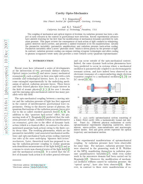
a r X i v :0712.1618v 1 [p h y s i c s .o p t i c s ] 10 D e c 2007Cavity Opto-MechanicsT.J.Kippenberg ∗Max Planck Institut f¨u r Quantenoptik,Garching,Germanyand K.J.Vahala 2†California Institute of Technology,Pasadena,USAThe coupling of mechanical and optical degrees of freedom via radiation pressure has been a sub-ject of early research in the context of gravitational wave detection.Recent experimental advanceshave allowed studying for the ﬁrst time the modiﬁcations of mechanical dynamics provided by radi-ation pressure.This paper reviews the consequences of back-action of light conﬁned in whispering-gallery dielectric micro-cavities,and presents a uniﬁed treatment of its two manifestations:notably the parametric instability (parametric ampliﬁcation)and radiation pressure back-action cooling.Parametric instability oﬀers a novel ”photonic clock”which is driven purely by the pressure of light.In contrast,radiation pressure cooling can surpass existing cryogenic technologies and oﬀers cooling to phonon occupancies below unity and provides a route towards cavity Quantum OptomechanicsI.INTRODUCTIONRecent years have witnessed a series of developments at the intersection of two,previously distinct subjects.Optical (micro-)cavities[1]and micro (nano)mechanical resonators[2],each a subject in their own right with a rich scientiﬁc and technological history,have,in a sense,be-come entangled experimentally by the underlying mech-anism of optical,radiation pressure forces.These forces and their related physics have been of major interest in the ﬁeld of atomic physics[3,4,5,6]for over 5decades and the emerging opto-mechanical context has many par-allels with this ﬁeld.The opto-mechanical coupling between a moving mir-ror and the radiation pressure of light has ﬁrst appeared in the context of interferometric gravitational wave ex-periments.Owing to the discrete nature of photons,the quantum ﬂuctuations of the radiation pressure forces give rise to the so called standard quantum limit [7,8,9].In addition to this “quantum back-action ”eﬀect,the pio-neering work of V.Braginsky[10]predicted that the radi-ation pressure of light,conﬁned within an interferometer (or resonator),gives rise to the eﬀect of dynamic back-action (which is a classical eﬀect,in contrast to the afore-mentioned quantum back-action)owing to the ﬁnite cav-ity decay time.The resulting phenomena,which are the parametric instability (and associated mechanical oscilla-tion)and opto-mechanical back-action cooling represent two sides of the same underlying “dynamic back-action”mechanism .Later,theoretical work has proposed to us-ing the radiation-pressure coupling to realize quantum non-demolition measurements of the light ﬁeld[11]and as a means to create non-classical states of the light ﬁeld[12]and the mechanical system[13].It is noted that the ef-fect of dynamic back-action is of rather general relevance2diation pressure,the dynamic manifestations of radia-tion pressure forces on micro-and nano-mechanical ob-jects have only recently become an experimental real-ity.Curiously,while the theory of dynamic back ac-tion was motivated by consideration of precision mea-surement in the context of gravitational wave detection using large interferometers[19],theﬁrst observation of this mechanism was reported in2005at a vastly diﬀer-ent size scale in microtoroid cavities[20,21,22].These observations were focused on the radiation pressure in-duced parametric instability[19].Subsequently,the re-verse mechanism[23](back-action cooling)has been ex-ploited to cool cantilevers[24,25,26],microtoroids[27] and macroscopic mirror modes[28,29]as well as me-chanical nano-membranes[30].We note that this tech-nique is diﬀerent than the earlier demonstrated radiation-pressure feedback cooling[28,31],which uses electronic feedback analogous to“Stochastic Cooling”[32]of ions in storage rings and which can also provide very eﬃcient cooling as demonstrated in recent experiments[26,33, 34].Indeed,research in this subject has experienced a remarkable acceleration over the past three years as re-searchers in diverseﬁelds such as optical microcavities[1], micro and nano-mechanical resonators[2]and quantum optics pursue a common set of scientiﬁc goals set for-ward by a decade-old theoretical framework.Indeed, there exists a rich theoretical history that considers the implications of optical forces in this new context. Subjects ranging from entanglement[35,36];genera-tion of squeezed states of light[12];to measurements at or beyond the standard quantum limit[11,37,38]; and even to tests of quantum theory itself are in play here[39].On the practical side,there are opportuni-ties to harness these forces for new metrology tools[34] and even for new functions on a semiconductor chip (e.g.,oscillators[20,21],optical mixers[40],and tune-able opticalﬁlters and switches[41,42].It seems clear that a newﬁeld of cavity optomechanics has emerged, and will soon evolve into cavity quantum optomechanics (cavity QOM)whose goal is the observation and explo-ration of quantum phenomena of mechanical systems[43] as well as quantum phenomena involving both photons and mechanical systems.The realization of dynamical, opto-mechanical coupling in which radiation forces me-diate the interaction,is a natural outcome of underly-ing improvements in the technologies of optical(micro) cavities and mechanical micro(nano-)resonators.Re-duction of loss(increasing optical and mechanical Q) and reductions in form factor(modal volume)have en-abled a regime of operation in which optical forces are dominant[20,21,25,27,29,29,30,33,34,42].This coupling also requires coexistence of both high-Q opti-cal and high-Q mechanical modes.Such coexistence has been achieved in the geometries illustrated in Figure1. It also seems likely that other optical microcavity ge-ometries such as photonic crystals[44]can exhibit the dynamic back-action eﬀect provided that structures are modiﬁed to support high-Q mechanical modes.To understand how the coupling of optical and me-chanical degrees of freedom occurs in any of the depicted geometries,one need only consider the schematic in the upper panel of Figure1.Here,a Fabry-Perot optical cavity is assumed to feature a mirror that also functions as a mass-on-a-spring(i.e.is harmonically suspended). Such a conﬁguration can indeed be encountered in grav-itational wave laser interferometers(such as LIGO)and is also,in fact,a direct representation of the“cantilever mirror”embodiment in the lower panel within Figure1. In addition it is functionally equivalent to the case of a microtoroid embodiment(also shown in the lower panel), where the toroid itself provides both the optical modes as well as mechanical breathing modes(see Figure1and discussion below).Returning to the upper panel,inci-dent optical power that is resonant with a cavity mode creates a large circulating power within the cavity.This circulating power exerts a force upon the“mass-spring”mirror,thereby causing it to move.Reciprocally,the mir-ror motion results in a new optical round trip condition, which modiﬁes the detuning of the cavity resonance with respect to the incidentﬁeld.This will cause the system to simply establish a new,static equilibrium condition. The nonlinear nature of the coupling in such a case can manifest itself as a hysteretic behavior and was observed over two decades ago in the work by Walther et.al[17]. However,if the mechanical and optical Q’s are suﬃciently high(as is further detailed in what follows,such that the mechanical oscillation period is comparable or exceeds the cavity photon lifetime)a new set of dynamical phe-nomena can emerge,related to mechanical ampliﬁcation and cooling.In this paper,we will give theﬁrst uniﬁed treatment of this subject.Although microtoroid optical microcavities will be used as an illustrative platform,the treatment and phenomena are universal and pertain to any cavity opto-mechanical systems supporting high Q optical and mechanical modes.In what follows we begin with a the-oretical framework through which dynamic back-action can be understood.The observation of micromechani-cal oscillation will then be considered by reviewing both old and new experimental results that illustrate the ba-sic phenomena[20,21,22].Although this mechanism has been referred to as the parametric instability,we show that it is more properly deﬁned in the context of me-chanical ampliﬁcation and regenerative oscillation.For this reason,we introduce and deﬁne a mechanical gain, its spectrum,and,correspondingly,a threshold for oscil-lation.Mechanical cooling is introduced as the reverse mechanism to ampliﬁcation.We will then review the experimental observation of cooling by dynamic back-action[27,45]and also the quantum limits of cooling us-ing back action[46,47].Finally,we will attempt to discuss some of the possible future directions for this newﬁeld of research.3 II.THEORETICAL FRAMEWORK OFDYNAMIC BACK-ACTIONA.Coupled Mode EquationsDynamic back-action is a modiﬁcation of mechanicaldynamics caused by non-adiabatic response of the opticalﬁeld to changes in the cavity size.It can be understoodthrough the coupled equations of motion for optical andmechanical modes,which can be derived from a singleHamiltonian[48].da2τ0+11dt2+Ωmdt+Ω2m x=F RP(t)m eff=ζT rt+F L(t)2τ=12τexand∆(x)=ω−ω0(x)accounts for the detuning of the pump laser frequency ωwith respect to the cavity resonanceω0(x)(which,as shown below,depends on the mechanical coordinate,x). The power coupling rate into outgoing modes is described by the rate1/τex,whereas the intrinsic cavity loss rate is given by1/τ0.In the subsequent discussion,the photon decay rate is also usedκ≡1/τ.The second equation describes the mechanical coordi-nate(x)accounting for the movable cavity boundary(i.e. mirror),which is assumed to be harmonically bound and undergoing harmonic oscillation at frequencyΩm with a power dissipation rateΓm=Ωmc|a|2T rt ).Moreover the termF L(t)denotes the random Langevin force,and obeys F L(t)F L(t′) =Γm k B T R m effδ(t−t′),where k B is the Boltzmann constant and T R is the temperature of the reservoir.The Langevin force ensures that theﬂuctua-tion dissipation theorem is satisﬁed,such that the total steady state energy in the(classical)mechanical mode E m(in the absence of laser radiation)is given by E m= Ω2m eff|χ(Ω)F L(Ω)|2dΩ=k B T R,where the mechan-ical susceptibilityχ(Ω)=m−1eff/(iΩΓm+Ω2m−Ω2)has been introduced.Of special interest in theﬁrst equation is the optical detuning∆(x)which provides coupling to the second equation through the relation:∆(x)=∆+ω0x) of the above set of equations,it becomes directly evident that the equilibrium position of the mechanical oscillator will depend upon the intra-cavity power.Since the lat-ter is again coupled to the mechanical displacement,this leads to a cubic equation for the mirror positionτex|s|2=cm effx 4τ2 ∆+ω0x 2+1 (4)For suﬃciently high power,this leads to bi-stable be-havior(namely for a given detuning and input power the mechanical position can take on several possible values).B.Modiﬁcations due to Dynamic Back-action:Method of Retardation ExpansionThe circulating optical power will vary in response to changes in the coordinate”x”.The delineation of this response into adiabatic and non-adiabatic contributions provides a starting point to understand the origin of dy-namic back-action and its two manifestations.This de-lineation is possible by formally integrating the above equation for the circulatingﬁeld,and treating the term x wihin it as a perturbation.Furthermore,if the time variation of x is assumed to be slow on the time scale of the optical cavity decay time(or equivalently ifκ≫Ωm) then an expansion into orders of retardation is possible. Keeping only terms up to dx4in mechanical oscillator equation)can be expressed as follows,P cav =P 0cav+P 0cav8∆τ2R x −τP 0cav8∆τ2RdxT rt=τ4∆2τ2+1|s |2denotesthe power in the cavity for zero mechanical displace-ment.The circulating power can also be written as P 0cav =F /π·C ·|s |2,where C =τ/τexT rt denotes the cavity Finesse.The ﬁrst twoterms in this series provide the adiabatic response of the optical power to changes in position of the mir-ror.Intuitively,they give the instantaneous variations in coupled power that result as the cavity is “tuned”by changes in “x ”.It is apparent that the x −dependent contribution to this adiabatic response (when input to the mechanical-oscillator equation-of-motion through the forcing function term)provides an optical-contribution to the stiﬀness of the mass-spring system.This so-called “optical spring”eﬀect (or ”lightinduced rigidity”)has been observed in the context of LIGO[18]and also in microcavities[52].The corresponding change in spring constant leads to a frequency shift,relative to the un-pumped mechanical oscillator eigenfrequency,as given by (where P =|s |2denotes the input power):∆Ωm =κ≫Ωm F 28n 2ω0(4τ2∆2+1)P (6)The non-adiabatic contribution in equation5is propor-tional to the velocity of the mass-spring system.When input to the mechanical-oscillator equation,the coeﬃ-cient of this term is paired with the intrinsic mechanical damping term and leads to the following damping rate given by (for a whispering gallery mode cavity of radius R ):Γ=κ≫Ωm−F 38n 3ω0R(4τ2∆2+1)2P (7)Consequently,the modiﬁed (eﬀective)damping rate of the mechanical oscillator is given by:Γeff =Γ+Γm(8)In both equation 6and 7we have stressed the fact that these expressions are valid only in the weak retar-dation regime in which κ≫Ωm .The sign of Γ(and the corresponding direction of power ﬂow)depends upon the relative detuning of the optical pump with respect to the cavity resonant frequency.In particular,a red-detuned pump (∆<0)results in a sign such that op-tical forces augment intrinsic mechanical damping,whileFIG.2:The two manifestations of dynamic back-action:blue-detuned and red-detuned pump wave (green)with respect tooptical mode line-shape (blue)provide mechanical ampliﬁca-tion and cooling,respectively.Also shown in the lower panels are motional sidebands (Stokes and anti-Stokes ﬁelds)gen-erated by mirror vibration and subsequent Doppler-shifts of the circulating pump ﬁeld.The amplitudes of these motional sidebands are asymmetric owing to cavity enhancement of the Doppler scattering process.a blue-detuned pump (∆>0)reverses the sign so that damping is oﬀset (negative damping or ampliﬁcation).It is important to note that the cooling rate in the weak-retardation regime depends strongly (∝F 3)on the opti-cal ﬁnesse,which has been experimentally veriﬁed as dis-cussed in section 4.2.Note also that maximum cooling or ampliﬁcation rate for given power occurs when the laser is detuned to the maximum slope of the cavity lorenzian;these two cases are illustrated in Figure 1.These mod-iﬁcations have been ﬁrst derived by Braginsky[10]more than 3decades ago and are termed dynamic back-action .Speciﬁcally,an optical probe used to ascertain the po-sition of a mirror within an optical resonator,will have the side-eﬀect of altering the dynamical properties of the mirror (viewed as a mass-spring system).The direction of power-ﬂow is also determined by the sign of the pump frequency detuning relative to cavity resonant frequency.Damping (red tuning of the pump)is accompanied by power ﬂow from the mechanical mode to the optical mode.This ﬂow results in cooling of the mechanical mode.Ampliﬁcation (blue tuning of pump)is,not surprisingly,accompanied by net power ﬂow from the optical mode to the mechanical mode.This case has also been referred to as heating ,however,it is more ap-propriately referred to as ampliﬁcation since the power ﬂow in this direction performs work on the mechanical mode.The nature of power ﬂow between the mechani-cal and optical components of the system will be explored here in several ways,however,one form of analysis makes contact with the thermodynamic analogy of cycles in a Clapeyron or Watt diagram (i.e.a pressure-volume di-5FIG.3:Work done during one cycle of mechanical oscilla-tion can be understood using a PV diagram for the radiationpressure applied to a piston-mirror versus the mode volumedisplaced during the cycle.In this diagram the cycle followsa contour that circumscribes an area in PV space and hencework is performed during the cycle.The sense in which thecontour is traversed(clockwise or counterclockwise)dependsupon whether the pump is blue or red detuned with respectto the optical mode.Positive work(ampliﬁcation)or negativework(cooling)are performed by the photon gas on the pistonmirror in the corresponding cases.agram).In the present case–assuming the mechanicaloscillation period to be comparable to or longer than thecavity lifetime–such a diagram can be constructed to an-alyze powerﬂow resulting from cycles of the coherent ra-diation gas interacting with a movable piston-mirror[53](see Figure3).In particular,a plot of radiation pressureexerted on the piston-mirror versus changes in opticalmode volume provides a coordinate space in which it ispossible to understand the origin and sign of work doneduring one oscillation cycle of the piston mirror.Consid-ering the oscillatory motion of the piston-mirror at someeigenfrequencyΩm,then because pressure(proportionalto circulating optical power)and displaced volume(pro-portional to x)have a quadrature relationship(throughthe dynamic back-action term involving the velocity dx6 in accordance with the abovemodel.FIG.4:Dynamics in the weak retardation regime.Experi-mental displacement spectral density functions for a mechani-cal mode with eigenfrequency40.6MHz measured using three, distinct pump powers for both blue and red pump detuning. The mode is thermally excited(green data)and its linewidth can be seen to narrow under blue pump detuning(red data) on account of the presence of mechanical gain(not suﬃcient in the present measurement to excite full,regenerative oscil-lations);and to broaden under red pump detuning on account of radiation pressure damping(blue data).Figure4presents such lineshape data taken using a microtoroid resonator.The power spectral density of the photocurrent is measured for a mechanical mode at an eigenfrequency of40.6MHz;three spectra are shown,corresponding to room temperature intrinsic mo-tion(i.e.negligible pumping),mechanical ampliﬁcation and cooling.In addition to measurements of ampliﬁ-cation and damping as a function of pump power(for ﬁxed detuning),the dependence of these quantities on pump detuning(with pump powerﬁxed)can also be measured[27].Furthermore,pulling of the mechanical eigenfrequency(caused by the radiation pressure modi-ﬁcation to mechanical stiﬀness)can also be studied[52].A summary of such data measured using a microtoroid in the regime whereκ Ωm is provided in Figure5. Both the case of red-(cooling)and blue-(ampliﬁcation) pump detuning are shown.Furthermore,it can be seen that pump power was suﬃcient to drive the mechani-cal system into regenerative oscillation over a portion of the blue detuning region(section of plot where linewidth is nearly zero).For comparison,the theoretical predic-tion is shown as the solid curve in the plots.Concerning radiation-pressure-induced stiﬀness,it should be noted that for red-detuning,the frequency is pulled to lower frequencies(stiﬀness is reduced)while for blue-detuning the stiﬀness increases and the mechanical eigenfrequency shifts to higher values.This is in dramatic contrast to similar changes that will be discussed in the next section. While in Figure5the absolute shift in the mechanical eigenfrequency is small compared toΩm,it is interesting to note that it is possible for this shift to be large.Specif-ically,statically unstable behavior is possible if the total spring constant reaches a negative value.This has in-deed been observed experimentally in gram scale mirrors coupled to strong intra-cavityﬁelds by the LIGO groupat MIT[29].FIG.5:Upper panel shows mechanical linewidth(δm=Γef f/2π)and shift in mechanical frequency(lower panel) measured versus pump wave detuning in the regime where Ωm≪κ.For negative(positive)detuning cooling(ampliﬁca-tion)occurs.The region between the dashed lines denotes the onset of the parametric oscillation,where gain compensates mechanical loss.Figure stems from reference[27].Solid curves are theoretical predictions based on the sideband model(see section2.2).While the above approach provides a convenient wayto understand the origin of gain and damping and their relationship to non-adiabatic response,a more generalunderstanding of the dynamical behavior requires an ex-tension of the formalism.Cases where the mechanicalfrequency,itself,varies rapidly on the time scale of the cavity lifetime cannot be described correctly using theabove model.From the viewpoint of the sideband pic-ture mentioned above,the modiﬁed formalism must in-clude the regime in which the sideband spectral separa-tion from the pump can be comparable or larger than the cavity linewidth.C.Sideband FormalismIt is important to realize that the derivation of thelast section only applies to the case where the condi-tionκ≫Ωm is satisﬁed.In contrast,a perturbativeexpansion of the coupled mode equations(eqns.1and 2)gives an improved description that is also valid in theregime where the mechanical frequency is comparable to or even exceeds the cavity decay rate(whereΩm≫κis the so called resolved sideband regime).The derivation that leads to these results[27]is outlined here.For mostexperimental considerations(in particular for the case of7 cooling)the quantityε=x1i∆−12i(∆+Ωm)τ−1+e−iΩm tc|a|2c|a|2 cT rtω0τ2/τex4(∆+Ωm)2τ2+1−2(∆−Ωm) cT rtω0τ2/τex4(∆+Ωm)2τ2+1−2τcT rtω01/τex2R×2τ4(∆−Ωm)2τ2+1 P(12)This quantity can be recognized as the diﬀerence inintra-cavity energy of anti-Stokes and Stokes modes,i.e.P m =(|a AS|2−|a S|2)/T rt,as expected from energyconservation considerations.Consequently,this analysisreveals how the mechanical mode extracts(ampliﬁcation)or loses energy(cooling)to the opticalﬁeld,despite thevastly diﬀerent frequencies.Cooling or ampliﬁcation ofthe mechanical mode thus arises from the fact that thetwo side-bands created by the harmonic mirror motionare not equal in magnitude,due to the detuned nature ofthe excitation(see Figure2).In the case of cooling,a reddetuned laser beam will cause the system to create moreanti-Stokes than Stokes photons entailing a net powerﬂow from the mechanical mode to the opticalﬁeld.Con-versely,a blue-detuned pump will reverse the sidebandasymmetry and cause a net powerﬂow from the opticalﬁeld to the mechanical mode,leading to ampliﬁcation.We note that in the case of cooling,the mechanism issimilar to the cooling of atoms or molecules inside an op-tical resonator via”coherent scattering”as theoreticallyproposed[54]and experimentally observed[55].From thepower calculation,the cooling or mechanical ampliﬁca-tion rateΓ= P mΩm m eff c2C×14(∆+Ωm)2τ2+1 P(13)Here theﬁnesse F has been introduced(as before)aswell as the previously introduced dimensionless couplingfactor C=τ/τex2Ωm 14(∆+Ωm)2τ2+1=8∆2τ8 Hence as noted before,in the weak retardation regime,the maximum cooling(or ampliﬁcation)rate for a givenpower occurs when the laser is detuned to the maximumslope of the cavity lorenzian;i.e.|∆|=κ/2,in closeanalogy to Doppler cooling[6]in Atomic Physics.Onthe other hand,in the resolved sideband regime opti-mum detuning occurs when the laser is tuned either tothe lower or upper“motional”sideband of the cavity,i.e.∆=±Ωm.This behavior is also shown in Figure6.Theabove rate modiﬁes the dynamics of the mechanical oscil-lator.In the case of ampliﬁcation(blue detuned pump)itoﬀsets the intrinsic loss of the oscillator and overall me-chanical damping is reduced.Ultimately,a“thresholdcondition”in which mechanical loss is completely oﬀsetby gain occurs at a particular pump power.Beyond thispower level,regenerative mechanical oscillation occurs.This will be studied in section4below.For red detuning,the oscillator experiences enhanceddamping.Beyond the powerﬂow analysis providedabove,a simple classical analysis can also be used tounderstand how such damping can result in cooling.Speciﬁcally,in the absence of the laser,the mean en-ergy(following from the equation for x)obeys ddt E m =−(Γm+Γ) E m +k B T RΓm(15)Note that within this classical model,the cooling intro-duced by the laser is what has been described by someauthors[28]as“cold damping”:the laser introduces adamping without introducing a modiﬁed Langevin force(in contrast to the case of intrinsic damping).This is akey feature and allows the enhanced damping to reducethe mechanical oscillator temperature,yielding as aﬁ-nal eﬀective temperature for the mechanical mode underconsideration:T eff∼=ΓmΓm+Γ>1Ωm m eff c2Cτ×∆−Ωm4(∆+Ωm)2τ2+1 P(17)Note that in the regime where the mechanical fre-quency is comparable to,or exceeds the cavity decayrate it’s behavior is quite diﬀerent from that describedearlier for the conventional adiabatic case;and was onlyrecently observed experimentally[27].As noted earlier,in the adiabatic regime,the mechanical frequency is al-ways downshifted by a red-detuned laser(i.e.a reducedrigidity).However,whenΩm>1/2·κan interestingphenomena can occur.Speciﬁcally,when the pump laserdetuning is relatively small,the mechanical frequencyshift is opposite in sign to the conventional,adiabaticspring eﬀect.The same behavior can occur in the caseof ampliﬁcation(∆>0).Furthermore,a pump de-tuning exists where the radiation-pressure induced me-chanical frequency shift is zero,even while the damp-ing/ampliﬁcation rate is non-zero.The latter has an im-portant meaning as it implies that the entire radiationpressure force is viscous for red detuning,contributingonly to cooling(or to ampliﬁcation for blue detuning).Figure6shows the attained cooling rate(as a contourplot)forﬁxed power and mechanical oscillator frequencyas a function of normalized optical cavity decay rate andthe normalized laser detuning(normalized with respectto∆opt=9An important feature of cooling and ampliﬁcation pro-vided by dynamic back-action is the high level of me-chanical spectral selectivity that is possible.Since,the cooling/ampliﬁcation rates depend upon asymmetry in the motional sidebands,the optical line-width and pump laser detuning can be used to select a particular mechan-ical mode to receive the maximum cooling or ampliﬁca-tion.In eﬀect,the damping/ampliﬁcation rates shown above have a spectral shape (and spectral maximum)that can be controlled in anexperimental setting as given by horizontal cuts of Figure 6.This feature is important since it can provide a method to control oscillation fre-quency in cases of regenerative oscillation on the blue detuning of the pump.Moreover,it restricts the cooling power to only one or a relatively small number of me-chanical modes.In cases of cooling,this means that the overall mechanical structure can remain at room temper-ature while a target mechanical mode is refrigerated.FIG.7:Dynamics in the regime where Ωm ∼κas reported in Ref.[27].Upper panel shows the induced damping /am-pliﬁcation rate (δm =Γef f /2π)as a function of normalized detuning of the laser at constant power.The points repre-sent actual experiments on toroidal microcavities,and the solid line denotes a ﬁt using the sideband theoretical model (Equations 13and 17).Lower panel shows the mechanical frequency shift as a function of normalized detuning.Arrow denotes the point where the radiation pressure force is entirely viscous causing negligible in phase,but a maximum quadra-ture component.The region between the dotted lines denotes the onset of the parametric instability (as discussed in section 3).Graph stems from Ref.[27].The full-eﬀect of the radiation-pressure force (both the in-phase component,giving rise to a mechanical fre-quency shift,and the quadrature-phase component which can give rise to mechanical ampliﬁcation/cooling)were studied in a “detuning series”,as introduced in the last section.The predictions made in the Ωm >0.5κregime have been veriﬁed experimentally as shown in Figure 7.Speciﬁcally,the predicted change in the rigidity of theoscillator was experimentally observed as shown in Fig-ure 7and is in excellent agreement with the theoretical model (solid red line).Keeping the same sample but us-ing a diﬀerent optical resonance with a line-width of 113MHz (57.8MHz mechanical resonance),the transition to a pure increasing and decreasing mechanical frequency shift in the cooling and ampliﬁcation regimes was ob-served as shown in the preceding section,again conﬁrm-ing the validity of our theoretical model based on the motional sidebands.III.OPTOMECHANICAL COUPLING AND DISPLACEMENT MEASUREMENTS A.Mechanical Modes of Optical MicrocavitiesThe coupling of mechanical and optical modes in a Fabry Perot cavity with a suspended mirror (as ap-plying to the case of gravitational wave detectors)or mirror on a spring (as in the case of a cantilever)is easily seen to result from momentum transfer upon mirror reﬂection and can be described by a Hamilto-nian formalism[48].It is,however,important to real-ize that radiation pressure coupling can also occur in other resonant geometries:notably in the class of optical-whispering-gallery-mode (WGM)microcavities such as microspheres[56],microdisks[57]and microtoroids[58](see Figure 8).Whereas in a Fabry Perot cavity the mo-mentum transfer occurs along the propagation direction of the conﬁned photons[10],the mechanism of radiation pressure coupling in a whispering gallery mode cavity occurs normal to the optical trajector[20,21,22].This can be understood to result from momentum conserva-tion of the combined resonator-photon system as pho-tons,trapped within the whispering gallery by continu-ous total-internal reﬂection,execute circular orbits.In particular,their orbital motion necessitates a radial ra-diation pressure exerted onto the cavity boundary.The latter can provide coupling to the resonator’s mechanical modes.While the mechanical modes of dielectric microspheres are well known and described by analytic solutions (the Lamb theory),numerical ﬁnite-element simulations are required to calculate the frequency,as well as strain and stress ﬁelds,of more complicated structures (exhibiting lower symmetry)such as micro-disks and micro-toroids.In the case of a sphere[59],two classes of modes ex-ist.Torsional vibrations exhibit only shear stress with-out volume change,and therefore no radial displacement takes place in these modes.Consequently these modes cannot be excited using radiation pressure,which re-lies upon a change in the optical path length (more for-mally,these modes do not satisfy the selection rule of opto-mechanical coupling,which requires that the inte-gral of radiation pressure force and strain does not van-ish along the optical trajectory).In contrast,the class of modes for which volume change is present is referred to。

电子类文献中英文翻译(发电机)

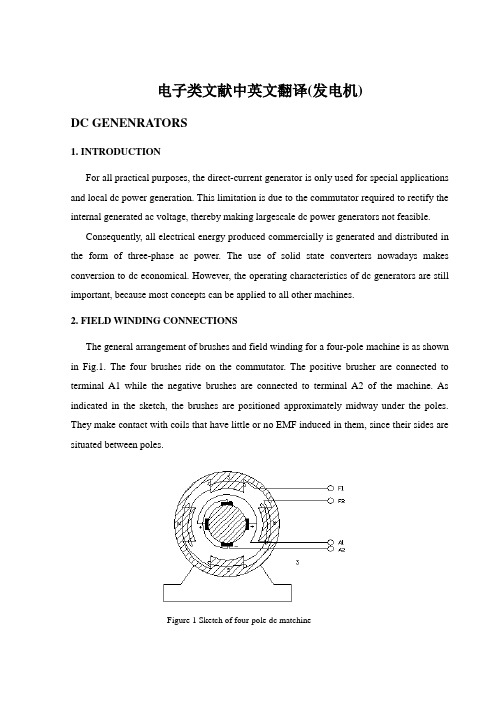
电子类文献中英文翻译(发电机)DC GENENRATORS1. INTRODUCTIONFor all practical purposes, the direct-current generator is only used for special applications and local dc power generation. This limitation is due to the commutator required to rectify the internal generated ac voltage, thereby making largescale dc power generators not feasible.Consequently, all electrical energy produced commercially is generated and distributed in the form of three-phase ac power. The use of solid state converters nowadays makes conversion to dc economical. However, the operating characteristics of dc generators are still important, because most concepts can be applied to all other machines.2. FIELD WINDING CONNECTIONSThe general arrangement of brushes and field winding for a four-pole machine is as shown in Fig.1. The four brushes ride on the commutator. The positive brusher are connected to terminal A1 while the negative brushes are connected to terminal A2 of the machine. As indicated in the sketch, the brushes are positioned approximately midway under the poles. They make contact with coils that have little or no EMF induced in them, since their sides are situated between poles.Figure 1 Sketch of four-pole dc matchineThe four excitation or field poles are usually joined in series and their ends brought out to terminals marked F1 and F2. They are connected such that they produce north and south poles alternately.The type of dc generator is characterized by the manner in which the field excitation is provided. In general, the method employed to connect the field and armature windings falls into the following groups (see Fig.2):Figure2 Field connections for dc generators:(a)separately excited generator;(b)self-excited,shunt generator;(c)series generator;(d)compound generator;short-shunt connection;(e)compoundgenerator,long-shunt connection.The shunt field contains many turns of relatively fine wire and carries a comparatively small current, only a few percent of rated current. The series field winding, on the other hand, has few turns of heavy wire since it is in series with the armature and therefore carries the load current.Before discussing the dc generator terminal characteristics, let us examine the relationship between the generated voltage and excitation current of a generator on no load. The generated EMF is proportional to both the flux per pole and the speed at which the generator is driven, EG=kn. By holding the speed constant it can be shown the EG depends directly on the flux.To test this dependency on actual generators is not very practical, as it involves a magnetic flux measurement. The flux is produced by the ampere-turns of the field coils: in turn, the flux must depend on the amount of field current flowing since the number of turns on the field winding is constant. This relationship is not linear because of magnetic saturation after the field current reaches a certain value. The variation of EG versus the field current If may be shown by a curve known as the magnetization curve or open-circuit characteristic. For this a given generator is driven at a constant speed, is not delivering load current, and has its field winding separately excited.The value of EG appearing at the machine terminals is measured as If is progressively increased from zero to a value well above rated voltage of that machine. The resulting curve is shown is Fig.3. When Ij=0, that is, with the field circuit open circuited, a small voltage Et is measured, due to residual magnetism. As the field current increases, the generated EMF increases linearly up to the knee of the magnetization curve. Beyond this point, increasing the field current still further causes saturation of the magnetic structure to set in.Figure 3 Magnetization curve or open-circuit characteristic of a separately excited dc machineThe means that a larger increase in field current is required to produce a given increase in voltage.Since the generated voltage EG is also directly proportional to the speed, a magnetization curve can be drawn for any other speed once the curve is determined. This merely requires anadjustment of all points on the curve according ton n x E E G G ''=where the quantities values at the various speeds.3. VOLTAGE REGULATIONLet us next consider adding a load on generator. The terminal voltage will then decrease (because the armature winding ha resistance) unless some provision is made to keep it constant. A curve that shows the value of terminal voltage for various load currents is called the load or characteristic of the generator.Figure 4 (a) directs current it to urge the generator load characteristics; (b) circuit diagramFig.4 shows the external characteristic of a separately excited generator. The decrease in the terminal voltage is due mainly to the armature circuit resistance RA. In general,A A G t R I E V -=where Vt is the terminal voltage and IA is the armature current (or load current IL) supplied by the generator to the load.Another factor that contributes to the decrease in terminal voltage is the decrease in flux due to armature reaction. The armature current established an MMF that distorts the main flux, resulting in a weakened flux, especially in noninterpole machines. This effect is calledarmature reaction. As Fig.4 shows, the terminal voltage versus load current curve does not drop off linearly since the iron behaves nonlinear. Because armature reaction depends on the armature current it gives the curve its drooping characteristic.4. SHUNT OR SELF-EXCIITED GENRATORSA shunt generator has its shunt field winding connected in parallel with the armature so that the machine provides its own excitation, as indicated in Fig.5. The question arises whether the machine will generate a voltage and what determines the voltage.For voltage to “build up” as it is called, there must be some remanent magnetism in the field poles. Ordinarily, if the generator has been used previously, there will be some remanent magnetism. We have seen in Section 3 that if the field would be disconnected, there will be small voltage Ef generated due to this remanent magnetism, provided that the generator is driven at some speed. Connecting the field for self-excitation, this small voltage will be applied to the shunts field and drive a small current through the field circuit. If this resulting small current in the shunt field is of such a direction that it weakens the residual flux, the voltage remains near zero and the terminal voltage does not build up. In this situation the weak main pole flux opposes the residual flux.Figure 5 Shunt generator:(a)circuit;(b)load characteristicIf the connection is such that the weak main pole flux aids the residual flux, the inducedvoltage increases rapidly to a large, constant value. The build-up process is readily seen to be cumulanve. That is, more voltage increases the field current, which in turn increases the voltage, and so on. The fact that this process terminates at a finite voltage is due to the nonlinear behavior of the magnctic circuit. In steady state the generated voltage is causes a field current to flow that is just sufficient to develop a flux required for the generated EMF that causes the field current to flow.The circuit carries only dc current, so that the field current depends only on the field circuit resistance, Rf. This may consist of the field circuit resistance Rf, the field current depends on the generated voltage in accordance with Ohm ’s law.It should be evident that on a new machine or one that has lost its residual flux because of a long idle period, some magnetism must be created. This is usually done by connecting the field winding only to a separate dc source for a few seconds. This procedure is generally known as flashing the field.Series GeneratorsAs mentioned previously, the field winding of a series generator is in series with the armature. Since it carries the load current the series field winding consists of only a few turns of thick wire. At no load, the generated voltage is small due to residual field flux only. When a load is added, the flux increases, and so does the generated voltage. Fig.7 shows the load characteristic of a series generator driven at a certain speed. The dashed line indicates the generated EMF of the same machine with the armature open-circuited and the field separately excited. The difference between the two curves is simply the IR drop in the series field and armature winding, such that)(S A A G t R R I E V +-=where RS is the series field winding resistance.Figure 7 Series generator: (a)circuit diagram;(b)load characteristicsCompound GeneratorsThe compound generator has both a shunt and a series field winding, the latter winding wound on top of the shunt winding. Fig.8 shows the circuit diagram. The two windings are usually connected such that their ampere-turns act in the same direction. As such the generator is said to be cumulatively compounded.The shunt connection illustrated in Fig.8 is called a long shunt connection. If the shunt field winding is directly connected across the armature terminals, the connection is referred to as a short shunt. In practice the connection used is of little consequence, since the shunt field winding carries a small current compared to the full-load current. Furthermore, the number of turns on the series field winding. This implies it has a low resistance value and the corresponding voltage drop across it at full load is minimal.Curves in Fig.9 represents the terminal characteristic of the shunt field winding alone. By the addition of a small series field winding the drop in terminal voltage with increased loading is reduced as indicated. Such a generator is said to be undercompounded. By increasing the number of series turns, the no-load and full-load terminal voltage can be made equal; the generator is then said to be flatcompounded. If the number of series turns is more than necessary to compensate for the voltage drop, the generator is overcome pounded. In that case the full-load voltage is higher than the no-load voltage.Figure 9 Terminal characteristics of compound generators compared with that of the shunt generatorThe overcompounded generator may be used in instances where the load is at some distance from the generator. The voltage drops in the feeder lines are the compensated for with increased loading. Reversing the polarity of the series field in relation to the shunt field, the fields will oppose each other more and more as the load current increase. Such a generator is said to be differentially compounded. It is used in applications where feeder lines could occur approaching those of a short circuit. An example would be where feeder lines could break and short circuit the generator. The short-circuit current, however, is then limited to a “safe” value. The terminal characteristic for this type of generator is also shown in Fig.9. Compound generators are used more extensively than the other types because they may be designed to have a wide varity of terminal characteristics.As illustrated, the full-load terminal voltage can be maintained at the no-load value by the proper degree of compounding. Other methods of voltage control are the use of rheostats, for instance, in the field circuit. However, with changing loads it requires a constant adjustment of the field rheostat to maintain the voltage. A more useful arrangement, which is now common practice, is to use an automatic voltage regulator with the generator. In essence, the voltage regulator is a feedback control system. The generator output voltage is sensed and compared to a fixed reference voltage deviation from the reference voltage gives an error signal that is fed to a power amplifier. The power amplifier supplies the field excitation current. If the error signal is positive, for example, the output voltage is larger than desiredand the amplifier will reduce its current drive. In doing so the error signal will be reduced to zero.TRANSFORMER1. INTRODUCTIONThe high-voltage transmission was need for the case electrical power is to be provided at considerable distance from a generating station. At some point this high voltage must be reduced, because ultimately is must supply a load. The transformer makes it possible for various parts of a power system to operate at different voltage levels. In this paper we discuss power transformer principles and applications.2. TOW-WINDING TRANSFORMERSA transformer in its simplest form consists of two stationary coils coupled by a mutual magnetic flux. The coils are said to be mutually coupled because they link a common flux. In power applications, laminated steel core transformers (to which this paper is restricted) are used. Transformers are efficient because the rotational losses normally associated with rotating machine are absent, so relatively little power is lost when transforming power from one voltage level to another. Typical efficiencies are in the range 92 to 99%, the higher values applying to the larger power transformers.The current flowing in the coil connected to the ac source is called the primary winding or simply the primary. It sets up the flux φ in the core, which varies periodically both in magnitude and direction. The flux links the second coil, called the secondary winding or simply secondary. The flux is changing; therefore, it induces a voltage in the secondary by electromagnetic induction in accordance with Lenz’s law. Thus the primary receives its power from the source while the secondary supplies this power to the load. This action is known as transformer action.3. TRANSFORMER PRINCIPLESWhen a sinusoidal voltage V p is applied to the primary with the secondary open-circuited, there will be no energy transfer. The impressed voltage causes a small current Iθ to flow in the primary winding. This no-load current has two functions: (1) it produces the magnetic flux in the core, which varies sinusoidally between zero and φm, where φm is the maximum value of the core flux; and (2) it provides a component to account for the hysteresis and eddy current losses in the core. There combined losses are normally referred to as the core losses.The no-load current Iθ is usually few percent of the rated full-load current of the transformer (about 2 to 5%). Since at no-load the primary winding acts as a large reactance due to the iron core, the no-load current will lag the primary voltage by nearly 90º. It is readily seen that the current component I m= I0sinθ0, called the magnetizing current, is 90ºin phase behind the primary voltage V P. It is this component that sets up the flux in the core; φ is therefore in phase with I m.The second component, I e=I0sinθ0, is in phase with the primary voltage. It is the current component that supplies the core losses. The phasor sum of these two components represents the no-load current, orI0 = I m+ I eIt should be noted that the no-load current is distortes and nonsinusoidal. This is the result of the nonlinear behavior of the core material.If it is assumed that there are no other losses in the transformer, the induced voltage In the primary, E p and that in the secondary, E s can be shown. Since the magnetic flux set up by the primary winding，there will be an induced EMF E in the secondary winding in accordance with Faraday’s law, namely, E=NΔφ/Δt. This same flux also links the primary itself, inducing in it an EMF, E p. As discussed earlier, the induced voltage must lag the flux by 90º, therefore, they are 180º out of phase with the applied voltage. Since no current flows in the secondary winding, E s=V s. The no-load primary current I0 is small, a few percent of full-load current. Thus the voltage in the primary is small and V p is nearly equal to E p. The primary voltage and the resulting flux are sinusoidal; thus the induced quantities E p and E s vary as a sine function. The average value of the induced voltage given byE avg = turns× change in flux in a given time given timewhich is Faraday’s law applied to a finite time interval. It follows thatE avg = N 21/(2)m f = 4fNφm which N is the number of turns on the winding. Form ac circuit theory, the effective or root-mean-square (rms) voltage for a sine wave is 1.11 times the average voltage; thusE = 4.44fNφmSince the same flux links with the primary and secondary windings, the voltage per turn in each winding is the same. HenceE p = 4.44fN p φmandE s = 4.44fN s φmwhere E p and Es are the number of turn on the primary and secondary windings, respectively. The ratio of primary to secondary induced voltage is called the transformation ratio. Denoting this ratio by a, it is seen that a = p sE E = p s N N Assume that the output power of a transformer equals its input power, not a bad sumption in practice considering the high efficiencies. What we really are saying is that we are dealing with an ideal transformer; that is, it has no losses. ThusP m = P outorV p I p × primary PF = V s I s × secondary PFwhere PF is the power factor. For the above-stated assumption it means that the power factor on primary and secondary sides are equal; thereforeV p I p = V s I s from which is obtainedp s V V = p s I I ≌ p sE E ≌ aIt shows that as an approximation the terminal voltage ratio equals the turns ratio. The primary and secondary current, on the other hand, are inversely related to the turns ratio. The turns ratio gives a measure of how much the secondary voltage is raised or lowered in relation to the primary voltage. To calculate the voltage regulation, we need more information.The ratio of the terminal voltage varies somewhat depending on the load and its power factor. In practice, the transformation ratio is obtained from the nameplate data, which list the primary and secondary voltage under full-load condition.When the secondary voltage V s is reduced compared to the primary voltage, the transformation is said to be a step-down transformer: conversely, if this voltage is raised, it is called a step-up transformer. In a step-down transformer the transformation ratio a is greater than unity (a>1.0), while for a step-up transformer it is smaller than unity (a<1.0). In the event that a=1, the transformer secondary voltage equals the primary voltage. This is a special type of transformer used in instances where electrical isolation is required between the primary and secondary circuit while maintaining the same voltage level. Therefore, this transformer is generally knows as an isolation transformer.As is apparent, it is the magnetic flux in the core that forms the connecting link between primary and secondary circuit. In section 4 it is shown how the primary winding current adjusts itself to the secondary load current when the transformer supplies a load.Looking into the transformer terminals from the source, an impedance is seen which by definition equals V p / I p . From p s V V = p s I I ≌ p sE E ≌ a , we have V p = aV s and I p = I s /a.In terms of V s and I s the ratio of V p to I p isp p V I = /s s aV I a= 2s s a V I But V s / I s is the load impedance Z L thus we can say thatZ m (primary) = a 2Z LThis equation tells us that when an impedance is connected to the secondary side, it appears from the source as an impedance having a magnitude that is a 2 times its actual value. We say that the load impedance is reflected or referred to the primary. It is this property oftransformers that is used in impedance-matching applications.4. TRANSFORMERS UNDER LOADThe primary and secondary voltages shown have similar polarities, as indicated by the “dot-making” convention. The dots near the upper ends of the windings have the same meaning as in circuit theory; the marked terminals have the same polarity. Thus when a load is connected to the secondary, the instantaneous load current is in the direction shown. In other words, the polarity markings signify that when positive current enters both windings at the marked terminals, the MMFs of the two windings add.Since the secondary voltage depends on the core flux φ0, it must be clear that the flux should not change appreciably if E s is to remain essentially constant under normal loading conditions. With the load connected, a current I s will flow in the secondary circuit, because the induced EMF E s will act as a voltage source. The secondary current produces an MMF N s I s that creates a flux. This flux has such a direction that at any instant in time it opposes the main flux that created it in the first place. Of course, this is Lenz’s law in action. Thus the MMF represented by N s I s tends to reduce the core flux φ0. This means that the flux linking the primary winding reduces and consequently the primary induced voltage E p, This reduction in induced voltage causes a greater difference between the impressed voltage and the counter induced EMF, thereby allowing more current to flow in the primary. The fact that primary current I p increases means that the two conditions stated earlier are fulfilled: (1) the power input increases to match the power output, and (2) the primary MMF increases to offset the tendency of the secondary MMF to reduce the flux.In general, it will be found that the transformer reacts almost instantaneously to keep the resultant core flux essentially constant. Moreover, the core flux φ0drops very slightly between n o load and full load (about 1 to 3%), a necessary condition if E p is to fall sufficiently to allow an increase in I p.On the primary side, I p’ is the current that flows in the primary to balance the demagnetizing effect of I s. Its MMF N p I p’ se ts up a flux linking the primary only. Since the core flux φ0 remains constant. I0 must be the same current that energizes the transformer at no load. Theprimary current I p is therefore the sum of the current I p’ and I0.Because the no-load current is relatively small, it is correct to assume that the primary ampere-turns equal the secondary ampere-turns, since it is under this condition that the core flux is essentially constant. Thus we will assume that I0 is negligible, as it is only a small component of the full-load current.When a current flows in the secondary winding, the resulting MMF (N s I s) creates a separate flux, apart from the flux φ0 produced by I0, which links the secondary winding only. This flux does no link with the primary winding and is therefore not a mutual flux.In addition, the load current that flows through the primary winding creates a flux that links with the primary winding only; it is called the primary leakage flux. The secondary- leakage flux gives rise to an induced voltage that is not counter balanced by an equivalent induced voltage in the primary. Similarly, the voltage induced in the primary is not counterbalanced in the secondary winding. Consequently, these two induced voltages behave like voltage drops, generally called leakage reactance voltage drops. Furthermore, each winding has some resistance, which produces a resistive voltage drop. When taken into account, these additional voltage drops would complete the equivalent circuit diagram of a practical transformer. Note that the magnetizing branch is shown in this circuit, which for our purposes will be disregarded. This follows our earlier assumption that the no-load current is assumed negligible in our calculations. This is further justified in that it is rarely necessary to predict transformer performance to such accuracies. Since the voltage drops are all directly proportional to the load current, it means that at no-load conditions there will be no voltage drops in either winding.中文翻译①直流发电机1.介绍关于所有实际目的来说，直流发电机仅用于特殊场合与地方性发电厂。

大修后文章直接录用

5. Response to comment: Point is entitled "stability and repeatability of ******s". Somequestions: Here, it is shown the dependence of SERS relative intensities of SC on time. Is it the same sample (******-adsorbate) that is stored and then SERS spectra are recorded at different times or instead, the same ****** is stored and then the adsorbate is added at different times and thereafter the SERS spectra are recorded Authors should clarify the procedure. Are different results expected with these two procedures Have been these two methods checked It is possible that only ******s stored without adsorbate are active for a longer timeExperimentally it is often observed that roughed surface in SERS produces molecular degradation and a comparation between Raman and SERS spectra is necessary to identify the molecular fundamental modes. Why the authors did not record Raman spectra of SC Raman spectra should be added to Fig. 5. The point should be because a characteristic of surface is explained and must follow point . The old becomes . Moreover, old epigrap****** 3.2.1. and should be removed and a unique point . should be presented instead and entitled " Biocompatibility of ******s. SERS spectra of ****** and ******". Also, epigraph must be removed and the text must follow to the new section .Response: We are very sorry for our unclear report in the section of .For the first question proposed by the Reviewer, our answer is as following:Yes, in the section of , the main intention is to display the stability and reproducibility of Agnanofilms. Fig. 6 (in the original manuscript, Fig. 5 in the revised manuscript) shows the dependence of SERS relative intensities of SC on time. In this section, the ******s are stored and then the adsorbate is added at different times and thereafter the SERS spectra are recorded. For the second question proposed by Reviewer, our answer is as following:As the Reviewer's good instruction, we have clarified the procedure in the revised manuscript.However, in this study, we have not studied the first procedure of the same sample (******-adsorbate) that is stored and then SERS spectra are recorded at different times. Thus, these two methods have not been checked. Take the time limit of the submission of the revised manuscript into account; it is difficult to carry out the first procedure in the revised manuscript. However, we appreciate for the Reviewers’ good advice earnestly. We will check these two procedures in future studies. For the third question proposed by Reviewer, our answer is as following: According to the Reviewer's good instruction, we have recorded Raman spectra of SC in solid state, as shown in Fig. 1(a) (Fig. 4(a) in revised manuscript). Meanwhile, the points and have also been re-written according to the instructions proposed by the Reviewer. (See the section of and 3.3 in the revised manuscript)图略spectrum of (a) solid SC. SERS spectra of ×10mol/L SC aqueous solutionadsorbed on (b) glass slide, (c) ******-Ag CNPs, and (d) ******, respectively.6. Response to comment: Sentence "the number of spectra for every condition is five" (page 9) or the number of spectra is 5 (Table 1 and 2), what does it mean Perhaps something like this: EachSERS spectrum is recorded 5 times in different points of the ****** surface？Response: As the Reviewer's good question, the sentence of “the number of spectra for everycondition is five" or “the number of spectra is 5 (Table 1 and 2)” in the original manuscr ipt is hard to be understood.This sentence means that each SERS spectrum is recorded 5 times in differpoints of the ****** surface. we have revised this sentence in the revised manuscript according to the Reviewer's advice.7. Response to comment: Epigrap****** of Table 1 and 2 should be revised. Corrections are indicatedin the manuscript.Response: According to the Reviewer's good instruction, we have revised the epigrap****** of Table1 and 2. The epigraph of Table 1 “Table 1 Preliminary assignations of the Raman bands (Mean ± ., n=5) for the SERS spectra of ******. The number of spectra is 5” is revised as“Assignments for the SERS bands (Mean ± ., n=5) of ****** (based on Refs. [25-30]).”The epigraph of Table 2 “Table 2 Observed wavenumbers (Mean ± ., n=5), assignments,and local coordinates of ******, excited at 785 nm. The number of spectra is 5. [35-37]” is revised as “Table 2Assignments for the SERS bands (Mean ± ., n=5) of ****** (based on Refs. [32-34]).”8. Response to comment: Figure 4 shows SERS spectra of ****** and ****** recorded on different Ag nanofilms. What do authors want to say This experiment is to check the reproducibility of the method Thus, it is better to use the word "reproducibility" and not "repeatability". This must be clarified in the text.Response: As the Reviewer's good advice, we should use the word “reproducibility” and not"repeatability". Figure 4 (in the original manuscript) shows SERS spectra of ****** and ****** recorded on the different ******s prepared under the same conditions. The authors want to display the reproducibility of the ******s prepared by this simple method. Thus, we have replaced theword "repeatability" by "reproducibility" in the revised manuscript.9. Response to comment: Uv-vis absorption spectrum of不******-protected Ag nanoparticules shows a maximum at 418 nm and at 785 nm the absorbance is zero (Figure 1b). Given that SERS spectra are recorded at 785 nm, I think that this excitation line is very far from the maximum to obtain a good signal. In fact, the Raman signal is very weak (Figure 3). Is it possible to obtain a better signal employing another excitation laser, for example, 514nm I mean, probably the 785nm line is better for ****** than for ******-protected Ag nanoparticules, but under other different excitation laser the ******-protected Ag nanoparticules could be a good substrate for ****** or ******. Have been checked different excitation laser linesResponse: We are very sorry for our negligence of the explanation for why SERS spectra of ******and ****** are recorded at 785 nm. In the studying of the SERS effect of ****** and ******, we think that the excitation with the 785 nm wavelength has a number of advantageous features compared to [a] other wavelengt******. A previous study has reported that a laser wavelength shorter than nm is known to enhance photodissociation and cause protein degradation even at a low power. However, the sample damage can be avoided using laser light of a longer wavelength. No paling effects were observed using laser light with wavelength ≥660 nm. In their study, degradation of the biological objects was observed when using nm excitation lasers. Meanwhile, it is known that when using 660 nm irradiation, for a laser power of 10mW and a diameter of 10 μm, 2the light intensity is up to 127 MW/m . In our system, the laser power is set at 65mW and the 2 3 2 diameter is 90μm. So the light intensity was ca. 10 MW/m(10 W/cm ), which is much smaller than that of 660 nm irradiation. Thus, in our studies, we employed a 65-mW, 785-nm diode laser to record the Raman and SERS spectra of ****** and ****** in order to avoid the photodissociation and degradation of the proteins.[a] G. J. Puppels, J. H. F. Olminkhof, G. M. J. Segers-Nolten, C. Otto, F. F. M. Demul, J. Greve. Laser Irradiation and Raman Spectroscopy of Single Living Cells and Chromosomes: Sample Degradation Occurs with nm but not with 660 nm Laser Light . Exp. Cell Res, 195 (1991) 361.Special thanks to you for your good comments.Reviewer 4#1. Response to comment: I'm not familiar with blood sample preparation but I wasn't able to extract the final concentration of ****** and ****** added to the ******-NPs and ******. This value has to be clearly reported in the text. Response: As the Reviewer suggested that we have calculated the final concentration of ****** and ****** added to the ******-protected ****** (******-Ag CNPs) and ****** in the revised manuscript. According our calculation, the final concentration of ****** and ****** added to ****** is ca.4.8 and %, respectively. However, take the dilution of the Ag colloid into account, the final concentration of ****** and ****** added to the ******-Ag CNPs is and %, respectively. All these concentrations have been added in the revised the final concentrations of ****** added to the ******-NPs and ****** are different, the quantity of ****** lighted by the laser spot based on ****** g) equals to (in order of magnitude) that based on ******-Ag CNP samples (ca. ×10g). Similarly, the quantity of ****** lighted by the laser spot based on ****** g) equals to (in order of magnitude) that based on ******-Ag CNPs (ca. ×10g). Take the SERS detection of ****** for example: For the SERS detection of ****** based on ******-Ag CNPs, the probe volume is considered a focal [b]“tube”with a waist diameter of 90 m and a depth of ca. 1cm. By using the concentration of ****** %) one can determine the quantity of ****** molecules contributing to the Raman intensity ( (1000+60) ×10×% × (45 ×10 )×1×10 / [(1000+60)×10 ] ~ ×10g). For the SERS detection of ****** based on ******, supposing that all the ****** molecules adsorbed on the surface of ****** evenly, one can determine the quantity of ****** molecules contributing to the Raman intensity (~ (50) ×10×% × (45 ×10 )/ (5 ×10 )~ ×10g).[b] L. Baia, K. Gigant, U. Posset, et al. Appl. Spectrosc, 56 (2002) 536.(2) Response to comment: In the experimental results section does not appear how the SERSmeasurements on ******-NPs were performed.Response: We are very sorry for our negligence of introduce how the SERS measurements on ******-Ag CNPs were performed in the experimental results section. As Reviewer suggested that we have made complementarities of this experimental process in the section of of the revised manuscript. (the section of , 16-20 lines)(3) Response to comment: A significant comparison between the SERS activities of ******-NPsand ****** substrates is not possible based on what reported in the paper. For instance, is thenumber of NPs lighted by the laser spot equals for ******-NP and ****** samples The authors have to make clear to the reader what they are comparing. Moreover, the normal Raman of ****** and ****** in solution and/or in solid state in fig. 3 would be helpful to understand the effect of the metal-analyte interaction.Response: We are very sorry for our unclear description of what the SERS activities of ******-NPsand ****** substrates are comparing. In Fig 3 of the original manuscript (Fig 8 in revisedmanuscript ), we mainly want to tell the reader the ******-Ag CNPs are unfit for the SERS detectionof ****** and ******, compared to the ******s prepared by electrostatic self-assembly with the******-Ag CNPs. That is, the SERS effect of ******-Ag CNPs for ****** and ****** is much weaker than that of ******. According to the Reviewer good question (“is the number of NPs lighted by the laser spot equals for ******-NP and ****** samples”), we have calculated the number of NPs lighted by the laser spot for ******-Ag CNPs and ******s. The calculation results show that the number of NPs lighted by the laser spot is not equal for ******-Ag CNPs and ******s. One can calculate the concentration of the ******-Ag CNPs in Ag colloid is ca. ×10 /m according to the electrochemical reaction in our work. For the SERS detection based on ******-Ag CNPs, the probe volume was considered a focal “tube” with a waist diameter of 90 m and a depth of ca. 1cm. By using the concentration of ******-Ag CNPs in Ag colloid ×10 /m ) one can determine the number of NPs lighted by the laser spot ×10 × (45×10 )×1×10 ~ ×10 ). For the SERS detection based on ******, by supposing that thedistribution of the NPs on the surface of ****** is uniform, one can determine the number of NPs lighted by the laser spot ( (45 ×10 )/ (200 ×10 /2)~×10). It can be seen that, the number of NPs lighted by the laser spot for ******-Ag CNPs is more than that for ******s. However, the experimental results show that the SERS effect of ****** and ****** on ******-Ag CNPs is much weaker than that on ******s, indicating that the SERS activity of ******s is better than that of ******-Ag CNPs. As the Reviewer suggested that, we have recorded the normal Raman scattering of ****** and ****** in solid state, as shown in Fig 2A(c) and Fig 2B(c), respectively. Very weak Raman signals are observed from solid ****** and ******. We know that Raman spectroscopy is a powerful tool that gives precise information on the vibration energies of molecules, and can provide the fingerprint for unique chemical identification. However, the Raman scattering cross section of most biologicalmacromolecules is extremely small, which causes the Raman signals of biological[c]macromolecules are very difficult to obtain . Thus, in this paper, we attempt to obtain new SERS substrates to solve this question. Such as the Ag nanofilms prepared by using e lectrostatic self-assembly with the ******-Ag CNPs in this work.图略Fig. 2. (a) Raman spectrum of (A) solid ****** and (B) solid ******. SERS spectra of (A) ****** and (B)****** solution adorbed on (b) ******-Ag CNPs and (c) ******, respectively.[c] ,, Appl. Phys. Lett. 91 (2005) 223105.(4) Response to comment: It is quite expected that larger EM enhancement occurson aggregated NPs adsorbed on the glass slide with respect to the un-aggregated ******-NPs. As far as I understood, the key point of the paper is the fabrication of ****** with interparticle regions of ca. 300 nm where the ****** and ****** molecules can be located, leading then to intense SERS signals. Therefore, this new substrate should be compared to other silver nanofilms which do not present these cavities, in order, also, to give some evidences to the previous hypothesis, which is a mere speculation based on the results reported in the article.Response: As the Reviewer suggested that we have checked the new substrate with another silvernanofilm which dose not present these cavities. Fig.3a (following) shows the SEM image of acommon ****** prepared using coupling agent of cysteamine and common Ag NPs on thesurface of the glass slide. It shows that the average size of the particles on the surface of this common ****** is ca.75 ± 5 nm, which is much smaller than that (200 ± 50 nm) of theparticles on the surface of the new ****** prepared using electrostatic self-assembly with******-Ag CNPs . Meanwhile, single layer of Ag nanoparticles is observed and no lots ofnano-scale regions are formed on the surface of the common ******. (following) shows the SERS spectra of ****** solution %, 50 L) on this common Ag nanofilm (Fig.4 a) and the new ****** with a diameter of 1 cm, respectively. It shows that the EM enhancement occurs on the common ****** is weaker than that on the new ******. Meanwhile, striking spectral differences are seen in SERS spectra at 812, and 1022 cm , indicating that the orientation of the adsorbed ****** molecules is different on these two ******s. We think that it is mainly related to the surface characteristics of this new Ag nanofilm. On the surface of the new ******, the average size of the aggregated particles is up to ca. 200 ± 50 nm, which is much larger than that of the common ******. It improves the adsorption ability of the ****** molecules onto the surface of the new ****** effectively. Meanwhile, lots of nano-scale regions with the size of ca. 300 ± 50 nm are formed between the adjacent nanoparticles on the surface of the new ******, which makes ****** molecules can be embedded in effectively. It implies that the presence of nano-scale regions on the surface of the new ****** is an important factor for SERS effect of biologicalmacromolecules.图略. SEM image of the ****** prepared by using coupling agent of cysteamine (a) and byusing electrostatic self-assembly with ******-Ag CNPs (b) on glass slide.图略Fig. 4. SERS spectra of ****** solution %) on (a) the common ****** prepared by usingcoupling agent of cysteamine and common Ag nanoparticles and (b) on the ****** prepared byusing electrostatic self-assembly with ******-Ag CNPs, respectively.(5) Response to comment: The SERS spectra showed in fig. 5c is doubtfully assigned to ******. I suggest to the authors to carry out control experiments so that to rule out the presence of impurities on their silver film. In the following paper is reported the SERS spectrum of Citrate anion on silver NPs: Title: Anomalous Raman bands appearing in surface-enhanced Raman spectra Author(s): Sanchez-Cortes, S; Garcia-Ramos, JV Source: JOURNAL OF RAMAN SPECTROSCOPY Volume: 29 Issue: 5 Pages: 365-371 Published: MAY 1998Response: We are very grateful for your providing of the reference above. We have read this reference carefully. As Sanchez-Cortes et al. reported that the ions and new molecular speciesresulting from the reduction of the metal will remain in the colloid system (especially in the citrate colloids), which has an obvious impact on the SERS of the analyte. Thus, in our present work, we employed the method of electrolysis to obtain ******-Ag CNPs, and employed the method of electrostatic self-assembly to obtain ******s. In our experiment of preparation of ******-Ag CNPs, ****** was not employed act as reducing agent in order to avoid the effect of citrate anion on the SERS of the analyte recorded on the surface of the new ****** the Reviewer’s good instruction, we have carried out a control experiment. In this control experiment, we have checked the Raman scattering on the surfaceof the new ********s prepared under the same conditions, as shown in following Fig .5. The experimental results show that the effect of the impurities on the surfaces of these ******s on the SERS of the analyte is negligible. Meanwhile, as reported by Sanchez-Cortes et al., the Raman spectrum of solid citrate is shown [d]in Fig. 6 a. We can see that the main SERS bands of solid citrate recorded by us (Fig. 7) are close to the Raman bands of solid citrate reported by Sanchez-Cortes et al.图略. Raman spectra of the surfaces of the different ******s (a, b, c, d) prepared usingelectrostatic self-assembly with ******-Ag CNPs.图略Fig. 6. Effect of excitation wavelength on the SERS background of an aggregated citrate colloid:(A) FT-Raman spectrum of solid citrate (λex=l 064 nm); (B) FT-Raman spectrum of aqueous citrate (2 M, λex=l 064 nm); (C) FT-SER spectrum of the aggregated colloid after addition of NO3(0.05 M) (λex=1064nm); (D) SERS spectrum of the same sam ple with excitation at nm.图略Fig. 7. SERS spectra of ****** based on ****** prepared by using electrostaticself-assembly with ******-Ag CNPs.[d] S. S. Corte and J. V. G. Ramos. Anomalous Raman Bands Appearing in Surface-EnhancedRaman Spectra. JOURNAL OF RAMAN SPECTROSCOPY. 29 (1998) 365.Special thanks to you for your good comments and suggestions！Dear Editors and Reviewers.We have tried our best to revise and improve the manuscript and made great changes in themanuscript according to the Reviwers′good comments. And here we did not list the changes butmarked in red in revised paper.We appreciate for Editors/Reviewers’ warm work earnestly, and hope that the corrections willmeet with approval.Once again, thank you very much for your comments and suggestions.We look forward to your information about my revised papers and thank you for your goodcomments.Yours sincerely,. Liu。

Elektrotechnik含词汇注释

Elektronische SchaltungInhaltsverzeichnis目录[Verbergen]∙ 1 Aufgabengebieteo 1.1 Energietechnik能源技术o 1.2 Antriebstechnik电力拖动技术、电气传动技术o 1.3 Nachrichtentechnik通信技术o 1.4 Elektronik电子技术o 1.5 Automatisierungstechnik自动化技术o 1.6 Elektronische Gerätetechnik电气设备o 1.7 Theoretische Elektrotechnik理论电工∙ 2 Geschichte历史, Entwicklungen发展und Personen人物der Elektrotechnik o 2.1 Anfänge im 17. und 18. Jahrhunderto 2.2 19. Jahrhunderto 2.3 20. Jahrhundert∙ 3 Elektrotechnik in der Berufswelt职业领域o 3.1 Studienfach专业o 3.2 Ausbildungsberufe职业培训o 3.3 Berufsverbände职业手册∙ 4 Siehe auch∙ 5 Literatur参考文献∙∙Die klassische Einteilung典型的分类der Elektrotechnik war die Starkstromtechnik强电技术, die heute in der Energietechnik能源技术 und der Antriebstechnik电力拖动技术 ihrenNiederschlag findet, und die Schwachstromtechnik弱电技术, die sich zur Nachrichtentechnik通信技术formierte. Als weitere Gebiete kamen die elektrische Messtechnik检测技术unddie Regelungstechnik自动控制原理sowie die Elektronik 电子技术hinzu. Die Grenzen 边界zwischen den einzelnen Bereichen sind dabei vielfach多重的fließend. Mit zunehmender 日益增加的Verbreitung扩展der Anwendungen应用ergaben sich zahllose无数的weitereSpezialisierungsgebiete特殊领域. In unserer heutigen Zivilisation公共事业werden fast alle Abläufe und Einrichtungen设备elektrisch betrieben运行oder laufen运行unter wesentlicher Beteiligung elektrischer Geräte und Steuerungen控制.Energietechnik能源技术[Bearbeiten]ÜbertragungsleitungDie elektrische Energietechnik (früher Starkstromtechnik强电技术) befasst包含sich mit der Gewinnung获得、生产, Übertragung传输und Umformung变换elektrischer Energie und auch der Hochspannungstechnik高压技术. Elektrische Energie wird in den meisten Fällen在绝大多数情况下durch Wandlung变换aus mechanisch机械的-rotatorischer旋转的Energiemittels Generatoren发电机，发生器erzeugt产生. Zur klassischen Starkstromtechnik gehören außerdem der Bereich der Verbraucher负载elektrischer Energie sowie die Antriebstechnik电力拖动. Zu dem Bereich der Übertragung elektrischer Energie im Bereich der Niederspannung低电压zählt auch der Themenbereich der Elektroinstallationen电气装备, wie sie unter anderemvielfältig im Haushalt家务zu finden sind.Anfänge im 17. und 18. Jahrhundert [Bearbeiten]Luigi Galvani伽伐尼Science理学学士zu erwerben申请, dann beträgt die Regelstudienzeit 6 Semester, an der FH 7 Semester inklusive Praxissemester.Das Studium der Elektrotechnik beinhaltet 包含einige themenverwandte Fächer与主题相关的课程: Grundlagen der Elektrotechnik电工原理, Physik物理,Höhere Mathematik,高等数学Netzwerk- und Systemtheorie网络与系统理论, Regelungstechnik, 自动控制原理Nachrichtentechnik通讯技术, elektromagnetische Verträglichkeit电磁兼容 (EMV), einige Laborpraktika实验und Spezialisierungsfächer特殊的课程. An der Universität wird die wissenschaftliche Arbeit科研工作in der Ausbildung进修、学习betont强调, an der Fachhochschule steht die Anwendung应用physikalischer Kenntnisse im Vordergrund突出. Aufgrund der Interdisziplinarität跨学科und der oft engen Verflechtung mit der Informatik信息学, ist auch Programmieren编程in der Regel Teil des Studiums. Entsprechende相应的Studiengänge专业oder eng 相近的，密切的verwandte Studiengänge heißen dann auch etwa Elektro- und Informationstechnik电气信息技术bzw. technische Informatik工程信息学.Der …Doktor-Ingenieur“博士工程师、工学博士ist der höchste akademische Grad学位, derüblicherweise通常地im Anschluss an ein einschlägiges 有关的、相关的Studium an einer Universität erreicht取得、实现werden kann.An einigen Hochschulen kann das Fach Elektro- und Informationstechnik信息技术auch in sieben Semestern mit der Aussicht 前景、前途auf den Master硕士für Berufliche Bildung studiert werden, der weitere drei Semester umfasst包含. Mit diesem Abschluss und weiteren 1,5 Jahren Referandariatszeit 实习期、见习期kann man einer Stell Komponenten e als Gewerbelehrer 职业教师(höherer Dienst) an einer Berufsschule职业学校 nachgehen. Ebenso existiert das Studienfach Lehramt an Berufsschulen für Elektrotechnik; hier wird üblicherweise ebenfalls ein Referendariat实习生gefordert, bevor eine Stelle im höheren Dienst更高的职位an einer Berufsschule angetreten竞争werden kann.Ausbildungsberufe职业教育[Bearbeiten]→Hauptartikel: Liste der Ausbildungsberufe in der ElektrotechnikBerufsverbände [Bearbeiten]Der größte Berufsverband für Elektrotechnik weltweit ist das Institute of Electrical & Electronics Engineers(IEEE). Er zählt über 400.000 Mitglieder成员und publiziert出版Zeitschriften 杂志auf allen relevanten Fachgebieten相关的学科领域in Englisch. Seit 2008 gibt es den IEEE Global History Network (IEEE GHN), wobei in verschiedenen Kategorien分类、关键词wichtige Meilensteine里程碑(beurteilt durch ein Fachgremium专家小组、事务委员会) und persönliche Erinnerungen回忆、回忆录、纪要von Ingenieuren (IEEE First-Hand) festgehalten werdenkönnen. Ein solcher Erinnerungsbericht回忆录、报告eines Schweizer Elektroingenieurs kann als Beispiel eingesehen看作为werden.[1]Portal:Elektrotechnik– Übersicht zu Wikipedia-Inhalten zum Thema ElektrotechnikPortal:Mikroelektronik– Übersicht zu Wikipedia-Inhalten zum Thema Mikroelektronik▪Manfred Albach: Grundlagen der Elektrotechnik 1. Erfahrungssätze, Bauelemente, Gleichstromschaltungen.Pearson Studium, München 2004, ISBN 3-8273-7106-6.▪Manfred Albach: Grundlagen der Elektrotechnik 2. Periodische und nicht periodische Signalformen. Pearson Studium, München 2005, ISBN 3-8273-7108-2.▪Gert Hagmann: Grundlagen der Elektrotechnik. 11., durchges. Aufl., Wiebelsheim 2005, ISBN 3-89104-687-1.▪Winfield Hill, Paul Horowitz: Die hohe Schule der Elektronik, Tl.1, Analogtechnik.Elektor-Verlag 2002 ISBN 3-89576-024-2.▪Winfield Hill, Paul Horowitz: Die hohe Schule der Elektronik, Tl.2, Digitaltechnik.Elektor-Verlag 1996 ISBN 3-89576-025-0.▪Helmut Lindner, Harry Brauer, Constanz Lehmann: Taschenbuch der Elektrotechnik und Elektronik. 9. neu bearbeitete Auflage. Fachbuchverlag Leipzig im Carl-Hanser-Verlag 2008, ISBN 978-3-446-41458-7.Weblinks [Bearbeiten]Wiktionary: Elektrotechnik– Bedeutungserklärungen, Wortherkunft, Synonyme,ÜbersetzungenWikibooks: Formelsammlung Elektrotechnik– Lern- und LehrmaterialienWikibooks: Formelsammlung Elektrizitätslehre– Lern- und LehrmaterialienWikibooks: Regal:Elektrotechnik– Lern- und Lehrmaterialien。

电子科学与技术专业外语翻译

Figure 1-1】图1－1 给出了在三种材料中一些重要材料相关的电阻值（相应电导率ρ≡1/δ)。

However】然而锗不太适合在很多方面应用因为温度适当提高后锗器件会产生高的漏电流。

For a given】对于给定的半导体，存在代表整个晶格的晶胞，通过在晶体中重复晶胞组成晶格。

This structure】这种结构也属于金刚石结构并且视为两个互相贯穿的fcc亚点阵结构，这个结构具有一个可以从其它沿立方对角线距离的四分之一处移动的子晶格（位移/4）Most of】多数Ⅲ-Ⅴ半导体化合物具有闪锌矿结构，它与金刚石有相同结构除了一个有Ⅲ族Ga原子的fcc子晶格结构和有Ⅴ族As原子的另一个。

.For example】例如，孤立氢原子的能级可由玻尔模型得出：式中m0 代表自由电子质量, q是电荷量,ε0是真空中电导率, h 是普朗克常数，n 是正整数称为主量子数。

Further decrease】空间更多减少将导致能带从不连续能级失去其特性并合并起来，产生一个简单的带。

As shown】如图1－4（a）能带图所示，有一个大带隙。

注意到所有的价带都被电子充满而导带中能级是空的As a consequence】结果，半满带的最上层电子以及价带顶部电子在获得动能（外加电场）时可以运动到与其相应的较高能级上At room】在室温和标准大气压下，带隙值硅（1.12ev ）砷化镓（1.42ev）在0 K带隙研究值硅（1.17ev ）砷化镓（1.52ev）Thus】于是，导带的电子密度等于把N(E)F(E)dE从导带底Ec （为简化起见设为0）积分到导带顶EtopFigure 1-5】图1-5从左到右示意地表示了本征半导体的能带图, 态密度(N(E)~E1/2), 费米分布函数, 本征半导体的载流子浓度In an extrinsi c】在非本征半导体中，一种载流子类型增加将会通过复合减少其它类型的数目；因此，两种类型载流子的数量在一定温度下保持常数For shallow】对硅和砷化镓中的浅施主,在室温下,常常有足够的热能电离所有的施主杂质,给导带提供等量的电子We shal l】我们先讨论剩余载流子注入的概念。

多通道碳阴极活化过一硫酸盐降解水中有机物的性能

大连理工大学硕士学位论文摘要活化的过硫酸盐氧化，作为一种新兴的高级氧化技术，是一种矿化难降解有毒污染物的有效方法。

在众多的活化方法中，过硫酸盐通过接受电子完成的电化学活化，具有容易操控和环境友好的特点，被认为是一种有前景的活化技术。

但在电化学活化的过程中，由于静电斥力阻碍了过硫酸盐阴离子和阴极之间的接触，导致过硫酸盐低的分解率和随后低的自由基的产生量，从而使污染物的降解效果变差。

针对此问题，本文使用天然木材衍生的碳化木（CW）制备了具有多通道的流通式阴极（FTC），通过将过一硫酸盐（PMS）阴离子限制在阴极的微通道中，能够显著地强化其与阴极的碰撞与接触，提高电化学活化的效率并增强对污染物的降解。

主要的研究成果如下：（1）通过天然松木的一步碳化制备并组装了具有丰富的介孔，良好的导电性，较高的机械强度，大量有序的微通道以及对PMS有良好的电催化活性的FTC。

以苯酚为目标污染物，探究了不同的反应条件（PMS浓度、电流密度和停留时间）对FTC电活化PMS降解苯酚性能的影响。

结果表明，在苯酚进水浓度为20 mg/L, 进水TOC=18 mg/L，进水PMS浓度为6.51 mM，背景Na2SO4为0.05 M，电流密度为2.75 mA/cm2，进水pH 2.87，停留时间10 min以及常温的条件下，通过FTC电活化PMS，PMS的分解率达到了71.9%。

苯酚和TOC的去除率分别达到了97.9%和39.6%。

EPR实验结果表明，在FTC电活化PMS的过程中，产生了大量的·OH和SO4•-。

同时，自由基淬灭实验也表明，·OH和SO4•-均参与了对苯酚的降解，且·OH对降解的贡献更大。

此外，五次循环实验的结果证明了本研究组装的FTC具有很好的稳定性。

（2）通过封闭CW的微通道，获得了流过式阴极（FBC）。

在相同的优化条件下，详细对比了在FTC中和FBC上的PMS的分解、自由基的产量以及电活化PMS降解三种酚类有机物（苯酚、双酚A和4-氯苯酚）的性能。

kink效应

100IEEE ELECTRON DEVICE LETTERS,VOL.30,NO.2,FEBRUARY2009 Anomalous Kink Effect in GaN HighElectron Mobility TransistorsGaudenzio Meneghesso,Senior Member,IEEE,Franco Zanon,Michael J.Uren,Member,IEEE,and Enrico Zanoni,Fellow,IEEEAbstract—An anomalous kink effect has been observed in the room-temperature drain current I D versus drain voltage V DS characteristics of GaN high electron mobility transistors.The kink is originated by a buildup(at low V DS)and subsequent release (at high V DS)of negative charge,resulting in a shift of pinch-off voltage V P toward more negative voltages and in a sudden in-crease in I D.The kink is characterized by extremely long neg-ative charge buildup times and by a nonmonotonic behavior as a function of photon energy under illumination.The presence of traps in the GaN buffer may explain both spectrally resolved photostimulation data and the slow negative charge buildup.Index Terms—AlGaN/GaN,GaN,high electron mobility tran-sistor(HEMT),kink effect.I.I NTRODUCTIONK INK effects have been observed in various kinds of FETs, like Si MOSFETs,GaAs MESFETs,and GaAs-and InP-based high electron mobility transistors(HEMTs).Depending on the device structure and layout,on the gate length and on the properties of epitaxial materials,the kink effect may occur at different drain voltage values V DSkink and may have a different bias dependence[1],light sensitivity[2],relationship with im-pact ionization[1],[3],dynamic behavior[3],and dependence on aging and surface treatments[4],[5].Three explanations suggested for the kink effect have been clearly summarized in [2].These are the following:1)channel impact ionization and subsequent hole accumulation leading to changes of surface or channel/substrate interface potential(as in silicon-on-insulator MOSFETs[1]);2)ﬁeld-dependent trapping/detrapping in deep levels;and3)a combined effect of impact ionization and deep levels whereby generated holes modify the occupation state of surface,bulk,or channel/substrate interface deep levels [3].Kink is a detrimental phenomenon for the performance of FETs,possibly resulting in output-conductance increase, transconductance compression,and dispersion between dc and RF characteristics.Recently,kink effects have been described in GaN HEMTs[6]–[10]and were attributed to impact ioniza-tion coupled either withﬂoating-body effects[6],[7]or withManuscript received October9,2008;revised November7,2008.First published December22,2008;current version published January28,2009. This work was supported in part by EDA under the KORRIGAN Project and in part by the Italian Ministry for University and Research under the PRIN2007 Project“GaN wideband microwave and millimeter-wave integrated circuits for low-noise and high-power subsystems,”coordinated by Prof.Giovanni Ghione. The review of this letter was arranged by Editor J.A.del Alamo.G.Meneghesso, F.Zanon,and E.Zanoni are with the Department of Information Engineering,University of Padova,35131Padova,Italy (e-mail:gauss@dei.unipd.it).M.J.Uren is with QinetiQ Ltd.,WR143PS Malvern,U.K.Digital Object Identiﬁer10.1109/LED.2008.2010067traps[9],[10].In this letter,we describe an anomalous kink effect in GaN HEMTs,with a remarkable light sensitivity which is ascribed to the presence of slow traps in the epitaxial layers under the gate,possibly in the GaN buffer.II.S AMPLES AND E XPERIMENTAL R ESULTS AlGaN/GaN HEMTs were grown on4H vanadium-dopedsilicon carbide by MOVPE.The undoped multilayer structureconsisted of a1.2-μm GaN buffer layer,followed by a30-nmAl0.28Ga0.72N barrier layer.The source and drain ohmic con-tacts and gate Schottky contacts were Ti/Al/Pt/Au and Ni/Au,respectively.The devices were passivated using SiN depositedby PECVD.The device gate length and width were0.6and100μm,respectively,the gate-to-drain spacing was2.4μm,andthe drain-to-source distance was4μm.The dc electrical characterization of the devices was carriedout by means of an Agilent HP4142semiconductor parame-ter analyzer;a kink in the dc I D–V DS characteristics wasobserved only when long time constants and slow voltagesweeps were adopted,see Fig.1.For increasing V GS fromthe pinch-off voltage value of≈−6.5–0V,the kink voltageV DSkink(identiﬁed as the point where the output conductanceis maximum)has a nonmonotonic behavior as a function ofV GS.It initially decreases from≈9V(at V GS=−6V)toless than5V(at V GS=−5V)and then increases again up toV DSkink≈10V for V GS=0V.By comparing the I D versus V GS characteristics taken at V DS<V DSkink(hereafter identi-ﬁed as“prekink”region)with those taken at V DS>V DSkink(“postkink”),a shift in the pinch-off voltage V P is evident(see Fig.2).The two threshold voltage values are V p-prekink=−6V and V p-postkink=−6.3V,respectively,the most nega-tive pinch-off voltage value corresponding to the higher drain current measured when V DS>V DSkink.For these devices,the presence of the kink is inﬂuenced only by the properties of the epitaxial layers and was found not to depend on the device fabrication processing(lithography,metallization,annealing processes,plasma treatments,and passivation).In particular, both unpassivated and SiN-passivated devices show the kink. Memory effects can hinder kink characterization during re-peated measurements with a fast sweep rate(provided that V DS exceeds V DSkink during the sweep).Only theﬁrst curve will show a“kink,”i.e.,the kink is temporarily removed as a result of theﬁrst measurement(see the inset of Fig.1).The effect is recovered by keeping the device at V GS=V DS=0V at RT for at least5min.Pulsed measurements(not shown)demonstrate this“memory”effect:If V DS is pulsed from V DS>V DSkink0741-3106/$25.00©2009IEEEMENEGHESSO et al.:ANOMALOUS KINK EFFECT IN GaN HIGH ELECTRON MOBILITY TRANSISTORS101Fig. 1.Long integration time I D versus V DS with a small V GS step (−0.2V from 0to −7V).Gray diamonds correspond to the maximum of the output conductance in the kink region (V KINK ).(Inset)Repeated short integration time I DS versus V DS measurements at V GS =0V.Fig.2.Long integration time I D versus V GS characteristics measured (solid)in the dark and (dashed)under illumination using an incandescent lamp.to V DS <V DSkink ,a very slow decreasing transient of I D is observed (from milliseconds to several seconds depending on the chosen ﬁnal prekink V DS value).When V DS is pulsed from the prekink to the postkink value,I D can reach its high steady-state postkink value in 100μs to 1ms,depending on the ﬁnal bias point.Conventional wisdom suggests that traps may be associated with the charge buildup and transient phenomena related to the kink.In order to investigate a possible role of traps,we carried out dc measurements under continuous illumination and compared them with those obtained in the dark.Rather surprisingly,if the device is illuminated using an incandescent lamp,the kink amplitude increases due to an enhanced prekink shift of pinch-off voltage toward positive values,see Fig.2.We have repeated the characterization using monochromatic light in the 0.8–3.32-eV energy range and measured the amplitude of the kink.Illumination affects the behavior of drain current in the prekink region (see Fig.3).For 1eV <E <2eV,where E is the photon energy,the prekink I D value is lowered,for E >2eV,the prekink I D recovers,and for E >2.5eV,the prekink drain current value is higher than that in the dark.III.D ISCUSSION AND C ONCLUSIONThe long time constants associated with the kink effect suggest the involvement of deep levels,a hypothesis which is conﬁrmed by the peculiar spectral dependence of the kink—the kink amplitude can be modulated using photons withenergiesFig.3.I D values measured at V GS =−3V in postkink region (V DSkink +2V )and in prekink region (V DSkink −2V ))as a function of photon energy from 0.80to 3.32eV .An I D –V DS curve (V GS =−3V )is also presented in the inset to clarify the measurement conditions.Intensity of light sources was kept constant.lower than the GaN energy gap.Deep levels must be located within the epitaxial layers below the gate,since the kink is caused by a shift in V P .This cannot be explained by surface traps;the fact that the kink is not affected by passivation or surface treatments is in agreement with this interpretation.When deep levels are negatively charged,V P is shifted toward more positive values,thus decreasing the drain current:This occurs for V DS <V DSkink or,more slowly,when the device is unbiased.When V DS >V DSkink ,electron detrapping or com-pensation by holes occurs,thus V P returns to more negative values,see Fig.2.The actual mechanism responsible for the modulation of charge on deep levels cannot be due to ﬁeld-assisted detrapping,which should depend monotonically on the electric ﬁeld and,as a consequence,on V GD .Detrapping would be most efﬁcient close to pinch-off,where the V GD and electric ﬁeld are at their maximum.In fact,V DSkink has a nonmonotonic dependence on V GS ,see Fig.1,which is typical of impact-ionization effects [11].When the device is in the ON -state,energetic channel elec-trons could possibly impact ionize traps [11],thus releasing electrons,or can create electron-hole pairs.However,if hole creation by impact ionization does take place,it should be a very rare event,considering the large energy gap of the GaN channel and the low V DS values (≈5–10V)at which the kink occurs,see Fig.1.Moreover,in the electrical conditions corresponding to the occurrence of the kink,we did not observe any of the signs of electron-hole pair creation,like increase in gate current,or photon emission with energy corresponding to the GaN energy gap.A possible mechanism could be the following:When deep levels are negatively charged,electron detrapping can occur due to the impact ionization of traps by hot electrons [12].This requires substantially lower energies than electron-hole pair creation by band-to-band ionization and,consequently,can take place at substantially lower drain voltages.The onset of the kink appears at roughly a constant voltage above the knee volt-age indicating that the hot-electron-assisted detrapping process102IEEE ELECTRON DEVICE LETTERS,VOL.30,NO.2,FEBRUARY2009requires a threshold electricﬁeld and,hence,electron energy.The simultaneous requirement to have a supply of electronsresults in the increase in kink voltage near pinch-off.Illumination with photons with energy E lower than≈1eVdoes not affect the kink.When the device is biased in theprekink region,electron trapping is enhanced by illuminatingthe device with photons having energies between≈1and ≈2eV.A possible explanation could involve the presence of deep states with energies at≈E V+1eV.In this case,photo-stimulation may promote the transfer of an electron from thevalence band to the deep level,resulting in a negatively chargedtrap and reducing|V P|and I D,see Fig.3.When the photon energy exceeds≈2eV,a transition from the deep level to shallow donor states close to E C becomes possible,thus turning on a competitive mechanism removing the negative charge.As a consequence,|V P|and I D recover,and the kink amplitude is reduced,see Fig.3.Similar transitions between deep levels with energies in the2.0–2.5-eV range have been invoked in order to explain the yellow luminescence in GaN[12].Therefore, although traps could be located either within the Al0.28Ga0.72N barrier layer under the gate or in the GaN buffer,spectral data would suggest that they are located in the GaN epitaxial layer. Another consideration which tends to suggest that the traps are located in the GaN is that hot electrons must be present for the detrapping mechanism to occur.In the GaN under the gate(and including the depletion region below the channel), the density of electrons is roughly proportional to V GS−V P, whereas in the AlGaN,the density changes exponentially with gate bias as a result of the rapidly changing electricﬁeld in this region.Hence,the electron density changes much quicker in the AlGaN region,and we would not expect to see the observed V DSkink−V knee behavior.Assuming the presence of deep levels in the GaN buffer re-mote from the2-D electron gas(2DEG),three regimes need tobe considered for prekink trapping dynamics at V DS<V DSkink.1)In unbiased conditions without illumination,only a low con-centration of thermally activated electrons can reach the traps,resulting in an extremely slow trapping and charge buildup rate(hundreds of seconds).2)When the device is unilluminatedand biased in the prekink region,hot electrons from the2DEGcan be injected into the GaN where they can be capturedby traps(the electron concentration is higher than in process1)so that trapping is faster and can take place during typicalvoltage ramp measurements which use a“long”time constantof approximately a second).3)When the device biased in theprekink state is illuminated with monochromatic light withphoton energy E,trapping is promoted for1eV<E<2eV,while detrapping prevails for E>2eV.Although the quotedmechanisms could potentially be applied to trapping/detrappingin the AlGaN,spectroscopic data correspond to those reportedfor deep levels connected to yellow luminescence in GaN[12].In all cases,at V DS>V DSkink,hot electrons may reach sufﬁcient energies to impact ionize traps or possibly generate electron-hole pairs by impact ionization.However,since we did not observe any sign of impact ionization up to V DS=20V, we think that the former is the dominant mechanism in these devices.In conclusion,we have identiﬁed an“anomalous”kink effect in GaN HEMTs,with extremely long negative charge buildup times and a nonmonotonic behavior as a function of photon energy under illumination.Since kink is correlated to pinch-off voltage shifts,traps should be located under the gate,either in the AlGaN barrier or in the GaN buffer.The presence of deep traps in the GaN buffer would explain both the spectrally resolved photostimulation experiments and the slow negative charge buildup.R EFERENCES[1]M.H.Somerville,A.Ernst,and J.A.del Alamo,“A physical model for thekink effect in InAlAs/InGaAs HEMTs,”IEEE Trans.Electron Devices, vol.547,no.5,pp.922–930,May2000.[2]J.Haruyama,H.Negishi,Y.Nishimura,and Y.Nashimoto,“Substrate-related kink effects with a strong light-sensitivity in AlGaAs/InGaAs PHEMTs,”IEEE Trans.Electron Devices,vol.44,no.1,pp.25–33, Jan.1997.[3]A.Mazzanti,G.Verzellesi, C.Canali,G.Meneghesso,andE.Zanoni,“Physics-based explanation of kink dynamics in AlGaAs/GaAsHFETs,”IEEE Electron Device Lett.,vol.23,no.7,pp.383–385, Jul.2002.[4]T.Suemitsu,H.Yokoyama,T.Ishii,T.Enoki,G.Meneghesso,andE.Zanoni,“30-nm two-step recess gate InP-based InAlAs/InGaAsHEMTs,”IEEE Trans.Electron Devices,vol.49,no.10,pp.1694–1700, Oct.2002.[5]G.Meneghesso,B.Cogliati,G.Donzelli,D.Sala,and E.Zanoni,“De-velopment of‘kink’in the output I–V characteristics of pseudomor-phic HEMTs after hot-electron accelerated aging,”Microelectron.Reliab., vol.37,no.10/11,pp.1679–1682,Oct./Nov.1997.[6]B.Brar,K.Boutros,R. E.DeWames,V.Tilak,R.Shealy,andL.Eastman,“Impact ionization in high performance AlGaN/GaN HEMTs,”in Proc.IEEE Lester Eastman Conf.High Performance Devices,2002,pp.487–491.[7]S.Nuttinck,E.Gebara,skar,and M.Harris,“Floating-body effect inAlGaN/GaN power HEMT,”in Proc.GaAs Symp.,2002,pp.33–36. [8]K.Kunihiro,K.Kasahara,Y.Takahashi,and Y.Ohno,“Experimental eval-uation of impact ionization coefﬁcients in GaN,”IEEE Electron Device Lett.,vol.20,no.12,pp.608–610,Dec.1999.[9]C.-H.Lin,W.-K.Wang,P.-C.Lin,Y-J.Chang,and Y.-J.Chen,“Tran-sient pulsed analysis on GaN HEMTs at cryogenic temperatures,”IEEE Electron Device Lett.,vol.26,no.10,pp.710–712,Oct.2005.[10]H.F.Sun and C.R.Bolognesi,“Anomalous behavior of AlGaN/GaNheterostructureﬁeld-effect transistors at cryogenic temperatures:From current collapse to current enhancement with cooling,”Appl.Phys.Lett., vol.90,no.12,p.123505,Mar.2007.[11]G.Meneghesso,E.De Bortoli,A.Paccagnella,E.Zanoni,and C.Canali,“Recovery of low temperature electron trapping in AlGaAs/InGaAs PM-HEMTs due to impact-ionization,”IEEE Electron Device Lett., vol.16,no.7,pp.336–338,Jul.1995.[12]E.Calleja,F.J.Sanchez,D.Basak,M.A.Sanchez-Garcia,E.Muñoz,I.Izpura,F.Calle,J.M.G.Tijero,J.L.Sanchez-Rojas,B.Beaumont,P.Lorenzini,and P.Gibart,“Yellow luminescence and related deep states in undoped GaN,”Phys.Rev.B,Condens.Matter,vol.55,no.7, pp.4689–4694,Feb.1997.。

Quaternionic Electroweak Theory

∗ †
Electronic mail: deleos@le.infn.it Electronic mail: rotelli@le.infn.it
–1–
ij = −ji = k The conjugate of (3a) is given by Nhomakorabea,
jk = −kj = i ,
ki = −ik = j
which would do for the space what complex numbers had done for the plane. Nevertheless such a number system does not represent a right choice. Working with only two imaginary units we must express the product ij by ij = a + ib + jc The eq. (2) implies i2 j = ia − b + (a + ib + jc)c = ... + jc2 and so the inconsistent relation c2 = − 1 . In 1843 Hamilton introduced a third imaginary unit k = ij . Numbers of the form q = a + ib + jc + kd (a, b, c, d ∈ R) , (3a) (a, b, c ∈ R) . (2)
.
(3c)
q † = a − ib − jc − kd . We observe that qq † and q † q are both equal to real number N (q ) = a2 + b2 + c2 + d2 , which is called the norm of q . When q = 0, we can deﬁne q −1 = q † /N (q ) ,

Effective SU(2)_L x U(1) theory and the Higgs boson mass

07000 M´ exico D.F., M´ exico
Since the standard electroweak theory is renormalizable, the ultraviolet (quadratic and logarithmic) divergencies appearing in loop calculations can be removed by proper redeﬁnitions of a small number of parameters (e.g., masses). The renormalization program allows to get ﬁnite predictions for physical quantities except for those few parameters which require redeﬁnitions. In this way, we renounce to give some physical content to the divergent behaviour of the theory at very high energies [1]. Instead of following the renormalization program, we can consider that SU (2)L ⊗ U (1) is an eﬀective theory with an ultraviolet cut oﬀ at the energy scale Λ and try to trigger some information on the model itself from the behaviour of divergent terms. In other words, we assume that a more complete theory than SU (2)L ⊗ U (1) introduces new physical eﬀects at high energy that cut oﬀ the ultraviolet divergencies. Below Λ, SU (2)L ⊗ U (1) is supposed to describe all the electroweak processes in a satisfactory way. In this letter we consider SU (2)L ⊗ U (1) as an eﬀective theory below Λ and assume the vanishing of the common divergent contributions (tadpoles) to the masses of all the particles. We ﬁnd that the electroweak theory becomes eﬀective even at cut oﬀ energies as small as Λ ∼ 0.7 TeV. This criterion for vacuum stability under radiative corrections allows to derive a mass for the Higgs boson that diﬀers from its asymptotic value (Λ → ∞) mH = at Λ ∼ 0.7 TeV. Let us start by considering the divergent one-loop tadpole contributions. These tadpoles give a universal contribution to self-mass corrections because the bare masses of all the particles are proportional to the vacuum expectation value v of the Higgs ﬁeld. The tadpoles are gauge-dependent and are given by [4] δvt = v α 16π

Electrode means, a method for its manufacture, an

专利名称：Electrode means, a method for itsmanufacture, an apparatus comprising theelectrode means as well as use of the latter发明人：Hans Gude Gudesen,Geirr I. Leistad申请号：US10290524申请日：20021108公开号：US20030107085A1公开日：20030612专利内容由知识产权出版社提供专利附图：摘要：In an electrode means comprising a first and a second thin-film electrode layers (L,L) with electrodes (∈) in the form of parallel strip-like electrical conductors in eachlayer, the electrodes (∈) are provided only separated by a thin film () of an electrically insulating material with a thickness at most a fraction of the width of the electrodes and at least extending along the side edges thereof and forming an insulating wall () therebetween. The electrode layers (L,L) are planarized to obtain an extremely planar surface. In an apparatus comprising one or more electrode means (EM), the electrode layers (L,L) of each are mutually oriented with their respective electrodes () crossing at an angle, preferably orthogonally and with a functional medium () provided globally in sandwich therebetween, such that a preferably passive matrix-addressable apparatus is obtained and suited for use as e.g. a matrix-addressable data processing device or matrix-addressable data storage device comprising individually addressable functional elements () in the form of e.g. respectively logic cells or memory cells, the fill factor thereof in the global functional medium () approaching unity and a maximum number of the cells in the apparatus of approximately A/f, wherein A is the area of the global functional medium () sandwiched between the electrode layers (L,L), and f is a process-constrained minimum feature.申请人：GUDESEN HANS GUDE,LEISTAD GEIRR I.更多信息请下载全文后查看。

Opposing to the electrophotography type

专利名称：Opposing to the electrophotography type 发明人：安富啓,馬場聡彦,鈴木宏克,佐藤修申请号：JP1999007506申请日：19990114公开号：JP3824247B2公开日：20060920专利内容由知识产权出版社提供摘要：PROBLEM TO BE SOLVED: To increase, without decreasing an amount of electrified toner, an amount of toner which is carried to a developing area, to prevent deterioration in gradation, and to prevent a base from being soiled. SOLUTION: A developing device 24 using two-component developer D is provided with a developing sleeve (developer carrier) 33 opposite to a photoreceptor drum (image carrier) 21 in a developing area, and a restricting member 35 opposed to the developing sleeve 33 in a developer restricting area is disposed. Also, a counter electrode 37 is disposed further downstream than the developing area and further upstream than the developer restricting area in the direction of the rotation of the developing sleeve 33 and opposite the developing sleeve 33, and is retained by a developing container 30 near an opening 30a. By the application of a voltage to the counter electrode 37 from a power source 38, an electric field in which force directed to the developing sleeve acts on toner is generated between the sleeve 33 and the counter electrode 37.申请人：株式会社リコー地址：東京都大田区中馬込１丁目３番６号国籍：JP代理人：中尾俊介更多信息请下载全文后查看。

electrophoresis analysis -回复

electrophoresis analysis -回复下列问题终于迎来了回答，这篇文章将详细介绍电泳分析的背景和原理，以及其在生物科学领域中的应用。

希望通过阅读本文，您可以对电泳分析有更全面的了解。

第一步：背景介绍（200字）电泳是一种基于电场作用在带电粒子或分子上施加力，使其在电动力的驱动下移动的技术。

这种技术被广泛应用于分离、鉴定和定量分析溶液中的各种粒子或分子。

电泳分析的理论基础来自于电动力学，是现代生物科学研究中常用的分析方法之一。

第二步：原理解析（500字）电泳分析的核心原理是利用电场作用力来分离以电荷为基础的生物分子。

在电泳过程中，需要一个带电的物质(如样品)放置在一组电极之间，这组电极通常由阳极和阴极组成。

通常的实验设置中，阳极位于底部，而阴极位于顶部。

当电场被建立后，带电的混合物开始在电场中移动。

由于不同物质的电荷和大小不同，其受到的电场力也不同。

正电荷的物质会向阴极移动，而负电荷的物质会向阳极移动。

这种移动速度的不同使得样品中的不同物质被分离并形成不同的条带。

在电泳分析中，重要的参数有电场强度、缓冲液pH和缓冲液离子种类选择等。

电场强度越大，迁移速度越快，但分辨能力可能会降低。

缓冲液的pH值和离子类型选择的不同会影响到分析的结果。

选择正确的条件能够提高分辨率和准确性。

此外，在电泳分析中还需要使用探测器来检测条带，常用的探测器包括紫外可见光谱仪、荧光检测器、密度检测器等。

第三步：在生物科学中的应用（800字）电泳分析在生物科学领域中有广泛的应用。

最常见的应用之一是核酸和蛋白质的分析。

核酸电泳分析被广泛用于核酸测序、基因分型和DNA指纹等实验中。

通过将不同的DNA片段分离开来，可以了解DNA序列和身份识别等信息。

蛋白质电泳分析则可以用于蛋白质的检测和分离。

在蛋白质电泳中，常用的方法是聚丙烯酰胺凝胶电泳（PAGE）和SDS-PAGE技术。

这些技术可以帮助研究人员分析蛋白质的大小、电荷和纯度等特性。

Electroweak pinch technique to all orders

a r X i v :h e p -p h /0401182v 2 4 F eb 2004ECT*-04-02Electroweak pinch technique to all ordersDaniele BinosiECT*Villa Tambosi,Strada delle Tabarelle 286,I-38050Villazzano (Trento),Italy E-mail:binosi@ect.it Abstract.The generalization of the pinch technique to all orders in the electroweak sector of the Standard Model within the class of the renormalizable ’t Hooft gauges,is presented.In particular,both the all-order PT gauge-boson–and scalar–fermions vertices,as well as the diagonal and mixed gauge-boson and scalar self-energies are explicitly constructed.This is achieved through the generalization to the Standard Model of the procedure recently applied to the QCD case,which consist of two steps:(i )the identiﬁcation of special Green’s functions,which serve as a common kernel to all self-energy and vertex diagrams,and (ii )the study of the (on-shell)Slavnov-Taylor identities they satisfy.It is then shown that the ghost,scalar and scalar–gauge-boson Green’s functions appearing in these identities capture precisely the result of the pinching action at arbitrary order.It turns out that the aforementioned Green’s functions play a crucial role,their net eﬀect being the non-trivial modiﬁcation of the ghost,scalar and scalar–gauge-boson diagrams of the gauge-boson–or scalar–fermions vertex we have started from,in such a way as to dynamically generate the characteristic ghost and scalar sector of the background ﬁeld method.The pinch technique gauge-boson and scalar self-energies are also explicitly constructed by resorting to the method of the background-quantum identities.Submitted to:J.Phys.G:Nucl.Phys.PACS numbers:11.15.Bt,11.15.Ex,14.70.Fm,14.70.Hp1.IntroductionThe possibility of deﬁning a consistent perturbative expansion of a non-Abelian gauge theory in the continuum,is intimately connected with the prescription of a gauge ﬁxing procedure;the latter will in fact remove the redundant degrees of freedom originating from gauge invariance,thus allowing for the derivation of a self-consistent set of Feynman rules.At this point however,a new type of redundancy appears,for as the Green’s functions of the theory,which constitutes the building blocks of the perturbative expansion,will carry a great deal of unphysical information,their dependence on the gaugeﬁxing parameter(ξin Rξgauges,ξQ in the backgroundﬁeld gauge,nµin axial gauges,etc.)being a paradigmatic example.As long as one deals strictly with physical quantities(such as S-matrix elements),this gaugeﬁxing parameter dependence is not a problem at all,since it is never to be seen;on its turn,the latter fact suggests therefore that large cancellations,driven by powerfulﬁeld theoretical mechanisms,take place among the various Green’s functions of the theory.A tool to unveil such cancellations has been the Pinch Technique(PT)[1],a (diagrammatic)technique by which a given physical amplitude is reorganized into sub-amplitudes,which have the same kinematic properties as conventional n-point functions (self-energies,vertices and boxes)being in addition endowed with important physical properties,such as the independence of the gauge-ﬁxing scheme and parameters chosen to quantize the theory,gauge-invariance,[i.e.,the PT Green’s functions satisfy simple tree-level-like Ward identities(WIs)instead of the usual complicated non linear Slavnov-Taylor identities(STIs)involving ghostﬁelds],the display of only physical thresholds, and,ﬁnally,a good behavior at high energies.The aforementioned reorganization has been achieved diagrammatically at the one[1]and two[2]loops,by recognizing that longitudinal momenta circulating inside vertex and box diagrams can change the topology of the latter by“pinching out”internal fermion lines,generating in this way propagator-like terms;these terms are then reassigned to conventional self-energies graphs in order to give rise to the eﬀective PT Green’s functions,which manifestly possess the properties(generally associated to physical observables)described above.The conceptual and phenomenological advantages of being able to work with such special Green’s functions in a non-Abelianﬁeld theoretical context[such as the Standard Model(SM)],are to be found in those physical circumstances where one has to go beyond the conﬁnes ofﬁxed order perturbation theory,to look for a systematic rearrangement/resummation of the perturbative series.An exempliﬁcation of this situation,that captures simultaneously the multitude of problems involved,is given by the problem of computing transition amplitudes in the vicinity of resonances,where the tree-level propagator of the particle mediating the interaction,∆=(s−M2)−1,becomes√singular as the center-of-mass energyenables this replacement is the Dyson resummation of the(one-loop)self-energyΠ(s)of the unstable particle,which leads to the substitution(s−M2)−1→[s−M2+Π(s)]−1 [the running width of the particle is then deﬁned as MΓ(s)=ImΠ(s)].This means then that the Breit-Wigner procedure is in fact equivalent to a reorganization of the perturbative series:the Dyson summation of the self-energyΠ(s)amounts to removing a particular piece from each order of the perturbative expansion,since from all the Feynman graphs contributing to a given order n we only pick the part which contains n self-energy bubblesΠ(s),and then take n→∞.Given that non-trivial cancellations involving the various Green’s function is generally taking place at any given order of the conventional perturbative expansion,the act of removing one of them from each order can distort those cancellations,ﬁnally introducing spurious gaugeﬁxing parameter dependences in the resummed propagatorΠ(s);this is indeed what happens when constructing non-Abelian running widths in general,and the SM ones in particular.The application of the PT ensures that all unphysical contributions contained insideΠ(s) have been identiﬁed and properly discarded,beforeΠ(s)undergoes resummation[4]. Thus,at one-loop order,the resummation formalism based on the PT accomplishes the simultaneous reconciliation of crucial physical requirements such as gauge independence, gauge invariance,renormalization-group invariance,and the optical and equivalence theorems[5].As a second example,we consider the proper deﬁnition of form factors in non-Abelian theories.This deﬁnition poses in general many problems,basically related to the gauge independence/invariance of theﬁnal answer[6].The application of the PT in this context,has allowed for an unambiguous deﬁnition of such quantities, some representative SM examples being the magnetic dipole and electric quadrupole moments of the W[7],the top-quark magnetic moment[8],and the neutrino charge radius[9].Most notably,the gauge independent,renormalization group invariant,and target independent SM neutrino charge radius constructed through the PT constitutes a genuine physical observable,since it can be extracted(at least in principle)from experiments[10].Other interesting applications include the gauge-invariant formulation of the process independent part of theρparameter at one-[11]and two-loops[12],variousﬁnite temperature calculations[13],the correct deﬁnition of non-Abelian eﬀective charges [14],a novel approach to the comparison of electroweak data with theory[15],resonant CP violation[16],the construction of the two-loop PT quark self-energy[17],and,more recently,the issue of(supersymmetric)particle mixings[18,19],the determination of the gauge independent form factors for Møller scattering and their relation to the running of the weak mixing angle[20],and the discussion of the PT as a physical renormalization scheme for GUTs[21].One question that has not been answered yet,is the one regarding the possibility of generalizing the PT(and thus many of the aforementioned results)to all orders in the context of spontaneously broken theories in general,and of the electroweak sector of the SM in particular.With respect to the QCD case,two are the main diﬃcultiesof working in the spontaneous symmetry breaking scenario,which makes the all-ordergeneralization of the PT procedure a much more challeging excercise.Theﬁrst one isrelated to the proliferation of Feynman diagrams due to the richer particle spectrum ofsuch theories;the second one is related to the complications arising from the presenceof Goldtone’s bosons,which implies that the BRST symmetry(and therefore the STIs)will now be realized through them.Nevertheless,by unveiling the intertwining betweenthe PT and the BRST symmetry underlying the theory,we will show that the all-ordergeneralization becomes possible along the same lines put forward in[22]for the QCDcase.To this end,in Section2,we introduce our notations and conventions together witha brief review of the Batalin-Vilkovisky and Nielsen formalism,which will be later usedin deriving and analyzing the PT Green’s functions.Then,in Section3,we will reviewthe PT in the case of non-conserved currents,and proceed to isolate all the possiblesources of pinching momenta,i.e.,the tree-level(gauge-bosons)propagators and thetrilinear vertices of the type V3and S2V(where V and S stands for gauge-bosons and scalars respectively,see below).Each one of these sources is then treated separately in Section4.Weﬁrst show howthe RξFeynman gauge(RξFG)ξ=1is reached by establishing a connection betweenthe PT and the Nielsen identities formalism;in this way the longitudinal momentacoming from the propagators are eliminated.Then we concentrate on the pinchingmomenta of the trilinear vertices by reexamining the PT algorithm in the light of theBRST symmetry,and arguing that the original one-loop PT rearrangements are butlower-order manifestations of a fundamental cancellation taking place between graphsof distinct kinematic nature when computing the divergence of a special four-pointfunction that will also be isolated.Sections5and6are somewhat more technical and present in great detail theconstruction of the(all orders)PT gauge-boson–and scalar–fermion-fermion verticesboth in the charged as well as in the neutral sector.Once the eﬀective Green’s functionshave been constructed,they will be compared to the corresponding Green’s functionsobtained in the Feynman gauge of the backgroundﬁeld method(BFM)[23].Thelatter is a special gauge-ﬁxing procedure,implemented at the level of the generatingfunctional.In particular,it preserves the symmetry of the action under ordinary gaugetransformations with respect to the background(classical)gaugeﬁeld Vµ,while the quantum gaugeﬁelds Vµappearing in the loops transform homogeneously under the gauge group,i.e.,as ordinary matterﬁelds which happened to be assigned to the adjoint representation[24].As a result of the background gauge symmetry,the n-point functions 0|T Vµ1(x1) Vµ2(x2)... Vµn(x n) |0 are gauge-invariant,in the sense that they satisfy naive,QED-like WIs.Notice however that they are not gauge-independent,because they depend explicitly on the quantum gauge-ﬁxing parameterξQ used to deﬁne the tree-level propagators of the quantum gluons.In theories with spontaneous symmetry breaking this dependence onξQ gives rise to unphysical thresholds inside these Green’s functions forξQ=1,a fact which limits their usefulness for resummation purposes[4].Only the case of the background Feynman gauge(BFG)(i.e.,BFM withξQ=1) is free from unphysical poles,and it has been shown that the results of these Green’s functions collapse to those of the PT,at one loop[25](full SM)and at two loops[26](SM with massless fermions).As we will see,this correspondence between the PT Green’s functions and the ones obtained using the BFG persists to all orders in the full SM case, in a complete parallel to the QCD case[22].We would like to stress that in deriving such a correspondence,at no point we will employ an a priori knowledge of the BFM. Instead both its special ghost sectors,as well as the diﬀerent vertices involving one background and two quantumﬁelds,will arise dynamically and,at the same time,will be projected out to the special valueξQ=1.Once this equality between the Green’s functions obtained using either schemes has been established and correctly interpreted (see Section8),it will provide a valuable book-keeping scheme,since the BFM Feynman rules in the Feynman gauge can be directly employed in the construction of the eﬀective PT Green’s functions.In Section7we construct explicitly the PT two-point functions using the BQIs together with the results on the vertices previously proved.Finally,the paper ends with our conclusions and two appendices,where the STIs and BQIs used in our proof are listed.2.Prolegomena2.1.The electroweak lagrangianIn order to deﬁne the relevant quantities and set up the notation used throughout the paper,we begin by writing the classical(gauge invariant)Standard Model(SM) lagrangian asL cl SM=L YM+L H+L F.(2.1) The gauge invariant SU(2)W⊗U(1)Y Yang-Mills part L YM consists of an isotriplet W aµ(with a=1,2,3)associated with the weak isospin generators T a W,and an isosinglet W4µwith weak hypercharge Y W associated to the group factor U(1)Y;it readsL YM=−14 ∂µW aµ−∂νW aµ+g W f abc W bµW cν 2−1√√with the covariant derivative Dµdeﬁned asDµ=∂µ−ig W T a W W aµ+ig1Y W4 Φ†Φ 2−µ2 Φ†Φ .(2.6) The SM leptons(we neglect the quark sector in what follows)are grouped into left-handed doubletsΨL i=P LΨi= νL iℓL i ,(2.7) which transform under the fundamental representation of SU(2)W⊗U(1)Y,and right-handed singlets(which comprise only the charged leptons)ψR i=P Rψi=ℓR i(2.8) transforming with respect to the Abelian subgroup U(1)Y only.In the previous formulas,i is the generation index,and the projection operators are deﬁned according to P L,R=(1∓γ5)/2.In this way the leptonic part of L F readsL F= i iψR iγµDµψR i−√M Z,s W=sinθW=yielding to the Rξgaugeﬁxing LagrangianL GF=ξW B+B−+B+F−+B−F++12ξA B A 2+B A F A.(2.13) Theﬁelds B±,B Z and B A represent auxiliary,non propagatingﬁelds:they are the so called Nakanishy-Lautrup Lagrange multipliers for the gauge condition,and they can be eliminated through their equations of motionB±=−1ξZ F Z,B A=−1ξW F+F−−12ξA F A 2.(2.15)The Faddeev-Popov ghost sector corresponding to the above gaugeﬁxing Lagrangian reads thenL FPG=−¯u+s F+−¯u−s F−−¯u Z s F Z−¯u A s F A,(2.16) where s is the BRST operator(see below).The ghost Lagrangian contains kinetic terms for the Faddeev-Popovﬁelds,which allows to introduce them as dynamicalﬁelds of the theory.Summarizing,the complete Standard Model Lagrangian in the Rξgauges is given byL SM=L cl SM+L F+L GF+L FPG.(2.17) The full set of Feynman rules derived from this Lagrangian(together with the BFM gaugeﬁxing procedure and the corresponding Feynman rules)can be found in[27],and will be used throughout the paper.2.2.The Batalin-Vilkovisky formalismDue to the presence of the gaugeﬁxing and Faddeev-Popov ghost terms,the SM lagrangian of Eq.(2.17),is no longer gauge invariant;however it is invariant under the BRST symmetry,whose transformations for the SMﬁelds readsW±µ=∂µu±∓ig W W±µ V C V u V±ig W V C V Vµu±,sVµ=∂µu V+ig W C V W+µu−−W−µu+ ,sφ±=±ig W2 φ+u−+φ−u+ −g W2 φ+u−−φ−u+ +g WsνL i =ig W 2ℓL i u ++ig W √c W u Z,su ±=±ig W u ± VC V u V ,su V =ig W C V u −u +,s ¯u ±=−1ξV F V ,s 2Φ=0,Φ=any SM ﬁeld ,(2.18)where V =A,Z ,andwe have deﬁned C V = s W ,if V =A,−c W ,if V =Z.C ′V = −s W ,if V =A,c 2W −s 2WδΦδL Γδ Φ−δR ΓDiﬀerentiation of the above STI functional with respect to the background sourcesand background or quantumﬁelds,gives then rise to identities relating1PI functionsinvolving backgroundﬁelds with the ones involving quantumﬁelds:these background-quantum identities(BQIs)can be then used as a tool to relate the PT answer to theBFM ones[22,26,30].Finally a technical remark.When deriving STIs and BQIs in the Batalin-Vilkoviskyformalism,we will always work with the minimal generating functionalΓ,where all the“trivial pairs”have been removed[31].In the case of a linear gaugeﬁxing,such asthe one at hand,this is equivalent to working with the“reduced”functionalΓ,deﬁnedby subtracting from the complete generating functionalΓC the local term d4x L GF corresponding to the gaugeﬁxing part of the Lagrangian.One should then keep inmind that the Green’s functions generated by the minimal eﬀective actionΓ,or thecomplete oneΓC,are not equal[32].At tree-level,one has for example thatΓ(0)W±µW∓ν(q)=ΓC(0)W±µW∓ν(q)+i2ξW(¯u+B++¯u−B−)+¯u+F++¯u−F−+1After doing this,Eq.(2.27)is no longer valid,and to preserve the BRST invariance of the SM Lagrangian one has to add to the the sum L GF+L FPG the following term L N=−12ξVηV ¯u V F V ,(2.29) which will control the couplings of the sourcesηi with the SMﬁelds,giving the corresponding Feynman rules.For all practical calculations one can setηi=0thus recovering both the unextended BRST transformations of Eq.(2.18),as well as the master equation of(2.21).However whenηi=0,the master equation readsSη(Γ)=0,(2.30) whereSη(Γ)=S(Γ)+ηi∂ξiΓ.(2.31) Thus,after diﬀerentiating this new master equation and settingηi to zero,we get∂ξi Γ|ηi=0=− d4x∂ηi ΦδRΓδΦ∗ ηi=0.(2.32)Establishing the above functional equation,allows(via the repeated application of functional diﬀerentiation)to control the gauge parameter dependence of the diﬀerent Green’s functions appearing in the theory(but,unlike the PT,cannot be used to construct gauge invariant and gaugeﬁxing parameter independent Green’s functions). These relations are known in the literature under the name of Nielsen identities (NIs)[33].Notice,ﬁnally,that the extension of the BRST symmetry through Eq.(2.28)is just a technical trick to gain control over the gauge parameter dependence of the various Green’s functions appearing in the theory;thus,unlike the STIs generated from Eq.(2.22),Eq.(2.32)does not have to be preserved in the renormalization process,that will in general deform it(see[32]and references therein).We will brieﬂy return to this issue in Section4.1.3.Electroweak PTA general S-matrix element of a2→2process can be written following the standard Feynman rules asT(s,t,m i)=T1(s,ξ)+T2(s,m i,ξ)+T3(s,t,m i,ξ),(3.1) Evidently the Feynman diagrams impose a decomposition of T(s,t,m i)into three distinct sub-amplitudes T1,T2,and T3,with a very characteristic kinematic structure, i.e.a very particular dependence on the the Mandelstam kinematic variables and the masses.Thus,T1is the conventional self-energy contribution,which only depends on the momentum transfer s,T2corresponds to vertex diagrams which in general depend also on the masses of the external particles,whereas T3is a box-contribution,having in addition a non-trivial dependence on the Mandelstam variable t.However,all thesesub-amplitudes,in addition to their dependence of the physical kinematic variables,also display a non-trivial dependence on the unphysical gaugeﬁxing parameter parameter ξ.Of course we know that the BRST symmetry guarantees that the total T(s,t,m i)is independent ofξ,i.e.dT/dξ=0;thus,in general,a set of delicate gauge-cancellations will take place.The PT framework provides a very particular realization of this cancellations.Speciﬁcally,the transition amplitude above can be decomposed as[1] T(s,t,m i)= T1(s)+ T2(s,m i)+ T3(s,t,m i),(3.2) i.e.,in terms of three individually gauge-invariant and gaugeﬁxing parameterindependent quantities:a propagator-like part( T1),a vertex-like piece( T2),and a part containing box graphs( T3).The key observation that allow to reach this important result is that vertex and box graphs contain in general pieces,which are kinematically akin to self-energy graphs of the transition amplitude.The PT is a systematic way of extracting such pieces and appending them to the conventional self-energy graphs.In the same way,eﬀective gauge invariant vertices may be constructed,if after subtracting from the conventional vertices the propagator-like pinch parts we add the vertex-like pieces,if any,coming from boxes.The remaining purely box-like contributions are then also gauge invariant.In what follows we will consider for concreteness the S-matrix element for a2→2 fermion elastic scattering process f′(p′1)¯f′(p′2)→f(p1)¯f(p2)we set q=p′2−p′1=p2−p1, with s=q2the square of the momentum transfer.One could equally well study the annihilation channel,in which case s would be the center-of-mass energy.If not stated explicitly we will always assume that the initial andﬁnal fermions are the same(i.e., no mixing will be considered).In order to identify the pieces which are to be reassigned,in the original PT algorithm all one had to do is to resort to the fundamental WIs of the theory,triggered when the longitudinal momenta kµappearing inside Feynman diagrams eventually reach the elementary gauge-boson–fermions vertex involving one on-shell fermion carrying momentum p1and one oﬀ-shell quark,carrying momentum p1+k.In particular,in a theory with conserved currents(QCD or the SM with massless matter content)the WI triggered will be of the formkµγµ=S−1(p1+k)+S−1(p1).(3.3) Depending on the order and the topology of the diagram one is looking at,thisﬁnal WI maybe activated immediately(as always happens at the one loop order),or as theﬁnal outcome of a sequential triggering of intermediate WIs(as happens at two and more loops).Of the two terms appearing in the above STI,theﬁrst one remove(“pinches”out)the internal bare fermion propagator S(p1+k)(thus generating a propagator-like piece),while the second one will vanish on-shell.The propagator-like pieces obtained in this way are next reassigned to the usual gauge bosons self-energies,giving rise to the corresponding PT self-energies.In this paper,however,we stay general on the matter content of the SM,allowing for massive fermions,and thus non conserved currents.Now the application of the PTin such a theory turns out to be rather more involved with respect to what we have just outlined.One of the main diﬀerences is that the charged W ±gauge bosons will couple to fermions with diﬀerent masses,consequently modifying the WI of Eq.(3.3)to k µγµP L =S −1(p 1+k )P L +P R S −1(p 1)+m 1P L −mP R .(3.4)As before,the ﬁrst two terms will pinch and vanish on-shell respectively,but the extra terms appearing in Eq.(3.4)give rise to additional propagator-and vertex-like contributions not present in the massless case,which are ultimately related to the presence in the theory of the would-be Goldstone’s bosons φ±and χ.An important step in the PT procedure is then clearly the identiﬁcation of all the longitudinal momenta involved,i.e.the momenta which can trigger the elementary WI above.The possible sources of longitudinal momenta are two:the bare tree-level gauge-boson propagators,and some of the trilinear vertices appearing in the theory.As far as the ﬁrst ones are concerned,one has that the R ξbare tree-level gauge-boson propagator reads (ξW ≡ξV =ξfrom now on)∆µνV (k )=−i k 2−M 2V ,(3.5)and the longitudinal momenta are simply those multiplying the (1−ξ)term (and thusnotice that they are not present in the R ξFG case ξ=1).For isolating the longitudinal momenta coming from the trilinear vertices instead,one start noticing that the bare tree-level trilinear gauge boson vertex read (all the momenta are taken to be incoming,i.e.,q +k 1+k 2=0)V αV 1µV 2νq k 1k 2=−ig W C V Γ(0)αµν(q,k 1,k 2)where V ={W ±,Z,A },C V is deﬁned in (2.19)andΓ(0)αµν(q,k 1,k 2)=(q −k 1)νg αµ+(k 1−k 2)αg µν+(k 2−q )µg αν.(3.6)The Lorentz structure Γ(0)αµν(q,k 1,k 2)may be split into two parts [1]Γ(0)αµν(q,k 1,k 2)=ΓF αµν(q,k 1,k 2)+ΓP αµν(q,k 1,k 2),(3.7)withΓF αµν(q,k 1,k 2)=(k 1−k 2)αg µν+2q νg αµ−2q µg αν,ΓP αµν(q,k 1,k 2)=k 2νg αµ−k 1µg αν.(3.8)The above decomposition allows ΓF αµνto satisfy the WIq αΓF αµν(q,k 1,k 2)=[(k 22−M 2V 2)−(k 21−M 2V 1)+(M 2V 1−M 2V 2)]g µν,(3.9)where the ﬁrst two terms on the right-hand side are the diﬀerence of the two-inverse propagators appearing inside the one-loop vertex graphs (in the R ξFG),while the last term accounts for the diﬀerence in their masses,and is associated to the coupling of the corresponding would-be Goldstone bosons.(A completely analogous,ξ-dependent separation of the three–gauge-boson vertex may be carried out,such that the divergence of the non-pinching part will equal to the diﬀerence of two inverse tree-level propagators written for arbitrary value of ξ.This decomposition appears for the ﬁrst time in Eq.(4.4)of [34],and has also been employed in [35]).Equation (3.9)has to be compared with the usual tree level WIq αΓ(0)αµν(q,k 1,k 2)=[(k 22−M 2V 2)−(k 21−M 2V 1)+(M 2V 1−M 2V 2)]g µν+k 1µk 1ν−k 2µk 2ν.(3.10)The term ΓP αµν,which in conﬁguration space corresponds to a pure divergence,is the interesting one:in fact,it contains the longitudinal momenta,which will eventually trigger the PT rearrangements.However,when considering the non-conserved current case,this is not the end of the story,since additional graphs involving the would-be Goldstone’s bosons φ±,χand the physical Higgs boson H (which do not couple to massless fermions),must now be included:these diagrams give rise,when considering the scalar sector of the theory,to new pinch contributions as a result of the longitudinal momenta carried by the trilinear vertices of the type S 2V [36].These bare tree-level vertices read in fact (all momenta incoming)S 1V µS 2q k 1k 2=ig W C Γ(0)µ(q,k 1,k 2)where C is a coeﬃcient depending on the actual particle content of the vertex,and we haveΓ(0)µ(q,k 1,k 2)=(q −k 2)µ.(3.11)From the Lorentz structure above,we can then isolate the longitudinal momentum k 1,writingΓ(0)µ(q,k 1,k 2)=ΓF µ(q,k 1,k 2)+ΓP µ(q,k 1,k 2)(3.12)withΓF µ(q,k 1,k 2)=2q µ,ΓP µ(q,k 1,k 2)=k 1µ.(3.13)and the ΓP µ(q,k 1,k 2)part will be then the one that trigger the relevant STIs for the scalar case.Before concluding this section,we would like to comment on an additional subtle point.One of the main obstacle related to the generalization of the PT beyond one-loop has been the issue of whether or not a splitting analogous to that of Eqs.(3.7)and(3.12) should take place for the internal three–gauge-boson vertices,i.e.,vertices where all the three legs are irrigated by virtual momenta(so that q never enters alone into any of the legs).This issue has been resolved by resorting to the special unitarity properties satisﬁed by the PT Green’s functions.Theﬁnal answer(put forward in[2])is that no splitting should take place for any of these internal trilinear vertices;this will also be the strategy adopted in all what follows.4.The fundamental cancellationsIn what follows we will explain in detail how one has to deal with the longitudinal momenta we have been isolating in the previous section.In particular,we will show that on the one hand,as far as the longitudinal momenta coming from the propagators are concerned,one can eﬀectively work without loss of generality in the RξFG,so that they can be completely neglected;on the other hand for the longitudinal momenta coming from the trilinear vertices(which are present also in the RξFG),we will explain how the PT rearrangements enforced by the WI of Eq.(3.4),can be collectively captured at any order through the judicious exploitation of the STIs satisﬁed by some special Green’s functions,which serve as a common kernel to all higher order self-energies and vertex diagrams.4.1.Gauge-boson propagators:NIsHas already noticed the longitudinal momenta coming from the gauge-boson propagator vanish in the RξFG.In fact,provided that one is studying the entire S-matrix(as we do),one could in principle start directly in the RξFG,since that the entire S-matrix written in the RξFG is equal to the same entire S-matrix written in any other gauge have been shown long ago.What is less obvious is that all the relevant cancellations of the gauge parameter dependent pieces proceed without the need of carrying out integrations over the virtual loop momenta,thus maintaining the kinematic identity of the various Green’s functions intact.This constitutes in fact a point of central importance within the PT philosophy,and has been shown to be indeed the case by explicit calculations at one[1]and two[17]loops.Here we will show explicitly that this assumption is true to all orders(thus justifying once and for all the PT projection to the RξFG),by resorting to the NIs,following closely [32].The only hypothesis we make is that in the renormalization procedure we remove all the tadpoles andﬁx the parameters of L cl SM using physical observables:then all the possible deformations of Eq.(2.32)are bound to drop out from the amplitude,and the following proof goes through to all orders(provided the STIs have been restored order by order as we always assume)independently both of the speciﬁc choice of。

93沈涛外文翻译

天津科技大学外文资料翻译姓名：沈涛学院：电子信息与自动化专业：电气工程及其自动化学号：09023415电动机设计中随机优化法的比较研究提.图撒，彼得.科罗斯克，格雷戈尔.帕帕，博格丹.菲力皮克，尤里.斯里克摘要：高效率的普通电动机被广泛应用在家电领域并且可以通过改善定子和转子的几何形状来对其进行优化。

设计师专家通过传统的方法：反复评估候选设计者的设计方案并且结合自己的经验改进这些设计方案来完成这个优化任务。

然而，可靠的数值模拟器和强大的随机优化技术使优化程序自动设计成为了可能。

我们提出6个随机优化方法并将对他们进行比较研究，意在通过设计一个最佳的普通电机定子和转子的几何形状来尽量减少电机的功率损耗。

我们比较三种计算进化领域方法：代式进化算法、稳态进化算法和差分进化算法；两个以粒子为基础的算法：粒子群优化和电磁式算法，还有一个最近提出的多级天线间接通信算法。

通过比较他们的性能，鉴别出最有效解决问题的方式并通过一个成功的实例来进行说明。

关键词：电动机，几何参数，功率损耗，数值模拟，随机优化，实证研究。

1．简介日常使用的家电产品如真空吸尘器和混音机，以及家庭使用的电动工具如钻头和电锯是最常见的由普通发电机提供电力的机器(UM>[17]。

这种类型的电机被广泛使用，因为尽管他们体积小但是人仍能表现出很高的性能，具有高功率、高启动和高行程扭矩，制造廉价的优点。

家用电器和用电工具不可替代也因为他们有很高的能源利用率，也就是说，他们的输入功率尽可能很低同时又能输出满足用户需求的足够的电功率。

电机的效率定义为输出功率比上输入功率。

有一种减少功率损耗的方法是优化定子和转子的几何形状。

由于在电动机里鉄被高度磁饱和，因此这种优化是非线性的。

在传统电动机设计中，由经验丰富的工程师对定子和转子进行初始的几何学设计。

要讨论这种几何形状的适用性，通常要分析电磁场的模拟数值。

建议的操作程序是反复的操作测试直到得到满意的评价结果。

翁丛艺中广核翻译

翁丛艺中广核翻译Weng Congyi is a translator at China General Nuclear Power Corporation (CGN).翁丛艺是中广核的一名翻译员。

She is responsible for translating various types of documents related to nuclear power.她负责翻译与核能相关的各种文档。

Weng Congyi has a deep understanding of nuclear power technology.翁丛艺对核能技术有着深刻的理解。

She has been working in the field of nuclear power for many years.她在核能领域工作多年。

Weng Congyi is known for her accurate and efficient translation skills.翁丛艺以准确高效的翻译技能而著名。

Her translations are always of the highest quality.她的翻译质量始终保持在最高水平。

Weng Congyi is widely respected by her colleagues at CGN.翁丛艺在中广核的同事中广受尊敬。

She is a valuable asset to the company.她是公司的一笔宝贵资产。

Weng Congyi's work has contributed greatly to CGN's success.翁丛艺的工作为中广核的成功做出了巨大贡献。

Her expertise in nuclear power translation is second to none.她在核能翻译方面的专业知识无人能及。

1、下载文档前请自行甄别文档内容的完整性，平台不提供额外的编辑、内容补充、找答案等附加服务。
2、"仅部分预览"的文档,不可在线预览部分如存在完整性等问题,可反馈申请退款(可完整预览的文档不适用该条件!)。
3、如文档侵犯您的权益，请联系客服反馈,我们会尽快为您处理(人工客服工作时间：9:00-18:30)。

a r
X
i
v
:07
4
.
1
8
3
6
v
1
[
h
e p
-
p
h
]
1
3
A
p
r
2
7
CSULB–PA–07–4Comment on Electroweak Higgs as a Pseudo-Goldstone Boson of Broken Scale Invariance Hitoshi N ISHINO 1)and Subhash R AJPOOT 2)Department of Physics &Astronomy California State University 1250Bellﬂower Boulevard Long Beach,CA 90840
Abstract
The ﬁrst model of Foot,Kobakhidze and Volkas described in their work in arXiv:0704.1165[hep-ph]is a tailored version of our model on broken scale invari-ance in the standard model presented in hep-th/0403039.
The merits of implementing scale invariance in the standard model of particle interactions were enunciated by us in[1].An extended version of this work that also addresses the important issue of uniﬁcation of elementary particle interactions will appear in[2].The salient features of our model were recently recapitulated in our comment[3].
Here we point out that in the work of Foot,Kobakhidze and Volkas[4]on broken scale invariance in the standard model,theirﬁrst model corresponds to a tailored version of our model.
R.Foot et.al.[4]are fully aware of the fact that scale invariance symmetry can be realised as a local symmetry,3)in which case breaking it results in an additional neutral gauge boson. In our work[1]we dubbed this gauge boson the Weylon,named after Herman Weyl[5].
References
[1]H.Nishino and S.Rajpoot,‘Broken Scale Invariance in the Standard Model’,CSULB-
PA-04-2,hep-th/0403039.
[2]H.Nishino and S.Rajpoot,‘Standard Model and SU(5)GUT with Local Scale Invariance
and the Weylon’,CSULB-PA-06-4,to appear in CICHEP-II Conference Proceedings, 2006,published by AIP.
[3]H.Nishino and S.Rajpoot,‘Comment on Shadow and Non-Shadow Extensions of the
Standard Model’,hep-th/0702080.
[4]R.Foot,A.Kobakhidze and R.R.Volkas,‘Electroweak Higgs as a Pseudo-Goldstone
Boson of Broken Scale Invariance’,arXiv:0704.1165[hep-ph].
[5]H.Weyl,S.-B.Preuss.Akad.Wiss.465(1918);Math.Z.2(1918)384;Ann.Phys.59
(1919)101;Raum,Zeit,Materie,vierte erweiterte Auﬂage:Julius Springer(1921).。