Abaqus-Tutorial
abaqus 培训资料(1)
練習範例說明文件之前言Setting up the workshop directories and files(設定練習時的工作目錄與檔案)如果你是在 ABAQUS 公司接受訓練時做這個練習的話, 以下的步驟訓練教室中應該已經設置完成了: 你可以直接跳到下一節Basic Operating System Commands, (p. WP.2). 如果你也對作業系統夠熟悉的話, 可以直接做練習(workshops).這些練習檔在ABAQUS 的產品 CD 中都有. 如果找不到這些檔案或是無法設置工作目錄等問題, 可以尋求你的系統管理者的協助.Note for systems managers(系統管理者請注意): 如果你要為某人設置這些檔案或是工作目錄時, 請確認有給他足夠的權限讓它可以對這些檔案再寫入, 以及在該目錄中產生新檔.Workshop file setup(練習檔的設定)(注意: UNIX 環境中大小寫是不一樣的(case-sensitive). 所以, 鍵入時要注意大寫跟小寫字元要一模一樣.)1.找出ABAQUS 的安裝所在, 可以鍵入如下的指令跟 Windows NT 都是一樣:abq xxx whereamiUNIX其中的abq xxx是在你的系統中執行 ABAQUS 程式時的呼叫指令名稱. 它可能會被定成各種不同的名稱. 例如, 對於6.5–1 版可能會定成abq651.這個指令會給你ABAQUS 所安裝的完整路徑名稱, 本文件中所稱的abaqus_dir 就是指此處.2.從安裝目錄之下將 tar 檔中的練習檔取出來, 利用下面的指令UNIX:abq xxx perl abaqus_dir/samples/course_setup.plWindows NT: abq xxx perl abaqus_dir\samples\course_setup.pl注意如果你已經有安裝 Perl 而且其編譯器也已經裝在你的機器上了的話, 你可以只要鍵入下面的指令就好:UNIX: abaqus_dir/samples/course_setup.plWindows NT: abaqus_dir\samples\course_setup.pl3.這個命令(script)會將這些檔案安裝到你目前的工作目錄中. 它會詢問你以確定是否要安裝以及要安裝哪些檔案. 選擇 “y” 當它詢問時. 當你選好了所要安裝的練習檔後, 輸入“q” 來跳過接下來的練習檔的一一詢問直接將你所要的練習檔安裝上去.Basic operating system commands(作業系統基本指令)(如果你已經對作業系統足夠熟悉的話, 你可以跳過這節直接進行練習範例的練習.)注意: 以下這些指令只是為了做練習範例的需求而列出來.Working with directories(在目錄中的指令)1.在目前2.工作目錄中. 要列出目錄中的內容可以鍵入UNIX:lsWindows NT:dir包括次目錄跟檔案都會被列出來. 某些系統還會以一些符號來表示出不同的檔案類型(目錄, 可執行檔, 等.).3.要變更目前的工作目錄到練習範例的次目錄中, 鍵入在 UNIX 跟 Windows NT: cd dir_name4.要列出包括檔案的大小, 日期, 名稱等長格式時, 鍵入UNIX: ls -lWindows NT:dir5.回到你的家目錄(home directory)(這是進入系統後預設的所在目錄):UNIX: cdWindows NT: cd home-dir此時可以利用列出目錄中的內容來確認你是否已經回到你的家目錄.6.再次變更目前的工作目錄到練習範例的次目錄中.7.此處的*是一個萬用字元可以利用它來做部分內容的列出. 例如, 只要列出ABAQUS 的輸入檔就好, 可以鍵入UNIX: ls *.inpWindows NT: d ir *.inpWorking with files(檔案的操作)以下還有一些常用的檔案操作指令:1.將filename.inp複製成另一個新的檔名newcopy.inp , 鍵入UNIX: cp filename.inp newcopy.inpWindows NT: c opy filename.inp newcopy.inp2.將檔案改名成newname.inp鍵入UNIX: mv newcopy.inp newname.inpWindows NT: rename newcopy.inp newname.inp(當你使用cp跟mv指令時要小心, 因為 UNIX 會直接覆蓋掉現有的檔案而不會有警告的訊息出現.)3.要刪除檔案時鍵入UNIX: rm newname.inpWindows NT: e rase newname.inp4.要查看filename.inp的檔案內容時可以鍵入UNIX:more filename.inpWindows NT:type filename.inp | more這後面的參數會讓它一次捲動一頁來顯示其內容.現在你可以開始做練習了.。
ABAQUS使用手册(中文版)
ABAQUS使用手册(中文版)ABAQUS入门使用手册ABAQUS简介:ABAQUS是一套先进的通用有限元程序系统,这套软件的目的是对固体和结构的力学问题进行数值计算分析,而我们将其用于材料的计算机模拟及其前后处理,主要得益于ABAQUS给我们的ABAQUS/Standard及ABAQUS/Explicit通用分析模块。
ABAQUS有众多的分析模块,我们使用的模块主要是ABAQUS/CAE及Viewer,前者用于建模及相应的前处理,后者用于对结果进行分析及处理。
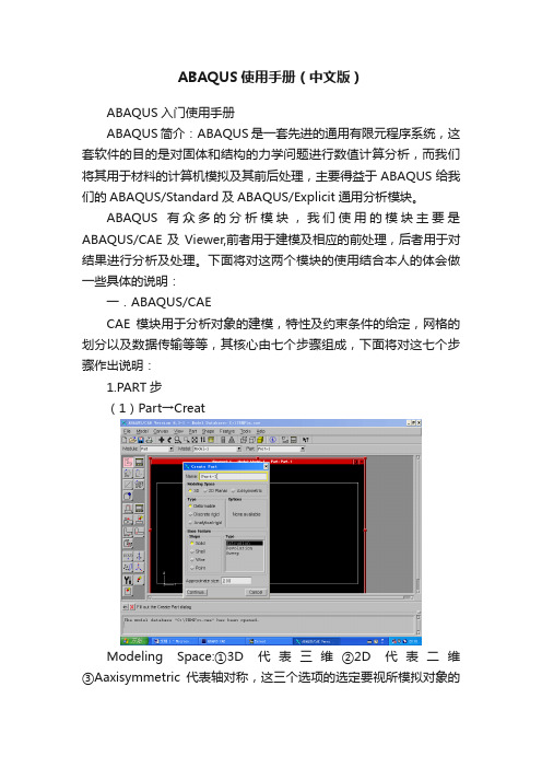
下面将对这两个模块的使用结合本人的体会做一些具体的说明:一.ABAQUS/CAECAE模块用于分析对象的建模,特性及约束条件的给定,网格的划分以及数据传输等等,其核心由七个步骤组成,下面将对这七个步骤作出说明:1.PART步(1)Part→CreatModeling Space:①3D代表三维②2D代表二维③Aaxisymmetric代表轴对称,这三个选项的选定要视所模拟对象的结构而定。
Type: ①Deformable为一般选项,适合于绝大多数的模拟对象。
②Discrete rigid 和Analytical rigid用于多个物体组合时,与我们所研究的对象相关的物体上。
ABAQUS假设这些与所研究的对象相关的物体均为刚体,对于其中较简单的刚体,如球体而言,选择前者即可。
若刚体形状较复杂,或者不是规则的几何图形,那么就选择后者。
需要说明的是,由于后者所建立的模型是离散的,所以只能是近似的,不可能和实际物体一样,因此误差较大。
Shape中有四个选项,其排列规则是按照维数而定的,可以根据我们的模拟对象确定。
Type: ①Extrusion用于建立一般情况的三维模型②Revolution建立旋转体模型③Sweep用于建立形状任意的模型。
Approximate size:在此栏中设定作图区的大致尺寸,其单位与我们选定的单位一致。
设置完毕,点击Continue进入作图区。
(word完整版)Abaqus基本操作中文教程(2021年整理精品文档)

(word完整版)Abaqus基本操作中文教程(word完整版)Abaqus基本操作中文教程编辑整理:尊敬的读者朋友们:这里是精品文档编辑中心,本文档内容是由我和我的同事精心编辑整理后发布的,发布之前我们对文中内容进行仔细校对,但是难免会有疏漏的地方,但是任然希望((word完整版)Abaqus基本操作中文教程)的内容能够给您的工作和学习带来便利。
同时也真诚的希望收到您的建议和反馈,这将是我们进步的源泉,前进的动力。
本文可编辑可修改,如果觉得对您有帮助请收藏以便随时查阅,最后祝您生活愉快业绩进步,以下为(word完整版)Abaqus基本操作中文教程的全部内容。
(word完整版)Abaqus基本操作中文教程Abaqus基本操作中文教程(word完整版)Abaqus基本操作中文教程目录1 Abaqus软件基本操作 (4)1.1 常用的快捷键 (4)1。
2 单位的一致性 (4)1。
3 分析流程九步走 (5)1。
3。
1 几何建模(Part) (5)1.3。
2 属性设置(Property) (7)1。
3。
3 建立装配体(Assembly) (7)1.3.4 定义分析步(Step) (9)1。
3.5 相互作用 (Interaction) (10)1。
3.6 载荷边界(Load) (13)1。
3。
7 划分网格 (Mesh) (14)1.3。
8 作业(Job) (18)1.3.9 可视化(Visualization) (19)(word完整版)Abaqus基本操作中文教程1 Abaqus软件基本操作1.1 常用的快捷键旋转模型— Ctrl+Alt+鼠标左键平移模型 - Ctrl+Alt+鼠标中键缩放模型 - Ctrl+Alt+鼠标右键1.2 单位的一致性CAE软件其实是数值计算软件,没有单位的概念,常用的国际单位制如下表1所示,建议采用SI (mm)进行建模。
国际单位SI (m)SI (mm)制长度m mm力N N质量kg t时间s sPa应力MPa (N/mm2)(N/m2)质量密度kg/m3t/mm3加速度m/s2mm/s2例如,模型的材料为钢材,采用国际单位制SI (m)时,弹性模量为2。
ABAQUS Tutorial - Debond 步骤
编辑截面如下图,厚度 10,单击 OK
-4-
Vehicle
10. 单击
, 并在
中的 part
下拉菜单中选中 upper。然后点击绘图框中的图形实体,赋予截面,并完成下图对话框,默认设 置,单击 OK
11. 重复 10 步,part 下拉菜单中选中 lower,其余与 10 步相同。 12. 赋予材料截面属性后, 进入 assembly 模块, 单击 选择 independent 并点击 OK 退出。 , 建 立 instance, 同时选中 upper 和 lower,
选择最下端平面为约束面,如图。
- 11 -
Vehicle
22. 进入 step 模块,建立 step-1,默认设置,continue
Nlgeom 设置为 on 其余默认,ok 退出。
23. 进入 load 模块,建立 step-1 下的 pressure,-108,OK 退出
- 12 -
Vehicle
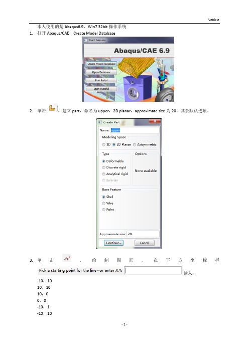
形
,
在
下
方
坐 输入:
标
栏
-10,10 10,10 10,0 0,0 -10,1 -10,10
-1-
Vehicle
完成如下图图形,单击中键确认退出。
4. 再单击
,建立一个新的 part,命名为 lower,其余与 2 步相同。
5. 与 3 步相同,输入坐标: -10,-10 10,-10 10,0 0,0 -10,-1 -10,-10 完成如下图形,单击中键确认退出。
其余默认,OK 退出。
-6-
Vehicle
16. 单击
,同时选中 upper 和 lower,确认后得到网格如下。
17. 进入 interaction 模块,
ABAQUS_plane_stress_tutorial
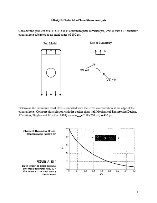
ABAQUS Tutorial – Plane Stress AnalysisConsider the problem of a 4” x 2” x 0.1” aluminum plate (E=10e6 psi, ν=0.3) with a 1” diameter circular hole subjected to an axial stress of 100 psi.Determine the maximum axial stress associated with the stress concentration at the edge of the circular hole. Compare this solution with the design chart (ref. Mechanical Engineering Design, 5th edition, Shigley and Mischke, 1989) value σmax = 2.18 (200 psi) = 436 psi.Use of SymmetryFull ModelFinite Element solution (ABAQUS)Start => Programs => ABAQUS 6.5-1 => ABAQUS CAESelect 'Create Model Database'File => Save As => create directory for filesModule: SketchSketch => Create => Approx size - 5Add=> Point => enter coordinates (.5,0), (1,0), (1,2), (0,2), (0,.5) => select 'red X'View => Auto-FitAdd => Line => Connected Line => select point at (.5,0) with mouse, then (1,0), (1,2), (0,2), (0,.5) => right click => Cancel Procedure => DoneAdd => Arc => Center/Endpoint => select point at (0,0), then (.5,0), then (0,.5) => Cancel Procedure => DoneModule: PartPart => Create => select 2D Planar, Deformable, Shell, Approx size - 5=> ContinueAdd => Sketch => select 'Sketch-1' => Done => DoneModule: PropertyMaterial => Create => Name: Material-1, Mechanical, Elasticity, Elastic => set Young's modulus = 10e6, Poisson's ratio = 0.3 => OKSection => Create => Name: Section-1, Solid, Homogeneous => Continue => Material - Material-1, plane stress/strain thickness - 0.1 => OKAssign Section => select entire part by dragging mouse => Done => Section-1 => OK Module: AssemblyInstance => Create => Part-1 => OKModule: StepStep => Create => Name: Step-1, Initial, Static, General => Continue => nlgeom off => OK Module: LoadLoad => Create => Name: Step-1, Step: Step 1, Mechanical, Pressure => Continue => select top edge => Done => set Magnitude = -100 => OKBC => Create => Name: BC-1, Step: Step-1, Mechanical, Symmetry/Antisymmetry/Encastre => Continue => select bottom edge => Done => YSYM (U2=UR1=UR2=0)BC => Create => Name: BC-2, Step: Step-1, Mechanical, Symmetry/Antisymmetry/Encastre => Continue => select left edge => Done => XSYM (U1=UR2=UR3=0)Module: MeshSeed => Edge by Size => select full model by dragging mouse => Done => Element Size=0.1 => press Enter => DoneMesh => Controls => Element Shape => Tri (for triangles), Quad (for quadrilaterals), or Quad dominated (for mixed triagles and quads - mostly quads)Mesh => Element Type => Plane Stress => Linear/Tri (for CST), Quadratic/Tri (for LST), Linear/Quad (for 4 node quad), or Quadratic/Quad (for 8-node quad) => OK => Done Mesh => Instance => OK to mesh the part Instance: Yes => DoneTools => Query => Region Mesh => Apply (displays number of nodes and elements at bottom of screen)Module: JobJob => Create => Name: Job-1, Model: Model-1 => Continue => Job Type: Full analysis, Run Mode: Background, Submit Time: Immediately => OKJob => Manager => Submit => Job-1ResultsModule: VisualizationPlot => Deformed ShapeDeformed Shape Options => Basic => Show superimposed undeformed plot => OKView => Graphics Options => Background Color => WhiteCtrl-C to copy viewport to clipboard => Open MS Word Document => Ctrl-V to paste image Plot=> Contours => Result => Option => Set Nodal Averaging Threshold to 0% => Apply Result => Field Output => Name - S => Component = S22 => OKContour Options => Limits => Specify Max = 450, Min = 0 => OKCtrl-C to copy viewport to clipboard => Open MS Word Document => Ctrl-V to paste image Tools => Query => Probe Values => Apply => select desired Field Output (S11, S22, etc.) => Probe Nodes => move cursor to desired location to view nodal resultsTools => Path => Create => Node List => Continue => Add Before => select nodes along bottom edge => Done => OKTools => XY Data => Create Path => Continue => X Distance => PlotCtrl-C to copy viewport to clipboard => Open MS Word Document => Ctrl-V to paste image Report => Field Output => Setup => Number of Significant Digits => 6Report => Field Output => Position - Centroid => Variable - S => ApplyExamine tabulated results in 'abaqus.rpt' file.Mesh Convergence study:Repeat procedure for various mesh densities and element types (CST, LST, 4-node Quad and 8-node Quad). Also, refine mesh locally near stress concentration at the edge of the holeusing "Seed - Edge Biased" in Mesh Module.Effect of Element Type and Mesh DensityTo evaluate the performance of several element types and to examine the effects of meshrefinement, consider the following 8 cases:* Coarse mesh = 5 elements along each edge,Medium mesh = 10 elements along each edge,Fine mesh = 25 elements along each edgeResultsThe cases described above were run using ANSYS. ABAQUS is expected to provide identical results.。
Abaqus教程
Table of Figures
Figure 1. Dimensions and loading of composite plate .................................................................................. 3 Figure 2. Plate dimensions............................................................................................................................ 5 Figure 3. Helius:MCT GUI ............................................................................................................................. 7 Figure 4. Edit Composite Layup dialog box .................................................................................................. 9 Figure 5. Ply-1 orientation ........................................................................................................................... 10 Figure 6. Shell Parameters ......................................................................................................................... 11 Figure 7. Edit Step dialog box ..................................................................................................................... 13 Figure 8. Edit Field Output Request dialog box .......................................................................................... 14 Figure 9. Location (red) of bottom surface boundary condition .................................................................. 15 Figure 10. Location of top surface (red) load boundary condition .............................................................. 16 Figure 11. Element hourglass stiffness settings ......................................................................................... 18 Figure 12. Plate mesh ................................................................................................................................. 19 Figure 13. Edit keywords dialog box ........................................................................................................... 20 Figure 14. Failure plot of ply 1 at the end of the step ................................................................................. 22 Figure 15. Envelope plot of SDV1 at the end of the step............................................................................ 23
ABAQUS tutorial

EN175: Advanced Mechanics of SolidsDivision of EngineeringBrown UniversityABAQUS tutorial1. What is ABAQUS?ABAQUS is a highly sophisticated, general purpose finite element program, designed primarily to model the behavior of solids and structures under externally applied loading. ABAQUS includes the following features:Capabilities for both static and dynamic problemsThe ability to model very large shape changes in solids, in both two and threedimensionsA very extensive element library, including a full set of continuum elements,beam elements, shell and plate elements, among others.A sophisticated capability to model contact between solidsAn advanced material library, including the usual elastic and elastic – plasticsolids; models for foams, concrete, soils, piezoelectric materials, and many others.Capabilities to model a number of phenomena of interest, including vibrations,coupled fluid/structure interactions, acoustics, buckling problems, and so on.The main strength of ABAQUS, however, is that it is based on a very sound theoretical framework As an practicing engineer, you may be called upon to make crucial decisions based on the results of computer simulations. While no computer program can ever be guaranteed free of bugs, ABAQUS is among the more trustworthy codes. Furthermore, as you will see if you consult theABAQUS theory manual, HKS developers really understand continuum mechanics (since many of them are Brown Ph.Ds, this goes without saying). For this reason, ABAQUS is used by a wide range of industries, including aircraft manufacturers, automobile companies, oil companies and microelectronics industries, as well as national laboratories and research universities.ABAQUS is written and maintained by Hibbitt, Karlsson and Sorensen, Inc (HKS), which has headquarers in Pawtucket, RI. The company was founded in 1978 (by graduates of Brown’s Ph.D. program in solid mechanics), and today has several hundred employees with offices around the world.2. Tutorial OverviewIn this tutorial, you will learn how to run ABAQUS/Standard, and also how to useABAQUS/Post to plot the results of a finite element computation.First, you will use ABAQUS to solve the following problem. A thin plate, dimensions, contains a hole of radius 1cm at its center. The plate is made fromsteel, which is idealized as an elastic—strain hardening plastic solid, with Young’s modulusE=210GPa and Poisson’s ratio . The uniaxial stress—strain curve for steel isidealized as a series of straight line segments, as shown below.The plate is loaded in the horizontal direction by applying tractions to its boundary.The magnitude of the loading increases linearly with time, as shown.You may recall that a circular hole in a plate has a stress concentration factor of about 3. At time t=1, therefore, the stress at point A should just reach yield (the initial yield stress of the plate is 200MPa). At time t=3, the load should be enough to cause a significant portion of the plate to yield.We will specifically request ABAQUS to print the state of the solid at time t=1, t=2 andt=3, to see the development of plasticity in the plate.Observe that the plate and the loading is symmetrical about horizontal and vertical axes through the center of the plate. We only need to model ¼ of the plate, therefore, and can apply symmetry boundary conditions on the the bottom and side boundaries. The finite element mesh you will use for your computations is shown below. The elements are plane stress, 4 noded quadrilaterials. Symmetry boundary conditions are applied as shown, and distributed tractions are applied to the rightmost boundary.The ABAQUS input file that sets up this problem will be provided for you. You will run ABAQUS, and then use ABAQUS/Post to look at the results of your analysis. Next, youwill take a detailed look at the ABAQUS input file, and start setting up input files of yourown. After completing this tutorial, you should be in a position to do quite complex two andthree dimensional finite element computations with ABAQUS, and will know how to viewthe results. We will continue using ABAQUS to solve various problems throughout the restof this course.3. Steps in running ABAQUSCreate an input file. ABAQUS works by reading and responding to a set of commands(called KEYWORDS) in an input file. The keywords contain the information to define the mesh, the properties of the material, the boundary conditions and to control output from the program. To see the ABAQUS input file for the plate problem, click here.Run the program. On Windows NT, ABAQUS is controlled by typing commands into aDOS type window.Post processing. There are two ways to look at the results of an ABAQUS simulation. You can ask the program to print results to a file, which you can look at with a text editor. This is painful… Alternatively, you can use a program called ABAQUS/Post, which can be used to plot various quantities that may be of interest.We will begin this tutorial by running through all these stages with a pre-existing input file, then look in more detail at how to set up an input file.BEFORE RUNNING ABAQUS FOR THE FIRST TIME:1. Open an MS/DOS window on your workstation (the command to openthe window is located in the Start menu on your toolbar).2. Type mk_ABAQUS in the MS/DOS window. If the commandexecutes correctly, icons to start ABAQUS and to open the ABAQUSdocumentation should appear on your desktop. In addition, a directorycalled ABAQUS should be created in your home directory.4. Downloading the sample ABAQUS input file.1. If you completed the preceding step correctly , a directory called ABAQUS shouldhave been created in your home directory. Within your ABAQUS directory, create a subdirectory called tutorial to store your input files and results. ABAQUS will generatea vast number of output files, and to keep track of them, it is convenient to keep all the filesassociated with a particular problem in one directory.2. Download the example ABAQUS file. To do so, click here. You will see the input fileappear in the frame. Click anywhere on the frame, then select Save Frame As… from the File menu on the top left hand corner of your browser. In the popup window, find thedirectory called ABAQUS\tutorial , and save the file as tutorial.inp3.Open tutorial.inp with a text editor. Take a quick look at the file and make sure that itdownloaded correctly.4. Exit the text editor.In future, you will create your own ABAQUS input file, by typing in appropriate keywords with a text editor. The easiest thing to do will be to copy an existing file, and modify it for other problems.5. Running ABAQUS.1. Double click the ABAQUS icon on your desktop. A window with a black backgroundshould appear.2. In the Abaqus Command window, change directories to ABAQUS\tutorial.3. In the Abaqus Command window, typeYour Prompt > abaqus [return]Identifier: tutorial [return]User routine file: [return](The identifier should always be the name of the .inp file, without the .inp extension. The user routine file will always be blank in anything we run in this course. It is needed onlywhen you start to write your own subroutines to run within ABAQUS). This starts theABAQUS program running. Note that the program runs in the background, so although the prompt comes right back in the ABAQUS window, this does not mean the program hasfinished. Note also that some special computations (e.g. using the *SYMMETRIC MODEL GENERATION key) will cause ABAQUS to ask you some more questions duringexecution.4. Using explorer, or by opening a directory window, examine the files in the directorytutorial. (Click here if you don’t know how to do this). You should see the following files: tutorial.inptutorial.dattutorial.logtutorial.restutorial.battutorial.statutorial.msgtutorial.filFortunately, you can happily ignore most of these files. The only ones you need to look at are tutorial.log, tutorial.sta, tutorial.msg and tutorial.dat. We will also use tutorial.res and tutorial.fil later.5. Open the file called tutorial.log with a text editor. You will see some information aboutthe time it took to for ABAQUS to complete execution. You should also see that the fileends withABAQUS JOB tutorial COMPLETEDThis means that ABAQUS is done and you can safely look at the results.6. Open the file called tutorial.sta with a text editor. You will see columns of numbers, headed bySUMMARY OF JOB INFORMATION:STEP INC ATT SEVERE EQUIL TOTAL TOTAL STEP INC OF DOF IFDISCON ITERS ITERS TIME/ TIME/LPF TIME/LPF MONITOR RIKSITERS FREQThis file is continuously updated by ABAQUS as it runs, and tells you how much of the computation has been completed. You can monitor this file while ABAQUS is running. We will discuss the meaning of data in this file in more detail later.7. Open the file called tutorial.dat. This file contains all kinds of information about the computations that ABAQUS has done. In particular, if ABAQUS encounters any problems during the computation, error and warning messages will be written to this file. You should first check the end of the file to see if the computation was successful. If the program ran successfully, you should see a message sayingANALYSIS COMPLETEWITH 7 WARNING MESSAGES ON THE MSG FILEJOB TIME SUMMARYUSER TIME (SEC) = 20.000SYSTEM TIME (SEC) = 3.0000TOTAL CPU TIME (SEC) = 23.000WALLCLOCK TIME (SEC) = 36The times listed above may differ on your computer, depending on the speed of theprocessor and the memory available. The warning message is a bit scary, but is actuallynothing to worry about. We’ll see why it appears later.You can explore the rest of this file to see what else is there. MAKE SURE YOU CLOSE THE FILE BY EXITING THE TEXT EDITOR BEFORE PROCEEDING.6. ABAQUS ERRORS1. Next, we will deliberately introduce an error into the ABAQUS input file tutorial.inp, tosee what an unsuccessful run looks like. Open the file tutorial.inp with a text editor, andchange the line near the top that says*RESTART, WRITE, FREQ=1 to*RESTART, WONK, FREQ=1 Save the file in Text Only format. Now, repeat step 3 in Running ABAQUS to runABAQUS again. You will get an additional prompt as follows.Old job files exist. Overwrite (y/n)? : y [return]2. Check the files in the directory ABAQUS\tutorial again. This time, not all the files willbe there, because the run was unsuccessful.3. Open the file called tutorial.log with a text editor. Note the error message there.4. Open the file called tutorial.dat with a text editor. You will see that the end of the filecontains the following statementsTHE PROGRAM HAS DISCOVERED 3 FATAL ERRORS** EXECUTION IS TERMINATED **END OF USER INPUT PROCESSINGJOB TIME SUMMARYUSER TIME (SEC) = 0.0000SYSTEM TIME (SEC) = 0.0000TOTAL CPU TIME (SEC) = 0.0000WALLCLOCK TIME (SEC) = 2This again shows that ABAQUS ran into trouble during execution. Search the file backwards for the occurrence of ERROR to find the lines***ERROR: UNKNOWN PARAMETER WONKCARD IMAGE: *RESTART, WONK, FREQ=1***NOTE: DUE TO AN INPUT ERROR THE ANALYSIS PRE-PROCESSOR HAS BEEN UNABLE TOINTERPRET SOME DATA. SUBSEQUENT ERRORS MAY BE CAUSED BY THIS OMISSION***ERROR: EITHER THE PARAMETER READ OR WRITE MUST BE SPECIFIEDCARD IMAGE: *RESTART, WONK, FREQ=1***ERROR: PARAMETER FREQUENCY IS ONLY MEANINGFUL IF THE WRITE PARAMETER IS ALSO SPECIFIEDCARD IMAGE: *RESTART, WONK, FREQ=1This will tell you what part of the input file is causing problems, and if you are lucky, you will understand the error message. Notice that ABAQUS programmers still seem to beusing punch cards. ABAQUS is coded in FORTRAN, too (for real).5. Try another error. Change the line*RESTART, WONK, FREQ=1 back to*RESTART, WRITE, FREQ=1 This time, change the line1031, 5.E-02, 5.E-02to1031, 5.E-02, -5.E-02Re-run ABAQUS (don’t forget to save the .inp file first), then check the file tutorial.datagain. ABAQUS really freaks out with this problem. You should see 96 fatal errors. If you have no life, you might like to try and see if you can produce more errors than this byinserting a single character in the input file.6. Before proceeding, correct the input file, and re-run ABAQUS. Check the .dat file and.log file to make sure that the job ran properly.7. Running ABAQUS/Post.1. If you have not already done so, run ABAQUS with a correct input filetutorial.inp. You can download an error free copy of the tutorial file by clicking hereif you need to.2. To run ABAQUS/Post, you will need to start a program called Exceed first. FindExceed on the Start menu of your desktop, and select it to start it running. A windowwill be displayed briefly and an icon should appear on your toolbar if the programstarted properly.3. Make sure you have an ABAQUS command window open, set to the appropriatedirectory. In the ABAQUS command window, typeabaqus post4. A window should appear, which will be used to display results of the ABAQUSrun. To do so, you type commands in the bottom left hand corner of the window. Wewill try a few useful commands in the next section8. Online help with ABAQUS/PostIn the ABAQUS/Post window, typehelp [return]A black window will open, with a list of ABAQUS/Post commands. To get helpwith any command, just type the command name.9. ABAQUS/Post Mesh and Boundary Condition Display1.The first step is to read the results of an analysis into ABAQUS/Post. Our examplesimulation created two files that can be read into ABAQUS/Post:tutorial.restutorial.filThe file named tutorial.res is called a `restart file’ (the file always has .resextension). This file contains full information about the analysis. The restart file ismost useful if you want to plot the finite element mesh, or contours of stress, displacement, etc. The file named tutorial.fil is called a `results file’ (the file always has a .fil extension). This file contains data that were specifically requested in the ABAQUS input file. The results file is most useful when you want to create x-y plots of stress-v-time, stress-v-strain, or similar.To read the restart file, typerestart, file=tutorial [return]A black window will pop up, with lots of interesting information in it. Ignore the useful information and type [return] anywhere in the window. When you read the restart file with this syntax, all quantities displayed will represent the state of the solid at the very end of the analysis. We will see how to display data at other times lower down.2. Now, we can start plotting things. Typedraw [return]in the ABAQUS/Post window. This will plot the undeformed finite element mesh.3. To display node numbers with the mesh, typeset, n numbers=on [return]draw [return]4. To display element numbers with the mesh, typeset, el numbers=on [return]draw [return]5. To zoom in and out of the mesh, right click on the mesh and drag the mouse left or right, while continuing to hold the mouse button down.6. To move the mesh around on the window, center click on the mesh and drag the mouse.7. To rotate the FEM mesh, left click and drag the mouse, and/or left click with the shift key held down while dragging the mouse. (This is not too helpful with a 2D mesh, but is very useful in 3D).8. Another useful way to zoom in on a small region iszoom, cursor [return]Now, click on the mesh at two points. The two points define opposite corners of a box. When you typedraw [return]the region within the box will be scaled to fit the full window.9. To turn off element numbers and node numbers again, typeset, el numbers=off, n numbers=off [return]draw [return]10. To get back to the original view of the mesh, typereset, all [return]draw [return]11. Another useful option for checking a mesh isset, fill=on [return]draw [return]report elements [return]Now, click on any element in the mesh, and information concerning the element will be displayed at the bottom of the window. To exit this option, click on the little X at the bottom left hand corner of the black window. The keyreport nodes [return]tells you about nodes.12. You can also display the boundary conditions applied to the mesh, by typingset, bc display=ondrawIf you have superb eyesight, you will see some little dots on the left and bottomedges of the mesh. Zoom in, and you will see arrows representing the constraintsapplied to the bottom of the mesh.13. Before proceeding to the next section, typereset, all [return]10. ABAQUS/Post Field PlotsIf you have not already done so, start up ABAQUS/Post and read in tutorial.res1. To view the deformed shape of the solid after loading, typedraw, displaced [return]You can use the mouse to drag the mesh away from the text message that appears onthe window. Note that the deformation is grossly exaggerated to show it clearly: thescale factor is displayed on the text message.2. Recall that, by default, ABAQUS/Post will display the state of the solid at thevery end of whatever load history was specified in the input file. To see the results atother times, you can typerestart, step=1 [return]draw, displaced [return]This will display the deformed mesh at the end of the first load step. In this case, thedeformed mesh doesn’t look very different at the end of the first step, but you shouldsee a message in the bottom left hand corner of the screen telling you that the currentstep is 1.3. To remove the undeformed mesh, typeset, undeformed=off [return]draw, displaced [return]4. To see the actual displacements (without magnification), typeset, d magnification=1.0 [return]draw, displaced [return]5. To plot a contour of the horizontal component of stress , typecontour, v=s11 [return]6. To show the contours as solid colors instead of lines, typeset, fill=on [return]contour, v=s11 [return]7. To remove the mesh to see the contours more clearly, typeset, outline=perimeter[return] or set, outline=off [return]contour, v=s11 [return]8. To turn the mesh back on again, typeset, outline=element [return]9. You can plot all field quantities the same way. Examples includev=s22; v=s12, v=s33, etc plot various stress componentsv=mises plots von Mises stress.10. You can do vector plots too. For examplevector plot, v=u [return]shows arrows whose length and orientation correspond to the vector displacement at each node. Obviously, you can only do a vector plot of a vector valued function…11. You can also display numerical values of variables (stress, displacements, etc) at nodes or integration points (whichever applies) by typingreport values, v=s11 [return]Then, click with the mouse on any element. Values of stress at each elementintegration point will be printed at the bottom of the screen. To exit this option, clickon the little cross at the bottom left hand corner of the black window. To seedisplacements, typeReport values, v=u1 [return]Then, click on any node to see the horizontal component of displacement there.11. ABAQUS STEPS AND INCREMENTSYou may have noticed when reading the restart file that ABAQUS was telling youwhich step was being read, and which increment. This is somewhat mysterious, sowe will explore how ABAQUS controls time during an analysis next.When you set up an ABAQUS/Standard input file, you tell ABAQUS to apply loadto a solid in a series of steps. For the hole in a plate problem, we applied load to thesolid in three steps, from t=0 to t=1 (step 1); from t=1 to t=2 (step 2) and finallyfrom t=2 to t=3. ABAQUS will always print out the state of the solid at the end ofeach step. When you type restart, step=2in ABAQUS/Post and then plotsomething, you will see the state of the solid at the end of step 2 – in this case, at time t=2.Let’s check this out. We will compare the plastic zone size in the solidat times t=1, t=2 and t=3.1. If you have not already done so, start up ABAQUS/Post, and read intutorial.res.2. Now, we will open up three windows to display all three times onthe same picture. Typewindow, name=first, maximum=(0.4,1.0),minimum=(0.0,0.6) [return]window, name=second, maximum=(0.7,0.7),minimum=(0.3,0.3) [return]window, name=third, maximum=(1.0,1.0),minimum=(0.6,0.6) [return]Here, the maximum=… specifies the coordinates of the upper righthand corner of the window, while the minimum specifies the lowerleft hand corner. You can also use window, name=..., cursor and thenclick on the screen with the mouse to define the corners of thewindow, but don’t try that now or else you will have an extra windowopen that you don’t want.3. Now, we will plot contours of plastic strain at t=1¸t=2 and t=3 inthe three windows. Typewindow, name=first [return]set, fill=on [return]restart, step=1 [return]contour, v=pemag [return]window, name=second [return]restart, step=2 [return]contour, v=pemag [return]window, name=third [return]restart, step=3 [return]contour, v=pemag [return]You should see three contour plots at the end, showing plastic straincontours. The deep blue color is the contour level for zero plasticstrain, showing areas that have not yet yielded. The red color has thehighest plastic strains. In the first window, there will only be a smallplastic zone at the edge of the hole. This plastic zone grows as the loadis increased. You can see this in the other two windows. On the thirdwindow, most, but not quite all, of the plate has started to deformplastically.So, what’s the deal with the increments? Well, because the plate isdeforming plastically, this is a nonlinear problem – the stress is anonlinear function of the nodal displacements. This means thatABAQUS needs to iterate to find the correct solution (a Newton-Raphson iteration is used to solve the nonlinear equilibriumequations), and also means that ABAQUS cannot accurately computethe plastic strain that results from a large change in loads. Indeed, ifABAQUS tries to take a very large time step, it may not be able tofind a solution at all.To get around this problem, ABAQUS automatically subdivides alarge time step into several smaller `increments’ if it finds that thesolution is nonlinear. This process is completely automatic, andABAQUS will always take the largest possible time increments thatwill reach the end of the step and still give an accurate, convergentsolution. You don’t know a priori how many increments ABAQUSwill take.You can find out, however, by looking at some of the output files. Youcan look at tutorial.sta, for example which shows the followinginformation:SUMMARY OF JOB INFORMATION:STEP INC ATT SEVERE EQUIL TOTAL TOTAL STEP INC OF DOF IFDISCON ITERS ITERS TIME TIME TIME MONITOR RIKS1 1 1 0 4 4 1.00 1.00 1.0002 1 2 0 4 4 1.25 0.250 0.25002 2 1 03 3 1.50 0.500 0.25002 3 1 0 4 4 1.88 0.875 0.37502 4 1 0 4 4 2.00 1.00 0.12503 1 3 0 5 5 2.06 0.0625 0.062503 2 1 0 3 3 2.13 0.125 0.062503 3 1 0 3 3 2.19 0.188 0.062503 4 1 0 3 3 2.28 0.281 0.093753 5 1 0 3 3 2.42 0.422 0.14063 6 1 04 4 2.63 0.633 0.21093 7 1 04 4 2.95 0.949 0.31643 8 1 0 1 1 3.00 1.00 0.05078This file is continually updated and can be monitored during and ABAQUS computation. The first column shows which step ABAQUS is currently analyzing. The second column shows which time increment ABAQUS has reached. The seventh column shows the current time.From this information, we learn that the first step was completed in one increment (this is because the plate did not reach yield until the end of the increment, so very large time steps could be taken). The second step was completed in four increments, and the third step was completed in 8 increments.The file named tutorial.msg contains much more information concerning the increments used, the iterative process, and the tolerances that ABAQUS has applied to determine whether a solution has converged. You need a Ph.D to be able to figure most of that stuff out. We can see the meaning of the warning messages that were referred to in the .dat file, however – every time ABAQUS has to reduce the time increment due to convergence problems, a warning message is printed to the .msg file. This is nothing to worry about – everything is working perfectly.ABAQUS prints information concerning the state of the solid to the .res and .fil files at the end of each increment.4. To go back to a single window, typewindow, remove=all [return]4. To look at the plastic zone at time t=2.42 (step 3, increment 5), typerestart, step=3, increment=5 [return]contour, v=pemag [return]12. ABAQUS/Post X-Y PlotsABAQUS/Post can also be persuaded to plot variations of stress, displacement, etcwith position within the solid, or can display stresses, strains, etc as a function oftime at a point in the solid, or can even plot stress as a function of strain (or anythingelse, for that matter). The procedure to do this is rather weird.We will begin by plotting x-y graphs of field quantities with position in the solid.If you have not already done so, start up ABAQUS/Post and read in tutorial.res.1. First, we will plot the variation of with distance along the base.First, we define a set of data known as a `curve,’ by using the path keywordpath, node list, variable=s22, name=syy, distance, absolute [return]>119 [return]>120 [return]>121 [return]… Continue typing in numbers in increasing order until you get to>131 [return]>[return]This procedure defines a set of (x,y) data pairs at each node entered in the list. The xcoordinate is zero at the first node, and is incremented by the distance between nodesfor each subsequent node in the list. The y coordinate is s22.The group of all the data pairs generated by this command has been given the name`syy’. To find the list of nodes you need for the path of interest, it is simplest to plotthe mesh with node numbers.2. Now, we can plot these (x,y) data pointsdisplay curve [return]> syy [return]> [return]3. We can define and plot other data on the same graph. Instead of typing in a list of nodes this time, we will use the `generate’ key to generate the list automatically path, node list, generate, variable=s11, name=sxx, distance, absolute [return] >119,131,1 [return]>[return]display curve [return]> syy [return]> sxx [return]> [return]Do you see anything wrong with the value of sxx at x=0? Why? What could cause this error?4. For a 3D analysis, you can ask for curves to be generated along a straight line, instead of entering a list of node numbers. To produce the results we want here, we would enterpath, start=(0.01,0.0), end=(0.05,0.0), variable=s22, name=syy,distance, absolute [return]Unfortunately, this does not work in 2D, so you are stuck entering node lists.5. There are various commands you can use to change the appearance of the x-y plot. For examplegraph axes, x title=x, y title=normal stress, x grid=solid, y grid=solid [return] display curve [return]>syy [return]> [return]Unfortunately, no matter how hard you try, x-y plots output from ABAQUS/Post look pretty shitty. If you want publication quality output, your best bet is to print the data and plot it with something else, or print out a postscript file and then edit it with another graphics package.6. The path defined by the node list need not be a straight line. For example, to plot the variation of Mises stress around the perimeter of the hole, usepath, node list, generate, variable=mises, name=sm, distance, absolute [return]。
《Abaqus教程》课件

06
Abaqus未来发展与展望
人工智能与机器学习在Abaqus中的应用
预测模型
利用机器学习技术,对Abaqus模拟结果进行预测 ,提高预测精度。
自动化优化
结合人工智能算法,实现Abaqus模型的自动优化 ,提高设计效率。
自动化校准
利用机器学习技术,自动校准Abaqus模型的参数 ,减少人工干预。
标准化接口
推动Abaqus的标准化接口发展,促进软件之间的互操作性。
THANKS FOR WATCHING
感谢您的观看
接触表面处理
在进行接触设置时,需要对接触表面进行处理,如 粗糙度、摩擦系数等,以确保模拟结果的准确性。
接触条件
在模拟过程中,用户需要设定接触条件,如 接触压力、温度等,以控制模拟的边界条件 。
优化设计
优化目标
用户可以根据实际需求设定优化目标,如最小化重量、最大化刚度 等,以实现结构优化设计。
优化算法
02
Abaqus基本操作
启动与退
启动Abaqus
打开Abaqus软件,选择合适的模块 和许可证。
退出Abaqus
完成操作后,选择“文件”菜单中的 “退出”选项,保存更改并关闭软件 。
模型创建
创建模型
在“模型”菜单中选择“创建模型”选项,选择合适的单位和坐标系。
创建部件
在“模型”菜单中选择“创建部件”选项,输入部件名称和尺寸。
材料模型的发展与挑战
01
02
03
新材料模型
随着新材料的发展,需要 开发新的材料模型以适应 模拟需求。
多物理场耦合
实现多物理场(如热、力 、电等)的耦合模拟,提 高模拟精度。
参数的不确定性
Abaqus_Vibrations_Tutorial
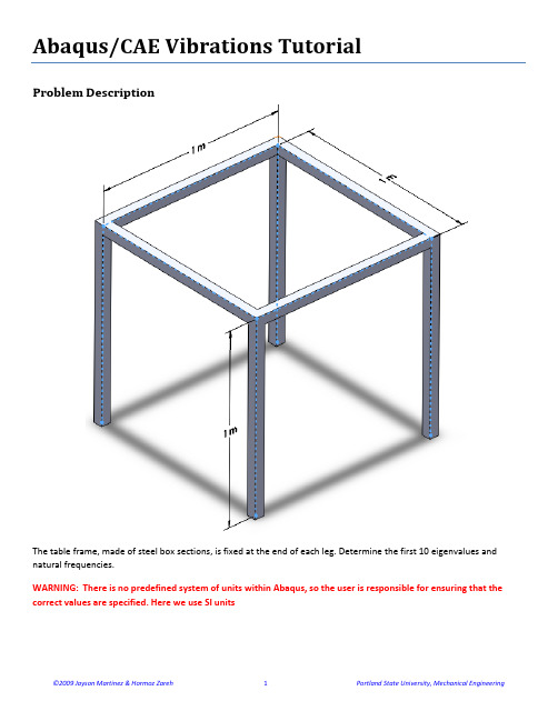
Abaqus/CAE Vibrations TutorialProblem DescriptionThe table frame, made of steel box sections, is fixed at the end of each leg. Determine the first 10 eigenvalues and natural frequencies.WARNING: There is no predefined system of units within Abaqus, so the user is responsible for ensuring that the correct values are specified. Here we use SI unitsAnalysis Steps1.Start Abaqus and choose to create a new model database2.In the model tree double click on the “Parts” node (or right click on “parts” and select Create)3.In the Create Part dialog box (shown above) name the part anda.Select “3D”b.Select “Deformable”c.Select “Wire”d.Set approximate size = 5 (Not important, determines size of grid to display)e.Click “Continue…”f.Create the sketch shown below4.In the toolbox area click on the “Create Datum Plane: Offset From Principle Plane” icona.Select the “XY Plane” and enter a value of 1 for the offset5.In the toolbox area click on the “Create Wire: Planar” icona.Click on the outline of the datum plane created in the previous stepb.Select any one of the lines to appear vertical and on the rightc.In the toolbox area click on the “Project Edges” icond.Select all of the lines in the viewport and click “Done”6.In the toolbox area click on the “Create Datum Plane: 3 points” icon (click on the small black triangle in thebottom‐right corner of the icon to get all of the datum plane options)a.Select 3 points on the top of the geometry7.In the toolbox area click on the “Create Wire: Planar” icona.Click on the outline of the datum plane created in the previous stepb.Select any one of the lines to appear vertical and on the rightc.Sketch two lines to connect finish the wireframe of the tabled.Click on “Done”8.Double click on the “Materials” node in the model tree the new material and give it a descriptionb.Click on the “Mechanical” tabÎElasticityÎElasticc.Define Young’s Modulus (210e9) and Poisson’s Ratio (0.25)d.Click on the “General” tabÎDensitye.Density = 7800f.Click “OK”9.Double click on the “Profiles” node in the model tree the profile and select “Box” for the shapeb.Click “Continue…”c.Enter the values for the profile shown belowd.Click “OK”10.Double click on the “Sections” node in the model tree the section “BeamProperties” and select “Beam” for both the category and the typeb.Click “Continue…”c.Leave the section integration set to “During Analysis”d.Select the profile created above (BoxProfile)e.Select the material created above (Steel)f.Click “OK”11.Expand the “Parts” node in the model tree, expand the node of the part just created, and double click on“Section Assignments”a.Select the entire geometry in the viewportb.Select the section created above (BeamProperties)c.Click “OK”12.Expand the “Assembly” node in the model tree and then double click on “Instances”a.Select “Dependent” for the instance typeb.Click “OK”13.Double click on the “Steps” node in the model tree the step, set the procedure to “Linear perturbation”, and select “Frequency”b.Click “Continue…”c.Give the step a descriptiond.Select “Lanczos” for the Eigensolvere.Select the radio button “Value” under “Number of eigenvalues requested “ and enter 10f.Click “OK”14.Double click on the “BCs” node in the model tree the boundary conditioned “Fixed” and select “Symmetry/Antisymmetry/Encastre” for the typeb.Click “Continue…”c.Select the end of each leg and press “Done” in the prompt aread.Select “ENCASTRE” for the boundary condition (“ENCASTRE” means completely fixed/clamped)e.Click “OK”15.In the model tree double click on “Mesh” for the Table frame part, and in the toolbox area click on the “AssignElement Type” icona.Select “Standard” for element typeb.Select “Linear” for geometric orderc.Select “Beam” for familyd.Click “OK”16.In the toolbox area click on the “Seed Part” icona.Set the approximate global size to 0.117.In the toolbox area click on the “Mesh Part” icona.Click “Yes” in the prompt area18.In the menu bar select ViewÎPart Display Optionsa.Check the Render beam profiles optionb.Click “OK”19.Change the Module to “Property”a.Click on the “Assign Beam Orientation” iconb.Select the portions of the geometry that are perpendicular to the Z axisc.Click “Done” in the prompt aread.Accept the default value of the approximate n1 direction (0,0,‐1)e.Click “OK” in the prompt areaf.Select the portions of the geometry that are parallel to the Z axisg.Click “Done” in the prompt areah.Enter a vector that is perpendicular to the Z axis for the approximate n1 direction (i.e. 0,1,0)i.Click “OK” followed by “Done” in the prompt area20.In the model tree double click on the “Job” node the job “TableFrame”k.Click “Continue…”l.Give the job a descriptionm.Click “OK”21.In the model tree right click on the job just created (TableFrame) and select “Submit”n.While Abaqus is solving the problem right click on the job submitted (TableFrame), and select “Monitor”o.In the Monitor window check that there are no errors or warningsi.If there are errors, investigate the cause(s) before resolvingii.If there are warnings, determine if the warnings are relevant, some warnings can be safely ignored22.In the model tree right click on the submitted and successfully completed job (TableFrame), and select “Results”23.In the menu bar click on ViewportÎViewport Annotations Optionsp.The locations of viewport items can be specified on the corresponding tab in the Viewport Annotations Optionsq.Click “OK”24.Display the deformed contour overlaid with the undeformed geometryr.In the toolbox area click on the following iconsiii.“Plot Contours on Deformed Shape”iv.“Allow Multiple Plot States”v.“Plot Undeformed Shape”25.In the menu bar click on Results ÎStep/Frames.Change the mode by double clicking in the “Frame” portion of the windowt.Observe the eigenvalues and frequenciesu.Leave the dialogue box open to be able to switch the mode shapes while animating26.In the toolbox area click on “Animation Options”v.Change the Mode to “Swing”w.Click “OK”x.Animate by clicking on “Animate: Scale Factor” icon in the toolbox area27.Click on a different Frame in the “Step/Frame” dialogue box to change the mode28.Expand the “TableFrame.odb” node in the result tree, expand the “History Output” node, and right‐click on“Eigenfrequency: …”y.Select “Save As…” = Frequenciesaa.Repeat for “Eigenvalue”bb.Observe the XYData nodes in the result tree29.In the menu bar click on ReportÎXY…cc.Select from = All XY datadd.Highlight “Eigenvalues”ee.Click on the “Setup” tabff.Click “Select…” and specify the desired name and location of the reportgg.Click “Apply”hh.Click on the “XY Data” tabii.Highlight “Frequencies”jj.Click “OK”30.Open the report (.rpt file) with any text editorNote: Eigen values that are identical indicate similar vibration modes, activated in different planes.。
ABAQUS简易培训教材(中文)
指定为静态分析过程 载荷定义,11:节点号,2:自由度 -1200.0:载荷大小
输出数据
历程数据以*end step 选项结束
在输入文件中使用集名引用属性:
*ELEMENT, TYPE=B21, ELSET=BEAMS 1, 1, 3 *BEAM SECTION, SECTION=RECT, ELSET=BEAMS, MATERIAL=MAT1 50.0, 5.0 *MATERIAL, NAME=MAT1 *ELASTIC 2.0E5, 0.3
*BEAM SECTION 为单元集 BEAMS 和材料集 MAT1 建立联系。在*BEAM SECTION 选项中,横截面为长 方形(RECT),宽度为 50.0,高度为 5.0。
在*MATERIAL 选项块中,材料名为 MAT1,弹性模量为 2.0E5,泊松比为 0.3。
边界条件:
*BOUNDARY
564, 102, 103
数据行
572, 103, 104
·
节点号(相对于梁 b21 单元)
·
单元号
每个数据块要么属于模型数据,要么属于历程数据,模型数据必然置于历程数据之前。而在模型数据和历程数
据内部,数据块的顺序和位置是任意的,除了一些特例,如:*HEADING 必须置于输入文件的第一行,*ELASTIC、 *DENSITY 和*PLASTIC 是*MATERIAL 的子选项,则他们必须直接跟在*MATERIAL 后等 典型例题
我们将通过 ABAQUS/CAE 完成右图的建模及分析过程。
首先我们创建几何体 一、创建基本特征:
1、首先运行 ABAQUS/CAE,在出现的对话框内 选择 Create Model Database。
2、从 Module 列表中选择 Part,进入 Part 模块
abaqus-truss_tutorial
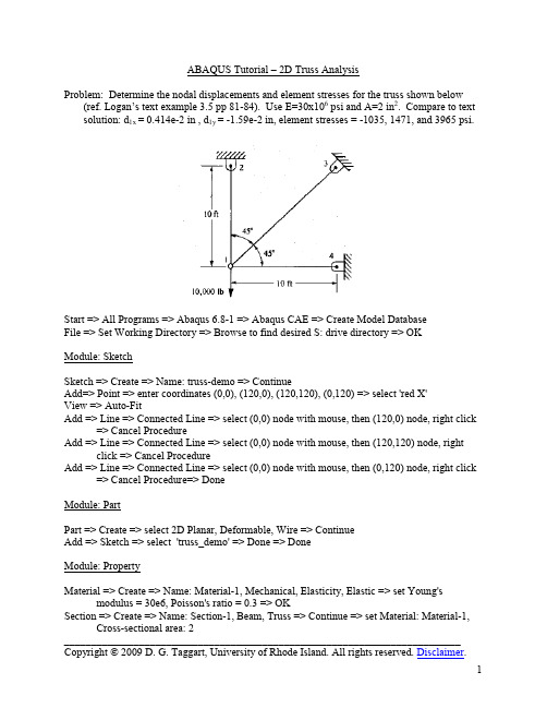
ABAQUS Tutorial – 2D Truss AnalysisProblem: Determine the nodal displacements and element stresses for the truss shown below (ref. Logan’s text example 3.5 pp 81-84). Use E=30x106 psi and A=2 in2. Compare to text solution: d1x = 0.414e-2 in , d1y = -1.59e-2 in, element stresses = -1035, 1471, and 3965 psi.Start => All Programs => Abaqus 6.8-1 => Abaqus CAE => Create Model DatabaseFile => Set Working Directory => Browse to find desired S: drive directory => OKModule: SketchSketch => Create => Name: truss-demo => ContinueAdd=> Point => enter coordinates (0,0), (120,0), (120,120), (0,120) => select 'red X'View => Auto-FitAdd => Line => Connected Line => select (0,0) node with mouse, then (120,0) node, right click => Cancel ProcedureAdd => Line => Connected Line => select (0,0) node with mouse, then (120,120) node, right click => Cancel ProcedureAdd => Line => Connected Line => select (0,0) node with mouse, then (0,120) node, right click => Cancel Procedure=> DoneModule: PartPart => Create => select 2D Planar, Deformable, Wire => ContinueAdd => Sketch => select 'truss_demo' => Done => DoneModule: PropertyMaterial => Create => Name: Material-1, Mechanical, Elasticity, Elastic => set Young's modulus = 30e6, Poisson's ratio = 0.3 => OKSection => Create => Name: Section-1, Beam, Truss => Continue => set Material: Material-1, Cross-sectional area: 2__________________________________________________________________________ Copyright © 2009 D. G. Taggart, University of Rhode Island. All rights reserved. Disclaimer.Assign Section => select all elements by dragging mouse => Done => Section-1 => OK => DoneModule: AssemblyInstance => Create => Part-1 => Independent (mesh on instance) => OKModule: StepStep => Create => Name: Step-1, Initial, Static, General => Continue => accept default settings => OKModule: LoadLoad => Create => Name: Step-1, Step: Step 1, Mechanical, Concentrated Force => Continue => select node at (0,0) => Done => set CF2: -10000 => OKBC => Create => Name: BC-1, Step: Step-1, Mechanical, Displacement/Rotation => Continue => select nodes at (120,0), (120,120) and (0,120) using SHIFT key to select multiplenodes => Done => set U1: 0 and U2: 0Module: MeshSeed => Edge by Number => select entire truss by dragging mouse => Done => Number of elements along edges: 1 => press Enter => DoneMesh => Element Type => select entire truss by dragging mouse => Done => Element Library: Standard, Geometric Order: Linear: Family: Truss => OK => DoneMesh => Instance => OK to mesh the part Instance: YesModule: JobJob => Create => Name: Job-1, Model: Model-1 => Continue => Job Type: Full analysis, Run Mode: Background, Submit Time: Immediately => OKJob => Submit => Job-1Job => Manager => Results (enters Module: Visualization)Plot = > Allow multiple plot statesPlot => Undeformed ShapePlot => Deformed ShapePlot => Contours => On Deformed ShapeResult => Options => unselect “Average element output at nodes”View => Graphics Options => Viewport Background = Solid=> Color => White (click on black tile to change background color)Options => Common => Labels => select ‘Show element labels’ and ‘Show node labels’, set label colors to black => OKCtrl-C => Copies graphics window to clipboard => Paste in MS Word, etc.Report => Field Output => Variable => Position: Unique Nodal => select U: Spatial Displacements => Apply => Unselect UReport => Field Output => Variable => Position: Centroid => select S: Stress Components => Click on ‘>’ and unselect all stresses except S11 => ApplyOpen file ‘abaqus.rpt’ and cut and paste desired results into MS WordFile => Save => enter desired file name (Abaqus will append .cae)File => ExitResults:Deformed Mesh:Tabulated Results (using cut and paste from abaqus.rpt)Nodal displacements:Node U.Magnitude U.U1 U.U2 Label @Loc 1 @Loc 1 @Loc 1 -----------------------------------------------------------------1 16.3899E-03 4.14214E-03 -15.8579E-032 2.07107E-33 2.07107E-33 0.3 2.92893E-33 -2.07107E-33 -2.07107E-334 7.92893E-33 0. -7.92893E-33 Minimum 2.07107E-33 -2.07107E-33 -15.8579E-03 At Node 2 3 1 Maximum 16.3899E-03 4.14214E-03 0.At Node 1 1 2 Total 16.3899E-03 4.14214E-03 -15.8579E-03 Element Stresses:Element S.S11Label @Loc 1---------------------------------1 -1.03553E+032 1.46447E+033 3.96447E+03Minimum -1.03553E+03At Element 1Maximum 3.96447E+03At Element 3Total 4.39340E+03。
Abaqus-详细教程
第二章 ABAQUS基础一个完整的ABAQUS分析过程,通常由三个明确的步骤组成:前处理、模拟计算和后处理。
这三个步骤的联系及生成的相关文件如下:前处理(输入文件。
通常的做法是使用ABAQUS/CAE模拟计算(模拟计算阶段用二进制文件中以便进行后处理。
完成一个求解过程所需的时间可以从几秒钟到几天不等,这取决于所分析问题的复杂程度和计算机的运算能力。
后处理(ABAQUS/CAE)一旦完成了模拟计算得到位移、应力或其它基本变量,就可以对计算结果进行分析评估,即后处理。
通常,后处理是使用ABAQUS/CAE或其它后处理软件中的可视化模块在图形环境下交互式地进行,读入核心二进制输出数据库文件后,可视化模块有多种方法显示结果,包括彩色等值线图,变形形状图和x-y平面曲线图等。
2.1 ABAQUS分析模型的组成ABAQUS模型通常由若干不同的部件组成,它们共同描述了所分析的物理问题和所得到的结果。
一个分析模型至少要具有如下的信息:几何形状、单元特性、材料数据、荷载和边界条件、分析类型和输出要求。
几何形状有限单元和节点定义了ABAQUS要模拟的物理结构的基本几何形状。
每一个单元都代表了结构的离散部分,许多单元依次相连就组成了结构,单元之间通过公共节点彼此相互连结,模型的几何形状由节点坐标和节点所属单元的联结所确定。
模型中所有的单元和节点的集成称为网格。
通常,网格只是实际结构几何形状的近似表达。
网格中单元类型、形状、位置和单元的数量都会影响模拟计算的结果。
网格的密度越高(在网格中单元数量越大),计算结果就越精确。
随着网格密度增加,分析结果会收敛到唯一解,但用于分析计算所需的时间也会增加。
通常,数值解是所模拟的物理问题的近似解答,近似的程度取决于模型的几何形状、材料特性、边界条件和载荷对物理问题的仿真程度。
单元特性ABAQUS拥有广泛的单元选择范围,其中许多单元的几何形状不能完全由它们的节点坐标来定义。
例如,复合材料壳的叠层或工字型截面梁的尺度划分就不能通过单元节点来定义。
abaqus傻瓜教程6

产品虚拟设计综合实验上机指导书(ABAQUS篇)南京理工大学2009年12月1 引言 (3)2 ABAQUS 软件 (3)2.1 ABAQUS分析步骤 (3)2.2 ABAQUS/CAE简介 (4)2.3 单位制 (5)3 上机实验1——平面问题应力集中分析 (6)3.1 问题描述 (6)3.2 目的和要求 (6)3.3 操作步骤 (6)3.4 上机报告要求 (16)4 上机实验2——工字梁的模态分析 (17)4.1 问题描述 (17)4.2 目的和要求 (17)4.3 操作步骤 (17)4.4 上机报告要求 (21)5 上机实验3——瞬态动力学分析 (22)5.1 问题描述 (22)5.2 目的和要求 (22)5.3 操作步骤 (22)5.4 上机报告要求 (30)1 引言本篇是《产品虚拟设计综合实验》的第二部分——基于ABAQUS的机械产品性能分析。
通过上机,掌握ABAQUS软件的使用方法,学会利用有限元法分析工程问题,为将来在设计和研究中利用该类大型通用CAD/CAE软件进行工程分析奠定初步基础。
本手册涉及ABAQUS软件的静态分析、模态分析和动态分析。
2 ABAQUS 软件ABAQUS是一套功能强大的基于有限元法的工程模拟软件,其解决问题的范围从相对简单的线性分析到最富有挑战性的非线性模拟问题。
ABAQUS具备十分丰富的、可模拟任意实际形状的单元库,并与之对应拥有各种类型的材料模型库,可以模拟大多数典型工程材料的性能。
作为通用的模拟分析工具,ABAQUS不仅能解决结构分析中的问题(应力/位移),还能模拟和研究其它各种领域中的问题,如热传导、质量扩散、电子元器件的热控制(热——电耦合分析)、声学分析、土壤力学分析(渗流——应力耦合分析)和压电介质力学分析等。
2.1 ABAQUS分析步骤有限元分析包括以下三个步骤:前处理、分析计算和后处理,这三个步骤在ABAQUS/CAE中的实现方法如下。
1)前处理(ABAQUS/CAE)在前处理阶段需要定义物理问题的模型,并生成一个ABAQUS输入文件。
Abaqus软件使用英文教程SI...

Abaqus软件使⽤英⽂教程SI...Abaqus Student EditionInstallation InstructionsBefore you begin:1.Make sure you have administrator privileges, as this is required for the Abaqus StudentEdition installation.2.Turn off all anti-virus software.3.If your PC has Windows User Access Control active, we recommend turning UAC down to itslowest settings.4.Only 64-bit Windows operating systems are allowed, not 32-bit Windows. If you areunsure, try the following: Start -> Run“cmd” and type “systeminfo” in the commandwindow. If the “System type” field says “X86-based PC, you have a 32-bit OS. If it says “X64-based PC”, you have a 64-bit OS.The Abaqus Student Edition installation consists of 3 basic sections.a)Abaqus HTML Documentation Installationb)Abaqus Product Installationc)Abaqus Installation VerificationDetailed steps for all sections are included below. The images shown below are from an installation of Abaqus 6.14-2 Student Edition on Windows 8. Other operating systems may look slightlydifferent.Step 1Download the Abaqus Student Edition executable file.Abaqus_6.14-2SE_win86_64, for 64-bit Windows, is 1.77 GB in size.Double-click the executable to begin the file extraction and installation process. Click Yes .Step 3Allow at least 5 minutes for the installation data to extract to your machine.When it is complete, the Abaqus Product Installer will launch automatically.Read and accept the terms of the license agreement to continue. Click Next .Read the information and Click Next to continue with the installation.If there are no previous Abaqus installations on your computer, you will be asked to provide an installation directory. Otherwise, the Abaqus 6.14 Student Edition will be installed in the same directory as any previous installations.Choose your installation directory and click Next .Choose the location for all your Abaqus job files and click Next .installation will begin.First, the Abaqus Student Edition HTML Documentation is installed. This process may take up to 30 minutes to complete.After the documentation installation completes the Abaqus Student Edition product installation will proceed without further input.Step 11Once the Abaqus product installation has completed, the product verification begins automatically.After verification completes, a results panel is displayed for your review.If any errors are displayed, click the verify.html link for additional information and troubleshooting.After clicking Next the final screen will appear, giving you the necessary information to launch the Abaqus Student Edition software. Clicking Done will finish the installation and exit the window.Execute the newly installed Student Edition product:On Windows 7 and earlier, from the shortcuts in the Start menu under Programs -> Abaqus 6.14 Student EditionOn Windows 8, from the icons in the Apps screen under section Abaqus 6.14 Student EditionKnown issue:On Windows 8, uninstall of Abaqus 6.14 Student Edition will uninstall the Abaqus product but not the documentation.o To uninstall Abaqus 6.14-2 Student Edition documentation:1.Ensure your account has Administrator privileges.2.From the Start screen, select Desktop./doc/741dedc0c67da26925c52cc58bd63186bdeb920b.html unch File Explorer (Folder icon in the lower left of the taskbar).4.From File Explorer in field at the top of the window, launch theuninstaller executable from the installation directory.For example:If your Abaqus installation directory was C:\SIMULIA it would be locatedat:C:\SIMULIA\Documentation\installation_info\v6.14\html_uninstaller\Uninstall Abaqus 6.14 Student Edition.exe5.Follow the prompts to perform the uninstallation.。
Lab10-AbaqusBucklingTutorial
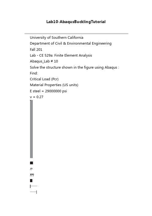
Lab10-AbaqusBucklingTutorialUniversity of Southern CaliforniaDepartment of Civil & Environmental Engineering Fall 201Lab - CE 529a: Finite Element AnalysisAbaqus_Lab # 10Solve the structure shown in the figure using Abaqus : Find:Critical Load (Pcr)Material Properties (US units)E steel = 29000000 psiν = 0.27P8 in60 inAnalysis Steps1. Start Abaqus New model database2. Double click on “Parts” node in the model tree3. In “Create Part” Select:2D PlanarDeformableWireApproximate Size : 2004. Draw the geometry of the Column5. Double click on “Materials” node in the model treeName the material and write a description Select: Mechanical Elasticity Elastic Define Young’s Modulus and Poisson’s R. Click “OK”6. Double click on “Profiles” node in the model treeName the Profile Select “Pipe” profile Click “Continue…”Enter the values for the profileClick “OK”7. Double click on “Sections” node in the model treeName the SectionSelect Category BeamSelect Type BeamClick “Continue…”Select Material SteelProfile name “Pipe-Column”Click “OK”8. Expand the “Parts” node in the model tree and expand the p art (Column) created, and double click on “SectionAssigment”Select the columnClick “Done” in the prompt areaSelect Section “Column”Click “OK”9. Select “Assign Beam Orientation” icon- Select the element and Click “Done” in the prompt area- Click “Enter”- Select “Ok” in the prompt area and then Click “Done” in the prompt area10. Expand the “Assembly” node in the model tree and then double click on “Instances”Select Parts : ColumnSelect “Independent”Click “OK”11. Select “Mesh” in Module combo boxIn the toolbox area click on the “Seed Part Instance” icon Approximate global size : 2Click “OK”Click “Done” in the prompt area12. In the toolbox area click on the “Assign Element Type” iconElement Library StandardFamily BeanGeometric Order LinearBeam type Cubic formulationClick “OK”Click “Done” in the prompt area13. In the toolbox area click on the “Mesh Part Instance” icon- Click “Yes” in the prompt area14. (Optional) In the menu bar select View Assembly Display Options…Select Mesh tab Check “Show node label”Check “Show element labels” Click “OK” Now You can see the nodes labelsNote: In the Tab “General” you can selectRender beam Profile and this showa Render of the sections.15. Double click on the “Steps” node in the model treeName StepSelect Linear perturbation BuckleClick “Continue…”Give a Step DescriptionNumber of eigenvalues requested ; 6Maximum number of iterations: 100Click “OK”16. Double click on the “BCs” node in the model treeName the BCSelect Step “Step-Buckling”Select Category MechanicalSelect Types for Selected Step Displacement/ Rot Click “Continue…”Select Node for the Pinned support and press “Done” in the prompt areaCheck the U1 and U2Set them to 017. In the toolbox area click on the “Create Boundary Condition” iconName the BCSelect Step “Step-Buckling”Select Category MechanicalSelect Types for Selected Step Displacement/ RotClick “Continue…”Select Node for the Roller support and press “Done” in the prompt areaCheck the U1 Set them to 018. In the toolbox area click on the “Create Load” iconName the LoadSelect Step “Step-Buckling”Select Category MechanicalSelect Mechanical Concentrated forceClick Continue…Select Node for the Load and press “Done” in the prompt areaSpecify CF1 = 0Specify CF2 = -1Click “OK”19. Double click on the “Jobs” node in the model treeName JobClick “Continue…”Give a DescriptionClick “OK20. Right click on the “Jobs” node in the model tree, and select “Submit”Check that there are no errors or warningsIf there errors, investigate the cause(s) and fixe themIf there warnings, investigate the cause(s)21. Right click on the Job - Buckling (Completed) and select Results22. In the toolbox area click on the “Plot Contours on Deformed Shape” iconAmplification value to obtain the critical loadL dLoadExample HW report:Critical Load : Pcr = 3633290 lbs。
- 1、下载文档前请自行甄别文档内容的完整性,平台不提供额外的编辑、内容补充、找答案等附加服务。
- 2、"仅部分预览"的文档,不可在线预览部分如存在完整性等问题,可反馈申请退款(可完整预览的文档不适用该条件!)。
- 3、如文档侵犯您的权益,请联系客服反馈,我们会尽快为您处理(人工客服工作时间:9:00-18:30)。
1
e. A general look of CAE is as follows:
Figure 1. General Look of CAE GUI f. To work through these steps you will work with individual modules in CAE. g. CAE modules: Unless like in ANSYS, you have different modules here. They are as follows: i. ii. iii. iv. v. vi. vii. viii. ix. Part – Create individual parts Property – Create and assign material properties. Assembly – Create and place all parts instances Step – Define all analysis steps and the results you want Interaction – Define any contact information Load- Define and place all loads and boundary conditions Mesh – Define your nodes and elements Job – Submit your job for analysis Visualization- View your results
other end of the rectangle (10, 2) and press enter. Click the mouse button 2 anywhere in the view port to finish using the rectangle tool. (If you are using a 2button mouse, press both mouse buttons simultaneously).If you made some mistakes in drawing you can click Delete to make changes. Click done in the prompt area after finishing drawing. Note: Save your model using File > Save/Save As. Save your work in regular intervals using the Save button in the main menu bar.
2. Little more on ABAQUS/CAE: Its better we know the general structure of
CAE before we start working with it. So, let us have some Knowledge transfer! a. ABAQUS CAE creates a binary file with a .cae file extension. When viewing your results it uses the .odb and .fil files b. CAE created an input file to run the analysis. c. You can import an input file to CAE to manipulate the model d. In CAE you make parts, and then assemble those parts into a model which is then analyzed.
3. Creating a model:
a. In the Context bar under Module, select Part if not loaded already. Click on “Create Part” in the toolbox area. Name the part Beam or something you like. Make sure you set Modeling Space to 2D Planar, Type to Deformable, and Base Feature to Shell (Shell for Area; Wire for Line; Point for Point). In the Approximate Size text field type 30 or any value that would be appropriate for your FE model size. Note that the approximate size will not affect your solution. Click Continue to exit the Create Part dialog box. b. Click Create Lines: Rectangle (4 Lines) in the toolbox to draw the cantilever beam. In the Prompt area type (0, 0) and press enter, give coordinates for the 2
1. பைடு நூலகம்aunching Abaqus/CAE
a. Log into Hammer using a SSH client b. Create a separate directory with „mkdir‟ command in your home directory for abaqus analysis. c. Change the directory to the new directory d. Type „abaqus cae’ to launch Abaqus/CAE e. When it starts click on Create Model Database. f. If you want to assign a name to your model, then go to main menu: Model > Manager. Click Rename, type 2D Cantilever Beam or something you like and Click Dismiss.
4. Creating a part
a. In the context bar under Module, select Property. You will see that a new set of tools appear in the toolbox area. Click on Create Material. Edit Material dialog box appears. Name the material (say, Steel) and click on Mechanical > Elasticity > Elastic. Leave Type as Isotropic and fill in the value of Young’s Modulus as 30e6 and Poisson’s ratio as 0.3. Click OK. b. Click on Create Section in the toolbox to define a section. Name the new section as you like (say, BeamSection), set Category to Solid and Type to Homogenous and click Continue. Accept the default selection of Steel for the Materials and Type 0.375 in the Plane Stress/Strain thickness. Click OK. c. Click on Assign Section in the toolbox. Click anywhere in the beam to select it (Note: If you have to select more than one thing, you can use the Shift key for multiple selections). Click Done in the prompt area to accept the selected geometry. The Edit Section Assignment Dialog Box appears containing a list of existing sections. Accept the default selection of BeamSection as the section and click OK. ABAQUS/CAE changes the color of the entire beam to aqua to indicate the region has a section assignment. When you assign a section to a region of a part, the region takes on the material properties associated with the section. d. Assembling the Model: Load the Assembly module from the Context bar. Click on Instance Part button from the toolbox, and Create Instance dialog box appears. Click on Independent (mesh on instance) and click OK. e. Defining Analysis Steps: In the Context bar under Module, select Step. Click on the Create Step button in the toolbox. Name the step (say, BeamLoad) and make sure you define a step of Static, General. Click Continue and accept all the default settings. Click OK. f. For the output we want stresses, strains, displacements, and forces/reaction. Set this in Field Output request option of the model tree.