Lethal response of the dengue vectors to the plant extracts from family Anacardiaceae简

合集下载

Screening mass responses to the chemical potential at finite temperature

†
−5 0.00
0.01 ma
0.02
0.03
(4) .
ˆ 2 /dµ Figure 1. d2 M ˆ2 S for the pseudoscalar meson versus ma at T < Tc (β = 5.26, triangles) and T > Tc (β = 5.34, circles). Extrapolation to ma = 0 is also shown.
−
Lx 2
10
L2 + x 4 Lx x ˆ− 2 .
5
0
−Lx
ˆ tanh M
In this work, we consider the ﬂavor non-singlet mesons in QCD with two ﬂavors. The hadron correlator is then given by H (n)H (0)† = = G Tr P (ˆ µu )n0 ΓP (ˆ µd )0n Γ
3. Numerical Simulations and Results The simulations have been performed at ﬁnite temperature T /Tc ∈∼ [0.9, 1.1] on a 16 × 82 × 4 lattice with standard Wilson gauge action and with two dynamical ﬂavors of staggered quarks. We use the R-algorithm, with quark masses ma = 0.0125, 0.017 and 0.025. We also use a cornertype wall source after Coulomb gauge ﬁxing in each (y, z, t)-hyperplane. The ﬁrst derivative of the pseudoscalar meson correlator with respect to the isoscalar chemical potential is identically zero. For the isovector chemical potential, our simulation values for the ﬁrst derivative are very small in both phases. 3.1. Response of the pseudoscalar meson to the isoscalar chemical potential In the low temperature phase, the dependence of the mass on µ ˆ S is small. This behavior is to be expected, since, below the critical temperature and in the vicinity of zero µ ˆS , the pseudoscalar meson is still a Goldstone boson. In fact, the chiral extrapolation of the isoscalar response is

Phase Preserving Denoising of Images

Phase Preserving Denoising of ImagesPeter KovesiDepartment of Computer ScienceThe University of Western AustraliaNedlands,W.A.6907pk@.auAbstractIn recent years wavelet shrinkage denoising has become the method of choice for the denoising of images.However, despite much research a number of questions remain.-Which of the many wavelets that exist should one use?-How should the threshold be set?and-How are features in the image affected by the thresholding operation?This paper explores these issues and argues for the use of non-orthogonal,complex valued,log-Gabor wavelets, rather than the more usual orthogonal or bi-orthogonal wavelets.Thresholding of wavelet responses in the complex domain allows one to ensure that perceptually important phase information in the image is not corrupted.It is also shown how appropriate threshold values can be determined automatically from the statistics of the wavelet responses to the image.1.IntroductionDenoising of images is typically done with the following process:The image is transformed into some domain where the noise component is more easily identiﬁed,a threshold-ing operation is then applied to remove the noise,andﬁnally the transformation is inverted to reconstruct a(hopefully) noise-free image.The wavelet transform has proved to be very successful in making signal and noise components of the signal dis-tinct.As wavelets have compact support the wavelet co-efﬁcients resulting from the signal are localised,whereas the coefﬁcients resulting from noise in the signal are dis-tributed.Thus the energy from the signal is directed into a limited number of coefﬁcients which‘stand out’from the noise.Wavelet shrinkage denoising then consists of identi-fying the magnitude of wavelet coefﬁcients one can expect from the noise(the threshold),and then shrinking the mag-nitudes of all the coefﬁcients by this amount.What remains of the coefﬁcients should be valid signal data,and the trans-form can then be inverted to reconstruct an estimate of the signal[4,3,1].Wavelet denoising has concentrated on the use of or-thogonal or bi-orthogonal wavelets because of their recon-structive qualities.However,no particular wavelet has been identiﬁed as being the‘best’for denoising.It is generally agreed that wavelets having a linear-phase,or near linear-phase,response are desirable,and this has led to the use of the‘symlet’series of wavelets and bi-orthogonal wavelets.A problem with wavelet shrinkage denoising is that the discrete wavelet transform is not translation invariant.If the signal is displaced by one data point the wavelet coef-ﬁcients do not simply move by the same amount.They are completely different because there is no redundancy in the wavelet representation.Thus,the shape of the reconstructed signal after wavelet shrinkage and transform inversion will depend on the translation of the signal-clearly this is not very satisfactory.To overcome this translation invariant de-noising has been devised[1].This involves averaging the wavelet shrinkage denoising result over all possible transla-tions of the signal.This produces very pleasing results and overcomes pseudo-Gibbs phenomena that is often seen in the basic wavelet shrinkage denoising scheme.The criteria for quality of the reconstructed noise-free image has generally been the RMS error-though Donoho suggests a side condition that the reconstructed(denoised) signal should be,with high probability,as least as smooth as the original(noise free)signal.While the use of the RMS error in reconstructing1D sig-nals may be reasonable,the use of the RMS measure for im-age comparison has been criticised[2,10].Almost without exception images exist solely for the beneﬁt of the human visual system.Therefore any metric that is used for evaluat-ing the quality of image reconstruction must have relevance to our visual perception system.The RMS error certainly does not necessarily give a good guide to the perceptual quality of an image reconstruction.For example,displac-ing an image a small amount,or offsetting grey levels bya small amount,will have negligible perceptual effect,but will induce a large RMS error.As yet no metric that matches human visual perception has been devised.However,one quantity that appears to be very important in the human perception of images is phase. The classic demonstration of the importance of phase was devised by Oppenheim and Lim[9].They took the Fourier transforms of two images and used the phase information from one image and the magnitude information of the other to construct a new,synthetic Fourier transform which was then back-transformed to produce a new image.The fea-tures seen in such an image,while somewhat scrambled, clearly correspond to those in the image from which the phase data was obtained.Little evidence,if any,from the other image can be perceived.A demonstration of this isrepeated here in Figure1.+=Figure1.When phase information from oneimage is combined with magnitude informa-tion of another it is phase information thatprevails.While phase is not the only quantity important to our perception of images it would seem that an important con-straint that should be satisﬁed by any image enhancement process,such as denoising,is that it should not corrupt the phase information in an image2.Phase Preserving DenoisingTo be able to preserve the phase data in an image we have toﬁrst extract the local phase and amplitude informa-tion at each point in the image.This can be done by apply-ing(a discrete implementation of)the continuous wavelet transform and using wavelets that are in symmetric/anti-symmetric pairs.Here we follow the approach of Mor-let,that is,using wavelets based on complex valued Ga-bor functions-sine and cosine waves,each modulated by a Gaussian[8].Using twoﬁlters in quadrature enables one to calculate the amplitude and phase of the signal for a partic-ular scale/frequency at a given spatial location.However,rather than using Gaborﬁlters we prefer to use log Gabor functions as suggested by Field[5];these areﬁl-ters having a Gaussian transfer function when viewed on the logarithmic frequency scale.Log Gaborﬁlters allow arbi-trarily large bandwidthﬁlters to be constructed while still maintaining a zero DC component in the even-symmetric ﬁlter.A zero DC value cannot be maintained in Gabor func-tions for bandwidths over1octave.It is of interest to note that the spatial extent of log Gaborﬁlters appears to be min-imized when they are constructed with a bandwidth of ap-proximately two octaves[7,6].This would appear to be op-timal for denoising as this will minimise the spatial spread of wavelet response to signal features,and hence concen-trate as much signal energy as possible into a limited num-berofcoefﬁcients.Figure2.Even and odd log Gabor wavelets,each having a bandwidth of two octaves.Analysis of a signal is done by convolving the signal with each of the quadrature pairs of wavelets.If we let denote the signal and and denote the even-symmetric and odd-symmetric wavelets at a scale we can think of the responses of each quadrature pair ofﬁlters as forming a re-sponse vector,The values and can be thought of as real and imaginary parts of complex valued frequency component. The amplitude of the transform at a given wavelet scale is given byodd symmetric filter outputeven symmetric filter outputfrequencyphaseFigure 3.An array of ﬁlter response vectors at a point in a signal can be represented as a series of vectors radiating out from the fre-quency axis.The amplitude speciﬁes the length of each vector and the phase speciﬁes its angle.Note that wavelet ﬁlters are scaled geometrically,hence their centre frequencies vary accordingly.shrunken response vectoreven filter responseretained for reconstructionnoise thresholdfilter response vector(imaginary axis)odd filter response even filter response (real axis)Figure 4.View along the frequency axis il-lustrating the shrinkage of complex-valued wavelet response vectors.the threshold because the shrinkage process is constrained to operate only on the real axis.Note also that applying shrinkage only along the real axis will corrupt phase infor-mation as the imaginary component will be ignored in de-ciding how much a wavelet component should be shrunk.It is worth noting that the averaging process in translation-invariant denoising may achieve a similar result to the pro-posed phase preserving algorithm.Having shrunk the complex-valued wavelet response vectors an estimate of the signal can then be reconstructed by summing the remaining even-symmetric ﬁlter responses over all scales and orientations.However,there are some issues in the reconstruction of the denoised image from the shrunk response plex valued log Gabor ﬁlters do not form an orthogonal basis set.This means that the sig-nal can only be reconstructed over the range of frequencies covered by the ﬁlters,and that the signal can only be recon-structed up to a scale factor.Thus to achieve satisfactoryreconstruction the design of the wavelet ﬁlter bank must be such that the transfer functions of all the ﬁlters overlap suf-ﬁciently so that their sum results in an even coverage of the spectrum.In the 2D frequency plane the ﬁlter transfer func-tions appear as 2D log Gaussians.These can be arranged in a ‘rosette’to ensure uniform coverage of the spectrum.Un-der this arrangement it is difﬁcult to have ﬁlters that cover the very low frequencies in the image.However,perceptu-ally this does not appear to be very important.Similarly,the lack of an absolute scale in the reconstructed grey levels is not important perceptually.3.Determining the ThresholdThe most crucial parameter in the denoising process is the threshold.While many techniques have been devel-oped [4,3]none have proved very satisfactory.Here we develop an automatic thresholding scheme.First we must look at the expected response of the ﬁlters to a pure noise signal.If the signal is purely Gaussian white noise the positions of the resulting response vectors from a wavelet quadrature pair of ﬁlters at some scale will form a 2D Gaussian distribution in the complex plane.What we are interested in is the distribution of the magnitude of the response vectors.This will be a Rayleigh distributionwhere is the variance of the 2D Gaussian distribution describing the position of the ﬁlter response vectors.The mean of the Rayleigh distribution is given byand the variance is0.511.522.533.540.10.20.30.40.50.60.70.8Figure 5.Rayleigh distribution with a mean of one.response,but the regions where it will be responding to fea-tures will be small due to the small spatial extent of the ﬁlter.Thus the smallest scale wavelet quadrature pair will spend most of their time only responding to noise.Thus,the distribution of the amplitude response from the smallest scale ﬁlter pair across the whole image will be pri-marily the noise distribution,that is,a Rayleigh distribution with some contamination as a result of the response of the ﬁlters to feature points in the image.We can obtain a robust estimate of the mean of the am-plitude response of the smallest scale ﬁlter via the median response.The median of a Rayleigh distribution is the value such thatNoting that the mean of the Rayleigh distribution iswe obtain the expected value of the amplitude response of the smallest scale ﬁlter (the estimate of the mean)where is the index of the smallest scale ﬁlter.Giventhatwe can then estimate and for thenoise response for the smallest scale ﬁlter pair,and hencethe shrinkage threshold.We can estimate the appropriate shrinkage thresholds to use at the other ﬁlter scales if we make the following ob-servation:If it is assumed that the noise spectrum is uni-form then the wavelets will gather energy from the noise as a function of their bandwidth which,in turn,is a function of their centre frequency.For 1D signals the amplitude re-sponse will be proportional to the square root of the ﬁltercentre frequency.In 2D images the amplitude response will be directly proportional to the ﬁlter centre frequency.wavelet amplitude responseW2W3A2Aωnoise power spectrumwavelet 3ωwavelet 2wavelet 1frequency bandW1log Figure 6.If the noise spectrum is uniform the response of a wavelet to the noise will be a function of its bandwidth.Thus having obtained an estimate of the noise amplitude distribution for the smallest scale ﬁlter pair we can simply scale this appropriately to form estimates of the noise am-plitude distributions at all the other scales.This approach proves to be very successful in allowing shrinkage thresh-olds to be set automatically from the statistics of the small-est scale ﬁlter response over the whole image.4.ResultsFigure 7shows a synthetic test image with grey values ranging between 0and 255.Gaussian white noise with a standard deviation of 80grey levels was added to the im-age.The result of applying the phase preserving denoising algorithm to the image (using a value of 2to set the thresh-old)is shown along with the result obtained by applying a standard discrete wavelet denoising scheme (the MATLAB wdencmp function using the ‘symlet8’wavelet and a man-ually derived threshold of 60).Figure 8shows the 1D sections at row 150(out of 256)on each of the four images shown in Figure 7.Note the vertical scale for the plot of the phase preserved denoised image does not match that for the original image.The re-construction from the complex-valued log Gabor wavelets cannot cover the very low,and zero frequency,components of the signal.Also the signal can only be recovered up to a scale factor.Despite this the shape of the reconstructed signal is very good.A major part of the success of the seemingly astonishing reconstruction is due to the fact that the denoising process is taking place in 2D.The reconstruc-tion of row 150in the image makes use of information from above and below that row.Such a result would not be pos-sible working solely in 1D.Figure 9shows the phase preserving denoising process applied to a poor quality surveillance image of a hold-up.It should be noted that video images consist of two interlaced images.If there is any motion (there was a small amount in this image)the interlacing will result in ‘tooth comb’edgesTestimage Noisy testimageDenoised using symlet8waveletDenoised with phase pre-servedFigure7.Denoising of a test imagearound objects.To overcome this the individual images thatmake up the video frame can be obtained by extracting justthe even,or just the odd,numbered scan lines from the im-age prior to denoising.5.ConclusionWe have presented a new denoising algorithm,basedon the decomposition of a signal using complex-valuedwavelets.This algorithm preserves the perceptually im-portant phase information in the signal.In conjunctionwith this a method has been devised to automatically de-termine the appropriate wavelet shrinkage thresholds fromthe statistics of the amplitude response of the smallest scaleﬁlter pair over the image.The automatic determination ofthresholds overcomes a problem that has plagued waveletdenoising schemes in the past.The RMS measure is not always the most appropriatemetric to use in the development of image processing algo-rithms.Indeed it could be argued that more time should bespent optimising the choice of the optimisation criteria ingeneral.For images it would appear that the preservation ofphase data is important,though of course,other factors mustalso be important.The denoising algorithm presented hereFigure8.Section along row150in the test im-agedoes not seek to do any optimisation,it has merely beenconstructed so as to satisfy the constraint that phase shouldnot be corrupted.Given that it satisﬁes this constraint,itshould be possible to develop it further so that it does in-corporate some optimisation,say,the minimisation of thedistortion of the signal’s amplitude spectrum.What shouldalso be investigated is the possible relationship between thisphase preserving algorithm and translation invariant denois-ing.References[1]R.R.Coifman and D.Donoho.Time-invariant waveletdenoising.In A.Antoniadis and G.Oppenheim,edi-tors,Wavelets and Statistics,volume103of Lecture Notesin Statistics,pages125–150,New York,1995.Springer-Verlag.[2]S.Daly.The visible diferences predictor:An algorithm forthe assessment of imageﬁdelity.In A.Watson,editor,Dig-ital Images and Human Vision,pages179–206.MIT Press,1993.[3] D.L.Donoho.De-noising by soft-thresholding.IEEETransactions on Information Theory,41(3):613–627,1995.[4] D.L.Donoho and I.M.Johnstone.Ideal spatial adaptationby wavelet shrinkage.Biometrika,81(3):425–455,1994.[5] D.J.Field.Relations between the statistics of natural imagesand the response properties of cortical cells.Journal of TheOptical Society of America A,4(12):2379–2394,December1987.[6]P.D.Kovesi.Image features from phase congruency.Videre:Journal of Computer Vision Research,to appear./e-journals/Videre/.[7]P.D.Kovesi.Invariant Measures of Image Features FromPhase Information.PhD thesis,The University of WesternAustralia,May1996.Original surveillance imageGrey scale enhanced surveil-lance imageImage obtained from just the odd numbered scan lines Denoised with phase pre-servedFigure 9.Denoising of a surveillance image[8]J.Morlet,G.Arens,E.Fourgeau,and D.Giard.Wavepropagation and sampling theory -Part II:Sampling theory and complex waves.Geophysics ,47(2):222–236,February 1982.[9] A.V .Oppenheim and J.S.Lim.The importance of phasein signals.In Proceedings of The IEEE 69,pages 529–541,1981.[10] D.Wilson,A.Baddeley,and R.Owens.A new metricfor grey-scale image comparison.International Journal of Computer Vision ,24(1):5–17,1997.。

登革热

物能携带登革热病毒）是本病主要传染源和宿主 • 2.传播途径：蚊媒传播，登革热在我国的主要传播媒介为埃及伊蚊和白纹伊蚊 • 3.人群易感性及免疫性：人类对登革热不分种族、年龄、
性别普遍易感，但感染后仅有部分人发病。人初次感染登
革病毒后对同型病毒有较巩固的免疫力，可持续数年，但对异型登革病毒免疫力只能维持很短时间 • 4.潜伏期：3-14天
• 2.3 伴面部、颈部、胸部潮红，结膜出血；
• 2.4 浅表淋巴结肿大； • 2.5 皮疹：于病程3～7天出现为多样性皮疹（麻疹样、猩红热样）、皮下出血点等。皮疹分布于四肢、躯干或头面部，多有痒感，不脱屑。持续3～5天；
• 2.6 少数患者可表现为脑炎样脑病症状和体征；
• 2.7 有出血倾向（束臂试验阳性），一般在病程5～8天出
(various species)
Human African trypanosomiasis, onchocerciasis
Vector-borne diseases
Key facts • Vector-borne diseases account for more than 17% of all infectious diseases, causing more than 1 million deaths annually. • More than 2.5 billion people in over 100 countries are at risk of contracting dengue alone. • Malaria causes more than 600 000 deaths every year globally, most of them children under 5 years of age. • Other diseases such as Chagas disease, leishmaniasis and schistosomiasis affect hundreds of millions of people worldwide. • Many of these diseases are preventable through informed protective measures.

《神经网络与深度学习综述DeepLearning15May2014

Draft:Deep Learning in Neural Networks:An OverviewTechnical Report IDSIA-03-14/arXiv:1404.7828(v1.5)[cs.NE]J¨u rgen SchmidhuberThe Swiss AI Lab IDSIAIstituto Dalle Molle di Studi sull’Intelligenza ArtiﬁcialeUniversity of Lugano&SUPSIGalleria2,6928Manno-LuganoSwitzerland15May2014AbstractIn recent years,deep artiﬁcial neural networks(including recurrent ones)have won numerous con-tests in pattern recognition and machine learning.This historical survey compactly summarises relevantwork,much of it from the previous millennium.Shallow and deep learners are distinguished by thedepth of their credit assignment paths,which are chains of possibly learnable,causal links between ac-tions and effects.I review deep supervised learning(also recapitulating the history of backpropagation),unsupervised learning,reinforcement learning&evolutionary computation,and indirect search for shortprograms encoding deep and large networks.PDF of earlier draft(v1):http://www.idsia.ch/∼juergen/DeepLearning30April2014.pdfLATEX source:http://www.idsia.ch/∼juergen/DeepLearning30April2014.texComplete BIBTEXﬁle:http://www.idsia.ch/∼juergen/bib.bibPrefaceThis is the draft of an invited Deep Learning(DL)overview.One of its goals is to assign credit to those who contributed to the present state of the art.I acknowledge the limitations of attempting to achieve this goal.The DL research community itself may be viewed as a continually evolving,deep network of scientists who have inﬂuenced each other in complex ways.Starting from recent DL results,I tried to trace back the origins of relevant ideas through the past half century and beyond,sometimes using“local search”to follow citations of citations backwards in time.Since not all DL publications properly acknowledge earlier relevant work,additional global search strategies were employed,aided by consulting numerous neural network experts.As a result,the present draft mostly consists of references(about800entries so far).Nevertheless,through an expert selection bias I may have missed important work.A related bias was surely introduced by my special familiarity with the work of my own DL research group in the past quarter-century.For these reasons,the present draft should be viewed as merely a snapshot of an ongoing credit assignment process.To help improve it,please do not hesitate to send corrections and suggestions to juergen@idsia.ch.Contents1Introduction to Deep Learning(DL)in Neural Networks(NNs)3 2Event-Oriented Notation for Activation Spreading in FNNs/RNNs3 3Depth of Credit Assignment Paths(CAPs)and of Problems4 4Recurring Themes of Deep Learning54.1Dynamic Programming(DP)for DL (5)4.2Unsupervised Learning(UL)Facilitating Supervised Learning(SL)and RL (6)4.3Occam’s Razor:Compression and Minimum Description Length(MDL) (6)4.4Learning Hierarchical Representations Through Deep SL,UL,RL (6)4.5Fast Graphics Processing Units(GPUs)for DL in NNs (6)5Supervised NNs,Some Helped by Unsupervised NNs75.11940s and Earlier (7)5.2Around1960:More Neurobiological Inspiration for DL (7)5.31965:Deep Networks Based on the Group Method of Data Handling(GMDH) (8)5.41979:Convolution+Weight Replication+Winner-Take-All(WTA) (8)5.51960-1981and Beyond:Development of Backpropagation(BP)for NNs (8)5.5.1BP for Weight-Sharing Feedforward NNs(FNNs)and Recurrent NNs(RNNs)..95.6Late1980s-2000:Numerous Improvements of NNs (9)5.6.1Ideas for Dealing with Long Time Lags and Deep CAPs (10)5.6.2Better BP Through Advanced Gradient Descent (10)5.6.3Discovering Low-Complexity,Problem-Solving NNs (11)5.6.4Potential Beneﬁts of UL for SL (11)5.71987:UL Through Autoencoder(AE)Hierarchies (12)5.81989:BP for Convolutional NNs(CNNs) (13)5.91991:Fundamental Deep Learning Problem of Gradient Descent (13)5.101991:UL-Based History Compression Through a Deep Hierarchy of RNNs (14)5.111992:Max-Pooling(MP):Towards MPCNNs (14)5.121994:Contest-Winning Not So Deep NNs (15)5.131995:Supervised Recurrent Very Deep Learner(LSTM RNN) (15)5.142003:More Contest-Winning/Record-Setting,Often Not So Deep NNs (16)5.152006/7:Deep Belief Networks(DBNs)&AE Stacks Fine-Tuned by BP (17)5.162006/7:Improved CNNs/GPU-CNNs/BP-Trained MPCNNs (17)5.172009:First Ofﬁcial Competitions Won by RNNs,and with MPCNNs (18)5.182010:Plain Backprop(+Distortions)on GPU Yields Excellent Results (18)5.192011:MPCNNs on GPU Achieve Superhuman Vision Performance (18)5.202011:Hessian-Free Optimization for RNNs (19)5.212012:First Contests Won on ImageNet&Object Detection&Segmentation (19)5.222013-:More Contests and Benchmark Records (20)5.22.1Currently Successful Supervised Techniques:LSTM RNNs/GPU-MPCNNs (21)5.23Recent Tricks for Improving SL Deep NNs(Compare Sec.5.6.2,5.6.3) (21)5.24Consequences for Neuroscience (22)5.25DL with Spiking Neurons? (22)6DL in FNNs and RNNs for Reinforcement Learning(RL)236.1RL Through NN World Models Yields RNNs With Deep CAPs (23)6.2Deep FNNs for Traditional RL and Markov Decision Processes(MDPs) (24)6.3Deep RL RNNs for Partially Observable MDPs(POMDPs) (24)6.4RL Facilitated by Deep UL in FNNs and RNNs (25)6.5Deep Hierarchical RL(HRL)and Subgoal Learning with FNNs and RNNs (25)6.6Deep RL by Direct NN Search/Policy Gradients/Evolution (25)6.7Deep RL by Indirect Policy Search/Compressed NN Search (26)6.8Universal RL (27)7Conclusion271Introduction to Deep Learning(DL)in Neural Networks(NNs) Which modiﬁable components of a learning system are responsible for its success or failure?What changes to them improve performance?This has been called the fundamental credit assignment problem(Minsky, 1963).There are general credit assignment methods for universal problem solvers that are time-optimal in various theoretical senses(Sec.6.8).The present survey,however,will focus on the narrower,but now commercially important,subﬁeld of Deep Learning(DL)in Artiﬁcial Neural Networks(NNs).We are interested in accurate credit assignment across possibly many,often nonlinear,computational stages of NNs.Shallow NN-like models have been around for many decades if not centuries(Sec.5.1).Models with several successive nonlinear layers of neurons date back at least to the1960s(Sec.5.3)and1970s(Sec.5.5). An efﬁcient gradient descent method for teacher-based Supervised Learning(SL)in discrete,differentiable networks of arbitrary depth called backpropagation(BP)was developed in the1960s and1970s,and ap-plied to NNs in1981(Sec.5.5).BP-based training of deep NNs with many layers,however,had been found to be difﬁcult in practice by the late1980s(Sec.5.6),and had become an explicit research subject by the early1990s(Sec.5.9).DL became practically feasible to some extent through the help of Unsupervised Learning(UL)(e.g.,Sec.5.10,5.15).The1990s and2000s also saw many improvements of purely super-vised DL(Sec.5).In the new millennium,deep NNs haveﬁnally attracted wide-spread attention,mainly by outperforming alternative machine learning methods such as kernel machines(Vapnik,1995;Sch¨o lkopf et al.,1998)in numerous important applications.In fact,supervised deep NNs have won numerous of-ﬁcial international pattern recognition competitions(e.g.,Sec.5.17,5.19,5.21,5.22),achieving theﬁrst superhuman visual pattern recognition results in limited domains(Sec.5.19).Deep NNs also have become relevant for the more generalﬁeld of Reinforcement Learning(RL)where there is no supervising teacher (Sec.6).Both feedforward(acyclic)NNs(FNNs)and recurrent(cyclic)NNs(RNNs)have won contests(Sec.5.12,5.14,5.17,5.19,5.21,5.22).In a sense,RNNs are the deepest of all NNs(Sec.3)—they are general computers more powerful than FNNs,and can in principle create and process memories of ar-bitrary sequences of input patterns(e.g.,Siegelmann and Sontag,1991;Schmidhuber,1990a).Unlike traditional methods for automatic sequential program synthesis(e.g.,Waldinger and Lee,1969;Balzer, 1985;Soloway,1986;Deville and Lau,1994),RNNs can learn programs that mix sequential and parallel information processing in a natural and efﬁcient way,exploiting the massive parallelism viewed as crucial for sustaining the rapid decline of computation cost observed over the past75years.The rest of this paper is structured as follows.Sec.2introduces a compact,event-oriented notation that is simple yet general enough to accommodate both FNNs and RNNs.Sec.3introduces the concept of Credit Assignment Paths(CAPs)to measure whether learning in a given NN application is of the deep or shallow type.Sec.4lists recurring themes of DL in SL,UL,and RL.Sec.5focuses on SL and UL,and on how UL can facilitate SL,although pure SL has become dominant in recent competitions(Sec.5.17-5.22). Sec.5is arranged in a historical timeline format with subsections on important inspirations and technical contributions.Sec.6on deep RL discusses traditional Dynamic Programming(DP)-based RL combined with gradient-based search techniques for SL or UL in deep NNs,as well as general methods for direct and indirect search in the weight space of deep FNNs and RNNs,including successful policy gradient and evolutionary methods.2Event-Oriented Notation for Activation Spreading in FNNs/RNNs Throughout this paper,let i,j,k,t,p,q,r denote positive integer variables assuming ranges implicit in the given contexts.Let n,m,T denote positive integer constants.An NN’s topology may change over time(e.g.,Fahlman,1991;Ring,1991;Weng et al.,1992;Fritzke, 1994).At any given moment,it can be described as aﬁnite subset of units(or nodes or neurons)N= {u1,u2,...,}and aﬁnite set H⊆N×N of directed edges or connections between nodes.FNNs are acyclic graphs,RNNs cyclic.Theﬁrst(input)layer is the set of input units,a subset of N.In FNNs,the k-th layer(k>1)is the set of all nodes u∈N such that there is an edge path of length k−1(but no longer path)between some input unit and u.There may be shortcut connections between distant layers.The NN’s behavior or program is determined by a set of real-valued,possibly modiﬁable,parameters or weights w i(i=1,...,n).We now focus on a singleﬁnite episode or epoch of information processing and activation spreading,without learning through weight changes.The following slightly unconventional notation is designed to compactly describe what is happening during the runtime of the system.During an episode,there is a partially causal sequence x t(t=1,...,T)of real values that I call events.Each x t is either an input set by the environment,or the activation of a unit that may directly depend on other x k(k<t)through a current NN topology-dependent set in t of indices k representing incoming causal connections or links.Let the function v encode topology information and map such event index pairs(k,t)to weight indices.For example,in the non-input case we may have x t=f t(net t)with real-valued net t= k∈in t x k w v(k,t)(additive case)or net t= k∈in t x k w v(k,t)(multiplicative case), where f t is a typically nonlinear real-valued activation function such as tanh.In many recent competition-winning NNs(Sec.5.19,5.21,5.22)there also are events of the type x t=max k∈int (x k);some networktypes may also use complex polynomial activation functions(Sec.5.3).x t may directly affect certain x k(k>t)through outgoing connections or links represented through a current set out t of indices k with t∈in k.Some non-input events are called output events.Note that many of the x t may refer to different,time-varying activations of the same unit in sequence-processing RNNs(e.g.,Williams,1989,“unfolding in time”),or also in FNNs sequentially exposed to time-varying input patterns of a large training set encoded as input events.During an episode,the same weight may get reused over and over again in topology-dependent ways,e.g.,in RNNs,or in convolutional NNs(Sec.5.4,5.8).I call this weight sharing across space and/or time.Weight sharing may greatly reduce the NN’s descriptive complexity,which is the number of bits of information required to describe the NN (Sec.4.3).In Supervised Learning(SL),certain NN output events x t may be associated with teacher-given,real-valued labels or targets d t yielding errors e t,e.g.,e t=1/2(x t−d t)2.A typical goal of supervised NN training is toﬁnd weights that yield episodes with small total error E,the sum of all such e t.The hope is that the NN will generalize well in later episodes,causing only small errors on previously unseen sequences of input events.Many alternative error functions for SL and UL are possible.SL assumes that input events are independent of earlier output events(which may affect the environ-ment through actions causing subsequent perceptions).This assumption does not hold in the broaderﬁelds of Sequential Decision Making and Reinforcement Learning(RL)(Kaelbling et al.,1996;Sutton and Barto, 1998;Hutter,2005)(Sec.6).In RL,some of the input events may encode real-valued reward signals given by the environment,and a typical goal is toﬁnd weights that yield episodes with a high sum of reward signals,through sequences of appropriate output actions.Sec.5.5will use the notation above to compactly describe a central algorithm of DL,namely,back-propagation(BP)for supervised weight-sharing FNNs and RNNs.(FNNs may be viewed as RNNs with certainﬁxed zero weights.)Sec.6will address the more general RL case.3Depth of Credit Assignment Paths(CAPs)and of ProblemsTo measure whether credit assignment in a given NN application is of the deep or shallow type,I introduce the concept of Credit Assignment Paths or CAPs,which are chains of possibly causal links between events.Let usﬁrst focus on SL.Consider two events x p and x q(1≤p<q≤T).Depending on the appli-cation,they may have a Potential Direct Causal Connection(PDCC)expressed by the Boolean predicate pdcc(p,q),which is true if and only if p∈in q.Then the2-element list(p,q)is deﬁned to be a CAP from p to q(a minimal one).A learning algorithm may be allowed to change w v(p,q)to improve performance in future episodes.More general,possibly indirect,Potential Causal Connections(PCC)are expressed by the recursively deﬁned Boolean predicate pcc(p,q),which in the SL case is true only if pdcc(p,q),or if pcc(p,k)for some k and pdcc(k,q).In the latter case,appending q to any CAP from p to k yields a CAP from p to q(this is a recursive deﬁnition,too).The set of such CAPs may be large but isﬁnite.Note that the same weight may affect many different PDCCs between successive events listed by a given CAP,e.g.,in the case of RNNs, or weight-sharing FNNs.Suppose a CAP has the form(...,k,t,...,q),where k and t(possibly t=q)are theﬁrst successive elements with modiﬁable w v(k,t).Then the length of the sufﬁx list(t,...,q)is called the CAP’s depth (which is0if there are no modiﬁable links at all).This depth limits how far backwards credit assignment can move down the causal chain toﬁnd a modiﬁable weight.1Suppose an episode and its event sequence x1,...,x T satisfy a computable criterion used to decide whether a given problem has been solved(e.g.,total error E below some threshold).Then the set of used weights is called a solution to the problem,and the depth of the deepest CAP within the sequence is called the solution’s depth.There may be other solutions(yielding different event sequences)with different depths.Given someﬁxed NN topology,the smallest depth of any solution is called the problem’s depth.Sometimes we also speak of the depth of an architecture:SL FNNs withﬁxed topology imply a problem-independent maximal problem depth bounded by the number of non-input layers.Certain SL RNNs withﬁxed weights for all connections except those to output units(Jaeger,2001;Maass et al.,2002; Jaeger,2004;Schrauwen et al.,2007)have a maximal problem depth of1,because only theﬁnal links in the corresponding CAPs are modiﬁable.In general,however,RNNs may learn to solve problems of potentially unlimited depth.Note that the deﬁnitions above are solely based on the depths of causal chains,and agnostic of the temporal distance between events.For example,shallow FNNs perceiving large“time windows”of in-put events may correctly classify long input sequences through appropriate output events,and thus solve shallow problems involving long time lags between relevant events.At which problem depth does Shallow Learning end,and Deep Learning begin?Discussions with DL experts have not yet yielded a conclusive response to this question.Instead of committing myself to a precise answer,let me just deﬁne for the purposes of this overview:problems of depth>10require Very Deep Learning.The difﬁculty of a problem may have little to do with its depth.Some NNs can quickly learn to solve certain deep problems,e.g.,through random weight guessing(Sec.5.9)or other types of direct search (Sec.6.6)or indirect search(Sec.6.7)in weight space,or through training an NNﬁrst on shallow problems whose solutions may then generalize to deep problems,or through collapsing sequences of(non)linear operations into a single(non)linear operation—but see an analysis of non-trivial aspects of deep linear networks(Baldi and Hornik,1994,Section B).In general,however,ﬁnding an NN that precisely models a given training set is an NP-complete problem(Judd,1990;Blum and Rivest,1992),also in the case of deep NNs(S´ıma,1994;de Souto et al.,1999;Windisch,2005);compare a survey of negative results(S´ıma, 2002,Section1).Above we have focused on SL.In the more general case of RL in unknown environments,pcc(p,q) is also true if x p is an output event and x q any later input event—any action may affect the environment and thus any later perception.(In the real world,the environment may even inﬂuence non-input events computed on a physical hardware entangled with the entire universe,but this is ignored here.)It is possible to model and replace such unmodiﬁable environmental PCCs through a part of the NN that has already learned to predict(through some of its units)input events(including reward signals)from former input events and actions(Sec.6.1).Its weights are frozen,but can help to assign credit to other,still modiﬁable weights used to compute actions(Sec.6.1).This approach may lead to very deep CAPs though.Some DL research is about automatically rephrasing problems such that their depth is reduced(Sec.4). In particular,sometimes UL is used to make SL problems less deep,e.g.,Sec.5.10.Often Dynamic Programming(Sec.4.1)is used to facilitate certain traditional RL problems,e.g.,Sec.6.2.Sec.5focuses on CAPs for SL,Sec.6on the more complex case of RL.4Recurring Themes of Deep Learning4.1Dynamic Programming(DP)for DLOne recurring theme of DL is Dynamic Programming(DP)(Bellman,1957),which can help to facili-tate credit assignment under certain assumptions.For example,in SL NNs,backpropagation itself can 1An alternative would be to count only modiﬁable links when measuring depth.In many typical NN applications this would not make a difference,but in some it would,e.g.,Sec.6.1.be viewed as a DP-derived method(Sec.5.5).In traditional RL based on strong Markovian assumptions, DP-derived methods can help to greatly reduce problem depth(Sec.6.2).DP algorithms are also essen-tial for systems that combine concepts of NNs and graphical models,such as Hidden Markov Models (HMMs)(Stratonovich,1960;Baum and Petrie,1966)and Expectation Maximization(EM)(Dempster et al.,1977),e.g.,(Bottou,1991;Bengio,1991;Bourlard and Morgan,1994;Baldi and Chauvin,1996; Jordan and Sejnowski,2001;Bishop,2006;Poon and Domingos,2011;Dahl et al.,2012;Hinton et al., 2012a).4.2Unsupervised Learning(UL)Facilitating Supervised Learning(SL)and RL Another recurring theme is how UL can facilitate both SL(Sec.5)and RL(Sec.6).UL(Sec.5.6.4) is normally used to encode raw incoming data such as video or speech streams in a form that is more convenient for subsequent goal-directed learning.In particular,codes that describe the original data in a less redundant or more compact way can be fed into SL(Sec.5.10,5.15)or RL machines(Sec.6.4),whose search spaces may thus become smaller(and whose CAPs shallower)than those necessary for dealing with the raw data.UL is closely connected to the topics of regularization and compression(Sec.4.3,5.6.3). 4.3Occam’s Razor:Compression and Minimum Description Length(MDL) Occam’s razor favors simple solutions over complex ones.Given some programming language,the prin-ciple of Minimum Description Length(MDL)can be used to measure the complexity of a solution candi-date by the length of the shortest program that computes it(e.g.,Solomonoff,1964;Kolmogorov,1965b; Chaitin,1966;Wallace and Boulton,1968;Levin,1973a;Rissanen,1986;Blumer et al.,1987;Li and Vit´a nyi,1997;Gr¨u nwald et al.,2005).Some methods explicitly take into account program runtime(Al-lender,1992;Watanabe,1992;Schmidhuber,2002,1995);many consider only programs with constant runtime,written in non-universal programming languages(e.g.,Rissanen,1986;Hinton and van Camp, 1993).In the NN case,the MDL principle suggests that low NN weight complexity corresponds to high NN probability in the Bayesian view(e.g.,MacKay,1992;Buntine and Weigend,1991;De Freitas,2003), and to high generalization performance(e.g.,Baum and Haussler,1989),without overﬁtting the training data.Many methods have been proposed for regularizing NNs,that is,searching for solution-computing, low-complexity SL NNs(Sec.5.6.3)and RL NNs(Sec.6.7).This is closely related to certain UL methods (Sec.4.2,5.6.4).4.4Learning Hierarchical Representations Through Deep SL,UL,RLMany methods of Good Old-Fashioned Artiﬁcial Intelligence(GOFAI)(Nilsson,1980)as well as more recent approaches to AI(Russell et al.,1995)and Machine Learning(Mitchell,1997)learn hierarchies of more and more abstract data representations.For example,certain methods of syntactic pattern recog-nition(Fu,1977)such as grammar induction discover hierarchies of formal rules to model observations. The partially(un)supervised Automated Mathematician/EURISKO(Lenat,1983;Lenat and Brown,1984) continually learns concepts by combining previously learnt concepts.Such hierarchical representation learning(Ring,1994;Bengio et al.,2013;Deng and Yu,2014)is also a recurring theme of DL NNs for SL (Sec.5),UL-aided SL(Sec.5.7,5.10,5.15),and hierarchical RL(Sec.6.5).Often,abstract hierarchical representations are natural by-products of data compression(Sec.4.3),e.g.,Sec.5.10.4.5Fast Graphics Processing Units(GPUs)for DL in NNsWhile the previous millennium saw several attempts at creating fast NN-speciﬁc hardware(e.g.,Jackel et al.,1990;Faggin,1992;Ramacher et al.,1993;Widrow et al.,1994;Heemskerk,1995;Korkin et al., 1997;Urlbe,1999),and at exploiting standard hardware(e.g.,Anguita et al.,1994;Muller et al.,1995; Anguita and Gomes,1996),the new millennium brought a DL breakthrough in form of cheap,multi-processor graphics cards or GPUs.GPUs are widely used for video games,a huge and competitive market that has driven down hardware prices.GPUs excel at fast matrix and vector multiplications required not only for convincing virtual realities but also for NN training,where they can speed up learning by a factorof50and more.Some of the GPU-based FNN implementations(Sec.5.16-5.19)have greatly contributed to recent successes in contests for pattern recognition(Sec.5.19-5.22),image segmentation(Sec.5.21), and object detection(Sec.5.21-5.22).5Supervised NNs,Some Helped by Unsupervised NNsThe main focus of current practical applications is on Supervised Learning(SL),which has dominated re-cent pattern recognition contests(Sec.5.17-5.22).Several methods,however,use additional Unsupervised Learning(UL)to facilitate SL(Sec.5.7,5.10,5.15).It does make sense to treat SL and UL in the same section:often gradient-based methods,such as BP(Sec.5.5.1),are used to optimize objective functions of both UL and SL,and the boundary between SL and UL may blur,for example,when it comes to time series prediction and sequence classiﬁcation,e.g.,Sec.5.10,5.12.A historical timeline format will help to arrange subsections on important inspirations and techni-cal contributions(although such a subsection may span a time interval of many years).Sec.5.1brieﬂy mentions early,shallow NN models since the1940s,Sec.5.2additional early neurobiological inspiration relevant for modern Deep Learning(DL).Sec.5.3is about GMDH networks(since1965),perhaps theﬁrst (feedforward)DL systems.Sec.5.4is about the relatively deep Neocognitron NN(1979)which is similar to certain modern deep FNN architectures,as it combines convolutional NNs(CNNs),weight pattern repli-cation,and winner-take-all(WTA)mechanisms.Sec.5.5uses the notation of Sec.2to compactly describe a central algorithm of DL,namely,backpropagation(BP)for supervised weight-sharing FNNs and RNNs. It also summarizes the history of BP1960-1981and beyond.Sec.5.6describes problems encountered in the late1980s with BP for deep NNs,and mentions several ideas from the previous millennium to overcome them.Sec.5.7discusses aﬁrst hierarchical stack of coupled UL-based Autoencoders(AEs)—this concept resurfaced in the new millennium(Sec.5.15).Sec.5.8is about applying BP to CNNs,which is important for today’s DL applications.Sec.5.9explains BP’s Fundamental DL Problem(of vanishing/exploding gradients)discovered in1991.Sec.5.10explains how a deep RNN stack of1991(the History Compressor) pre-trained by UL helped to solve previously unlearnable DL benchmarks requiring Credit Assignment Paths(CAPs,Sec.3)of depth1000and more.Sec.5.11discusses a particular WTA method called Max-Pooling(MP)important in today’s DL FNNs.Sec.5.12mentions aﬁrst important contest won by SL NNs in1994.Sec.5.13describes a purely supervised DL RNN(Long Short-Term Memory,LSTM)for problems of depth1000and more.Sec.5.14mentions an early contest of2003won by an ensemble of shallow NNs, as well as good pattern recognition results with CNNs and LSTM RNNs(2003).Sec.5.15is mostly about Deep Belief Networks(DBNs,2006)and related stacks of Autoencoders(AEs,Sec.5.7)pre-trained by UL to facilitate BP-based SL.Sec.5.16mentions theﬁrst BP-trained MPCNNs(2007)and GPU-CNNs(2006). Sec.5.17-5.22focus on ofﬁcial competitions with secret test sets won by(mostly purely supervised)DL NNs since2009,in sequence recognition,image classiﬁcation,image segmentation,and object detection. Many RNN results depended on LSTM(Sec.5.13);many FNN results depended on GPU-based FNN code developed since2004(Sec.5.16,5.17,5.18,5.19),in particular,GPU-MPCNNs(Sec.5.19).5.11940s and EarlierNN research started in the1940s(e.g.,McCulloch and Pitts,1943;Hebb,1949);compare also later work on learning NNs(Rosenblatt,1958,1962;Widrow and Hoff,1962;Grossberg,1969;Kohonen,1972; von der Malsburg,1973;Narendra and Thathatchar,1974;Willshaw and von der Malsburg,1976;Palm, 1980;Hopﬁeld,1982).In a sense NNs have been around even longer,since early supervised NNs were essentially variants of linear regression methods going back at least to the early1800s(e.g.,Legendre, 1805;Gauss,1809,1821).Early NNs had a maximal CAP depth of1(Sec.3).5.2Around1960:More Neurobiological Inspiration for DLSimple cells and complex cells were found in the cat’s visual cortex(e.g.,Hubel and Wiesel,1962;Wiesel and Hubel,1959).These cellsﬁre in response to certain properties of visual sensory inputs,such as theorientation of plex cells exhibit more spatial invariance than simple cells.This inspired later deep NN architectures(Sec.5.4)used in certain modern award-winning Deep Learners(Sec.5.19-5.22).5.31965:Deep Networks Based on the Group Method of Data Handling(GMDH) Networks trained by the Group Method of Data Handling(GMDH)(Ivakhnenko and Lapa,1965; Ivakhnenko et al.,1967;Ivakhnenko,1968,1971)were perhaps theﬁrst DL systems of the Feedforward Multilayer Perceptron type.The units of GMDH nets may have polynomial activation functions imple-menting Kolmogorov-Gabor polynomials(more general than traditional NN activation functions).Given a training set,layers are incrementally grown and trained by regression analysis,then pruned with the help of a separate validation set(using today’s terminology),where Decision Regularisation is used to weed out superﬂuous units.The numbers of layers and units per layer can be learned in problem-dependent fashion. This is a good example of hierarchical representation learning(Sec.4.4).There have been numerous ap-plications of GMDH-style networks,e.g.(Ikeda et al.,1976;Farlow,1984;Madala and Ivakhnenko,1994; Ivakhnenko,1995;Kondo,1998;Kord´ık et al.,2003;Witczak et al.,2006;Kondo and Ueno,2008).5.41979:Convolution+Weight Replication+Winner-Take-All(WTA)Apart from deep GMDH networks(Sec.5.3),the Neocognitron(Fukushima,1979,1980,2013a)was per-haps theﬁrst artiﬁcial NN that deserved the attribute deep,and theﬁrst to incorporate the neurophysiolog-ical insights of Sec.5.2.It introduced convolutional NNs(today often called CNNs or convnets),where the(typically rectangular)receptiveﬁeld of a convolutional unit with given weight vector is shifted step by step across a2-dimensional array of input values,such as the pixels of an image.The resulting2D array of subsequent activation events of this unit can then provide inputs to higher-level units,and so on.Due to massive weight replication(Sec.2),relatively few parameters may be necessary to describe the behavior of such a convolutional layer.Competition layers have WTA subsets whose maximally active units are the only ones to adopt non-zero activation values.They essentially“down-sample”the competition layer’s input.This helps to create units whose responses are insensitive to small image shifts(compare Sec.5.2).The Neocognitron is very similar to the architecture of modern,contest-winning,purely super-vised,feedforward,gradient-based Deep Learners with alternating convolutional and competition lay-ers(e.g.,Sec.5.19-5.22).Fukushima,however,did not set the weights by supervised backpropagation (Sec.5.5,5.8),but by local un supervised learning rules(e.g.,Fukushima,2013b),or by pre-wiring.In that sense he did not care for the DL problem(Sec.5.9),although his architecture was comparatively deep indeed.He also used Spatial Averaging(Fukushima,1980,2011)instead of Max-Pooling(MP,Sec.5.11), currently a particularly convenient and popular WTA mechanism.Today’s CNN-based DL machines proﬁta lot from later CNN work(e.g.,LeCun et al.,1989;Ranzato et al.,2007)(Sec.5.8,5.16,5.19).5.51960-1981and Beyond:Development of Backpropagation(BP)for NNsThe minimisation of errors through gradient descent(Hadamard,1908)in the parameter space of com-plex,nonlinear,differentiable,multi-stage,NN-related systems has been discussed at least since the early 1960s(e.g.,Kelley,1960;Bryson,1961;Bryson and Denham,1961;Pontryagin et al.,1961;Dreyfus,1962; Wilkinson,1965;Amari,1967;Bryson and Ho,1969;Director and Rohrer,1969;Griewank,2012),ini-tially within the framework of Euler-LaGrange equations in the Calculus of Variations(e.g.,Euler,1744). Steepest descent in such systems can be performed(Bryson,1961;Kelley,1960;Bryson and Ho,1969)by iterating the ancient chain rule(Leibniz,1676;L’Hˆo pital,1696)in Dynamic Programming(DP)style(Bell-man,1957).A simpliﬁed derivation of the method uses the chain rule only(Dreyfus,1962).The methods of the1960s were already efﬁcient in the DP sense.However,they backpropagated derivative information through standard Jacobian matrix calculations from one“layer”to the previous one, explicitly addressing neither direct links across several layers nor potential additional efﬁciency gains due to network sparsity(but perhaps such enhancements seemed obvious to the authors).。

A geometry-based stochastic MIMO model for vehicle-to-vehicle communications

A Geometry-Based Stochastic MIMO Model forVehicle-to-Vehicle CommunicationsJohan Karedal,Member,IEEE,Fredrik Tufvesson,Senior Member,IEEE,Nicolai Czink,Member,IEEE, Alexander Paier,Student Member,IEEE,Charlotte Dumard,Member,IEEE, Thomas Zemen,Senior Member,IEEE,Christoph F.Mecklenbr¨a uker,Senior Member,IEEE,and Andreas F.Molisch,Fellow,IEEEAbstract—Vehicle-to-vehicle(VTV)wireless communications have many envisioned applications in trafﬁc safety and congestion avoidance,but the development of suitable communications systems and standards requires accurate models for the VTV propagation channel.In this paper,we present a new wideband multiple-input-multiple-output(MIMO)model for VTV channels based on extensive MIMO channel measurements performed at 5.2GHz in highway and rural environments in Lund,Sweden. The measured channel characteristics,in particular the non-stationarity of the channel statistics,motivate the use of a geometry-based stochastic channel model(GSCM)instead of the classical tapped-delay line model.We introduce generalizations of the generic GSCM approach and techniques for parameterizing it from measurements andﬁnd it suitable to distinguish between diffuse and discrete scattering contributions.The time-variant contribution from discrete scatterers is tracked over time and delay using a high resolution algorithm,and our observations motivate their power being modeled as a combination of a (deterministic)distance decay and a slowly varying stochastic process.The paper gives a full parameterization of the channel model and supplies an implementation recipe for simulations.The model is veriﬁed by comparison of MIMO antenna correlations derived from the channel model to those obtained directly from the measurements.Index Terms—Channel measurements,MIMO,vehicular,non-stationary,Doppler,geometrical model,statistical model.Manuscript received June7,2008;revised December29,2008;accepted March5,2009.The associate editor coordinating the review of this paper and approving it for publication was H.Xu.This work was partially funded by Kplus and WWTF in the ftw.projects I0 and I2,and partially by an INGV AR grant of the Swedish Strategic Research Foundation(SSF),the SSF Center of Excellence for High-Speed Wireless Communications(HSWC)and COST2100.J.Karedal and F.Tufvesson are with the Dept.of Electrical and Infor-mation Technology,Lund University,Lund,Sweden(e-mail:{Johan.Karedal, Fredrik.Tufvesson}@eit.lth.se).N.Czink is with Forschungszentrum Telekommunikation Wien(ftw.), Vienna,Austria,and also with Stanford University,Stanford,CA,USA. A.Paier is with the Inst.f¨u r Nachrichtentechnik und Hochfrequenztechnik, Technische Universit¨a t Wien,Vienna,Austria.C.Dumard and T.Zemen are with Forschungszentrum Telekommunikation Wien(ftw.),Vienna,Austria.C.F.Mecklenbr¨a uker is with Forschungszentrum Telekommunikation Wien (ftw.),and also with the Inst.f¨u r Nachrichtentechnik und Hochfrequenztech-nik,Technische Universit¨a t Wien,Vienna,Austria.A.F.Molisch was with Mitsubishi Electric Research Laboratories(MERL), Cambridge,MA,USA,and the Dept.of Electrical and Information Technol-ogy,Lund University,Lund,Sweden.He is now with the Dept.of Electrical Engineering,University of Southern California,Los Angeles,CA,USA. Digital Object Identiﬁer10.1109/TWC.2009.080753I.I NTRODUCTIONI N recent years,vehicle-to-vehicle(VTV)wireless com-munications have received a lot of attention,because of its numerous applications.For example,sensor-equipped cars that communicate via wireless links and thus build up ad-hoc networks can be used to reduce trafﬁc accidents and facilitate trafﬁcﬂow[1].The growing interest in this area is also reﬂected in the allocation of75MHz in the5.9GHz band dedicated for short-range communications(DSRC)by the US frequency regulator FCC.Another important step was the development of the IEEE standard802.11p,Wireless Access in Vehicular Environments(W A VE)[2].Future developments in the area are expected to include,inter alia,the use of multiple antennas(MIMO),which enhance reliability and capacity of the VTV link[3],[4].It is well-known that the design of a wireless system re-quires knowledge about the characteristics of the propagation channel in which the envisioned system will operate.However, up to this point,only few investigations have dealt with the single-antenna VTV channel,and even fewer have considered MIMO VTV channels.Most importantly,there exists,to the author’s best knowledge,no current MIMO model fully able to describe the time-varying nature of the VTV channel reported in measurements[5].In general,there are three fundamental approaches to chan-nel modeling:deterministic,stochastic,and geometry-based stochastic[6],[7].In a deterministic approach,Maxwell’s equations(or an approximation thereof)are solved under the boundary conditions imposed by a speciﬁc environment. Such a model requires the deﬁnition of the location,shape, and electromagnetic properties of objects.Deterministic VTV modeling has been explored extensively by Wiesbeck and co-workers[8],[9],[10],and shown to agree well with(single-antenna)measurements.However,deterministic modeling by its very nature requires intensive computations and makes it difﬁcult to vary parameters;it thus cannot be easily used for extensive system-level simulations of communications systems.Stochastic channel models provide the statistics of the power received with a certain delay,Doppler shift,angle-of-arrival etc.In particular,the tapped-delay-line model,which is based on the wide-sense stationary uncorrelated scattering (WSSUS)assumption[11],is in widespread use for cellular system simulations[12],[13],[14].For the VTV channel, a tapped delay-Doppler proﬁle model was developed by Ingram and coworkers[15],[16]and also adopted by the1536-1276/09$25.00c 2009IEEEIEEE802.11p standards group for its system development [2].However,as also recognized by Ingram[17]and others, assuming aﬁxed Doppler spectrum for every delay,does not represent the non-stationary channel responses reported in measurements[5],in other words,the WSSUS assumption is usually violated in VTV channels[18].Geometry-based stochastic channel models(GSCMs)[19], [20]have previously been found well suited for non-stationary environments[21],[22]and this is the type of model we aim for in this paper.GSCMs build on placing(diffuse or discrete)scatterers at random,according to certain statistical distributions,and assigning them(scattering)properties.Then the signal contributions of the scatterers are determined from a greatly-simpliﬁed ray tracing,andﬁnally the total signal is summed up at the receiver.This modeling approach has a number of important beneﬁts:(i)it can easily handle non-WSSUS channels,(ii)it provides not only delay and Doppler spectra,but inherently models the MIMO properties of the channel,(iii)it is possible to easily change the antenna inﬂuence,by simply including a different antenna pattern,(iv) the environment can be easily changed,and(v)it is much faster than deterministic ray tracing,since only single(or double)scattering needs to be simulated.A few GSCMs where scatterers are placed on regular shapes around TX and RX have been developed for VTV communication,e.g.,two-ring models[23]and two-cylinder models[24].Such approaches are useful for analytical studies of the joint space-time cor-relation function since they enable the derivation of closed-form expressions.However,their underlying assumption of all scatterers being static does not agree with results reported in measurements[18].A more realistic placement of scatterers [22],rather reproducing the physical reality,can remedy this. The drawback compared to regular-shaped models is that closed-form expressions generally cannot be derived,but there is a major advantage in terms of easily reproducing realistic temporal channel variations.In this paper,we present such a model for the VTV channel and parameterize it based on the results from an extensive measurement campaign on highways and rural roads near Lund,Sweden.The main contributions of this paper are the following:•We develop a generic modeling approach for VTVchannels based on GSCM.In this context,we extend existing GSCM structures by prescribing fading statistics for speciﬁc scatterers.•We develop a high resolution method that allows extract-ing scatterers from the non-stationary impulse responses, and track the contributions over large distances.•Based on the extracted scatterer contributions,we param-eterize the generic channel model.•We present a detailed implementation recipe,and verify our parameterized model by comparing MIMO correla-tion matrices as obtained from our model to those derived from measurements.The remainder of the paper is organized as follows:Sec.II brieﬂy describes a measurement campaign for vehicle-to-vehicle MIMO channels that serves as the motivation for our modeling approach,Sec.III points out the most important channel characteristics to be included in the model,as well as methods for data analysis.The channel model is described in Sec.IV.First the model is outlined and then its different components are described in detail and parameterized from the measurements.Sec.V gives an implementation recipe for the model,whereas Sec.VI compares simulations of the model tothe measurement results it is built upon.Finally,a summary and conclusions in Sec.VII wraps up the paper.II.A V EHICLE-TO-V EHICLE M EASUREMENT C AMPAIGN In this section,we describe a recent measurement campaign for MIMO VTV channels that serves as the basis for thedevelopment of the channel model,i.e.,from which the model structure is motivated and the model parameters are extracted.For space reasons,we only give a brief summary;a more detailed description can be found in[5]and[25].A.Measurement SetupVTV channel measurements were performed with the RUSK LUND channel sounder that performs MIMO mea-surements based on the“switched array”principle[26].The equipment uses an OFDM-like,multi-tone signal to sound the channel and records the time-variant complex channel transferfunction H(t,f).Due to regulatory restrictions as well as limitations in the measurement equipment,a center frequencyof5.2GHz was selected for the measurements.This band is deemed close enough to the5.9GHz band dedicated to VTV communications such that no signiﬁcant differences inthe channel propagation properties are to be expected.The measurement bandwidth,B,was240MHz,and a test signal length of3.2μs was used,corresponding to a path resolutionof1.25m and a maximum path delay of959m,respectively. The transmitter output power ing built-in GPS receivers with a sampling interval of1s,the channel sounderalso recorded positioning data of transmitter(TX)and receiver (RX)during the measurements.The time-variant channel was sampled every0.3072ms,corresponding to a sampling frequency of3255Hz during a time window of roughly10s(a total of32500channel sam-ples);the time window was constrained by the storage capacityof the receiver.The sampling frequency implies a maximum resolvable Doppler shift of1.6kHz,which corresponds to arelative speed of338km/h at5.2GHz.TX and RX were mounted on the platforms of separate pickup trucks,both deploying circular antenna arrays at a height of approximately2.4m above the street level.Eacharray consisted of4vertically polarized microstrip antenna elements,1mounted such that their broadside directions were directed at45,135,225and315degrees,respectively,where 0degrees denotes the direction of travel(the3dB beamwidth was approximately85degrees).Thus,a4×4MIMO systemwas measured.B.Measured Trafﬁc EnvironmentsWe performed measurements in two different environments: a rural motorway(Ru)and a highway section(Hi),both located near Lund,Sweden.The rural surroundings,a one-lane motorway located just north of Lund,are mainly characterized byﬁelds on either side of the road,with some residential 1More precisely,on each array a subset of4elements out of a total of32 was selected evenly spaced along the perimeter.houses,farm houses and road signs sparsely scattered along the roadside.Little to no trafﬁc prevailed during these mea-surements.The surroundings of the two-lane highway can be best described as rural or suburban,despite being within the Lund city rge portions of the roadside consist ofﬁelds or embankments;the latter constituting a noise barrier for resi-dential areas.2Some road signs and a few low-rise commercial buildings are located along the roadside,but with the exception of the areas near the exit ramps,strong static scattering points are anticipated to be scarce along the measurement route. Measurements were taken during hours with little to medium trafﬁc density;the road strip had an average of33000–38000 cars per24hours during2006[27].Measurements were performed both with TX and RX driv-ing in the same direction(SM),and with TX and RX driving in opposite directions(OP).During each measurement,the aim was to maintain the same speed for TX and RX,though this speed was varied between different measurements in order to obtain a larger statistical ensemble.Also,the distance between TX and RX was kept approximately constant during each SM measurement,though it varied between different measure-ments.32SM and12OP measurements were performed in the rural scenario,whereas19SM and21OP measurements were performed in the highway scenario.III.VTV C HANNEL C HARACTERISTICSIn this section we analyze some measurement results in order to draw conclusions about the fundamental propagation mechanisms of the VTV channel.Since any channel model is a compromise between simplicity and accuracy,our goal is to construct a model that is simple enough to be tractable from an implementation point of view,yet still able to emulate the essential VTV channel characteristics.For space reasons,our discussions are rather brief;more results as well as discussions can be found in[5]and[25].A.Time-Delay DomainBy Inverse Discrete Fourier Transforming(IDFT)the recorded frequency responses H(t,f),using a Hanning win-dow to suppress side lobes,we obtain complex channel impulse responses h(t,τ).The inﬂuence of small-scale fading is removed by averaging|h(t,τ)|2over a sample time corre-sponding to a TX movement of20wavelengths,λ,resulting in average power delay proﬁles(APDPs).Fig.1shows a typical sample plot of the time-variant APDP for a highway measurement.In this measurement,TX and RX were driving in the same direction at a speed of 110km/h,separated by slightly more than100m,and the ﬁgure shows the antenna subchannel where both elements have their main lobes directed at315degrees.From the time-delay domain results,we draw the following conclusions:(i)the LOS path is always strong,(ii)signiﬁcant energy is available through discrete components,typically represented by a single tap(e.g.,the two components near0.8μs propagation delay in Fig.1),(iii)discrete components typically move through many delay bins during a measurement;this implies that 2Such arrangements are common for European cities.Propagation delay [μs]0.40.50.60.70.80.91 1.1 1.2 1.3 1.410987654321LOSDiscrete componentsFig. 1.Example plot of the time-varying APDP of a highway SM measurement with an approximate TX/RX speed of110km/h.The antenna channel in question uses elements directed at315degrees,i.e.,close to opposite the direction of travel.The reﬂections from two discrete scatterers, both cars following the TX/RX,are clearly visible in theﬁgure.00.51 1.52 2.5Normalized amplitudeRayleighLOS tap + 3LOS tap + 2LOS tap + 1LOS tapFig. 2.Example plot of the small-scale amplitude statistics for taps immediately following the LOS tap.Theﬁgure shows the result derived from the150ﬁrst temporal samples(corresponding to5ms or a TX/RX movement of20wavelengths)of a highway SM measurement with a TX/RX speed of 90km/h.the common assumption of WSSUS is violated,(iv)discrete components may stem from mobile as well as static scattering objects,and(v)the LOS is usually followed by a tail of weaker components.Analyzing the amplitude statistics of the taps immediately following the LOS tap shows that they can be well described by a Rayleigh distribution(see Fig.2).The recorded GPS-coordinates of the TX and RX units can be used in conjunction with the time-delay domain results. By using GPS coordinates of known objects along the mea-surement route,such as buildings,bridges and road signs,we can compute the theoretical time-varying propagation distance from TX to scatterer to RX,and compare it to the occurrence of discrete reﬂections in the time-delay domain.This way we can associate physical objects with contributions in the time-variant APDP.Propagation delay [μs]0.10.20.30.40.50.60.70.80.91100050005001000Equation (1)Discrete componentFig.3.Example plot of the Doppler-resolved impulse response of a highway SM measurement (though different to the one in Fig.1),derived over a time interval of 0.15s.A discrete component is visible at approximately 0.4μs propagation delay.Also plotted in the ﬁgure is the Doppler shift vs.distance as produced by (1),i.e.,for scatterers located on a line parallel to (and a distance 5m away from)the TX/RX direction of motion.B.Delay-Doppler DomainTo investigate the Doppler characteristics of the receivedsignal,Doppler-resolved impulse responses,h (ν,τ),were derived by Fourier transforming h (t,τ)with respect to t ;an example is shown in Fig.3.We draw the following conclu-sions:(i)the total Doppler spectrum can change signi ﬁcantly during a measurement,as scatterers change their position and speed relative to TX and RX,(ii)the Doppler spread of discrete scatterers is typically small,(iii)the tail of weaker components not only has a large delay spread,but also a large Doppler spread.In the sequel,we denote this part of the channel “diffuse”in order to distinguish it from the discrete components.For a single-re ﬂection process,simple geometric relations provides the relationship between angles of arrival/departure and scatterer velocity and thus can tell us whether a scatterer is mobile or static.The Doppler shift for a signal propagating from TX to RX,traveling in parallel at speeds v T and v R ,respectively,via a single bounce off a scatterer traveling in parallel to the TX/RX at a speed v p ,can be expressed asν(ΩT,p ,ΩR,p )=1λ[(v T −v p )cos ΩT,p +(v R −v p )cos ΩR,p ],(1)if the direction-of-arrival ΩR,p and the direction-of-departure ΩT,p are given relative to the direction of travel.We ﬁnd that for v p =0,the Doppler shift produced by scattering points on a line parallel to the direction of travel closely matches the Doppler characteristics of the tail of diffuse components (see Fig.3).Our conclusion is thus that proper delay as well as Doppler characteristics of the diffuse tail can be obtained by placing scatterers along the roadside.C.Tracking a Discrete ScattererFurther insights can be gained by looking at the time-varying signal contribution of each discrete scatterer,such asthe two distinct paths of Fig.1.We thus need a tool to track the signal over time.One way of doing so would be to assume an underlying physical propagation model based on the exact locations of TX,RX and each scatterer,and determine the best-ﬁt between model and measurement.However,such an approach is sensitive to model assumptions,as well as un-certainties in the measurements (more speci ﬁcally in the GPS data).For those reasons we choose a different approach.We ﬁrst estimate the delays τi and amplitudes αi of the multipath contributions at each time instant separately,and then perform a tracking of the components over large time scales.The ﬁrst part of this algorithm is achieved by means of a high-resolution approach that is based on a serial “search-and-subtract”of the contributions from the individual scatterers (this is similar to the CLEAN method [28]).We now describe the detailed steps of the algorithm.De ﬁne the vectorsh t =h (t )=[H t (f 0)...H t (f N −1)]T ,(2)p (τ)=e j 2πf 0τ...e j 2πf N −1τ T ,(3)where h t contains the measurement data sampled at time instant t at the frequencies f 0...f N −1and p (τ)is a vector of complex exponentials that is the same for all t .Furthermore,we introduce and initialize an auxiliary vector ˜ht (1):=h t .The search-and-subtract algorithm is carried out as an iteration of two steps,starting by setting the iteration counter l =1.In the ﬁrst step,we ﬁnd the delay 3corresponding tothe component of maximum power in ˜ht (l ),i.e.,ˆτ(l )=arg max τp T (τ)˜h t (l ) 2,(4)where (·)T denotes the matrix transpose,and then ﬁnd thecorresponding complex amplitude at ˆτ(l )byˆα(l )=p T (ˆτ(l ))˜ht (l )p T p.(5)In the second step,we subtract the contribution of {ˆα(l ),ˆτ(l )}from the measurement data by˜h t (l +1):=˜h t (l )−ˆα(l )p (ˆτ(l )).(6)The algorithm increases the iteration counter to l :=l +1and repeats from the ﬁrst step until l =L ,where L ,the number of multipath components,was set to 20in our evaluations.For every time instant m ,the delay and amplitude estimates arewritten as a row in the matrices ˆT∈R M ×L and ˆA ∈C M ×L ,respectively,where M =32500and L =20.Since this method works only on the impulse response for a given time instant,it might mistakenly include noise peaks as multipath components;however,those will be ﬁltered out by the tracking procedure described below.There is thus no requirement to perform aggressive thresholding of the individual impulse responses (such thresholding has undesired consequences like eliminating multipath components with low power).To track the time-varying delay and power of a re ﬂectedpath through the matrices ˆTand ˆA ,we use an algorithm with the following steps:3Notethat the delay resolution achieved in this search step is better thanthat of a simple IDFT-based estimate.Step 1:Find the row m m and column l m of the strongestremaining component in ˆAby {m m ,l m }=arg max m,lˆA (m,l ) .The corresponding delay estimate of this component is ˆT(m m ,l m ).Step 2:Look in the adjacent rows (time samples)of ˆT,m m −1and m m +1,and ﬁnd the column indices of the “closest”components in these rows,i.e.,l m −1=arg min lˆT (m m −1,:)−ˆT (m m ,l m ) ,l m +1=arg min lˆT (m m +1,:)−ˆT (m m ,l m ) ,where ˆT(m m ±1,:)de ﬁnes the (m m ±1):th row of ˆT ,and determinem −1= ˆT (m m −1,l m −1)−ˆT (m m ,l m ) , m +1= ˆT (m m +1,l m +1)−ˆT (m m ,l m ) .If neither m −1nor m +1are ≤1/2B ,discard the componentin {m m ,l m }by setting ˆT(m m ,l m )=ˆA (m m ,l m )=0and return to step 1.4Otherwise,store ˆT(m m −1,l m −1)and/or ˆT(m m +1,l m +1)and proceed.Step 3:Estimate the direction of the samples found so far by ﬁtting a regression line˜τ(m )=a +bm(7)to ˆT(m m −1...m m +1,l m −1...l m +1)(given that both samples were stored in the previous step).Then,ﬁnd ˆT(m m −2,l m −2)and τ(m m +2,l m +2)wherel m ±2=arg min lˆT (m m ±2,:)−˜τ(m m ±2)and determinem ±2=ˆT (m m ±2,l m ±2)−˜τ(m m ±2).If m −2, m +2are ≤1/2B ,store ˆT(m m −2,l m −2)and/or ˆT(m m +2,l m +2)and repeat this step until neither m −2nor m +2are ≤1/2B .Since the curvature of the tracked path may change over time,use at most the N d last (or N d ﬁrst,depending on direction)stored components when determining ˜τfrom (7)in the iterative process.Step 4:To cope with small temporal “gaps,”i.e.,situations where the components of a path are missing in one or a few consecutive time bins,search along ˜τat both ends for an additional N gap time bins;return to step 3if a sample is found.Proceed to step 5when there are “gaps”larger than N gap at both ends.Step 5:Store the amplitudes in ˆAthat correspond to the tracked components in ˆT,then remove the tracked components from ˆAand ˆT by setting the appropriate entries to 0.Measure the length,in terms of time bins,of the tracked path.Save only paths larger than N L time bins;paths shorter than that4Notethat we are making the implicit assumption that the delay of acomponent does not change more than 1/B ,where B is the measurement bandwidth,between any two consecutive time bins.This is an eminently reasonable assumption since the channel was sampled every 0.3072ms and the maximum speed of any involved vehicle is approximately 150km/h.Fig.4.High resolution impulse response of the measurement in Fig.1.are deemed not part of a discrete re ﬂection and discarded.Ifa stopping criterion,either in terms of residual power in ˆA,or in a maximum number of tracked paths,is met,proceed to step 6,otherwise return to step 1.Step 6:To cope with larger temporal “gaps”(due to a longer time period of path invisibility),estimate ˜τp,e and ˜τp,b as the start and end extrapolation,respectively,of each path p from (7).Let the row and column indices where p begin and end be {m p,b ,l p,b }and {m p,e ,l p,e },respectively,and ﬁnd the path q that minimizesJ =ˆT (m p,b ,l p,b )−˜τq,e (m p,b ) + ˆT (m q,e ,l q,e )−˜τp,b (m q,e )=J 1(q,p )+J 2(p,q ).Step 7:If both J 1(q,p )≤1/B and J 2(p,q )≤1/B ,combine paths p and q into one and return to step 6.If not,terminate.The choices for N d ,N gap and N L have to be done on a rather arbitrary basis;in this analysis,we selected N d =40wavelengths,N gap =5wavelengths and N L =40wave-lengths.Fig.4shows the outcome of the search-and-subtract algo-rithm,executed on the measurement in Fig.1.A drawback of the search-and-subtract approach is visible;any inaccuracy of the underlying model can lead to error propagation.For ex-ample,our evaluation assumes an antenna frequency response that is completely ﬂat over the measurement bandwidth;the actual frequency response varies on the order of a few dB.The subtraction thus induces an error seen as “ringing”com-ponents,especially around the LOS.However,we also ﬁnd that the “ringing”or “ghost”components are much weaker than the true components they are surrounding,and thus can be neglected for most practical purposes.5Fig.5shows the outcome of the tracking algorithm,where we especially observe the paths,denoted “19”and “25,”we saw already in Fig.1.The power of the tracked signal from the path denoted “19”is shown in Fig.6.Our general conclusion5Attemptsto equalize the antenna frequency response could lead to noiseenhancement and thus might not bene ﬁt the overall accuracy of the results.Fig.5.Extracted paths from Fig.4as given by the tracking algorithm.Fig.6.Extracted power as a function of propagation distance for the path denoted“19”in Fig.5.Theﬁgure also shows estimated distance decay (dashed)and the low-passﬁltered signal(red).from the tracked paths is thus that the signal from a discrete scatterer is time-variant,likely due to inclusion of one or several ground reﬂections in the total signal.Thus,the standard GSCM way of modeling the complex path amplitudes as non-fading is not well suited for this type of reﬂections.IV.A G EOMETRY-B ASED S TOCHASTIC MIMO M ODEL We are now ready to deﬁne our model.First,we give a general model outline,then we go through its parts in detail and describe how they are extracted from the measurement data.Finally,we give the full set of model parameters.A.General Model OutlineAs mentioned in the introduction,the basic idea of GSCMs is to place an ensemble of point scatterers according to a sta-tistical distribution,assign them different channel properties, determine their respective signal contribution andﬁnally sum up the total contribution at the receiver.We therefore deﬁne a two-dimensional geometry as in Fig.7,where we distinguish between three types of point scatterers:mobile discrete,static discrete,and diffuse.We model the double-directional,time-variant,complex impulse response of the channel as the superposition of N paths(contributions from scatterers)by[22]h(t,τ)=Ni=1a i e jkd i(t)δ(τ−τi)×δ(ΩR−ΩR,i)δ(ΩT−ΩT,i)g R(ΩR)g T(ΩT),(8) whereτi,ΩR,i andΩT,i are the excess delay,angle-of-arrival (AOA),and angle-of-departure(AOD)of path i,g T(ΩT) and g R(ΩR)are the TX and RX antenna patterns,respec-tively,a i is the complex amplitude associated with path i, e jkd i(t)is the corresponding distance-induced phase shift and k=2πλ−1is the wave number.We can thus easily obtain the channel coefﬁcients for different spatial subchannels of a MIMO system by summing up all our channel contributions according to(8)at the respective antenna elements,using the appropriate antenna patterns[29].Furthermore,the“standard”single antenna impulse response is clearly a special case of the above formulation.In agreement with our measurement results,we divide the impulse response of(8)into four parts:(i)the LOS compo-nent,which may contain more than just the true LOS signal, e.g.,ground reﬂections,(ii)discrete components stemming from reﬂections off mobile scatterers6(MD),(iii)discrete components stemming from reﬂections off static scatterers (SD)and(iv)diffuse components(DI).We thus have(omitting the AOA and AOD notation for convenience):h(t,τ)=h LOS(t,τ)+Pp=1h MD(t,τp)+Qq=1h SD(t,τq)+Rr=1h DI(t,τr),(9)where P is the number of mobile discrete scatterers,Q is the number of mobile static scatterers and R is the number of diffuse scatterers.Since the vast majority of the discrete components identiﬁed in the measurements are due to a single bounce,we assume such processes only7and hence the time-varying propagation distance d(t)of each path is immediately given by the geometry.Furthermore,based on our observations in Sec.III-C,we assume that the complex path amplitude of the LOS path as well as the discrete scatterers is fading,i.e., a LOS=a LOS(d),a p=a p(d)and a q=a q(d),which is in contrast to conventional GSCM modeling.This approach is thus a means of representing the combined contribution from several unresolvable paths by a single one,and we thus do all our(geometric)modeling in two dimensions only. The complex amplitudes of the diffuse scattering points are modeled as in standard GSCM,as will be discussed in the subsequent sections.6Note that usage of the word“scatterer”is a slight abuse of notation,since the discrete components are not due to scattering,but rather“interaction”with objects.7This assumption is also reasonable given the fairly low discrete scatterer density of our measurements.For denser environments,it is entirely possible that higher order reﬂections would have to be considered as well.。

等离激元共振峰英文

等离激元共振峰英文全文共四篇示例，供读者参考第一篇示例：Plasmon Resonance PeakIntroductionPlasmon resonance is a collective oscillation of free electrons in a material that occurs when the frequency of incident light matches the natural frequency of the electrons in the material. This phenomenon is often observed in metallic nanoparticles, where the conduction electrons can be excited by incident electromagnetic radiation. One of the most prominent features of plasmon resonance is the appearance of a distinct peak in the absorption or scattering spectra of the material, known as the plasmon resonance peak or plasmon resonance band.第二篇示例：Plasmon resonance refers to the collective oscillation of free electrons in a metal when it is subjected to electromagnetic radiation. This phenomenon, also known as surface plasmon resonance (SPR), has been extensively studied and applied invarious fields such as sensing, imaging, and light manipulation. One of the key features of plasmon resonance is the emergence of a characteristic peak in the absorption or scattering spectrum, known as the plasmon resonance peak or plasmon resonance band. In this article, we will focus on a specific type of plasmon resonance peak – the localized surface plasmon resonance peak, which is commonly referred to as the plasmon resonance peak.第三篇示例：Plasmonic resonance peak, also known as localized surface plasmon resonance (LSPR) peak, is a phenomenon in which free electrons in a metal nanoparticle oscillate collectively in response to incident light. This oscillation creates a strong electromagnetic field enhancement around the nanoparticle, leading to enhanced light-matter interactions. The spectral position of the plasmonic resonance peak, known as the plasmon resonance wavelength, depends on the size, shape, composition, and surrounding environment of the nanoparticle.第四篇示例：One specific type of surface plasmon resonance that has attracted attention is the localized surface plasmon resonance (LSPR) peak. LSPR peaks manifest as sharp extinction peaks inthe absorption or scattering spectra of metal nanoparticles due to the resonance between incident light and the localized surface plasmons on the nanoparticle surface. These peaks are highly sensitive to the size, shape, and composition of the nanoparticle, making them an excellent candidate for various applications such as chemical sensing, biological detection, and single molecule analysis.。

基于复杂网络理论的大型换热网络节点重要性评价

2017年第36卷第5期 CHEMICAL INDUSTRY AND ENGINEERING PROGRESS·1581·化工进展基于复杂网络理论的大型换热网络节点重要性评价王政1，孙锦程1，刘晓强1，姜英1，贾小平2，王芳2（1青岛科技大学化工学院，山东青岛 266042；2青岛科技大学环境与安全工程学院，山东青岛 266042）摘要：鉴于换热网络大型化和流股间复杂关系，使得换热网络换热器节点重要性的研究显得越来越重要，对其控制和安全运行的工程实践方面具有指导意义。

本文以大型换热网络为研究对象，将换热器抽象为节点，换热器之间的干扰传递抽象为边，构造网络拓扑结构。

在复杂网络理论的基础上，提出了评价大型换热网络节点重要性的策略和模型。

首先，从网络的点度中心性、中间中心性、接近中心性和特征向量中心性等网络拓扑结构属性出发，依据多属性决策方法对网络节点重要性进行综合评价；其次，考虑换热网络的方向性，基于PageRank 算法对该网络进行节点重要性评价研究。

综合两个算法的计算结果得出最终结论。

案例分析表明：该研究方法是有效的，可从不同的角度全面评价换热网络的节点重要性，丰富了换热器节点重要性评价的相关理论。

关键词：换热网络；复杂网络；节点重要性；多属性决策；PageRank 算法中图分类号：X92 文献标志码：A 文章编号：1000–6613（2017）05–1581–08 DOI ：10.16085/j.issn.1000-6613.2017.05.004Evaluation of the node importance for large heat exchanger networkbased on complex network theoryWANG Zheng 1，SUN Jincheng 1，LIU Xiaoqiang 1，JIANG Ying 1，JIA Xiaoping 2，WANG Fang 2（1College of Chemical Engineering ，Qingdao University of Science and Technology ，Qingdao 266042，Shandong ，China ；2College of Environment and Safety Engineering ，Qingdao University of Science and Technology ，Qingdao266042，Shandong ，China ）Abstract ：Because of the complexity of large-scale heat exchanger network ，it is important to investigate the importance of heat exchanger nodes in heat exchanger network. It can provide guidance for the control and safe operation of heat exchanger networks ，as well as engineering practices. In this paper ，the network topology structure of large-scale heat exchanger network was constructed by treating heat exchangers as nodes and treating the transfer of interference between heat exchangers as edges. Based on the complex network theory ，the strategies and models for evaluating the node importance of the heat exchanger network were proposed. Firstly ，the importance of nodes were evaluated by the multi-attribute decision method based on the degree centrality, betweenness ，closeness and eigenvector centralities. Next ，considering the direction of case heat exchanger network ，PageRank algorithm was used to evaluate the importance of nodes. Considering the results from these two algorithms ，the final results were obtained. The case analysis showed that the strategy is effective and it can evaluate the node importance from different views ，which will enrich the node importance evaluation theory for heat exchanger network.Key words ：heat exchanger network ；complex network ；node importance ；multi-attribute decision ；PageRank algorithm第一作者及联系人：王政（1968—），男，博士，副教授，硕士生导师，主要研究过程系统工程。

fundamentals of vector network analysis -回复

fundamentals of vector network analysis -回复Fundamentals of Vector Network AnalysisIntroduction:Vector Network Analysis (VNA) is a powerful technique used in the field of electrical engineering for measuring and characterizing high-frequency electrical networks. It provides a comprehensive understanding of the behavior of networks, allowing engineers to design and optimize complex systems in various industries like telecommunications, aerospace, and electronics. In this article, we will delve into the fundamentals of Vector Network Analysis, explaining the underlying principles, measurement techniques, and applications.1. What is Vector Network Analysis?Vector Network Analysis is a method used to measure and analyze the electrical properties of complex networks at high frequencies. It involves the use of a specialized instrument called a Vector Network Analyzer. A VNA measures the amplitude and phase of electronic signals at the input and output ports of the device under test (DUT). These measurements are then used to determine the characteristics of the network, such as transmission and reflectioncoefficients, impedance, and scattering parameters.2. Basic Measurement Principles:Vector Network Analysis relies on the principle of superposition, where the measured signals can be treated as a sum of individual frequency components. The VNA generates a continuous wave signal at specific frequencies and measures the response of the DUT. By varying the frequency, the VNA can capture the behavior of the network across a wide range.3. Measurement Techniques:To perform vector network analysis, the VNA sends a stimulus signal to the DUT and measures the response at its input and output ports. There are two main measurement techniques used in VNA:a) Transmission Measurement: In this technique, the VNA measures the signal transmitted through the DUT. By comparing the transmitted signal with the reference signal, the VNA determines the transmission coefficient, providing information about the network's gain or loss.b) Reflection Measurement: This technique involves the measurement of the signal reflected at the input or output ports of the DUT. By comparing the reflected signal with the incident signal, the VNA calculates the reflection coefficient, which indicates the impedance match or mismatch between the network and the VNA.4. Calibration:Calibration is a critical step in VNA to remove the systematic errors introduced by the measurement setup. It involves the use of calibration standards and reference standards to establish accurate measurement references. Common calibration techniques include the Short-Open-Load-Thru (SOLT) and the Reflect-Match-Reflect (RMR) methods.5. Network Parameters:Vector Network Analysis provides several key parameters that help characterize the behavior of networks. These parameters include:a) S-parameters: S-parameters describe the scattering behavior of networks. They consist of two parts, magnitude, and phase, representing the amplitude and phase shift of signals.S-parameters provide information about signal reflections,transmission, and isolation between ports.b) Impedance: Impedance is a critical parameter that reflects how a network responds to the flow of AC current. It is expressed in terms of real (resistance) and imaginary (reactance) components.c) Transmission and Reflection Coefficients: These coefficients represent the amount of signal transmitted or reflected at the ports of the DUT. They determine the efficiency and impedance match of the network.d) Group Delay: Group delay indicates the time delay of the signal passing through the network. It is crucial in applications where phase coherence and timing are essential, such as in communications systems.6. Applications:Vector Network Analysis finds applications in various fields such as:a) Antenna Design and Testing: VNA helps characterize the performance of antennas by measuring the impedance match and radiation patterns.b) RF/Microwave Component Characterization: VNA is used to measure the performance of components like filters, amplifiers, and mixers, ensuring their proper functioning and efficiency.c) Material Characterization: By analyzing the reflection and transmission of electromagnetic waves through materials, VNA can determine the dielectric properties and material behavior, enabling applications in fields like material science and quality control.d) Circuit Design: VNA plays a significant role in designing and optimizing circuits by measuring their impedance and transmission characteristics. It aids in identifying issues like signal reflections and matching problems.Conclusion:Vector Network Analysis is a fundamental technique inhigh-frequency electrical engineering. With its ability to measure and analyze complex networks accurately, it enables engineers to design, troubleshoot, and optimize systems for various industries. By understanding the principles, measurement techniques,calibration, and network parameters, engineers can harness the power of VNA to ensure efficient, reliable, and well-designed networks.。

In-Fusion

Please read the In-Fusion Snap Assembly User Manual before using this Protocol-At-A-Glance. This abbreviated protocol is provided for your convenience but is not intended for first-time users.Cloning more than two fragments at once (e.g., multiple inserts simultaneously into one linearized vector) requires adherence to specific considerations in experimental design and overall cloning protocol. This Protocol-At-A-Glance details these considerations and recommended modifications to ensure cloning success.Please note the following materials are required but not supplied:•Ampicillin (100 mg/ml stock) or other antibiotic required for plating the In-Fusion reaction•LB (Luria-Bertani) medium (pH 7.0)•LB/antibiotic plates•SOC mediumThe table below is a general outline of the protocol used for the In-Fusion Snap Assembly cloning kits. Please refer to the specified User Manual pages for further details on performing each step.Table I. In-Fusion Snap Assembly protocol outlineStep Action User Manual pages1 Select a base vector and identify the insertion site. Linearize the5vector at the insertion site by restriction enzyme digestion orinverse PCR. Isolate and purify the linearized vector.2 Design PCR primers for your sequence(s) of interest with 20-bpextensions (5’) that are complementary to the ends of adjacent5sequences (the linearized vector or another insert).3 Amplify your sequence(s) of interest with PrimeSTAR® Max DNAPolymerase. Verify on an agarose gel that your targets have been6amplified and confirm the integrity of the PCR products.4 Spin-column purify your PCR products OR treat with Cloning7Enhancer.5Set up your In-Fusion Cloning reaction 7–86 Incubate the reaction for 15 min at 50°C, then place on ice. 87 Transform competent cells with 2.5 μl of the reaction9mixture from Step 6.I. PCR and Experimental Preparation (Section IV of the User Manual)A. Preparation of a Linearized Vector by Restriction DigestionFor vector linearization via PCR, please see primer design recommendations in the User Manual,Section IV.Complete, efficient digestion will reduce the amount of cloning background. Generally speaking, twodifferent cut sites are better than one for cloning. Efficiency of digestion will always be better if therestriction sites do not overlap and have at least 5 bases between them. (This varies with each enzyme, butthe majority digest at >90% efficiency in these conditions.)1.Incubate your restriction digest as directed by the restriction enzyme supplier. Longer reactiontimes can increase linearization and reduce background.2.After digestion, purify the linearized vector using a PCR purification kit. We recommend gelpurification using the NucleoSpin Gel and PCR Clean-Up, sold as part of the In-Fusion SnapAssembly Starter Bundle (Cat. No. 638945) and Value Bundle (Cat. No. 638946) and alsoavailable separately (Cat. No. 740609.50).3.[Control] Check the background of your vector by transforming competent cells with 5–10 ng ofthe linearized and purified vector, in the absence of In-Fusion cloning master mix. If backgroundis high, add more restriction enzyme(s) and continue digesting the vector (2 hr to overnight). Gelpurify the remainder of the vector and transform again.B. PCR Primer DesignWe recommend using our online Primer Design tool to easily design In-Fusion-compatible primers:https:///in-fusion-toolsFor more information, see Appendix A.C. PCR Amplification of Target Fragment(s)The In-Fusion method is not affected by the presence or absence of A-overhangs, so you can use anythermostable DNA polymerase for amplification, including proofreading enzymes. We recommend using our PrimeSTAR Max DNA Polymerase (included in every In-Fusion Snap Assembly Starter and Value Bundle and sold separately as Cat. No. R045A). If you are using a different polymerase, please refer to the manufacturer’s instructions. If using PrimeSTAR Max DNA Polymerase, please read the User Manual and follow the guidelines below:Table II. Recommendations for PCR with PrimeSTAR Max DNA PolymeraseTemplate type Template amount Product size Extension timeHuman genomic DNA 5–100 ng up to 6 kb 5 sec/kbE. coli genomic DNA 100 pg–100 ng up to 10 kb 5 sec/kbλ DNA10 pg–100 ng up to 15 kb 5 sec/kbPlasmid DNA 10 pg–1 ng up to 15 kb 5 sec/kbcDNA ≤ the equivalent of25–125 ng total RNA up to 6 kb 5–10 sec/kb When PCR cycling is complete, confirm your product(s) on an agarose gel.II. In-Fusion Cloning Procedure (Section V of the User Manual)1.Isolate each target fragment (insert or linearized vector) by gel extraction followed by spin-columnpurification using a silica-based purification system, such as the NucleoSpin Gel and PCR Clean-Up.2.Plan the In-Fusion cloning reaction. Good cloning efficiency is achieved when using 200 ng combinedamount of vector and inserts in a 10 μl reaction. More is not better. Use the table below for reactionrecommendations.Table III. Recommended In-Fusion reactions for purified fragmentsReaction component Cloningreaction Negative controlreactionPositive controlreactionPurified PCR fragment 10–200 ng – 2 μl of 2 kbcontrol insertLinearized vector 50–200 ng 1 μl 1 μl of pUC19 controlvector5X In-Fusion SnapAssembly Master Mix 2 μl 2 μl 2 μlDeionized Water to 10 μl to 10 μl to 10 μlMolar Ratio RecommendationsGenerally, the molar ratio of each of the multiple inserts should be 2:1 with regard to the linearized vector,i.e., two moles of each insert for each mole of linearized vector. The molar ratio of two inserts with onevector should be 2:2:1.NOTE: A molar ratio calculator is included in our online cloning tools. The tool currently supports cloningreactions with up to five inserts: https:///molar-ratio3.Set up the In-Fusion cloning reaction:2 μl5X In-Fusion Snap Assembly Master Mixx μl*Linearized vectorx μl*Purified PCR insertx μl*Purified PCR insertx μl dH2O (as needed)10 μl Total volume*For reactions with larger combined volumes of vector and PCR insert (>7 μl of vector + insert), double theamount of enzyme premix, and add dH20 for a total volume of 20 μl.4.Adjust the total reaction volume to 10 µl using deionized H2O, and mix.5.Incubate the reaction for 15 min at 50°C, then place on ice.6.Continue to the Transformation Procedure (Section III). You can store the cloning reactions at –20°C untilyou are ready.III. Transformation Procedure Using Stellar™ Competent Cells (Section VI of the User Manual)This transformation protocol has been optimized for transformation using Stellar Competent Cells, sold inIn-Fusion Snap Assembly Starter Bundles and Value Bundles and separately in several formats. If you are not using Stellar Competent Cells, follow the protocol provided by the manufacturer. We strongly recommend the use of competent cells with a transformation efficiency ≥1 x 108 cfu/ug.For complete information on the handling of Stellar Competent Cells, please see the full protocol.1.Thaw Stellar Competent Cells on ice just before use. After thawing, mix gently to ensure even distribution,and then move 50 µl of competent cells to a 14-ml round-bottom tube (Falcon tube). Do not vortex.2.Add 2.5 µl of the In-Fusion cloning reaction to the competent cells.3.Place the tubes on ice for 30 min.4.Heat shock the cells for exactly 45 sec at 42°C.5.Place the tubes on ice for 1–2 min.6.Add SOC medium to bring the final volume to 500 µl. SOC medium should be warmed to 37°C before using.7.Incubate with shaking (160–225 rpm) for 1 hr at 37°C.8.Plate 1/5–1/3 of each transformation reaction into separate tubes and bring the volume to 100 µl with SOCmedium. Spread each diluted transformation reaction on a separate LB plate containing an antibioticappropriate for the cloning vector (e.g., the control vector included with the kit requires 100 µg/ml ofampicillin.)9.Centrifuge the remainder of each transformation reaction at 6,000 rpm x 5 min. Discard the supernatant andresuspend each pellet in 100 µl fresh SOC medium. Spread each sample on a separate antibiotic LB plate.Incubate all plates overnight at 37°C.10.The next day, pick individual isolated colonies from each experimental plate. Isolate plasmid DNA using astandard method of your choice (e.g., miniprep). To determine the presence of inserts, analyze the DNA byrestriction digest or PCR screening.IV. Expected Results (Section VII of the User Manual)The positive control plates typically develop several hundred colonies when using cells with a minimumtransformation efficiency of 1 x 108cfu/μg. The negative control plates should have few colonies.The number of colonies on your experimental plates will depend on the amount and purity of the PCR products and linearized vector used for the In-Fusion cloning reaction.•The presence of a low number of colonies on both the experimental plate and positive control plate (typically,a few dozen colonies) is indicative of either low transformation efficiency or low-quality DNA fragments.•The presence of many (hundreds) of colonies on the negative control is indicative of incomplete vector linearization.If you do not obtain the expected results, use the guide in Section VIII of the User Manual to troubleshoot your experiment. To confirm that your kit is working properly, perform the control reactions detailed in Section IV.D of the User Manual.NOTE: Many troubleshooting topics are covered in our online In-Fusion Cloning tips and FAQs:https:///learning-centers/cloning/in-fusion-cloning-faqsAppendix A. PCR Primer DesignWhen designing In-Fusion PCR primers, consider the following:1.Every PCR primer for multi-insert cloning must be designed in such a way that it generates productscontaining 5’ ends with 20 bp of homology to the ends of the neighboring cloning fragments (either thelinearized vector or other inserts).2.The 3’ portion of each primer should:•be specific to your template•be between 18–25 bases in length, with GC-content between 40–60%•have a T m between 58–65°C; with the difference between the forward and reverse primers ≤4°C. T m should be calculated based upon the 3’ (gene-specific) end of the primer, NOT the entire primer.•not contain identical runs of nucleotides; the last five nucleotides at the 3’ end of each primer should not have more than two guanines (G) or cytosines (C)3.Avoid complementarity within each primer and between primer pairs4.Online tools are available to help with primer design:•BLAST searches can determine specificity and uniqueness of the 3’ end (athttps:///Blast.cgi)•Our online primer design tool simplifies PCR primer design for In-Fusion reactions (at/in-fusion-tools)5.Desalted oligonucleotide primers are generally recommended for PCR reactions. However, PAGEpurification may be needed for primers of poor quality or longer than 45 nucleotides.Contact UsCustomer Service/Ordering Technical Supporttel: 800.662.2566 (toll-free) tel: 800.662.2566 (toll-free)fax: 800.424.1350 (toll-free) fax: 800.424.1350 (toll-free)web: /service web: /supporte-mail: **********************e-mail: *******************************Notice to PurchaserOur products are to be used for Research Use Only. They may not be used for any other purpose, including, but not limited to, use in humans, therapeutic or diagnostic use, or commercial use of any kind. Our products may not be transferred to third parties, resold, modified for resale, or used to manufacture commercial products or to provide a service to third parties without our prior written approval.Your use of this product is also subject to compliance with any applicable licensing requirements described on the product’s web page at . It is your responsibility to review, understand and adhere to any restrictions imposed by such statements© 2020 Takara Bio Inc. All Rights Reserved.All trademarks are the property of Takara Bio Inc. or its affiliate(s) in the U.S. and/or other countries or their respective owners. Certain trademarks may not be registered in all jurisdictions. Additional product, intellectual property, and restricted use information is available at .This document has been reviewed and approved by the Quality Department.。

Water Quality (1)

Water QualityIntroductionAs an old saying goes: water is the source of life. Without water, all species will die out especially human beings, because water is not only the main component of the body, of which over 60% is made by water, but also has many physiological functions. Researches have proved that once the bodies are lack 15% of water, their lives will seriously threaten. Owing to the importance of water and its worldwide contamination concerns, water quality referring to the characteristics of physics and chemistry and biology and ingredients of water is valued no matter in the domestic or outside areas. In the article, two typical regions China and Great Lakes are given to discuss the water quality and something related to it, because emerging pollution is usually reported along with the big economic progression.A History of water pollution in ChinaSonghua river water pollution incident is termed as one of the most serious contamination of water in China due to un-estimable loss and effect of thousands of people (Hou, Y., & Zhang, T. Z. 2009). On 13th November, 2005, a diphenyl workshop of petrochemical company located in Jilin province was exploded, which resulted in some 100 tons of benzene (benzene, nitrobenzene, etc.) flowing into theSonghua river, which led a fearful water pollution and affecting countless lives of people along the river including 5 dead, 1 missing and nearly 70 injured due on 14th November. The explosion created an 80-kilometer-long slick of pollutants across the Songhua river which passed through the city of Harbin, leading an absence of water for 5 days. Additionally, Russia had expressed concern about the impact of water pollution from the Songhua river (Russia calls it the Amur), because the river is on the border between China and Russia.On 23th November, the State Environmental Protection Administration seriously criticized it as a major water pollution incident through the media.The Basin of Songhua River in the northeast is major agricultural areas producing soybeans, corn, sorghum and wheat since the ancient times. Meanwhile, Songhua river is a large freshwater fishery, famous for abundance of carp, grass carp, catfish and mandarin fishes etc. However, this incident caused a series of hazardous issues. First, water is badly polluted, according to Water quality monitoring records, Benzene (maximum limit of 108 times), nitrobenzene (maximum limit of 29.1 times), aniline, xylene and other benzene organic pollutants are main hazards, due to their toxicity. Moreover, owing to high stability, density and solubility of nitrobenzene in water, a longperiod of time are needed to recover once the water is suffering its pollution. Additionally, volatility of benzene and its compounds such as nitrobenzene and xylene makes the air toxic as a small amount of those easily escapes from the water into the air. More than that, a fast-flowing river can aggravate this phenomenon. Of course, the ecosystems there are contaminated at the same time, let alone soil pollution both in China and Russia although there is not official date to evaluate how bad it is. It is worth mentioning that people without pollution awareness were still cutting ice to catch fish after announcements had been widely aired.The toxicity of benzene and compounds containing benzene is strong, trace can be lethal for species especially human beings. The International Centre for Research on Cancer (IARC) has identified them as carcinogens. Inhalation, gastrointestinal and skin absorption with large amounts of benzene can cause acute and chronic benzene poisoning because of the formation of phenol in vivo. Benzene produces paralytic action to central nervous system, causing acute poison of which symptoms are manifested as headache, nausea, vomiting, confusion, loss of consciousness, coma, convulsions, etc. Severe cases may result in death due to paralysis of the central system. While, prolonged exposure to benzene is likely to cause neurasthenicsyndrome as well as chromosome aberrations, damage the bone marrow and blood corpuscle reduction, which are exactly the pre-sign of leukemia, even aplastic anemia. Worse still, scientists have found that the incubation period of benzene in the body can be as long as 12 to15 years, thus it constantly suppresses the immune system and allows the various diseases to take advantage.For Fear of its potential hazards, the government administrations have taken the strictest means to manage this emergency. Pollution detections are foremost，which decide the following methods should be taken. At present, gas chromatography (GC) (Patil, S. S., & Shinde, V. M. 1988) and high performance liquid chromatography (HPLC) (Astier, A. 1992) are widely used to distinguish nitrobenzene and aniline organic compounds in water, with scores of advantages including simple operation, high separation efficiency, fast analysis speed and high detection sensitivity etc. Meanwhile, these methods with low detection cost and high accuracy are true for xylene detection although there is no unified testing standard for it in China (Astier, A. 1992). As for chlorobenzene compounds, gas chromatography - mass spectrometry is deemed as a most common method particularly for the detection of trace concentrations of chlorobenzene compounds (Wang, Y., & Lee, H. K. 1998).According to water quality monitoring report, researches had found that more than 130 organics were detected especially the organic pollutants containing hydrocarbons, halogenated hydrocarbons and benzene. Therefore，the government decided to use activated carbon adsorption method first, because activated carbon has a significant effect on absorption various compounds. In the emergency treatment of Songhua river water pollution incident, multiple security barriers were formed by powdered activated carbon and granular activated carbon, which refers to adding powdered activated carbon to the water inlet, using charcoal powder in the water pipeline from the water inlet to the water purification plant and re-constructing charcoal sand filter to remove main the compounds of benzene. Fortunately, the above measures had been successfully applied in practice. At the same time, some passive methods such as Cutting off water supply, restricting riverside activities were taken active to avoid potential harm.In brief, China have experienced a series of water pollution disasters including shocking Huai river water pollution incidents in 1994, "3.02" water pollution accident in 2004 and pollution of Qi river in Chongqing in 2005, etc. All of these not only bring a large amount ofeconomic loss, but also causes permanent damage to the body.A History of water pollution in Great LakesAttention distracted to Great Lakes areas referring to Superior, Huron, Michigan, Erie and Ontario, they are facing the same question as China. In addition to lake Michigan, which only belongs to the United States, the other four lakes are as borders between the United States and Canada. The Great Lakes are the largest freshwater in the world, with a total area of 244,000 km and a total water storage of 2,26,684 billion m3, accounting for 1/5 of the cosmopolitan surface freshwater and 9/10 of the whole surface freshwater of the United States. The Great Lakes basin covers an area of 522,000 km, extending nearly 1110 km from north to south, and about 1,400 km from the western end of Superior Lake to the eastern end of Ontario Lake.However, the water quality there have been gradually deteriorating since the industrial revolution. At the beginning, without awareness of protection environment, untreated industrial waste water and sanitary sewage discharged into lakes with the addition of extensive use of pesticide and fertilizer, causing eutrophication of water.By the1960s，with emerging organic chemical and metallurgical industries around, scores of heavy metals and poison pollutants had contributed to the pollution of the Great Lakes. In addition, increasing lead emissionsfrom automobiles and the occasional acid rains had worsened this grave situation. Worse still, less than 1% of the water that annually flows out of the great lakes made it is more painstaking to clean up the lakes in the short term. Scientists had found that it took hundreds of years to remove the pollutants in Lake Michigan and Lake Superior (Rainey, R. H. 1967). As a result, Accumulation of pollutants led to hundreds of people succumbing to cholera and typhoid fever in Chicago in the late 19th century.To coping with these puzzles, purification is firstly taken, which means the industrial effluent and domestic sewage to be went into the lake area must be cleaning treatment under the supervision of governments, at the same time; the serious pollution control should be paid to heavy metal and non-degradable toxic substances. Secondly, government have made a strict law that any manipulation to deteriorate the water quality is violating the law, and a special fund have been erected to sustain the ecosystem. Last, enhancing collaboration between the U.S. and Canadian governments at all levels in the lakes region is necessary, because the Great Lakes are bilateral fortune.According to studies, there are more than 11 substances as paramountcontaminants including polychlorinated biphenyl (PCB), DDT, lead and mercury (Anderson, H. A. et al 1998). Polychlorinated biphenyl (PCB) is mainly from wasted oil, because it originally used as insulating oil, heat carrier, lubricating oil and additive for many kinds of industrial products. While DDT is effective chlorine insecticides to impede breeding of mosquito and reduce the risk of dengue fever and yellow fever, but it also universally recognized carcinogens. Lead and mercury are two predominant substances that trigger toxic disaster in Flint (Miller, D. S., & Wesley, N. 2016) and Minamata disease in Japan (Harada, M. 1995) respectively.For PCB and DDT, utilizing different molecular forces, they can be detected by Gas Chromatograph or Gas chromatography/mass spectrometry Combination method. But their toxicology to people varies, PCB damages skin, teeth, nervous behavior, immune function and liver, while DDT is nerve and parenchymal viscera poison, which is likely to cause headache, dizziness, weakness, sweating, insomnia, nausea, vomiting, occasional hand and finger muscle twitching tremor and other symptoms. Meanwhile DDT belongs to typical exposure poison, which means that once touching, skin produces redness and swelling, burning feeling, even dermatitis. Owing to Chemical stability of both compounds, biodegradation is probably the best wayto handle them without bringing secondary pollution to environment.Lead and mercury are known as mass metals that interact strongly with proteins and enzymes in the human body, making them inactive, and accumulate in some organs of the human body, causing chronic poisoning. Some coverages said that after long-term contact with mercury and lead compounds, their neurologic systems tend to destroy especially the central nervous system, once it is destroyed, victims tend to gradually lose their memories, behave abnormally and even lose movement ability. Mercury and lead is found, in nature, mostly in the form of organic compounds rather than metallic elements. Thus the same as DDT, Liquid chromatography and Gas chromatographic are inexpensive and convenient methods for detection on basis of the different features between components in the mixture. Furthermore, these compounds are already existing in species bodies with the help of bioaccumulation, it very challenging to clean up. Therefore, passive approach is taken into consideration like sewage disposal management. The curbing process still have long way to go, because scientists predict that it will take at least a century to back into normality.Comparison of well water, bottled water and tap waterWell water is the water that extracted from wells without disinfectionand detection in most cases, and it is widely used especially in the countryside of China, thus mineral elements no matter beneficial for boy or bad as well as organics are contained. While bottled water is deemed as the cleanest water among them and cherished by majority of people, because its producing and disinfecting process kill bacteria and microorganisms and remove almost all noxious mineral elements under the supervision of the government. Also, tap waters refer to the water produced after purification and disinfection by the water treatment plant, which conforms to the corresponding standards for people's life and production, but the presence of disinfectant gas and the possibility of secondary contamination when it is delivered to the user through the water pipes have forced people to consider its safety. In most circumstances, comparing to bottled water, people had better to drink tap water and well water after boiled, so that bacteria can be killed, and at the same time most of the volatile organic compounds can be remove.Discussion on hard and soft waterSoft water usually contains no or less soluble mineral compounds such as magnesium carbonate,magnesium bicarbonate and calcium bicarbonate, while hard water generally refers to water containing more soluble calcium and magnesium compounds than soft water, which means the broad distinction between them is volume of thesoluble mineral compounds. However, there is no uniform standard for distinguishing hard and soft water in the world, and none of them are showing insalubrity. But hard water is responsible for some problems. Compounds inside hard water, for instance, are likely to react with soap to produce insoluble precipitation, impairing the washing effect. Additionally, hard water can precipitate calcium carbonate and magnesium carbonate while heating, leading cotton clothes stiff and color bleak, even impeding heat conduction of wok, which means more fuels are needed.Discussion on San Jose State’s waterIn my perspective, I hold the stand that the San Jose State’s water is clean and I prefer to drink it if given a chance. I have to admit there was a photochemical contamination in the west of the Unites States especially in Los Angeles, which seriously deteriorates the water quality. However, it happened before 1970s, after that, an air pollution control area is established to study the nature of pollutants and how they can be changed. Meanwhile, San Jose is 547km away from Los Angeles, it is not that simplistic to contaminate the water in San Jose. Thus, I believe the water quality, there, demands the standards. ReferencesHou, Y., & Zhang, T. Z. (2009). Evaluation of major polluting accidents in China—Results and perspectives. Journal of HazardousMaterials, 168(2-3), 670-673. Retrieved from https://sciencedirect.xilesou.top/science/article/abs/pii/S03043894090 0274XPatil, S. S., & Shinde, V. M. (1988). Biodegradation studies of aniline and nitrobenzene in aniline plant wastewater by gas chromatography. Environmental science & technology, 22(10), 1160-1165. Retrieved from https:///doi/pdf/10.1021/es00175a005Astier, A. (1992). Simultaneous high-performance liquid chromatographic determination of urinary metabolites of benzene, nitrobenzene, toluene, xylene and styrene. Journal of Chromatography B: Biomedical Sciences and Applications, 573(2), 318-322. Retrieved fromhttps://sciencedirect.xilesou.top/science/article/pii/037843479280136 EWang, Y., & Lee, H. K. (1998). Determination of chlorobenzenes in water by solid-phase extraction and gas chromatography–mass spectrometry. Journal of Chromatography A, 803(1-2), 219-225. Retrieved from https://sciencedirect.xilesou.top/science/article/abs/pii/S00219673970Rainey, R. H. (1967). Natural displacement of pollution from the Great lakes. Science, 155(3767), 1242-1243. Retrieved from https:///content/155/3767/1242Anderson, H. A., Falk, C., Hanrahan, L., Olson, J., Burse, V. W., Needham, L., ... & Hill Jr, R. H. (1998). Profiles of Great Lakes critical pollutants: a sentinel analysis of human blood and urine. The Great Lakes Consortium. Environmental health perspectives, 106(5), 279-289. Retrieved from https:///doi/pdf/10.1289/ehp.98106279Miller, D. S., & Wesley, N. (2016). Toxic disasters, biopolitics, and corrosive communities: guiding principles in the quest for healing in Flint, Michigan. Environmental Justice, 9(3), 69-75. Retrieved from https://www_mdpi.xilesou.top/1660-4601/13/4/358Harada, M. (1995). Minamata disease: methylmercury poisoning in Japan caused by environmental pollution. Critical reviews in toxicology, 25(1), 1-24. Retrieved from https://www_tandfonline.xilesou.top/doi/abs/10.3109/1040844950908。

PhysRev

PHYSICAL REVIEW E84,036403(2011)Two-dimensional s-polarized solitary waves in relativistic plasmas.I.Theﬂuid plasma modelG.S´a nchez-Arriaga and E.LefebvreCEA,DAM,DIF,F-91297Arpajon,France(Received5April2011;published9September2011)The properties of two-dimensional linearly s-polarized solitary waves are investigated byﬂuid-Maxwellequations and particle-in-cell(PIC)simulations.These self-trapped electromagnetic waves appear during laser-plasma interactions,and they have a dominant electricﬁeld component E z,normal to the plane of the wave,thatoscillates at a frequency below the electron plasma frequencyωpe.A set of equations that describe the wavesare derived from the plasmaﬂuid model in the case of cold or warm plasma and then solved numerically.Themain features,including the maximum value of the vector potential amplitude,the total energy,the width,andthe cavitation radius are presented as a function of the frequency.The amplitude of the vector potential increasesmonotonically as the frequency of the wave decreases,whereas the width reaches a minimum value at a frequencyof the order of0.82ωpe.The results are compared with a set of PIC simulations where the solitary waves areexcited by a high-intensity laser pulse.DOI:10.1103/PhysRevE.84.036403PACS number(s):52.38.−r,52.35.Sb,52.65.RrI.INTRODUCTIONHigh-intensity laser pulses interacting with underdense plasmas can excite relativistic long-lived and robust solitary waves,usually named electromagnetic subcycle solitons[1–3]. The generation mechanism has been explained in terms of a frequency downshift of the laser[4,5]that happens due to its adiabatic energy loss during the propagation through the plasma[1,2].As the frequency approaches the plasma frequencyωpe,the group velocity tends to zero,and a slow-propagating electromagnetic wave with the same polarization as the laser pulse is trapped inside a plasma cavity that has a radius of order of c/ωpe.This evolution can also start from laser beamlets,following focusing andﬁlamentation of the main pulse.Nearly40%of the laser pulse energy can be trapped into these localized electromagnetic structures[2]. In a homogeneous plasma,the lifetime of the solitary wave is limited by two different physical effects.First,for times longer than the ion plasma period,they evolve to a state commonly named post-soliton that is characterized by a radial expansion of the cavity due to the Coulomb repulsion of the ions[6,7].The second process is the emission of high-frequency electromagnetic radiation,as has been reported in three-dimensional simulation for a circularly polarized solitary wave[8].The formation of standing solitary waves has also been shown in a regime of pulsating stimulated Brillouin backscat-tering(SBBS)[9–12].In this scenario,the SBBS reﬂectivity goes through several characteristic phases and terminates in a low-level quasistationary state of a few percent,the solitary waves being responsible for the low saturation level.The development of multiple solitary waves in the range from0.06 to0.25of the critical density has also been shown to provide strong laser wave absorption in shock ignition conditions[13].There is various experimental evidence about the excitation of these solitary waves and the post-soliton formation.Ob-servations of bubble-like structures have been interpreted as post-solitons[14–19].Low-frequency electromagnetic bursts with the same polarization as the laser pulse have been recently measured too[20].These bursts can be explained as a signature from the solitary waves that,as particle-in-cell (PIC)simulations showed,radiate their energy when they reach the plasma-vacuum interface[21].On the other hand, the interaction of a solitary wave with the electron density modulation of a wake plasma wave has been also proposed to produce ultrashort electromagnetic pulses[22,23].There-fore,the dynamics of these electromagnetic structures are beyond the purely theoretical interest and have experimental connections.The subcycle solitons have been observed in two-dimensional[1,2,7,14,21,24–27]and three-dimensional [3,8,18]PIC simulations.Two-dimensional solitons have been classiﬁed as s-polarized and p-polarized.Theﬁrst type has an azimuthal magneticﬁeld and an electricﬁeld normal to the simulation plane.The p-solitons have an azimuthal electric ﬁeld and a normal magneticﬁeld.Whereas s-polarized light is reﬂected by the electron density wall of the solitary wave, which is overdense with respect to the solitary wave frequency, the p-polarized waves are absorbed,and therefore,p-solitons are not easily observed in PIC simulations[2,18].We point out that the term soliton is commonly used even though these solutions do not come from a completely integrable system, and they interact during mutual collision[1].Apart from PIC simulations,most of our knowledge about these structures involves the dynamics of one-dimensional circularly polarized solitons,which have been studied in great detail.Their existence has been discussed in theω−V plane for isolated structures[28–34]and solitary waves embedded in long laser pulses[35–38].Hereωis the frequency of the wave and V its group velocity.Theﬁnite plasma temperature effect[39]and the presence of a magneticﬁeld[40,41]have also been considered,as well as the stability of solutions with vanishing boundary conditions[42–44].On the other hand, the literature about linearly polarized relativistic solitons is less plentiful;earlier studies deal with cylindrical s-polarized solitary waves with small amplitude[1,2,45]or in the fully nonlinear regime but in the framework of the one-dimensional approximation[46–48].This is theﬁrst of two articles about two-dimensional s-polarized solitary waves.Its main purpose is to investigate these waves in the framework of theﬂuid plasma model andG.S´ANCHEZ-ARRIAGA AND E.LEFEBVRE PHYSICAL REVIEW E84,036403(2011)to compare them with structures observed in PIC simulations of high-intensity laser-plasma interaction.The organization of the paper is as follows.In Sec.II we revisit the dynamics of the solitary waves by running a PIC simulation and exciting them with a high-intensity laser pulse.In Sec.III an equation from theﬂuid plasma model that describes the evolution of the waves is derived.Both the cold and warm plasma models are considered.The small-amplitude assumption from earlier works is abandoned,and,as the full spatiotemporal dynamics is solved,the generation of harmonic by the nonlinear terms is also taken into account.The physics of the waves is investigated in Sec.IV from the point of view of Poynting’s theorem,which reveals the different types of involved energies.A numerical scheme to solve theﬂuid equation is given in Sec.V.The solutions are presented and compared with PIC simulations in Sec.VI.Weﬁnally summarize and conclude in Sec.VII.In our companion paper[49]we exploit the solutions found from the plasmaﬂuid model to initialize the PIC code. This strategy allows us to investigate several features of the solitary wave dynamics,including stability,mutual collision, emission of electromagnetic bursts,and post-soliton evolution.II.THE S-POLARIZED PIC SOLITARY W A VE We start by illustrating an s-polarized solitary wave excitedduring the interaction of a high-intensity laser pulse withan underdense uniform plasma.A2D1/2PIC numericalsimulation with relativistic electrons and immobile ions wascarried out with the code CALDER[50].In fact,since weare not interested in the post-soliton dynamics,ions will beconsidered immobile through this work.The length,time,velocity,and density are normalized over c/ωpe,ω−1pe,c,and n0,respectively.Here n0,ωpe=(4πn0e2/m e)1/2,and m e are the unperturbed density,plasma frequency,and the electronrest mass.This normalization is different from the usual onein PIC simulations that normally choose the laser wavelength(or its frequencyω0)as the fundamental unit and scale theplasma density with the critical density n cr=ω20m e/4πe2.For thisﬁrst run with the PIC code,the simulation box is300c/ωpe along x(the direction of the laser pulse propagation)and200c/ωpe along y.The cell size is(0.2c/ωpe)2,and we used15particles per cell.The laser is linearly s-polarized(incidentelectricﬁeld normal to the plane of the simulation)with awavelength equal to0.6×2πc/ωpe,i.e.,n0=0.36n cr.It has temporal and spatial Gaussian proﬁles with FWHM of20ω−1pe and15c/ωpe,respectively.The dimensionless amplitude of the laser radiation is eE z/mωpe c=10.0or eE z/mω0c=6.0.Panel(a)in Fig.1shows the normalized electron densityat t=612ω−1pe.The laser pulse is around x∼200c/ωpe,and several electromagnetic solitary waves can be identiﬁedas bubbles or cavitation regions in the simulation box.A detailof a solitary wave at x=129c/ωpe,and y=2c/ωpe isdisplayed in the other panels.The wave has an almost circularshape in the x−y plane,and the electron density decreasestoward the center of the structure.The electric and magneticﬁelds were decomposed as E=E⊥+E z u z and B=B⊥+ B z u z,and we plotted them in the middle and bottom panels of Fig1.For the panels corresponding to E⊥and B⊥,the color represents the modulus of the vectors and the arrowstheirFIG.1.(Color online)Panels(a)and(b)show the electron density normalized with the unperturbed density n0at time612ω−1pe.Panels (c)–(d)and(e)–(f)display at the same instant the electric and the magneticﬁelds in units of m e cωpe/e and m eωpe/e,respectively.The lengths are given in units of c/ωpe,and in panels(c)and(e)the arrows indicate the directions of theﬁelds and the color their modulus.directions.The transverse electricﬁeld is almost radial and the magneticﬁeld azimuthal.We point out that the density,E⊥, B⊥,and E z are almost circularly symmetric or isotropic,but B z is positive and negative on the lower and upper part of the soliton,respectively.Figure2displays the time evolution of the electromagnetic ﬁelds at the point x=127c/ωpe and y=1c/ωpe.Both E z and B⊥have an almost periodic behavior with a period T∼8.8ω−1pe(frequency2π/T∼0.71ωpe).The oscillations of B⊥seems to be twice faster,but this is because we plotted the modulus of the vector,and the reversal of the rotation senseTimeE⊥TimeEzTimeB⊥TimeBzFIG.2.Panels(a)and(b)show the time evolution of E⊥=√E2x+E2y and E z(in units of m e cωpe/e).Panels(c)and(d)show B⊥=√B2x+B2y and B z(in units of m eωpe/e).Theﬁelds are measured at the position(x,y)=(127,1)c/ωpe,respectively,andtime is given in units ofω−1pe.TWO-DIMENSIONAL ....I.THE FLUID PLASMA MODEL PHYSICAL REVIEW E 84,036403(2011)is hidden.On the other hand,the dynamics of B z and E ⊥is more irregular,and they oscillate around some constant values at higher frequencies.III.THE FLUID MODELHere,starting from the relativistic ﬂuid model,we derive an equation that describes the dynamics of the solitary waves.The plasma is assumed to be composed of electrons and ﬁxed ions.The normalizations of space,time,velocity,and density are equal to the ones introduced in Sec.II ,whereas momentum and (vector and scalar)potentials are normalized to m e c and m e c 2/e ,ing this notation the Maxwell (in the Coulomb gauge)and plasma equations readA −∂2A ∂t 2−∂∂t ∇φ=n v ,(1a) φ=n −1,(1b)∂n∂t+∇·(n v )=0,(1c)∂P∂t −v ×(∇×P )=∇(φ−γ)−αn∇n,(1d)where A and φare the vector and scalar potentials,P =p −A and γ=(1+|p |2)1/2.Here p and v =p /γare the electron kinetic momentum and velocity,respectively.The term proportional to the coefﬁcient α≡k B T e /m e c 2represents the pressure gradient,assuming an ideal (P e =nk B T e )and isothermal (T e =cte )plasma.We now introduce a cylindrical coordinate system (r,θ,z )and look for solutions with ∂/∂z =∂/∂θ=0.Further,the analysis is restricted to solutions with P =0,a linearly polarized vector potential A =a (r,t )u z ,and a stationary density proﬁle n (r ).Therefore,one has γ=√2.This is consistent with the solitary wave showed in Figs.1and 2except that we neglected the magnetic component along z .Taking into account the above assumptions,the z component of Eq.(1a )yields⊥a −∂2a ∂t 2=n (r )a√1+a 2,(2)with ⊥=1r ∂∂r(r ∂∂r ).For a solution composed of a single harmonic and neglecting off-resonant terms,Eq.(2)has been studied in the context of the relativistic self-focusing of a circularly polarized laser pulse [51,52]and small-amplitude linearly s -polarized solitary wave [1,45].In order to ﬁnd an equation for the density,we take the time average (denoted by )of the radial component in Eq.(1d ),which gives∂∂r(φ− γ −αln n )=0.(3)Equation (3)shows the balance between the electrostatic force due to charge separation in the plasma,the ponderomotive force of the electromagnetic ﬁeld,and the pressure force arising due to the temperature effect.With the boundary condition a →0( γ →1),φ→0,and n →1as r →+∞,one ﬁndsn (φ,a )=e1+φ−√1+a 2α,(4)which provides a relation between the electron density and the potentials.In the case of a cold plasma (α=0),instead of Eq.(3)one has ∇φ=∇ γ ,and the Poisson equation givesn (a )=1+ ⊥1+a 2 .(5)However,Eq.(5)can produce unphysical negative values forthe density.This situation happens when the ponderomotive force pushes all the electrons out of some region and creates a vacuum.In such a case the force balance ∇φ=∇<γ>is not valid,and we need to modify Eq.(5)by [51]n (a )= 1+ ⊥ √1+a 2 r >r c ,0r <r c ,(6)where r c is the cavitation radius where the condition 1+⊥ √1+a 2 =0is satisﬁed.Unfortunately,even though this model gives interesting qualitative results,it does not conserve the net charge of the solution [52].In summary,warm solitary waves are described by Eqs.(1b ),(2),and (4).In the case of a cold plasma we need to solve Eqs.(2)and (6).Once the vector potential a is known,the electromagnetic ﬁelds can be recovered.For instance,for a cold plasma they are given byB =∇×A =−∂a∂ru θ,(7)E =−∇φ−∂A∂t =− ∂∂r1+a 2 u r −∂a ∂tu z .(8)These ﬁelds are in agreement with the PIC simulations showedin Figs.1and 2.The magnetic ﬁeld is azimuthal,and it has the same period as the z component of the electric ﬁeld.The electric ﬁeld also has a radial component that,in the ﬂuid model,is time independent.IV .ENERGY BALANCEBefore presenting the numerical algorithm and the fully nonlinear solutions,we will look at the behavior of the solitary waves at large radius,and then at their energy balance.At r 1(a 1,n ∼1)the waves are described byd 2˜a dr 2+1r d ˜adr+(ω2−1)˜a =0,(9)where the Fourier transform ˜a(ω,r )is ˜a(ω,r )=1√2π+∞−∞a (t,r )e iωt dt.(10)It is well known that the solutions of Eq.(9)are˜a(ω,r )=˜a ωK 0(kr ),k =1−ω2if ω2<1,(11)˜a(ω,r )=˜a ωH (1)0(kr ),k =ω2if ω2>1,(12)where K 0and H (1)0are the zeroth-order modiﬁed Bessel function and the zeroth-order Hankel function of ﬁrst type,G.S ´ANCHEZ-ARRIAGA AND E.LEFEBVREPHYSICAL REVIEW E 84,036403(2011)respectively.For r 1the solutions can be approximated by˜a (ω,r )∼˜a ω π2kr e −kr,k = 1−ω2if ω2<1,(13)˜a (ω,r )∼˜a ω2πkre i (kr −π4),k = ω2−1if ω2>1.(14)Hence,for r 1,the solutions are composed of two different kinds of modes:evanescent low-frequency waves and outgoing high-frequency waves.A quasiperiodic solitary wave of the type shown in Sec.II has a dominant mode with ω2<1.The nonlinearities couple it with other modes,including the high-frequency waves,which are the ones responsible for the dissipation of the solitary wave due to radiative damping.Now we look at the Poynting theorem that in dimensionless form reads∂∂tV u dV + V J ·E =− ∂V S ·d A,(15)where u =(E 2+B 2)/2is the electromagnetic energy density,S =E ×B is the Poynting vector,and the current in the plasma is given by J =−n v .Taking into account v =p /γ=a u z /√1+a 2and Eqs.(7)and (8),we ﬁndu =12 ∂√1+a 2∂r 2+ ∂a ∂t 2+∂a∂r2,(16)J ·E =∂∂t (n1+a 2).(17)Equation (16)shows that there are two different types of electromagnetic energies.First,one has the term with the timeaverage that comes from E 2r .Hence this energy is electrostatic,and it corresponds to the required work to create the electron density cavity (we recall that ions constitute a neutralizing background).Second,the terms (∂a/∂t )2+(∂a/∂r )2are associated with the electromagnetic wave trapped inside the cavity.Note also that the term J ·E is the volumic electron kinetic energy,and,for convenience,the rest energy of the particles can be subtracted to deﬁne e kin =n ( 1+p 2−1).Taking into account the symmetry ∂/∂θ=0and introducing the electromagnetic and kinetic energies per unit of lengthU =2π +∞0ur dr,(18)E kin =2π+∞e kin r dr,(19)we write the Poynting theorem as(U +E kin )=−T∂VS ·d A ,(20)where we denoted by the symbol the variation over one period T .Equation (20)shows that the variation of energy inside the solitary wave over one period is equal to the radiated energy.Inorder to evaluate this last term we express the Poynting vectoras a function of the vector potential amplitudeS =E ×B =∂a∂r ∂∂r 1+a 2 u z −∂a ∂t u r .(21)In Eq.(20)the integral is carried out when r →+∞,and inthis limit we already know that a Fourier analysis is possible,and the spatial behavior of the vector potential a is given by Eqs.(13)and (14).Hence the term along u z in Eq.(21)does not contribute to the energy balance over one period of the wave because it is a pure sinusoidal function.Along u r the modes with frequencies ω2<1do not contribute be-cause the modiﬁed Bessel function decays exponentially (these are the trapped modes)and just the modes with ω2>1must be considered [the r −1factor arising form the product a r a t in Eq.(21)cancels with the r factor from dA =rdθ].Actually the radiated energy over one period is very small as compared with the total energy of the wave because it scales as the square of the amplitudes of the modes with ω2>1.This fact is conﬁrmed by 2D PIC simulations that have shown how the solitary waves persist during several tens of their periods [1].V .NUMERICAL SCHEMEFor a warm plasma,Eqs.(1b ),(2)and (4)constitute a system of integro-differential equations that must be integrated with the boundary conditions ∂a/∂r =∂φ/∂r =0at r =0and a →0and φ→0as r →∞.A natural way to solve them numerically is to truncate the inﬁnite domain at a ﬁnite radius,say,r max ,where an adequate boundary conditions must be added.Whereas the evanescent waves decay exponentially and do not play a signiﬁcant role,the boundary condition at the numerical boundary r =r max should absorb the outgoing waves.An appropriate boundary condition can be derived by a method based on modal expansion basis functions [53].Assuming r max 1,the solutions are given by Eqs.(11)and (12),and one has∂˜a∂r=−k ˜a ωC 1(kr ),(22)where C n (kr )represent an n th-order modiﬁed Bessel function or an n th-order Hankel function of the ﬁrst type (dependingon the frequency ω).Substituting the value of ˜aωfrom Eqs.(11)and (12)we ﬁnd∂˜a ∂r r =r max =−k C 1(kr max )C 0(kr max )˜a (r max ),(23)which is the boundary condition for the vector potentialcomponent a .It is local in space but nonlocal in time,as it involves the Fourier transform of the solution.For the potential φwe simply set φ=0at r =r max .The singularity at r =0can be removed,as usual in problems with cylindrical geometry,with the aid of L’Hˆo pital’s rule.For instance,for the vector potential one haslim r →01r ∂a∂r =∂2a ∂r2.(24)The above discussion shows how we proceeded with the spatial variable r .For the temporal variable,we point out that we are interested in periodic-in-time solitary waves with aTWO-DIMENSIONAL ....I.THE FLUID PLASMA MODEL PHYSICAL REVIEW E 84,036403(2011)certain period,say,2π/ .Hence,for numerical purposes it is convenient to deﬁne a new time according to τ= t/2πthat allows us to work in the domain τ∈[0,1].The fundamental frequency will appear in the equations as a free parameter through Eq.(2)[i.e.∂2a/∂t 2=( /2π)2∂2a/∂τ2]and the boundary condition,Eq.(23).Note also that the time averageis given by γ = 10γdτ.The computational domain,r ∈[0,r max ]and τ∈[0,1],is discretized with N ×M grid points given by r i =i r and τj =j τ,i =0,N −1,and j =0,M −1.The spatial and temporal steps are r =r max /(N −1)and τ=1/M,respectively,and at each grid point (r i ,τj )we deﬁne the valuesof the vector potential component as a ji and the potential φi .The spatial differential operators are substituted by the corresponding ﬁnite-difference forms,and the second-order time derivative is carried out with the aid of a Fourier trans-form.Discrete Fourier transforms are also used to compute theintegral arising from time average and the values ˜athat appear in the frequency-dependent boundary condition,Eq.(23).The above procedure transforms the partial differential equation into a set of nonlinear algebraic equations,say,F l (a ji ,φi )=0,with l =1,N ×(M +1).This system is solved with a Newton-Raphson method that computes the Jacobian numerically with a centered ﬁnite difference formula.The error of the solution was estimated as Err =|F l (a ∗)|,where a ∗represents the solution.We point out that,due to the time average term and the frequency-dependent boundary condition,the Jacobian is not a band matrix,and its inversion is numerically expensive.Therefore,we implemented a parallel algorithm that uses the ScaLAPACK library [54]to invert the Jacobian.We end this section with some comments about the initialization of the Newton-Raphson method.We took a value of the fundamental frequency 0∼0.95ωpe ,and we assumedsolutions of the type a I C (r,τ)=¯a(r )cos 2πτ,where ¯a (r )is the solution of the ordinary differential equationd 2¯a dr +1r d ¯a dr + 20¯a =¯a √1+¯a2.(25)Note that Eq.(25)is similar to Eq.(2),but we took n =1and we dropped the higher-order time harmonic generationdue to the quadratic term on the right-hand side as ¯adoes not depend on time.The solution of Eq.(25)can be found with the shooting method explained in Ref.[51].The initial guess a IC and φ=0makes the Newton method converge to a solution at the value 0.Once this solution is known,we used a predictor-corrector algorithm to continue the solution along the parameter .In the case of a cold plasma we followed the same procedure,but the system has N ×M unknowns because we were able to eliminate the potential φfrom the equations.VI.NUMERICAL RESULTSMost of the numerical calculations were carried out in a spatial and temporal domain with N =400and M =32.Since Bessel functions decay as 1/√r ,a large value of r max would be desirable,and we found r max =50an adequate choice.Other r max values (up to 100)and resolutions,for instance,N =300and M =64or N =500andM =32,were alsoFIG.3.(Color online)Solitary wave with =0.8and α=0.01.Panels (a),(b),(c),and (d)show the amplitude of the vector potential,the electron density,the azimuthal magnetic ﬁeld B θ,and the electric ﬁeld normal to the plane of the wave E z in units of m e c 2/e ,n 0,m e ωpe /e ,and m e cωpe /e ,respectively.The variable τis the time normalized with the period of the wave,and the radius r is expressed in c/ωpe units.used,giving rise to similar results.In the warm plasma case,we set α=0.01and checked that α=0.1does not lead to qualitative changes in the results.The Newton algorithm was stopped when the error was smaller than 10−8.Figure 3shows a solitary wave with parameter values =0.8and α=0.01.Panels (a)and (b)show the normalized vector potential component a and the electron density,respec-tively.The density is almost zero (but ﬁnite due to the thermal effect)from the center of the wave up to a radius ∼1c/ωpe ,it reaches its maximum value n ∼1.27n 0at r ∼2.5c/ωpe ,and then it decreases.This is in very good agreement with Fig.1[panel (b)].The maximum of the vector potential at r =0is a max ∼3.67m e c 2/e,and the width at a max /2is ∼3.78c/ωpe .The bottom panels display the azimuthal component of the magnetic ﬁeld B θand the electric ﬁeld component E z .A rotation of the B θor the E z radial proﬁles at a given time around r =0produces the annular and bubble-like shapes respectively observed in the PIC simulation (Fig.1).Panel (a)in Fig.4displays the temporal proﬁle of the vector potential at the center of the solitary wave shown in Fig.3.Panel (b)summarizes the energy balance over one period.We notice that the total energy U +E kin is constant,thus indicating the goodness of the numerical method.The electromagnetic energy U oscillates around the constant value∼35m 2e c 2/μ0e 2,which corresponds to the electrostatic energy necessary to sustain the density proﬁle exhibited in panel (b)of Fig.3.Clearly the electron kinetic and the electromagnetic energies have a phase shift equal to one half of the period.For a solution with lower frequency [see panels (c)and (d)],where =0.7,the amplitude of the vector potential is higher (a max ∼5.48m e c 2/e ).The maximum kinetic energy,which is around 22.5m 2e c 2/μ0e 2for =0.8,increases to31m 2e c 2/μ0e 2at =0.7.Much greater is the increase of theelectrostatic energy that goes from 23.5to 58m 2e c 2/μ0e 2.Figure 5displays other properties of the solitary waves as a function of their frequencies for cold and warm plasmas.G.S ´ANCHEZ-ARRIAGA AND E.LEFEBVREPHYSICAL REVIEW E 84,036403(2011)τa Ω = 0.7τΩ = 0.7τa Ω = 0.8τΩ = 0.8(b)(d)(c)(a)FIG.4.(Color online)Panels (a)and (b)show the temporal proﬁles of a at r =0and the energy evolution of the solitary wave shown in Fig.3( =0.8).Panels (c)and (d)correspond to a wave with =0.7.U and E kin are the electromagnetic and electron kineticenergies per unit of length,and they are given in m 2e c 2/μ0e 2units.Within the range 0.65< <1the algorithm converges properly to solutions that conserve the total energy.However,when the frequency decreases beyond =0.65,we detected a fast decay of the performances of the numerical calculations in terms of energy conservation and convergence.This is an expected behavior because for higher amplitudes the coupling with higher frequency modes is stronger.ThereforetheΩa m a xΩ w i d t hΩU +E −k i nΩrc(a)(b)(d)(c)FIG.5.(Color online)Some properties of the solitary waves of the type shown in Fig.3vs the frequency.Panel (a),(b),(c),and (d)correspond to the maximum of the vector potential amplitude,the width of the wave at a max /2,the total energy,and the cavitation radius in the case of a cold plasma.radiated energy over one period increases,and the numerical algorithm cannot ﬁnd periodic-in-time solutions.Panel (a)in Fig.5shows the maxima of the amplitudes of the waves versus the frequency.The amplitude increases monotonically as decreases,and it vanishes as →1.The warm and cold plasma models give the same result for lower amplitude waves,whereas the cold model overestimates the amplitude as is reduced.From panel (b)we conclude that both models predict a minimum of the width at a max /2around ∼0.82and a fast increase as →1.In panel (c)we plot the total energy of the waves that as →1approaches to 15.38m 2e c 2/μ0e 2∼3.5×10−5J/μm.This gives an approximate value for the minimum energy required to excite a 2-dimensional solitary wave.Another interesting feature is the behavior of the cavitation radius of the solitary wave in a cold plasma [see panel (d)].Within the interval 0.9<ω/ωpe <1the cavitation radius vanishes because the solitary waves have a low amplitude and the ponderomotive force does not exceed the electrostatic force [Eq.(5)is valid].However,according to panel (a),as the frequency decreases the amplitude of the wave increases,thus leading to the appearance of a cavitation radius.Hence,for <0.9the cold plasma description does not conserve the net charge.The amplitude-frequency relationship computed from the ﬂuid model for both cold and warm plasmas is displayed in Fig.6.This relation has been compared with the solitary waves excited by a high-intensity laser pulse in a plasma.We ran several simulations similar to the one presented in Sec.II but with a different dimensionless amplitude of the laser (eE/mωpe c =5,10,15,and 20)and/or laser wavelengths (0.3or 0.6×2πc/ωpe ).The variation of these laser parameters allows us to excite several solitary waves and then to measure their frequencies and amplitudes.The results of ourΩa m a xFIG.6.(Color online)Amplitude-frequency relationship for soli-tary waves computed with the ﬂuid model (solid and dashed lines)and excited in PIC simulations.Red circles correspond to our simulations and black stars to the results of Ref.[2].。

病毒颗粒计数的意义

病毒颗粒计数的意义我们知道噬斑法和TCID50法检测的是感染性病毒的浓度，并不体现病毒的总浓度（总颗粒数）。

现在有越来越多的研究显示，很多病毒在包装过程中由于缺失基因组，形成空心病毒。

或者在合成过程中，基因的突变或者缺陷导致蛋白的突变，造成病毒没有感染性。

而这些非感染性病毒的数量在总病毒数量中所占的比例意义重大，能影响体内和体外的研究结果。

所以快速的病毒总浓度定量方法是非常必要的。

流感疫苗的生产中，从鸡胚培养来源的流感疫苗在使用专门的试剂裂解后，收获免疫原蛋白HA。

非传染性的流感病毒（被证实含有衣壳蛋白和部分的基因组）在裂解后同样能贡献免疫原蛋白HA。

所以总病毒浓度的评估对流感疫苗的生产意义重大。

此外，总病毒浓度的定量也有助于减毒疫苗的生产。

减毒疫苗是复制缺陷的非感染性的但是能引发机体免疫反应的一种疫苗。

减毒疫苗既然不能复制，所以就不会引起细胞病变反应，而CCID50法则以细胞病变反应为判断基准。

在某种意义上来说，所有的减毒疫苗是由非感染的病毒颗粒构成，因此，采用总病毒浓度定量的方法是减毒疫苗唯一可靠的方法。

在动物疾病的预防和治疗中，采用感染性方法测得病毒滴度来决定注射的剂量，往往忽视了非感染性病毒颗粒在动物免疫反应中的作用以及最终的药剂效果。

比如噬斑法测得病毒滴度为1E6pfu,但是总病毒浓度是1E8vp/ml，在每一个感染颗粒中，有100个颗粒没有被计数，最终可能影响动物治疗结果。

考虑到非感染性病毒颗粒的生物学作用以及在疫苗生产的作用，感染性病毒颗粒和总病毒颗粒的定量对于病毒疫苗的生产和研究都至关重要，而病毒计数仪在10min内能快速获得病毒总浓度，所以能广泛应用于在病毒的研究和生产中。

WHY VIRAL PARTICLE QUANTIFICATION MATTERSAs was discussed in our previous White Paper“An Overview of Virus Quantification Techniques,”there are a variety of approaches for determining viral titer.Many rely on measuring infectivity or the amount of antigen,but do not enumerate viral particles.There is growing evidence,however, that the number of non-infectious viral particles is of significant biological importance and can impact both in vitro and in vivo studies.This mounting data suggests a need for rapid quantification of the total number of viral particles in a virus containing sample,which is now possible using the innovative ViroCyt®Virus Counter®2100.Background:The Biology and Biological Consequences of Non-Infective Viral Particles Although viral particles may be non-infective for a number of biological reasons,defective viral replication is often the cause.For example,viral capsids which lack genomes,may be produced during the packaging phase, leading to empty particles.Mutations or defects in viral genomes also result in the production of viral particles which are incapable of supporting full replicative cycles.These include relatively minor mutations in key genes controlling the viral life cycle or much larger-scale defects.In the case of so-called“defective interfering particles”(DIPs)discovered in influenza,very large portions of the viral genome are often missing1-4.A full replicative cycle is possible only if the DIP particles are in the presence of replication-competent,co-infecting viral particles.In such a case,DIPs may“piggyback”competent particle replication offsetting their defects,and as a result,DIPs compete for resources against replicative-competent particles and have even been shown to protect against lethal infections5.In addition to providing potential competition for critical resources,it has been more recently documented that DIPs affect the severity of infection through modulation of host immune response6.As a result of increasing amount of research intonon-infectious influenza particles,other classes of these particles have been discovered. Noninfectious cell-killing particles(niCKP)found in influenza cultures7,interferon-inducing particles(IFPs)8,and interferon induction-suppressing particles(ISPs)9all play significant biological roles without causing viral infection.The observation that these non-infectious particle types actually make up the majority of particles in active influenza infections9,raises the question of whether these particles should be ignored.DIPS have also been documented in other virus types.In Dengue viral infections,they appear to play a role in natural biological attenuation10.In HIV,genome replication errors due to the reverse transcription process cause the formation of DIPs which actively contribute to infection through“priming”of CD4+T lymphocytes11.In addition to their effect on biological systems,monitoring non-infectious particle numbers can be important for other applications as well.During production of the seasonal flu vaccine,influenza is grown then purified from chicken eggs.Following purification, the virus particles are split apart using a specialized reagent and the immunogenic HA proteins are harvested from this solution.Non-infectious particles that are known to have a protein capsid and a partial genome will alsocontribute the immunogenic HA protein after being split.It is therefore essential during this process to have a rapid method for accurately measuring total particle concentrations.Other types of vaccine production can also benefit from total particle quantification.Attenuated vaccines use a replication deficient version of a virus to cause an immune response,but with little to no viral infection.Since these attenuated viruses do not replicate,they will not cause the cytopathic effect that most infectivity assays base their detection on.In a sense,all attenuated vaccines consist of non-infectious virus particles,and thus,the only methods to reliably quantify them are total particle quantification methods.Given the extensive biological role of these non-infective particles,as well as their impact on the development and manufacture of viral vaccines,infective titersand total particle numbers are both essential for accurate viral characterization.The literature makes it clear that non-infectious viral particles are of far more biological interest than the inert errors they were once thought to be.It has been known for decades that the so-called“particle-to-PFU”ratios for many types of virus can be quite large and may show considerable variability12,suggesting that parallel viral cultures with differing particle-to-PFU ratios may behave quite differently.Some viruses are known to have extremely high particle to PFU ratios.For example,varicella zoster virus has been shown to have a ratio of40,000:113, while others–such as bacteriophages–have a particle to PFU ratio approaching one,meaning all viral particles are infective.As critical regulators of viral infection and of the immune system, non-infectious viral particles are a natural and necessary component of viral cultures,and complete characterization of viral cultures require that both infectious and non-infectious particles be quantified.Although,there are multiple methods which allow for infectious particle assessments to be made,until recently,options for non-infectious or total particle counting were limited primarily to visualization via transmission electron microscopy(TEM).However,due to the high level of technical expertise required to conduct these measurements,as well as the need for sophisticated and costly equipment,this technique has proven impractical for many.To address the need for viral researchers to be able to accurately,reliably and easily quantify total viral particle count,the Virus Counter®2100was developed.The Virus Counter relies on fluorescent staining of surface proteins and nucleic acids followed by detection of fluorescentsignals using a specialized flow ing laser excitation,intact viral particles are identified by coincidental protein and nucleic acid signals.The Virus Counter®2100,a Tool for“Universal Normalization”To truly normalize viral cultures, there is a clear need for both total and infectious particle numbers to be known.Due to the complex interactions and partially-understood relationships between infectious and non-infectious particles in active viral cultures,accurate normalization requires that both infectious and non-infectious viral particles(which may be deduced from total particle counts)be set at consistent levels.In the past,determination of particle-to-PFU ratios was often difficult and sometimes impractical,since the few methods that existed for quantifying total particle counts were both costly and time-consuming,requiring sophisticated,expensive and highly technical equipment.By contrast,implementation of the Virus Counter2100reduces the time required to roughly30minutes of sample staining and5-10minutes of instrument read time,limiting the cost,and lessening the technical expertise required to obtain results.Use Scenario:Animal Studies–Accurate Determination of Viral DosageViral challenge in the appropriate animal model is an important tool in the development of vaccines and therapies for the prevention and treatment of many diseases.However,the amount of virus used is often calculated solely based on infectivity-based assays and,as has been discussed,non-infective particles can often have either a positive or negative impact in the immune response and the ultimate effectiveness of the agent.For example,if the infective titer is determined by plaque assay to be1E6pfu,but the total intact viral particle count is established to be1E8vp/ml,for every1infective particle,there are100particles that are not counted as infective,but may be influencing the experimental outcome,nonetheless.By tracking each of these properties for different lots of virus,dates and other variables,a clear and accurate picture of the relative contribution of each variant is possible.Comparing Infectious and Total Particle CountsTo compare infectious titers with total particle count,samples of influenza H1N1, Cytomegalovirus(CMV),Respiratory Syncytial Virus(RSV)and Rubella were measured by TCID50 assay or plaque titer,Virus Counter2100instrument and quantitative TEM.As shown,total particle counts determined by either TEM or the Virus Counter were statistically identical,while titer by TCID50measured a fraction of the total particles,with counts ranging from2-3.5orders of magnitude lower than TEM or Virus Counter2100values.These results highlight the relative abundance of non-infective particles as a percentage of the total population across multiple virus types.Use Scenario:Vaccine Production–Tracking and Optimizing Yield Throughout the Manufacturing ProcessAlthough,there are many points during the process of developing,optimizing and producing vaccines that would benefit from rapid enumeration of viral particles,one of the most significant is tracking efficiency following harvest from egg-and cell-based systems.More often than not, the long and complex steps of taking crude material and transforming it into a product ready for patients results in substantial loss of material.The ability to track essentially in real time the quantity of virus at beginning and end of each distinct stage will identify where losses are occurring,and allow improvements to be made.Even small gains in efficiency at each step would lead to considerable financial benefits.References1.Ada,G.L.;and B.T.Perry.1955.Infectivity and nucleic acid content of influenza virus.Nature 175(4448):209-210.2.Crumpton,W.M.;et al.1978.The RNAs of defective interfering influenza virus.Virology90(2): 370-373.3.Nayak,D.P.;and N.Sivasubramanian.1983.The structure of influenza defective interfering(DI) RNAs and their progenitor genes.Genetics of Influenza Viruses:255-279.Springer-Verlag,Vienna.4.Janda,J.M.;et al.1979.Diversity and generation of defective interfering influenza virus particles.Virology95(1):48-58.5.Von Magnus,P.1951.Propagation of the PR8strain of influenza A virus in chick embryos III: evidence of incomplete virus produced inserial passages of undiluted virus.Acta Pathologica et Microbiologica Scandinavia29(2):157-181.6.Dimmock,N.J.;S.Beck;and L.McLain.1986.Protection of mice from lethal influenza:evidence that defective interfering virusmodulates the immune response and not virus multiplication.Journal of General Virology67(5): 839-850.7.Marcus,P.I;et al.2009.Dynamics of biologically active subpopulations of influenze virus: Plaque-forming,noninfectious cell-killing,anddefective interfering particles.Journal of Virology83(16):8122-8130:8.Marcus,P.I.1982.Interferon induction by viruses IX.Antagonistc activities of virus particles modulate interferon production.Journal ofInterferon Research2(4):511-518.9.Marcus,P.I.;et al.2005.Interferon induction and/or production and its suppression by influenza virus.Journal of Virology79(5):2880-2890.10.Li,D.;et al.2011.Defective interfering viral particles in acute Dengue infections.PLoS ONE 6(4):1-12.11.Finzi, D.;et al.2006.Defective virus drives human immunodeficiency virus infection, persistence,and pathogenesis.Clinical andVaccine Immunology13(7):715-721.12.Racaniello,V.2011.http://www.virology.ws/2011/01/21/are-all-virus-particles-infectious/13.Carpenter,John E.;Henderson,Ernesto P.;Grose,Charles.2009.Enumeration of an Extremely High Particle-to-PFU Ratio for Varicella-Zoster Virus.Journal of Virology83(13):6917-6921.。

随机共振

274
A. Devices
274
1. Stochastic resonance and the dithering effect
274
B. Stochastic resonance in coupled systems
274
1. Two coupled bistable systems
274
2. Collective response in globally coupled
251
231
2. Electron paramagnetic resonance
253
231
3. Superconducting quantum interference
232
devices
253
234
C. Neuronal systems
254
234
1. Neurophysiological background
254
234
2. Stochastic resonance, interspike interval
236
histograms, and neural response to periodic
238
stimuli
255
239
3. Neuron ﬁring and Poissonian spike trains
C. Tools 1. Digital simulations 2. Analog simulations 3. Experiments
III. Two-State Model IV. Continuous Bistable Systems
A. Fokker-Planck description 1. Floquet approach

lec12_16 Wavelets and Multiresolution Processing

November 5, 2010
7 / 89
Background
Subband Coding(cont.)
Z-transform
−n where z is a complex variable. X (z ) = Σ∞ −∞ x(n)z
Downsampling
1 xdown (n) = x(2n) ⇔ Xdown (z ) = 2 [X (z 2 ) + X (−z 2 )]
W.Q. Wang (SISE,GUCAS) Image Analysis and Computer Vision November 5, 2010
(2)
8 / 89
Background
Subband Coding(cont.)
We can express the subband coding and decoding system as: X (z ) = 1 G0 (z )[H0 (z )X (z ) + H0 (−z )X (−z )] 2 1 + G1 (z )[H1 (z )X (z ) + H1 (−z )X (−z )] 2
Image Analysis and Computer Vision Chapter 7 Wavelets and Multiresolution Processing
Weiqiang Wang School of Information Science and Engineering, GUCAS November 5, 2010
W.Q. Wang (SISE,GUCAS) Image Analysis and Computer Vision November 5, 2010 11 / 89

First-principles study of the structural, vibrational, phonon and thermodynamic

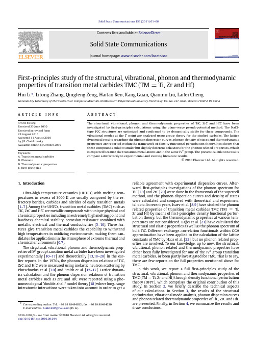
1. Introduction Ultra-high temperature ceramics (UHTCs) with melting temperatures in excess of 3000 K are usually composed by the refractory borides, carbides and nitrides of early transition metals [1–7]. Among the UHTCs, transition metal carbides (TMC) such as TiC, ZrC and HfC are metallic compounds with unique physical and chemical properties including an extremely high melting point and hardness, chemical stability, corrosion resistance combined with metallic electrical and thermal conductivities [5–10]. These features give transition metal carbides the capability to withstand high temperatures in oxidizing environments, making them candidates for applications in the atmosphere of extreme thermal and chemical environments [6,7]. The structural, vibrational, phonon and thermodynamic properties of IVb group transition metal carbides have been investigated experimentally [10–17] and theoretically [13,18–28] in the earlier reports. In the 1970s, the phonon dispersion relations of TiC, ZrC and HfC were measured using inelastic neutron scattering by Pintschovius et al. [10] and Smith et al. [15–17]. Lattice dynamics calculation and the phonon dispersion relations of transition metal carbides such as ZrC and HfC were reported using a phenomenological ‘‘double-shell’’ model theory [18] where long-range interatomic interactions were taken into account in order to get a

学术英语(理工)_Unit 4

1 辐射自然存在于我们的环境当中,一般人每秒钟都遭受着来自自然资源中15，000个粒子的辐射，而一次普通的医疗 X光检查则带有1，000亿个粒子的辐射。 2 这些材料主要通过发电厂常规运行时的少量释放物，核电站事故和放射性材料运输事故、以及放射性废料从隔离系统中泄漏而与人体发生接触的。 3 在利用现有技术预防遗传性疾病方面还有很多事可以做；如果利用核工业纳税款的1%来进一步实施这项技术，那么每一种由核工业造成的疾病中有80例遗传疾病都将得到防止。
学术英语理工
Academic English
for Science and Engineering
Unit 4 Writing a Literature Review
Unit 4 Writing a Literature Review
Unit Contents
1 Writing a literature review
and repair itself. When exposed to a large amount of radiation, the cell’s
defenses are overwhelmed. Therefore an increase in cancer in the area where radiation leakage takes place (辐射泄漏发生) often arises from
1 Writing a literature Review
Enhancing your academic language
Complete the following expressions or sentences. 1 a small breach (缺口) in the dam 2 shallow (浅的) foundation 3 implement (履行) a promise 4 the survivor(s) (幸存者) of the earthquake 5 hypothetical (假设的) situation 6 initiate (发起) a reform 7 have potential (潜力) as an artist 8 despite (不顾) their strong disagreement 9 neutralize (中和) acids 10 be in contact (联系) with each other 11 transport (运输) goods by lorry 12 the volume (大量) of exports

Simple theoretical tools for low dimension Bose gases

µ is the chemical potential, and the diﬀerential operator h0 includes the kinetic energy operator and the trapping potential U (r): h0 = − ¯2 h ∆ + U (r) 2m (1.2)
J. Phys. IV France 1 (2008)
c EDP SciXiv:cond-mat/0407118v2 [cond-mat.other] 6 Sep 2005
Simple theoretical tools for low dimension Bose gases
Pr1-2
JOURNAL DE PHYSIQUE IV
It is convenient to expand the ﬁeld operator on the orthonormal basis of the eigenmodes φα (r) of h0 with eigenenergy ǫα : ˆ(r) = ψ φα (r)ˆ aα (1.5)
so that we recover the condition for a non-degenerate regime ρλd ≪ 1. (1.17)
• degenerate regime: |µ| ≪ kB T so that the ground mode of the gas has a large occupation number: kB T ≫1 (1.18) n0 ≃ |µ| where we have expanded the exponential in the Bose law to ﬁrst order in its argument. In this case several modes have a large occupation number, as soon as |µ| ≪ kB T , because condition (1.13) holds. • the ground mode is more populated than any other mode: this regime is reached when the ground mode is more populated that the ﬁrst excited mode: n0 ≃ which results in |µ| ≪ ǫ1 . (1.20) It is the right time to recall the phenomenon of saturation of the total occupation of the excited modes, a key consequence of the Bose law: for a given temperature the maximal value of the excited modes population is N′ ≡

药名常用词尾,词首

药名常用词尾-al 醛-aldehyde 醛-amide 酰胺-amidine 脒-amine 胺-ane 烷-ase 酶-ate ①盐②酯-azide 叠氮；-N3-caine 卡因（局部麻醉药词尾）-carbonyl 羰基-carboxamide 甲酰胺-carboxylic acid 羧酸-cidin 杀……菌素-cillin 青霉素；西林（青霉素族抗生素词尾）-cycline 四环素（四环素族抗生素词尾）-diol ①二醇②二酚-dione 二酮-disulfide 二硫（化物）-ene 烯-enol 烯醇-ester 酯-flavine 黄素-form 仿（俗名词尾）-genin 甙元（旧称配基）-hydrin 醇-ine 碱；素（生物碱词尾）-lactone 内酯-lysin 溶素（俗名词尾）-micin 霉素（抗生素词尾）-mycetin 霉素；菌素（抗生素词尾）-mycin 霉素（抗生素词尾）-nitrile 腈-ol ①醇②酚-olol 心安（心安类药物词尾）-one 酮-ose 糖-oside 糖甙-oxide 氧；氧化物-oyl 酰-quine 奎（俗名尾词）-sporin 孢菌素（抗生素词尾）-sullide 硫（化物）-sulfone 砜-sulfoxide 亚砜-thioic acid 硫代酸-thione 硫酮-toxin 毒-triol 三醇-tropin 托品（俗名尾词）-urea 脲-xanthin 黄质-yl 基（一价基）-yne 炔药名常用词首ace- 乙（酰基）acet- 醋；醋酸；乙酸acetamido- 乙酰胺基acetenyl- 乙炔基acetoxy- 醋酸基；乙酰氧基acetyl- 乙酰（基）aetio- 初allo- 别allyl- 烯丙（基）；CH2=CH-CH2- amido- 酰胺（基）amino- 氨基amyl- ①淀粉②戊（基）amylo- 淀粉andr- 雄andro- 雄anilino- 苯胺基anisoyl- 茴香酰；甲氧苯酰anti- 抗apo- 阿朴；去水aryl- 芳（香）基aspartyl- 门冬氨酰auri- 金（基）；（三价）金基aza- 氮（杂）azido- 叠氮azo- 偶氮basi- 碱baso- 碱benxoyl- 苯酰；苯甲酰benzyl- 苄（基）；苯甲酰bi- 二；双；重biphenyl- 联苯基biphenylyl- 联苯基bis- 双；二bor- 硼boro- 硼bromo- 溴butenyl- 丁烯基（有1、2、3位三种）butoxyl- 丁氧基butyl- 丁基butyryl- 丁酰caprinoyl- 癸酰caproyl- 己酰calc- 钙calci- 钙calco- 钙capryl- 癸酰capryloyl- 辛酰caprylyl- 辛酰cef- 头孢（头孢菌素族抗生素词首）chlor- ①氯②绿chloro- ①氯②绿ciclo- 环cis- 顺clo- 氯crypto- 隐cycl- 环cyclo- 环de- 去；脱dec- 十；癸deca- 十；癸dehydro- 去氢；去水demethoxy- 去甲氧（基）demethyl- 去甲（基）deoxy- 去氧des- 去；脱desmethyl- 去甲（基）desoxy- 去氧dex- 右旋dextro- 右旋di- 二diamino- 二氨基diazo- 重氮dihydro- 二氢；双氢endo- 桥epi- 表；差向epoxy- 环氧erythro- 红；赤estr- 雌ethinyl- 乙炔（基）ethoxyl- 乙氧（基）ethyl- 乙基etio- 初eu- 优fluor- ①氟②荧光fluoro- ①氟②荧光formyl- 甲酰（基）guanyl- 脒基hepta- 七；庚hetero- 杂hexa- 六；己homo- 高(比原化合物多一个-CH2-)hypo- 次io- 碘indo- 碘iso- 异keto- 酮laevo- 左旋leuco- 白levo- 左旋mercapto- 巯基meso- ①不旋；内消旋②中（间）③中（位）（蒽环的9、10位）meta- ①间（有机系统用名）②偏（无机酸用）methoxy- 甲氧基methyl- 甲基mono- 一；单neo- 新nitro- 硝基nitroso- 亚硝基nona- 九；壬nor- 去甲；降；正nov- 新novo- 新oct- 八；辛octa- 八；辛octo- 八；辛ortho- ①邻（位）②正③原oxalo- 草oxo- 氧[代]oxy- ①氧②羟基（误称，但常用）para- ①对（位）②副（俗名）penta- 五；戊per- ①高②过phen- 苯pheno- 苯phenoxy- 苯氧（基）phenyl- 苯基phospho- 磷；磷酸phosphor- 磷；磷酸phosphoro- 磷；磷酸phyllo- 叶poly- 多；聚propyl- 丙基proto- 原pseudo- 假；伪；拟ribosyl- 核糖基sec- ①另（指CH3CH2CH(CH3)-型烃基②semi- 半silico- 硅strept- 链strepto- 链sulf- 硫sulfa- 磺胺（磺胺类药物词头）sulfo- ①硫[代]②磺基sulph- 硫[代]sulpho- ①硫[代]②磺基tert- ①特（指CH3…C(CH3)2-型烃基）②叔tetra- 四thio- 硫trans- 反（式）；转tri- 三undeca- 十一valyl- 缬氨酰（基）vinyl- 乙烯基xantho- 黄色药学英语缩略语词汇5-FU（5-fluorouracil）5-氟尿嘧啶5-HT（5-hydroxytryptamine，serotonin：5-羟色胺）5-羟色胺6-MP（6-mercaptopurine）6-巯基嘌呤A/G （albumin/ globin：珠蛋白；球蛋白；珠朊；血球蛋白）白球蛋白比率ACD （acid-citrate-dextrose）酸性枸橼酸葡萄糖ACP （acid phosphatase）酸性磷酸酶ACTH （Adrenocorticotropic Hormone）促肾上腺皮质激素ADH （antidiuretic hormone）抗利尿激素ADP （adenosine diphosphate）二磷酸腺苷AFP （alpha-fetoprotein）甲（种）胎（儿）蛋白AHF （antihemophilic factor）抗血友病因子AKP （alkaline phosphatase）碱性磷酸酶ALL （Acute lymphocytic leukemia）急性淋巴细胞性白血病ALS （anti lymphocyte serum）抗淋巴细胞血清ALT(GPT) （alanine aminotransferase/glutamic-pyruvic transaminase）丙氨酸转氨酶AMA （anti-mitoehondria antibody）抗线粒体抗体AMI （Acute Myocardial Infarction）急性心肌梗塞AML （Acute Myelogenous Leukemia）急性粒细胞性白血病AMP （adenosinemonophosphate）一磷酸腺苷ANA （antinuclear antibodies）抗核抗体APC （aspirin,phenacetin and caffeine compound）复方阿司匹林AST(GOT) （aspartate transaminase/glutamic-oxalacetic transaminease）天冬氨酸转氨酶ATN （acute tubular necrosis）急性肾小管坏死ATP （adenosine triphosphate）三磷酸腺苷BCG （bacillus Calmette-Guerin vaccine）卡介苗BCNU（bis-chloroethyl nitrosourea carmustine，）卡氮芥BMR （Basal metabolic rate）基础代谢率BP （blood pressure）血压BSA (1 bovine serum albumin)牛血清白蛋白；(2body surface area：体表面积；體表面積；面积；释义：人体表面积)体表面积BSP （bromsulphalein）磺溴酞钠BT （bleeding time）出血时间BUN （blood urea nitrogen）血尿素氮BV （blood volume）血容量C3 （complement-3）补体3cAMP （cyclic adenosine monophosphate）环磷酸腺苷CAPD （Continuous Ambulatory Peritoneal Dialysis）不卧床的持续性腹膜透析CB-1348 （chlorambucil）苯丁酸氮芥CBG （corticosteroid-binding globulin）皮质类固醇结合球蛋白CCNU （cyclohexyl-chloro-ethyl-nitrosourea）环己亚硝脲CCU （coronary care unit）冠心病监护病室CEA （carcinoembryonic antigen）癌胚抗原cGMP （cyclic guanosine monophosphate）环磷鸟苷CIC （circulating immune complex）循环免疫复合物CIEP （counter immunoelectrophoresis：对流免疫电泳；释义：对流免疫电泳,逆向免疫电泳）对流免疫电泳CLL （chronic lymphocytic leukemia）慢性淋巴细胞性白血病CML （Chronic myelogenous leukemia）慢性粒细胞性白血病CMV （cytomegalovirus）巨细胞病毒CNS （central nervous system）中枢神经系统CO2cp （carbon dioxide combining power）二氧化碳结合力CoA （coenzyme A）辅酶ACO （cardiac output）心输出量CPBA （competitive protein binding assay）竞争性蛋白结合分析CPC （Clinico-Pathological Conference：皮肤科临床病理讨论会）临床病理讨论会CPK （creatine phosphokinase）肌酸磷酸激酶cpm （counts per minute）每分钟计数CSF （cerebrospinal fluid）脑脊髓液CT ( Computed Tomography)电算机体层摄影CVP（Central Venous Pressure）中心静脉压DIC （disseminated intravascular coagulation）播散性血管内凝血DMSA （Dimercapto Succinic Acid）二巯基丁二酸DNA （desoxyribonucleic acid）脱氧核糖核酸DNCB （dinitrochlorobenzene）二硝基氯苯DOCA （desoxycorticosterone acetate）醋酸脱氧皮质酮dpm （disintegration per minute）每分钟衰变数DSA （digital subtraction angiography）数字减影血管造影DSS （dengue shock syndrome）登革休克综合征DTPA （diethylenetriamine pentaacetic acid）二乙三胺五乙酸ECG;EKG （electrocardiogram）心电图EDTA （Ethylene Diamine Tetraacetic Acid）乙二胺四乙酸EEG （electroencephalo-graph）脑电图EHF （epidemic hemorrhagic fiver）流行性出血热EIA （enzyme immunoassay）免疫酶法ELISA （enzyme-linked immuno sorbent assay）酶联免疫吸附试验EMCP, EMG（electromyography）肌电图ENT （ear，nose，and throat）耳鼻咽喉ERCP （Endoscopic Retrograde Cholangiopancreatography）逆行胰胆管造影ESR （erythrocyte sedimentation rate）红细胞沉降率FSH-RH （follicle stimulating hormone releasing hormone）促卵泡素释放激素FSH （Follicle-Stimulating Hormone）促卵泡素FT4I （free thyroxine index）游离甲状腺素指数FT4 （free thyroxine）游离甲状腺素GABA (γ-Aminobutyrate) γ-氨基丁酸GH （growth hormone）生长激素GTT （Glucose Tolerance Test）葡萄糖耐量试验HAI;HI （Hemagglutination-inhibition test）血凝抑制试验HA V （Hepatitis A virus）甲型肝炎病毒HBcAg （hepatitis B core antigen）乙型肝炎核心抗原HBeAg （Hepatitis B e Antigen）乙型肝炎e抗原HBsAg （epatitis B surface antigen）乙型肝炎表面抗原HBV （hepatitis B virus）乙型肝炎病毒Hb （hemoglobin）血红蛋白HCG （Human Chorionic Gonadotropin）人绒毛膜促性腺激素HCV （hepatitis C virus）丙型肝炎病毒HDL （high density lipoprotein）高密度脂蛋白HDV （hepatitis delta virus）丁型肝炎病毒HEV （Hepatitis E Virus）戊型肝炎病毒HIV （human immunodeficiency virus）人类免疫缺陷病毒HLA （human leukocyte antigen）人白细胞抗原系统HP （highpowerfield）高倍视野ICU （Intensive Care Unit）危重症病人监护病室IFA （immunoflourescence assay）免疫萤光法Ig （immunoglobulin）免疫球蛋白ITP （idiopathic thrombocytopenic purpura）特发性血小板减少性紫癜IVU （intravenous urography）静脉尿路造影JBE （Japanese B encephalitis）日本乙型脑炎LATS （long-acting thyroid stimulator）长效甲状腺刺激素LD50 （lethal dose50）半致死量LDH （lactic dehydrogenase）乳酸脱氢酶LDL （Low Density Lipoprotein）低密度脂蛋白LH-RH （Luteinizing Hormone-Releasing Hormone）黄体生成素释放激素LH （Luteinizing Hormone）黄体生成素LP （low power field）低倍视野MAA巨聚白蛋白MCHG （Mean Corpuscular Hemoglobin）平均红细胞血红蛋白浓度MCV （Mean Corpuscular V olume）平均红细胞体积MDP （methylene diphosphonic Acid）亚甲基二磷酸MRI(NMR) （Magnatic Resonance Imaging, nuclearmagnetic resonance）磁共振（核磁共振）成像MTX （methotrexate）氨甲蝶呤NHL （non-hodgkin's lymphoma）非何杰金淋巴瘤NPN （non protein nitrogen）非蛋白氮OT （old tyberculin）旧结核菌素PaCO2 （arterial partial pressure of carbon dioxide：动脉血二氧化碳分压）动脉血二氧化碳分压PAGE （polyacrylamide gel electrophoresis）聚丙烯酰胺凝胶电泳PaO2 （arterial partial pressure of oxygen）动脉血氧分压PAS （para amino salicylic acid）对氨基水杨酸PBI蛋白结合碘（protein-bound iodine）PBS （phosphate buffer solution）磷酸盐缓冲液PB （phosphate buffer）磷酸盐缓冲剂PCR （polymerase chain reaction）聚合酶链反应PG （prostaglandin）前列腺素PHA （phytohemagglutinphytolectin）植物血凝素：被动血凝试验PPD （Purified Protein Derivative）结核菌素纯蛋白衍生物PSP （phenolsulfonphthalein）酚磺酞（酚红）PTC （percutaneous transhepatic cholangiography）经皮肝穿刺胆道造影PTH （parathyroid hormone）甲状旁腺激素PT （protrombin time）凝血酶原时间RBC（red blood cell）红细胞RES （reticuloendothelial system）网状内皮系统RF （rheumatoid factor）类风湿因子RIA （radioimmunoassay）放射免疫分析RNA （Ribonucleic Acid）核糖核酸rpm （Revolutions Per Minute）每分钟转速（现改用r/min）RV （Rotavirus）轮状病毒SaO2 （Oxygen Saturation）氧饱和度SBE （subacute bacterial endocarditis）亚急性细菌性心内膜炎SLE （systemic lupus erythematosus）系统性红斑狼疮SPECT （single photon emission computedtomography）单光子发射计算机断层图像检查T3 （triiodothyronine）三碘甲状腺原氨酸T4 （thyroxine）甲状腺素TBG （thyroxine binding globulin）甲状腺素结合球蛋白TG （triglyceride/）甘油三酯Tg （thyroglobulin）甲状腺球蛋白TRH （Thyrotropin-releasing Hormone）促甲状腺激素释放激素TSH （Thyroid stimulating hormone）促甲状腺激素TTT （thymol turbidity test）麝香草酚浊度试验U （unit）单位VLDL （very low density lipoprotein）极低密度脂蛋白Wbc （white blood cell）白细胞WBC （）白细胞计数WHO （world health organization）世界卫生组织A．A．A Addition and Amendments 增补和修订Special terms for medicinal chemistryAα-helix[ˈhi:liks]absorption[əbˈsɔrpʃən, -ˈzɔrp-]吸收,；吸收过程；吸收作用distribution英[ˌdistriˈbju:ʃən]美[ˌdɪstrəˈbjuʃən] 散布, 分布metablism代谢metabolism 英[mɪˈtæbəˌlɪzəm] 美[mɪˈtæbəˌlɪzəm] 新陈代谢excretion 英[eksˈkri:ʃən] 美[ɪkˈskriʃən] 排泄,排泄物toxicity 英[tɔkˈsɪsɪti:] 美[tɑkˈsɪsɪti] 毒性,毒力ADMET studiesacyl coenzyme A-cholesterol acyltransferase 酰基辅酶A-胆固醇酰基转移酶inhibitor英[inˈhibitə] 美[ɪnˈhɪbɪtɚ] 抑制剂,抑制者ACAT inhibitors酰基辅酶A-胆固醇酰基转移酶抑制剂acetamide[æsiˈtæmaid]乙酰胺derivative 英[diˈrivətiv] 美[dɪˈrɪvətɪv] 衍生物, 派生物, 引出物acetamide derivative乙酰胺衍生物acetate 英[ˈæsiˌteit] 美[ˈæsɪˌtet] 醋酸盐；醋酸酯acetic[əˈsi:tik] acidacetone 英[ˈæsitəun] 美[ˈæsɪˌton] 丙酮acetylene 英[əˈsetili:n] 美[əˈsɛtlˌin, -ən] 乙炔,电石气acetylcholine 英[əˌsi:təlˈkəulin] 美[əˌsitlˈkoˌlin]乙酰胆碱acetylcholine receptors乙酰胆碱受体acetylcholinesterase 英[ˌæsitilkəuliˈnestəreis]美[əˌsitlˌkoləˈnɛstəˌres, -ˌrez] 乙酰胆碱酯酶acetylcholinesterase inhibitors乙酰胆碱酯酶抑制剂acetylsalicylic acid 英[əˌsi:tlˌsælɪˈsɪlɪk] 美[əˌsitlˌsælɪˈsɪlɪk] 乙酰水杨酸,阿司匹林acetylpenicillamine乙酰青霉胺Acid catalyzed ketal formation 酸催化缩酮结构acidic英[əˈsɪdɪk] 酸的，酸性的acidification使发酸,酸化,成酸性acquired immunodeficiency syndrome(AIDS)获得性免免疫综合症activation 活化，激活acylation 酰化adrenergic 英[ˌædriˈnə:dʒik] 美[ˌædrəˈnɚdʒɪk] 肾上腺素的,释放肾上腺素的adrenergic agent肾上腺素能药物adrenergic blocking agent肾上腺素能阻断剂adverse reaction 副反应affinity 亲和力alcohol 乙醇aldehyde 醛alkane 英[ˈælkein] 美[ˈælˌken]链烷alkyl 英[ˈælkil] 美[ˈælkəl] 烷基alkyl phenol 烷基酚phenol 英[ˈfi:nəl] 美[ˈfiˌnɔl, -ˌnol, -ˌnɑl] 苯酚,石碳酸al kylamine [ˌælkiləˈmi:n] 烷基胺alkylaminoketone 烷基胺酮alkylating烷基化alkylating agent 烷化剂alkylsufonamidophenethanolamine 烷基磺酰基苯乙基胺aluminum英[əˈlu:mənəm] 美[əˈlumənəm]铝amide 英[ˈæmaid] 美[ˈæmˌaɪd, -ɪd] 氨基化合物，酰胺amidification in prodrug 前药中的酰胺化amidinopenicillanic acid 咪基青霉烷酸amino acid 氨基酸amino-3-indolepropionic acid 氨基-3-吲哚丙酸aminobenzoate 氨基苯甲酸酯propionic acid英[ˌprəʊpi:ˈɔnɪk] 美[ˌpropiˈɑnɪk]丙酸butyric acid 丁酸amino-beta-hydroxybutyric acid 氨基-β羟基丁酸amino-beta-hydroxypropionic acid 氨基-β羟基丙酸amino-beta-mercaptopropionic acid 氨基-β巯基丙酸aminocephalosporanic acid 氨基头孢烷酸aminoglutaramic acid 氨基戊酰胺酸pyrazines 吡嗪aminopyrazines 氨基吡嗪，diuretic英[ˌdaijuˈreitik] 美[ˌdaɪəˈrɛtɪk] 利尿剂aminosalicylic acid [əˌmi:nəʊˌsælɪˈsɪlɪk] 美[əˌminoˌsælɪˈsɪlɪk]氨基水杨酸aminosuccinic acid氨基丁二酸，天门冬氨酸aminothiadiazole 氨基噻二唑aminomethylbenzoic acid 氨基甲基苯甲酸，氨甲苯酸amyl nitrite 亚硝酸异戊酯analgesic英[ˌænəlˈdʒi:zɪk, -sɪk] 美[ˌænəlˈdʒizɪk, -sɪk]止痛药analog 类似物analog-prodrug hybrid 类似前药杂化anesthesia英[ˌænɪsˈθi:ʒə] 美[ˌænɪsˈθiʒə]麻醉anterior pituitary hormone analogs 垂体前叶激素类似物anterior 英[ænˈtɪəri:ə] 美[ænˈtɪriɚ] 位于前部的，先前的;早期的pituitary 英[pɪˈtu:ɪˌteri:, -ˈtju:-] 美[pɪˈtuɪˌtɛri, -ˈtju-] (脑)垂体anti-leishmanial agent 抗利什曼原虫药leishmanial利什曼原虫的anti-leprosy agent 抗麻风药leprosy 英[ˈleprəsi:] 美[ˈlɛprəsi] 麻风病anti-metabolite 抗代谢药anti-protozoal agent 抗原虫药protozoal [,prəutəu'zəuəl]原生动物的，原虫的：有关原虫的或由原虫引起的anti-psychotic 抗精神病药psychotic 英[saɪˈkɔtɪk] 美[saɪˈkɑtɪk] 精神病的;患精神病的psychosis英[saɪˈkəʊsɪs] 美[saɪˈkosɪs] 精神病anti-adiposity drug 抗肥胖症药adiposity [,ædi'pɔsiti]肥胖,肥胖症,肥胖倾向anti-androgen 抗雄激素androgen 英[ˈændrədʒən] 美[ˈændrədʒən] 雄性激素(尤指睾酮), 雄性荷尔蒙anti-amebic agent 抗阿米巴药ameba 英[əˈmi:bə] 美[əˈmibə] 复数：amebae阿米巴;变形虫anti-anginal agent 抗绞痛药anginal心绞痛的,咽炎的angina 英[ænˈdʒainə] 美[ænˈdʒaɪnə,ˈændʒə-] 咽峡炎;绞痛anti-anxiety agent 抗焦虑药anxiety 英[ænˈzaiəti] 美[æŋˈzaɪɪti] 焦虑,担心, 不安；焦虑的原因；渴望, 热望anti-arthritic agent 抗关节炎药arthritis 英[ɑ:ˈθraɪtɪs] 美[ɑrˈθraɪtɪs]关节炎anti-asthmatic drug 平喘药asthmatic 英[æzˈmætɪk] 气喘的；患气喘的；发出去呼哧声的asthma 英[ˈæsmə] 美[ˈæzmə] 气喘; 哮喘antibacterial 抗细菌的antibiotics 抗生素anti-convulsant agent 抗惊厥药convulsant 英[kənˈvʌlsənt] 美[kənˈvʌlsənt]惊厥剂,发厥药convulsion 英[kənˈvʌlʃən] 美[kənˈvʌlʃən]抽搐,惊厥anti-depressant agent 抗抑郁药depressant adj.有镇静作用的n.镇静剂depression; melancholia 抑郁症anti-diabetic agent 抗糖尿病药diabetic 英[ˌdaɪəˈbetɪk] 美[ˌd aɪəˈbɛtɪk] n.糖尿病患者adj.糖尿病的diabetes 英[ˌdaɪəˈbi:tɪs, -ti:z] 美[ˌdaɪəˈbitɪs,-tiz] 糖尿病anti-diarrheal agent 抗腹泻药diarrheal腹泻，腹泻的，具腹泻特点的diarrhea 英[ˌdaɪəˈri:ə] 美[ˌdaɪəˈriə] 腹泻anti-dopaminergic drug 抗多巴胺药dopaminergic 英[ˌdəupəmiˈnə:dʒik] 美[ˌdopəməˈnɚrdʒɪk] 多巴胺能的dopamine 英[ˈdəʊpəˌmi:n] 美[ˈdopəˌmin]多巴胺anti-emetic agent 止吐药emetic 英[ɪˈmetɪk] 美[ɪˈmɛtɪk] adj.催吐的n.催吐药anti-epileptics 抗癫痫药epileptic 英[ˌepəˈleptɪk] 美[ˌɛpəˈlɛptɪk] adj.由癫痫引发的n.癫痫病患者epilepsy 英[ˈepəˌlepsi:] 美[ˈɛpəˌlɛpsi] 癫痫,羊角风anti-estrogens 抗雌激素estrogen 英[ˈestrədʒən] 美[ˈɛstrədʒən] 雌激素anti-filarial drug 抗丝虫药filarial丝虫的，属于丝虫的，丝虫引起的，指丝虫的filaria ['filɛəriə] (寄生体内的)丝虫antifungal英[ˈæntifʌŋɡəl] 美[ˌæntiˈfʌŋɡəl]抗真菌的fungus 英[ˈfʌŋɡəs] 美[ˈfʌŋɡəs] 复数fungi['fʌndʒai,'fʌŋɡai]真菌，霉菌anthelmintic 英[ˌænθelˈmintik] 美[ˌænthɛlˈmɪntɪk] adj.驱虫的n.驱虫剂,打虫药helminthic 英[helˈminθik] 美[hɛlˈmɪnθɪk]adj..肠虫的,驱虫的n.驱虫剂,杀虫药helminthagogue驱蠕虫药anti-hemophilic 抗血友病药hemophilic 英[ˌhi:məˈfilik] 美[ˌhiməˈfɪlɪk]血友病的,嗜血的hemophilia 英[ˌhi:məˈfɪlɪə] 血友病,出血不止病anti-hemorrhoidal agent 抗痔药hemorrhoidal 英[ˌheməˈrɔidəl] 美[ˌhɛməˈrɔɪdl] 痔的,直肠及肛门的hemorrhoid 英[ˈheməˌrɔɪd] 美[ˈhɛməˌrɔɪd]痔疮anti-histamine 抗组胺药anti-HIV agent 抗HIV药物antihyperlipidemic agent 抗高血酯药hypolipidemic 降血脂药hyperlipidemia 英[ˈhaipəˌlipiˈdi:miə] 美[ˌhaɪpɚˌlɪpɪˈdimiə] 血脂过多,高脂血hypolipidemia血脂过少antihypertensive agent英[ˈæntiˌhɑipəˈtensiv] 美[ˌæntiˌhaɪpɚˈtɛnsɪv]抗高血压药hypertensive 英[ˌhaipə(:)ˈtensiv] 美[ˌhaɪpɚˈtɛnsɪv] adj.高血压的n.高血压患者hypertension英[ˌhaɪpəˈtenʃən] 美[ˌhaɪpɚˈtɛnʃən] 高血压hypotension 英[ˌhaipəuˈtenʃən] 血压过低anti-infectives 抗感染药anti-inflammatory agent 抗炎药anti-inhibitor coagulant complex 抗抑制剂促凝剂复合物coagulant 英[kəʊˈægjələnt] 美[koˈæɡjələnt] 凝结剂antilipemic agent 抗高血脂药lipaemia 脂血;脂血症anti-malarial 抗疟药malarial [mə'lɛəriəl]疟疾的malaria 英[məˈlɛəriə] 美[məˈlɛriə] 疟疾anti-metabolites 抗代谢药metabolite 英[miˈtæbəlait]美[mɪˈtæbəˌlaɪt] 代谢物metabolic 1.代谢作用的,新陈代谢的 2.变化的;新陈代谢的metabolism 英[mɪˈtæbəˌlɪzəm] 美[mɪˈtæbəˌlɪzəm] n. 新陈代谢metabolize 英[mɪˈtæbəˌlaɪz] 美[mɪˈtæbəˌlaɪz] vt.使发生新陈代谢antimigraine，anti-migraine drug，抗偏头痛药migraine 英[ˈmaɪˌgreɪn] 美[ˈmaɪˌɡren] 偏头痛anti-oxidant 抗氧化剂antipyretic英[ˌæntipaiˈretik] 美[ˌæntipaɪˈrɛtɪk] adj.退热的, 退烧的n.退热药pyretic 英[paiˈretik] 美[paɪˈrɛtɪk] 发烧的,热病的,引起发烧的pyrexia 英[paiˈreksiə] 美[paɪˈrɛksiə] 发热,热病antiretroviral agent 抗逆转录病毒药retrovirus 英[ˌretrəuˈvaiərəs] 美[ˌrɛtroˈvaɪrəs, ˈrɛtrəˌvaɪ-]逆转录酶病毒anti-rheumatics 抗风湿药rheumatic [ru:'mætik, ru-] adj. 风湿病的；风湿病引起的n. 风湿病；风湿病患者antischistosomal drug 抗血吸虫药schistosome ['ʃistəsəum, 'skjtə-] n. 血吸虫；裂体吸虫antiseptics [,ænti'septiks] 防腐剂anti-spasmodic agent 解痉药spasmodic[spæz'mɔdik] adj. 痉挛的，痉挛性的；间歇性的antithrombotics 抗血栓形成药antithrombotic ['ænti,θrɔm'bɔtik] adj. 【医学】抗血栓形成的，抗血栓的antithyroid agent抗甲状腺药antithyroid ['ænti'θairɔid] adj. 抗甲腺的n. 抗甲腺药剂thyroid ['θairɔid] n. [解]甲状腺；甲状软骨；甲状腺剂adj. [解]甲状腺的；盾状的anti-trematodes抗吸虫药trematodes n. 吸虫（trematode的复数形式）；吸虫类anti-trichomonal 抗毛滴虫药trichomonal [,trikəu'mɔnəl] adj.(关于)毛滴虫的；由毛滴虫引起的antituberculous agent 抗结核药tuberculous [tju:'bə:kjuləs] adj. 结节状的；有结节的；患结核病的antitussive [,ænti'tʌsiv] n. 止咳药adj. 能止咳的antiulcer agent[,ænti'ʌlsə] 抗溃疡药anti-varicose drug 抗静脉曲张药varicose ['værikəus] adj. 静脉曲张的；曲张的，肿胀的antiviral agent 抗病毒药anxiolytics 抗焦虑药anxiolytic [æŋ,zaiə'litik] n. 抗焦虑药adj. 抗焦虑的arylacetic acid derivative 芳基乙酸衍生物aryl ['æril] adj. 芳基的n. 芳基arylalkylamine 芳基烷胺alkylamine [,ælkilə'mi:n] n. 烷基胺ascorbic acid [ə'skɔ:bik]抗坏血酸ascorbyl palmitate 抗坏血酸棕榈酸酯Bβ-lactamase β-内酰胺酶lactamase ['læktəmeis] n. [生化]内酰胺酶basic 碱性的benzimidazole [,benzimi'dæzəul]苯并咪唑benzoaldehyde 苯甲醛benzodiazepine英[ˌbenzəʊdaɪˈæzəˌpi:n] 美[ˌbɛnzodaɪˈæzəˌpin]苯丙二氮benzofuran [,benzəu'fjuəræn]苯并呋喃，香豆酮benzoic acid 苯甲酸benzophenone [,benzəu'finəun] n. 苯甲酮,二苯甲酮benzoylperoxide 过氧化苯甲酰benzquinamide 苯喹胺（止吐药）dichloracetic acid 二氯乙酸bicyclic compound 二环化合物bioactivation 生物活性bioinformatics 生物信息学biological membrane 生物膜biotransformation 生物转化biphenylacetic acid 联苯乙酸β-lactam antibiotics β-内酰胺抗生素bulky group 空间障碍基团bond-covalent 共价键bond-dipole 偶极键bond-hydrogen 氢键bond-ion-dipole 离子偶极键bond-ionic 离子键bretylium tosylate [bri'tiljəm'təusileit] 溴苯胺（降压药）broat-spectrum antibacterial agent 广谱抗菌剂bromide 溴化物buffer 缓冲剂butoxyethyl nicotinate 烟酸丁氧乙基酯Ccalcium channel blocker 钙通道阻滞剂cncer chemotherapy 癌症化疗crbohydrate metabolism drug 碳水化合物代谢药carbutamide 磺胺丁脲cardiac glycoside 强心甙cardiovascular agent 心血管药central nervous system 中枢神经系统cephalosporanic acid 头孢烷酸cephalosporin [,sefələ'spɔ:rin]头孢菌素channel blocker 通道阻断剂channel former通道离子载体，通道构象charge densities 电荷密度charge transfer 电荷转移chelating 螯合chelate ['ki:leit] n. [化]螯合物adj.螯合的；有螯的vt. 与（金属）结合成螯合物chelating agent 螯合剂chemical name 化学名chemical structure 化学结构chemotherapeutic化疗的chemoreceptor trigger zone 化合受体触发区域chiral center ['kaiərəl] 手性中心chloramphenicol [,klɔ:ræm'fenikɔl]氯霉素chloride 氯化物cholinomimetic [,kəulinəumi'metik]拟胆碱作用的chromic chloride 氯化铬combinatorial peptide synthesis 组合肽合成combinatorial [kɔm,bainə'tɔ:riəl] adj. 组合的competitive antagonist 竞争性拮抗剂complementarity between drug and receptor药物受体之间互补compound 化合物configuration 构型conformation 构象congener ['kɔndʒinə]同族元素conjugation [,kɔndʒu'ɡeiʃən]共轭conjugative effect 协同效应coumarin ['ku:mərin] n. [化]香豆素cyclohexanone [,saikləu'heksənəun]环己酮cyclophosphamide [,saikləu'fɔsfəmaid]环磷酰胺cytokines 细胞因子DDDC coupling reagent DDC偶联试剂dealkylation [di:ælki'leiʃən]去烷基化deamination [di:,æmi'neiʃən] n. [化]去氨基；脱氨基作用dehalogenation [di:hælədʒəneiʃən] n. [化]脱卤酌；[化]脱卤作用；去卤化dichlorotetrafluoroethane二氯四氟乙烷diphenylpropylamines and isosteres 联苯基丙胺及异构体diphenyl [daifenil] n. [化]联苯；[医]二苯基propylamine 丙胺disulfide 二硫化物diuretic [,daijuə'retik] adj. 利尿的n. 利尿剂DNA probes DNA探针dopamine 多巴胺double esters 二酯drug-parasite-host relationship 药物、寄生虫和宿主关系Eelectron charge distribution 电子电荷的分布electron affinity 电子亲和力electronic charge density 电荷密度electronic distribution 电子分布electronic polarizability 电极化electronic states 电状态electrophilic 亲电性的empirical electronic parameter 经验电参数endogenous substance 内源性物质enzyme inhibition 酶抑制epidermal growth factor 表皮生长因子epimerization [,epimərai'zeiʃən]差向异构化epinephrine[,epi'nefrin] n. [生化]肾上腺素epoxide [i'pɔksaid]环氧化合物esterification [eʃ,steri,fi'keiʃən] n. 酯化（作用）estradiol [,estrə'daiəl] n. [化]强力求偶素，雌二醇ether ['i:θə] n. 乙醚，醚ethyl 乙基ethylenediamine [,eθili:n,daiə'mi:n, -min] n.乙二胺Ffluoroacetamide[fluərəuə'setəmaid] n. [化]氟乙酰胺；敌蚜胺（可用作杀虫剂）food additives 食物添加剂formaldehyde 甲醛formate 甲酸盐forensic 取证free valence 游离价frontier electron density 前沿电荷密度GGABA （Gamma-Amino-Butyric Acid）γ-氨基丁酸genetic polymorphism 遗传多态性general structure 一般结构genome 基因组genomics[dʒə'nəumiks] n. 基因组学；基因体学germ cell 生殖细胞glucose 葡萄糖glycinate 甘氨酸盐glycoside 糖苷group 基团Hhaloacetamide 乙酰胺盐halogen ['hælədʒin] n. 卤素halogenation [,hælədʒi'neiʃən]卤化hammett’s constant Hammett 比常数Hansh’s equation 汉施方程hair growth stimulant 毛发生长刺激剂heteroarylacetic acid 杂环芳基乙酸heterocyclic compound 杂环化合物heterocyclic isosteres 杂化异构体highest occupied molecular 最高占有分子histamine 组胺homology modeling同源性模型HOMO（highest occupied molecular orbital）最高能量占有轨道Hueckel molecular orbital Hueckel 分子轨道hybrid 杂化物hybrid substances 杂化物hybridization 杂交hydrazine ['haidrəzi:n,] n. [化]肼；肼基；[化]联氨；[化]酰肼；hydrochloric acid 盐酸hydrochlorothiazide ['haidrəu,klɔ:rə'θaiəzaid]氢氯噻嗪；二氢氯噻；双氢克尿噻hydriodic acid [,haidri'ɔdik]氢碘酸hydrophilia亲水性；吸水性hydrophobic [,haidrəu'fəubik] interaction疏水作用hydrophobicity constant 疏水性常数hydroxide 氢氧化合物hydroxy-（前缀）羟基hydroxyl group羟基hydroxylamine 羟胺hydroxylation 羟基化hydroxypropyl 羟丙基hydroxyurea [hai,drɔksi'juəriə] 羟基脲hypochlorites [,haipəu'klɔ:rait] n. [化]次氯酸盐；[化]低氧化氯IImidazole[,imi'dæzəul] n. 咪唑；异吡唑Imidazoline 咪唑啉Immunomodulator [,imjunəu'mɔdjuleitə] 免疫调制剂Immunostimulant [,imjunəu'stimjulənt] drug免疫刺激剂indolylalkylamine alkaloid吲哚基烷基胺类生物碱indole 英[ˈindəul] 美[ˈɪnˌdol] 吲哚insecticide 杀虫剂interatomic distance 原子间距intrinsic activity 内在活性isobutoic acid 异丁酸iodine 碘ion-exchange resin 离子交换树脂ionization 离子化iron 铁isobutyltriphenyl butylamine 异丁基三苯基丁胺isomer 异构体isoprofen 异布洛芬isosteres 异构体isosterism 异构化JJournals on medicinal chemistry 药物化学杂志Llatentiation 潜伏化linear free energy model 线性自由能模型lipid solubility of absorption 吸收的脂溶性lipophilicity 亲脂性liposolubility 脂溶性lowest empty molecular orbital 最低能量空轨道Mmacrolide antibiotics 大环内酯抗生素macromolecular 大分子的mechanism of action 作用机制mercaptopurine 巯基嘌呤metal 金属methyl 甲基methylchromone 甲基色酮methyldopa 甲基多巴methyl hexylamine，methylhexaneamine 甲基己胺modeling 模拟models of action 作用模型mol 摩尔molar 摩尔的molecular modification 分子修饰muscarine ['mʌskərin, -ri:n] 毒蝇碱；蕈毒碱；腐鱼毒muscle relaxant 肌肉松弛剂mutual prodrug 协同前药Nnasal decongestant 鼻黏膜充血消除药nervous system 神经系统net electronic charge 静电荷nicotinamide [,nikə'tinəmaid]烟酰胺nicotinate 烟酸酯（盐）nitrate ester 硝酸酯nitric acid 硝酸nitriles，nitrile ['naitrail] n. [化]腈，腈类nitro 硝基nitrogen 氮气nitrogen mustard 氮芥nitroheterocyclic derivatives 硝基杂环衍生物nitrous oxide 氧化亚氮nitrobenzamide 硝基苯甲酰胺nondepolarizing 非去极化non-specific drug 非特异性药non-steroidal and anti-inflammatory agent 非甾体抗炎药norepinephrine [,nɔ:repi'nefrin]去甲肾上腺素nuclear magnetic resonance（NMR）核磁共振Ooccupancy theory 占有理论octanoic acid 辛酸oligonucleotide 寡核苷酸optimization 优化organic iodine 有机碘organometallic compound 有机金属化合物organophosphates 有机磷酸盐orphan drug 罕见病用药oxidation 氧化oxide 氧化物oxide formation 氧化物生成oxidizing agent 氧化剂oxygen 氧Ppalmitate['pælmiteit] [化]棕榈酸酯；[化]棕榈酸盐paraformaldehyde [,pærəfɔ:'mældəhaid]多聚甲醛parameter 参数penicillamine 青霉胺perchlorate 高氯酸盐permanganate 高锰酸盐peroxide 过氧化物pharmaceutical 制药的pharmacophoric moieties 药效团的部分phenol 苯酚phenothiazine 吩噻嗪phenylacetic acid 苯乙酸phenylalkylamine 苯烷胺phenylbutyric acid 苯基丁酸phenylethyl alcohol 苯乙醇phosphate 磷酸盐phosphoric acid 磷酸phosphorylation agent 磷酰化剂physicochemical properties 理化性质physiological 生理的piperazine [pi'perəzi:n] [化]哌嗪；[医]胡椒嗪piperazinedione 哌嗪二酮piperidione 哌啶二酮polarizability 极化polyethylene 聚乙烯polymer 多聚体polystyrene sulfonate 硫酸聚苯乙烯polyvinyl 聚乙烯的potassium 钾prodrug 前药propanediol [prə'pænədiəul] 丙二醇propionic acid 丙酸protease inhibitor 蛋白酶抑制剂psychoactive[ˌsaɪkəʊˈæktɪv] agent 对精神起显著作用药pump 泵purified 纯净的pyrazinamide [,pirə'zinəmaid]吡嗪酰胺QQSAR （Quantitative Structure-activityRelationship）定量构效关系quaternary ammonium 季胺quinazoline [kwi'næzəli:n] n. 间二氮杂萘；喹唑啉quinidine['kwinidi:n] 奎尼丁；奎尼定（抗心律不齐药）quinolone ['kwinələun] 喹诺酮Rrandom screening in drug discovery 药物发现的随机筛选rare erath metal 稀有土金属rational approach in drug design 药物设计的合理途径rational design 合理设计recptor 受体reversible 可逆的ring closing or opening 闭环或开环Ssalicyl alcohol 水杨醇salicylate [sæ'lisileit] n. [化]水杨酸盐salicylic acid 水杨酸selenium sulfide 硫化硒semi-synthetic 半合成的sequence homology 序列同源性signal transduction 信号传导silica gel 硅胶silicon compound 硅化物silicon dioxide 二氧化硅silver nitrate 硝酸银simplification 简化slow channel 慢道soft drugs 软药solubilizing agent 增溶剂solvent 溶剂sorbic acid 山梨醇specificity 特异性spectrum of activity 作用谱（作用范围）stability 稳定性stereochemistry of acetylcholine 乙酰胆碱立体化学steroid 甾体streptomycin 链霉素structure-activity relationship 构效关系sublimed sulfur 升华硫succinonitrile 琥珀腈sulfide 硫化物sulfonamides 磺酰胺类sulfone 砜sulfonic acid 磺酸sulfonylureas[,sʌlfənil'juəriə] 磺酰脲类（治糖尿病的口服药，等于sulphonylurea）sulfur 硫sunscreen防晒surfactant 表面活性剂synthesis 合成Ttarget 靶标tartaric acid 酒石酸tetracycline 四环素thermodynamic activity 热力学活性thienamycin 硫霉素thiol 巯基three-dimensional structure 三维结构thromboxane 血栓素topical 表面的trichloroethylene 三氯乙烯tricyclic 三环的triphenylmethane 三苯甲烷Uunsaturated 不饱和urea 脲Vvapor pressure 蒸气压vectors 载体vasodilator 血管扩张剂vinylpyrimidine 乙烯嘧啶viral vector 病毒载体Wwater for injection 注射用水water for irrigation 冲洗用水white lotion 白色洗液white ointment 白色软膏XX-ray diffraction X射线衍射xylose 木糖Yyellow ferric oxide 黄色氧化铁zzinc 锌Special terms for pharmaceuticsAabsolute bioavailability 绝对生物利用度absorption 吸收acacia gum 阿拉伯胶accelerated stability 加速稳定性试验accumulation factor 蓄积因子activated charcoal 活性炭additives 附加剂adverse reaction 不良反应aerosil ['ɛərəsil]微粉硅胶aerosol ['εərəsɔl] n. 气溶胶；气雾剂；喷雾器；浮质adj. 喷雾的；喷雾器的affinity 亲和力agar 琼脂agglomeration [ə,ɡlɔmə'reiʃən] 凝聚；结块；成团；复聚aggregation 聚集（作用）air suspension coatingalbumin ['ælbjumin] n. 白蛋白，清蛋白alginate['ældʒineit] n. 藻朊酸盐海藻酸盐alginic [æl'dʒinik] acid海藻酸amorphous [ə'mɔ:fəs] adj. 无定形的；无组织的；非晶形的amorphous form 无定形amphiphilic[,æmfi'filik] adj. [生化]两亲的；[生化]两性分子的ampoule['æmpju:l] n. [医]安瓿（等于ampul）angle of friction 摩擦角angle of repose 休止角anhydrous lanolin 无水羊毛脂anion ['ænaiən] [化]阴离子。

1、下载文档前请自行甄别文档内容的完整性，平台不提供额外的编辑、内容补充、找答案等附加服务。
2、"仅部分预览"的文档,不可在线预览部分如存在完整性等问题,可反馈申请退款(可完整预览的文档不适用该条件!)。
3、如文档侵犯您的权益，请联系客服反馈,我们会尽快为您处理(人工客服工作时间：9:00-18:30)。