Detection of Nine M8.0-L0.5 Binaries The Very Low Mass Binary Population and its Implicatio
使用计算机视觉技术进行多目标追踪的常用软件介绍
使用计算机视觉技术进行多目标追踪的常用软件介绍多目标追踪是计算机视觉领域的研究热点之一,它的目标是实时且准确地识别和跟踪图像或视频中的多个目标。
在处理复杂的场景中,多目标追踪可以广泛应用于视频监控、智能交通、无人驾驶、人机交互等领域。
为了实现高效的多目标追踪,有许多常用软件可以用来辅助实现这一任务。
1. OpenCV (Open Source Computer Vision Library)OpenCV是一种广泛使用的计算机视觉库,提供了许多用于多目标追踪的函数和工具。
它支持多种编程语言,如C++、Python和Java,具有跨平台特性,在Windows、Linux和MacOS等操作系统上可用。
OpenCV提供了各种算法和技术来实现多目标追踪。
其中,基于颜色空间的背景减除算法、卡尔曼滤波器和相关滤波器等被广泛用于跟踪目标。
此外,OpenCV还提供了一些预训练的目标检测器和跟踪器,如Haar分类器、HOG(Histogram of Oriented Gradients)和CSRT(Channel and Spatial Reliability Tracking)等。
2. Tensorflow Object Detection APITensorflow Object Detection API是谷歌公司推出的一个开源项目,旨在简化目标检测和追踪任务的开发。
该API提供了一系列预训练的深度学习模型,如FasterR-CNN、SSD(Single Shot MultiBox Detector)和YOLO(You Only Look Once)等,这些模型可以用于目标检测和多目标追踪。
Tensorflow Object Detection API支持多种架构和模型的选择。
用户可以根据自己的需求选择适合的模型,并进行相应的调整和优化。
此外,该API还提供了一些用于数据预处理、模型训练和推理的工具和功能,使得实现多目标追踪变得更加便捷和高效。
计算机其它_PETS2009BenchmarkData(PETS2009基准数据集)

PETS 2009 Benchmark Data(PETS 2009基准数据集)数据摘要:The datasets are multisensor sequences containing different crowd activities.The aim of this workshop is to employ existing or new systems for the detection of one or more of 3 types of crowd surveillance characteristics/events within a real-world environment. The scenarios are filmed from multiple cameras and involve up to approximately forty actors.More specifically, the challenge includes estimation of crowd person count and density, tracking of individual(s) within a crowd, and detection of flow and crowd events.中文关键词:跟踪,事件检测,拥挤人群,人员计数,人群密度,PETS 2009,英文关键词:tracking,event detection,crowd person,count,person density,PETS 2009,数据格式:TEXT数据用途:The aim of this workshop is to employ existing or new systems for the detection of one or more of 3 types of crowd surveillance characteristics/events within a real-world environment.数据详细介绍:PETS 2009 Benchmark DataOverviewThe datasets are multisensor sequences containing different crowd activities. Please e-mail *********************if you require assistance obtaining these datasets for the workshop.Aims and ObjectivesThe aim of this workshop is to employ existing or new systems for the detection of one or more of 3 types of crowd surveillance characteristics/events within a real-world environment. The scenarios are filmed from multiple cameras and involve up to approximately forty actors. More specifically, the challenge includes estimation of crowd person count and density, tracking of individual(s) within a crowd, and detection of flow and crowd events.News06 March 2009: The PETS2009 crowd dataset is released.01 April 2009: The PETS2009 submission details are released. Please see Author Instructions.PreliminariesPlease read the following information carefully before processing the dataset, as the details are essential to the understanding of when notification of events should be generated by your system. Please check regularly for updates. Summary of the Dataset structureThe dataset is organised as follows:Calibration DataS0: Training Datacontains sets background, city center, regular flowS1: Person Count and Density Estimationcontains sets L1,L2,L3S2: People Trackingcontains sets L1,L2,L3S3: Flow Analysis and Event Recognitioncontains sets Event Recognition and Multiple FlowEach subset contains several sequences and each sequence contains different views (4 up to 8). This is shown in the diagram below:Calibration DataThe calibration data (one file for each of the 8 cameras) can be found here. The ground plane is assumed to be the Z=0 plane. C++ code (available here) is provided to allow you to load and use the calibration parameters in your program (courtesy of project ETISEO). The provided calibration parameters were obtained using the freely available Tsai Camera Calibration Software by Reg Willson. All spatial measurements are in metres.The cameras used to film the datasets are:view Model Resolution frame rate Comments001 A xis 223M 768x576 ~7 Progressive scan002 A xis 223M 768x576 ~7 Progressive scan003 P TZ Axis 233D 768x576 ~7 Progressive scan004 P TZ Axis 233D 768x576 ~7 Progressive scan005 S ony DCR-PC1000E 3xCMOS 720x576 ~7 ffmpeg De-interlaced 006 S ony DCR-PC1000E 3xCMOS 720x576 ~7 ffmpeg De-interlaced 007 C anon MV-1 1xCCD w 720x576 ~7 Progressive scan008 C anon MV-1 1xCCD w 720x576 ~7 Progressive scanFrames are compressed as JPEG image sequences. All sequences (except one) contain Views 001-004. A few sequences also contain Views 005-008. Please see below for more information.OrientationThe cameras are installed at the locations shown below to cover an approximate area of 100m x 30m (the scale of the map is 20m):The GPS coordinates of the centre of the recording are: 51°26'18.5N 000°56'40.00WThe direct link to the Google maps is as follows: Google MapsCamera installation points are shown above and sample frames are shown below:view 001 view 002 view 003 view 004view 005 view 006 view 007 view 008SynchronisationPlease note that while effort has been made to make sure the frames from different views are synchronised, there might be slight delays and frame drops in some cases. In particular View 4 suffers from frame rate instability and we suggest it be used as a supplementary source of information. Please let us know if you encounter any problems or inconsistencies.DownloadDataset S0: Training DataThis dataset contains three sets of training sequences from different views provided to help researchers obtain the following models from multiple views: Background model for all the cameras. Note that the scene can contain people or moving objects. Furthermore, the frames in this set are not necessarily synchronised. For Views 001-004 Different sequences corresponding to the following time stamps: 13-05, 13-06, 13-07, 13-19, 13-32, 13-38, 13-49 are provided. For views 005-008 (DV cameras) 144 non-synchronised frames are provided.Includes random walking crowd flow. Sequence 9 with time stmp 12-34 using Views 001-008 and Sequence 10 with timestamp 14-55 using Views 001-004. Includes regular walking pace crowd flow. Sequences 11-15 with timestamps 13-57, 13-59, 14-03, 14-06, 14-29 and for Views 001-004.DownloadBackground set [1.8 GB]City center [1.8 GB]Regular flow [1.3 GB]Dataset S1: Person Count and Density EstimationThree regions, R0, R1 and R2 are defined in View 001 only (shown in the example image). The coordinates of the top left and bottom right corners (in pixels) are given in the following table.Region Top-left Bottom-rightR0 (10,10) (750,550)R1 (290,160) (710,430)R2 (30,130) (230,290)Definition of crowd density (%): crowd density is based on a maximum occupancy (100%) of 40 people in 10 square metres on the ground. One person is assumed to occupy 0.25 square metres on the ground.Scenario: S1.L1 walkingElements: medium density crowd, overcastSequences: Sequence 1 with timestamp 13-57; Sequence 2 with timestamp 13-59. Sequences 1-2 use Views 001-004.Subjective Difficulty: Level 1Task: The task is to count the number of people in R0 for each frame of the sequence in View 1 only. As a secondary challenge the crowd density in regions R1 and R2 can also be reported (mapped to ground plane occupancy, possibly using multiple views).Download [502 MB]Sample Frames:Scenario: S1.L2 walkingElements: high density crowd, overcastSequences: Sequence 1 with timestamp 14-06; Sequence 2 with timestamp 14-31. Sequences 1-2 use Views 001-004.Subjective Difficulty: Level 2Task: This scenario contains a densely grouped crowd who walk from onepoint to another. There are two sequences corresponding timestamps 14-06 and 14-31.The task related to timestamp 14-06 is to estimate the crowd density in Region R1 and R2 at each frame of the sequence.The designated task for the sequence Time_14-31 is to determine both the total number of people entering through the brown line from the left side AND the total number of people exiting from purple and red lines, shown in the opposite figure, throughout the whole sequence. The coordinates of the entry and exit lines are given below for reference.Line Start EndEntry : brown (730,250) (730,530)Exit1 : red (230,170) (230,400)Exit2 : purple (500,210) (720,210)Download [367 MB]Sample Frames:Scenario: S1.L3 runningElements: medium density crowd, bright sunshine and shadows Sequences: Sequence 1 with timestamp 14-17; Sequence 2 with timestamp 14-33. Sequences 1-2 use Views 001-004.Subjective Difficulty: Level 3Task: This scenario contains a crowd of people who, on reaching a point in the scene, begin to run. The task is to measure the crowd density in Region R1 at each frame of the sequence.Download [476 MB]Sample Frames:Dataset S2: People TrackingScenario: S2.L1 walkingElements: sparse crowdSequences: Sequence 1 with timestamp 12-34 using Views 001-008 except View_002 for cross validation (see below).Subjective Difficulty: L1Task: Track all of the individuals in the sequence. If you undertake monocular tracking only, report the 2D bounding box location for each individual in the view used; if two or more views are processed, report the 2D bounding box location for each individual as back projected into View_002 using the camera calibration parameters provided (this equates to a leave-one-out validation). Note the origin (0,0) of the image is assumed top-left. Validation will be performed using manually labelled ground truth.Download [997 MB]Sample Frames:Scenario: S2.L2 walking Elements: medium density crowd Sequences: Sequence 1 with timestamp 14-55 using Views 001-004. Subjective Difficulty: L2Task: Track the individuals marked A and B (see figure) in the sequence and provide 2D bounding box locations of the individuals in View_002 which will be validated using manually labelled ground truth. Note the origin (0,0) of the image is assumed top-left. Note that individual B exits the field of view and returns toward the end of the sequence.Download [442 MB]Scenario: S2.L3 WalkingElements: dense crowdSequences: Sequence 1 with timestamp 14-41 using Views 001-004. Subjective Difficulty: L3Task: Track the individuals marked A and B in the sequence and provide 2D bounding box information in View_002 for each individual which will be validated using manually labelled ground truth.Download [259 MB]Dataset S3: Flow Analysis and Event RecognitionScenario: S3.Multiple FlowsElements: dense crowd, runningSequences: Sequences 1-5 with timestamps 12-43 (using Views 1,2,5,6,7,8) , 14-13, 14-37, 14-46 and 14-52. Sequences 2-5 use Views 001-004. Subjective Difficulty: L2Task: Detect and estimate the multiple flows in the provided sequences, mapped onto the ground plane as a occupancy map flow. Further details of the exact task requirements are contained under Author Instructions. These would be compared with ground truth optical flow of major flows in the sequences on the ground plane.Download [760 MB]Sample Frames:Scenario: S3.Event RecognitionElements: dense crowdSequences: Sequences 1-4 with timestamps 14-16, 14-27, 14-31 and 14-33. Sequences 1-4 use Views 001-004.Subjective Difficulty: L3Task: This dataset contains different crowd activities and the task is to provide a probabilistic estimation of each of the following events: walking, running, evacuation (rapid dispersion), local dispersion, crowd formation and splitting at different time instances. Furthermore, we are interested in systems that can identify the start and end of the events as well as transitions between them. Download [1.2 GB]Sample Frames:Additional InformationThe scenarios can also be downloaded from ftp:///pub/PETS2009/ (use anonymous login). Warning: ftp:// is not listing files correctly on some ftp clients. If you experience problems you can connect to the http server at /PETS2009/.Legal note: The video sequences are copyright University of Reading and permission is hereby granted for free download for the purposes of the PETS 2009 workshop and academic and industrial research. Where the data is disseminated (e.g. publications, presentations) the source should be acknowledged.数据预览:点此下载完整数据集。
Malnutrition Universal Screening Tool

‘MUST’is a five-step screening tool to identify adults,who are malnourished,at risk of malnutrition (undernutrition),or obese.It also includes management guidelines which can be used to develop a care plan.It is for use in hospitals,community and other care settings and can be used by all care workers.This guide contains:A flow chart showing the 5steps to use for screening and management BMI chart Weight loss tablesAlternative measurements when BMI cannot be obtained by measuring weight and height.Please refer to The ‘MUST’Explanatory Booklet for more information when weight and height cannot be measured,and when screening patient groups in which extra care in interpretation is needed (e.g.those with fluid disturbances,plaster casts,amputations,critical illness and pregnant or lactating women).The booklet can also be used for training.See The ‘MUST’Report for supporting evidence.Please note that ‘MUST’has not been designed to detect deficiencies or excessive intakes of vitamins and minerals and is of use only in adults.The 5Step 1Measure height and weight to get a BMI score using chart provided.If unable to obtain height and weight,use the alternative procedures shown in this guide.Step 2Note percentage unplanned weight loss and score using tables provided.Step 3Establish acute disease effect and score.Step 4Add scores from steps 1,2and 3together to obtain overall risk of malnutrition.Step 5Use management guidelines and/or local policy to develop care plan.Malnutrition Advisory Group A Standing Committee of BAPENM A G'Malnutrition Universal Screening Tool'B A P E NAdvancing Clinical NutritionBAPEN is registered charity number ©BAPENStep 1–BMI score (&BMI)Height (feet and inches)Weight (stones and pounds)W e i g h t (k g )Height (m)Note :The black lines denote the exact cut off points (30,20and 18.5kg/m 2),figures on the chart have been rounded to the nearest wholenumber.©BAPENStep 1BMI score+Step 2Weight loss scoreStep 3Acute disease effect score+0Low Risk1Medium Risk2or more High RiskStep 5Management guidelinesObserveDocument dietary intake for 3daysIf adequate –little concern and repeat screening Hospital –weeklyCare Home –at least monthly Community –at least every 2-3months If inadequate –clinical concern –follow local policy,set goals,improve and increase overall nutritional intake,monitor and review care plan regularlyTreat *Refer to dietitian,Nutritional Support Team or implement local policySet goals,improve and increase overall nutritional intake Monitor and review care plan Hospital –weekly Care Home –monthly Community –monthly*Unless detrimental or no benefit is expected from nutritional support e.g.imminent death.If unable to obtain height and weight,see reverse for alternative measurements and use of subjective criteriaAcute disease effect is unlikely to apply outside hospital.See ‘MUST’Explanatory Booklet for further informationStep 4Overall risk of malnutritionAdd Scores together to calculate overall risk of malnutritionScore 0Low Risk Score 1Medium Risk Score 2or more High RiskRe-assess subjects identified at risk as they move through care settingsSee The ‘MUST ’Explanatory Booklet for further details and The ‘MUST ’Report for supporting evidence.All risk categories:Treat underlying condition and provide help and advice on food choices,eating and drinking when necessary.Record malnutrition risk category.Record need for special diets and follow local policy.Obesity:Record presence of obesity.For those with underlying conditions,these are generally controlled before the treatment of obesity.BMI kg/m2Score >20(>30Obese)=018.5-20=1<18.5=2%Score <5=05-10=1>10=2Unplanned weight loss in past 3-6months If patient is acutely ill andthere has been or is likelyto be no nutritional intake for >5daysScore 2Routine clinical careRepeat screening Hospital –weeklyCare Homes –monthly Community –annually for special groups e.g.those >75yrsStep2–Weight loss score©BAPENIf height cannot be measuredUse recently documented or self-reported height (if reliable and realistic).If the subject does not know or is unable to report their height,use one of the alternative measurements to estimate height (ulna,knee height or demispan).If recent weight loss cannot be calculated,use self-reported weight loss (if reliable and realistic).If height,weight or BMI cannot be obtained,the following criteria which relate to them can assist your professional judgement of the subject’s nutritional risk category.Please note,these criteria should be used collectively not separately as alternatives to steps 1and 2of ‘MUST’and are not designed toassign a score.Mid upper arm circumference (MUAC)may be used to estimate BMI category in order to support your overall impression of the subject’s nutritional risk.1.BMIClinical impression –thin,acceptable weight,overweight.Obvious wasting (very thin)and obesity (very overweight)can also be noted.2.Unplanned weight lossClothes and/or jewellery have become loose fitting (weight loss).History of decreased food intake,reduced appetite or swallowing problems over 3-6months and underlying disease or psycho-social/physical disabilities likely to cause weight loss.3.Acute disease effectAcutely ill and no nutritional intake or likelihood of no intake for more than 5days.Further details on taking alternative measurements,special circumstances and subjective criteria can be found in The ‘MUST’Explanatory Booklet .A copy can be downloaded at orpurchased from the BAPEN office.The full evidence-base for ‘MUST’is contained in The ‘MUST’Report and is also available for purchase from the BAPEN office.BAPEN Office,Secure Hold Business Centre,Studley Road,Redditch,Worcs,B987LG.Tel:01527457850.Fax:01527458718.bapen@ BAPEN is registered charity number ©BAPEN 2003ISBN 1899467904Price £2.00All rights reserved.This document may be photocopied for dissemination and training purposes as long as the source is credited and recognised.Copy may be reproduced for the purposes of publicity and promotion.Written permission must be sought from BAPEN if reproduction or adaptation is required.If used for commercial gain a licence fee may be required.Alternative measurements and considerations©BAPEN.First published May 2004by MAG the Malnutrition Advisory Group,a Standing Committee of BAPEN.Reviewed and reprinted with minor changes March 2008and September 2010‘MUST’is supported by the British Dietetic Association,the Royal College of Nursing and the Registered Nursing HomeAssociation.©BAPENAlternative measurements:instructions and tablesIf height cannot be obtained,use length of forearm (ulna)to calculate height using tables below.(See The ‘MUST’Explanatory Booklet for details of other alternative measurements (knee height and demispan)that can also be used to estimate height).Measure between the point of the elbow(olecranon process)and the midpoint of the prominent bone of the wrist (styloid process)(left side if possible).Estimating BMI category from mid upper arm circumference (MUAC)The subject’s left arm should be bent at the elbow at a 90degree angle,with the upper arm held parallel to the side of the body.Measure the distance between the bony protrusion on the shoulder (acromion)and the point of the elbow (olecranon process).Mark the mid-point.Ask the subject to let arm hang loose and measure around the upper arm at the mid-point,making sure that the tapemeasure is snug but not tight.If MUAC is <23.5cm,BMI is likely to be <20kg/m 2.If MUAC is >32.0cm,BMI is likely to be >30kg/m 2.The use of MUAC provides a general indication of BMI and is not designed to generate an actual score for use with ‘MUST’.For further information on use of MUAC please refer to The ‘MUST’ExplanatoryBooklet.Men(<65years) 1.94 1.93 1.91 1.89 1.87 1.85 1.84 1.82 1.80 1.781.76 1.75Men(>65years) 1.87 1.86 1.84 1.821.811.791.781.76 1.75 1.73 1.71 1.70Ulna length(cm)32.031. 1.030.0.029.9.028.528.027.527.026.5Wo men (<65 years) 1.84 1.83 1.81 1.80 1.79 1.77 1.76 1.75 1.73 1.72 1.70 1.69Wo men (>65 years) 1.84 1.831.811.79 1.78 1.76 1.75 1.73 1.71 1.70 1.68 1.66Men(<65years) 1.69 1.67 1.66 1.64 1.62 1.60 1.58 1.57 1.55 1.53 1.51 1.49 1.48 1.46Men(>65years) 1.65 1.63 1.62 1.60 1.59 1.57 1.56 1.541.52 1.51 1.49 1.48 1.46 1.45Ulna length(cm)5.024. 4.023. 3.022. 2.021. 1.020.0.019.9.018.5Wo men (<65 years) 1.65 1.63 1.62 1.61 1.59 1.58 1.56 1.55 1.54 1.52 1.51 1.50 1.48 1.47Wo men (>65 years) 1.611.60 1.581.561.551.531.521.501.481.471.451.441.421.40H E I G H T (m )H E I G H T (m )H E I G H T (m )H E I G H T (m )1.73 1.711.68 1.6726.025.51.68 1.661.65 1.633322255251555555222©BAPEN。
limit of detection的正确用法

limit of detection的正确用法Limit of detection(检出限)是环境科学、生物化学、物理学等多个领域中重要的概念,尤其在分析化学和生物学研究中,它被广泛应用。
本文将详细介绍Limit of Detection的正确用法,帮助读者更好地理解和应用这一概念。
一、定义与理解Limit of Detection是指能够可靠检测并区分某一特定信号的最小样本量或数值。
在实际应用中,检出限用于评估实验方法的灵敏度,即能区分出最小变化的指标。
其数值大小直接反映了实验方法或检测手段的精度和可靠性。
二、正确使用方法1. 确定实验目的:在使用检出限前,首先应明确实验目的,即需要检测什么物质,以及需要达到何种精确度。
2. 选择合适的检测方法:根据实验目的,选择合适的检测方法,如光谱分析、色谱分析、质谱分析等。
不同的检测方法有不同的检出限。
3. 样品准备:根据检测方法的要求,制备或提取待测样品。
注意样品的均匀性、稳定性和代表性。
4. 仪器与试剂配置:根据检测方法,配置必要的仪器和试剂。
确保仪器功能正常,试剂配制准确无误。
5. 实验操作:按照检测方法进行实验操作,包括样品注入、反应、检测等步骤。
确保操作规范、准确。
6. 数据处理与分析:根据实验数据,计算检出限。
通常采用统计方法,如信号噪声比(S/N)或信号标准偏差(SD)等方法来评估检出限。
7. 验证与确认:在实验过程中,定期对检出限进行验证和确认,确保其准确性和可靠性。
三、注意事项1. 检出限并非唯一的评价指标:除了检出限外,实验过程中还应关注其他重要指标,如定量下限(LOQ)、准确度、精密度等。
2. 实验条件的影响:实验条件(如温度、湿度、压力、时间等)对检出限有一定影响,因此在实验过程中应保持一致的条件。
3. 重复性和稳定性:重复性和稳定性是评估实验结果的重要指标,应在实验过程中关注并记录数据。
4. 误差来源:在计算检出限时,应考虑各种误差来源,如仪器误差、试剂误差、操作误差等,以确保结果的准确性。
Synopsys OptoDesigner 2020.09安装指南说明书

3. Troubleshooting scanning issues........................................................25
Accidental full scan proliferation by folder paths which include build or commit ID............................ 25 Solution......................................................................................................................................25
Contents
Contents
Preface....................................................................................................5
1. Scanning best practices......................................................................... 8
Eliminating stack overflow by abstract interpretation
In Proceedings of the3rd International Conference on Embedded Software,Philadelphia,PA,pages306–322,October13–15,2003.c Springer-Verlag. Eliminating stack overflow by abstract interpretationJohn Regehr Alastair Reid Kirk WebbSchool of Computing,University of UtahAbstract.An important correctness criterion for software running on embeddedmicrocontrollers is stack safety:a guarantee that the call stack does not over-flow.We address two aspects of the problem of creating stack-safe embeddedsoftware that also makes efficient use of memory:statically bounding worst-casestack depth,and automatically reducing stack memory requirements.Ourfirstcontribution is a method for statically guaranteeing stack safety by performingwhole-program analysis,using an approach based on context-sensitive abstractinterpretation of machine code.Abstract interpretation permits our analysis toaccurately model when interrupts are enabled and disabled,which is essentialfor accurately bounding the stack depth of typical embedded systems.We haveimplemented a stack analysis tool that targets Atmel A VR microcontrollers,andtested it on embedded applications compiled from up to30,000lines of C.Weexperimentally validate the accuracy of the tool,which runs in a few secondson the largest programs that we tested.The second contribution of this paper isa novel framework for automatically reducing stack memory requirements.Weshow that goal-directed global function inlining can be used to reduce the stackmemory requirements of component-based embedded software,on average,to40%of the requirement of a system compiled without inlining,and to68%of therequirement of a system compiled with aggressive whole-program inlining that isnot directed towards reducing stack usage.1IntroductionInexpensive microcontrollers are used in a wide variety of embedded applications such as vehicle control,consumer electronics,medical automation,and sensor networks. Static analysis of the behavior of software running on these processors is important for two main reasons:–Embedded systems are often used in safety critical applications and can be hard to upgrade once deployed.Since undetected bugs can be very costly,it is useful to attempt tofind software defects early.–Severe constraints on cost,size,and power make it undesirable to overprovision resources as a hedge against unforeseen demand.Rather,worst-case resource re-quirements should be determined statically and accurately,even for resources like memory that are convenient to allocate in a dynamic style.0 KB4 KB Without stack boundingWith static stack bounding Fig.1.Typical RAM layout for an embedded program with and without stack bounding.Without a bound,developers must rely on guesswork to determine the amount of storage to allocate to the stack.In this paper we describe the results of an experiment in applying static analysis techniques to binary programs in order to bound and reduce their stack memory re-quirements.We check embedded programs for stack safety :the property that they will not run out of stack memory at run time.Stack safety,which is not guaranteed by tra-ditional type-safe languages like Java,is particularly important for embedded software because stack overflows can easily crash a system.The transparent dynamic stack ex-pansion that is performed by general-purpose operating systems is infeasible on small embedded systems due to lack of virtual memory hardware and limited availability of physical memory.For example,8-bit microcontrollers typically have between a few tens of bytes and a few tens of kilobytes of RAM.Bounds on stack depth can also be usefully incorporated into executable programs,for example to assign appropriate stack sizes to threads or to provide a heap allocator with as much storage as possible without compromising stack safety.The alternative to static stack depth analysis that is currently used in industry is to ensure that memory allocated to the stack exceeds the largest stack size ever observed during testing by some safety margin.A large safety margin would provide good in-surance against stack overflow,but for embedded processors used in products such as sensor network nodes and consumer electronics,the degree of overprovisioning must be kept small in order to minimize per-unit product cost.Figure 1illustrates the rela-tionship between the testing-and analysis-based approaches to allocating memory for the stack.Testing-based approaches to software validation are inherently unreliable,and test-ing embedded software for maximum stack depth is particularly unreliable because its behavior is timing dependent:the worst observed stack depth depends on what code is executing when an interrupt is triggered and on whether further interrupts trigger before the first returns.For example,consider a hypothetical embedded system where the maximum stack depth occurs when the following events occur at almost the same time:1)the main program summarizes data once a second spending 100microseconds2at maximum stack depth;2)a timer interruptfires100times a second spending100mi-croseconds at maximum stack depth;and3)a packet arrives on a network interface up to10times a second;the handler spends100microseconds at maximum stack depth.If these events occur independently of each other,then the worst case will occur roughly once every10years.This means that the worst case will probably not be discovered during testing,but will probably occur in the real world where there may be many in-stances of the embedded system.In practice,the events are not all independent and the timing of some events can be controlled by the test environment.However,we would expect a real system to spend less time at the worst-case stack depth and to involve more events.Another drawback of the testing-based approach to determining stack depth is that it treats the system as a black box,providing developers with little or no feedback about how to best optimize memory usage.Static stack analysis,on the other hand,identifies the critical path through the system and also the maximum stack consumption of each function;this usually exposes obvious candidates for optimization.Using our method for statically bounding stack depth as a starting point,we have developed a novel way to automatically reduce the stack memory requirement of an em-bedded system.The optimization proceeds by evaluating the effect of a large number of potential program transformations in a feedback loop,applying only transformations that reduce the worst-case depth of the stack.Static analysis makes this kind of opti-mization feasible by rapidly providing accurate information about a program.Testing-based approaches to learning about system behavior,on the other hand,are slower and typically only explore a fraction of the possible state space.Our work is preceded by a stack depth analysis by Brylow et al.[3]that also per-forms whole-program analysis of executable programs for embedded systems.How-ever,while they focused on relatively small programs written by hand in assembly lan-guage,we focus on programs that are up to30times larger,and that are compiled from C to a RISC architecture.The added difficulties in analyzing larger,compiled programs necessitated a more powerful approach based on context-sensitive abstract interpreta-tion of machine code;we motivate and describe this approach in Section2.Section3 discusses the problems in experimentally validating the abstract interpretation and stack depth analysis,and presents evidence that the analysis provides accurate results.In Sec-tion4we describe the use of a stack bounding tool to support automatically reducing the stack memory consumption of an embedded system.Finally,we compare our research to previous efforts in Section5and conclude in Section6.2Bounding Stack DepthEmbedded system designers typically try to statically allocate resources needed by the system.This makes systems more predictable and reliable by providing a priori bounds on resource consumption.However,an almost universal exception to this rule is that memory is dynamically allocated on the call stack.Stacks provide a useful model of storage,with constant-time allocation and deallocation and without fragmentation.Fur-thermore,the notion of a stack is designed into microcontrollers at a fundamental level. For example,hardware support for interrupts typically pushes the machine state onto3the stack before calling a user-defined interrupt handler,and pops the machine state upon termination of the handler.For developers of embedded systems,it is important not only to know that the stack depth is bounded,but also to have a tight bound—one that is not much greater than the true worst-case stack depth.This section describes the whole-program analysis that we use to obtain tight bounds on stack depth.Our prototype stack analysis tool targets programs for the Atmel A VR,a popular family of microcontrollers.We chose to analyze binary program images,rather than source code,for a number of reasons:–There is no need to predict compiler behavior.Many compiler decisions,such as those regarding function inlining and register allocation,have a strong effect on stack depth.–Inlined assembly language is common in embedded systems,and a safe analysis must account for its effects.–The source code for libraries and real-time operating systems are commonly not available for analysis.–Since the analysis is independent of the compiler,developers are free to change compilers or compiler versions.In addition,the analysis is not fragile with respect to non-standard language extensions that embedded compilers commonly use to provide developers withfine-grained control over processor-specific features.–Adding a post-compilation analysis step to the development process presents de-velopers with a clean usage model.2.1Analysis Overview and MotivationThefirst challenge in bounding stack depth is to measure the contributions to the stack of each interrupt handler and of the main program.Since indirect function calls and recursion are uncommon in embedded systems[4],a callgraph for each entry point into the program can be constructed using standard analysis techniques.Given a callgraph it is usually straightforward to compute its stack requirement.The second,more difficult,challenge in embedded systems is accurately estimating interactions between interrupt handlers and the main program to compute a maximum stack depth for the whole system.If interrupts are disabled while running interrupt handlers,one can safely estimate the stack bound of a system containing interrupt handlers using this formula:stack bound depth(main)depth(interrupt)However,interrupt handlers are often run with interrupts enabled to ensure that other interrupt handlers are able to meet real-time deadlines.If a system permits at most one concurrent instance of each interrupt handler,the worst-case stack depth of a system can be computed using this formula:stack bound depth(main)depth(interrupt)4Fig.2.This fragment of assembly language for Atmel A VR microcontrollers motivates our approach to program analysis and illustrates a common idiom in embedded soft-ware:disable interrupts,execute a critical section,and then reenable interrupts only if they had previously been enabledUnfortunately,as we show in Section3,this simple formula often provides unneces-sarily pessimistic answers when used to analyze real systems where only some parts of some interrupt handlers run with interrupts enabled.To obtain a safe,tight stack bound for realistic embedded systems,we developed a two-part analysis.Thefirst must generate an accurate estimate of the state of the proces-sor’s interrupt mask at each point in the program,and also the effect of each instruction on the stack depth.The second part of the analysis—unlike thefirst—accounts for potential preemptions between interrupts handlers and can accurately bound the global stack requirement for a system.Figure2presents a fragment of machine code that motivates our approach to pro-gram analysis.Analogous code can be found in almost any embedded system:its pur-pose is to disable interrupts,execute a critical section that must run atomically with respect to interrupt handlers,and then reenable interrupts only if they had previously been enabled.There are a number of challenges in analyzing such code.First,effects of arithmetic and logical operations must be modeled with enough ac-curacy to track data movement through general-purpose and special-purpose registers. In addition,partially unknown data must be modeled.For example,analysis of the code fragment must succeed even when only a single bit of the CPU status register—the master interrupt control bit—is initially known.Second,dead edges in the control-flow graph must be detected and avoided.For ex-ample,when the example code fragment is called in a context where interrupts are dis-abled,it is important that the analysis conclude that the sei instruction is not executed since this would pollute the estimate of the processor state at subsequent addresses.Finally,to prevent procedural aliasing from degrading the estimate of the machine state,a context sensitive analysis must be used.For example,in some systems the code501 (a)Lattice for each bit in the machine stateand1000101111xor110101(b)Logical operations on abstract bits and combining machine states at merge pointsFig.3.Modeling machine states and operations in the abstract interpretationin Figure2is called with interrupts disabled by some parts of the system and is called with interrupts enabled by other parts of the system.With a context-insensitive ap-proach,the analysis concludes that since the initial state of the interruptflag can vary,thefinal state of the interruptflag can also vary and so analysis of both callers of the function would proceed with the interruptflag unknown.This can lead to large over-estimates in stack bounds since unknown values are propagated to any code that could execute after the call.With a context-sensitive analysis the two calls are analyzed sepa-rately,resulting in an accurate estimate of the interrupt state.The next section describes the abstract interpretation we have developed to meet these challenges.2.2Abstracting the Processor StateThe purpose of our abstract interpretation is to generate a safe,precise estimate of the state of the processor at each point in the program;this is a requirement forfindinga tight bound on stack depth.Designing the abstract interpretation boils down to twomain design decisions.First,how much of the machine state should the analysis model?For programs thatwe have analyzed,it is sufficient to model the program counter,general-purpose regis-ters,and several I/O registers.Atmel A VR chips contain32general-purpose registers and64I/O registers;each register stores eight bits.From the I/O space we model theregisters that contain interrupt masks and the processor status register.We do not model main memory or most I/O registers,such as those that implement timers,analog-to-digital conversion,and serial communication.Second,what is the abstract model for each element of machine state?We chose to model the machine at the bit level to capture the effect of bitwise operations on theinterrupt mask and condition code register—we had initially attempted to model themachine at word granularity and this turned out to lose too much information through conservative approximation.Each bit of machine state is modeled using the lattice de-picted in Figure3(a).The lattice contains the values0and1as well as a bottom element, ,that corresponds to a bit that cannot be proven to have value0or1at a particular program point.Figure3(b)shows abstractions of some common logical operators.Abstractions of operators should always return a result that is as accurate as possible.For example,6when all bits of the input to an instruction have the value0or1,the execution of the instruction should have the same result that it would have on a real processor.In this respect our abstract interpreter implements most of the functionality of a standard CPU simulator.For example,when executing the and instruction with as one argument and as the other argument,the result register will con-tain the value.Arithmetic operators are treated similarly,but re-quire more care because bits in the result typically depend on multiple bits in the input. Furthermore,the abstract interpretation must take into account the effect of instructions on processor condition codes,since subsequent branching decisions are made using these values.The example in Figure2illustrates two special cases that must be accounted for in the abstract interpretation.First,the add-with-carry instruction adc,when both of its arguments are the same register,acts as rotate-left-through-carry.In other words,it shifts each bit in its input one position to the left,with the leftmost bit going into the CPU’s carryflag and the previous carryflag going into the rightmost bit.Second,the exclusive-or instruction eor,when both of its arguments are the same register,acts like a clear instruction—after its execution the register is known to contain all zero bits regardless of its previous contents.2.3Managing Abstract Processor StatesAn important decision in designing the analysis was when to create a copy of the ab-stract machine state at a particular program point,as opposed to merging two abstract states.The merge operator,shown in Figure3(b),is lossy since a conservative approx-imation must always be made.We have chosen to implement a context-sensitive anal-ysis,which means that we fork the machine state each time a function call is made, and at no other points in the program.This has several consequences.First,and most important,it means that the abstract interpretation is not forced to make a conservative approximation when a function is called from different points in the program where the processor is in different states.In particular,when a function is called both with inter-rupts enabled and disabled,the analysis is not forced to conclude that the status of the interrupt bit is unknown inside the function and upon return from it.Second,it means that we cannot show termination of a loop implemented within a function.This is not a problem at present since loops are irrelevant to the stack depth analysis as long as there is no net change in stack depth across the loop.However,it will become a problem if we decide to push our analysis forward to bound heap allocation or execution time.Third, it means that we can,in principle,detect termination of recursion.However,our current implementation rarely does so in practice because most recursion is bounded by values that are stored on the stack—which our analysis does not model.Finally,forking the state at function calls means that the state space of the stack analyzer might become large.This has not been a problem in practice;the largest programs that we have ana-lyzed cause the analyzer to allocate about140MB.If memory requirements become a problem for the analysis,a relatively simple solution would be to merge program states that are identical or that are similar enough that a conservative merging will result in minimal loss of precision.72.4Abstract Interpretation and Stack Analysis AlgorithmsThe program analysis begins by initializing a worklist with all entry points into the program;entry points are found by examining the vector of interrupt handlers that is stored at the bottom of a program image,which includes the address of a startup routine that eventually jumps to main().For each item in the worklist,the analyzer abstractly interprets a single instruction.If the interpretation changes the state of the processor at that program point,items are added to the worklist corresponding to each live control flow edge leaving the instruction.Termination is assured because the state space for a program isfinite and because we never revisit states more than once.The abstract interpretation detects control-flow edges that are dead in a particular context,and also control-flow edges that are dead in all contexts.In many systems we have analyzed,the abstract interpretationfinds up to a dozen branches that are provably not taken.This illustrates the increased precision of our analysis relative to the dataflow analysis that an optimizing compiler has previously performed on the embedded pro-gram as part of a dead code elimination pass.In the second phase,the analysis considers there to be a controlflow edge from every instruction in the program to thefirst instruction of every interrupt handler that cannot be proven to be disabled at that program point.An interrupt is disabled if either the master interrupt bit is zero or the enable bit for the particular interrupt is zero.Once these edges are known,the worst-case stack depth for a program can be found using the method developed by Brylow et al.[3]:perform a depth-first search over controlflow edges,explicit and implicit,keeping track of the effect of each instruction on the stack depth,and also keeping track of the largest stack depth seen so far.A complication that we have encountered in many real programs is that interrupt handlers commonly run with all interrupts enabled,admitting the possibility that a new instance of an interrupt handler will be signaled before the previous instance terminates. From an analysis viewpoint reentrant interrupt handlers are a serious problem:systems containing them cannot be proven to be stack-safe without also reasoning about time. In effect,the stack bounding problem becomes predicated on the results of a real-time analysis that is well beyond the current capabilities of our tool.In real systems that we have looked at reentrant interrupt handlers are so common that we have provided a facility for working around the problem by permitting a de-veloper to manually assert that a particular interrupt handler can preempt itself only up to a certain number of times.Programmers appear to commonly rely on ad hoc real-time reasoning,e.g.,“this interrupt only arrives10times per second and so it cannot possibly interrupt itself.”In practice,most instances of this kind of reasoning should be considered to be designflaws—few interrupt handlers are written in a reentrant fashion so it is usually better to design systems where concurrent instances of a single handler are not permitted.Furthermore,stack depth requirements and the potential for race conditions will be kept to a minimum if there are no cycles in the interrupt preemp-tion graph,and if preemption of interrupt handlers is only permitted when necessary to meet a real-time deadline.82.5Other ChallengesIn this section we address other challenges faced by the stack analysis tool:loads into the stack pointer,self-modifying code,indirect branches,indirect stores,and recursive function calls.These features can complicate or defeat static analysis.However,em-bedded developers tend to make very limited use of them,and in our experience static analysis of real programs is still possible and,moreover,effective.We support code that increments or decrements the stack pointer by constants,for example to allocate or deallocate function-scoped data structures.Code that adds non-constants to the stack pointer(e.g.,to allocate variable sized arrays on the stack)would require some extra work to bound the amount of space added to the stack.We also do not support code that changes the stack pointer to new values in a more general way,as is done in the context switch routine of a preemptive operating system.The A VR has a Harvard architecture,making it possible to prove the absence of self-modifying code simply by ensuring that a program cannot reach a“store program memory”instruction.However,by reduction to the halting problem,self-modifying code cannot be reliably detected in the general case.Fortunately,use of self-modifying code is rare and discouraged—it is notoriously difficult to understand and also pre-cludes reducing the cost of an embedded system by putting the program into ROM.Our analysis must build a conservative approximation of the program’s controlflow graph.Indirect branches cause problems for program analysis because it can be diffi-cult to tightly bound the set of potential branch targets.Our approach to dealing with indirect branches is based on the observation that they are usually used in a structured way,and the structure can be exploited to learn the set of targets.For example,when analyzing TinyOS[6]programs,the argument to the function TOSit contained only14recursive loops.Our approach to dealing with recursion,therefore, is blunt:we require that developers explicitly specify a maximum iteration count for each recursive loop in a system.The analysis returns an unbounded stack depth if the developers neglect to specify a limit for a particular loop.It would be straightforward to port our stack analyzer to other processors:the anal-ysis algorithms,such as the whole-program analysis for worst-case stack depth,operate on an abstract representation of the program that is not processor dependent.However, the analysis would return pessimistic results for register-poor architectures such as the Motorola68HC11,since code for those processors makes significant use of the stack, and stack values are not currently modeled by our tool.In particular,we would proba-bly not obtain precise results for code equivalent to the code in Figure2that we used to motivate our approach.To handle register-poor architectures we are developing an approach to modeling the stack that is based on a simple type system for registers that are used as pointers into stack frames.2.6Using the Stack ToolWe have a prototype tool that implements our stack depth analysis.In its simplest mode of usage,the stack tool returns a single number:an upper bound on the stack depth for a system.For example:$./stacktool-w flybywire.elftotal stack requirement from global analysis=55To make the tool more useful we provide a number of extra features,including switching between context-sensitive and context-insensitive program analysis,creating a graphical callgraph for a system,listing branches that can be proven to be dead in all contexts,finding the shortest path through a program that reaches the maximum stack depth,and printing a disassembled version of the embedded program with annotations indicating interrupt status and worst-case stack depth at each instruction.These are all useful in helping developers understand and manually reduce stack memory consump-tion in their programs.There are other obvious ways to use the stack tool that we have not yet implemented. For example,using stack bounds to compute the maximum size of the heap for a sys-tem so that it stops just short of compromising stack safety,or computing a minimum safe stack size for individual threads in a multi-threaded embedded system.Ideally,the analysis would become part of the build process and values from the analysis would be used directly in the code being generated.3Validating the AnalysisWe used several approaches to increase our confidence in the validity of our analysis techniques and their implementations.103.1Validating the Abstract InterpretationTo test the abstract interpretation,we modified a simulator for A VR processors to dump the state of the machine after executing each instruction.Then,we created a separate program to ensure that this concrete state was“within”the conservative approximation of the machine state produced by abstract interpretation at that address,and that the simulator did not execute any instructions that had been marked as dead code by the static analysis.During early development of the analysis this was helpful infinding bugs and in providing a much more thorough check on the abstract interpretation than manual inspection of analysis results—our next-best validation technique.We have tested the current version of the stack analysis tool by executing at least100,000instructions of about a dozen programs,including several that were written specifically to stress-test the analysis,and did notfind any discrepancies.3.2Validating Stack BoundsThere are two important metrics for validating the bounds returned by the stack tool. Thefirst is qualitative:Does the tool ever return an unsafe result?Testing the stack tool against actual execution of about a dozen embedded applications has not turned up any examples where it has returned a bound that is less than an observed stack depth.This justifies some confidence that our algorithms are sound.Our second metric is quantitative:Is the tool capable of returning results that are close to the true worst-case stack depth for a system?The maximum observed stack depth,the worst-case stack depth estimate from the stack tool,and the(non-computable) true worst-case stack depth are related in this way:worst observed true worst estimated worstOne might hope that the precision of the analysis could be validated straightfor-wardly by instrumenting some embedded systems to make them report their worst ob-served stack depth and comparing these values to the bounds on stack depth.For several reasons,this approach produces maximum observed stack depths that are significantly smaller than the estimated worst case and,we believe,the true worst case.First,the timing issues that we discussed in Section1come into play,making it very hard to ob-serve interrupt handlers preempting each other even when it is clearly possible that they may do so.Second,even within the main function and individual interrupt handlers,it can be very difficult to force an embedded system to execute the code path that pro-duces the worst-case stack depth.Embedded systems often present a narrower external interface than do traditional applications,and it is correspondingly harder to force them to execute certain code paths using test inputs.While the difficulty of thorough test-ing is frustrating,it does support our thesis that static program analysis is particularly important in this domain.The71embedded applications that we used to test our analysis come from three families.Thefirst is Autopilot,a simple cyclic-executive style control program for an autonomous helicopter[10].The second is a collection of application programs that are distributed with TinyOS version0.6.1,a small operating system for networked sensor11。
高效液相色谱-原子荧光光谱法测定土壤中4种有效硒形态

图1 流动相浓度对4种有效硒形态保留时间的影响 Fig.1 Effectofmobilephaseconcentrationontheretentiontimeoffouravailableseleniumspecies
第 37 卷 第 3 期 Vol.37 No.3
分析科学学报 JOURNAL OF ANALYTICALSCIENCE
DOI:10.13526/j.issn.1006-6144.2021.03.023
2021 年 6 月 June 2021
高效液相色谱-原子荧光光谱法测定 土壤中4种有效硒形态
李爱民1,范俊楠*1,贺小敏1,杨 登2
环 境 中 有 效 硒 主 要 包 括 硒 酸 根 、亚 硒 酸 根 和 有 机 硒 小 分 子 物 质 ,其 中 有 机 硒 小 分 子 物 质 包 括 硒 代 胱 氨 酸、硒代蛋氨酸、甲基硒半胱氨酸和硒肽等。由于有效硒含有多种不同化 学 形 态,因 此 需 要 采 用 不 同 分 离 技术与检测方法联用,以达到有效硒形态的分离检 测,这 是 目 前 硒 形 态 分 析 的 发 展 趋 势[6,7]。 高 效 液 相 色 谱-电 感 耦 合 等 离 子 质 谱 联 用 技 术 ,虽 然 具 有 灵 敏 度 高 、检 出 限 低 、线 性 范 围 宽 等 优 点 ,但 是 仪 器 价 格 昂 贵 , 难以推广。相比较而言,原子荧光光谱法检测硒元素已有现行的国家和 行 业 标 准,在 灵 敏 度、检 出 限 等 方 法性能上与电感耦合等离子质谱法基本相 当 甚 至 更 优。 本 实 验 建 立 了 高 效 液 相 色 谱-原 子 荧 光 光 谱 测 定 土 壤 中 4 种 有 效 的 硒 形 态 ,能 满 足 对 硒 检 测 的 实 际 需 求 ,具 有 推 广 应 用 价 值 。
Chapter 1. Methods in molecular biology

II. Gel Electrophoresis
Sorts the DNA pieces by size
– Gels are solid with microscopic pores – Agarose or polyacrimide – Gel is soaked in a buffer which controls the size of the pores – Standards should also be run
• A. Determination of multigene family. 1. Restriction enzyme digestion of the genomic DNA. 2. Separation and Southern blot with a cDNA, exon-containing or anonymous DNA probe. 3. Examination by autoradiography (放射自显影法). ** Hybridization condition: normal condition at the first time very high stringency (15oC below Tm) at the second time. ** This method can be used to detect repetitiveness. • B. Determination of copy number. 1. Load into separate wells of an agarose gel restriction endonucleasetreated genomic DNA (1 μg) and a set of copy number standards. 2. Prepare a Southern blot and hybridize under standard conditions with radiorabelled cDNA, etc. 3. Scan the autoradiograph with an densitometer (显影密度计) or equivalent instrument.
目标检测学术英语
目标检测学术英语Object detection is a fundamental task in computer vision, which aims to locate and classify objects within an image or video. It has a wide range of applications, including autonomous vehicles, surveillance systems, and augmented reality. In recent years, deep learning-based object detection methods have achieved remarkable performance, outperforming traditional methods in terms of accuracy and efficiency.There are several popular object detection frameworks, such as YOLO (You Only Look Once), SSD (Single Shot Multibox Detector), and Faster R-CNN (Region-based Convolutional Neural Network). These frameworks differ in their approach to object detection, with some prioritizing speed and others prioritizing accuracy. YOLO, for example, is known for its real-time performance, while Faster R-CNN is renowned for its accuracy.One of the key challenges in object detection is handling occlusions, variations in scale, and cluttered backgrounds. This requires the use of sophisticated algorithms and network architectures to effectively detectobjects under these conditions. Additionally, object detection models need to be robust to changes in lighting, weather, and other environmental factors.In recent years, there has been a surge of interest in improving object detection performance through the use of attention mechanisms, which allow the model to focus on relevant parts of the image. This has led to the development of attention-based object detection models, such as DETR (DEtection TRansformer) and SETR (SEgmentation-TRansformer).Furthermore, the integration of object detection with other computer vision tasks, such as instance segmentation and pose estimation, has become an active area of research. This integration allows for a more comprehensive understanding of the visual scene and enables more sophisticated applications.In conclusion, object detection is a critical task in computer vision with a wide range of applications. Deep learning-based methods have significantly advanced the state-of-the-art in object detection, and ongoing researchcontinues to push the boundaries of performance and applicability.目标检测是计算机视觉中的一个基本任务,旨在定位和分类图像或视频中的对象。
jstd035声学扫描

JOINT INDUSTRY STANDARDAcoustic Microscopy for Non-HermeticEncapsulatedElectronicComponents IPC/JEDEC J-STD-035APRIL1999Supersedes IPC-SM-786 Supersedes IPC-TM-650,2.6.22Notice EIA/JEDEC and IPC Standards and Publications are designed to serve thepublic interest through eliminating misunderstandings between manufacturersand purchasers,facilitating interchangeability and improvement of products,and assisting the purchaser in selecting and obtaining with minimum delaythe proper product for his particular need.Existence of such Standards andPublications shall not in any respect preclude any member or nonmember ofEIA/JEDEC or IPC from manufacturing or selling products not conformingto such Standards and Publications,nor shall the existence of such Standardsand Publications preclude their voluntary use by those other than EIA/JEDECand IPC members,whether the standard is to be used either domestically orinternationally.Recommended Standards and Publications are adopted by EIA/JEDEC andIPC without regard to whether their adoption may involve patents on articles,materials,or processes.By such action,EIA/JEDEC and IPC do not assumeany liability to any patent owner,nor do they assume any obligation whateverto parties adopting the Recommended Standard or ers are alsowholly responsible for protecting themselves against all claims of liabilities forpatent infringement.The material in this joint standard was developed by the EIA/JEDEC JC-14.1Committee on Reliability Test Methods for Packaged Devices and the IPCPlastic Chip Carrier Cracking Task Group(B-10a)The J-STD-035supersedes IPC-TM-650,Test Method2.6.22.For Technical Information Contact:Electronic Industries Alliance/ JEDEC(Joint Electron Device Engineering Council)2500Wilson Boulevard Arlington,V A22201Phone(703)907-7560Fax(703)907-7501IPC2215Sanders Road Northbrook,IL60062-6135 Phone(847)509-9700Fax(847)509-9798Please use the Standard Improvement Form shown at the end of thisdocument.©Copyright1999.The Electronic Industries Alliance,Arlington,Virginia,and IPC,Northbrook,Illinois.All rights reserved under both international and Pan-American copyright conventions.Any copying,scanning or other reproduction of these materials without the prior written consent of the copyright holder is strictly prohibited and constitutes infringement under the Copyright Law of the United States.IPC/JEDEC J-STD-035Acoustic Microscopyfor Non-Hermetic EncapsulatedElectronicComponentsA joint standard developed by the EIA/JEDEC JC-14.1Committee on Reliability Test Methods for Packaged Devices and the B-10a Plastic Chip Carrier Cracking Task Group of IPCUsers of this standard are encouraged to participate in the development of future revisions.Contact:EIA/JEDEC Engineering Department 2500Wilson Boulevard Arlington,V A22201 Phone(703)907-7500 Fax(703)907-7501IPC2215Sanders Road Northbrook,IL60062-6135 Phone(847)509-9700Fax(847)509-9798ASSOCIATION CONNECTINGELECTRONICS INDUSTRIESAcknowledgmentMembers of the Joint IPC-EIA/JEDEC Moisture Classification Task Group have worked to develop this document.We would like to thank them for their dedication to this effort.Any Standard involving a complex technology draws material from a vast number of sources.While the principal members of the Joint Moisture Classification Working Group are shown below,it is not possible to include all of those who assisted in the evolution of this Standard.To each of them,the mem-bers of the EIA/JEDEC and IPC extend their gratitude.IPC Packaged Electronic Components Committee ChairmanMartin FreedmanAMP,Inc.IPC Plastic Chip Carrier Cracking Task Group,B-10a ChairmanSteven MartellSonoscan,Inc.EIA/JEDEC JC14.1CommitteeChairmanJack McCullenIntel Corp.EIA/JEDEC JC14ChairmanNick LycoudesMotorolaJoint Working Group MembersCharlie Baker,TIChristopher Brigham,Hi/FnRalph Carbone,Hewlett Packard Co. Don Denton,TIMatt Dotty,AmkorMichele J.DiFranza,The Mitre Corp. Leo Feinstein,Allegro Microsystems Inc.Barry Fernelius,Hewlett Packard Co. Chris Fortunko,National Institute of StandardsRobert J.Gregory,CAE Electronics, Inc.Curtis Grosskopf,IBM Corp.Bill Guthrie,IBM Corp.Phil Johnson,Philips Semiconductors Nick Lycoudes,MotorolaSteven R.Martell,Sonoscan Inc. Jack McCullen,Intel Corp.Tom Moore,TIDavid Nicol,Lucent Technologies Inc.Pramod Patel,Advanced Micro Devices Inc.Ramon R.Reglos,XilinxCorazon Reglos,AdaptecGerald Servais,Delphi Delco Electronics SystemsRichard Shook,Lucent Technologies Inc.E.Lon Smith,Lucent Technologies Inc.Randy Walberg,NationalSemiconductor Corp.Charlie Wu,AdaptecEdward Masami Aoki,HewlettPackard LaboratoriesFonda B.Wu,Raytheon Systems Co.Richard W.Boerdner,EJE ResearchVictor J.Brzozowski,NorthropGrumman ES&SDMacushla Chen,Wus Printed CircuitCo.Ltd.Jeffrey C.Colish,Northrop GrummanCorp.Samuel J.Croce,Litton AeroProducts DivisionDerek D-Andrade,Surface MountTechnology CentreRao B.Dayaneni,Hewlett PackardLaboratoriesRodney Dehne,OEM WorldwideJames F.Maguire,Boeing Defense&Space GroupKim Finch,Boeing Defense&SpaceGroupAlelie Funcell,Xilinx Inc.Constantino J.Gonzalez,ACMEMunir Haq,Advanced Micro DevicesInc.Larry A.Hargreaves,DC.ScientificInc.John T.Hoback,Amoco ChemicalCo.Terence Kern,Axiom Electronics Inc.Connie M.Korth,K-Byte/HibbingManufacturingGabriele Marcantonio,NORTELCharles Martin,Hewlett PackardLaboratoriesRichard W.Max,Alcatel NetworkSystems Inc.Patrick McCluskey,University ofMarylandJames H.Moffitt,Moffitt ConsultingServicesRobert Mulligan,Motorola Inc.James E.Mumby,CibaJohn Northrup,Lockheed MartinCorp.Dominique K.Numakura,LitchfieldPrecision ComponentsNitin B.Parekh,Unisys Corp.Bella Poborets,Lucent TechnologiesInc.D.Elaine Pope,Intel Corp.Ray Prasad,Ray Prasad ConsultancyGroupAlbert Puah,Adaptec Inc.William Sepp,Technic Inc.Ralph W.Taylor,Lockheed MartinCorp.Ed R.Tidwell,DSC CommunicationsCorp.Nick Virmani,Naval Research LabKen Warren,Corlund ElectronicsCorp.Yulia B.Zaks,Lucent TechnologiesInc.IPC/JEDEC J-STD-035April1999 iiTable of Contents1SCOPE (1)2DEFINITIONS (1)2.1A-mode (1)2.2B-mode (1)2.3Back-Side Substrate View Area (1)2.4C-mode (1)2.5Through Transmission Mode (2)2.6Die Attach View Area (2)2.7Die Surface View Area (2)2.8Focal Length(FL) (2)2.9Focus Plane (2)2.10Leadframe(L/F)View Area (2)2.11Reflective Acoustic Microscope (2)2.12Through Transmission Acoustic Microscope (2)2.13Time-of-Flight(TOF) (3)2.14Top-Side Die Attach Substrate View Area (3)3APPARATUS (3)3.1Reflective Acoustic Microscope System (3)3.2Through Transmission AcousticMicroscope System (4)4PROCEDURE (4)4.1Equipment Setup (4)4.2Perform Acoustic Scans..........................................4Appendix A Acoustic Microscopy Defect CheckSheet (6)Appendix B Potential Image Pitfalls (9)Appendix C Some Limitations of AcousticMicroscopy (10)Appendix D Reference Procedure for PresentingApplicable Scanned Data (11)FiguresFigure1Example of A-mode Display (1)Figure2Example of B-mode Display (1)Figure3Example of C-mode Display (2)Figure4Example of Through Transmission Display (2)Figure5Diagram of a Reflective Acoustic MicroscopeSystem (3)Figure6Diagram of a Through Transmission AcousticMicroscope System (3)April1999IPC/JEDEC J-STD-035iiiIPC/JEDEC J-STD-035April1999This Page Intentionally Left BlankivApril1999IPC/JEDEC J-STD-035 Acoustic Microscopy for Non-Hermetic EncapsulatedElectronic Components1SCOPEThis test method defines the procedures for performing acoustic microscopy on non-hermetic encapsulated electronic com-ponents.This method provides users with an acoustic microscopy processflow for detecting defects non-destructively in plastic packages while achieving reproducibility.2DEFINITIONS2.1A-mode Acoustic data collected at the smallest X-Y-Z region defined by the limitations of the given acoustic micro-scope.An A-mode display contains amplitude and phase/polarity information as a function of time offlight at a single point in the X-Y plane.See Figure1-Example of A-mode Display.IPC-035-1 Figure1Example of A-mode Display2.2B-mode Acoustic data collected along an X-Z or Y-Z plane versus depth using a reflective acoustic microscope.A B-mode scan contains amplitude and phase/polarity information as a function of time offlight at each point along the scan line.A B-mode scan furnishes a two-dimensional(cross-sectional)description along a scan line(X or Y).See Figure2-Example of B-mode Display.IPC-035-2 Figure2Example of B-mode Display(bottom half of picture on left)2.3Back-Side Substrate View Area(Refer to Appendix A,Type IV)The interface between the encapsulant and the back of the substrate within the outer edges of the substrate surface.2.4C-mode Acoustic data collected in an X-Y plane at depth(Z)using a reflective acoustic microscope.A C-mode scan contains amplitude and phase/polarity information at each point in the scan plane.A C-mode scan furnishes a two-dimensional(area)image of echoes arising from reflections at a particular depth(Z).See Figure3-Example of C-mode Display.1IPC/JEDEC J-STD-035April1999IPC-035-3 Figure3Example of C-mode Display2.5Through Transmission Mode Acoustic data collected in an X-Y plane throughout the depth(Z)using a through trans-mission acoustic microscope.A Through Transmission mode scan contains only amplitude information at each point in the scan plane.A Through Transmission scan furnishes a two-dimensional(area)image of transmitted ultrasound through the complete thickness/depth(Z)of the sample/component.See Figure4-Example of Through Transmission Display.IPC-035-4 Figure4Example of Through Transmission Display2.6Die Attach View Area(Refer to Appendix A,Type II)The interface between the die and the die attach adhesive and/or the die attach adhesive and the die attach substrate.2.7Die Surface View Area(Refer to Appendix A,Type I)The interface between the encapsulant and the active side of the die.2.8Focal Length(FL)The distance in water at which a transducer’s spot size is at a minimum.2.9Focus Plane The X-Y plane at a depth(Z),which the amplitude of the acoustic signal is maximized.2.10Leadframe(L/F)View Area(Refer to Appendix A,Type V)The imaged area which extends from the outer L/F edges of the package to the L/F‘‘tips’’(wedge bond/stitch bond region of the innermost portion of the L/F.)2.11Reflective Acoustic Microscope An acoustic microscope that uses one transducer as both the pulser and receiver. (This is also known as a pulse/echo system.)See Figure5-Diagram of a Reflective Acoustic Microscope System.2.12Through Transmission Acoustic Microscope An acoustic microscope that transmits ultrasound completely through the sample from a sending transducer to a receiver on the opposite side.See Figure6-Diagram of a Through Transmis-sion Acoustic Microscope System.2April1999IPC/JEDEC J-STD-0353IPC/JEDEC J-STD-035April1999 3.1.6A broad band acoustic transducer with a center frequency in the range of10to200MHz for subsurface imaging.3.2Through Transmission Acoustic Microscope System(see Figure6)comprised of:3.2.1Items3.1.1to3.1.6above3.2.2Ultrasonic pulser(can be a pulser/receiver as in3.1.1)3.2.3Separate receiving transducer or ultrasonic detection system3.3Reference packages or standards,including packages with delamination and packages without delamination,for use during equipment setup.3.4Sample holder for pre-positioning samples.The holder should keep the samples from moving during the scan and maintain planarity.4PROCEDUREThis procedure is generic to all acoustic microscopes.For operational details related to this procedure that apply to a spe-cific model of acoustic microscope,consult the manufacturer’s operational manual.4.1Equipment Setup4.1.1Select the transducer with the highest useable ultrasonic frequency,subject to the limitations imposed by the media thickness and acoustic characteristics,package configuration,and transducer availability,to analyze the interfaces of inter-est.The transducer selected should have a low enough frequency to provide a clear signal from the interface of interest.The transducer should have a high enough frequency to delineate the interface of interest.Note:Through transmission mode may require a lower frequency and/or longer focal length than reflective mode.Through transmission is effective for the initial inspection of components to determine if defects are present.4.1.2Verify setup with the reference packages or standards(see3.3above)and settings that are appropriate for the trans-ducer chosen in4.1.1to ensure that the critical parameters at the interface of interest correlate to the reference standard uti-lized.4.1.3Place units in the sample holder in the coupling medium such that the upper surface of each unit is parallel with the scanning plane of the acoustic transducer.Sweep air bubbles away from the unit surface and from the bottom of the trans-ducer head.4.1.4At afixed distance(Z),align the transducer and/or stage for the maximum reflected amplitude from the top surface of the sample.The transducer must be perpendicular to the sample surface.4.1.5Focus by maximizing the amplitude,in the A-mode display,of the reflection from the interface designated for imag-ing.This is done by adjusting the Z-axis distance between the transducer and the sample.4.2Perform Acoustic Scans4.2.1Inspect the acoustic image(s)for any anomalies,verify that the anomaly is a package defect or an artifact of the imaging process,and record the results.(See Appendix A for an example of a check sheet that may be used.)To determine if an anomaly is a package defect or an artifact of the imaging process it is recommended to analyze the A-mode display at the location of the anomaly.4.2.2Consider potential pitfalls in image interpretation listed in,but not limited to,Appendix B and some of the limita-tions of acoustic microscopy listed in,but not limited to,Appendix C.If necessary,make adjustments to the equipment setup to optimize the results and rescan.4April1999IPC/JEDEC J-STD-035 4.2.3Evaluate the acoustic images using the failure criteria specified in other appropriate documents,such as J-STD-020.4.2.4Record the images and thefinal instrument setup parameters for documentation purposes.An example checklist is shown in Appendix D.5IPC/JEDEC J-STD-035April19996April1999IPC/JEDEC J-STD-035Appendix AAcoustic Microscopy Defect Check Sheet(continued)CIRCUIT SIDE SCANImage File Name/PathDelamination(Type I)Die Circuit Surface/Encapsulant Number Affected:Average%Location:Corner Edge Center (Type II)Die/Die Attach Number Affected:Average%Location:Corner Edge Center (Type III)Encapsulant/Substrate Number Affected:Average%Location:Corner Edge Center (Type V)Interconnect tip Number Affected:Average%Interconnect Number Affected:Max.%Length(Type VI)Intra-Laminate Number Affected:Average%Location:Corner Edge Center Comments:CracksAre cracks present:Yes NoIf yes:Do any cracks intersect:bond wire ball bond wedge bond tab bump tab leadDoes crack extend from leadfinger to any other internal feature:Yes NoDoes crack extend more than two-thirds the distance from any internal feature to the external surfaceof the package:Yes NoAdditional verification required:Yes NoComments:Mold Compound VoidsAre voids present:Yes NoIf yes:Approx.size Location(if multiple voids,use comment section)Do any voids intersect:bond wire ball bond wedge bond tab bump tab lead Additional verification required:Yes NoComments:7IPC/JEDEC J-STD-035April1999Appendix AAcoustic Microscopy Defect Check Sheet(continued)NON-CIRCUIT SIDE SCANImage File Name/PathDelamination(Type IV)Encapsulant/Substrate Number Affected:Average%Location:Corner Edge Center (Type II)Substrate/Die Attach Number Affected:Average%Location:Corner Edge Center (Type V)Interconnect Number Affected:Max.%LengthLocation:Corner Edge Center (Type VI)Intra-Laminate Number Affected:Average%Location:Corner Edge Center (Type VII)Heat Spreader Number Affected:Average%Location:Corner Edge Center Additional verification required:Yes NoComments:CracksAre cracks present:Yes NoIf yes:Does crack extend more than two-thirds the distance from any internal feature to the external surfaceof the package:Yes NoAdditional verification required:Yes NoComments:Mold Compound VoidsAre voids present:Yes NoIf yes:Approx.size Location(if multiple voids,use comment section)Additional verification required:Yes NoComments:8Appendix BPotential Image PitfallsOBSERV ATIONS CAUSES/COMMENTSUnexplained loss of front surface signal Gain setting too lowSymbolization on package surfaceEjector pin knockoutsPin1and other mold marksDust,air bubbles,fingerprints,residueScratches,scribe marks,pencil marksCambered package edgeUnexplained loss of subsurface signal Gain setting too lowTransducer frequency too highAcoustically absorbent(rubbery)fillerLarge mold compound voidsPorosity/high concentration of small voidsAngled cracks in package‘‘Dark line boundary’’(phase cancellation)Burned molding compound(ESD/EOS damage)False or spotty indication of delamination Low acoustic impedance coating(polyimide,gel)Focus errorIncorrect delamination gate setupMultilayer interference effectsFalse indication of adhesion Gain set too high(saturation)Incorrect delamination gate setupFocus errorOverlap of front surface and subsurface echoes(transducerfrequency too low)Fluidfilling delamination areasApparent voiding around die edge Reflection from wire loopsIncorrect setting of void gateGraded intensity Die tilt or lead frame deformation Sample tiltApril1999IPC/JEDEC J-STD-0359Appendix CSome Limitations of Acoustic MicroscopyAcoustic microscopy is an analytical technique that provides a non-destructive method for examining plastic encapsulated components for the existence of delaminations,cracks,and voids.This technique has limitations that include the following: LIMITATION REASONAcoustic microscopy has difficulty infinding small defects if the package is too thick.The ultrasonic signal becomes more attenuated as a function of two factors:the depth into the package and the transducer fre-quency.The greater the depth,the greater the attenuation.Simi-larly,the higher the transducer frequency,the greater the attenu-ation as a function of depth.There are limitations on the Z-axis(axial)resolu-tion.This is a function of the transducer frequency.The higher the transducer frequency,the better the resolution.However,the higher frequency signal becomes attenuated more quickly as a function of depth.There are limitations on the X-Y(lateral)resolu-tion.The X-Y(lateral)resolution is a function of a number of differ-ent variables including:•Transducer characteristics,including frequency,element diam-eter,and focal length•Absorption and scattering of acoustic waves as a function of the sample material•Electromechanical properties of the X-Y stageIrregularly shaped packages are difficult to analyze.The technique requires some kind offlat reference surface.Typically,the upper surface of the package or the die surfacecan be used as references.In some packages,cambered packageedges can cause difficulty in analyzing defects near the edgesand below their surfaces.Edge Effect The edges cause difficulty in analyzing defects near the edge ofany internal features.IPC/JEDEC J-STD-035April1999 10April1999IPC/JEDEC J-STD-035Appendix DReference Procedure for Presenting Applicable Scanned DataMost of the settings described may be captured as a default for the particular supplier/product with specific changes recorded on a sample or lot basis.Setup Configuration(Digital Setup File Name and Contents)Calibration Procedure and Calibration/Reference Standards usedTransducerManufacturerModelCenter frequencySerial numberElement diameterFocal length in waterScan SetupScan area(X-Y dimensions)Scan step sizeHorizontalVerticalDisplayed resolutionHorizontalVerticalScan speedPulser/Receiver SettingsGainBandwidthPulseEnergyRepetition rateReceiver attenuationDampingFilterEcho amplitudePulse Analyzer SettingsFront surface gate delay relative to trigger pulseSubsurface gate(if used)High passfilterDetection threshold for positive oscillation,negative oscillationA/D settingsSampling rateOffset settingPer Sample SettingsSample orientation(top or bottom(flipped)view and location of pin1or some other distinguishing characteristic) Focus(point,depth,interface)Reference planeNon-default parametersSample identification information to uniquely distinguish it from others in the same group11IPC/JEDEC J-STD-035April1999Appendix DReference Procedure for Presenting Applicable Scanned Data(continued) Reference Procedure for Presenting Scanned DataImagefile types and namesGray scale and color image legend definitionsSignificance of colorsIndications or definition of delaminationImage dimensionsDepth scale of TOFDeviation from true aspect ratioImage type:A-mode,B-mode,C-mode,TOF,Through TransmissionA-mode waveforms should be provided for points of interest,such as delaminated areas.In addition,an A-mode image should be provided for a bonded area as a control.12Standard Improvement FormIPC/JEDEC J-STD-035The purpose of this form is to provide the Technical Committee of IPC with input from the industry regarding usage of the subject standard.Individuals or companies are invited to submit comments to IPC.All comments will be collected and dispersed to the appropriate committee(s).If you can provide input,please complete this form and return to:IPC2215Sanders RoadNorthbrook,IL 60062-6135Fax 847509.97981.I recommend changes to the following:Requirement,paragraph number Test Method number,paragraph numberThe referenced paragraph number has proven to be:Unclear Too RigidInErrorOther2.Recommendations forcorrection:3.Other suggestions for document improvement:Submitted by:Name Telephone Company E-mailAddress City/State/ZipDate ASSOCIATION CONNECTING ELECTRONICS INDUSTRIESASSOCIATION CONNECTINGELECTRONICS INDUSTRIESISBN#1-580982-28-X2215 Sanders Road, Northbrook, IL 60062-6135Tel. 847.509.9700 Fax 847.509.9798。
Detection of Copy-Move Forgery inDigital Images
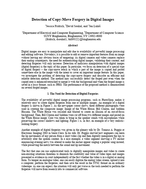
Detection of Copy-Move Forgery in Digital Imagesa Jessica Fridrich,b David Soukal, and a Jan Lukáša Department of Electrical and Computer Engineering,b Department of Computer ScienceSUNY Binghamton, Binghamton, NY 13902-6000{fridrich, dsoukal1, bk89322}@AbstractDigital images are easy to manipulate and edit due to availability of powerful image processing and editing software. Nowadays, it is possible to add or remove important features from an image without leaving any obvious traces of tampering. As digital cameras and video cameras replace their analog counterparts, the need for authenticating digital images, validating their content, and detecting forgeries will only increase. Detection of malicious manipulation with digital images (digital forgeries) is the topic of this paper. In particular, we focus on detection of a special type of digital forgery – the copy-move attack in which a part of the image is copied and pasted somewhere else in the image with the intent to cover an important image feature. In this paper, we investigate the problem of detecting the copy-move forgery and describe an efficient and reliable detection method. The method may successfully detect the forged part even when the copied area is enhanced/retouched to merge it with the background and when the forged image is saved in a lossy format, such as JPEG. The performance of the proposed method is demonstrated on several forged images.1. The Need for Detection of Digital ForgeriesThe availability of powerful digital image processing programs, such as PhotoShop, makes it relatively easy to create digital forgeries from one or multiple images. An example of a digital forgery is shown in Figure 1. As the newspaper cutout shows, three different photographs were used in creating the composite image: Image of the White House, Bill Clinton, and Saddam Hussein. The White House was rescaled and blurred to create an illusion of an out-of-focus background. Then, Bill Clinton and Saddam were cut off from two different images and pasted on the White House image. Care was taken to bring in the speaker stands with microphones while preserving the correct shadows and lighting. Figure 1 is, in fact, an example of a very realistic-looking forgery.Another example of digital forgeries was given in the plenary talk by Dr. Tomaso A. Poggio at Electronic Imaging 2003 in Santa Clara. In his talk, Dr. Poggio showed how engineers can learn the lip movements of any person from a short video clip and then digitally manipulate the lips to arbitrarily alter the spoken content. In a nice example, a video segment showing a TV anchor announcing evening news was altered to make the anchor appear singing a popular song instead, while preserving the match between the sound and lip movement.The fact that one can use sophisticated tools to digitally manipulate images and video to create non-existing situations threatens to diminish the credibility and value of video tapes and images presented as evidence in court independently of the fact whether the video is in a digital or analog form. To tamper an analogue video, one can easily digitize the analog video stream, upload it into a computer, perform the forgeries, and then save the result in the NTSC format on an ordinary videotape. As one can expect, the situation will only get worse as the tools needed to perform the forgeries will move from research labs to commercial software.Figure 1 Example of a digital forgery.Despite the fact that the need for detection of digital forgeries has been recognized by the research community, very few publications are currently available. Digital watermarks have been proposed as a means for fragile authentication, content authentication, detection of tampering, localization of changes, and recovery of original content [1]. While digital watermarks can provide useful information about the image integrity and its processing history, the watermark must be present in the image before the tampering occurs. This limits their application to controlled environments that include military systems or surveillance cameras. Unless all digital acquisition devices are equipped with a watermarking chip, it will be unlikely that a forgery-in-the-wild will be detectable using a watermark.It might be possible, but very difficult, to use unintentional camera “fingerprints” related to sensor noise, its color gamut, and/or its dynamic range to discover tampered areas in images. Another possibility for blind forgery detection is to classify textures that occur in natural images using statistical measures and find discrepancies in those statistics between different portions of the image ([2], [3]). At this point, however, it appears that such approaches will produce a large number of missed detections as well as false positives.In the next section, we introduce one common type of digital forgeries – the copy-move forgery – and show a few examples. Possible approaches to designing a detector are discussed in Section 3. In Section 4, we describe the detection method based on approximate block matching. Thisapproach proved to be by far the most reliable and efficient. The method is tested in the lastSection 5 on a few forgeries. In the same section, we summarize the paper and outline future research directions.2. Copy-Move ForgeryBecause of the extraordinary difficulty of the problem and its largely unexplored character, the authors believe that the research should start with categorizing forgeries by their mechanism, starting with the simple ones, and analyzing each forgery type separately. In doing so, one will build a diverse Forensic Tool Set (FTS). Even though each tool considered separately may not be reliable enough to provide sufficient evidence for a digital forgery, when the complete set of tools is used, a human expert can fuse the collective evidence and hopefully provide a decisive answer. In this paper, the first step towards building the FTS is taken by identifying one very common class of forgeries, the Copy-Move forgery, and developing efficient algorithms for its detection.In a Copy-Move forgery, a part of the image itself is copied and pasted into another part of the same image. This is usually performed with the intention to make an object “disappear” from the image by covering it with a segment copied from another part of the image. Textured areas, such as grass, foliage, gravel, or fabric with irregular patterns, are ideal for this purpose because the copied areas will likely blend with the background and the human eye cannot easily discern any suspicious artifacts. Because the copied parts come from the same image, its noise component, color palette, dynamic range, and most other important properties will be compatible with the rest of the image and thus will not be detectable using methods that look for incompatibilities in statistical measures in different parts of the image. To make the forgery even harder to detect, one can use the feathered crop or the retouch tool to further mask any traces of the copied-and-moved segments.Examples of the Copy-Move forgery are given in Figures 2–4. Figure 2 is an obvious forgery that was created solely for testing purposes. In Figure 3, you can see a less obvious forgery in which a truck was covered with a portion of the foliage left of the truck (compare the forged image with its original). It is still not too difficult to identify the forged area visually because the original and copied parts of the foliage bear a suspicious similarity. Figure 4 shows another Copy-Move forgery that is much harder to identify visually. This image has been sent to the authors by a third party who did not disclose the nature or extent of the forgery. We used this image as a real-life test for evaluating our detection tools. A visual inspection of the image did not reveal the presence of anything suspicious.Figure 2 Test image “Hats”.Figure 3 Forged test image “Jeep” (above) and its original version (below).Figure 4 Test image “Golf” with an unknown original.3. Detection of Copy-Move ForgeryAny Copy-Move forgery introduces a correlation between the original image segment and the pasted one. This correlation can be used as a basis for a successful detection of this type of forgery. Because the forgery will likely be saved in the lossy JPEG format and because of a possible use of the retouch tool or other localized image processing tools, the segments may not match exactly but only approximately. Thus, we can formulate the following requirements for the detection algorithm:1.The detection algorithm must allow for an approximate match of small image segments2.It must work in a reasonable time while introducing few false positives (i.e., detectingincorrect matching areas).3.Another natural assumption that should be accepted is that the forged segment will likelybe a connected component rather than a collection of very small patches or individual pixels.In this section, two algorithms for detection of the Copy-Move forgery are developed – one that uses an exact match for detection and one that is based on an approximate match.Before describing the best approach based on approximate block matching that produced the best balance between performance and complexity, two other approaches were investigated – Exhaustive search and Autocorrelation.3.1 Exhaustive searchThis is the simplest (in priciple) and most obvious approach. In this method, the image and its circularly shifted version (see Figure 5) are overlaid looking for closely matching image segments. Let us assume that x ij is the pixel value of a grayscale image of size M×N at the position i, j. In the exhaustive search, the following differences are examined:| x ij – x i+k mod(M) j+l mod(N) |, k = 0, 1, …, M–1, l = 0, 1, …, N–1 for all i and j.It is easy to see that comparing x ij with its cyclical shift [k,l] is the same as comparing x ij with its cyclical shift [k’,l’], where k’=M–k and l’=N–l.Thus, it suffices to inspect only those shifts [k,l] with 1≤k ≤M/2, 1≤l ≤N/2, thus cutting the computational complexity by a factor of 4.Figure 5 Test image “Lenna” and its circular shift.For each shift [k,l], the differences ∆x ij= | x ij – x i+k mod(M) j+lmod(N)|, are calculated andthresholded with a small threshold t . The threshold selection is problematic, because in natural images, a large amount of pixel pairs will produce differences below the threshold t . However, according to our requirements we are only interested in connected segments of certain minimal size. Thus, the thresholded difference ∆x ij is further processed using the morphological opening operation (see, for example [ImgProcBook]). The image is first eroded and then dilated with the neighborhood size corresponding to the minimal size of the copy-moved area (in experiments, the 10×10 neighborhood was used). The opening operation successfully removes isolated points.Although this simple exhaustive search approach is effective, it is also quite computationally expensive. In fact, the computational complexity of the exhaustive search makes it impractical for practical use even for medium-sized images. An estimate of the computational complexity of the algorithm is given below.During the detection, all possible shifts [k ,l ] with 1≤ k , l ≤ M /2 need to be inspected. For each shift, every pixel pair must be compared, thresholded, and then the whole image must be eroded and dilated. The comparison and image processing require the order of MN operations for one shift. Thus, the total computational requirements are proportional to (MN )2. For example, the computational requirements for an image that is twice as big are 16 times larger. This makes the exhaustive search a viable option only for small images.3.2 AutocorrelationThe autocorrelation of the image x of the size M ×N is defined by the formula:1 ..., ,0,,1 ..., ,0, ,11,,,−=−==∑∑==++N l j M k i x xr M i N j l j k i j i l k .The autocorrelation can be efficiently implemented using the Fourier transform utilizing the factthat r = x ∗xˆ, where ij x ˆ = x M +1–i ,N +1–j , i = 0, …, M –1, j = 0, …, N –1. Thus we have r = F –1{F (x ) F (xˆ)}, where F denotes the Fourier transform.The logic behind the detection based on autocorrelation is that the original and copied segments will introduce peaks in the autocorrelation for the shifts that correspond to the copied-moved segments. However, because natural images contain most of their power in low-frequencies, if the autocorrelation r is computed directly for the image itself, r would have very large peaks at the image corners and their neighborhoods. Thus, we compute the autocorrelation not from the image directly, but from its high-pass filtered version.Several high-pass filters were tested: Marr edge detector, Laplacian edge detector, Sobel edge detector, and noise extracted using the 3×3 Wiener filter (see, for example, [ImgProcBook]). The best performance was obtained using the 3×3 Marr filter.Assuming the minimal size of a copied-moved segment is B , the autocorrelation copy-move detection method consists of the following steps:1. Apply the Marr high-pass filter to the tested image.2. Compute the autocorrelation r of the filtered image.3. Remove half of the autocorrelation (Autocorrelation is symmetric.).4. Set r = 0 in the neighborhood of two remaining corners of the entire autocorrelation.5. Find the maximum of r , identify the shift vector, and examine the shift using the exhaustivemethod (this is now computationally efficient because we do not have to perform theexhaustive search for many different shift vectors).6.If the detected area is larger than B, finish, else repeat Step 5 with the next maximum of r. Although, this method is simple and does not have a large computational complexity, it often fails to detect the forgery unless the size of the forged area is at least ¼ of linear image dimensions (according to our experiments).Both the exhaustive search and the autocorrelation method were abandoned in favor of the third approach that worked significantly better and faster than previous approaches.4. Detection of Copy-Move Forgery by Block Matching4.1 Exact matchThe first algorithm described in this section is for identifying those segments in the image that match exactly. Even though the applicability of this tool is limited, it may still be useful for forensic analysis. It also forms the basis of the robust match detailed in the next section.In the beginning, the user specifies the minimal size of the segment that should be considered for match. Let us suppose that this segment is a square with B×B pixels. The square is slid by one pixel along the image from the upper left corner right and down to the lower right corner. For each position of the B×B block, the pixel values from the block are extracted by columns into a row of a two-dimensional array A with B2 columns and (M–B+1)(N–B+1) rows. Each row corresponds to one position of the sliding block.Two identical rows in the matrix A correspond to two identical B×B blocks. To identify the identical rows, the rows of the matrix A are lexicographically ordered (as B×B integer tuples). This can be done in MN log2(MN) steps. The matching rows are easily searched by going through all MN rows of the ordered matrix A and looking for two consecutive rows that are identical.Figure 6 Results of the Block Match Copy-Detection forgery algorithm(the exact match mode with block size B=4).The matching blocks found in the BMP image of Jeep (Figure 3) for B=8 are shown in Figure 6. The blocks form an irregular pattern that closely matches the copied-and-moved foliage. The fact that the blocks form several disconnected pieces instead of one connected segment indicates that the person who did the forgery has probably used a retouch tool on the pasted segment to cover the traces of the forgery. Note that if the forged image had been saved as JPEG, vast majority ofidentical blocks would have disappeared because the match would become only approximate and not exact (compare the detection results with the robust match in Figure 8). This also why the exact match analysis of images from Figures 2 and 4 did not show any exactly matching blocks. In the next section, the algorithm for the robust match is given and its performance evaluated.4.2 Robust matchThe idea for the robust match detection is similar to the exact match except we do not order and match the pixel representation of the blocks but their robust representation that consists of quantized DCT coefficients. The quantization steps are calculated from a user-specified parameter Q. This parameter is equivalent to the quality factor in JPEG compression, i.e., the Q-factor determines the quantization steps for DCT transform coefficients. Because higher values of the Q-factor lead to finer quantization, the blocks must match more closely in order to be identified as similar. Lower values of the Q-factor produce more matching blocks, possibly some false matches.The detection begins in the same way as in the exact match case. The image is scanned from the upper left corner to the lower right corner while sliding a B×B block. For each block, the DCT transform is calculated, the DCT coefficients are quantized and stored as one row in the matrix A. The matrix will have (M– B+1)(N–B+1) rows and B×B columns as for the exact match case.The rows of A are lexicographically sorted as before. The remainder of the procedure, however, is different. Because quantized values of DCT coefficients for each block are now being compared instead of the pixel representation, the algorithm might find too many matching blocks (false matches). Thus, the algorithm also looks at the mutual positions of each matching block pair and outputs a specific block pair only if there are many other matching pairs in the same mutual position (they have the same shift vector). Towards this goal, if two consecutive rows of the sorted matrix A are found, the algorithm stores the positions of the matching blocks in a separate list (for example, the coordinates of the upper left pixel of a block can be taken as its position) and increments a shift-vector counter C. Formally, let (i1, i2) and (j1, j2) be the positions of the two matching blocks. The shift vector s between the two matching blocks is calculated ass = (s1, s2) = (i1 – j1, i2 – j2).Because the shift vectors –s and s correspond to the same shift, the shift vectors s are normalized, if necessary, by multiplying by –1 so that s1 ≥ 0. For each matching pair of blocks, we increment the normalized shift vector counter C by one:C(s1, s2) = C(s1 , s2) + 1 .The shift vectors are calculated and the counter C incremented for each pair of consecutive matching rows in the sorted matrix A. The shift vector C is initialized to zero before the algorithm starts. At the end of the matching process, the counter C indicates the frequencies with which different normalized shift vectors occur. Then the algorithm finds all normalized shift vectors s(1), s(2), …, s(K), whose occurrence exceeds a user-specified threshold T: C(s(r)) > T for all r = 1, …, K. For all normalized shift vectors, the matching blocks that contributed to that specific shift vector are colored with the same color and thus identified as segments that might have been copied and moved.The value of the threshold T is related to the size of the smallest segment that can be identified by the algorithm. Larger values may cause the algorithm to miss some not-so-closely matchingblocks, while too small a value of T may introduce too many false matches. We repeat that the Q-factor controls the sensitivity of the algorithm to the degree of matching between blocks, while the block size B and threshold T control the minimal size of the segment that can be detected.For the robust match, we have decided to use a larger block size, B =16, to prevent too many false matches (larger blocks have larger variability in DCT coefficients). However, this larger block size means that a 16×16 quantization matrix must be used instead of simply using the standard quantization matrix of JPEG. We have found out from experiments that all AC DCT coefficients for 16×16 blocks are on average 2.5 times larger than for 8×8 blocks and the DC term is twice as big. Thus, the quantization matrix (for the Q-factor Q ) that is used for quantizing the DCT coefficients in each 16×16 block has the following form= =88828128222118120088881188165.2...5.25.2............5.2...5.25.25.2...5.22' where ,5.25.25.2'q q q q q q q q q Q I q I q I q Q Qand q ij is the standard JPEG quantization matrix with quality factor Q and I is an 8×8 unit matrix (all elements equal to 1). We acknowledge that this form is rather ad hoc, but because the matrix gave very good performance in practical tests and because small changes to the matrix influence the results very little, we did not investigate the selection of the quantization matrix further.Note regarding color images: In both Exact and Robust Match, if the analyzed image is a color image, it is first converted to a grayscale image using the standard formula I = 0.299 R + 0.587 G + 0.114 B , before proceeding with further analysis.5. Robust Match PerformanceWe have implemented the detection algorithm in C and tested on all three forged images. The output from the detection algorithm are two images. In the first image, the matching blocks are all colored with the same tint. In Figure 7 below, a yellow tint was used for rendering the copied-moved segments. The second output image shows the copied-moved blocks on a black background. Different colors correspond to different shift vectors. Note that the algorithm likely falsely identified two matching segments in the sky. It is to be expected that flat, uniform areas, such as the sky, may lead to false matches. Human interpretation is obviously necessary to interpret the output of any Copy-Move detection algorithm.Figure 7 shows the output of our detection routine applied to Figure 4. Although visual inspection did not reveal any suspicious artifacts, the algorithm identified several three large segments in the grass that were copied and pasted perhaps to cover up some object on the grass. Knowing the program output, we were able to visually confirm a suspicious match in the otherwise “random looking” grass texture.Figure 8 shows the result of robust match for “Hats” (Figure 2). Because the elliptic area on the orange hat has been copied to two other locations, three different shift vectors have been correctly found by the program (green, blue, and red colors). Note that the red color is almost completely covered by the green color (upper right ellipse) and the blue ellipse (bottom right). One green ellipse is covered by the blue ellipse in the center of the image. The fourth color, yellow, identifies the second copied and moved square segment.The result of the robust match for the “Jeep” image (Figure 3) is shown in Figure 9. The copied-moved foliage is captured much more accurately than for the exact match (c.f., Figure 6).AcknowledgementsThe work on this paper was supported by Air Force Research Laboratory, Air Force Material Command, USAF, under a research grant number F30602-02-2-0093. The U.S. Government is authorized to reproduce and distribute reprints for Governmental purposes notwithstanding any copyright notation there on. The views and conclusions contained herein are those of the authors and should not be interpreted as necessarily representing the official policies, either expressed or implied, of Air Force Research Laboratory, or the U. S. Government.Figure 7Figure 8 Figure 9References[1]J. Fridrich, “Methods for "Methods for Tamper Detection in Digital Images", Proc. ACMWorkshop on Multimedia and Security, Orlando, FL, October 30−31, 1999, pp. 19−23. [2]S. Saic, J. Flusser, B. Zitová, and J. Lukáš, “Methods for Detection of AdditionalManipulations with Digital Images”, Research Report, Project RN199******** "Detection of Deliberate Changes in Digital Images", ÚTIA AV ČR, Prague, December 1999 (partially in Czech).[3]J. Lukáš, “Digital Image Authentication“, Workshop of Czech Technical University 2001,Prague, Czech Republic, February 2001.[4]Img. Processing book。
detectmultiscale函数参数含义

detectmultiscale函数参数含义detectMultiscale函数是OpenCV中的一个用于目标检测的函数。
它的作用是在图像中检测出具有不同尺寸的目标,并返回这些目标的位置信息。
这个函数包含多个参数,下面我将逐一介绍这些参数的含义。
1. imageimage是待检测的输入图像,它可以是一个灰度图像或彩色图像。
2. objectsobjects是输出参数,表示检测到的目标位置信息。
它是一个vector,每个元素都是一个Rect类型的矩形,表示检测到的目标在原始图像中的位置和大小。
3. scaleFactorscaleFactor是表示图像缩放比例的参数,它是一个浮点数,表示每次缩小图像的比例。
例如,如果scaleFactor=1.1,则每次缩小图像的比例为10%。
4. minNeighborsminNeighbors是表示目标候选框之间最小距离的参数,它是一个整数。
该参数用于过滤掉一些误检目标,减少误检率。
具体来说,如果minNeighbors=3,则检测到的目标矩形之间的重叠部分的像素数量必须大于等于3,才能被认为是真正的目标。
5. flagsflags是一个可选的参数,它用于指定检测方式。
目前支持两种方式:CASCADE_DO_CANNY_PRUNING和CASCADE_SCALE_IMAGE。
6. minSizeminSize是一个可选的参数,它表示目标最小尺寸。
如果目标的实际尺寸小于minSize,则会被忽略。
7. maxSizemaxSize是一个可选的参数,它表示目标最大尺寸。
如果目标的实际尺寸大于maxSize,则会被忽略。
需要注意的是,这些参数的取值会影响检测结果,因此需要根据具体的应用场景进行调整。
UnexplodedOrdnanceDetectionandMitigation
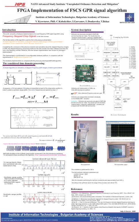
Mitigation”FPGA algorithmTwo narrow-band chirps ()each with central frequency and bandwidth ()are combined to form one chirp with bandwidth ()M=2f B=Δf 2B m NATO ASI UXO 2008The correlation is performed for 108ìs Resultsf fA sequence of narrowband pulses is transmitted at each of the observation position in order to obtain a synthetic range profile.The frequencies are spaced by step M LFM centerB MV2The range resolution is:A part of the transmitted wave form in the time domain /Matlab simulation/:MATLAB simulation of the synthetic range profile constructed in the time domain by combining14narrowband chirps according to this algorithm.:A four-layered ground environment is simulated 14narrow-band chirps are combined into one wide-band chirpSynthetic range profile in dBSynthetic range profile that includes envelopes of 3echo signalsreflected from layers 2,3and 4The receiver block diagramThe used platform[]The total synthesis estimation parameters are:number of slices =8937BRAM =30Mult18x18=62After the simulation performing the real time constraints were approximately found 400ìs According to the synthesis report,the usage of the processor was almost 75%.Sample issue of a correlation on the ModelsimsimulatorТМThe experimentThe transmitter outputReferences[1]Behar V.,Chr.Kabakchiev,“,Proc.IRS-07,4-9Sept.,2007,Cologne,pp.635-639“Stepped-Frequency Processing in Low-Frequency GPR [2]Daniels D,Ground penetrating radar,2nd edition,The Institution of Electrical Engineers,London,200[]3Mikhnev V.,Microwave reconstruction approach for stepped-frequency radar,15th World Conf.on Non-Destructive Testing,15-21Oct,Rome,2000.[4]Nel W.,J.Tait,R.Lord and A.Wilkinson,"The use of a frequency domain stepped frequency technique to obtain high range resolution on the CSIR X-Band SAR system,"Proc.6th IEEE AFRICON Conf.,AFRICON'02,George,South Africa,vol.1,2002,327-332.[5]Zhang Q.,Jin Y .,Aspects of radar imaging using frequency-stepped chirp signals,EURASIP Journal on Applied Signal processing,vol.2006,1-8.All blocks are implemented on VHDL via Xilinx ISE development platformXilinx cores are usedIntlectual Properies All blocks are implemented and tested individuallyon the MODELSIM simulatorТМVerification -All blocks are previously simulated in MATLAB and test benches are made.The results from the hardwareimplementation,obtained in MODELSIM ,simulator are compared with the MATLAB test benches.ТМf0,m 0,m+1=f +ff0,min1=fm=1,...,MδD=∆ f∆。
balluff bni iol-709-000-k006 bni iol-710-000-k006

BNI IOL-709-000-K006 BNI IOL-710-000-K006IO-Link Sensor-Hub analogUser’s GuideContent1Notes to the user 21.1Structure of the guide 21.2Typographical conventions 2Enumerations 2 Actions 2 Syntax 2 Cross-references 21.3Symbols 21.4Abbreviations 21.5Divergent views 2 2Safety 32.1Intended use 32.2Installation and startup 32.3General safety Notes 32.4Resistance to Aggressive Substances 3Hazardous voltage 3 3Getting Started 43.1Connection overview 43.2Mechanical connection 53.3Electrical connection 53.4Function ground 53.5IO-Link connection 53.6Digital Sensors 63.7Analogue Sensors 6 4IO-Link Interface 74.1IO-Link Data 74.2Process data inputs 74.3Process data outputs 84.4Parameter data/ On-request data 8Identification data 8 Inversion 9 Switch point enable 9 Switch point 94.5Errors 104.6Events 10 5Technical Data 115.1Dimensions 115.2Mechanical data 115.3Electrical data 115.4Operating conditions 115.5Function indicators 12Module LEDs 12 Digital Input LEDs 12 Analogue Input LEDs 12 6Appendix 136.1Type designation code 136.2Order information 13IO-Link Sensor-HubBNI IOL-709-… / BNI IOL-710-…1 Notes to the user1.1 Structure of theguide The Guide is organized so that the sections build on one another. Section 2 : Basic safety information. …………1.2 Typographicalconventions The following typographical conventions are used in this Guide. EnumerationsEnumerations are shown in list form with bullet points.• Entry 1, • Entry 2.Actions Action instructions are indicated by a preceding triangle. The result of an action is indicated by an arrow.Action instruction 1. Action result.Action instruction 2. SyntaxNumbers:Decimal numbers are shown without additional indicators (e.g. 123),Hexadecimal numbers are shown with the additional indicator hex (e.g. 00hex ).Cross-references Cross-references indicate where additional information on the topic can be found.1.3 SymbolsAttention!This symbol indicates a security notice which most be observed.NoteThis symbol indicates general notes.1.4 AbbreviationsBCD BNI CV DPP I-Port EMC FE IOL LSB MSB SP SPDU VVBinary coded switch Balluff Network InterfaceCurrent Version: BNI IOL 709… Direct Parameter Page Digital input portElectromagnetic Compatibility Function ground IO-LinkLeast Significant Bit Most Significant Bit Switch PointService Protocol Data UnitVoltage version: BNI IOL 710…1.5 Divergent views Product views and images can differ from the specified product in this manual. They serve only as an illustration.2 Safety2.1 Intended use The BNI IOL-… is a decentralized sensor input module which is connected to a host IO-Linkmaster over an IO-Link interface.2.2 Installation andstartup Attention!Installation and startup are to be performed by trained technical personnel only. Skilled specialists are people who are familiar with the work such as installation and the operation of the product and have the necessary qualifications for these tasks. Any damage resulting from unauthorized tampering or improper use shall void warranty and liability claims against the manufacturer. The operator is responsible for ensuring that the valid safety and accident prevention regulations are observed in specific individual cases.2.3 General safetyNotes Commissioning and inspectionBefore commissioning, carefully read the User's Guide.The system must not be used in applications in which the safety of persons depends on the function of the device.Intended useWarranty and liability claims against the manufacturer shall be rendered void by damage from:•Unauthorized tampering•Improper use•Use, installation or handling contrary to the instructions provided in this User's Guide.Obligations of the owner/operator!The device is a piece of equipment in accordance with EMC Class A. This device can produce RF noise. The owner/operator must take appropriate precautionary measures against this for its use. The device may be used only with a power supply approved for this. Only approved cables may be connected.MalfunctionsIn the event of defects and device malfunctions that cannot be rectified, the device must be taken out of operation and protected against unauthorized use.Approved use is ensured only when the housing is fully installed.2.4 Resistance toAggressiveSubstances Attention!The BNI modules always have good chemical and oil resistance. When used in aggressive media (such as chemicals, oils, lubricants and coolants, each in a high concentration (i.e. too little water content)), the material must first be checked for resistance in the particular application. No defect claims may be asserted in the event of a failure or damage to the BNI modules caused by such aggressive media..Hazardous voltage Attention!Disconnect all power before servicing equipment.NoteIn the interest of continuous improvement of the product,Balluff GmbH reserves the right to change the technical data of the product and the content of these instructions at any time without notice.IO-Link Sensor-HubBNI IOL-709-… / BNI IOL-710-…3 Getting Started3.1 Connectionoverview1 Mounting hole2 IO-Link interface3 Analogue input-Port 14 Status-LED: Analogue port5 Analogue input port 36 Status-LED: digital input Pin 27 Digital input port 18 Status-LED: Digital port Pin 49 Digital input port 3 10 Status LED “Power Supply”11 Digital input port 212 Digital input port 013 Analogue input port 214 Analogue input port 015 Label16 Status-LED …COM“17 Function ground connection3 Getting Started3.2 Mechanicalconnection The BNI IOL modules are attached using 3 M4 screws (Item 1, Fig. 3-1/3-2).3.3 Electricalconnection The Sensor Hub modules require no separate supply voltage connection. Power is provided through the IO-Link interface by the host IO-Link Master.3.4 Function groundThe modules are provided with a ground terminal.Connect Sensor Hub module to the ground terminal.NoteThe FE connection from the housing to the machine must be low-impedance and as short as possible.3.5 IO-LinkconnectionThe IO-Link connection is made using an M12 connector (A-coded, male).IO-Link (M12, A-coded, male)Pin Function 1Supply voltage, +24 V, max. 1.6 A 2 - 3 GND, reference potential4 C/Q, IO-Link data transmission channelConnection protection ground to FE terminal, if present. Connect the incoming IO-Link line to the Sensor Hub.NoteA standard sensor cable is used for connecting to the host IO-Link Master.IO-Link Sensor-HubBNI IOL-709-… / BNI IOL-710-…3 Getting Started3.6 Digital Sensors Digital input port (M12, A-coded, female)Pin Function 1 +24 V, 100 mA 2 Standard Input 3 0 V, GND 4 Standard Input 5 -NoteFor the digital sensor inputs follow the input guideline per EN 61131-2, Type 2.3.7 AnalogueSensors Analogue input port (M12, A-coded, female)Pin Function1 +24 V, 100 mA2BNI IOL-709...: 4 - 20 mABNI IOL-710…:n.c. 3 0 V, GND4BNI IOL-710...: 0 - 10 V BNI IOL-709…:n.c 5 FE, function groundNoteUnused I/O port sockets must be fitted with cover caps to ensure IP67 protection rating.NoteOvercurrent (> 25mA) on the BNI IOL-709 Module´s inputs can distort the measurement results of the other channels and it may leads to malfunction..4 IO-Link Interface4.1 IO-Link Data Baudrate COM2 (38,4 kBaud)Frame type 1Minimum cycle time 3 msProcess data cycle 30 ms with minimum cycle time4.2 Process datainputs BNI IOL-710-…/BNI IOL-709-…(Sensor-Hub digital/analog)Process data length 10Byte:Byte 0 Byte 17 6 5 4 3 2 1 0 7 6 5 4 3 2 1 0InputPort7Pin4InputPort6Pin4InputPort5Pin4InputPort4Pin4SwitchPoint1Port3SwitchPoint1Port2SwitchPoint1Port1SwitchPoint1PortInputPort7.Pin2InputPort6.Pin2InputPort5.Pin2InputPort4.Pin2SwitchPoint2Port3SwitchPoint2Port2SwitchPoint2Port1SwitchPoint2PortByte 2 Byte 37 6 5 4 3 2 1 0 7 6 5 4 3 2 1 0Error1Error2Error3MSBAnalogue valueLSBPort 0Byte 4 Byte 57 6 5 4 3 2 1 0 7 6 5 4 3 2 1 0Error1Error2Error3MSBAnalogue valueLSBPort 1Byte 6 Byte 77 6 5 4 3 2 1 0 7 6 5 4 3 2 1 0Error1Error2Error3MSBAnalogue valueLSBPort 2Byte 8 Byte 97 6 5 4 3 2 1 0 7 6 5 4 3 2 1 0Error1Error2Error3MSBAnalogue valueLSBPort 3IO-Link Sensor-HubBNI IOL-709-… / BNI IOL-710-…4 IO-Link InterfaceInput: Input-Signal at Port and PinSwitch Point: The switch point bits show a switch pointoverrun. The switch point can be configuredby parameter ( see 0.0 - “Switch pointenable” and 0.0 - “Switch point”)Analogue value: VV: actual voltage value between0 and 1056 (1Bit = 0.01V)CV: actual current value between0 and 2150 (1Bit = 0.01mA)Error:• Error 1 • Error 2 • Error 3 Overcurrent/short circuit on sensor supply Measurement range overflow Measurement range undercut (only CV)4.3 Process dataoutputsThere are no outputs at BNI IOL-710-... and BNI IOL-709-... modules.4.4 Parameter data/On-request dataDPP SPDU Parameter DatawidthAccess Index Index Sub-indexIdentificationData07hex Vendor ID 2 ByteReadonly 08hex09hex Device ID 3 Byte0A hex0B hex10hex0 Vendor Name 8 Byte11hex0 Vendor text 16 Byte12hex0 Product Name 34 Byte13hex0 Product ID 21 Byte14hex0 Product text 34 Byte16hex Hardware Revision 3 Byte17hex0 Firmware Revision 3 ByteIdentification data Type Device ID VersionBNI IOL-710-000-K006 050201hex Voltage versionBNI IOL-709-000-K006 050202hex Current version4 IO-Link InterfaceDPPSPDUParameter Data width Value rangeDefault- valueIndex Index Sub-index P a r a m e t e r D a t a10hex 40hex640 1-16 Inversion 2 Byte 0000hex …FFFF hex 0000hex 11hex 12hex 41hex650 1-8 Switch point enable 1 Byte 00hex …FF hex 00hex 42hex660 Switch point 1 Port 0 2 Byte 0000hex … 03E8hex 0000hex 43hex670 Switch point 1 Port 1 2 Byte 0000hex … 03E8hex 0000hex 44hex680 Switch point 1 Port 2 2 Byte 0000hex … 03E8hex 0000hex 45hex690 Switch point 1 Port 3 2 Byte 0000hex … 03E8hex 0000hex 46hex700 Switch point 2 Port 0 2 Byte 0000hex … 03E8hex 0000hex 47hex710 Switch point 2 Port 1 2 Byte 0000hex … 03E8hex 0000hex 48hex720 Switch point 2 Port 2 2 Byte 0000hex … 03E8hex 0000hex 49hex73Switch point 2 Port 32 Byte0000hex … 03E8hex0000hexInversionInversion of the input signals:Byte 0Byte 176543217654321I n v e r s i o n P o r t 7 P i n 4I n v e r s i o n P o r t 6 P i n 4I n v e r s i o n P o r t 5 P i n 4I n v e r s i o n P o r t 4 P i n 4I n v e r s i o n S P 1 P o r t 3I n v e r s i o n S P 1 P o r t 2I n v e r s i o n S P 1 P o r t 1I n v e r s i o n S P 1 P o r t 0I n v e r s i o n P o r t 7 P i n 2I n v e r s i o n P o r t 6 P i n 2I n v e r s i o n P o r t 5 P i n 2I n v e r s i o n P o r t 4 P i n 2I n v e r s i o n S P 2 P o r t 3I n v e r s i o n S P 2 P o r t 2I n v e r s i o n S P 2 P o r t 1I n v e r s i o n S P 2 P o r t 0Switch point enableEnable the switch points by setting the enable bitsByte 07654321E n a b l e s w i t c h p o i n t 2 P o r t 3E n a b l e s w i t c h p o i n t 2 P o r t 2E n a b l e s w i t c h p o i n t 2 P o r t 1E n a b l e s w i t c h p o i n t 2 P o r t 0E n a b l e s w i t c h p o i n t 1 P o r t 3E n a b l e s w i t c h p o i n t 1 P o r t 2E n a b l e s w i t c h p o i n t 1 P o r t 1E n a b l e s w i t c h p o i n t 1 P o r t 0Switch pointByte 0Byte 1 7 6 5 4 3217654321Switch pointValue range (dec) CV= 400...2000 VV= 0 (1000)BNI IOL-709-… / BNI IOL-710-…4 IO-Link Interface4.5 Errors Byte 0Byte 1Device application error: 80hex11hex Index not available 12hex Subindex not available 30hex Value out of range4.6 EventsClass/QualifierCode (high + low)Mode Type InstanceP a r a m e t e r D a t aappears Error AL Device Hardware supply Supply low voltage U2 = supply + 24VC0hex 30hex 03hex 5000hex 0100hex 0010hex 0002hex F3hex5112hex disappears ErrorAL Device Hardware supply Supply low voltage U2 = supply + 24V80hex 30hex 03hex 5000hex 0100hex 0010hex 0002hexB3hex 5112hexappears Error AL Device Hardware supply supply peripheryC0hex30hex 03hex 5000hex 0100hex0060hexF3hex 5160hexdisappears ErrorAL Device Hardware supply supply periphery80hex30hex 03hex5000hex0100hex0060hexB3hex5160hex5 Technical Data5.1 Dimensions5.2 Mechanical data Housing Material Plastic, transparentIO-Link-Port M12, A-coded, maleInput-Ports 8x M12, A-coded, femaleEnclosure rating IP67 (only when plugged-in and threaded-in)Weight 90 gDimensions(L × W × H, excluding connector)115 × 50 × 30,8 mm5.3 Electrical data Operating voltage 18 ... 30,2 V DC, per EN 61131-2Ripple < 1 %Current draw without load ≤ 40 mA5.4 Operatingconditions Operating temperature -5 °C … +55 °C Storage temperature -25 °C … +70 °CBNI IOL-709-… / BNI IOL-710-…5 Technical Data5.5 FunctionindicatorsModule LEDs LED 5, IO-Link CommunicationStatus FunctionGreen No CommunicationGreen negative pulsed Communication OKRed Communication line overloadOff Module unpoweredLED 4, Power supply statusStatus FunctionGreen Module power is OKGreen slowly flashing Short circuitGreen rapidly flashing Module power supply < 18 VOff Module unpowered Digital Input LEDs LED 3, Input Pin 4 and LED 2, Input Pin 2Status FunctionYellow Input signal = 1Off Input signal = 0Analogue Input LEDs LED 1, Analogue input portStatus Signal 709 (4-20 mA) Signal 710 (0-10 V) Green ≥ 4 mA - ≤ 20 mA> 0,05 VRed < 4 mA - > 20 mA > 10,05 V6 Appendix6.1 Type designationcode6.2 OrderinformationType Order CodeBNI IOL-709-000-K006 BNI0007BNI IOL-710-000-K006 BNI0008BNI IOL-7xx-000-K006 Balluff Network InterfaceIO-Link interfaceFunctions710 = 8 digital inputs 0,15 A + 4 analog inputs 0 - 10 V709 = 8 digital inputs 0,15 A + 4 analog inputs 4 - 20 mAVariant000 = StandardvarianteMechanical configurationK006 =Plastic housing,Connectors:- BUS and Power supply: 1x M12x1, external thread- Input ports: 8x M12x1, internal threadBNI IOL-709-… / BNI IOL-710-… NotesBalluff GmbHSchurwaldstrasse 973765 Neuhausen a.d.F. GermanyTel. +49 7158 173-0 N r . 910442-726 E •01.125277 • E d i t i o n K 17 • R e p l a c e s E d i t i o n 1311 • S u b j e c t t o m o d i f i c a t i o n。
from mydetection import detection用法
from mydetection import detection用法From mydetection import detection用法介绍:from mydetection import detection是一种Python模块的导入方式,它可以用于导入一个名为detection的模块,并使其成为当前程序中可用的对象。
这个模块通常被用于图像处理和计算机视觉领域,它提供了一系列函数和类,可以用于目标检测、物体识别、人脸识别等任务。
使用方法:1. 导入模块要使用from mydetection import detection,首先需要将mydetection模块所在的路径添加到Python解释器的搜索路径中。
可以通过以下代码实现:import syssys.path.append('mydetection_path')其中mydetection_path是mydetection模块所在的路径。
然后,在你的Python代码中,可以通过以下方式导入mydetection 模块:from mydetection import detection2. 目标检测目标检测是计算机视觉领域中最基础、最重要的任务之一。
在mydetection模块中,提供了一个名为detect_object()的函数,可以用于目标检测。
该函数接受两个参数:输入图像和输出图像。
具体使用方法如下:import cv2from mydetection import detection# 读取图像img = cv2.imread('test.jpg')# 目标检测output_img = detect_object(img)# 显示结果cv2.imshow('output', output_img)cv2.waitKey(0)3. 物体识别物体识别是目标检测的进一步发展,它不仅可以检测出物体的位置,还可以对物体进行分类。
detectmultiscale 参数

detectMultiscale参数介绍在计算机视觉领域,目标检测是一个重要的任务。
它涉及到在图像或视频中定位和识别特定目标的过程。
OpenCV是一个流行的计算机视觉库,提供了许多用于目标检测的函数和算法。
其中之一是detectMultiscale函数,它可以用于在图像中检测多个尺度的目标。
detectMultiscale函数使用了级联分类器(Cascade Classifier)的方法来进行目标检测。
级联分类器是一种基于机器学习的方法,通过训练一个分类器来判断图像中是否存在特定目标。
它将图像分成不同大小的窗口,并对每个窗口应用分类器来判断是否包含目标。
参数说明detectMultiscale函数有几个参数可以调整,以便更好地适应不同的场景和需求。
image这是输入图像,可以是灰度图像或彩色图像。
通常情况下,灰度图像会比彩色图像更快地进行处理。
objects这是一个表示目标区域的矩形向量列表。
每个矩形包含了检测到的目标区域的位置和大小信息。
scaleFactor这个参数控制了每次缩放图像的比例。
默认值为1.1,表示每次缩放图像的尺寸增加10%。
较小的值会导致更多的计算量,但可能会错过一些小目标。
较大的值会减少计算量,但可能会导致一些目标被错过。
minNeighbors这个参数控制了每个候选目标必须在多少个邻近窗口中被检测到才能被认为是一个真正的目标。
默认值为3,较大的值会过滤掉一些误检测,但也可能会导致一些真正的目标被漏检。
flags这个参数控制了级联分类器的行为。
可以使用不同的标志来调整分类器对图像进行检测时的行为。
•CASCADE_SCALE_IMAGE:默认值,表示对图像进行缩放以适应不同尺度。
•CASCADE_FIND_BIGGEST_OBJECT:只返回最大的目标。
•CASCADE_DO_ROUGH_SEARCH:使用快速检测模式。
minSize这个参数指定了要检测的目标区域的最小尺寸。
探测限标准

探测限标准
探测限标准(Detection Limit Standard)是指在化学分析、环境监测、生物检测等领域中,用于确定某种物质或元素在样品中可被可靠检测到的最低浓度或最小量的标准。
这一标准对于保证分析结果的准确性和可靠性至关重要,因为它定义了分析方法能够区分样品中实际存在的目标物质与背景噪声之间的界限。
探测限的确定通常涉及以下步骤:
1. 样品准备:按照特定的实验设计准备样品,确保样品代表性和测试条件的一致性。
2. 重复测量:对含有已知低浓度目标物质的样品进行多次测量,以获得一系列数据。
3. 数据分析:利用统计学方法处理测量数据,计算出平均值和标准偏差。
4. 信噪比:根据国际纯粹与应用化学联合会 (IUPAC)的定义,探测限通常是信号与噪声比(S/N)为3:1时的浓度,即当信号值是噪声标准偏差的三倍时,认为该浓度为目标物质的探测限。
5. 验证:通过进一步的实验,如使用不同浓度的标准溶液进行验证,确保探测限的准确性和重复性。
探测限标准的设定对于环境法规的执行、食品安全的保障以及科学研究的数据解释等方面都有重要意义。
例如,在环境监测中,探测限可以帮助确定污染物是否低于法规规定的安全水平;在药物分析中,探测限可以确保药物成分的准确测定,从而保障药品质量和疗效。
因此,探测限标准的制定需要遵循严格的科学原则和方法,以确保其科学性和适用性。
芯片精灵检测

芯片精灵检测芯片精灵检测是一种通过图像处理和深度学习算法对芯片表面进行检测的技术。
通过检测芯片表面的缺陷和污染,可以有效提高芯片的质量和可靠性。
首先,芯片精灵检测需要获取芯片表面的图像。
可以使用显微镜对芯片进行放大拍摄,或者使用高分辨率摄像头对芯片进行拍摄。
得到的图像包含了芯片表面的纹理和特征。
然后,芯片精灵检测使用图像处理算法对芯片图像进行预处理。
这一步骤主要包括灰度化、滤波、边缘检测等操作,目的是减少图像的噪声和干扰,突出芯片表面的特征。
接下来,芯片精灵检测使用深度学习算法对预处理后的图像进行特征提取和分类。
深度学习算法可以通过训练大量的样本数据来学习芯片表面的正常和异常特征。
通过比对样本数据,可以将芯片表面的缺陷和污染与正常特征进行区分。
最后,芯片精灵检测根据深度学习算法的分类结果,给出对芯片表面的判断和评估。
如果芯片表面存在缺陷和污染,会发出报警信号,通知操作员进行相应的处理和修复。
如果芯片表面没有异常,将会给出正常的检测结果。
芯片精灵检测具有以下特点和优势:1. 高效准确:芯片精灵检测使用图像处理和深度学习算法,可以快速准确地对芯片表面进行检测。
相比传统的人工检测方法,大大提高了检测效率和准确度。
2. 自动化操作:芯片精灵检测可以实现自动化操作,不需要人力干预,大大减少了人工检测的成本和工作量。
3. 高灵敏度:芯片精灵检测可以检测到微小的缺陷和污染。
即使是表面上看不到的细微问题,也可以通过芯片精灵检测进行检测和判断。
4. 可扩展性:芯片精灵检测可以随着技术的进步和需求的变化而进行升级和扩展。
可以根据需要添加新的算法和功能,满足不同芯片的检测需求。
综上所述,芯片精灵检测是一种通过图像处理和深度学习算法对芯片表面进行检测的技术。
它可以提高芯片的质量和可靠性,实现自动化操作,提高检测效率和准确度。
在芯片制造和质量控制领域具有重要的应用价值。
目标检测代码

目标检测代码目标检测是计算机视觉领域的一项重要任务,其目标是在图像或视频中识别和定位特定的物体。
目标检测代码通常涉及多个步骤,包括图像预处理、模型训练和推断。
图像预处理是目标检测的第一步,它旨在将输入图像转换为适合模型输入的形式。
常见的预处理操作包括图像缩放、裁剪、归一化和增强等。
模型训练是目标检测的核心步骤,其目标是从标注的训练数据中学习目标的特征和表示。
常用的目标检测模型包括基于深度学习的物体检测模型,如Faster R-CNN、YOLO和SSD等。
模型训练涉及选择合适的模型结构、优化损失函数和调整模型超参数等。
模型推断是目标检测的最后一步,其目标是将模型应用于新的图像或视频数据中,实现目标检测的任务。
推断过程涉及将输入图像传递给训练好的模型,并通过模型输出来定位和识别图像中的目标。
在推断过程中,还需要使用一些后处理技术,如非极大值抑制(NMS)来去除重叠的检测框。
以下是一个简单的目标检测代码示例,以Faster R-CNN模型为例:1. 导入必要的库和模块import torchimport torchvisionfrom torchvision.models.detection import FasterRCNNfrom torchvision.transforms import ToTensor2. 加载预训练模型model =torchvision.models.detection.fasterrcnn_resnet50_fpn(pretrained= True)3. 设置模型为推断模式model.eval()4. 加载待检测图像image = Image.open('image.jpg')5. 对图像进行预处理transform = ToTensor()image_tensor = transform(image)6. 将图像输入模型进行推断with torch.no_grad():detections = model([image_tensor])7. 后处理检测结果# 提取检测到的目标框、类别及得分boxes = detections[0]['boxes']labels = detections[0]['labels']scores = detections[0]['scores']# 在图像上绘制检测框draw = ImageDraw.Draw(image)for box, label, score in zip(boxes, labels, scores):draw.rectangle(box.tolist(), outline='red')draw.text((box[0], box[1]), str(label.item()), fill='red')draw.text((box[0], box[1] - 10), f'{score.item():.2f}', fill='red')8. 显示结果图像image.show()这是一个简单的目标检测代码示例,实际应用中可能还需要进一步优化和扩展,以满足具体的需求。
目标检测程序

目标检测程序目标检测是计算机视觉领域中的一个重要任务,它的目标是在给定图像或视频中准确地识别和定位感兴趣的目标物体。
目标检测程序是实现这一任务的关键工具。
一、背景介绍目标检测是计算机视觉领域中的一个经典问题,它在自动驾驶、视频监控、智能交通等领域有着广泛的应用。
目标检测的目标是在图像或视频中找到感兴趣的目标物体,并将其准确地标记出来。
二、目标检测的方法目标检测的方法主要分为两类:基于特征的方法和基于深度学习的方法。
1. 基于特征的方法基于特征的方法通过提取图像中的特征来实现目标检测。
常用的特征包括颜色、纹理、形状等。
这些特征可以通过滤波器、边缘检测等算法提取出来,然后使用分类器进行目标检测。
2. 基于深度学习的方法基于深度学习的方法是目前目标检测领域的主流方法。
它利用深度神经网络来学习图像中的特征,并通过网络的输出来进行目标检测。
常用的深度学习模型包括Faster R-CNN、YOLO、SSD等。
三、目标检测程序的流程目标检测程序的流程通常包括图像预处理、特征提取、目标定位和目标分类等步骤。
1. 图像预处理图像预处理是目标检测的第一步,其目的是将输入图像转化为模型所需的格式。
常见的图像预处理操作包括图像缩放、归一化、去噪等。
2. 特征提取特征提取是目标检测的核心步骤,其目的是从图像中提取有用的特征来表示目标物体。
特征提取可以通过滤波器、边缘检测等算法来实现,也可以使用深度神经网络来学习图像中的特征。
3. 目标定位目标定位是目标检测的关键步骤,其目的是准确地定位感兴趣的目标物体。
常用的目标定位方法包括滑动窗口、锚框等。
4. 目标分类目标分类是目标检测的最后一步,其目的是将目标物体分类为不同的类别。
常用的目标分类算法包括支持向量机、卷积神经网络等。
四、目标检测程序的性能评估目标检测程序的性能评估是衡量其准确性和效率的重要指标。
常用的性能评估指标包括准确率、召回率、精确率、F1值等。
同时,目标检测程序的运行时间也是一个重要的评估指标。
- 1、下载文档前请自行甄别文档内容的完整性,平台不提供额外的编辑、内容补充、找答案等附加服务。
- 2、"仅部分预览"的文档,不可在线预览部分如存在完整性等问题,可反馈申请退款(可完整预览的文档不适用该条件!)。
- 3、如文档侵犯您的权益,请联系客服反馈,我们会尽快为您处理(人工客服工作时间:9:00-18:30)。
a r X i v :a s t r o -p h /0301095v 1 6 J a n 2003Submitted 07/22/02,accepted 12/18/02,to appear in the April 10,2003issue of the Astrophysical JournalPreprint typeset using L A T E X style emulateapj v.25/04/01DETECTION OF NINE M8.0-L0.5BINARIES:THE VERY LOW MASS BINARY POPULATION AND ITS IMPLICATIONS FOR BROWN DWARF AND VLM STAR FORMATIONLaird M.Close 1,Nick Siegler 1,Melanie Freed 1,&Beth Biller 1lclose@1StewardObservatory,University of Arizona,Tucson,AZ 85721Submitted 07/22/02,accepted 12/18/02,to appear in the April 10,2003issue of the Astrophysical JournalABSTRACTUse of the highly sensitive Hokupa’a/Gemini curvature wavefront sensor has allowed direct adaptive optics (AO)guiding on very low mass (VLM)stars with SpT=M8.0-L0.5.A survey of 39such objects detected 9VLM binaries (7of which were discovered for the first time to be binaries).Most of these systems are tight (separation <5AU)and have similar masses (∆Ks <0.8mag;0.85<q <1.0).However,2systems (LHS 2397a and 2M2331016-040618)have large ∆Ks >2.4mag and consist of a VLM star orbited by a much cooler L7-L8brown dwarf companion.Based on this flux limited (Ks <12mag)survey of 39M8.0-L0.5stars (mainly from the 2MASS sample of Gizis et al.(2000))we find a sensitivity corrected binary fraction in the range 15±7%for M8.0-L0.5stars with separations >2.6AU.This is slightly less than the 32±9%measured for more massive M0-M4dwarfs over the same separation range (Fischer &Marcy 1992).It appears M8.0-L0.5binaries (as well as L and T dwarf binaries)have a much smaller semi-major axis distribution peak (∼4AU)compared to more massive M and G dwarfs which have a broad peak at larger ∼30AU separations.We also find no VLM binary systems (defined here as systems with M tot <0.185M ⊙)with separations >15AU.We briefly explore possible reasons why VLM binaries are slightly less common,nearly equal mass,and much more tightly bound compared to more massive binaries.We investigate the hypothesis that the lack of wide (a >20AU)VLM/brown dwarf binaries may be explained if the binary components were given a significant differential velocity kick.Such a velocity kick is predicted by current “ejection”theories,where brown dwarfs are formed because they are ejected from their embryonic mini-cluster and therefore starved of accretion material.We find that a kick from a close triple or quadruple encounter (imparting a differential kick of ∼3km/s between the members of an escaping binary)could reproduce the observed cut-offin the semi-major axis distribution at ∼20AU.However,the estimated binarity ( 5%;Bate et al.(2002))produced by such ejection scenarios is below the 15±7%observed.Similarly,VLM binaries could be the final hardened binaries produced when a mini-cluster decays.However,the models of Sterzik &Durisen (1998);Durisen,Sterzik,&Pickett (2001)also cannot produce a VLM binary fraction above ∼5%.The observed VLM binary frequency could possibly be produced by cloud core fragmentation.Although,our estimate of a fragmentation-produced VLM binary semi-major axis distribution contains a significant fraction of “wide”VLM binaries with a >20AU in contrast to observation.In summary,more detailed theoretical work will be needed to explain these interesting results which show VLM binaries to be a significantly different population from more massive M &G dwarf binaries.Subject headings:instrumentation:adaptive optics —binaries:general —stars:evolution —stars:formation —stars:low-mass,brown dwarfs1.introductionSince the discovery of Gl 229B by Nakajima et al.(1995)there has been intense interest in the direct detection of brown dwarfs and very low mass (VLM)stars and their companions.According to the current models of Burrows et al.(2000)and Chabrier et al.(2000),stars with spectral types of M8.0-L0.5will be just above the stellar/substellar boundary.However,modestly fainter companions to such primaries could themselves be substellar.Therefore,a sur-vey of M8.0-L0.5stars should detect binary systems con-sisting of VLM primaries with VLM or brown dwarf sec-ondaries.The binary frequency of M8.0-L0.5stars is interesting in its own right since little is known about how common M8.0-L0.5binary systems are.It is not clear currently if the M8.0-L0.5binary separation distribution is similar to that of M0-M4stars;in fact,there is emerging evidence that very low mass L &T dwarf binaries tend to havesmaller separations and possibly lower binary frequencies compared to more massive M and G stars (Mart´ın,Brand-ner,&Basri 1999;Reid et al.2001a;Burgasser et al.2003).Despite the strong interest in such very low mass (VLM)binaries (M tot <0.185M ⊙),only 24such systems are known (see Table 4for a complete list).A brief overview of these systems starts with the first double L dwarf system which was imaged by HST/NICMOS by Mart´ın,Brand-ner,&Basri (1999).A young spectroscopic binary brown dwarf (PPL 15)was detected in the Pleiades (Basri &Mart´ın (1999))but this spectroscopic system is too tight to get separate luminosities for each component.A large HST/NICMOS imaging survey by Mart´ın et al.(2000)of VLM dwarfs in the Pleiades failed to detect any brown dwarf binaries with separations >0.2′′( 27AU).Detec-tions of nearby field binary systems were more successful.The nearby object Gl 569B was resolved into a 0.1′′(1AU)binary brown dwarf at Keck and the 6.5m MMT (Mart´ın 12Close et al.et al.(1999);Kenworthy et al.(2001);Lane et al.(2001)). Keck seeing-limited NIR imaging marginally resolved two more binary L stars(Koerner et al.(1999)).A survey with WFPC2detected four more(three newly discovered and one confirmed from Koerner et al.(1999))tight equal mag-nitude binaries out of a sample of20L dwarfs(Reid et al. (2001a)).From the same survey Reid et al.(2002)found a M8binary(2M1047;later discovered independently by our survey).Guiding on HD130948with adaptive optics (AO),Potter et al.(2002a)discovered a companion binary brown dwarf system.Recently,Burgasser et al.(2003) have detected two T dwarf binaries with HST.Finally,12 more L dwarf binaries have been found by analyzing all the currently remaining HST/WFPC2data collected on L dwarfs(Bouy et al.2003).Hence,the total number of binary VLM stars and brown dwarfs currently known is just24.Of these,all but one have luminosities known for each component,since one is a spectroscopic binary. Here we have carried out our own high-spatial resolu-tion binary survey of VLM stars employing adaptive op-tics.In total,we have detected12VLM binaries(10of these are new discoveries)in our AO survey of69VLM stars.Three of these systems(LP415-20,LP475-855, &2MASSW J1750129+442404)have M7.0-M7.5spectral types and are discussed in detail elsewhere(Siegler et al. 2003).In this paper,we discuss the remaining9cooler binaries with M8.0-L0.5primaries detected in our survey (referred herein as M8.0-L0.5binaries even though they may contain L1-L7.5companions;see Table2for a com-plete list of these systems).Two of these systems(2MASSW J0746425+200032 and2MASSW J1047127+402644)were in our sample but were previously imaged in the visible by HST and found to be binaries(Reid et al.(2001a,2002)). Here we present thefirst resolved IR observations of these two systems and new astrometry.The seven remaining systems were all discovered to be bina-ries during this survey.Thefirst four systems dis-covered in our survey(2MASSW J1426316+155701, 2MASSW J2140293+162518,2MASSW J2206228-204705, and2MASSW J2331016-040618)have brief descriptions in Close et al.(2002b).However,we have re-analyzed the data from Close et al.(2002b)and include it here for completeness with slightly revised mass estimates. The very interesting M8/L7.5system LHS2397a discov-ered during this survey is discussed in detail elsewhere (Freed,Close,&Siegler2003)yet is included here for completeness.The newly discovered binaries2MASSW J1127534+741107and2MASSW J1311391+803222are presented here for thefirst time.These nine M8.0-L0.5binaries are a significant addi-tion to the other very low mass M8-T6binaries known to date listed in Table4(Basri&Mart´ın1999;Mart´ın, Brandner,&Basri1999;Koerner et al.1999;Reid et al. 2001a;Lane et al.2001;Potter et al.2002a;Burgasser et al.2003;Bouy et al.2003).With relatively short periods our new systems will likely play a significant role in the mass-age-luminosity calibration for VLM stars and brown dwarfs.It is also noteworthy that we can start to charac-terize this new population of M8.0-L0.5binaries.We will outline how VLM binaries are different from their more massive M and G counterparts.Since VLM binaries are so tightly bound we hypothesize that very little dynami-cal evolution of the distribution has occurred since their formation.We attempt to constrain the formation mech-anism of VLM stars and brown dwarfs from our observed semi-major axis distribution and binarity statistics.2.an ao survey of nearby m8.0-l0.5field stars As outlined in detail in Close et al.(2002a),we utilized the University of Hawaii curvature adaptive optics system Hokupa’a(Graves et al.1998;Close et al.1998),which was a visitor AO instrument on the Gemini North Telescope. This highly sensitive curvature AO system is well suited to locking onto nearby,faint(V∼20),red(V−I>3), M8.0-L0.5stars to produce∼0.1′′images(which are close to the0.07′′diffraction-limit in the K′band).We can guide on such faint(I∼17)targets with a curvature AO system(such as Hokupa’a)by utilizing its zero-read noise wavefront sensor(for a detailed explanation of how this is possible see Siegler,Close,&Freed(2002)).We utilized this unique capability to survey the nearest extreme M and L stars(M8.0-L0.5)to characterize the nearby VLM binary population.Here we report the results of all our Gemini observing runs in2001and2002.We have observed all32M8.0-M9.5stars with Ks<12mag from the list of Gizis et al. (2000).It should be noted that the M8.0-M9.5list of Gizis et al.(2000)has some selection constraints:galactic lati-tudes are all>20degrees;and from0<RA<4.5hours DEC<30degrees;and there are gaps in the coverage due to the past availability of the2MASS scans.A bright L0.5dwarf with Ks<12was also observed(selected from Kirkpatrick et al.(2000)).Six additional bright(Ks<12) M8.0-M9.5stars were selected from Reid et al.(2002)and Cruz et al.(2003).In total39M8.0-L0.5stars have now been imaged at high resolution(∼0.1′′)with AO compen-sation in our survey.For a complete list of these M8-L0.5 target stars see Table1(single stars)and Table2(stars found to be binaries).Nine of our39targets were clearly tight binaries(sep< 0.5′′).We observed each of these objects by dithering over4different positions on the QUIRC1024×1024NIR (1−2.5µm)detector(Hodapp et al.1996)which has a 0.0199′′/pixel plate scale at Gemini North.At each po-sition we took3x10s exposures at J,H,K′,and3x60s exposures at H,resulting in unsaturated120s exposures at J,H,and K′with a deep720s exposure at H band for each binary system.3.reductionsWe have developed an AO data reduction pipeline in the IRAF language which maximizes sensitivity and image res-olution.This pipeline is standard IR AO data reduction and is described in detail in Close et al.(2002a).Unlike conventional NIR observing at an alt-az telescope (like Gemini),we disable the Cassegrain rotator so that the pupil image isfixed w.r.t.the detector.Hence the optics are not rotating w.r.t.the camera or detector.In this manner the residual static PSF aberrations arefixed in the AO images enabling quick identification of real com-panions as compared to PSF artifacts.The pipeline cross-correlates and aligns each image,then rotates each image so north is up and east is to the left,then median combinesVery Low Mass Binaries3the data with an average sigma clip rejection at the±2.5σlevel.By use of a cubic-spline interpolator the script pre-serves image resolution to the<0.02pixel level.Next the custom IRAF script produces twofinal output images, one that combines all the images taken and another where only the sharpest50%of the images are combined.This pipeline producedfinal unsaturated120s expo-sures at J(F W HM∼0.15′′),H(F W HM∼0.14′′), and K′(F W HM∼0.13′′)with a deep720s exposure (F W HM∼0.14′′)at H band for each binary system.The dithering produces afinal image of30x30′′with the most sensitive region(10×10′′)centered on the binary.Figures 1and2illustrates K′images of each of the systems.In Table2we present the analysis of the images taken of the9new binaries from our Gemini observing runs. The photometry was based on DAOPHOT PSFfitting photometry(Stetson1987).The PSFs used were the re-duced12x10s unsaturated data from the next(and pre-vious)single VLM stars observed after(and before)each binary.The PSF stars always had a similar IR brightness, a late M spectral type,and were observed at a similar airmass.The resulting∆magnitudes between the compo-nents are listed in Table2;their errors in∆mag are the differences in the photometry between two similar PSF stars.The individualfluxes were calculated from theflux ratio measured by DAOPHOT.We made the assumption ∆K′∼∆Ks,which is correct to0.02mag according the models of Chabrier et al.(2000).Assuming∆K′=∆Ks allows us to use the2MASS integrated Ksfluxes of the blended binaries to solve for the individual Ksfluxes of each component(see Table3).The platescale and orientation of QUIRC was deter-mined from a short exposure of the Trapezium cluster in Orion and compared to published positions as in Simon, Close,&Beck(1999).From these observations a platescale of0.0199±0.0002′′/pix and an orientation of the Y-axis (0.3±0.3degrees E of north)was determined.Astrom-etry for each binary was based on the PSFfitting.The astrometric errors were based on the range of the3values observed at J,H,and K′and the systematic errors in the calibration added in quadrature.4.analysis4.1.Are the companions physically related to primaries? Since Gizis et al.(2000)only selected objects>20de-grees above the galactic plane,we do not expect many background late M or L stars in our images.In the3.6x104 square arcsecs already surveyed,we have not detected a very red J−Ks>0.8mag background object in any of thefields.Therefore,we estimate the probability of a chance projection of such a red object within<0.5′′of the primary to be<2x10⁻⁵.Moreover,given the rather low space density(0.0057±0.0025pc−3)of L dwarfs(Gizis et al.2001),the probability of a background L dwarf within <0.5′′of any of our targets is<10−16.We conclude that all these very red,cool objects are physically related to their primaries.4.2.What are the distances to the binaries? Unfortunately,there are no published trigonometric par-allaxes for six of the nine systems.The three systems with parallaxes are:2M0746(Dahn et al.2002);LHS2397a (van Altena,Lee,&Hoffleit1995);and2M2331(associ-ated with a Hipparcos star HD221356Gizis et al.(2000)). For the remaining six systems without parallaxes we can estimate the distance based on the trigonometric paral-laxes of other well studied M8.0-L0.5stars from Dahn et al.(2002).The distances of all the primaries were deter-mined from the absolute Ks magnitudes(using available 2MASS photometry for each star with trigonometric par-allaxes from Dahn et al.(2002)),which can be estimated by M Ks=7.71+2.14(J−Ks)for M8.0-L0.5stars(Siegler et al.2003).This relationship has a1σerror of0.33mag which has been added in quadrature to the J and Ks pho-tometric errors to yield the primary component’s M Ks val-ues in Table3and plotted as crosses in Figures3-11.As can be seen from Table3all but one of our systems are within29pc(the exception is2M1127at∼33pc).4.3.What are the spectral types of the components? We do not have spatially resolved spectra of both com-ponents in any of these systems;consequently we can only try tofit the M Ks values in Table3to the rela-tion SpT=3.97M Ks−31.67which is derived from the dataset of Dahn et al.(2002)by Siegler et al.(2003). Unfortunately,the exact relationship between M Ks and VLM/brown dwarf spectral types is still under study.It is important to note that these spectral types are only a guide since the conversion from M Ks to spectral type car-ries at least±1.5spectral subclasses of uncertainty.For-tunately,none of the following analysis is dependent on these spectral type estimates.It is interesting to note that six of these secondaries are likely L dwarfs.In particular2M2331B is likely a L7and LHS2397aB is likely a L7.5.Both2M2331B and LHS 2397aB are very cool,late L companions.4.4.What are ages of the systems? Estimating the exact age for any of these systems is dif-ficult since there are no Li measurements yet published (which could place an upper limit on the ages).An ex-ception to this is LHS2397a for which no Li was detected Mart´ın,Rebolo,&Magazzu(1994).For a detailed discus-sion on the age of LHS2397a see Freed,Close,&Siegler (2003).For each of the remaining systems we have conser-vatively assumed that the whole range of common ages in the solar neighborhood(0.6to7.5Gyr)may apply to each system(Caloi et al.1999).However,Gizis et al.(2000) observed very low proper motion(V tan<10km/s)for the 2M1127,2M2140,and2M2206systems.These three sys-tems are among the lowest velocity M8’s in the entire sur-vey of Gizis et al.(2000)suggesting a somewhat younger age since these systems have not yet developed a signifi-cant random velocity like the other older(∼5Gyr)M8.0-L0.5stars in the survey.Therefore,we assign a slightlyyounger age of3.0+4.5−2.4Gyr to these3systems,but leave large error bars allowing ages from0.6-7.5Gyr(∼3Gyr is the maximum age for the kinematically young stars found by Caloi et al.(1999)).The other binary systems2M0746, 2M1047,2M1311,and2M2331appear to have normal V tan and are more likely to be older systems.Hence we assignan age of5.0+2.5−4.4Gyr to these older systems(Caloi et al. 1999).It should be noted that there is little significant difference between the evolutionary tracks for ages1−104Close et al.Gyr when SpT<L0(Chabrier et al.2000).Therefore,the exact age is not absolutely critical to estimating theapproximate masses for M8.0-L0.5stars(see Figure3).4.5.The masses of the componentsTo estimate masses for these objects we will need torely on theoretical evolutionary tracks for VLM stars andbrown dwarfs.Calibrated theoretical evolutionary tracksare required for objects in the temperature range1400-2600K.Recently such a calibration has been performedby two groups using dynamical measurements of the M8.5Gl569B brown dwarf binary.From the dynamical massmeasurements of the Gl569B binary brown dwarf(Ken-worthy et al.2001;Lane et al.2001)it was found thatthe Chabrier et al.(2000)and Burrows et al.(2000)evo-lutionary models were in reasonably good agreement withobservation.In Figures3to11we plot the latest DUSTYmodels from Chabrier et al.(2000)which have been spe-cially integrated across the Ksfilter so as to allow a directcomparison to the2MASS Ks photometry(this avoids theadditional error of converting from Ks to K for very redobjects).We extrapolated the isochrones from0.10to0.11M⊙to cover the extreme upper limits of some of the pri-mary masses in thefigures.We estimate the masses of the components based on theage range of0.6-7.5Gyr and the range of M Ks values.Themaximum mass relates to the minimum M Ks and the max-imum age of7.5Gyr.The minimum mass relates to themaximum M Ks and the minimum age of0.6Gyr.Thesemasses are listed in Table3and illustrated in Figures3to11asfilled polygons.At the younger ages(<1Gyr),the primaries may be onthe stellar/substellar boundary,but they are most likelyVLM stars.The substellar nature of the companion is verylikely in the case of2M2331B and LHS2397aB,possible inthe cases of2M0746B,2M1426B,and2M2140B,and un-likely in the cases of2M1047B,2M1127B,2M1311B,and2M2206B which all appear to be VLM stars like their pri-maries.Hence two of the companions are brown dwarfs,three others may also be substellar,and four are likelyVLM stars.5.discussion5.1.The binary frequency of M8.0-L0.5starsWe have carried out the largestflux limited(Ks<12)high spatial resolution survey of M8.0-L0.5primaries.Around these39M8.0-L0.5targets we have detected9systems that have companions.Since our survey isfluxlimited we need to correct for our bias toward detect-ing equal magnitude binaries that“leak”into our samplefrom further distances.For example,an equal magnitudeM8binary could have an integrated2MASS magnitudeof Ks=12mag but be actually located at36pc whereasa single M8star of Ks=12would be located just26pcdistant.Hence our selection of Ks<12leads to incom-pleteness of single stars and low mass ratio(q 10f(ρ)dρ(2)We consider two limiting cases for the f(ρ)distribution:1)if all the systems are equal magnitude(q=ρ=1)thenα=2(3/2)=2.8and the BF=12%;2)if there isaflat f(ρ)distribution thenα=1.9and the BF=19%.Consequently,the binary frequency range is12-19%whichVery Low Mass Binaries5 is identical to the range estimated ter we willsee(Figure14)the true f(ρ)is indeed a compromise be-tweenflat and unity;hence we split the difference andadopt a binary frequency of15±7%where the error isthe Poisson error(5%)added in quadrature to the(∼4%)uncertainty due to the possible range of the q distribution(1.9<α<2.8).It appears that for systems with separa-tions2.6<a<300AU the M8.0-L0.5binary frequency iswithin the range15±7%.Our M8.0-L0.5binary fraction range of15±7%ismarginally consistent with the28±9%measured for moremassive M0-M4dwarfs(Fischer&Marcy1992)over thesame separation/period range(2.6<a<300AU)probedin this study.However,Fischer&Marcy(1992)found a bi-nary fraction of32±9%over the whole range of a>2.6AU.If we assume that there are no missing low mass wide bi-nary systems with a>300AU(this is a good assumptionsince such wide sep 15′′systems would have been easilydetected in the2MASS point source catalog as is illus-trated in Figure12),then our binary fraction of15±7%would be valid for all a>2.6AU and would therefore beslightly lower than32±9%observed for M0-M4dwarfswith a>2.6AU by Fischer&Marcy(1992).Hence it ap-pears VLM binaries(M tot<0.185M⊙)are less common(significant at the95%level)than M0-M4binaries overthe whole range a>2.6AU.5.2.The separation distribution function for M8.0-L0.5binariesThe M8.0-L0.5binaries are much tighter than M0-M4dwarfs in the distribution of their semi-major axes.TheM8.0-L0.5binaries appear to peak at separations∼4AUwhich is significantly tighter than the broad∼30AU peakof both the G and M star binary distributions(Duquennoy&Mayor1991;Fischer&Marcy1992).This cannot be aselection effect since we are highly sensitive to all M8.0-L0.5binaries with sep>20−300AU(even those with∆H>10mag).Therefore,we conclude that M8.0-L0.5stars likely have slightly lower binary fractions than G andearly M dwarfs,but have significantly smaller semi-majoraxes on average.6.the vlm binary population in generalMore observations of such systems will be required tosee if these trends for M8.0-L0.5binaries hold over biggersamples.It is interesting to note that in Reid et al.(2001a)an HST/WFPC2survey of20L stars found4binaries anda similar binary frequency of10-20%.The widest L dwarfbinary in Koerner et al.(1999)had a separation of only9.2AU.A smaller HST survey of10T dwarfs by Burgasseret al.(2003)found two T binaries and a similar binaryfrequency of9+15−4%with no systems wider than5.2AU.Therefore,it appears all M8.0-L0.5,L,and T binaries may have similar binary frequencies∼9−15%(for a>3AU). In Table4we list all the currently known VLM bina-ries(defined in this paper as M tot<0.185M⊙)from the high-resolution studies of Basri&Mart´ın(1999);Mart´ın, Brandner,&Basri(1999);Koerner et al.(1999);Reid et al. (2001a);Lane et al.(2001);Potter et al.(2002a);Burgasser et al.(2003);Bouy et al.(2003).As can be seen from Fig-ure13VLM binaries have a∼4AU peak in their separa-tion distribution function with no systems wider than15AU.From Figure14we see that most VLM binaries have nearly equal mass companions,and no system has q<0.7. This VLM q distribution is different from the nearlyflat q distribution of M0-M4stars(Fischer&Marcy1992).Since the HST surveys of Mart´ın,Brandner,&Basri(1999); Reid et al.(2001a);Burgasser et al.(2003);Bouy et al. (2003)and our AO surveys were sensitive to1.0>q 0.5 for systems with a>4AU,the dearth of systems with 0.8>q>0.5in Figure14is likely a real characteristic of VLM binaries and not just a selection effect of insensi-tivity.However,these surveys become insensitive to tight (a<4AU)systems with q<0.5,hence the lack of detec-tion of such systems may be purely due to insensitivity.6.1.Why are there no wide VLM binaries?It is curious that we were able to detect8systems in the range0.1−0.25′′but no systems were detected past 0.5′′(∼16AU).This is surprising since we(as well as the HST surveys of Mart´ın,Brandner,&Basri(1999);Reid et al.(2001a);Burgasser et al.(2003);Bouy et al.(2003)) are very sensitive to any binary system with separations >0.5′′and yet none were found.One may worry that this is just a selection effect in our target list from the spectroscopic surveys of Gizis et al.(2000)and Cruz et al.(2003),since they only selected objects in the2MASS point source catalog.There is a possibility that such a catalog would select against0.5′′−2.0′′binaries if they appeared extended in the2MASS images.However,we found that marginally extended PSFs due to unresolved binaries(separation 2′′)were not being classified as ex-tended and therefore were not removed from the2MASS point source catalog.For example,Figure12illustrates that no known T-Tauri binary from list of White&Ghez (2001)was removed from the2MASS point source cat-alog.Although,due to the relatively poor resolution of 2MASS(FWHM∼2−3′′),only systems with separations >3′′were classified as binaries by2MASS,all the other T-Tauri binaries were unresolved and mis-classified as single stars.In any case,we are satisfied that no“wide”(0.5′′ separation 2′′)VLM candidate systems were tagged as extended and removed from the2MASS point source cata-log.Therefore,the lack of a detection of any system wider than0.5′′is not a selection effect of the initial use of the 2MASS point source catalog for targets.Our observed dearth of wide systems is supported by the results of the HST surveys where out of16L and two T binaries,no system with a separation>13AU was detected.Wefind the widest M8.0-L0.5binary is16 AU while the widest L dwarf binary is13AU(Bouy et al.2003),and the widest T dwarf binary is5.2AU(Bur-gasser et al.2003).However,M dwarf binaries just slightly more massive( 0.2M⊙)in thefield(Reid&Gizis1997a) and in the Hyades(Reid&Gizis1997b)have much larger separations from50-200AU.In Figure15we plot the sum of primary and secondary component masses as a function of the binary separation for all currently known VLM binaries listed in Table4. It appears that all VLM and brown dwarf binaries(open symbols)are much tighter than the slightly more massive M0-M4binaries(solid symbols).If we examine more massive(SpT=A0-M5)wide bi-。