10-fluent_turbulence
Fluent_Turbulence_19.0_L01_Overview_of_Turbulence_Models
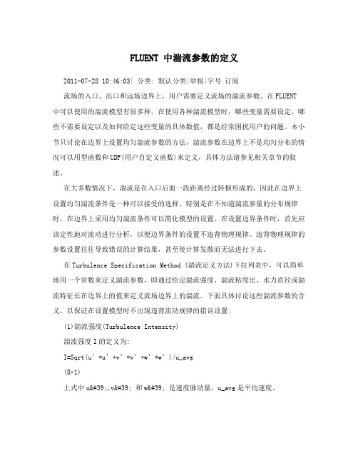
19.0 ReleaseLecture 01: Overview of EngineeringTurbulence ModelsTurbulence Modeling Using ANSYS CFDOutline•Motivation•Characteristics of Turbulent Flow−Energy Cascade−Vortex Stretching−Scales•Overview of Computational Approaches−Direct Numerical Simulation−Eddy Viscosity Models•Boussinesq Approach−Reynolds Stress Models (RSM)−Scale Resolving Simulation Models•SummaryMotivation•Turbulence is all around us−Engineering devices•Aerospace applications•Naval applications•Vehicle aerodynamics•Combustion systems−Geophysical applications•Oceanography•Meteorology and weather prediction•Environmental engineering−Biological flowsIt is critical to predict and analyze the effects of turbulence onmass, momentum and energy transportObservation by O. Reynolds –Pipe Flow with Dye Injection •Flows can be classified as either :−Laminar:•Low Reynolds number•Fluid particles path exhibit no disturbances−Transition:•Increasing Reynolds number•Orderly 2D and 3D structures appear due toflow instability−Turbulent:•Higher Reynolds number•Flow exhibits random 3D unsteady structuresCharacteristics of Turbulent Flows•Unsteady, irregular (aperiodic) motion in which transported quantities (mass, momentum, scalar species) fluctuate in time and space−The fluctuations are responsible for enhanced mixing oftransported quantities•Instantaneous fluctuations are random (unpredictable, irregular) both in space and time−Statistical averaging of fluctuations results in accountable, turbulence related transport mechanisms•Contains a wide range of eddy sizes (scales)−Typical identifiable swirling patterns−Large eddies “carry” small eddies−The behavior of large eddies is different in each flow•Sensitive to upstream history−The behavior of small eddies is more universal in natureLarge Structure Small StructuresMixing LayerLaminar SeparationTurbulent SeparationHas a patch of sand glued onto its leading surfaceBowling ball entering still water at 25ft/sTurbulence•Turbulence is important in almost all technical flows •Effects of turbulence:−Enhances mixing and entrainment −Dissipates kinetic energy into heat −Increases friction losses −Increases heat transfer−Delays flow separation under pressure gradients (see Figure)−Generates Noise −…•Cascade of Turbulence−Turbulence eddies are created at largest scales−Large eddies extract energy from mean flow −Largest eddies are of size of mixing layer thickness−Eddies get stretched and thereby reduced in size. This leads to an energy transfer to smaller and smaller eddies−Smallest eddies are then dissipated into heat by molecular viscosity−Smallest eddies are of Kolmogorov size −Wave number k is invers to eddy sizek =නκ=0∞EdκTurbulence kinetic energy is integral over wave number spectrum:Viscous DissipationLog ELog kGeneration of largest eddiesEnergy transferdk =EdκEnergy CascadeVortex Stretching•Existence of eddies implies vorticity•Vorticity is concentrated along vortex lines orbundles•Vortex lines/bundles become distorted from theinduced velocities of the larger eddies−As the end points of a vortex line randomly move apart•Vortex line increases in length but decreases in diameter•Vorticity increases because angular momentum is nearlyTurbulent Structures in free jet conserved−Most of the turbulence kinetic energy is contained withinthe largest eddies−Most of the vorticity is contained within the smallest eddies•The smallest turbulence scales dissipate turbulence kinetic energy into heat by viscosity•The two relevant quantities are therefore−The dissipation rate, e, (energy dissipated per unit time and volume)−Molecular viscosity, n•The only length-scale which can be formed from these two quantities is:η=(ν3/ε)Τ14•This scale is called Kolmogorov length scale•In technical fluids (air, water, etc.) the molecular viscosity is very low –therefore the Kolmogorov scales are very small•The largest turbulence scales are formed by turbulence production P k•All turbulence which is produced is eventually dissipated. One has therefore on average: P k≈ε•Most of the turbulence kinetic energy, k, is stored in the largest scales•The two relevant quantities for estimating the size of the large scales are therefore −The turbulence kinetic energy, k−The dissipation rate, e, (energy dissipated per unit time and volume)•The only length-scale which can be formed from these two quantities is:L t=(kΤ32/ε)•L t is often called the “Turbulence Length“ scale or the “Integral Length“ scaleResolution Challenge•Turbulence is a continumm problem and is described by the Navier Stokes equations •Resolving all scales of turbulence in a numerical simulation is called “Direct Numerical Simulation“ (DNS)•DNS is extremely expensive as the ratio of the large to the small scales as:•These scales have to be resolved in three dimensions making the space resolution ~Re t Τ94•In addition, the turbulence scales need to be resolved in time T tτ~kL t νΤ12•CPU cost therefore scales like CPU ~Re t Τ114-very expensive for high Re number flowsL t η~kL t νΤ34~Re tΤ34Example: Aircraft•Turbulence eddies determine aerodynamics ofaircraft –without turbulence, wings would stalland aircraft would crash•Dimension of aircraft ~ 100m•Dimension (thickness) of boundary layer 10mm-10cm•Dimension of smallest eddies ~10-5-10-6m!•In Direct Numerical Simulation of turbulence (DNS)all turbulence eddies would need to be resolved –Resolution problem (up to 1015-1018cells)Published in: Taraneh Sayadi; Curtis W. Hamman;Parviz Moin; Physics of Fluids2012, 24, Courtesey Center for Turbulence Research (CTR)Overview of Computational Approaches•Different approaches to simulate turbulence −DNS: direct numerical simulation•Full resolution•No modeling required→Too expensive for practical flows−LES: large eddy simulation•Large eddies directly resolved, smaller ones modeled→Less expensive than DNS, but very often still tooexpensive for practical applications−RANS: Reynolds Averaged Navier-Stokes simulation•Solution of time-averaged equations→Most widely used approach for industrial flows DNSRANSLESMixing LayerResolved vs Modeled scalesCreation of Large Scales Energy transfer –Inertial Range Dissipative Range –conversion to HeatResolvedResolvedDNSLES ModeledRANS Modeled∆DNS∆LESDirect Numerical Simulation•“DNS” is the solution of the time -dependent Navier-Stokes equations without recourse to modeling−Numerical time step size required, D t ~t•For channel example Re H = 30,800–Nuber of cells ~107–Number of time steps ~48,000–This is a very small piece of geometry and a very low Re number!−DNS is not suitable for practical industrial CFD•DNS is feasible only for simple geometries and low turbulent Reynolds numbers •DNS is a useful research toolρðU i ðt +U j ðU i ðx j =−ðp ðx i +ððx j μðU i ðx j∆t 2DCℎannel ≈0.003H Re τu τRANS Modeling•All turbulence effects are modeled −Reynolds Averaging•Transport equations for mean flow quantities are solved•All scales of turbulence are modeled•Transient solution D t is set by global unsteadiness•Introduces additional terms that must be modeled for closureConsider a point in the given flow field:u i x,t =U i x,t +u i ′x,tu'iU iu i timeuRANS Modeling -Ensemble Averaging•Ensemble (Phase ) average:•For statistically steady flows one can apply time averaging:U i Ԧx,t =Ui Ԧx,t +u′i Ԧx,twitℎU i Ԧx,t =lim N→∞1Nn=1NU inԦx,tU i Ԧx,t =U i Ԧx +u′i Ԧx,twitℎU i Ԧx =1T lim T→∞න0TU i Ԧx,t dtDeriving RANS Equations•Substitute mean and fluctuating velocities in instantaneous Navier-Stokes equations and average:•Some averaging rules:−Given •Mass-weighted (Favre) averaging used for compressible flows •For the momentum equation this means that:ρð(ሜU i +u i ′)ðt +(ሜU j +u j ′)ð(ሜU i +u i ′)ðx j =−ðp +p ′ðx i +ððx j μð(ሜU i +u i ′)ðx jΦ≡φ;φ′≡0;φψ=ΦΨ+φ′ψ′;Φψ′=0;φ′ψ′≠0,etc.−u i ′u j ′≠0φ=Φ+φ′;ψ=Ψ+ψ′RANS Equations•R eynolds A veraged N avier-S tokes equations:•New equations are identical to original except :−The transported variables,ሜU i ,r , etc., now represent the mean flow quantities −Additional terms appear:•t ij are called the Reynolds Stresses− Effectively a stress term →•t ij represent the influence of turbulence on the mean flow and are the terms to be modeled•t ij represents a symmetric tensor, so there are 6 additional unknownsρðሜU i ðt +ሜU j ðሜU i ðx j =−ðp ðx i +ððx j μðሜUi ðx j +ð−ρu i u j ðx jτij =−ρu i u j(prime notation dropped)ððx j μðሜUi ðx j−ρu i u jRANS vs LES/DNSRANS -U RANS -L RANS –T RANS –n tReal Flow with turbulent structures resolved •RANS is a verystrongsimplification•All information onturbulence is lostby averaging•Strong need formodeling•RANS modelingcan result insignfificant errorsin quantities ofinterestRANS Modeling : The Closure Problem•The components of the Reynolds-stress tensor, t ij, are unknown and have to bedetermined•The RANS models can be closed in two ways:−Eddy Viscosity Models•The components of t ij are modeled using an eddy (turbulent) viscosity µt•Reasonable approach for simple turbulent shear flows: boundary layers, round jets, mixing layers, channel flows, etc.−Reynolds-Stress Models (RSM)•The components of t ij are directly solved via transport equations•Advantageous in complex 3D flows with streamline curvature / swirl•Models are complex, computational intensive•The additional complexity does not always result in higher accuracyEddy Viscosity Models•The key concept of the Eddy Viscosity models is the Boussinesq hypothesis•This hypothesis assumes that the Reynolds Stresses can be expressed analogously to the viscous stresses, but applying a turbulent viscosity m t−Relation is drawn from analogy with molecular transport of momentum (Brownian velocities u”) velocities−m t depends on turbulence and needs to be determined from turbulence model equationsτij =−ρu i u j =2μt S ij −23μt ðU k ðx k δij −23ρkδij ;S ij =12ðU i ðx j +ðU j ðx it ij lam =−ρu i "u j "=2μS ijReynolds Stress Models (RSM)•Also known as Second Moment Closure Models (SMC)•Based on the solution of a transport equation for each of the independent Reynolds stresses t ij in combination with the e-or the w-equation•Some of these models show the proper sensitivity to swirl and system rotation,which have to be modeled explicitly in a two-equation framework•RSM models are also superior for flows in stagnation regions, where no additional modifications are required•RSM models are often much harder to handle numerically−The model can introduce a strong nonlinearity into the CFD method, leading to numericalproblems in many applicationsScale Resolving Simulation (SRS) Models •DNS –Direct Numerical Simulation−All turbulence scales are resolved in time and space−Extremely expensive as Reynolds number increases•LES –Large Eddy Simulation−Resolves larger eddies; models smaller ones−Inherently unsteady, D t dictated by smallest resolved eddies•Hybrid SRS Models−Combine features of classical RANS formulation with elements of LES method −SBES•Physically based on blend of the RANS and LES models−WMLES−ZonalSRS refers to methods, which resolved at least aportion of theturbulence spectrum in at least a part of the flowdomainImpact of Turbulence Models•The usage of RANS models in CFD reduces the required computing power by many orders of magnitude relative to DNS−E.g. For external airplane simulation the reduction is of order ~1010or larger!•It is not realistic to expect that such a strong simplification will always result in small errors in the solution•Depending on the application, RANS models can introduce substantial errors into the simulation•Errors can be reduced by:−Optimal selection of turbulence model and sub-models−High quality grids and optimal numerical settings−Investment of more computing power by using Scale-Resolving Simulations (SRS)Turbulence Models in Fluent & CFX•A large number of turbulence models is available, some for very specificapplications, others can be applied to a wider class of flows with a reasonable degree of confidence•Many of the models available are there for historical reasons•The large number of turbulence models is often confusing to the user and a optimal selection is difficult•In addition, there are many sub-options which can/should be activated by the user in certain scenarios•ANSYS tries to consolidate the model offering as much as possible and setstrong defaults•The user community needs to move along and eventually abandon legacymodelsSummary•Turbulent flows are inherently unsteady, three-dimensional and irregular•A broad range of time and length scales exist in turbulent flows•Turbulent flows are governed by the Navier-Stokes equations, but the need to resolve all scales from the dissipative (Kolmogorov) scales to the mean flow scales makesdirect simulation too expensive to be feasible for industrial applications•Reynolds averaging is one of the approaches used to eliminate the turbulence scales.The application of this approach leads to the Reynolds Averaged Navier-Stokes (RANS) equations•The Reynolds stress terms in the RANS equation require modelling in order to obtain a closed system of equations•Scale resolving simulation opens a path to include at least some resolved scales into the simulationAPPENDIXNon Dimensional Numbers in Turbulent flows。
fluent中多孔介质设置问题和算例

经过痛苦的一段经历,终于将局部问题真相大白,为了使保位某某不再经过我之痛苦,现在将本人多孔介质经验公布如下,希望各位能加精:1。
Gambit中划分网格之后,定义需要做为多孔介质的区域为fluid,与缺省的fluid分别开来,再定义其名称,我习惯将名称定义为porous;2。
在fluent中定义边界条件define-boundary condition-porous(刚定义的名称),将其设置边界条件为fluid,点击set按钮即弹出与fluid边界条件一样的对话框,选中porous zone与laminar复选框,再点击porous zone标签即出现一个带有滚动条的界面;3。
porous zone设置方法:1〕定义矢量:二维定义一个矢量,第二个矢量方向不用定义,是与第一个矢量方向正交的;三维定义二个矢量,第三个矢量方向不用定义,是与第一、二个矢量方向正交的;〔如何知道矢量的方向:打开grid图,看看X,Y,Z的方向,如果是X向,矢量为1,0,0,同理Y向为0,1,0,Z向为0,0,1,如果所需要的方向与坐标轴正向相反,如此定义矢量为负〕圆锥坐标与球坐标请参考fluent帮助。
2〕定义粘性阻力1/a与内部阻力C2:请参看本人上一篇博文“终于搞清fluent中多孔粘性阻力与内部阻力的计算方法〞,此处不赘述;3〕如果了定义粘性阻力1/a与内部阻力C2,就不用定义C1与C0,因为这是两种不同的定义方法,C1与C0只在幂率模型中出现,该处保持默认就行了;4〕定义孔隙率porousity,默认值1表示全开放,此值按实验测值填写即可。
完了,其他设置与普通k-e或RSM一样。
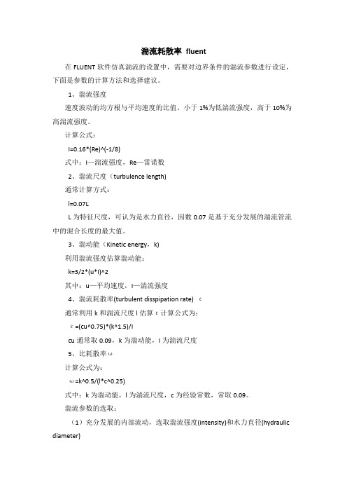
总结一下,与君共享!Tutorial 7. Modeling Flow Through Porous MediaIntroductionMany industrial applications involve the modeling of flow through porous media, such as filters, catalyst beds, and packing. This tutorial illustrates how to set up and solve a problem involving gas flow through porous media.The industrial problem solved here involves gas flow through a catalytic converter. Catalytic converters are monly used to purify emissions from gasoline and diesel engines by converting environmentally hazardous exhaust emissions to acceptable substances.Examples of such emissions include carbon monoxide (CO), nitrogen oxides (NOx), and unburned hydrocarbon fuels. These exhaust gas emissions are forced through a substrate, which is a ceramic structure coated with a metal catalyst such as platinum or palladium.The nature of the exhaust gas flow is a very important factor in determining the performance of the catalytic converter. Of particular importance is the pressure gradient and velocity distribution through the substrate. Hence CFD analysis is used to design efficient catalytic converters: by modeling the exhaust gas flow, the pressure drop and the uniformity of flow through the substrate can be determined. In this tutorial, FLUENT is used to model the flow of nitrogen gas through a catalytic converter geometry, so that the flow field structure may be analyzed.This tutorial demonstrates how to do the following:_ Set up a porous zone for the substrate with appropriate resistances._ Calculate a solution for gas flow through the catalytic converter using the pressure based solver. _ Plot pressure and velocity distribution on specified planes of the geometry._ Determine the pressure drop through the substrate and the degree of non-uniformity of flow through cross sections of the geometry using X-Y plots and numerical reports.Problem DescriptionThe catalytic converter modeled here is shown in Figure 7.1. The nitrogen flows in through the inlet with a uniform velocity of 22.6 m/s, passes through a ceramic monolith substrate with square shaped channels, and then exits through the outlet.While the flow in the inlet and outlet sections is turbulent, the flow through the substrate is laminar and is characterized by inertial and viscous loss coefficients in the flow (X) direction. The substrate is impermeable in other directions, which is modeled using loss coefficients whose values are three orders of magnitude higher than in the X direction.Setup and SolutionStep 1: Grid1. Read the mesh file (catalytic converter.msh).File /Read /Case...2. Check the grid. Grid /CheckFLUENT will perform various checks on the mesh and report the progress in the console. Make sure that the minimum volume reported is a positive number.3. Scale the grid.Grid! Scale...(a) Select mm from the Grid Was Created In drop-down list.(b) Click the Change Length Units button. All dimensions will now be shown in millimeters.(c) Click Scale and close the Scale Grid panel.4. Display the mesh. Display /Grid...(a) Make sure that inlet, outlet, substrate-wall, and wall are selected in the Surfaces selection list.(b) Click Display.(c) Rotate the view and zoom in to get the display shown in Figure 7.2.(d) Close the Grid Display panel.The hex mesh on the geometry contains a total of 34,580 cells.Step 2: Models1. Retain the default solver settings. Define /Models /Solver...2. Select the standard k-ε turbulence model. Define/ Models /Viscous...Step 3: Materials1. Add nitrogen to the list of fluid materials by copying it from the Fluent Database for materials.Define /Materials...(a) Click the Fluent Database... button to open the Fluent Database Materials panel.i. Select nitrogen (n2) from the list of Fluent Fluid Materials.ii. Click Copy to copy the information for nitrogen to your list of fluid materials. iii. Close the Fluent Database Materials panel.(b) Close the Materials panel.Step 4: Boundary Conditions. Define /Boundary Conditions...1. Set the boundary conditions for the fluid (fluid).(a) Select nitrogen from the Material Name drop-down list.(b) Click OK to close the Fluid panel.2. Set the boundary conditions for the substrate (substrate).(a) Select nitrogen from the Material Name drop-down list.(b) Enable the Porous Zone option to activate the porous zone model.(c) Enable the Laminar Zone option to solve the flow in the porous zone without turbulence.(d) Click the Porous Zone tab.i. Make sure that the principal direction vectors are set as shown in Table7.1. Use the scroll bar to access the fields that are not initially visible in the panel.ii. Enter the values in Table 7.2 for the Viscous Resistance and Inertial Resistance. Scroll down to access the fields that are not initially visible in the panel.(e) Click OK to close the Fluid panel.3. Set the velocity and turbulence boundary conditions at the inlet (inlet).(a) Enter 22.6 m/s for the Velocity Magnitude.(b) Select Intensity and Hydraulic Diameter from the Specification Method dropdown list in the Turbulence group box.(c) Retain the default value of 10% for the Turbulent Intensity.(d) Enter 42 mm for the Hydraulic Diameter.(e) Click OK to close the Velocity Inlet panel.4. Set the boundary conditions at the outlet (outlet).(a) Retain the default setting of 0 for Gauge Pressure.(b) Select Intensity and Hydraulic Diameter from the Specification Method dropdown list in the Turbulence group box.(c) Enter 5% for the Backflow Turbulent Intensity.(d) Enter 42 mm for the Backflow Hydraulic Diameter.(e) Click OK to close the Pressure Outlet panel.5. Retain the default boundary conditions for the walls (substrate-wall and wall) and close the Boundary Conditions panel.Step 5: Solution1. Set the solution parameters. Solve /Controls /Solution...(a) Retain the default settings for Under-Relaxation Factors.(b) Select Second Order Upwind from the Momentum drop-down list in the Discretization group box.(c) Click OK to close the Solution Controls panel.2. Enable the plotting of residuals during the calculation. Solve/Monitors /Residual...(a) Enable Plot in the Options group box.(b) Click OK to close the Residual Monitors panel.3. Enable the plotting of the mass flow rate at the outlet.Solve / Monitors /Surface...(a) Set the Surface Monitors to 1.(b) Enable the Plot and Write options for monitor-1, and click the Define... button to open the Define Surface Monitor panel.i. Select Mass Flow Rate from the Report Type drop-down list.ii. Select outlet from the Surfaces selection list.iii. Click OK to close the Define Surface Monitors panel.(c) Click OK to close the Surface Monitors panel.4. Initialize the solution from the inlet. Solve /Initialize /Initialize...(a) Select inlet from the pute From drop-down list.(b) Click Init and close the Solution Initialization panel.5. Save the case file (catalytic converter.cas). File /Write /Case...6. Run the calculation by requesting 100 iterations. Solve /Iterate...(a) Enter 100 for the Number of Iterations.(b) Click Iterate.The FLUENT calculation will converge in approximately 70 iterations. By this point the mass flow rate monitor has attended out, as seen in Figure 7.3.(c) Close the Iterate panel.7. Save the case and data files (catalytic converter.cas and catalytic converter.dat).File /Write /Case & Data...Note: If you choose a file name that already exists in the current folder, FLUENTwill prompt you for confirmation to overwrite the file.Step 6: Post-processing1. Create a surface passing through the centerline for post-processing purposes.Surface/Iso-Surface...(a) Select Grid... and Y-Coordinate from the Surface of Constant drop-down lists.(b) Click pute to calculate the Min and Max values.(c) Retain the default value of 0 for the Iso-Values.(d) Enter y=0 for the New Surface Name.(e) Click Create.2. Create cross-sectional surfaces at locations on either side of the substrate, as well as at its center.Surface /Iso-Surface...(a) Select Grid... and X-Coordinate from the Surface of Constant drop-down lists.(b) Click pute to calculate the Min and Max values.(c) Enter 95 for Iso-Values.(d) Enter x=95 for the New Surface Name.(e) Click Create.(f) In a similar manner, create surfaces named x=130 and x=165 with Iso-Values of 130 and 165, respectively. Close the Iso-Surface panel after all the surfaces have been created.3. Create a line surface for the centerline of the porous media.Surface /Line/Rake...(a) Enter the coordinates of the line under End Points, using the starting coordinate of (95, 0, 0) and an ending coordinate of (165, 0, 0), as shown.(b) Enter porous-cl for the New Surface Name.(c) Click Create to create the surface.(d) Close the Line/Rake Surface panel.4. Display the two wall zones (substrate-wall and wall). Display /Grid...(a) Disable the Edges option.(b) Enable the Faces option.(c) Deselect inlet and outlet in the list under Surfaces, and make sure that only substrate-wall and wall are selected.(d) Click Display and close the Grid Display panel.(e) Rotate the view and zoom so that the display is similar to Figure 7.2.5. Set the lighting for the display. Display /Options...(a) Enable the Lights On option in the Lighting Attributes group box.(b) Retain the default selection of Gourand in the Lighting drop-down list.(c) Click Apply and close the Display Options panel.6. Set the transparency parameter for the wall zones (substrate-wall and wall).Display/Scene...(a) Select substrate-wall and wall in the Names selection list.(b) Click the Display... button under Geometry Attributes to open the Display Properties panel.i. Set the Transparency slider to 70.ii. Click Apply and close the Display Properties panel.(c) Click Apply and then close the Scene Description panel.7. Display velocity vectors on the y=0 surface.Display /Vectors...(a) Enable the Draw Grid option. The Grid Display panel will open.i. Make sure that substrate-wall and wall are selected in the list under Surfaces.ii. Click Display and close the Display Grid panel.(b) Enter 5 for the Scale.(c) Set Skip to 1.(d) Select y=0 from the Surfaces selection list.(e) Click Display and close the Vectors panel.The flow pattern shows that the flow enters the catalytic converter as a jet, with recirculation on either side of the jet. As it passes through the porous substrate, it decelerates and straightens out, and exhibits a more uniform velocity distribution.This allows the metal catalyst present in the substrate to be more effective.Figure 7.4: Velocity Vectors on the y=0 Plane8. Display filled contours of static pressure on the y=0 plane.Display /Contours...(a) Enable the Filled option.(b) Enable the Draw Grid option to open the Display Grid panel.i. Make sure that substrate-wall and wall are selected in the list under Surfaces.ii. Click Display and close the Display Grid panel.(c) Make sure that Pressure... and Static Pressure are selected from the Contours of drop-down lists.(d) Select y=0 from the Surfaces selection list.(e) Click Display and close the Contours panel.Figure 7.5: Contours of the Static Pressure on the y=0 planeThe pressure changes rapidly in the middle section, where the fluid velocity changes as it passes through the porous substrate. The pressure drop can be high, due to the inertial and viscous resistance of the porous media. Determining this pressure drop is a goal of CFD analysis. In the next step, you will learn how to plot the pressure drop along the centerline of the substrate.9. Plot the static pressure across the line surface porous-cl.Plot /XY Plot...(a) Make sure that the Pressure... and Static Pressure are selected from the Y Axis Function drop-down lists.(b) Select porous-cl from the Surfaces selection list.(c) Click Plot and close the Solution XY Plot panel.Figure 7.6: Plot of the Static Pressure on the porous-cl Line SurfaceIn Figure 7.6, the pressure drop across the porous substrate can be seen to be roughly 300 Pa.10. Display filled contours of the velocity in the X direction on the x=95, x=130 and x=165 surfaces.Display /Contours...(a) Disable the Global Range option.(b) Select Velocity... and X Velocity from the Contours of drop-down lists.(c) Select x=130, x=165, and x=95 from the Surfaces selection list, and deselect y=0.(d) Click Display and close the Contours panel.The velocity profile bees more uniform as the fluid passes through the porous media. The velocity is very high at the center (the area in red) just before the nitrogen enters the substrate and then decreases as it passes through and exits the substrate. The area in green, which corresponds to a moderate velocity, increases in extent.Figure 7.7: Contours of the X Velocity on the x=95, x=130, and x=165 Surfaces11. Use numerical reports to determine the average, minimum, and maximum of the velocity distribution before and after the porous substrate.Report /Surface Integrals...(a) Select Mass-Weighted Average from the Report Type drop-down list.(b) Select Velocity and X Velocity from the Field Variable drop-down lists.(c) Select x=165 and x=95 from the Surfaces selection list.(d) Click pute.(e) Select Facet Minimum from the Report Type drop-down list and click pute again.(f) Select Facet Maximum from the Report Type drop-down list and click pute again.(g) Close the Surface Integrals panel.The numerical report of average, maximum and minimum velocity can be seen in the main FLUENT console, as shown in the following example:word21 /21The spread between the average, maximum, and minimum values for X velocity gives the degree to which the velocity distribution is non-uniform. You can also use these numbers to calculate the velocity ratio (i.e., the maximum velocity divided by the mean velocity) and the space velocity (i.e., the product of the mean velocity and the substrate length).Custom field functions and UDFs can be also used to calculate more plex measures of non-uniformity, such as the standard deviation and the gamma uniformity index.SummaryIn this tutorial, you learned how to set up and solve a problem involving gas flow through porous media in FLUENT. You also learned how to perform appropriate post-processing to investigate the flow field, determine the pressure drop across the porous media and non-uniformity of the velocity distribution as the fluid goes through the porous media.Further ImprovementsThis tutorial guides you through the steps to reach an initial solution. You may be able to obtain a more accurate solution by using an appropriate higher-order discretization scheme and by adapting the grid. Grid adaption can also ensure that the solution is independent of the grid. These steps are demonstrated in Tutorial 1.。
fluent相关问题汇总

1、实体、实面与虚体、虚面的区别在建模中,经常会遇到实...与虚...,而且虚体的计算域好像也可以进行计算并得到所需的结果,对二者的根本区别及在功能上的不同对于求解是没有任何区别的,只要你能在虚体或者实体上划分你需要的网格Gambit的实体和虚体在生成网格和计算的时候对于结果没有任何影响,实体和虚体的主要区别有以下几点:1.实体可以进行布尔运算但是虚体不能,虽然不能进行布尔运算,但是虚体存在merge,split等功能;2.实体运算在很多cad软件里面都有,但是虚体是gambit的一大特色,有了虚体以后,Gambit的建模和网格生成的灵活性增加了很多。
3.在网格生成的过程中,如果有几个相对比较平坦的面,你可以把它们通过merge合成一个,这样,作网格的时候,可以节省步骤,对于曲率比较大的面,可能生成的网格质量不好,这时候,你可以采取用split的方式把它划分成几个小面以提高网格质量。
对于虚体生成的计算网格,和实体生成的计算网格,在计算的时候没有区别,关键是看网格生成的质量如何,与实体虚体无关。
经常在作复杂模型计算的时候,大部分都是用的虚体,特别是从其他的建模软件里面导进来的复杂模型,基本上不能够生成实体。
至于计算的效果如何,与Fluent的设置和网格的质量有关,与模型无关。
2、什么叫问题的初始化?在FLUENT中初始化的方法对计算结果有什么样的影响?初始化中的“patch”怎么理解?问题的初始化就是在做计算时,给流场一个初始值,包括压力、速度、温度和湍流系数等。
理论上,给的初始场对最终结果不会产生影响,因为随着跌倒步数的增加,计算得到的流场会向真实的流场无限逼近,但是,由于Fluent等计算软件存在像离散格式精度(会产生离散误差)和截断误差等问题的限制,如果初始场给的过于偏离实际物理场,就会出现计算很难收敛,甚至是刚开始计算就发散的问题。
因此,在初始化时,初值还是应该给的尽量符合实际物理现象。
这就要求我们对要计算的物理场,有一个比较清楚的理解。
fluent算例模拟燃烧
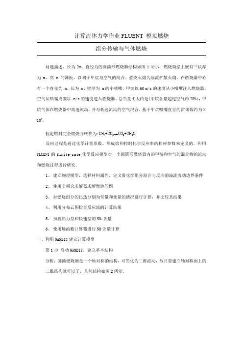
计算流体力学作业FLUENT 模拟燃烧问题描述:长为2m、直径为的圆筒形燃烧器结构如图1所示,燃烧筒壁上嵌有三块厚为 m,高 m的薄板,以利于甲烷与空气的混合。
燃烧火焰为湍流扩散火焰。
在燃烧器中心有一个直径为 m、长为 m、壁厚为 m的小喷嘴,甲烷以60 m/s的速度从小喷嘴注入燃烧器。
空气从喷嘴周围以 m/s的速度进入燃烧器。
总当量比大约是(甲烷含量超过空气约28%),甲烷气体在燃烧器中高速流动,并与低速流动的空气混合,基于甲烷喷嘴直径的雷诺数约为×103。
假定燃料完全燃烧并转换为:CH4+2O2→CO2+2H2O反应过程是通过化学计量系数、形成焓和控制化学反应率的相应参数来定义的。
利用FLUENT的finite-rate化学反应模型对一个圆筒形燃烧器内的甲烷和空气的混合物的流动和燃烧过程进行研究。
1、建立物理模型,选择材料属性,定义带化学组分混合与反应的湍流流动边界条件2、使用非耦合求解器求解燃烧问题3、对燃烧组分的比热分别为常量和变量的情况进行计算,并比较其结果4、利用分布云图检查反应流的计算结果5、预测热力型和快速型的NO X含量6、使用场函数计算器进行NO含量计算一、利用GAMBIT建立计算模型第1步启动GAMBIT,建立基本结构分析:圆筒燃烧器是一个轴对称的结构,可简化为二维流动,故只要建立轴对称面上的二维结构就可以了,几何结构如图2所示。
(1)建立新文件夹在F盘根目录下建立一个名为combustion的文件夹。
(2)启动GAMBIT(3)创建对称轴①创建两端点。
A(0,0,0),B(2,0,0)②将两端点连成线(4)创建小喷嘴及空气进口边界①创建C、D、E、F、G点②连接AC、CD、DE、DF、FG。
(5)创建燃烧筒壁面、隔板和出口①创建H、I、J、K、L、M、N点(y轴为,z轴为0)。
②将H、I、J、K、L、M、N向Y轴负方向复制,距离为板高度。
③连接GH、HO、OP、PI、IJ、JQ、QR、RK、KL、LS、ST、TM、MN、NB。
FLUENT软件操作界面中英文对照

FLUENT软件操作界面中英文对照编辑整理:尊敬的读者朋友们:这里是精品文档编辑中心,本文档内容是由我和我的同事精心编辑整理后发布的,发布之前我们对文中内容进行仔细校对,但是难免会有疏漏的地方,但是任然希望(FLUENT软件操作界面中英文对照)的内容能够给您的工作和学习带来便利。
同时也真诚的希望收到您的建议和反馈,这将是我们进步的源泉,前进的动力。
本文可编辑可修改,如果觉得对您有帮助请收藏以便随时查阅,最后祝您生活愉快业绩进步,以下为FLUENT软件操作界面中英文对照的全部内容。
FLUENT 软件操作界面中英文对照File 文件Grid 网格Models 模型 : solver 解算器Read 读取文件:scheme 方案 journal 日志profile 外形Write 保存文件Import:进入另一个运算程序Interpolate :窜改,插入Hardcopy : 复制,Batch options 一组选项Save layout 保存设计Pressure based 基于压力Density based 基于密度implicit 隐式, explicit 显示Space 空间:2D,axisymmetric(转动轴),axisymmetric swirl (漩涡转动轴);Time时间:steady 定常,unsteady 非定常Velocity formulation 制定速度:absolute绝对的; relative 相对的Gradient option 梯度选择:以单元作基础;以节点作基础;以单元作梯度的最小正方形。
Porous formulation 多孔的制定:superticial velocity 表面速度;physical velocity 物理速度;solver求解器Multiphase 多相 energy 能量方程Visous 湍流层流,流态选择Radiation 辐射Species 种类,形式(燃烧和化学反应)Discrete phase 离散局面Solidification & melting (凝固/熔化)Acoustics 声音学:broadband noise sources多频率噪音源models模型Materials 定义物质性质Phase 阶段,相Operating conditions 操作压力条件Boundary conditions 边界条件Periodic conditions 周期性条件Grid interfaces 两题边界的表面网格Dynamic mesh 动力学的网孔Mixing planes 混合飞机?混合翼面?Turbo topology 涡轮拓扑Injections 注射DTRM rays DTRM射线Custom field functions 常用函数Profiles 外观,Units 单位User-defined 用户自定义materials 材料Name 定义物质的名称 chemical formula 化学反应式 material type 物质类型(液体,固体)Fluent fluid materials 流动的物质 mixture 混合物order materials by 根据什么物质(名称/化学反应式)Fluent database 流体数据库 user-defined database 用户自定义数据库Propertles 物质性质从上往下分别是密度比热容导热系数粘滞系数Operating conditions操作条件操作压力设置:operating pressure操作压力reference pressure location 参考压力位置gravity 重力,地心引力gravitational Acceleration 重力加速度operating temperature 操作温度variable—density parameters 可变密度的参数specified operating density 确切的操作密度Boundary conditions边界条件设置Fluid定义流体Zone name区域名 material name 物质名 edit 编辑Porous zone 多空区域 laminar zone 薄层或者层状区域 source terms (源项?)Fixed values 固定值motion 运动rotation—axis origin旋转轴原点Rotation—axis direction 旋转轴方向Motion type 运动类型: stationary静止的; moving reference frame 移动参考框架; Moving mesh 移动网格Porous zone 多孔区Reaction 反应Source terms (源项)Fixed values 固定值velocity—inlet速度入口Momentum 动量 thermal 温度 radiation 辐射 species 种类DPM DPM模型(可用于模拟颗粒轨迹) multipahse 多项流UDS(User define scalar 是使用fluent求解额外变量的方法)Velocity specification method 速度规范方法: magnitude,normal to boundary 速度大小,速度垂直于边界;magnitude and direction 大小和方向;components 速度组成?Reference frame 参考系:absolute绝对的;Relative to adjacent cell zone 相对于邻近的单元区Velocity magnitude 速度的大小Turbulence 湍流Specification method 规范方法k and epsilon K—E方程:1 Turbulent kinetic energy湍流动能;2 turbulent dissipation rate 湍流耗散率Intensity and length scale 强度和尺寸: 1湍流强度 2 湍流尺度=0.07L(L为水力半径)intensity and viscosity rate强度和粘度率:1湍流强度2湍流年度率intensity and hydraulic diameter强度与水力直径:1湍流强度;2水力直径pressure-inlet压力入口Gauge total pressure 总压supersonic/initial gauge pressure 超音速/初始表压constant常数direction specification method 方向规范方法:1direction vector方向矢量;2 normal to boundary 垂直于边界mass—flow—inlet质量入口Mass flow specification method 质量流量规范方法:1 mass flow rate 质量流量;2 massFlux 质量通量 3mass flux with average mass flux 质量通量的平均通量supersonic/initial gauge pressure 超音速/初始表压direction specification method 方向规范方法:1direction vector方向矢量;2 normal to boundary 垂直于边界Reference frame 参考系:absolute绝对的;Relative to adjacent cell zone 相对于邻近的单元区pressure-outlet压力出口Gauge pressure表压backflow direction specification method 回流方向规范方法:1direction vector方向矢量;2 normal to boundary 垂直于边界;3 from neighboring cell 邻近单元Radial equilibrium pressure distribution 径向平衡压力分布Target mass flow rate 质量流量指向pressure-far—field压力远程Mach number 马赫数 x-component of flow direction X分量的流动方向outlet自由出流Flow rate weighting 流量比重inlet vent进口通风Loss coeffcient 损耗系数 1 constant 常数;2 piecewise—linear分段线性;3piecewise-polynomial 分段多项式;4 polynomial 多项式EditPolynomial Profile高次多项式型线Define 定义 in terms of 在一下方面 normal-velocity 正常速度 coefficients系数intake Fan进口风扇Pressure jump 压力跃 1 constant 常数;2 piecewise—linear分段线性;3piecewise—polynomial 分段多项式;4 polynomial 多项式exhaust fan排气扇对称边界(symmetry)周期性边界(periodic)Wall固壁边界adjicent cell zone相邻的单元区Wall motion 室壁运动:stationary wall 固定墙Shear condition 剪切条件: no slip 无滑;specified shear 指定的剪切;specularity coefficients 镜面放射系数 marangoni stress 马兰格尼压力?Wall roughness 壁面粗糙度:roughness height 粗糙高度 roughness constant粗糙常数Moving wall移动墙壁Translational 平移rotational 转动components 组成Solve/controls/solution 解决/控制/解决方案Equations 方程 under—relaxation factors 松弛因子: body forces 体积力Momentum动量 turbulent kinetic energy 湍流动能turbulent dissipation rate湍流耗散率Turbulent viscosity 湍流粘度 energy 能量Pressure-velocity coupling 压力速度耦合: simple ,simplec,plot和coupled是4种不同的算法。
(整理)FLUENT边界条件(2)—湍流设置.

FLUENT边界条件(2)—湍流设置(fluent教材—fluent入门与进阶教程于勇第九章)Fluent:湍流指定方法(Turbulence Specification Method)2009-09-16 20:50使用Fluent时,对于velocity inlet边界,涉及到湍流指定方法(Turbulence Specification Method),其中一项是Intensity and Hydraulic Diameter (强度和水利直径),本文对其进行论述。
其下参数共两项,(1)是Turbulence Intensity,确定方法如下:I=0.16/Re_DH^0.125 (1)其中Re_DH是Hydraulic Diameter(水力直径)的意思,即式(1)中的雷诺数是以水力直径为特征长度求出的。
雷诺数Re_DH=u×DH/υ(2)u为流速,DH为水利直径,υ为运动粘度。
水利直径见(2)。
(2)水利直径水力直径是水力半径的二倍,水力半径是总流过流断面面积与湿周之比。
水力半径R=A/X (3)其中,A为截面积(管子的截面积)=流量/流速X为湿周(字面理解水流过各种形状管子外圈湿一周的周长)例如:方形管的水利半径R=ab/2(a+b)水利直径DH=2×R (4)举例如下:如果水流速度u=10m/s,圆形管路直径2cm,水的运动粘度为1×10-6 m2/s。
则DH=2×3.14*r^2/(2*3.14*r)=2*3.14*0.01^2/(3.14*0.02)=0.01 r为圆管半径Re_DH=u×DH/υ=10*0.02/10e-6=20000I=0.16/Re_DH^0.125=0.16/20000^0.125=0.0463971424017634≈5%水力半径:润湿周长横截面积=h r , 水力直径:h h r 4D =对圆管而言,管道直径和水力直径是一回事。
fluent边界条件的含义
Fluent教程—流动入口、出口边界条件(一)时刻:2021-03-15 17:19:51 来源:查看:2254 评论:0FLUENT提供了10种类型的流动进、出口条件,它们别离是:★一样形式:★可紧缩流动:压力入口质量入口压力出口压力远场★不可紧缩流动:★特殊进出口条件:速度入口入口通分,出口通风自由流出吸气风扇,排气风扇1,速度入口(velocity-inlet):给出入口速度及需要计算的所有标量值。
该边界条件适用于不可紧缩流动问题,对可紧缩问题不适用,不然该入口边界条件会使入口处的总温或总压有必然的波动。
2,压力入口(pressure-inlet):给出入口的总压和其它需要计算的标量入口值。
对计算可压不可压问题都适用。
3,质量流入口(mass-flow-inlet):要紧用于可紧缩流动,给出入口的质量流量。
关于不可紧缩流动,没有必要给出该边界条件,因为密度是常数,咱们能够用速度入口条件。
4,压力出口(pressure-outlet):给定流动出口的静压。
关于有回流的出口,该边界条件比outflow 边界条件更易收敛。
该边界条件只能用于模拟亚音速流动。
5,压力远场(pressure-far-field):该边界条件只对可紧缩流动适合。
6,自由出流(outflow):该边界条件用以模拟在求解问题之前,无法明白出口速度或压力;出口流动符合完全进展条件,出口处,除压力之外,其它参量梯度为零。
但并非是所有问题都适合,有三种情形不能用自由出流边界条件:包括压力入口条件;可紧缩流动问题;有密度转变的非稳固流动(即便是不可紧缩流动)。
7,入口通风(inlet vent):入口风扇条件需要给定一个损失系数,流动方向和环境总压和总温。
8,入口风扇(intake fan):入口风扇条件需要给定压降,流动方向和环境总压和总温。
9,出口通风(out let vent):排出风扇给定损失系数和环境静压和静温。
10, 排气扇(exhaust fan):排除风扇给定压降,环境静压。
FLUENT中组分输运及化学反应燃烧模拟

混合分数定义
混合分数, f, 写成元素的质量分数形式:
f Zk Zk,O Zk,F Zk,O
其处中的,值。Zk 是元素k的质量分数 ;下标 F 和O 表示燃料和氧化剂进口流
对于简单的 fuel/oxidizer系统, 混合物分数代表计算控制体里的燃料 质量分数.
平衡化学的 PDF模型 层流火焰面模型
进展变量模型
Zimont 模型
有限速率模型
用总包机理反应描述化学反应过程. 求解化学组分输运方程.
求解当地时间平均的各个组分的质量分数, mj.
组分 j的源项 (产生或消耗)是机理中所有k个反应的净反应速率 :
Rj Rjk k
R、jk混(第合k或个涡化旋学破反碎应(生E成BU或)消速耗率的的j 组小分值)。是.根据 Arrhenius速率公式
p(f) can be used to compute time-averaged values of variables that
depend on the mixture fraction, f:
i
1 0
p
(
f
)
i( f )d f
Species mole fractions
Temperature, density
的燃烧过程。.
计算连续相流动场 计算颗粒轨道
更新连续相源项
颗粒弥散: 随机轨道模型
Monte-Carlo方法模拟湍流颗粒弥散 (discrete random walks)
颗粒运动计算中考虑气体的平均速度及随机湍流脉 动速度的影响。
每个轨道包含了一群具有相同特性的颗粒,如相同 的初始直径,密度等.
Fluent经典教材.5.turbulence
ρU i
Convection
Generation
Diffusion
Dissipation Rate
ε2 ε ε ε U j U i U j ρU i + + = C1ε t C 2ε ρ ( t σ ε ) k x x xi x j i xi xi k i
D5
Fluent Inc. 6/18/2010
Fluent Software Training TRN-98-006
Choices to be Made
Flow Physics Computational Resources
Turbulence Model & Near-Wall Treatment
D9 Fluent Inc. 6/18/2010
Fluent Software Training TRN-98-006
One-Equation Model: Spalart-Allmaras
Designed specifically for aerospace applications involving wallbounded flows.
One Equation Model: Spalart-Allmaras
Turbulent viscosity is determined from:
~ (ν /ν )3 ~ t = ρν ~ 3 (ν /ν ) + cν 13
~ ν is determined from the modified viscosity transport equation:
Fluent Turbulence Notes
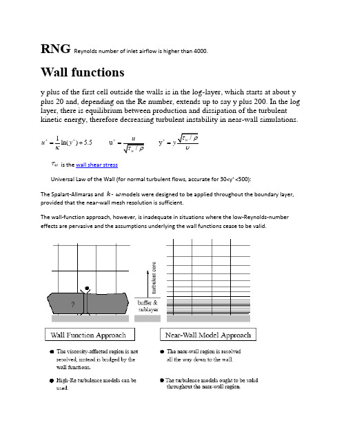
RNG Reynolds number of inlet airflow is higher than 4000.Wall functionsy plus of the first cell outside the walls is in the log-layer, which starts at about y plus 20 and, depending on the Re number, extends up to say y plus 200. In the log layer, there is equilibrium between production and dissipation of the turbulentkinetic energy, therefore decreasing turbulent instability in near-wall simulations.1ln() 5.5 uu yκ++++=+==is the wall shear stressUniversal Law of the Wall (for normal turbulent flows, accurate for 30<y+ <500):The Spalart-Allmaras and - models were designed to be applied throughout the boundary layer, provided that the near-wall mesh resolution is sufficient.The wall-function approach, however, is inadequate in situations where the low-Reynolds-number effects are pervasive and the assumptions underlying the wall functions cease to be valid.•Do not need as many elements near the wall•For the Universal Law of the Wall:•Closest element - not too near the wall: standard use: y+>11.225 (and y+<200)•y = distance from wall to node closest to wall•u = velocity at node closest to the wall•Non-equilibrium wall functions (two layer model)•larger pressure gradients•more turbulence production near the walls•separation, reattachment, impingement•first element in turbulent boundary layer• 30<y+<200Limitations of wall functions which do not model:•important low Re effects - small gaps or highly viscous flows•transpiration (blowing or sucking)•strong separation•strong natural convection effects (buoyancy effects are included but there is still some uncertainty)•strongly 3D flow near the wall•Enhanced wall treatment – 2 layer model•Additional models for detailed resolution of the laminar sub-layer•Can be used with fine meshes y+~1 and near wall meshes y+>11.225•Only with smooth walls• -specific dissipation, describes scale of the turbulence•Low Reynolds number model•Can be used for both high and low Re•Does not use wall functions•Requires much finer grid•Wall element should have–y+<5–y+~1 is best–Need more elements near the wall(default=0.5 is value for uniform sand grains) •k- models–Standard wall functions•30<y+<200–Non-Equilibrium Wall Functions•30< y+<200–Enhanced wall functions•y+<1 or y+>20•Seems to work for all values•does not have a wall roughness option•k- models•y+<5 (<1 better)Because of the capability to partly account for the effects of pressure gradients and departure from equilibrium, the non-equilibrium wall functions are recommended for use in complex flows involving separation, reattachment, and impingement where the mean flow and turbulence are subjected to severe pressure gradients and change rapidly. In such flows, improvements can be obtained, particularly in the prediction of wall shear (skin-friction coefficient) and heat transfer (Nusselt or Stanton number).。
fluent下使用非牛顿流体

fluent下使用非牛顿流体2009-11-24 10:471、非牛顿流体:剪应力与剪切应变率之间满足线性关系的流体称为牛顿流体,而把不满足线性关系的流体称为非牛顿流体。
2、fluent中使用非牛顿流体a、层流状态:直接在材料物性下设置材料的粘度,设置其为非牛顿流体。
b、湍流状态fluent在设置湍流模型后,会自动将材料的非牛顿流体性质直接改成了牛顿流体,因此需要做一些修改。
最基本的方式有两种:1、打开隐藏的湍流模型下非牛顿流体功能;2,直接利用UDF宏DEFINE_PROPERTY定义3、打开隐藏的湍流模型下非牛顿流体功能方法为:(1)在湍流模型中选择标准的k-e模型;(2)在Fluent窗口输入命令:define/models/viscous/turbulence-expert/turb-non-newtonian 然后回车。
(3)输入:y 然后回车。
4、利用DEFINE_PROPERTY宏A:这是一个自定义材料的粘度程序如下,也许对你有帮助。
在记事本中编辑的,另存为“visosity1.c"#include "udf.h"DEFINE_PROPERTY(cell_viscosity, cell, thread){real mu_lam;real trial;rate=CELL_STRAIN_RATE_MAG(cell, thread);real temp=C_T(cell, thread);mu_lam=1.e12;{if(rate>1.0e-4 && rate<1.e5)trial=12830000./rate*log(pow((rate*exp(17440.46/temp)/1.53514 6e8),0.2817)+pow((1.+pow((rate*exp(17440.46/temp)/1.535146e8),0.5634) ),0.5));else if (rate>=1.e5)trial=128.3*log(pow((exp(17440.46/temp)/1.535146e8),0.2817)+p ow((1.+pow((exp(17440.46/temp)/1.535146e8),0.5634)),0.5));elsetrial=1.283e11*log(pow((exp(17440.46/temp)/1.535146e12),0.281 7)+pow((1.+pow((exp(17440.46/temp)/1.535146e12),0.5634)),0.5));}else if(temp>=855.&&temp<905.){if(rate>1.0e-4 && rate<1.e5)trial=12830000./rate*log(pow((rate*4.7063),0.2817)+pow((1.+p ow((rate*4.7063),0.5634)),0.5))*pow(10.,-0.06*(temp-855.));else if (rate>=1.e5)trial=243.654*pow(10.,-0.06*(temp-855.));elsetrial=1.47897e10*pow(10.,-0.06*(temp-855.));}else if(temp>=905.){if(rate>1.0e-4 && rate<1.e5)trial=12830./rate*log(pow((rate*4.7063),0.2817)+pow((1.+pow((r ate*4.7063),0.5634)),0.5));else if (rate>=1.e5)trial=0.24365;elsetrial=1.47897e7;}if(trial<1.e12&&trial>100.)mu_lam=trial;else if(trial<=1.)mu_lam=1.;elsemu_lam=1.e12;return mu_lam;}B:在Fluent中使用Herschel-Bulkley粘性模型:/* UDF for Herschel-Bulkley viscosity */#include "udf.h”real T,vis, s_mag, s_mag_c, sigma_y,n,k;real C_1 = 1.0;real C_2 = 1.0;real C_3 = 1.0;real C_4 = 1.0;int ia ;DEFINE_PROPERTY(hb_viscosity,c,t){T=C_T(c, t);s_mag = CELL_STRAIN_RATE_MAG(c,t);/* Input parameters for H-B Viscosity */if (ia==0.0){ C_1 = RP_Get_Real("c_1");C_2 = RP_Get_Real("c_2");C_3 = RP_Get_Real("c_3");C_4 = RP_Get_Real("c_4");ia = 1;}k= C_1 ;n= C_2 ;sigma_y = C_3 ;s_mag_c = C_4 ;if (s_mag < s_mag_c){vis =sigma_y*(2-s_mag/s_mag_c)/s_mag_c+k*((2-n)+(n-1)*s_mag/s_mag_c)*pow(s _mag_c,(n-1));}else{ vis = sigma_y / s_mag + k*pow(s_mag, (n-1));}return vis;}一. /forum/archiver/tid-814255.html这是一个自定义材料的粘度程序如下,也许对你有帮助。
Fluent模型几大问题你知道么
FLUENT多相流模型分类1、气液或液液流动气泡流动:连续流体中存在离散的气泡或液泡液滴流动:连续相为气相,其它相为液滴栓塞(泡状)流动:在连续流体中存在尺寸较大的气泡分层自由流动:由明显的分界面隔开的非混合流体流动。
2、气固两相流动粒子负载流动:连续气体流动中有离散的固体粒子气力输运:流动模式依赖,如固体载荷、雷诺数和例子属性等。
最典型的模式有沙子的流动,泥浆流,填充床以及各相同性流流化床:有一个盛有粒子的竖直圆筒构成,气体从一个分散器进入筒内,从床底不断冲入的气体使得颗粒得以悬浮。
3、液固两相流动泥浆流:流体中的大量颗粒流动。
颗粒的stokes数通常小于1。
大于1是成为流化了的液固流动。
水力运输:在连续流体中密布着固体颗粒沉降运动:在有一定高度的盛有液体的容器内,初始时刻均匀散布着颗粒物质,随后,流体会出现分层。
4、三相流以上各种情况的组合多相流动系统的实例气泡流:抽吸、通风、空气泵、气穴、蒸发、浮选、洗刷。
液滴流:抽吸、喷雾、燃烧室、低温泵、干燥机、蒸发、气冷、洗刷。
栓塞流:管道或容器中有大尺度气泡的流动分层流:分离器中的晃动、核反应装置沸腾和冷凝粒子负载流:旋风分离器、空气分类器、洗尘器、环境尘埃流动气力输运:水泥、谷粒和金属粉末的输运流化床:流化床反应器、循环流化床泥浆流:泥浆输运、矿物处理水力输运:矿物处理、生物医学、物理化学中的流体系统沉降流动:矿物处理。
多相流模型的选择原则1、基本原则1)对于体积分数小于10%的气泡、液滴和粒子负载流动,采用离散相模型。
2)对于离散相混合物或者单独的离散相体积率超出10%的气泡、液滴和粒子负载流动,采用混合模型或欧拉模型。
3)对于栓塞流、泡状流,采用VOF模型4)对于分层/自由面流动,采用VOF模型5)对于气动输运,均匀流动采用混合模型,粒子流采用欧拉模型。
6)对于流化床,采用欧拉模型7)泥浆和水力输运,采用混合模型或欧拉模型。
8)沉降采用欧拉模型9)对于更一般的,同时包含多种多相流模式的情况,应根据最感兴趣的流动特种,选择合适的流动模型。
FLUENT壁面函数的选择
FLUENT壁面函数的选择壁面函数问题1、无论是标准k—ε模型、RNGk—ε模型,还是Realizable k—ε模型,都是针对充分发展的湍流才有效的,也就是说,这些模型均是高Re数的湍流模型。
它们只能用于求解处于湍流核心区的流动。
而壁面函数是对近壁区的半经验描述,是对某些湍流模型的补充(近壁区对整体流动影响较大和低雷诺数Re的情况),通过壁面函数法和低Re数k—ε模型与标准k—ε模型和RNGk—ε模型配合,成功解决整个整个管道的流动计算问题。
2、在壁面区,流动情况变化很大。
解决这个问题目前有两个途径:一、是不对粘性影响比较明显的区域(粘性底层和过渡层)进行求解,而是用一组半经验的公式(即壁面函数)将壁面上的物理量与湍流核心区内的相应物理量联系起来。
这就是壁面函数法。
在划分网格的时候,不需要在壁面区加密,只需要把第一个节点布置在对数律成立的区域内,即配置在湍流充分发展区域.如果要用到壁面函数的话,在define—-—modle——viscous面板里有near wall treatment一项。
可以选择标准壁面函数、不平衡壁面函数等。
二、是采用低Re数的k—ε模型来求解粘性底层和过渡层,此时需要在壁面区划分比较细密的网格,越靠近壁面,网格越细.当局部湍流的Re数小于150时,就应该使用低Re数的k—ε模型。
总结:相对于低Re数的k—ε模型,壁面函数法计算效率高,工程实用性强。
但当流动分离过大或近壁面流动处于高压之下时,不是很理想.在划分网格的时候,需要在壁面的位置设置边界层网格,原因也是如此。
为什么要用壁面函数??就是因为,k-epsilon模型中,k的boundary condition已知,在壁面上为零,而epsilon的boundary condition 在壁面上为一未知的非零量,如此如何来解两方程模型???所以,我们就需要壁面函数来确定至少第一内节点上的值,当然也包括壁面上的值。
实际上就是把epsilon方程的boundary condition放到了流体内部。
fluent中一些问题
fluent中一些问题----(目录)2010-02-23 13:11:48| 分类:Fluent |举报|字号订阅目录1 如何入门2 CFD计算中涉及到的流体及流动的基本概念和术语2.1 理想流体(Ideal Fluid)和粘性流体(Viscous Fluid)2.2 牛顿流体(Newtonian Fluid)和非牛顿流体(non-Newtonian Fluid)2.3 可压缩流体(Compressible Fluid)和不可压缩流体(Incompressible Fluid)2.4 层流(Laminar Flow)和湍流(Turbulent Flow)2.5 定常流动(Steady Flow)和非定常流动(Unsteady Flow)2.6 亚音速流动(Subsonic)与超音速流动(Supersonic)2.7 热传导(Heat Transfer)及扩散(Diffusion)3 在数值模拟过程中,离散化的目的是什么?如何对计算区域进行离散化?离散化时通常使用哪些网格?如何对控制方程进行离散?离散化常用的方法有哪些?它们有什么不同?3.1 离散化的目的3.2 计算区域的离散及通常使用的网格3.3 控制方程的离散及其方法3.4 各种离散化方法的区别4 常见离散格式的性能的对比(稳定性、精度和经济性)5 流场数值计算的目的是什么?主要方法有哪些?其基本思路是什么?各自的适用范围是什么?6 可压缩流动和不可压缩流动,在数值解法上各有何特点?为何不可压缩流动在求解时反而比可压缩流动有更多的困难?6.1 可压缩Euler及Navier-Stokes方程数值解6.2 不可压缩Navier-Stokes方程求解7 什么叫边界条件?有何物理意义?它与初始条件有什么关系?8 在数值计算中,偏微分方程的双曲型方程、椭圆型方程、抛物型方程有什么区别?9 在网格生成技术中,什么叫贴体坐标系?什么叫网格独立解?10 在GAMBIT中显示的“check”主要通过哪几种来判断其网格的质量?及其在做网格时大致注意到哪些细节?11 在两个面的交界线上如果出现网格间距不同的情况时,即两块网格不连续时,怎么样克服这种情况呢?12 在设置GAMBIT边界层类型时需要注意的几个问题:a、没有定义的边界线如何处理?b、计算域内的内部边界如何处理(2D)?13 为何在划分网格后,还要指定边界类型和区域类型?常用的边界类型和区域类型有哪些?14 20 何为流体区域(fluid zone)和固体区域(solid zone)?为什么要使用区域的概念?FLUENT是怎样使用区域的?15 21 如何监视FLUENT的计算结果?如何判断计算是否收敛?在FLUENT中收敛准则是如何定义的?分析计算收敛性的各控制参数,并说明如何选择和设置这些参数?解决不收敛问题通常的几个解决方法是什么?16 22 什么叫松弛因子?松弛因子对计算结果有什么样的影响?它对计算的收敛情况又有什么样的影响?17 23 在FLUENT运行过程中,经常会出现“turbulence viscous rate”超过了极限值,此时如何解决?而这里的极限值指的是什么值?修正后它对计算结果有何影响18 24 在FLUENT运行计算时,为什么有时候总是出现“reversed flow”?其具体意义是什么?有没有办法避免?如果一直这样显示,它对最终的计算结果有什么样的影响26 什么叫问题的初始化?在FLUENT中初始化的方法对计算结果有什么样的影响?初始化中的“patch”怎么理解?27 什么叫PDF方法?FLUENT中模拟煤粉燃烧的方法有哪些?30 FLUENT运行过程中,出现残差曲线震荡是怎么回事?如何解决残差震荡的问题?残差震荡对计算收敛性和计算结果有什么影响?31数值模拟过程中,什么情况下出现伪扩散的情况?以及对于伪扩散在数值模拟过程中如何避免?32 FLUENT轮廓(contour)显示过程中,有时候标准轮廓线显示通常不能精确地显示其细节,特别是对于封闭的3D物体(如柱体),其原因是什么?如何解决?33 如果采用非稳态计算完毕后,如何才能更形象地显示出动态的效果图?34 在FLUENT的学习过程中,通常会涉及几个压力的概念,比如压力是相对值还是绝对值?参考压力有何作用?如何设置和利用它?35 在FLUENT结果的后处理过程中,如何将美观漂亮的定性分析的效果图和定量分析示意图插入到论文中来说明问题?36 在DPM模型中,粒子轨迹能表示粒子在计算域内的行程,如何显示单一粒径粒子的轨道(如20微米的粒子)?37 在FLUENT定义速度入口时,速度入口的适用范围是什么?湍流参数的定义方法有哪些?各自有什么不同?38 在计算完成后,如何显示某一断面上的温度值?如何得到速度矢量图?如何得到流线?39 分离式求解器和耦合式求解器的适用场合是什么?分析两种求解器在计算效率与精度方面的区别43 FLUENT中常用的文件格式类型:dbs,msh,cas,dat,trn,jou,profile等有什么用处?44 在计算区域内的某一个面(2D)或一个体(3D)内定义体积热源或组分质量源。
FLUENT软件操作界面中英文对照

FLUENT软件操作界面中英文对照下面是FLUENT软件操作界面中常见的英文和对应的中文翻译:1. File(文件)- New(新建)- Open(打开)- Save(保存)- Save As(另存为)- Import(导入)- Export(导出)- Print(打印)- Exit(退出)- Undo(撤销)- Redo(重做)- Cut(剪切)- Copy(复制)- Paste(粘贴)- Delete(删除)- Select All(全选)3. View(视图)- Axes(坐标轴)- Legend(图例)- Axis Title(坐标轴标题)- Title(标题)- Zoom In(放大)- Zoom Out(缩小)- Reset(重置)- Pan(平移)4. Mesh(网格)- Generate(生成)- Convert(转换)- Refine(细化)- Smooth(平滑)- Check(检查)- Display(显示)5. Solve(求解)- Initialize(初始化)- Iterate(迭代)- Monitor(监控)- Residuals(残差)- Convergence Criteria(收敛准则)6. Boundary Conditions(边界条件)- Inlet(进口)- Outlet(出口)- Wall(壁面)- Symmetry(对称)- Periodic(周期性)- Pressure Inlet(压力进口)- Pressure Outlet(压力出口)- Velocity Inlet(速度进口)- Velocity Outlet(速度出口)7. Materials(材料)- Define(定义)- Create(创建)- Delete(删除)8. Models(模型)- Turbulence(湍流)- Heat Transfer(传热)- Chemical Reactions(化学反应)- Multiphase(多相流)- Discrete Phase(离散相)- Radiation(辐射)9. Results(结果)- Residuals(残差)- Plots(图表)- Animations(动画)- Reports(报告)- XY Plots(XY图)- Contours(等值线)- Vectors(矢量)- Streamlines(流线)10. Run(运行)- Calculation Activities(计算活动)- Solution Initialization(解的初始化)- Solution Calculation(解的计算)- Monitoring(监控)- Result Calculation(结果计算)- Grid Display(网格显示)。
FLUENT中湍流参数的定义
FLUENT 中湍流参数的定义2011-07-28 10:46:03| 分类: 默认分类|举报|字号订阅流场的入口、出口和远场边界上,用户需要定义流场的湍流参数。
在FLUENT 中可以使用的湍流模型有很多种。
在使用各种湍流模型时,哪些变量需要设定,哪些不需要设定以及如何给定这些变量的具体数值,都是经常困扰用户的问题。
本小节只讨论在边界上设置均匀湍流参数的方法,湍流参数在边界上不是均匀分布的情况可以用型函数和UDF(用户自定义函数)来定义,具体方法请参见相关章节的叙述。
在大多数情况下,湍流是在入口后面一段距离经过转捩形成的,因此在边界上设置均匀湍流条件是一种可以接受的选择。
特别是在不知道湍流参量的分布规律时,在边界上采用均匀湍流条件可以简化模型的设置。
在设置边界条件时,首先应该定性地对流动进行分析,以便边界条件的设置不违背物理规律。
违背物理规律的参数设置往往导致错误的计算结果,甚至使计算发散而无法进行下去。
在Turbulence Specification Method (湍流定义方法)下拉列表中,可以简单地用一个常数来定义湍流参数,即通过给定湍流强度、湍流粘度比、水力直径或湍流特征长在边界上的值来定义流场边界上的湍流。
下面具体讨论这些湍流参数的含义,以保证在设置模型时不出现违背流动规律的错误设置:(1)湍流强度(Turbulence Intensity)湍流强度I的定义为:I=Sqrt(u’*u’+v’*v’+w’*w’)/u_avg(8-1)上式中u',v' 和w' 是速度脉动量,u_avg是平均速度。
湍流强度小于1,时,可以认为湍流强度是比较低的,而在湍流强度大于10,时,则可以认为湍流强度是比较高的。
在来流为层流时,湍流强度可以用绕流物体的几何特征粗略地估算出来。
比如在模拟风洞试验的计算中,自由流的湍流强度可以用风洞的特征长度估计出来。
在现代的低湍流度风洞中,自由流的湍流强度通常低于0.05%。
湍流耗散率 fluent
湍流耗散率fluent
在FLUENT软件仿真湍流的设置中,需要对边界条件的湍流参数进行设定,下面是参数的计算方法和选择建议。
1、湍流强度
速度波动的均方根与平均速度的比值。
小于1%为低湍流强度,高于10%为高湍流强度。
计算公式:
I=0.16*(Re)^(-1/8)
式中:I—湍流强度,Re—雷诺数
2、湍流尺度(turbulence length)
通常计算方式:
l=0.07L
L为特征尺度,可认为是水力直径,因数0.07是基于充分发展的湍流管流中的混合长度的最大值。
3、湍动能(Kinetic energy,k)
利用湍流强度估算湍动能:
k=3/2*(u*I)^2
其中:u—平均速度,I—湍流强度
4、湍流耗散率(turbulent disspipation rate) ε
通常利用k和湍流尺度l估算ε计算公式为:
ε=(cu^0.75)*(k^1.5)/I
cu通常取0.09,k为湍动能,I为湍流尺度
5、比耗散率ω
计算公式为:
ω=k^0.5/(l*c^0.25)
式中:k为湍动能,l为湍流尺度,c为经验常数,常取0.09。
湍流参数的选取:
(1)充分发展的内部流动,选取湍流强度(intensity)和水力直径(hydraulic diameter)
(2)导流叶片流动、穿孔板等流动,选取强度(intensity)和长度尺度(length scale)。
(3)四周为壁面引起湍流边界层的流动,选取强度(intensity)和长度尺度(length scale)。
fluent湍流管道流动教程
Preparation
1. Copy the le
fluent_inc fluent5 tut elbow elbow.msh
from the FLUENT tutorial CD to your working directory. 2. Start the 2D version of FLUENT.
Prerequhave little experience
with FLUENT, but that you are generally familiar with the interface. If you are not, please review the sample session in Chapter 1 of the User's Guide.
b Click on Scale to scale the grid. The reported values of the Domain Extents will be reported in the default SI units of meters.
Fluent中常见问题

1什么叫松弛因子?松弛因子对计算结果有什么样的影响?它对计算的收敛情况又有什么样的影响?1、亚松驰(Under Relaxation):所谓亚松驰就是将本层次计算结果与上一层次结果的差值作适当缩减,以避免由于差值过大而引起非线性迭代过程的发散。
用通用变量来写出时,为松驰因子(Relaxation Factors)。
《数值传热学-214》2、FLUENT中的亚松驰:由于FLUENT所解方程组的非线性,我们有必要控制的变化。
一般用亚松驰方法来实现控制,该方法在每一部迭代中减少了的变化量。
亚松驰最简单的形式为:单元变量等于原来的值加上亚松驰因子a与变化的积, 分离解算器使用亚松驰来控制每一步迭代中的计算变量的更新。
这就意味着使用分离解算器解的方程,包括耦合解算器所解的非耦合方程(湍流和其他标量)都会有一个相关的亚松驰因子。
在FLUENT中,所有变量的默认亚松驰因子都是对大多数问题的最优值。
这个值适合于很多问题,但是对于一些特殊的非线性问题(如:某些湍流或者高Rayleigh数自然对流问题),在计算开始时要慎重减小亚松驰因子。
使用默认的亚松驰因子开始计算是很好的习惯。
如果经过4到5步的迭代残差仍然增长,你就需要减小亚松驰因子。
有时候,如果发现残差开始增加,你可以改变亚松驰因子重新计算。
在亚松驰因子过大时通常会出现这种情况。
最为安全的方法就是在对亚松驰因子做任何修改之前先保存数据文件,并对解的算法做几步迭代以调节到新的参数。
最典型的情况是,亚松驰因子的增加会使残差有少量的增加,但是随着解的进行残差的增加又消失了。
如果残差变化有几个量级你就需要考虑停止计算并回到最后保存的较好的数据文件。
注意:粘性和密度的亚松驰是在每一次迭代之间的。
而且,如果直接解焓方程而不是温度方程(即:对PDF计算),基于焓的温度的更新是要进行亚松驰的。
要查看默认的亚松弛因子的值,你可以在解控制面板点击默认按钮。
对于大多数流动,不需要修改默认亚松弛因子。
fluent中密度设置的一些问题
fluent中密度设置的一些问题fluent中密度设置的一些问题103 能否同时设置进口和出口都为压力的边界条件?在这样的边界条件设置情况下发现没有收敛,研究的物理模型只是知道进口和出口的压力,不知道怎么修改才能使其收敛?当然可以同时设置进口和出口都为压力的边界条件。
如果没有收敛,需要首先看看求解器、湍流模型、气体性质和边界条件时有没有出现warning;其次,还是我上边的帖子所说的,对于可压流动,采用压力边界条件,不能一下把压力和温度加到所需值,应该首先设置较低的压力或温度,然后逐渐增大,最后达到自己所需的值。
104 在FLUENT计算时,有时候计算时间会特别长,为了避免断电或其它情况影响计算,应设置自动保存功能,如何设置自动保存功能?在非定常计算中读入自动保存文件时如下出现问题:Writing "F:\propane\16\160575.cas"...Error: sopenoutputfile&: unable to open file for outputError Object: "F:\propane\16\160575.cas"Error: Error writing "F:\propane\16\160575.cas".Error Object: #f非定常的,算了一段之后停下来,改天继续算的时候,自动保存的时候出现问题,请问如何解决?答:File->write->Autosave就可以实现自动保存。
只要你在写自动保存文件的时候,文件名另取一个就行,比如Writing "F:\propane\16\160575_1.cas105 gambit划分时运动部分与静止部分交接面:一个系统的两块,运动部分与静止部分交接部分近似认为没有空隙(无限小,虽然实际上是不可能的),假设考虑做成一个实体,那么似乎要一起运动或静止;假设分开做成两个实体,那么交接处的两个不完全重合的面要设为WALL还是什么呢,设成WALL不就不能过流了吗?将这一对接触面设置成Interface就行了,具体请参考第47题的解答106 在计算模拟中,continuity总不收敛,除了加密网格,还有别的办法吗?别的条件都已经收敛了,就差它自己了,还有收敛的标准是什么?是不是到了一定的尺度就能收敛了,比如10-e5具体的数量级就收敛了continuity 是质量残差,具体是表示本次计算结果与上次计算结果的差别,如果别的条件收敛了,就差它。
- 1、下载文档前请自行甄别文档内容的完整性,平台不提供额外的编辑、内容补充、找答案等附加服务。
- 2、"仅部分预览"的文档,不可在线预览部分如存在完整性等问题,可反馈申请退款(可完整预览的文档不适用该条件!)。
- 3、如文档侵犯您的权益,请联系客服反馈,我们会尽快为您处理(人工客服工作时间:9:00-18:30)。
6-13
ANSYS, Inc. Proprietary
Introductory FLUENT Notes FLUENT v6.3 Augr 2008
雷诺应力模型 (RSM)
∂ ∂ T ρui′u ′j + ρ u k ui′u ′j = Pij + Fij + Dij + Φ ij − ε ij ∂t ∂xk
Introductory FLUENT Notes FLUENT v6.3 Augr 2008
Spalart-Allmaras 模型
Spalart-Allmaras 是一种低耗的求解关于改进的涡粘输运方程的 RANS 模型 主要用于空气动力学/涡轮机, 比如机翼上的超音速/跨音速流动, 边界层流动 等等 对于有壁面边界空气动力学流动应用较好
© 2006 ANSYS, Inc. All rights reserved.
6-4
ANSYS, Inc. Proprietary
Introductory FLUENT Notes FLUENT v6.3 Augr 2008
计算方法总览
雷诺德平均NS模型(RANS)
能量从大涡向小涡转移
在最小尺度的涡中,湍流能量随着粘性耗散转移为内能
© 2006 ANSYS, Inc. All rights reserved.
6-2
ANSYS, Inc. Proprietary
Introductory FLUENT Notes FLUENT v6.3 Augr 2008
剪切应力输运k–ω (SSTKW) 模型(Menter, 1994)
SST k–ω 模型使用混合函数从壁面附近的标准k–ω 模型逐渐过渡到边 界层的外部的高雷诺数k–ε模型. 包含修正的湍流粘性公式来解决湍流剪应力引起的输运效果
© 2006 ANSYS, Inc. All rights reserved.
realizable 意味着这个模型满足在雷诺应力上的特定数学约束, 与物理 湍流流动一致. 法向应力为正 ui′u′j > 0
关于 Reynolds 剪切应力的Schwarz’不等式 :
(u′u′ )
i j
2
≤ ui2u 2 j
耗散率更能体现能量在谱空间的传输 优点:
对平面射流和圆形射流的散布率预测得更加精确. 对包括旋转、逆压梯度下的边界层、 分离, 循环流动提供较好性能
理论上来说,所有的紊流流动能够由数值解出所有的N-S方程来模拟 解出尺寸频谱,不需要任何模型 花费太高! 对工程流动不实用 ,目前 DNS 在 Fluent中不可用。
现在没有一种简单而实用的湍流模型能够可靠的预测出具有充分 精度的所有湍流流动
© 2006 ANSYS, Inc. All rights reserk–ω 湍流模型得到广泛特点:
模型方程不包括在壁面上没有定义的项,例如不需要壁面函数可以 在壁面积分 对于有压力梯度的大范围边界层流动是精确稳定的 FLUENT 提供k–ω 模型下的两个子模型 k–ω 标准k–ω (SKW) 模型
在航天和涡轮机械领域得到最广泛的应用 几个k–ω子模型选项:压缩效果,转錑,剪切流修正.
在有逆压梯度的情况下给出了较好的结果 在涡轮机应用中很广泛
相对较新的模型
还没有应用于各种复杂的工程流动 对流动尺度变换较大的流动不太合适(平板射流,自由剪切流)
© 2006 ANSYS, Inc. All rights reserved.
6-10
ANSYS, Inc. Proprietary
Introductory FLUENT Notes FLUENT v6.3 Augr 2008
© 2006 ANSYS, Inc. All rights reserved.
6-11
ANSYS, Inc. Proprietary
Introductory FLUENT Notes FLUENT v6.3 Augr 2008
k–ε 湍流模型
Realizable k–ε (RKE) 模型
(Reynolds 应力张量 应力张量)
Reynolds 应力是由附加的平均过程引起的,因此为了封闭控制方程 组,必须对Reynolds应力建模
© 2006 ANSYS, Inc. All rights reserved.
6-7
ANSYS, Inc. Proprietary
Introductory FLUENT Notes FLUENT v6.3 Augr 2008
ANSYS, Inc. Proprietary
Introductory FLUENT Notes FLUENT v6.3 Augr 2008
湍流结构
Small structures
Large structures
Energy Cascade Richardson (1922)
Example: 完全发展 湍流管流 速度分布
Reynolds-averaged 动量方程如下
∂u ∂u ∂p ∂ ρ i + u k i = − + ∂t ∂xk ∂xi ∂x j ∂ui µ ∂x j ∂ Rij + ∂x j
Rij = −ρui′u ′j
6-5
ANSYS, Inc. Proprietary
Introductory FLUENT Notes FLUENT v6.3 Augr 2008
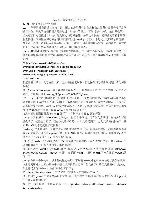
在FLUENT中可用的湍流模型
1-方程模型 - Spalart-Allmaras 2-方程模型 - 标准 k–ε RNG k–ε realizable k–ε 标准 k–ω SST k–ω 雷诺德应力模型 分离涡模拟 大涡模拟
Boussinesq假设 – Reynolds 应力 通过使用涡流粘性(湍流粘性)µT模 拟, 对简单湍流剪切流来说假设是合理的,例如 边界层、 圆形射流 、 混合层、 管流 等等。(S-A, k–ε )
(2) 雷诺德应力模型 (通过雷诺应力输运方程)
RSM 对复杂的 3D湍流流动更有效,但是模型更加复杂, 计算强度 更大, 比涡粘模型更难收敛
方程封闭
RANS 模型能够用下列方法封闭 (1) 涡粘模型 (通过 Boussinesq 假设)
∂ui ∂u j 2 ∂uk 2 − µT Rij = −ρ ui′u′j = µT + δ − ρ k δij ∂x ∂x 3 ∂x ij 3 i k j
RANS 模拟 – 时间平均
将N-S方程中的瞬时变量分解成平均量和脉动量:
1 ui (x, t ) = lim N →∞ N
∑
n =1
N
ui
(n )
(x, t )
ui (x, t )
ui′ (x, t )
ui (x, t )
ui (x, t ) = ui (x, t ) + ui′(x, t )
瞬时项 时均项 波动项
解总体均值(或者时间均值)纳维-斯托克斯方程 在RANS方法中,所有湍流尺度都进行模拟 在工业流动计算中使用得最为广泛
大涡模拟 (LES)
解算空间平均 N-S 方程,大涡直接求解, 比网格尺度小的涡通过模型 得到 计算消耗小于DNS,但是对于大多数的实际应用来说占用计算资源 还是太大了
直接数值模拟 (DNS)
湍流模型
Introductory FLUENT Training
© 2006 ANSYS, Inc. All rights reserved.
ANSYS, Inc. Proprietary
Introductory FLUENT Notes FLUENT v6.3 Augr 2008
Stress production Rotation production Turbulent Dissipation diffusion Pressure Strain
(
)
(
)
Modeling required for these terms
RSM 是最复合物理现象的模型: 各向异性,输运中的雷诺应力可 以直接计算出来 RSM 对控制方程需要更多的建模(其中压应力是最关键和有难度 的参数之一) RSM 比2方程模型需要时间长且较难收敛 适合有大弯曲流线、漩涡和转动的3维流动
流动是否为湍流
外部流动
Re x ≥ 500,000 沿着表面
Re d ≥ 20,000 沿着障碍物
内部流动
where Re L =
ρU L µ L = x, d , d h , etc.
其它因素比如自由流动湍流,,表 面条件,扰动等,在低雷诺数下 可能导致转变为紊流
Re d h ≥ 2,300
自然对流 Ra ≥ 109 Pr
© 2006 ANSYS, Inc. All rights reserved.
6-8
ANSYS, Inc. Proprietary
Introductory FLUENT Notes FLUENT v6.3 Augr 2008
计算湍流粘性
基于量纲分析, µT 能够由 湍流时间尺度 (或速度尺度) 和空间尺 度来决定
每种湍流模型用不同的方法计算 µT
标准 k–ε, RNG k–ε, Realizable k–ε
解关于 k 和 ε的输运方程.
标准 k–ω, SST k–ω
解关于 k 和 ω的输运方程.
© 2006 ANSYS, Inc. All rights reserved.
6-9
ANSYS, Inc. Proprietary
k–ε 湍流模型
标准 k–ε (SKE) 模型
在工程应用中使用最为广泛的湍流模型 稳定而且相对精确 包括可压缩性、 浮力、 燃烧等子模型 局限性