ICLR17论文Do Deep Convolutional Nets Really Need to be Deep and Convolutional
深度学习的目标跟踪算法综述
深度学习的目标跟踪算法综述引言:随着深度学习技术的快速发展,目标跟踪领域也得到了巨大的发展。
目标跟踪是指在视频序列中,对感兴趣的目标进行连续的定位和跟踪,其在计算机视觉、自动驾驶、视频监控等领域有着广泛的应用前景。
本文将综述几种常见的深度学习目标跟踪算法,以便读者对这一领域有更全面的了解。
一、基于卷积神经网络的目标跟踪算法卷积神经网络(Convolutional Neural Network,CNN)是深度学习中最常用的网络结构之一。
它通过卷积层、池化层和全连接层等结构,能够自动提取图像特征。
在目标跟踪中,常用的基于CNN的算法有Siamese网络、Correlation Filter网络和DeepSORT等。
1. Siamese网络Siamese网络是一种基于孪生网络结构的目标跟踪算法,它通过输入一对图像样本来学习两个样本之间的相似度。
该网络通过训练得到的特征向量,可以用于计算待跟踪目标与骨干网络中的目标特征之间的距离,从而确定目标的位置。
2. Correlation Filter网络Correlation Filter网络是一种基于卷积神经网络的目标跟踪算法,它通过训练得到的滤波器,可以将目标与背景进行区分。
该算法通过计算滤波响应图,来确定目标的位置和尺度。
3. DeepSORTDeepSORT是一种结合深度学习和传统目标跟踪算法的方法,它通过使用CNN进行特征提取,并结合卡尔曼滤波器对目标进行预测和更新。
DeepSORT在准确性和实时性上都有较好的表现,在实际应用中有着广泛的使用。
二、基于循环神经网络的目标跟踪算法循环神经网络(Recurrent Neural Network,RNN)是一种能够处理序列数据的神经网络模型。
在目标跟踪中,RNN可以考虑到目标在时间上的依赖关系,从而提高跟踪的准确性。
常见的基于RNN的目标跟踪算法有LSTM和GRU等。
1. LSTMLSTM是一种常用的循环神经网络结构,它能够有效地处理长期依赖问题。
ICLR17论文Adversarial Machine Learning at Scale
1
I NTRODUCn that machine learning models are often vulnerable to adversarial manipulation of their input intended to cause incorrect classification (Dalvi et al., 2004). In particular, neural networks and many other categories of machine learning models are highly vulnerable to attacks based on small modifications of the input to the model at test time (Biggio et al., 2013; Szegedy et al., 2014; Goodfellow et al., 2014; Papernot et al., 2016b). The problem can be summarized as follows. Let’s say there is a machine learning system M and input sample C which we call a clean example. Let’s assume that sample C is correctly classified by the machine learning system, i.e. M (C ) = ytrue . It’s possible to construct an adversarial example A which is perceptually indistinguishable from C but is classified incorrectly, i.e. M (A) = ytrue . These adversarial examples are misclassified far more often than examples that have been perturbed by noise, even if the magnitude of the noise is much larger than the magnitude of the adversarial perturbation (Szegedy et al., 2014). Adversarial examples pose potential security threats for practical machine learning applications. In particular, Szegedy et al. (2014) showed that an adversarial example that was designed to be misclassified by a model M1 is often also misclassified by a model M2 . This adversarial example transferability property means that it is possible to generate adversarial examples and perform a misclassification attack on a machine learning system without access to the underlying model. Papernot et al. (2016a) and Papernot et al. (2016b) demonstrated such attacks in realistic scenarios. It has been shown (Goodfellow et al., 2014; Huang et al., 2015) that injecting adversarial examples into the training set (also called adversarial training) could increase robustness of neural networks to adversarial examples. Another existing approach is to use defensive distillation to train the network (Papernot et al., 2015). However all prior work studies defense measures only on relatively small datasets like MNIST and CIFAR10. Some concurrent work studies attack mechanisms on ImageNet (Rozsa et al., 2016), focusing on the question of how well adversarial examples transfer between different types of models, while we focus on defenses and studying how well different types of adversarial example generation procedures transfer between relatively similar models. 1
计算机视觉论文
计算机视觉论文1000字计算机视觉是指计算机利用图像处理、模式识别、计算几何、人工智能等技术实现对图像的理解与分析,从而使计算机从图片、视频等视觉信息中获取更丰富的信息,并利用这些信息完成人们所需要的各种功能和任务。
下面介绍几篇比较经典的计算机视觉论文。
1. R-CNN: Object Detection via Region-based Convolutional Networks这篇论文由Ross Girshick等人在2014年提出,是深度学习在目标检测领域的开山之作。
该方法将传统的滑动窗口式检测方式替换成针对提取候选区域的局部卷积神经网络(region-based convolutional network, R-CNN)。
此方法首先提取一系列候选框(region proposals),然后将这些框区域输入到卷积神经网络中进行分类和回归。
该模型最终能够实现高准确率的目标检测,同时也大大缩短了计算时间。
2. Deep Residual Learning for Image Recognition这篇论文由Kaiming He等人于2016年提出。
该论文主要研究了深度网络的深度和精度之间的矛盾,并提出了残差学习的思路。
残差学习通过增加跨层连接,将网络的前后输出进行直接相加,从而使得网络学习到不同的特征时不会失去过多原有的信息。
这种方法的应用不仅能够提高深度网络的精度,还能够帮助深度网络降低梯度消失等问题。
3. Generative Adversarial Networks该论文由Ian Goodfellow等人于2014年提出。
这是一种生成式模型,通过在训练过程中,同时训练一个生成器网络并一个判别器网络,从而实现高效的数据生成。
该方法的创新之处在于将生成式模型的随机噪声与判别式模型的决策结合起来,通过互相博弈的方式逐渐提升网络的表现。
该方法不仅能够生成高质量、多样性的样本数据,也可以在图像修复、语音识别等任务中得到广泛应用。
ImageNetClassificationwithDeepConvolutionalNeuralN
ImageNet Classification with Deep Convolutional Neural NetworksAlex Krizhevsky, Ilya Sutskever, Geoffrey E. Hinton摘要咱们训练了一个大型的深度卷积神经网络,来将在ImageNet LSVRC-2020大赛中的120万张高清图像分为1000个不同的类别。
对测试数据,咱们取得了top-1误差率%,和top-5误差率%,那个成效比之前最顶尖的都要好得多。
该神经网络有6000万个参数和650,000个神经元,由五个卷积层,和某些卷积层后随着的max-pooling层,和三个全连接层,还有排在最后的1000-way的softmax层组成。
为了使训练速度更快,咱们利用了非饱和的神经元和一个超级高效的GPU关于卷积运算的工具。
为了减少全连接层的过拟合,咱们采纳了最新开发的正那么化方式,称为“dropout”,它已被证明是超级有效的。
在ILSVRC-2021大赛中,咱们又输入了该模型的一个变体,并依托top-5测试误差率%取得了成功,相较较下,次优项的错误率是%。
1 引言当前物体识别的方式大体上都利用了机械学习方式。
为了改善这些方式的性能,咱们能够搜集更大的数据集,学习更强有力的模型,并利用更好的技术,以避免过拟合。
直到最近,标记图像的数据集都相当小——大约数万张图像(例如,NORB [16],Caltech-101/256 [8, 9],和CIFAR-10/100 [12])。
简单的识别任务能够用这种规模的数据集解决得相当好,专门是当它们用标签-保留转换增强了的时候。
例如,在MNIST数字识别任务中当前最好的误差率(<%)接近于人类的表现[4]。
可是现实环境中的物体表现出相当大的转变,因此要学习它们以对它们进行识别就必需利用更大的训练集。
事实上,小规模图像数据集的缺点已被普遍认同(例如,Pinto等人[21]),可是直到最近,搜集有着上百万张图像的带标签数据集才成为可能。
ICLR17论文Visualizing Deep Neural Network Decisions Prediction Difference Analysis
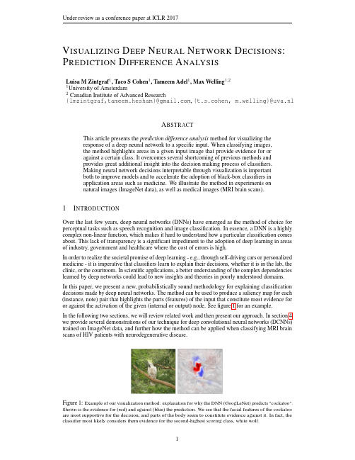
V ISUALIZING D EEP N EURAL N ETWORK D ECISIONS: P REDICTION D IFFERENCE A NALYSISLuisa M Zintgraf1,Taco S Cohen1,Tameem Adel1,Max Welling1,21University of Amsterdam2Canadian Institute of Advanced Research{lmzintgraf,tameem.hesham}@,{t.s.cohen,m.welling}@uva.nlA BSTRACTThis article presents the prediction difference analysis method for visualizing theresponse of a deep neural network to a specific input.When classifying images,the method highlights areas in a given input image that provide evidence for oragainst a certain class.It overcomes several shortcoming of previous methods andprovides great additional insight into the decision making process of classifiers.Making neural network decisions interpretable through visualization is importantboth to improve models and to accelerate the adoption of black-box classifiers inapplication areas such as medicine.We illustrate the method in experiments onnatural images(ImageNet data),as well as medical images(MRI brain scans).1I NTRODUCTIONOver the last few years,deep neural networks(DNNs)have emerged as the method of choice for perceptual tasks such as speech recognition and image classification.In essence,a DNN is a highly complex non-linear function,which makes it hard to understand how a particular classification comes about.This lack of transparency is a significant impediment to the adoption of deep learning in areas of industry,government and healthcare where the cost of errors is high.In order to realize the societal promise of deep learning-e.g.,through self-driving cars or personalized medicine-it is imperative that classifiers learn to explain their decisions,whether it is in the lab,the clinic,or the courtroom.In scientific applications,a better understanding of the complex dependencies learned by deep networks could lead to new insights and theories in poorly understood domains.In this paper,we present a new,probabilistically sound methodology for explaining classification decisions made by deep neural networks.The method can be used to produce a saliency map for each (instance,note)pair that highlights the parts(features)of the input that constitute most evidence for or against the activation of the given(internal or output)node.Seefigure1for an example.In the following two sections,we will review related work and then present our approach.In section4 we provide several demonstrations of our technique for deep convolutional neural networks(DCNNs) trained on ImageNet data,and further how the method can be applied when classifying MRI brain scans of HIV patients with neurodegenerative disease.Figure1:Example of our visualization method:explanation for why the DNN(GoogLeNet)predicts"cockatoo". Shown is the evidence for(red)and against(blue)the prediction.We see that the facial features of the cockatoo are most supportive for the decision,and parts of the body seem to constitute evidence against it.In fact,the classifier most likely considers them evidence for the second-highest scoring class,white wolf.2R ELATED W ORKBroadly speaking,there are two approaches for understanding DCNNs through visualization inves-tigated in the literature:find an input image that maximally activates a given unit or class score to visualize what the network is looking for (Erhan et al.,2009;Simonyan et al.,2013;Yosinski et al.,2015),or visualize how the network responds to a specific input image in order to explain a particular classification made by the network.The latter will be the subject of this paper.One such instance-specific method is class saliency visualization proposed by Simonyan et al.(2013)who measure how sensitive the classification score is to small changes in pixel values,by computing the partial derivative of the class score with respect to the input features using standard backpropagation.They also show that there is a close connection to using deconvolutional networks for visualization,proposed by Zeiler &Fergus (2014).Other methods include Shrikumar et al.(2016),who compare the activation of a unit when a specific input is feed forward through the net to a reference activation for that unit.Zhou et al.(2016)and Bach et al.(2015)also generate interesting visualization results for individual inputs,but are both not as closely related to our method as the two papers mentioned above.The idea of our method is similar to an analysis Zeiler &Fergus (2014)make:they estimate the importance of input pixels by visualizing the probability of the (correct)class as a function of a gray patch occluding parts of the image.In this paper,we will take a more rigorous approach at both removing information from the image and evaluating the effect of this.In the field of medical image classification specifically,a widely used method for visualizing feature importances is to simply plot the weights of a linear classifier (Klöppel et al.,2008;Ecker et al.,2010),or the p-values of these weights (determined by permutation testing)(Mourao-Miranda et al.,2005;Wang et al.,2007).These are independent of the input image,and,as argued by Gaonkar &Davatzikos (2013)and Haufe et al.(2014),interpreting these weights can be misleading in general.The work presented in this paper is based on an instance-specific method by Robnik-Šikonja &Kononenko (2008),the prediction difference analysis ,which is reviewed in the next section.Our main contributions are three substantial improvements of this method:conditional sampling (section3.1),multivariate analysis (section 3.2),and deep visualization (section 3.3).3A PPROACHOur method is based on the technique presented by Robnik-Šikonja &Kononenko (2008),which we will now review.For a given prediction,the method assigns a relevance value to each input feature with respect to a class c .The basic idea is that the relevance of a feature x i can be estimated by measuring how the prediction changes if the feature is unknown,i.e.,the difference between p (c |x )and p (c |x \i ),where x \i denotes the set of all input features except x i .To find p (c |x \i ),i.e.,evaluate the prediction when a feature is unknown,the authors propose three strategies.The first is to label the feature as unknown (which only few classifiers allow).The second is to re-train the classifier with the feature left out (which is clearly infeasible for DNNs and high-dimensional data like images).The third approach is to simulate the absence of a feature by marginalizing the feature:p (c |x \i )= x ip (x i |x \i )p (c |x \i ,x i )(1)(with the sum running over all possible values for x i ).However,modeling p (x i |x \i )can easily become infeasible with a large number of features.Therefore,the authors approximate equation 1by assuming that feature x i is independent of the other features,x \i :p (c |x \i )≈ x ip (x i )p (c |x \i ,x i ).(2)The prior probability p (x i )is usually approximated by the empirical distribution for that feature.Once the class probability p (c |x \i )is estimated,it can be compared to p (c |x ).We will stick to an evaluation proposed by the authors referred to as weight of evidence ,given by WE i (c |x )=log 2(odds (c |x ))−log 2 odds (c |x \i ) ,(3)Figure2:Simple illustration of the sampling procedure in algorithm1.Given the input image x,we select every possible patch x w(in a sliding window fashion)of size k×k and place a larger patchˆx w of size l×l around it.We can then conditionally sample x w by conditioning on the surrounding patchˆx w.Algorithm1Evaluating the prediction difference using conditional and multivariate sampling class of interest c,probabilistic model over patches of size l×l,number of samples S Initialization:WE=zeros(n*n),counts=zeros(n*n)for every patch x w of size k×k in x dox =copy(x)sum w=0define patchˆx w of size l×l that contains x wfor s=1to S dox w←x w sampled from p(x w|ˆx w\x w)sum w+=p(c|x ) evaluate classifier end forp(c|x\x w):=sum w/SWE[coordinates of x w]+=log2(odds(c|x))−log2(odds(c|x\x w))counts[coordinates of x w]+=1end forOutput:WE/counts point-wise division where odds(c|x)=p(c|x)/(1−p(c|x)).To avoid problems with zero probabilities,Laplace correction p←(pN+1)/(N+K)is used,where N is the number of training instances and K the number of classes.The method produces a relevance vector(WE i)i=1...m(m being the number of features)of the same size as the input,which reflects the relative importance of all features.A large prediction difference means that the feature contributed substantially to the classification,whereas a small difference indicates that the feature was not important for the decision.A positive value WE i means that the feature has contributed evidence for the class of interest:removing it would decrease the confidence of the classifier in the given class.A negative value on the other hand indicates that the feature displays evidence against the class:removing it also removes potentially conflicting or irritating information and the classifier becomes more certain in the investigated class.3.1C ONDITIONAL S AMPLINGIn equation(3),the conditional probability p(x i|x\i)of a feature x i is approximated using the marginal distribution p(x i).This is a very crude approximation.In images for example,a pixel’s value is highly dependent on other pixels.We propose a much more accurate approximation,based on the following two observations:a pixel depends most strongly on a small neighborhood around it, and the conditional of a pixel given its neighborhood does not depend on the position of the pixel in the image.For a pixel x i,we can thereforefind a patchˆx i of size l×l that contains x i,and condition on the remaining pixels in that patch:p(x i|x\i)≈p(x i|ˆx\i).(4) This greatly improves the approximation while remaining completely tractable.For a feature to become relevant when using conditional sampling,it now has to satisfy two conditions: being relevant to predict the class of interest,and be hard to predict from the neighboring pixels. Relative to the marginal method,we therefore downweight the pixels that can easily be predicted and are thus redundant in this sense.3.2M ULTIVARIATE A NALYSISRobnik-Šikonja&Kononenko(2008)take a univariate approach:only one feature at a time is removed.However,we would expect that a neural network is relatively robust to just one feature of a high-dimensional input being unknown,like a pixel in an image.Therefore,we will remove several features at once by again making use of our knowledge about images by strategically choosing these feature sets:patches of connected pixels.Instead of going through all individual pixels,we go through all patches of size k×k in the image(k×k×3for RGB images and k×k×k for3D images like MRI scans),implemented in a sliding window fashion.The patches are overlapping,so that ultimately an individual pixel’s relevance is obtained by taking the average relevance obtained from the different patches it was in.Algorithm1andfigure2illustrate how the method can be implemented,incorporating the proposed improvements.3.3D EEP V ISUALIZATION OF H IDDEN L AYERSWhen trying to understand neural networks and how they make decisions,it is not only interesting to analyze the input-output relation of the classifier,but also to look at what is going on inside the hidden layers of the network.We can adapt the method to see how the units of any layer of the network influence a node from a deeper layer.Mathematically,we can formulate this as follows.Let h be the vector representation of the values in a layer H in the network(after forward-propagating the input up to this layer).Further,let z=z(h)be the value of a node that depends on h,i.e.,a node in a subsequent layer.Then the analog of equation(2)is given by the expectation:g(z|h\i)≡E p(hi |h\i)[z(h)]=h ip(h i|h\i)z(h\i,h i),(5)which expresses the distribution of z when unit h i in layer H is unobserved.The equation now works for arbitrary layer/unit combinations,and evaluates to the same as equation(1)when the input-output relation is analyzed.To evaluate the difference between g(z|h)and g(z|h\i),we will in general use the activation difference,AD i(z|h)=g(z|h)−g(z|h\i),for the case when we are not dealing with probabilities(and equation3is not applicable).4E XPERIMENTSIn this section,we illustrate how the proposed visualization method can be applied,on the ImageNet dataset of natural images when using DCNNs(section4.1),and on a medical imaging dataset of MRI scans when using a logistic regression classifier(section4.2).For marginal sampling we always use the empirical distribution,i.e.,we replace a feature(patch)with samples taken directly from other images,at the same location.For conditional sampling we use a multivariate normal distribution.For both sampling methods we use10samples to estimate p(c|x\i)(since no significant difference was observed with more samples).Note that all images are best viewed digital and in color.Our implementation is available at /lmzintgraf/DeepVis-PredDiff.4.1I MAGE N ET:U NDERSTANDING HOW A DCNN MAKES DECISIONSWe use images from the ILSVRC challenge Russakovsky et al.(2015)(a large dataset of natural im-ages from1000categories)and three DCNNs:the AlexNet(Krizhevsky et al.,2012),the GoogLeNet (Szegedy et al.,2015)and the(16-layer)VGG network(Simonyan&Zisserman,2014).We used the publicly available pre-trained models that were implemented using the deep learning framework caffe (Jia et al.,2014).Analyzing one image took us on average20,30and70minutes for the respective classifiers AlexNet,GoogLeNet and VGG(using the GPU implementation of caffe and mini-batches with the standard settings of10samples and a window size of10).The results shown here are chosen from among a small set of images in order to show a range of behavior of the algorithm.The shown images are quite representative of the performance of the method in general.Examples on randomly selected images,including a comparison to the sensitivity analysis of Simonyan et al.(2013),can be seen in appendix A.Figure3:Visualization of the effects of marginal versus conditional sampling using the GoogLeNet classifier.The classifier makes correct predictions(ostrich and saxophone),and we show the evidence for(red) and against(blue)this decision at the output layer.We can see that conditional sampling gives more targeted explanations compared to marginal sampling.Also,marginal sampling assigns too much importance on pixels that are easily predictable conditioned on their neighboring pixels.Figure4:Visualization of how different window sizes influence the visualization result.We used the conditional sampling method and the AlexNet classifier with l=k+4and varying k.We can see that even when removing single pixels(k=1),this has a noticeable effect on the classifier and more important pixels get a higher score.By increasing the window size we can get a more easily interpretable,smooth result until the image gets blurry for very large window sizes.We start this section by demonstrating our proposed improvements(sections3.1-3.3).Marginal vs Conditional SamplingFigure3shows visualizations of the spatial support for the highest scoring class,using marginal and conditional sampling(with k=10and l=14).We can see that conditional sampling leads to results that are more refined in the sense that they concentrate more around the object.We can also see that marginal sampling leads to pixels being declared as important that are very easily predictable conditioned on their neighboring pixels(like in the saxophone example).Throughout our experiments, we have found that conditional sampling tends to give more specific andfine-grained results than marginal sampling.For the rest of our experiments,we will therefore show results using conditional sampling only.Multivariate AnalysisFor ImageNet data,we have observed that setting k=10gives a good trade-off between sharp results and a smooth appearance.Figure4shows how different window sizes influence the resolution of the visualization.Surprisingly,removing only one pixel does have a measurable effect on the prediction, and the largest effect comes from sensitive pixels.We expected that removing only one pixel does not have any effect on the classification outcome,but apparently the classifier is sensitive even to these small changes.However when using such a small window size,it is difficult to make sense of the sign information in the visualization.If we want to get a good impression of which parts in the image are evidence for/against a class,it is therefore better to use larger windows.If k is chosen too large however,the results tend to get blurry.Note that these results are not just simple averages of one another,but a multivariate approach is indeed necessary to observe the presented results. Deep Visualization of Hidden Network LayersOur third main contribution was the extension of the method to neural networks;to understand the role of hidden layers in a DNN.Figure5shows how different feature maps in three different layers of the GoogLeNet react to the input of a tabby cat(seefigure6,middle image).For each feature map in a convolutional layer,wefirst compute the relevance of the input image for each hidden unit in that map.To estimate what the feature map as a whole is doing,we show the average of the relevance vectors over all units in that feature map.Thefirst convolutional layer works with different types of simple imagefilters(e.g.,edge detectors),and what we see is which parts of the input image respondFigure5:Visualization of feature maps from thee different layers of the GoogLeNet(l.t.r.:”conv1/7x7_s2”,”inception_3a/output”,”inception_5b/output”),using conditional sampling and patch sizes k=10and l=14 (see alg.1).For each feature map in the convolutional layer,wefirst evaluate the relevance for every single unit, and then average the results over all the units in one feature map to get a sense of what the unit is doing as a whole.Red pixels activate a unit,blue pixels decreased the activation.Figure6:Visualization of three different feature maps,taken from the”inception_3a/output”layer of the GoogLeNet(from the middle of the network).Shown is the average relevance of the input features over all activations of the feature map.We used patch sizes k=10and l=14(see alg.1).Red pixels activate a unit, blue pixels decreased the activation.positively or negatively to thesefilters.The layer we picked from somewhere in the middle of the network is specialized to higher level features(like facial features of the cat).The activations of the last convolutional layer are very sparse across feature channels,indicating that these units are highly specialized.To get a sense of what single feature maps in convolutional layers are doing,we can look at their visualization for different input images and search for patterns in their behavior.Figure6shows this for four different feature maps from a layer from the middle of the GoogLeNet network.Here,we can directly see which kind of features the model has learned at this stage in the network.For example, one feature map is activated by the eyes of animals(third row),and another is looking mostly at the background(last row).Penultimate vs Output LayerIf we visualize the influence of the input features on the penultimate(pre-softmax)layer,we show only the evidence for/against this particular class,without taking other classes into consideration. After the softmax operation however,the values of the nodes are all interdependent:a drop in the probability for one class could be due to less evidence for it,or because a different class becomes more likely.Figure7compares visualizations for the last two layers.By looking at the top three scoring classes,we can see that the visualizations in the penultimate layer look very similar if the classes are similar(like different dog breeds).When looking at the output layer however,they look rather different.Consider the case of the elephants:the top three classes are different elephant subspecies,and the visualizations of the penultimate layer look similar since every subspecies can be identified by similar characteristics.But in the output layer,we can see how the classifier decides for one of the three types of elephants and against the others:the ears in this case are the crucial difference.Figure7:Visualization of the support for the top-three scoring classes in the penultimate-and output layer.Next to the input image,thefirst row shows the results with respect to the penultimate layer;the second row with respect to the output layer.For each image,we additionally report the values of the units.We used the AlexNet with conditional sampling and patch sizes k=10and l=14(see alg.1).Red pixels are evidence for-,blue against a class.Figure8:Comparison of the prediction visualization of different NN architectures.For two input images, we show the results of the prediction difference analysis when using different neural networks-(f.l.t.r.)the AlexNet,GoogLeNet and VGG network.Network ComparisonWhen analyzing how neural networks make decisions,we can also compare how different network architectures influence the visualization.Here,we tested our method on the AlexNet,the GoogLeNet and the VGG network.Figure8shows the results for the three different networks,on two input images.The AlexNet seems to more on contextual information(the sky in the balloon image), which could be attributed to it having the least complex architecture compared to the other two networks.It is also interesting to see that the VGG network deems the basket of the balloon as very important compared to all other pixels.The second highest scoring class in this case was a parachute -presumably,the network learned to not confuse a balloon with a parachute by detecting a square basket(and not a human).4.2MRI DATA:E XPLAINING C LASSIFIER D ECISIONS IN M EDICAL I MAGINGTo show how our visualization method can also be useful in a medical domain,we show some experimental results on an MRI dataset of HIV and healthy patients.In such settings,it is crucial that the practitioner has some insight into the algorithm’s decision when classifying a patient,to weigh this information and incorporate it in the overall diagnosis process.The dataset used here is referred to as the COBRA dataset.It contains3D MRIs from100HIV patients and70healthy individuals,included in the Academic Medical Center(AMC)in Amsterdam, The Netherlands.Of these subjects,diffusion weighted MRI data were acquired.Preprocessing of the data was performed with software developed in-house,using the HPCN-UvA Neuroscience Gateway and using resources of the Dutch e-Science Grid Shahand et al.(2015).As a result,Fractional Anisotropy(FA)maps were computed.FA is sensitive to microstructural damage and therefore expected to be,on average,decreased in patients.Subjects were scanned on two3.0Tesla scanner systems,121subjects on a Philips Intera system and39on a Philips Ingenia system.Patients and controls were evenly distributed.FA images were spatially normalized to standard space Anderssonet al.(2007),resulting in volumes with91×109×91=902,629voxels.We trained an L2-regularized Logistic Regression classifier on a subset of the MRI slices(slices 29-40along thefirst axis)and on a balanced version of the dataset(by taking thefirst70samples of the HIV class)to achieve an accuracy of69.3%in a10-fold cross-validation test.Analyzing one image took around half an hour(on a CPU,with k=3and l=7,see algorithm1).For conditional sampling,we also tried adding location information in equation(2),i.e.,we split up the3D image into a20×20×20grid and also condition on the index in that grid.We found that this slightly improved the interpretability of the results,since the pixel values in the special case of MRI scans does depend on spacial location as well.Figure9(first row)shows one way via which the prediction difference results could be presented to a physician,for an HIV sample.By overlapping the prediction difference and the MRI image, the exact regions can be pointed out that are evidence for(red parts)or against(blue parts)the classifier’s decision.The second row shows the results using the weights of the logistic regression classifier,which is a commonly used method in neuroscientific literature.We can see that they are considerably noisier(in the sense that,compared to our method,the voxels relevant for the classification decisions are more scattered),and also,they are not specific to the given image.Figure 10shows the visualization results for four healthy-,and four HIV samples.We can clearly see that the patterns for the two classes are distinct,and there is some pattern to the decision of the classifier, but which is still specific to the input image.In clinical practice,a3D animation where different slices and window sizes can be adjusted can be very useful for analyzing the visualization result. Figure11shows the same(HIV)sample as infigure9along different axes,andfigure12shows how the visualization changes with different patch sizes.We believe that both varying the slice and patch size can give different insights to a clinician,and a3D animation with variable parameters could be very useful in practice.In general we can assume that the better the classifier,the closer the explanations for its decisions are to the true class difference.For clinical practice it is therefore crucial to have very good classifiers. This will increase computation time,but in many medical settings,longer waiting times for test results are common and worth the wait if the patient is not in an acute life threatening condition(e.g., when predicting HIV or Alzheimer from MRI scans,or thefield of cancer diagnosis and detection). The presented results here are for demonstration purposes of the visualization method,and a thorough qualitative analysis incorporating expert knowledge is outside the scope of this paper.5F UTURE WORKIn our experiments,we used a simple multivariate normal distribution for conditional sampling.We can imagine that using more sophisticated generative models will lead to better results:pixels that are easily predictable by their surrounding are downweighted even more.However this will also significantly increase the computational resources needed to produce the explanations.Similarly, we could try to modify equation(4)to get an even better approximation by using a conditional distribution that takes more information about the whole image into account(like adding spatial information for the MRI scans).To make the method applicable for clinical analysis and practice,a better classification algorithm is required.Also,software that visualizes the results as an interactive3D model will improve the usability of the system.6C ONCLUSIONWe have presented a new method for visualizing deep neural networks that improves on previous methods by using a more powerful conditional,multivariate model.The visualization method shows which pixels of a specific input image are evidence for or against a node in the network.The signed information offers new insights-for research on the networks,as well as the acceptance and usability in domains like healthcare.While our method requires significant computational resources,real-time 3D visualization is possible when visualizations are pre-computed.With further optimization and powerful GPUs,pre-computation time can be reduced a lot further.In our experiments,we have presented several ways in which the visualization method can be put into use for analyzing how DCNNs make decisions.Figure9:Visualization of the support for the correct classification”HIV”,using the Prediction Differ-ence method and Logistic Regression Weights.For an HIV sample,we show the results with the prediction difference(first row),and using the weights of the logistic regression classifier(second row),for slices29and 40(along thefirst axis).Red are positive values,and blue negative.For each slice,the left image shows the the original image,overlaid with the relevance values.The right image shows the original image with reversed colors and the relevance values.All voxels with(absolute)relevance value above of15%of the(absolute)maximum value are shown.Figure10:Prediction Difference visualization for different samples.Thefirst four samples are of the class ’Healthy’,and the last four of the class”HIV”.All images show slice39(along thefirst axis).All samples are correctly classified,and the results show evidence for(red)and against(blue)this decision.All voxels with(absolute)value above of15%of the(absolute)maximum value are shown for the prediction difference.Figure11:Visualization results across different slices of the MRI image,using the same input image as shown in9.All voxels with(absolute)value above of15%of the(absolute)maximum value are shown for theprediction difference.Figure12:How the patch size influences the visualization.For the input image(HIV sample,slice39along thefirst axis)we show the visualization with different patch sizes(k in alg.1).All voxels with(absolute)valueabove of15%of the(absolute)maximum value are shown for the prediction difference(for k=2it is10%)。
神经网络 论文

神经网络论文以下是一些关于神经网络的重要论文:1. "A Computational Approach to Edge Detection",作者:John Canny,论文发表于1986年,提出了一种基于神经网络的边缘检测算法,被广泛应用于计算机视觉领域。
2. "Backpropagation Applied to Handwritten Zip Code Recognition",作者:Yann LeCun et al.,论文发表于1990年,引入了反向传播算法在手写数字识别中的应用,为图像识别领域开创了先河。
3. "Gradient-Based Learning Applied to Document Recognition",作者:Yann LeCun et al.,论文发表于1998年,介绍了LeNet-5,一个用于手写数字和字符识别的深度卷积神经网络。
4. "ImageNet Classification with Deep Convolutional Neural Networks",作者:Alex Krizhevsky et al.,论文发表于2012年,提出了深度卷积神经网络模型(AlexNet),在ImageNet图像识别竞赛中取得了重大突破。
5. "Deep Residual Learning for Image Recognition",作者:Kaiming He et al.,论文发表于2015年,提出了深度残差网络(ResNet),通过引入残差连接解决了深度神经网络训练中的梯度消失和梯度爆炸问题。
6. "Generative Adversarial Networks",作者:Ian Goodfellow etal.,论文发表于2014年,引入了生成对抗网络(GAN),这是一种通过博弈论思想训练生成模型和判别模型的框架,广泛应用于图像生成和增强现实等领域。
算法论文范文
算法论文范文摘要本文介绍了一种基于深度学习的图像分类算法。
该算法采用卷积神经网络(CNN)作为特征提取器,并结合支持向量机(SVM)进行分类。
实验结果表明,该算法在多个数据集上均取得了优秀的分类效果。
引言图像分类是计算机视觉领域的一个重要问题。
在实际应用中,我们需要将大量的图像按照其所属的类别进行分类。
传统的图像分类方法通常采用手工设计的特征提取器,如SIFT、HOG等。
这些方法虽然在一定程度上能够提取出图像的特征,但是其性能受到了很多限制,如对光照、旋转、尺度等变化的敏感性。
近年来,深度学习技术的发展为图像分类带来了新的思路。
卷积神经网络(CNN)是一种基于深度学习的图像分类方法,其可以自动学习图像的特征,并且对于光照、旋转、尺度等变化具有较好的鲁棒性。
本文提出了一种基于CNN的图像分类算法,并结合支持向量机(SVM)进行分类。
算法描述数据预处理在进行图像分类之前,我们需要对数据进行预处理。
本文采用了CIFAR-10数据集进行实验,该数据集包含了10个类别的60000张32x32的彩色图像。
我们首先将图像进行归一化处理,将像素值缩放到[0,1]之间。
然后,我们将数据集分为训练集和测试集,其中训练集包含50000张图像,测试集包含10000张图像。
特征提取本文采用了一个5层的卷积神经网络(CNN)作为特征提取器。
该网络的结构如下所示:Convolutional layer (32 filters, 3x3 kernel, stride 1)ReLU activationMax pooling layer (2x2 kernel, stride 2)Convolutional layer (64 filters, 3x3 kernel, stride 1)ReLU activationMax pooling layer (2x2 kernel, stride 2)Convolutional layer (128 filters, 3x3 kernel, stride 1)ReLU activationMax pooling layer (2x2 kernel, stride 2)Fully connected layer (1024 units)ReLU activation在训练过程中,我们采用了随机梯度下降(SGD)算法进行优化。
高被引论文
高被引论文以下是一些高被引论文的例子:1. "Deep Residual Learning for Image Recognition" - 这篇论文由何凯明等人于2016年发表在IEEE Conference on Computer Vision and Pattern Recognition (CVPR)会议上。
它介绍了一种用于图像识别的深度残差学习方法,该方法在图像分类、检测和分割等任务上均取得了显著的性能提升。
2. "Attention is All You Need" - 这篇论文由Vaswani等人于2017年发表在NeurIPS会议上。
它引入了一种名为Transformer的神经网络架构,该架构通过自注意力机制实现了端到端的序列到序列的模型,取得了在机器翻译等任务上优异的结果。
3. "Generative Adversarial Networks" - 这篇论文由Goodfellow 等人于2014年发表在NeurIPS会议上。
它提出了一种新颖的生成模型架构,即生成对抗网络(GANs),该架构通过竞争式学习的方式同时训练生成器和判别器模型,取得了在图像生成和样式迁移等领域的突破性进展。
4. "The Unreasonable Effectiveness of Deep Learning in Artificial Intelligence" - 这篇论文由LeCun等人于2015年发表在IEEE Conference on Computer Vision and Pattern Recognition (CVPR)会议上。
它综述了深度学习在人工智能领域的应用,阐述了深度学习方法在计算机视觉、语音识别、自然语言处理等任务上的优秀表现。
5. "A Neural Algorithm of Artistic Style" - 这篇论文由Gatys等人于2015年发表在Journal of Vision上。
深度学习论文翻译解析(六):MobileNets:EfficientConvolution。。。
深度学习论⽂翻译解析(六):MobileNets:EfficientConvolution。
论⽂标题:MobileNets:Efficient Convolutional Neural Networks for Mobile Vision Appliications论⽂作者:Andrew G.Howard Menglong Zhu Bo Chen .....代码地址:声明:⼩编翻译论⽂仅为学习,如有侵权请联系⼩编删除博⽂,谢谢!⼩编是⼀个机器学习初学者,打算认真学习论⽂,但是英⽂⽔平有限,所以论⽂翻译中⽤到了Google,并⾃⼰逐句检查过,但还是会有显得晦涩的地⽅,如有语法/专业名词翻译错误,还请见谅,并欢迎及时指出。
如果需要⼩编其他论⽂翻译,请移步⼩编的GitHub地址 传送门:摘要 我们提出⼀个在移动端和嵌⼊式应⽤⾼效的分类模型叫做MobileNets,MobileNets基于流线型架构(streamlined),使⽤深度可分类卷积(depthwise separable convolutions,即Xception 变体结构)来构建轻量级深度神经⽹络。
我们介绍两个简单的全局超参数,可有效的在延迟和准确率之间做折中。
这些超参数允许我们依据约束条件选择合适⼤⼩的模型。
论⽂测试在多个参数量下做了⼴泛的实验,并在ImageNet分类任务上与其他先进模型做了对⽐,显⽰了强⼤的性能。
论⽂验证了模型在其他领域(对象检测,⼈脸识别,⼤规模地理定位等)使⽤的有效性。
1,引⾔ ⾃从AlexNet [19]通过赢得ImageNet挑战:ILSVRC 2012 [24]来推⼴深度卷积神经⽹络以来,卷积神经⽹络就已经在计算机视觉中变得⽆处不在。
总的趋势是建⽴更深,更复杂的⽹络以实现更⾼的准确性[27、31、29、8]。
但是,这些提⾼准确性的进步并不⼀定会使⽹络在⼤⼩和速度⽅⾯更加⾼效。
在许多现实世界的应⽤程序中,例如机器⼈技术,⾃动驾驶汽车和增强现实,识别任务需要在计算受限的平台上及时执⾏。
VeryDeepConvolutionalNetworksforLarge-ScaleIm。。。

VeryDeepConvolutionalNetworksforLarge-ScaleIm。
Very Deep Convolutional Networks for Large-Scale Image Recognition这篇论⽂是今年9⽉份的论⽂[1],⽐較新,当中的观点感觉对卷积神经⽹络的參数调整⼤有指导作⽤,特总结之。
关于卷积神经⽹络(Convolutional Neural Network, CNN),笔者后会作⽂阐述之,读者若⼼急则或可⽤⾕歌百度⼀下。
本⽂下⾯内容即是论⽂的笔记,笔者初次尝试对⼀篇论⽂提取重点做笔记,若有不⾜之处请阅读原⽂者指出。
1. Main Contribution考察在參数总数基本不变的情况下,CNN随着层数的添加,其效果的变化。
论⽂中的⽅法在ILSVRC-2014⽐赛中获得第⼆名。
ILSVRC——ImageNet Large-Scale Visual Recongnition Challenge2. CNN improvement在论⽂[2]出现以后,有⾮常多对其提出的CNN结构进⾏改进的⽅法。
⽐如:Use smaller receptive window size and smaller stride of the first convolutional layer.Training and testing the networks densely over the whole image and over multiple scales.3. CNN Configuration PrincipalsCNN的输⼊都是224×224×3的图⽚。
输⼊前唯⼀的预处理是减去均值。
1×1的核能够被看成是输⼊通道的线性变换。
使⽤较多的卷积核⼤⼩为3×3。
Max-Pooling ⼀般在2×2的像素窗体上做,with stride 2。
深度学习 论文
深度学习论文以下是一些关于深度学习的重要论文:1. Hinton, G. E., Deng, L., Yu, D., Dahl, G. E., Mohamed, A. R., Jaitly, N., ... & Kingsbury, B. (2012). Deep neural networks for acoustic modeling in speech recognition. IEEE signal processing magazine, 29(6), 82-97. 这篇论文介绍了深度神经网络在语音识别中的应用,并实现了显著的性能提升。
2. Krizhevsky, A., Sutskever, I., & Hinton, G. E. (2012). Imagenet classification with deep convolutional neural networks. In Advances in neural information processing systems (pp. 1097-1105). 这篇论文提出并描述了深度卷积神经网络(CNN)在图像分类任务中实现领先结果的方法,为深度学习的图像处理领域开辟了道路。
3. Szegedy, C., Liu, W., Jia, Y., Sermanet, P., Reed, S., Anguelov,D., ... & Rabinovich, A. (2015). Going deeper with convolutions. In Proceedings of the IEEE conference on computer vision and pattern recognition (pp. 1-9). 这篇论文介绍了GoogleNet,一个更深的卷积神经网络结构,在图像分类和目标检测等任务上取得了较好的性能。
深度学习文字识别论文综述

深度学习文字识别论文综述深度学习文字识别论文综述深度学习是机器学习研究中的一个新的领域,其动机在于建立、模拟人脑进行分析学习的神经网络,它模仿人脑的机制来解释数据,例如图像,声音和文本。
深度学习是无监督学习的一种,深度学习采用了神经网络的分层结构,系统包括输入层、隐层(多层)、输出层组成的多层网络,只有相邻的节点之间有连接,同一层以及跨层节点之间相互无连接。
深度学习通过建立类似于人脑的分层模型结构,对输入数据逐级提取从底层到高层的特征,从而能很好地建立从底层信号到高层语义的映射关系。
近年来,谷歌、微软、百度等拥有大数据的高科技公司相继投入大量资源进行深度学习技术研发,在语音、图像、自然语言、在线广告等领域取得显著进展。
从对实际应用的贡献来说,深度学习可能是机器学习领域最近这十年来最成功的研究方向。
深度学习模型不仅大幅提高了图像识别的精度,同时也避免了需要消耗大量的时间进行人工特征提取的工作,使得在线运算效率大大提升。
深度学习用于文字定位论文Thai Text Localization in Natural Scene Images using Convolutional Neural Network主要采用CNN的方法进行自然场景中的文本分类,并根据泰字的特点进行分类后的后处理,得到更加精确的定位效果。
如图1所示为CNN网络模型,CNN网络由一个输入层,两个卷积层和两个下采样层以及一个全连接层组成,输出为一个二分类向量,即文本和非文本。
图1 CNN网络模型该文主要思路为将图像切块后进行训练,采用人工标注样本的方法,使得网络具有识别文本和非文本的能力。
由于样本数量较少,文中采用了根据已有字体生成训练数据集的方法,包括对字体随机添加背景、调整字体风格以及应用滤波器。
如图2为生成的泰字样本,文中在标签的过程中将半个字或者整个字都标记为文本,增加了网络对文字的识别率。
图2训练样本集在使用生成好的网络进行文字定位的过程中,论文采用的编组方法结合了泰字的特点,如图3为对图像文字的初步定位,其中被标记的区域被网络识别为文字。
卷积神经网络论文

卷积神经网络论文引言卷积神经网络(Convolutional Neural Networks,CNN)是一种深度学习算法,广泛应用于图像识别、目标检测、语音识别等领域。
本文旨在介绍CNN的基本原理、网络结构以及应用领域。
CNN的基本原理CNN是一种受到生物视觉启发的神经网络结构,其核心思想是通过卷积操作和池化操作来提取图像的特征。
具体而言,CNN使用一个或多个卷积层来捕获图像中的空间特征,并通过池化层将特征降采样。
此外,CNN还包括全连接层和激活函数来完成分类任务。
卷积层是CNN的关键组成部分,其通过卷积操作将输入特征图与卷积核进行逐元素乘法和求和操作,得到输出特征图。
卷积操作具有局部感受野和权值共享的特点,能够有效地提取图像的局部特征。
池化层用于降低特征图的空间分辨率,通过取区域内的最大值或均值来减少特征数量,从而降低计算复杂度并增加网络的不变性。
全连接层将卷积层和池化层提取的特征映射进行分类,每个神经元都与上一层的所有神经元相连接。
激活函数则引入非线性变换,提高网络的表达能力。
CNN的网络结构CNN的网络结构通常包括卷积层、池化层、全连接层和激活函数。
具体的网络结构可以根据任务需求进行设计和调整。
卷积层卷积层是CNN的核心组成部分,由多个卷积核组成。
每个卷积核通过卷积操作对输入特征图进行处理,生成输出特征图。
卷积核的数量决定了输出特征图的深度。
池化层池化层通过降采样操作减少特征图的尺寸,进一步减少网络的计算复杂度。
常见的池化操作有最大池化和平均池化。
池化层通常与卷积层交替使用。
全连接层全连接层将卷积层和池化层提取的特征映射进行分类。
每个神经元都与上一层的所有神经元相连接,通过权重和偏置实现特征的线性组合和非线性变换。
激活函数激活函数引入非线性变换,提高网络的表达能力。
常见的激活函数有ReLU、Sigmoid和Tanh等。
CNN的应用领域CNN在图像识别、目标检测、语音识别等领域取得了显著的成绩。
基于卷积神经网络的遥感图像识别研究

基于卷积神经网络的遥感图像识别研究近年来,随着遥感技术的不断发展和普及,遥感图像的应用领域不断扩大。
然而,由于遥感图像的高分辨率、多光谱以及大规模等特点,传统的图像处理方法往往难以满足对遥感图像进行准确快速地识别和分类的需求。
而卷积神经网络(Convolutional Neural Network,CNN)在图像识别领域取得了显著的成功,因此,将卷积神经网络应用于遥感图像识别成为当前研究的热点之一。
首先,我们需要对卷积神经网络进行简要介绍。
卷积神经网络是一种深度学习技术,其主要特点是对图像进行卷积运算和池化操作,在网络中逐层进行特征提取和抽象,并通过全连接层进行分类或回归。
卷积神经网络具有参数共享、局部感知以及自动学习等优势,特别适用于图像处理任务。
在遥感图像识别领域,卷积神经网络可以通过学习遥感图像的特征表示,从而实现准确的分类与识别。
其中,卷积层和池化层是卷积神经网络的核心组成部分。
卷积层通过卷积核对输入特征图进行卷积操作,以提取图像的局部特征。
池化层则通过降采样的方式减小特征图的尺寸,从而提高计算效率和网络的鲁棒性。
通过多层卷积层和池化层的迭代,卷积神经网络可以逐渐实现对遥感图像更高层次、更抽象的特征提取与表示。
在遥感图像识别研究中,不同层次的卷积神经网络模型已经被证明有效。
例如,最早提出的LeNet模型主要用于手写数字识别,其包含多个卷积层和池化层,可以对二维图像进行特征提取和分类。
而AlexNet模型则是在大规模图像分类竞赛ImageNet中取得突破性成果的模型,其具有更深的网络结构和更多的卷积核数。
此外,VGG模型、GoogLeNet模型和ResNet模型等也在遥感图像分类中取得了不错的效果。
除了模型的选择外,遥感图像识别研究中还需要考虑数据集的选择和预处理。
由于遥感图像数据量庞大,且存在许多种类和地域差异,合理选择和处理数据集对于提高识别准确率非常重要。
通常,研究者可以选择公开的遥感图像数据集,例如国内外的遥感卫星数据集,或根据具体研究需求自行采集和标注数据。
基于深度卷积网络的阿尔茨海默病诊断模型研究
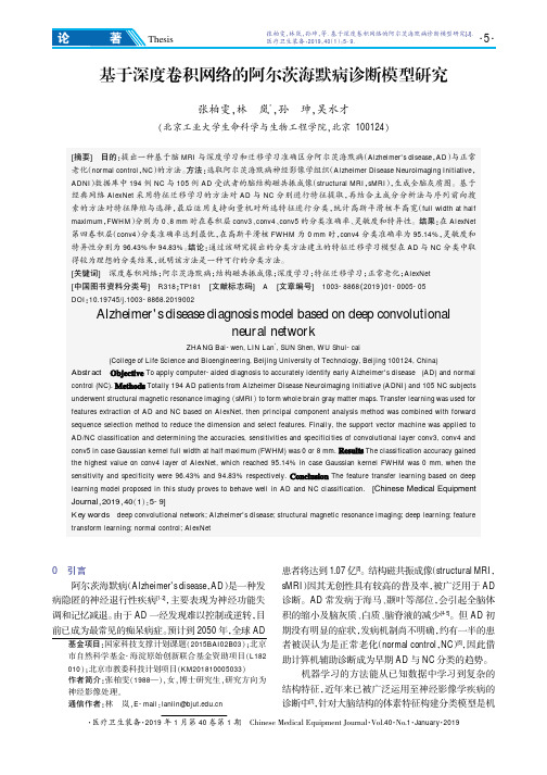
features extraction of AD and NC based on AlexNet, then principal component analysis method was combined with forward
sequence selection method to reduce the dimension and select features. Finally, the support vector machine was applied to
control (NC).
Totally 194 AD patients from Alzheimer Disease Neuroimaging Initiative (ADNI) and 105 NC subjects
underwent structural magnetic resonance imaging 渊sMRI冤 to form whole brain gray matter maps. Transfer learning was used for
The classification accuracy gained
the highest value on conv4 layer of AlexNet, which reached 95.14% in case Gaussian kernel FWHM was 0 mm, when the
sensitivity and specificity were 96.43% and 94.83% respectively.
DOI院10.19745/j.1003-8868.2019002
Alzheimer's disease diagnosis model based on deep convolutional
deep unfolding原理

deep unfolding原理Deep Unfolding原理什么是Deep UnfoldingDeep Unfolding是一种用于解释深度学习模型工作原理的方法。
它通过展开神经网络模型的迭代过程,将其转换为更简单、更易理解的形式。
通过这种方式,Deep Unfolding可以帮助我们更好地理解深度学习中复杂的运算过程和参数优化。
Deep Unfolding的基本原理1.展开神经网络模型Deep Unfolding首先将深度学习模型展开为一系列的网络层。
每个网络层都对应着一个迭代过程,这个过程可以用来模拟深度学习模型的计算。
2.逐层计算接下来,Deep Unfolding通过逐层计算的方式,对每个网络层进行迭代计算。
在每个网络层中,我们可以看到输入数据通过一系列的操作(如卷积、激活函数等)得到输出。
这些操作的执行顺序和参数可以通过迭代来不断优化。
3.反向传播与参数优化在进行逐层计算的同时,Deep Unfolding还通过反向传播来更新每个网络层的参数。
通过计算模型的损失函数梯度,我们可以得到对参数的优化方向,并将其应用于每个网络层。
4.收敛与结果评估当模型的参数逐渐优化,并且损失函数逐渐减小,Deep Unfolding会逐渐收敛到一个较好的解。
最后,我们可以通过评估指标(如准确率、回归误差等)来评估模型的性能。
为什么使用Deep UnfoldingDeep Unfolding作为一种解释深度学习模型的方法,具有以下优点:•可解释性强:Deep Unfolding可以将复杂的神经网络模型转换为更简单的形式,使我们可以更好地理解模型的计算过程和参数优化。
•优化过程可视化:通过展开模型并进行逐层计算,Deep Unfolding提供了一种可视化的方式来展示每个网络层的计算过程。
这样可以帮助我们更好地理解模型运算过程中的细节和特点。
•参数优化效果可见:Deep Unfolding不仅可以展示模型的优化过程,还可以通过损失函数的变化来显示参数优化的效果。
基于卷积神经网络的自然语言处理算法设计与实现
基于卷积神经网络的自然语言处理算法设计与实现自然语言处理(Natural Language Processing,简称NLP)是人工智能领域的重要研究方向之一,其目标是使机器能够理解和处理人类的自然语言文本。
卷积神经网络(Convolutional Neural Network,简称CNN)是一种深度学习模型,通过卷积操作和池化操作,可以有效地提取文本的特征。
本文将介绍基于卷积神经网络的自然语言处理算法的设计与实现。
一、卷积神经网络简介卷积神经网络是一类特殊的神经网络,其主要应用于图像处理和语音识别领域。
它通过卷积操作和池化操作,可以从输入数据中提取特征。
在自然语言处理领域,卷积神经网络也可以用于文本分类、情感分析、命名实体识别等任务。
卷积神经网络的典型结构包括输入层、卷积层、激活函数、池化层和全连接层。
二、自然语言处理问题在自然语言处理中,常见的问题包括文本分类、情感分析、命名实体识别、机器翻译等。
本文以文本分类问题为例,介绍基于卷积神经网络的自然语言处理算法的设计与实现。
三、基于卷积神经网络的文本分类算法文本分类是自然语言处理领域的一个重要任务,其目标是将文本划分到不同的类别中。
基于卷积神经网络的文本分类算法可以通过以下步骤实现:1. 数据预处理:首先需要对文本数据进行预处理,包括分词、去除停用词、构建词向量等。
分词是将文本划分为一组有意义的词语,去除停用词是去除无用的常见词语,构建词向量是将文本表示为数值向量。
2. 构建卷积神经网络模型:在卷积神经网络中,可以使用多个卷积核对文本进行卷积操作,从而提取不同的特征。
另外,可以使用激活函数对卷积操作的结果进行非线性变换。
池化操作可以减小特征图的大小,进一步提取关键特征。
最后,可以添加全连接层将提取到的特征映射到不同的类别。
3. 损失函数与优化算法:在文本分类任务中,常用的损失函数是交叉熵损失函数。
优化算法可以通过最小化损失函数来调整网络参数,常用的优化算法包括随机梯度下降(SGD)和Adam等。
- 1、下载文档前请自行甄别文档内容的完整性,平台不提供额外的编辑、内容补充、找答案等附加服务。
- 2、"仅部分预览"的文档,不可在线预览部分如存在完整性等问题,可反馈申请退款(可完整预览的文档不适用该条件!)。
- 3、如文档侵犯您的权益,请联系客服反馈,我们会尽快为您处理(人工客服工作时间:9:00-18:30)。
D O D EEP C ONVOLUTIONAL N ETS R EALLY N EED TO BE D EEP AND C ONVOLUTIONAL?Gregor Urban1,Krzysztof J.Geras2,Samira Ebrahimi Kahou3,Ozlem Aslan4,Shengjie Wang5, Abdelrahman Mohamed6,Matthai Philipose6,Matt Richardson6,Rich Caruana61UC Irvine,USA2University of Edinburgh,UK3Ecole Polytechnique de Montreal,CA4University of Alberta,CA5University of Washington,USA6Microsoft Research,USAA BSTRACTYes,they do.This paper provides thefirst empirical demonstration that deepconvolutional models really need to be both deep and convolutional,even whentrained with methods such as distillation that allow small or shallow models ofhigh accuracy to be trained.Although previous research showed that shallowfeed-forward nets sometimes can learn the complex functions previously learnedby deep nets while using the same number of parameters as the deep models theymimic,in this paper we demonstrate that the same methods cannot be used to trainaccurate models on CIFAR-10unless the student models contain multiple layersof convolution.Although the student models do not have to be as deep as theteacher model they mimic,the students need multiple convolutional layers to learnfunctions of comparable accuracy as the deep convolutional teacher.1I NTRODUCTIONCybenko(1989)proved that a network with a large enough single hidden layer of sigmoid units can approximate any decision boundary.Empirical work,however,suggests that it can be difficult to train shallow nets to be as accurate as deep nets.Dauphin and Bengio(2013)trained shallow netson SIFT features to classify a large-scale ImageNet dataset and found that it was difficult to train large,high-accuracy,shallow nets.A study of deep convolutional nets suggests that for vision tasks deeper models are preferred under a parameter budget(e.g.Eigen et al.(2014);He et al.(2015); Simonyan and Zisserman(2014);Srivastava et al.(2015)).Similarly,Seide et al.(2011)and Geraset al.(2015)show that deeper models are more accurate than shallow models in speech acoustic modeling.More recently,Romero et al.(2015)showed that it is possible to gain increases in accuracyin models with few parameters by training deeper,thinner nets(FitNets)to mimic much wider nets. Cohen and Shashua(2016);Liang and Srikant(2016)suggest that the representational efficiency of deep networks scales exponentially with depth,but it is unclear if this applies only to pathological problems,or is encountered in practice on data sets such as TIMIT and CIFAR.Ba and Caruana(2014),however,demonstrated that shallow nets sometimes can learn the functions learned by deep nets,even when restricted to the same number of parameters as the deep nets.Theydid this byfirst training state-of-the-art deep models,and then training shallow models to mimicthe deep models.Surprisingly,and for reasons that are not well understood,the shallow models learned more accurate functions when trained to mimic the deep models than when trained on the original data used to train the deep models.In some cases shallow models trained this way were as accurate as state-of-the-art deep models.But this demonstration was made on the TIMIT speech recognition benchmark.Although their deep teacher models used a convolutional layer,convolutionis less important for TIMIT than it is for other domains such as image classification.Ba and Caruana(2014)also presented results on CIFAR-10which showed that a shallow model could learn functions almost as accurate as deep convolutional nets.Unfortunately,the results on CIFAR-10are less convincing than those for TIMIT.To train accurate shallow models on CIFAR-10they had to include at least one convolutional layer in the shallow model,and increased the number of parameters in the shallow model until it was30times larger than the deep teacher model.Despite this,the shallow convolutional student model was several points less accurate than a teacher model that was itself several points less accurate than state-of-the-art models on CIFAR-10.In this paper we show that the methods Ba and Caruana used to train shallow students to mimic deep teacher models on TIMIT do not work as well on problems such as CIFAR-10where multiple layers of convolution are required to train accurate teacher models.If the student models have a similar number of parameters as the deep teacher models,high accuracy can not be achieved without multiple layers of convolution even when the student models are trained via distillation.To ensure that the shallow student models are trained as accurately as possible,we use Bayesian optimization to thoroughly explore the space of architectures and learning hyperparameters.Although this combination of distillation and hyperparameter optimization allows us to train the most accurate shallow models ever trained on CIFAR-10,the shallow models still are not as accurate as deep models.Our results clearly suggest that deep convolutional nets do,in fact,need to be both deep and convolutional,even when trained to mimic very accurate models via distillation(Hinton et al.,2015). 2T RAINING S HALLOW N ETS TO M IMIC D EEPER C ONVOLUTIONAL N ETSIn this paper,we revisit the CIFAR-10experiments in Ba and Caruana(2014).Unlike in that work, here we compare shallow models to state-of-the-art deep convolutional models,and restrict the number of parameters in the shallow student models to be comparable to the number of parameters in the deep convolutional teacher models.Because we anticipated that our results might be different, we follow their approach closely to eliminate the possibility that the results differ merely because of changes in methodology.Note that the goal of this paper is not to train models that are small or fast as in Bucila et al.(2006),Hinton et al.(2015),and Romero et al.(2015),but to examine if shallow models can be as accurate as deep convolutional models given the same parameter budget.There are many steps required to train shallow student models to be as accurate as possible:train state-of-the-art deep convolutional teacher models,form an ensemble of the best deep models,collect and combine their predictions on a large transfer set,and then train carefully optimized shallow student models to mimic the teacher ensemble.For negative results to be informative,it is important that each of these steps be performed as well as possible.In this section we describe the experimental methodology in detail.Readers familiar with distillation(model compression),training deep models on CIFAR-10,data augmentation,and Bayesian hyperparameter optimization may wish to skip to the empirical results in Section3.2.1M ODEL C OMPRESSION AND D ISTILLATIONThe key idea behind model compression is to train a compact model to approximate the function learned by another larger,more complex model.Bucila et al.(2006)showed how a single neural net of modest size could be trained to mimic a much larger ensemble.Although the small neural nets contained1000×fewer parameters,often they were as accurate as the large ensembles they were trained to mimic.Model compression works by passing unlabeled data through the large,accurate teacher model to collect the real-valued scores it predicts,and then training a student model to mimic these scores. Hinton et al.(2015)generalized the methods of Bucila et al.(2006)and Ba and Caruana(2014) by incorporating a parameter to control the relative importance of the soft targets provided by the teacher model to the hard targets in the original training data,as well as a temperature parameter that regularizes learning by pushing targets towards the uniform distribution.Hinton et al.(2015)also demonstrated that much of the knowledge passed from the teacher to the student is conveyed as dark knowledge contained in the relative scores(probabilities)of outputs corresponding to other classes, as opposed to the scores given to just the output for the one correct class.Surprisingly,distillation often allows smaller and/or shallower models to be trained that are nearly as accurate as the larger,deeper models they are trained to mimic,yet these same small models are not as accurate when trained on the1-hot hard targets in the original training set.The reason for this is not yet well understood.Similar compression and distillation methods have also successfullybeen used in speech recognition (e.g.Chan et al.(2015);Geras et al.(2015);Li et al.(2014))and reinforcement learning Parisotto et al.(2016);Rusu et al.(2016).Romero et al.(2015)showed that distillation methods can be used to train small students that are more accurate than the teacher models by making the student models deeper,but thinner,than the teacher model.2.2M IMIC L EARNING VIA L2R EGRESSION ON L OGITSWe train shallow mimic nets using data labeled by an ensemble of deep teacher nets trained on the original 1-hot CIFAR-10training data.The deep teacher models are trained in the usual way using softmax outputs and cross-entropy cost function.Following Ba and Caruana (2014),the student mimic models are not trained with cross-entropy on the ten p values where p k =e z k / j e z j output by the softmax layer from the deep teacher model,but instead are trained on the un-normalized log probability values z (the logits)before the softmax activation.Training on the logarithms of predicted probabilities (logits)helps provide the dark knowledge that regularizes students by placing emphasis on the relationships learned by the teacher model across all of the outputs.As in Ba and Caruana (2014),the student is trained as a regression problem given training data {(x (1),z (1)),...,(x (T ),z (T ))}:L (W )=1T t ||g (x (t );W )−z (t )||22,(1)where W represents all of the weights in the network,and g (x (t );W )is the model prediction on the t th training data sample.2.3U SING A L INEAR B OTTLENECK TO S PEED U P T RAININGA shallow net has to have more hidden units in each layer to match the number of parameters in a deep net.Ba and Caruana (2014)found that training these wide,shallow mimic models with backpropagation was slow,and introduced a linear bottleneck layer between the input and non-linear layers to speed learning.The bottleneck layer speeds learning by reducing the number of parameters that must be learned,but does not make the model deeper because the linear terms can be absorbed back into the non-linear weight matrix after learning.See Ba and Caruana (2014)for details.To match their experiments we use linear bottlenecks when training student models with 0or 1convolutional layers,but did not find the linear bottlenecks necessary when training student models with more than 1convolutional layer.2.4B AYESIAN H YPERPARAMETER O PTIMIZATIONThe goal of this work is to determine empirically if shallow nets can be trained to be as accurate as deep convolutional models using a similar number of parameters in the deep and shallow models.If we succeed in training a shallow model to be as accurate as a deep convolutional model,this provides an existence proof that shallow models can represent and learn the complex functions learned by deep convolutional models.If,however,we are unable to train shallow models to be as accurate as deep convolutional nets,we might fail only because we did not train the shallow nets well enough.In all our experiments we employ Bayesian hyperparameter optimization using Gaussian process regression to ensure that we thoroughly and objectively explore the hyperparameters that govern learning.The implementation we use is Spearmint (Snoek et al.,2012).The hyperparameters we optimize with Bayesian optimization include the initial learning rate,momentum,scaling of the initial random weights,scaling of the inputs,and terms that determine the width of each of the network’s layers (i.e.number of convolutional filters and neurons).More details of the hyperparameter optimization can be found in Sections 2.5,2.7,2.8and in the Appendix.2.5T RAINING D ATA AND D ATA A UGMENTATIONThe CIFAR-10(Krizhevsky,2009)data set consists of a set of natural images from 10different object classes:airplane,automobile,bird,cat,deer,dog,frog,horse,ship,truck.The dataset is a labeled subset of the 80million tiny images dataset (Torralba et al.,2008)and is divided into 50,000train and10,000test images.Each image is32×32pixels in3color channels,yielding input vectors with3072 dimensions.We prepared the data by subtracting the mean and dividing by the standard deviation of each image vector.We train all models on a subset of40,000images and use the remaining 10,000images as the validation set for the Bayesian optimization.Thefinal trained models only used80%of the theoretically available training data(as opposed to retraining on all of the data after hyperparameter optimization).We employ the HSV-data augmentation technique as described by Snoek et al.(2015).Thus we shift hue,saturation and value by uniform random values:∆h∼U(−D h,D h),∆s∼U(−D s,D s),∆v∼U(−D v,D v).Saturation and value values are scaled globally:a s∼U(11+A s ,1+A s),a v∼U(11+A v,1+A v).Thefive constants D h,D s,D v,A s,A v are treatedas additional hyperparameters in the Bayesian hyperparameter optimization.All training images are mirrored left-right randomly with a probability of0.5.The input images are further scaled and jittered randomly by cropping windows of size24×24up to32×32at random locations and then scaling them back to32×32.The procedure is as follows:we sample an integer value S∼U(24,32)and then a pair of integers x,y∼U(0,32−S).The transformed resulting image is R=f spline,3(I[x:x+S,y:y+S])with I denoting the original image and f spline,3 denoting the3rd order spline interpolation function that maps the2D array back to32×32(applied to the three color channels separately).All data augmentations for the teacher models are computed on thefly using different random seeds. For student models trained to mimic the ensemble(see Section2.7for details of the ensemble teacher model),we pre-generated160epochs worth of randomly augmented training data,evaluated the ensemble’s predictions(logits)on these samples,and saved all data and predictions to disk.All student models thus see the same training data in the same order.The parameters for HSV-augmentation in this case had to be selected beforehand;we chose to use the settings found with the best single model (D h=0.06,D s=0.26,D v=0.20,A s=0.21,A v=0.13).Pre-saving the logits and augmented data is important to reduce the computational cost at training time,and to ensure that all student models see the same training dataBecause augmentation allows us to generate large training sets from the original50,000images,we use augmented data as the transfer set for model compression.No extra unlabeled data is required.2.6L EARNING-R ATE S CHEDULEWe train all models using SGD with Nesterov momentum.The initial learning rate and momentum are chosen by Bayesian optimization.The learning rate is reduced according to the evolution of the model’s validation error:it is halved if the validation error does not drop for ten epochs in a row.It is not reduced within the next eight epochs following a reduction step.Training ends if the error did not drop for30epochs in a row or if the learning rate was reduced by a factor of more than2000in total. This schedule provides a way to train the highly varying models in a fair manner(it is not feasible to optimize all of the parameters that define the learning schedule).It also decreases the time spent to train each model compared to using a hand-selected overestimate of the number of epochs to train, thus allowing us to train more models in the hyperparameter search.2.7S UPER T EACHER:A N E NSEMBLE OF16D EEP C ONVOLUTIONAL CIFAR-10M ODELS One limitation of the CIFAR-10experiments performed in Ba and Caruana(2014)is that the teacher models were not state-of-the-art.The best deep models they trained on CIFAR-10had only88% accuracy,and the ensemble of deep models they used as a teacher had only89%accuracy.The accuracies were not state-of-the-art because they did not use augmentation and because their deepest models had only three convolutional layers.Because our goal is to determine if shallow models can be as accurate as deep convolutional models,it is important that the deep models we compare to(and use as teachers)are as accurate as possible.We train deep neural networks with eight convolutional layers,three intermittent max-pooling layers and two fully-connected hidden layers.We include the size of these layers in the hyperparameter optimization,by allowing thefirst two convolutional layers to contain from32to96filters each,the next two layers to contain from64to192filters,and the last four convolutional layers to containfrom128to384filters.The two fully-connected hidden layers can contain from512to1536neurons. We parametrize these model-sizes by four scalars(the layers are grouped as2-2-4)and include the scalars in the hyperparameter optimization.All models are trained using Theano(Bastien et al.,2012; Bergstra et al.,2010).We optimize eighteen hyperparameters overall:initial learning rate on[0.01,0.05],momentum on [0.80,0.91],l2weight decay on[5·10−5,4·10−4],initialization coefficient on[0.8,1.35]which scales the initial weights of the CNN,four separate dropout rates,five constants controlling the HSV data augmentation,and the four scaling constants controlling the networks’layer widths.The learning rate and momentum are optimized on a log-scale(as opposed to linear scale)by optimizing the exponent with appropriate bounds,e.g.LR=e−x optimized over x on[3.0,4.6].See the Appendix for more details about hyperparameter optimization.We trained129deep CNN models with Spearmint.The best model obtained an accuracy of92.78%; thefifth best achieved92.67%.See Table1for the sizes and architectures of the three best models. We are able to construct a more accurate model on CIFAR-10by forming an ensemble of multiple deep convolutional neural nets,each trained with different hyperparameters,and each seeing slightly different training data(as the augmentation parameters vary).We experimented with a number of ensembles of the many deep convnets we trained,using accuracy on the validation set to select the best combination.Thefinal ensemble contained16deep convnets and had an accuracy of94.0%on the validation set,and93.8%on thefinal test set.We believe this is among the top published results for deep learning on CIFAR-10.The ensemble averages the logits predicted by each model before the softmax layers.We used this very accurate ensemble model as the teacher model to label the data used to train the shallower student nets.As described in Section2.2,the logits(the scores just prior to thefinal softmax layer)from each of the CNN teachers in the ensemble model are averaged for each class,and the average logits are used asfinal regression targets to train the shallower student neural nets.2.8T RAINING S HALLOW S TUDENT M ODELS TO M IMIC AN E NSEMBLE OF D EEPC ONVOLUTIONAL M ODELSWe trained student mimic nets with1,3.161,10and31.6million trainable parameters on the pre-computed augmented training data(Section2.5)that was re-labeled by the teacher ensemble (Section2.7).For each of the four student sizes we trained shallow fully-connected student MLPs containing1,2,3,4,or5layers of non-linear units(ReLU),and student CNNs with1,2,3or4 convolutional layers.The convolutional student models also contain one fully-connected ReLU layer. Models with zero or only one convolutional layer contain an additional linear bottleneck layer to speed up learning(cf.Section2.3).We did not need to use a bottleneck to speed up learning for the deeper models as the number of learnable parameters is naturally reduced by the max-pooling layers. The student CNNs use max-pooling and Bayesian optimization controls the number of convolutional filters and hidden units in each layer.The hyperparameters we optimized in the student models are: initial learning rate,momentum,scaling of the initially randomly distributed learnable parameters, scaling of all pixel values of the input,and the scale factors that control the width of all hidden and convolutional layers in the model.Weights are initialized as in Glorot and Bengio(2010).We intentionally do not optimize and do not make use of weight decay and dropout when training student models because preliminary experiments showed that these consistently reduced the accuracy of student models by several percent.Please refer to the Appendix for more details on the individual architectures and hyperparameter ranges.3E MPIRICAL R ESULTSTable1summarizes results after Bayesian hyperparameter optimization for models trained on the original0/1hard CIFAR-10labels.All of these models use weight decay and are trained with the dropout hyperparameters included in the Bayesian optimization.The table shows the accuracy of the best three deep convolutional models we could train on CIFAR-10,as well as the accuracy of13.16≈Sqrt(10)falls halfway between1and10on log scale.Table1:Accuracy on CIFAR-10of shallow and deep models trained on the original0/1hard class labels using Bayesian optimization with dropout and weight decay.Key:c=convolution layer;mp =max-pooling layer;fc=fully-connected layer;lfc=linear bottleneck layer;exponents indicate repetitions of a layer.The last two models(*)are numbers reported by Ba and Caruana(2014).The models with1-4convolutional layers at the top of the table are included for comparison with student models of similar architecture in Table2.All of the student models in Table2with1,2,3,and4 convolutional layers are more accurate than their counterparts in this table that are trained on the original0/1hard targets—as expected distillation yields shallow models of higher accuracy than shallow models trained on the original training data.Model Architecture#parameters Accuracyyer c-mp-lfc-fc10M84.6%yer c-mp-c-mp-fc10M88.9%yer c-mp-c-mp-c-mp-fc10M91.2%yer c-mp-c-c-mp-c-mp-fc10M91.75% Teacher CNN1st76c2-mp-126c2-mp-148c4-mp-1200fc2 5.3M92.78% Teacher CNN2nd96c2-mp-171c2-mp-128c4-mp-512fc2 2.5M92.77% Teacher CNN3rd54c2-mp-158c2-mp-189c4-mp-1044fc2 5.8M92.67% Ensemble of16CNNs c2-mp-c2-mp-c4-mp-fc283.4M93.8% Teacher CNN(*)128c-mp-128c-mp-128c-mp-1k fc 2.1M88.0% Ensemble,4CNNs(*)128c-mp-128c-mp-128c-mp-1k fc8.6M89.0%Table2:Comparison of student models with varying number of convolutional layers trained to mimic the ensemble of16deep convolutional CIFAR-10models in Table1.The best performing student models have3–4convolutional layers and10M–31.6M parameters.The student models in this table are more accurate than the models of the same architecture in Table1that were trained on the original0/1hard targets—shallow models trained with distillation are more accurate than shallow models trained on0/1hard targets.The student model trained by Ba and Caruana(2014)is shown in the last line for comparison;it is less accurate and much larger than the student models trained here that also have1convolutional layer.1M 3.16M10M31.6M70M Bottleneck,1hidden layer65.8%68.2%69.5%70.2%–2hidden layers66.2%70.9%73.4%74.3%–3hidden layers66.8%71.0%73.0%73.9%–4hidden layers66.7%69.5%71.6%72.0%–5hidden layers66.4%70.0%71.4%71.5%–yer,1max-pool,Bottleneck84.5%86.3%87.3%87.7%–yers,2max-pool87.9%89.3%90.0%90.3%–yers,3max-pool90.7%91.6%91.9%92.3%–yers,3max-pool91.3%91.8%92.6%92.6%–SNN-ECNN-MIMIC-30k128c-p-1200L-30k––––85.8%trained on ensemble(Ba and Caruana,2014)Figure 1:Accuracy of student models with differ-ent architectures trained to mimic the CIFAR10ensemble.The average performance of the five best models of each hyperparameter-optimization experiment is shown,together with dashed lines indicating the accuracy of the best and the fifth best model from each setting.The short horizontal lines at 10M parameters are the accuracy of mod-els trained without compression on the original 0/1hard targets.layers.Also,it is clear that there is a huge gapbetween the convolutional student models at thetop of the figure,and the non-convolutional stu-dent models at the bottom of the figure:the mostaccurate student MLP has accuracy less than75%,while the least accurate convolutional stu-dent model with the same number of parametersbut only one convolutional layer has accuracyabove 87%.And the accuracy of the convolu-tional student models increases further as morelayers of convolution are added.Interestingly,the most accurate student MLPs with no convo-lutional layers have only 2or 3hidden layers;the student MLPs with 4or 5hidden layers arenot as paring the student MLP with only one hidden layer (bottom of the graph)to the student CNN with 1convolutional layer clearly suggests that convolution is critical for this problem even when models are trained via distillation,and that it is very unlikely that a shallow non-convolutional model with 100million parameters or less could ever achieve accuracy comparable to a convolutional model.It appears that if convolution is critical for teacher models trained on the original 0/1hard targets,itis likely to be critical for student models trained to mimic these teacher models.Adding depth to the student MLPs without adding convolution does not significantly close this“convolutional gap”. Furthermore,comparing student CNNs with1,2,3,and4convolutional layers,it is clear that CNN students benefit from multiple convolutional layers.Although the students do not need as many layers as teacher models trained on the original0/1hard targets,accuracy increases significantly as multiple convolutional layers are added to the model.For example,the best student with only one convolutional layer has87.7%accuracy,while the student with the same number of parameters(31M) and4convolutional layers has92.6%accuracy.Figure1includes short horizontal lines at10M parameters indicating the accuracy of non-student models trained on the original0/1hard targets instead of on the soft targets.This“compression gap”is largest for shallower models,and as expected disappears as the student models become architecturally more similar to the teacher models with multiple layers of convolution.The benefits of distillation are most significant for shallow models,yielding an increase in accuracy of3%or more. One pattern that is clear in the graph is that all student models benefit when the number of parameters increases from1million to31million parameters.It is interesting to note,however,that the largest student(31M)with a one convolutional layer is less accurate than the smallest student(1M)with two convolutional layers,further demonstrating the value of depth in convolutional models.In summary,depth-constrained student models trained to mimic a high-accuracy ensemble of deep convolutional models perform better than similar models trained on the original hard targets(the “compression”gaps in Figure1),student models need at least3-4convolutional layers to have high accuracy on CIFAR-10,shallow students with no convolutional layers perform poorly on CIFAR-10, and student models need at least3-10M parameters to perform well.We are not able to compress deep convolutional models to shallow student models without significant loss of accuracy.We are currently running a reduced set of experiments on ImageNet,though the chances of shallow models performing well on a more challenging problem such as ImageNet appear to be slim.4D ISCUSSIONAlthough we are not able to train shallow models to be as accurate as deep models,the models trained via distillation are the most accurate models of their architecture ever trained on CIFAR-10.For example,the best single-layer fully-connected MLP(no convolution)we trained achieved an accuracy of70.2%.We believe this to be the most accurate shallow MLP ever reported for CIFAR-10(in comparison to63.1%achieved by Le et al.(2013),63.9%by Memisevic et al.(2015)and64.3%by Geras and Sutton(2015)).Although this model cannot compete with convolutional models,clearly distillation helps when training models that are limited by architecture and/or number of parameters. Similarly,the student models we trained with1,2,3,and4convolutional layers are,we believe, the most accurate convnets of those depths reported in the literature.For example,the ensemble teacher model in Ba and Caruana(2014)was an ensemble of four CNNs,each of which had3 convolutional layers,but only achieved89%accuracy,whereas the single student CNNs we train via distillation achieve accuracies above90%with only2convolutional layers,and above92%with3 convolutional layers.The only other work we are aware of that achieves comparable high accuracy with non-convolutional MLPs is recent work by Lin et al.(2016).They train multi-layer Z-Lin networks,and use a powerful form of data augmentation based on deformations that we did not use. Interestingly,we noticed that mimic networks perform consistently worse when trained using dropout. This surprised us,and suggests that training student models on the soft-targets from a teacher provides significant regularization for the student models obviating the need for extra regularization methods such as dropout.This is consistent with the observation made by Ba and Caruana(2014)that student mimic models did not seem to overfit.Hinton et al.(2015)claim that soft targets convey more information per sample than Boolean hard targets.The also suggest that the dark knowledge in the soft targets for other classes further helped regularization,and that early stopping was unnecessary. Romero et al.(2015)extend distillation by using the intermediate representations learned by the teacher as hints to guide training deep students,and teacher confidences further help regularization by providing a measure of sample simplicity to the student,akin to curriculum learning.In other work,Pereyra et al.(2017)suggest that the soft targets provided by a teacher provide a form of confidence penalty that penalizes low entropy distributions and label smoothing,both of which improve regularization by maintaining a reasonable ratio between the logits of incorrect classes.。
