File_storage labview very useful
将LabVIEW程序打包在没有安装LabVIEW的电脑上运行(刘观岭)
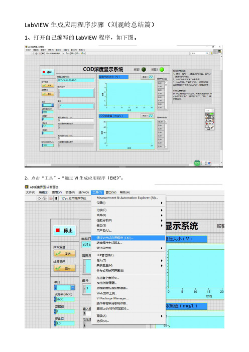
LabVIEW生成应用程序步骤(刘观岭总结篇)1、打开自己编写的LabVIEW程序,如下图。
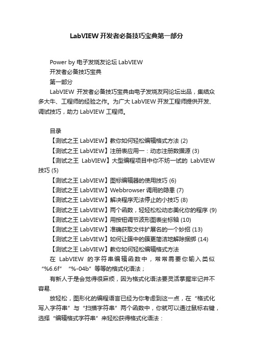
2、点击“工具”--“通过VI生成应用程序(EXE)”。
3、选择路径保存项目,点击“继续”。
4、可更改程序生成规范名称、目标文件名、目标目录。
点击“生成”。
5、生成后界面如下图所示,点击“完成”。
6、点击“完成”后,出现下图所示的项目界面。
点击保存按钮()。
7、此时生成的文件只能在安装了LabVIEW的电脑上运行,需要封装上一些插件。
右击“程序生成规范”--“新建”--“安装程序”。
8、生成界面如下图。
产品信息可以更改程序生成规范名称、产品名称、安装程序目录。
此处重点有两个地方“源文件”和“附加安装程序”。
(1)“源文件”:将刚才生成的应用程序(此处为AD采集界面)和vi程序(此处为AD采集界面.vi)均添加到右边。
(2)“附加安装程序”:将自动选择推荐的安装程序去掉,自主选择。
可去掉些用不到的。
若用串口通信,必须选择NI-VISA选项。
点击“生成”。
9、下图是安装完成界面,点击“完成”,再次点击“”。
10、按照步骤8的“安装程序目录”(图片已复制过来)找到“我的安装程序”文件夹。
11、将“我的安装程序”文件夹拷贝到任何电脑(无论有无安装LabVIEW)上均可运行。
文件中内容所下图所示,运行“setup.exe”即可安装本程序。
完成讲解。
LabVIEW的文件管理操作节点图标及其功能

LabVIEW 的文件管理操作节点图标及其功能
文件管理操作VI 和函数节点位于函数选板的“编程→文件I/O→高级文
件函数”子选板,如图1 所示。
其中包括文件管理操作和文件路径操作。
文件管理又包括对文件的操作和对文件目录的操作。
文件操作包括移动、复制、删除文件以及修改文件特性;文件目录的操作包括创建目录、列出目录内容。
表1 详细列出了文件管理操作节点的图标和功能。
文件管理操作节点中还包含一个Express VI——文件对话框,其图标和接线端如图2 所示。
文件对话框Express VI 的输入和输出接线端说明如下。
按钮标签:指定确定或当前目录按钮中的标签,如果标签超过按钮的长度,则超过的部分不显示。
表1 文件管理操作子选板。
LabVIEW中生成应用程序

LabVIEW中生成应用程序预览说明:预览图片所展示的格式为文档的源格式展示,下载源文件没有水印,内容可编辑和复制LabVIEW中生成应用程序将所有需要的文件,包括主vi 和所有子vi,以及用到的文本文件等附属文件,都放置到一个文件夹中,并确保所有程序都能正确执行。
我们在这里把它们都放在“示波器”文件夹里。
图中选中的是这个程序的主VI,打开LabVIEW2012,点击文件》新建,在打开的“新建对话框”中选择“项目”,并点击确定按钮完成新建。
之后LabVIEW自动打开项目浏览器,如下所示:在“我的电脑”上右键,选择添加》文件夹(自动更新)。
在弹出的“选择需插入的文件夹”对话框中打开我们要添加的文件夹:然后点击右下角的“当前文件夹”,即可添加当前文件夹到项目中,添加好之后的效果如下:点击文件》保存全部(本项目),在打开的“命名项目”对话框中文件名处输入项目名,这里我们输入“虚拟示波器。
点击确定保存项目。
在项目中右键程序生成规范,选择新建》应用程序(EXE):弹出“应用程序生成器信息”对话框。
点击确定即可。
接下来,将会弹出“我的应用程序属性”对话框:在“程序生成规范名称”中输入“虚拟示波器项目”,“目标文件名”里输入“虚拟示波器”,输好之后的效果如下:在左边的“类别”里选择“源文件”,在中间的项目文件里,展开示波器,选中虚拟示波器.vi并将其添加到启动VI栏里:在“类别”栏选择“图标”,不勾选“使用默认LabVIEW图标文件”,这时自动弹出“选择项目文件”对话框:点击添加,选择一个ico格式的图标文件,添加后的效果如下:在“类别”栏里选择“预览”,点击右边的“生成预览”,生成成功的效果如下:预览成功,就可以点击下边的“生成”按钮了。
然后弹出一个“生成状态”窗口,表明生成的进度。
生成完成后点击“完成”按钮。
再次保存本项目,然后关闭项目浏览器。
LabVIEW开发者必备技巧宝典第一部分
LabVIEW开发者必备技巧宝典第一部分Power by 电子发烧友论坛LabVIEW开发者必备技巧宝典第一部分LabVIEW 开发者必备技巧宝典由电子发烧友网论坛出品,集结众多大牛、工程师的经验之作。
为广大LabVIEW 开发工程师提供开发、调试技巧,助力LabVIEW 工程师。
目录【测试之王LabVIEW】教你如何轻松编辑格式方法 (2)【测试之王LabVIEW】注册表应用一:动态注册数据源 (3)【测试之王LabVIEW】大型编程项目中你不妨一试的LabVIEW 技巧 (5)【测试之王LabVIEW】图标编辑器的使用技巧 (6)【测试之王LabVIEW】Webbrowser调用的隐患 (7)【测试之王LabVIEW】解决程序无法停止的小技巧 (8)【测试之王LabVIEW】两个函数,轻轻松松动态美化你的程序 (9) 【测试之王LabVIEW】用按钮调节波形图表坐标轴 (10)【测试之王LabVIEW】准确获取文件扩展名的一个妙招 (13)【测试之王LabVIEW】如何让簇中的簇更简洁地解除捆绑 (14)【测试之王LabVIEW】教你如何轻松编辑格式方法在LabVIEW的字符串编辑函数中,常常需要你输入类似“%6.6f”“%-04b”等等的格式化语法;有新人于是会觉得很麻烦,因为格式化语法要灵活掌握牢记并不容易.放轻松,图形化的编程语言已经为你考虑到这一点,在“格式化写入字符串”与“扫描字符串”两个函数中,你就可以通过鼠标右键,选择“编辑格式字符串”来轻松获得格式化语法:你只需要在弹出的编辑框中选择你需要的格式化操作,LabVIEW 就会自动在“格式字符串”输入端生成相应的格式化语法输入~ 是不是很简单呢?动手试一试吧!【测试之王LabVIEW】注册表应用一:动态注册数据源LabSQL与数据库之间是通过ODBC连接,用户需要在ODBC中指定数据源名称和驱动程序。
因此在使用LabSQL之前,首先需要在Windows操作系统中的ODBC数据源中创建一个DSN(Data Source Name,数据源名)。
LabVIEW文件操作介绍

1.打开/创建/替换文件函数
图6-1
文件I/O子模板
2.关闭文件函数
图6-3 图6-2
关闭文件函数接线端子
打开/创建/替换文件函数接线端子
3.格式化写入文件函数
图6-4
格式化文件函数接线端子
4.扫描文件函数
图6-5
扫描文件函数接线端子
6.3 常用文件类型
6.3.1 文本文件
文本文件是最常用的文件类型。 LabVIEW提供两种方式创建文本文件。 一种方式就是使用打开/创建/替换文件函数。
第六章 文件操作
6.1文件类型 6.2文件I/O函数
6.1 选择合适的文件类型
LabVIEW支持的文件类型
文本文件(Text Files) 表单文件(Spreadsheet Files) 二进制文件(Binary Files) 数据记录文件(Datalog Files) XML文件 配置文件(Configuration Files) 波形(Waveform)文件 基于文本的测量文件(.lvm文件) 数据存储文件(.tdm文件) 高速数据流文件文件(.tdms文件)
小试身手
1. 文本文件和二进制文件的主要区别是什么?
2. 请说出下面这几种文件是文本文件还是二进 制文件:数据记录文件(Datalog Files), XML文件,配置文件,波形文件,LVM文件, TDMS文件。
小试身手
3. 有一个测量程序,采集 两路信号,每1s采集一次, 要求每采集一次,就将采 集结果写入文本文件尾部, 即使重新运行程序,仍能 保证数据添加到文件尾部, 而不会覆盖原有数据。格 式为a保留4位小数,b为整 数,如右图所示。
我和LabVIEW
当我开始在键盘上敲打出这句话的时候,我已经使用 LabVIEW 7 年了。
7 年的时间,就算天赋平平也可以积攒下一箩筐可供参考的经验了。
所以我打算利用今后的闲暇时间写一些这方面的东西,既可以同大家交流,也是作为自己这七年工作的总结。
还是在上大学的时候,有一次老师让编写一段软件,用来模拟一个控制系统:给它一个激励信号,然后显示出它的输出信号。
那时我就想过,可以把每一个简单的传递函数都做成一个个小方块,使用的时候可以选择需要的函数模块,用线把它们连起来,这样就可以方便地搭建出各种复杂系统。
后来,我第一次看到别人给我演示的LabVIEW编程,就是把一些小方块用线连起来,完成了一段程序。
我当时就感觉到,这和我曾经有过的想法多么相似啊。
一种亲切感油然而生,从此我对LabVIEW的喜爱就一直胜过其他的编程语言。
LabVIEW 的第一个版本发布于1986年,是在 Macintosh 机上实现的,后来才移植到了PC机上,并且LabVIEW 从未放弃过对跨平台的支持。
这也给 LabVIEW 带来了一些麻烦。
最明显的就是LabVIEW开发环境的界面风格。
它总是与一般的 Windows 应用程序有些格格不入:面板是深灰色的,按键钮是看起来别别扭扭的 3D 模样。
还有一些可能不太容易发现:比如对于整数的存储,LabVIEW即便是运行在x86系统上,采用的也是高地址位存高位数据(big-ending)。
这与我们习惯了的x86 CPU使用的格式正相反,这往往给编写存取二进制文件带来了不多不少的麻烦。
我接触过的最早的LabVIEW版本是4.0版,发布包是一个装有十几张三寸软盘的大盒子。
安装的时候要按顺序把软盘一个一个塞到计算机里。
尽管当时LabVIEW的界面不是很好看,但我还是非常喜欢它。
真方便呐!比如说要画一个开关,用 LabVIEW 一拖就行了。
如果要自己动手用 C 语言设计一个好看的开关,,那得费多少时间啊!我尤其喜欢它通过连线来编程的方式,尽管很多熟悉了文本编程语言的人刚开始时会对这种图形化编程方式非常不适应。
LabVIEW中二进制文件的存储与读取方法

LabVIEW中二进制文件的存储与读取方法背景在软件开发中,二进制文件格式相对于文本文件格式的缺点是,没有文本文件通用性强、直观,同时,在读取文件数据时,用户需要知道存储数据的数据类型格式等,才可以准确还原文件内容,但是,二进制文件的优点也比较突出,如文件存取速度快、占用空间小,同时,也可有效保护自己的数据文件。
在上篇文章中已经详细说了LabVIEW平台中文本文件的读写编程方法,这次通过例子再说下二进制文件的编程方法。
例1:入门例子例子要求:将1至16共16个32位的整型数字以二进制文件的格式存储到计算机的D盘上,文件名称为“test1.bin”,存储完成后,立即读出该文件内容,并显示到前面板的数组控件上。
程序运行后界面如下图所示:实现代码如下:用For循环产生32位的整型数字1-16,读写二进制文件同读写文本文件的步骤相同,依照着打开文件、读写文件、关闭文件的顺序执行。
对于“写入二进制文件”函数的主要参数说明如下:l 待写入的数据参数,其类型可以连接任意的数据类型,即可以将任意数据写入二进制文件;l 是否预置数组或字符串的大小参数,表明当数据为数组或字符串时,LabVIEW是否将数据大小信息添加至文件开头,当为真时,在写入数据时,先写入4个字节的数值,存储了待写入数据的大小,默认为真,此例该参数设为假,即文件的开头未保存数组长度信息。
l 字节顺序,可以是大端、小端或主机字节顺序,例子中使用的是大端序,其特点是最高有效字节占据最低的内存地址,默认是大端序。
本例字节顺序使用的是大端序,存储后文件内容以十六进制格式显示如下,对于1-16之间的32位整型数字明显看出,如对于数字1,低内存地上存储的是数据的高位字节(00),而高内存地址上存储的是数据的低位字节(01):当以小端序存储时,存储后文件内容以十六进制格式显示如下,其字节顺序与大端序相反:对于“读取二进制文件”函数的主要参数说明如下:l 读取文件的数据类型参数,必须给一个参数,该参数与写入文件时数组类型完全一致;l 读取数据的个数,不接该参数时,只读取一个数值,为-1时,读取所有的数据,本例为-1,表示读取整个文件的数据,为其它值时,读取相应个数的数据。
LabVIEW 2009 发行说明说明书

LabVIEW发行说明™LabVIEW 2009发行说明包含LabVIEW安装说明和LabVIEW的操作系统要求。
如升级LabVIEW前期版本,安装LabVIEW 2009前应阅读软件升级包中的LabVIEW升级说明。
如需转换前期版本的VI,在LabVIEW 2009中使用,必须阅读相关注意事项。
安装LabVIEW前,应阅读本文档的系统要求部分,然后按照安装LabVIEW 2009中的说明进行安装。
安装LabVIEW后,请阅读参考资料部分,了解LabVIEW入门知识。
目录系统要求 (2)安装LabVIEW 2009 (5)Windows (5)Mac OS (6)Linux (7)安装LabVIEW附加软件 (8)安装应用程序生成器 (8)激活LabVIEW许可证(Windows) (8)试用LabVIEW、模块和工具包 (9)单用户许可证和批量许可证 (9)安装和配置硬件 (9)Windows (9)Mac OS (9)Linux (10)参考资料 (10)LabVIEW快速参考指南 (10) (10)系统要求表1为运行LabVIEW 2009的操作系统要求。
表1LabVIEW 2009的系统要求系统平台磁盘空间和系统要求重要说明所有平台运行LabVIEW至少需要256 MB的内存。
NI建议使用1 GB或以上的内存。
运行LabVIEW至少需要1024 × 768像素的屏幕分辨率。
部署LabVIEW生成的应用程序时,LabVIEW运行引擎至少需要64 MB的内存,屏幕分辨率至少为800 × 600像素。
NI建议使用256 MB以上的内存且屏幕分辨率至少为1024 × 768像素。
LabVIEW和LabVIEW帮助包含16位彩色图形。
LabVIEW至少需要16位彩色设置。
如需查看或搜索PDF格式的LabVIEW用户手册,需安装Adobe Reader 6.0.1或更高版本。
- 1、下载文档前请自行甄别文档内容的完整性,平台不提供额外的编辑、内容补充、找答案等附加服务。
- 2、"仅部分预览"的文档,不可在线预览部分如存在完整性等问题,可反馈申请退款(可完整预览的文档不适用该条件!)。
- 3、如文档侵犯您的权益,请联系客服反馈,我们会尽快为您处理(人工客服工作时间:9:00-18:30)。
Storing data in a fileStarting with a set of data as if it were generated by a daq card reading two channels and 10 samples per channel, we end up with the following array:Note that the first radix is the channel increment, and the second radix is the sample number. We will use this data set for all the following examples.The first option is to send it directly to a spreadsheet file.The data is wired to the 2D array input and all the defaults are taken. This will ask for a file name when the program block is run, and create a file with data values, separated by tab characters, as follows:1.0002.0003.0004.0005.0006.0007.0008.0009.000 10.00010.000 20.000 30.000 40.000 50.000 60.000 70.000 80.000 90.000 100.000Note that each value is in the format x.yyy, with the y’s being zeros. The default format for the write to spreadsheet VI is “%.3f” which will generate a floating point number with 3 decimal places. If a number with higher decimal places is entered in the array, it would be truncated to three.Since the data file is created in row format, and what you really need if you are going to import it into excel, is column format. There are two ways to resolve this, the first is to set the transpose bit on the write function, and the second, is to add an array transpose, located in the array pallet.The new data output now will look like:1.000 10.0002.000 20.0003.000 30.0004.000 40.0005.000 50.0006.000 60.0007.000 70.0008.000 80.0009.000 90.00010.000 100.000Note that it is now in column format with what was the first row, now in the first column. This gives you the first acquired channel in the first column and the second channel in the second column. This is a handy way to deal with the data in a spreadsheet. One problem with this format is that there are no labels or indicators to determine what is what in the file. We can address that in a moment.Frequently you want the data to be saved in a file that already exists, adding to the data that is there. This function allows that by setting the “append” input to True.Running this snippet against the file we created above gives the following output.1.000 10.0002.000 20.0003.000 30.0004.000 40.0005.000 50.0006.000 60.0007.000 70.0008.000 80.0009.000 90.00010.000 100.0001.000 10.0002.000 20.0003.000 30.0004.000 40.0005.000 50.0006.000 60.0007.000 70.0008.000 80.0009.000 90.00010.000 100.000The real advantage to this method is that this VI is extremely efficient at doing the write function, making it a very fast way to save large amounts of data. As stated before, the largest drawback is that you have to know about the data, and remember it later. Because of this, a number of users prefer to deal with the files as raw text, which is what they really are.This code snippet adds a step before the spreadsheet save that provides a title to the tow columns as well as the units. This example shows this as a discrete string build with a string concatenation, but it could be just as easily done with a single string constant as shown below. It is important to remember that “\t” is a tab character and the “\n” is a new line character. Also you must be sure that you have turned on the “ ‘\’ codes display “ option for the string, which is found in the right cli ck menu.The data file generated by either of these methods are the same, and shown below.Chan1 Chan 2Volts Volts1.000 10.0002.000 20.0003.000 30.0004.000 40.0005.000 50.0006.000 60.0007.000 70.0008.000 80.0009.000 90.00010.000 100.000This process works well for a large number of data points, but can also be used for a very small number of points. The only requirement is that there must be a full array, that being a data point in each row and column with no blanks. If you are using a single row of data you can use the 1D input to the write.It is often advantageous to mix text and numbers in the same file, even more than just column headers. Dates, times and units labels mixed with the lines prevent the spreadsheet write method from being used. To accomplish this a different tactic must be used.Most all files that are used for data storage are text files of some sort or another. There is nothing that prevents individual lines from being written as text for later use by other programs. This type of storage is typically done for either long term data or small amounts of data, since the process is very inefficient.The first step in this method is to determine the size of the array. This is easily done using array size.The output of the array size object is an array of integers, representing the size(s) of the array. In a 1D array, there is a single element that is the length of the array, however in a multi dimensional array, there is an array of sizes, each element of the integer array being one of the array dimensions. In the case of our sample, element 0 of the array is the number of channels and element 1 is the number of samples for each channel. The index array object allows us to break out the second element, which we will need to process the array.In the following snippet I have dropped an index array object into a for loop and wired it to the 2D array. LabVIEW does something here that will bite you if you’re not careful. Notice how the wire changes from a double wide line to a single heavy line and there is a small square with brackets inside where the line crosses into the for loop. LabVIEW is trying to be helpful, and realizing that it is an array coming in, it will automatically index the array.Automatic indexing is a feature that can be very useful, and can also be a real pain. In the above snippet, the loop count (the little N box) is set to the first dimension of the array, in this case 2. For each iteration of the loop, the line inside the box (orange 1D array line) will have the 10 elements associated with the first row of the array. Nothing else of the array is visible inside the for loop. The second iteration will have the second row of the array, and if there were more rows, this would continue until the array was out of rows. Since we need to see both channels at the same time, we have somechoices. We can turn off the indexing, by right clicking on the box and selecting “Disable Indexing”. This will turn the square solid orange and the entire array is now visible inside the for loop. Once this is done, we can then go through the array line by line and pull out each individual element as shown below.Each pass of the array will pull out the two channels from the array with the index array objects. This is a simple and straightforward way to accomplish this task. It is easy to read at a later time and pretty obvious to anyone who is working with the program later just what is being done.A slightly more elegant method makes use of auto indexing.In this example, the for loop is iterated ten times, based on the number of rows in the transposed array. For each row, the index array objects pull out the channel 1 and channel 2 data, which could then be fed to some other function. In this case we are going to convert it to a string and write it to a file. The entire program section is shown below.While the technique is used here to write a single 2D array, it is easy to apply this technique to an application where the data is taken at long intervals and written to a text file so the data is not lost in the event of a computer hiccup or gurgling cringing death….The data output is shown following the program snippet.Chan 1 Chan 2Volts Volts1.000 10.0002.000 20.0003.000 30.0004.000 40.0005.000 50.0006.000 60.0007.000 70.0008.000 80.0009.000 90.00010.000 100.000The file storage portion consists of three blocks, one which is run only on the first iteration, and the other three that are run every iteration. The initial function, “open/Create/Replace file” is used without any path input to cause the prompt for a file. This will then create the file if it is not in existence, or open it if it is. This is located inside a case statement that executes only when the iteration counter is 0. In addition it appends the file header information to the string of data values. Once this has been done a value known as a reference number, which is how the computer refers to the file, is passed to a block which gets the file size. If the file is a new file, the size is 0. If not, it returns the total number of bytes in the file.The third block in the string is a “set File Position”. This block moves a pointer in the file to a particular position. In our case we have wired the output of the Get File Size to the input of the Set File Position so that the pointer is now pointing to the end of the file. The last block is a Write to Text File. This block begins writing the text string wired to its input at the location that the pointer is at, in our case, the end of the file. This set of blocks effectively appends the string to the existing file, even if that length is zero. The reference number is sent to a shift register so it is available for the next iteration of the loop.In the next and all subsequent iterations of the for loop, the iteration counter is not equal to 0, so the FALSE case is executed, which does nothing but pass the string and reference number values back on out to the program.。