A note on the Gauss map of complete nonorientable minimal surfaces

合集下载

Notes On Hilbert's 12th Problem

a rX iv:mat h /6511v1[mat h.NT]3M a y261NOTES ON HILBERT’S 12TH PROBLEM SIXIN ZENG Abstract.In this note we will study the Hilbert’s 12th problem for a primitive CM ﬁeld,and the corresponding Stark’s ing the idea of “Mirror Symmetry”,we will show how to generate all the class ﬁelds of a given primitive CM ﬁeld,thus complete the work of Shimura-Taniyama-Weil.Introduction 0.1.Let K be a number ﬁeld,H K be the ideal class group of K ,and let K 0be the Hilbert class ﬁeld of K .The class ﬁeld theory tells us there is a canonical isomorphism Gal (K 0/K )≃H K .In general given any integral ideal d ,let K d be the maximal abelian extension of K unramiﬁed outside d ,and let H d be the generalized ideal class group relative to d ,then a similar isomorphism holds as well:Gal (K d /K )≃H d .On the other hand,Hilbert’s 12th problem asking for an explicit generation of all the abelian extension of K ,more precisely it is asking for ﬁnding a special transcendental function,whose values at some special points would generate all the abelian extension of K .When K is the rational ﬁeld Q ,the transcendental function is the exponen-tial function and the special points are the division points on the unit circle.Indeed by the classical Kronecker-Weber theorem,all the abelian extension of Q can be obtained by adding the roots of unity to Q .When K is an imaginery quadratic ﬁeld,this problem is answered by the theory of complex multiplications.As this theory has very much inﬂuenced the later thinking about this problem,let’s recall some details.So let K be such a ﬁeld,consider the set of elliptic curves E satisfying End (E )⊗Q ≃K ,i.e.,the set of elliptic curves with complex multiplications by K .All such elliptic curves can be constructed by the following way:take the caononical embeddingι:K −→C ,let a be an integral ideal of K ,then a is a rank 2Z -module in C ,i.e.,ι(a )is a lattice in C ,so we can take the quotient C /ι(a )which is an2SIXIN ZENGelliptic curve with complex multiplication by K.From the construction it is clear that the ideal group of K operates on this set of elliptic curves,indeed for any representative b of an ideal class,we have the isogeny:C/ι(a)→C/ι(ab). On the other hand all such elliptic curves are deﬁned over some numberﬁeld, and they are represented by the moduli points on the moduli space of all elliptic curves M1=H/P SL2(Z).In particular the Galois group acts naturally on the moduli points of this set of elliptic curves.So if E=C/ι(a),let℘be a prime of K,E(℘)=C/ι(a℘),s(℘)∈H K≃Gal(K0/K)the Artin symbol,then the main result of the complex multiplication is E s(℘)≃E(℘).In more concrete terms if j is the classical modular function,and let p E be the moduli point of E on M1=H/P SL2(Z),then j(p E)is an algebraic number and generates the Hilbert classﬁeld of K.Similar statements hold for all the ray classﬁelds of K.The idea behind the theory of complex multiplication can be summerized as the following:•Given the numberﬁeld K,in order to solve the Hilbert’s12th problem,ﬁrst we need toﬁnd a suitable class of algebro-geometric objects X,say varieties;•X should be closely related to K such that the ideal classes of K cannaturally act on them;•All such X should be deﬁned over some numberﬁeld,all such X shouldbe living on some natural moduli space so theirﬁeld of moduli are givenby the coordinate function evaluated at the moduli points.The Galoisgroup can naturally acts on them;•Moreover the action of the ideal classes of K and the action of Galoisgroup on the moduli points should be related by the reciprocity law ofclassﬁeld theory and the Kronecker congruence relations;If we canﬁnd such a class of X,then theﬁeld of moduli of X give the answer to Hilbert’s12th problem.For a general numberﬁeld besides imaginery quadratic,this philosophy is diﬃcult to apply.So from now on we will concentrate on a special case.From now on let K be a primitive CMﬁeld of degree2n,n≥1.K is then an imaginery quadratic extension of a totally realﬁeld F,with[F:Q]=n. Further let K∗be the reﬂexiveﬁeld of K,F∗be the maximal totally real subﬁeld of K∗,then K∗is also a primitive CMﬁeld of degree2n,[K∗:F∗]=2. Let{σ1,σ2,···,σn}be the set of archemidean primes of F,lifted to K as the CM types,and letρbe the complex conjugate.When n>1,according to the above philosophy,we naturally consider the set of abelian varieties of dimension n with complex multiplication by K with CM type{σ1,σ2,···,σn},i.e.,those abelian varieties satisfying End(X)⊗Q≃NOTES ON HILBERT’S12TH PROBLEM3 K,and moreover for anyα∈K the action ofαon the space of holomorphic diﬀerentials of X is given as the diagonal action of diag(ασ1,···,ασn).All such X can be constructed in the following way:letι:K→C n be the embedding ι(x)=(xσ1,···,xσn),then for any integral ideal a,ι(a)⊂C n as a Z-lattice is of rank2n,hence the quotient X=C n/ι(a)is an abelian variety,one see that such X satisfying the above conditions.From the construction such set of abelian varieties are naturally associated to K,with the integral ideals of K act on them as isogenies.This is exactly the same as elliptic curves.So next we shall consider the moduli space for these X and their arithmetic properties,it is here some complication arised,let’s be careful.Let O K and O F be the rings of integers of K and F,and let a be an integral ideal of O K.Regarding a as a module of O F,it is of rank2.More precisely we have the following(see for example,Yoshita’s book[19]):Lemma0.1.For any ideal a of O K we have the isomorphism as O F-module: a≃b·ω1⊕O F·ω2,whereω1,ω2∈K,b a fractional ideal of O F.Moreover the ideal class of b is c·N K/F(a)=c·aaρ,where c is a fractional ideal of F, independent of a,and c2=D K/F.In particular O K=c·ω1⊕O F·ω2,and if a satisfying a·aρ=(µ),then a=c·ω1⊕O F·ω2.Now let X=C n/ι(a),by Shimura the polarization of X is given by the Riemann form E(x,y)which is E(x,y)=T r K/Q(ζxyρ),withζ∈K satisfying ζρ=−ζ,Im(ζσi)>0,any i.The“type”of this polarization,by deﬁnition,is the ideal class ofζd K/F aaρ,where d K/F is the relative diﬀerent of K over F. From the above lemma it is clear that b is the type of X.For any moduli problem,in order to have a good moduli space we need to ﬁx a polarization of X.For our class of X,we observe that they all have a large ample cone,in fact the dimension of the ample cone are all of n,hence it makes sense to consider the moduli problem with all the ample classesﬁxed. This is the moduli space of“type polarized abelian varieties”.Concretely for any fractional ideal b of O F,we can constructed a moduli space M n(b)which parametrizes families of abelian varieties with the form C n/v n·ι(b)⊕ι(O F),where v n is a vector in the product of upper half plane H n,and the dot product is deﬁned component-wise.It is well-known that M n(b)=H n/Γ(b)withΓ(b)={α∈SL2(O F)|α≡1mod(b)}.If X is the above abelian variety of type b,the X=C n/ι(a)with a=b·ω1⊕O F·ω2, up to isomorphism we can chooseω1,ω2∈K such thatωX=ω1/ω2satisfyingIm(ωσiX )>0for any i,i.e.(ωσ1X,···,ωσnX)is a vector in H n,hence deﬁnes amoduli point of X in M n(b).4SIXIN ZENGSo in summary given the class of CM abelian varieties with aﬁxed CM type,we can construct a natural moduli space M n(b)for aﬁxed type of X,i.e.,ifX1,X2are of the same type,they live on the same moduli space,but diﬀerenttypes can produce diﬀerent moduli spaces.So although the ideal classes of Kcan act on all of the X,the Galois group can only act on the subclass of Xwith the same type.On the other hand it is easy to show that all X are deﬁned over aﬁniteextension of the reﬂexﬁeld K∗.In fact for an ideal a∗of K∗,we deﬁnea=g(a∗)= τi a∗τi,where{τ1,···,τn}is a CM type of K∗,then g(a∗) acting on X will not change the type of X.It is from this point of view thatin1955,Shimura-Taniyama-Weil(see Shimura’s book[12])established that theﬁeld of moduli of X will generate part of the classﬁeld of K∗,precisely it isthe classﬁeld corresponding to the subgroup of the ideal class group H0K∗= {a∈H K∗|g(a)=(µ),µ∈K}.0.2.In this note we will try to extend the work of Shimura-Taniyama-Weil to cover all the classﬁelds of K.There are actually two problems here.First, the appearance of the reﬂexﬁeld K∗is quite inconvenient,since our abelian varieties X,their moduli spaces M n(a),and the CM points on the moduli are all constructed naturally from the given CMﬁeld K,it is natural for us to look for the invariants from these abelian varieties that directly generate the class ﬁelds of K,instead of the reﬂex K∗.Second and more important problem,is how can we deal with the classﬁelds that corresponding to the isogenies of abelian varieties that live on the diﬀerent type of moduli spaces.Theﬁrst problem can be solved in the following way.Since theﬁelds K and K∗are reﬂex to each other,by Shimura-Taniyama-Weil theory,the classﬁelds of K is generated by the abelian varieties associated to K∗.So the problem is toﬁnd invariants on X that somehow related to Shimura varieties associated to K∗.For this purpose Iﬁnd the following notion of“cone polarized Hodge Structure”quite useful.First we observed the for all the abelian varieties of the CM type the Kahler cone is very large.Indeed as the polarizations are determined by the Riemann form E(x,y)=T r K/Q(ζxyρ),so the polarizations are determined byζ∈K such thatζρ=−ζ,Im(ζσi)>0,any i.Suchζform a cone of dimension n, hence the Kahler cone is of n dimensional.We can also see this by the fact that since End(X)is an order in K,the automorphism group of X is then the unit group of the order,which is of the form Z n−1⊕T orsion.So the Kahler cone of X is necessarily n dimensional.Given such Kahler cone C X of X we can consider the primitive classes of X in the middle dimension relateive to this cone,i.e.,those classes of dimension n such that are annilated by any element in the Kahler cone.NOTES ON HILBERT’S12TH PROBLEM5{α∈H n(X,C) α·x=0,∀x∈C X}This is the generalization of the notion“transcendental lattice”in the theory of K3surface.The Kahler cone and these primitive classes relative to this cone should be considered as the most basic Hodge theoretical invariants of our abelian varieties.So to understand these abelian varieties,we need to construct the appropriate moduli spaces for these invariants.First let’sﬁx the Kahler cone and consider the primitive classes of the middle degree relative to this cone.Such primitive classes carries a natural Hodge structure,indeed for abelian varieties with F-multiplication the primi-tive classes can be characterized as the invariant classes of the automorphism group U F,it carries a Hodge structure of weight n,with the i-th Hodge number to be i n =n!6SIXIN ZENGTheorem0.2.(1)We have a natural isomorphism M P H≃H n/SL2(O F∗);(2)The natural morphisms M n(a)→M C→M P H are allﬁnite.By the theory of Shimura-Taniyama-Weil,the moduli points of X on this moduli space will generate the classﬁeld of K.The natural modular function on the Hilbert modular variety of K∗,when pulled back to M n(a),will become a natural modular function on M n(a).In this way,by directly considering the geometry of X,we can have the classﬁelds of K generated.This answers our ﬁrst question.Note that in our approach we do not emphasis on the use of“ﬁeld of moduli”, indeed since our moduli space of primitive Hodge structures can actually be regarded as the moduli space of abelian varieties with multiplication by F∗,the natural“ﬁeld of moduli”somehow lose its meaning on this moduli space(1). We only need the natural modular functions on the moduli spaces,which give the coordinates of the CM points.In any case our approach is more natural in view of Hodge theory,and serve the purpose of generating classﬁelds of K well.0.3.The second question is more diﬃcult.We need toﬁnd a natural way to interpolate the moduli spaces of diﬀerent types.For this purpose we will use the idea of Mirror Symmetry.Precisely if R1and R2are two ideals suchthat R1R−12is a real ideal,then although the abelian varieties X R1and X R2deﬁned by R1and R2are living on the diﬀerent moduli space,we will showtheir“Mirror partners”X′R1and X′R2are living on a single moduli,and theMirrors’ﬁeld of moduli can be used to generate the classﬁelds.To motivate our idea,let’s consider another approach to the Hilbert’s12th problem,namely the Stark’s conjectures([16]).The point of departure is to consider the Dedekind zeta function and Hecke L-functions for the numberﬁelds.Hilbert’s problem asks for a natural tran-scendental function,indeed for the abelian extension point of view,nothing can be more natural than these L-functions,as they transformed under the Galois group ually the Stark’s conjectures are formulated and studied for a totally realﬁeld,but as we shall see,it is more natural and sim-ple to study it for the CMﬁeld,because all theﬁnite extension of CMﬁelds are necessarily CM,i.e.,any extension of K has no real inﬁnity.The remarkable fact about the Stark’s conjectures is that it can be for-mulated on any classﬁelds of K uniformly,not just those classﬁelds in the Shimura-Taniyama-Weil theory,so in the explicit form it can be used as a guide for us to search for the solution of missing classﬁelds of the old theory.NOTES ON HILBERT’S12TH PROBLEM7 So let K as above,let R be an ideal class of K,recall that the Dedekind zeta function is deﬁned asζK(s)= a1s−1κK+ρK+O(s−1)whereκK=(2π)n R KN(a)s .NatuallyζK(s)= RζK(s,R),with the limitformula:ζK(s,R)=κw Ks n−1(1+δK(R)s)+O(s n+1) thenδK(R)=nγ+nlog2π−log|D K|−w K|D K|1/2ρK(R−1)w Ks n−1(1+δK s)+O(s n+1) withδK= RδK(R)•ifχ=χ0is not trivial,thenL K(s,χ)=ζK(s,R)=−R Kw K0=(−1)m(R K8SIXIN ZENGThe Stark’s conjecture predicts that if we write L K(s,χ)=R K(χ)s n+ O(s n+1),then R K(χ)also has the form of regulators,i.e.it is a determinent of a matrix whose entries are linear combination of logarithm of units of K0. Moreover we should expect R K(χ)σ=R K(χσ)for anyσ∈Aut(C).In our present case K is a primitive CMﬁeld,in this case Stark’s conjec-ture is somehow simple in the following sense:the regulator R K of K is a determinent of(n−1)×(n−1)matrix,and the regulator R Kof K0is a determinent of(mn−1)×(mn−1)matrix.Stark’s conjecture in fact says that the quotient R K/R K is a determinent of(mn−n)×(mn−n)matrix, and this matrix should be diagonalized into m−1blocks,with each block a n×n matrix,further in this case we can use the R K matrix to simplify these blocks,so in this extension there are only m−1essential new units.In other words,U Kas a module of U K is free of rank m−1.This is very much similar to the classical case of imaginery quadraticﬁelds.By some elementry argument we can show that R K=(R K)m·vol(S), where vol(S)is a determinent of(m−1)×(m−1)matrix whose entries are linear combinations of logarithm of units in K0.These are the basis of U Kas the module of U K.On the other hand by the Frobenius determinent formula, χ=χ( Rχ(R)δK(R))=det R1,R2=1(δK(R1)−δK(R2)) Hence we should expect:•δK(R)=log|ηK(R)|;•δK(R1)−δK(R2)=log|ηK(R1)ηK(R2)is a unit in K0.More overthese units should transform under the Galois group according to thereciprocity law.0.4.To prove things like this we need to have a good expression forδK(R), this can be done by using the theory of GL(2)Eisenstein series over the totally realﬁeld F.The Eisenstein series is deﬁned asE(w,s;a)=(c,d)∈(a⊕O F)/U F,(c,d)=(0)ni=1y s i|cσi z i+dσi|−2sThe idea is a classical one,sinceζK(s,R)= a∈R1w2satisfyingIm wσi>0,∀i.Then we haveNOTES ON HILBERT’S 12TH PROBLEM 9ζK (s,R )=N (a 1)s α∈a 1/U F ,α=012n −2πn h F RF [χF (d F )L F (2,χ−1F )i Im(ωi )+πn D −3/2F 0=b ∈d −1F a σ1,χ(bda )|N (b )|−1exp (2πi (n j =1b j ℜ(w j )+i |b j Im(w j )|))]where (1)a,d ∈A ×F such that div (a −1)=a and div (d )=d F ;(2)σs,χ(x )is a function deﬁned asσs,χ(s )= v ∈(finite primes ) 1+χv (w v )q s v +···+(χv (w v )q s v )ord v (x v )if x v ∈d v ,0if x v /∈d v .Here d v denotes the ring of integers of F v ,w v is the prime elementof F v and q v =|d v /w v d v |.So we haveζK (s,R )=−R K10SIXIN ZENGδK(R)=h(ω;a)−log i Im(w i)−logN(a)We reminded that a is the type of R−1,w=(w1,···,w n)∈H n is the CM point deﬁned by R,and h(w,a)is the complicated function deﬁned above.So our basic task is to understand this function.0.5.We notice that hχFsatisfying the following modular properties([19]):for γ∈Γa we have(1)hχF (γω;a)=hχF(ω,a)ifχF is not trivial;(2)h1(γω;a)−log( i Im(γω)i)=h1(ω,a)−log( i Imωi)So in particular we haveχFχF(a)hχF(γω;a)−log( i Im(γω)i)= χFχF(a)hχF(ω,a)−log( i Imωi)which suggests that we may actually have a Hilbert modular formηK(w;a) of parallel weight such that h(w;a)=log|ηK(w;a)|.Classically in case F= Q this is indeed the case asηK is the classical Dedekind eta functionη,it is well-known thatηhas an inﬁnite product expression,which when taking the logarithm translated into a Fourier expansion,which is exactly the above Fourier series.In the higher dimensional case it is not that easy2.Besides the fact that the Fourier expansion is too complicated and diﬃcult to work with,we can not expect by directly exponenciate the above expression of h to get a meaningful function,precisely because of the inﬁnite unit group of F,as shown as the regulator term R F in the leading coeﬃcients of the Fourier expansion.The regulator R F is not a rational number,in fact we expect it to be transcendental, so even if we exponenciate h we can not get anything useful for the arithmetic purpose.In particular we can not expect to get an inﬁnite product expression as the classicalηfunction.0.6.What should I do?It turns out although we can not exponenciate theh function,can not get the explicit formula forηK(w;a),we still can say something quantitatively about it.The idea is to consider a twisted version of Eisentein series:E u,v(w,s;a)=(c,d)∈(a⊕O F)/U F,(c,d)=(0)ni=1e2πi(cσi u i+dσi v i)(Im w i)s|cσi w i+dσi|−2sNOTES ON HILBERT’S12TH PROBLEM11 where(u,v)∈R n⊕R n.This is entirely adopted from the classical Kronecker’s second limit for-mula(see[18]).To explain why we need to develop the twisted Eisenstein series,let’s recall the classical situation,i.e.,when F=Q.In this case the Eisenstein series isE(w,s)=m,n∈Z,(m,n)=0(Im(w))s2[1+(CONST+log Im(w)−4log|η(w)|)s]+O(s2)The twisted Eisenstein series is:E u,v(w,s)=m,n∈Z,(m,n)=0e2πi(mu+nv)(Im(w))s24w∞n=1(1−q n w)and g u,v is the Siegel’s function:g u,v=−q1q zφ(w,z) and we haveg u,v=q112SIXIN ZENG(3)g u,v is also closely related to Dedekindη.In fact as a function of zg u,v has a simple zero at z=0withη(w)as the coeﬃcient,i.e.,|g u,v|=|η(w)|2|q z−1|+O(z2)This shows that the absolute value|η(w)|is not a theta null,but rather a“derivative theta null”.But we note our theta functions arenormalized at z=0to be zero,φ(w,0)=0,if the theta functionnormalized in this way,their derivatives can also be used as the coor-dinates on the moduli space.By abuse of notation we still call|η(w)|a theta null,hence it gives a modular function on the moduli space.From the deﬁnition,E u+1,v=E u,v+1=E u,v,hence g u+1,v=g u,v+1= g u,v,but since|g−v,u|=|q12B2(−v)w g−v,u(w)Then from the periodic condition of g u,v we immediately see that|φ(w,z+1)=φ(w,z);|φ(w,z+w)|=|q−1z|·|φ(w,z)| That is,|φ(w,z)|satisfying the characterization of a theta function,moreover since we know it is an analytic function,it then has to be a theta function itself.This is the idea we would follow in the higher dimensional case,as we observed before,since in the higher dimension we can not expect any explicit inﬁnite product formula for the functionηK(w;a),but we still have all the periodic properties as the1-dimensional case.Now we go back to the higher dimensional case,the Eisenstein series is:E(w,s;a)=(c,d)∈(a⊕O F))/U F,(c,d)=(0)ni=1(Im(w i))s|cσi w i+dσi|−2sWe have the limit formula:E(w,s;a)=−2n−2h F R F s n−1[1+(CONST+logN(a)+log( i Im(w i))−h(w;a))s]+O(s n+1) The twisted Eisenstein series is:NOTES ON HILBERT’S12TH PROBLEM13E u,v(w,s;a)=(c,d)∈(a⊕O F)/U F,(c,d)=(0)ni=1e2πi(cσi u i+dσi v i)(Im w i)s|cσi w i+dσi|−2sand we have the limit formula:E u,v(w,s;a)=−2n−2hF R F log|g−v,u(w;a)|s n+O(s n+1)where log|g−v,u(w;a)|has an explicit Fourier expansion,just like h(w;a).Then we argue as the following:(1)Recall that u=(u1,···,u n)∈R n,v=(v1,···,v n)∈R n,and O F⊂R n as a lattice.From the deﬁnition,for anyα∈O F,we have E u+α,v=E u,v+α=E u,v,i.e.,translate invariant under O F,hence|g−v+α,u|=|g−v,u+α|=|g−v,u|.(2)Now write z=u−vw,i.e.,z=(z1,···,z n),z i=u i−v i w i,∀i.We try to write g−v,u as a function of(w,z),so we deﬁneφ(w,z)=q−12B2(−v)w= i q−112wφ(w,z)|−log(|ηK(w;a)|2 i|z i|)}=0that islim z→0|q1|ηK(w;a)|2 i|z i|=1Also we verify that our theta function is normalized at z=0to be 0.This implies thatηK(w;a)is a theta null.By the classical theory of theta function,theta null naturally gives rise to the modular forms on the moduli space.In fact this should be more or less expected.By Mumford’s theory of algebraic theta function,we may further conclude that these theta nulls in fact deﬁnes the moduli space as an integral scheme over Z,hence have all the expected integral properties.14SIXIN ZENG0.7.In summary we have found the explicit form of the functionδK(R).δK(R)=logN(a)+log i Im(w i)−h(w;a)=logN(a)+log i Im(w i)−log|ηK(w;a)|2=log[N(a) i Im(w i)|ηK(w;a)−2|]where R is an ideal class of O K,a its type,w its CM point on M n(a),and ηk(w;a)is the theta null:∂∂z nφ(w,z)|z=0=ηK(w;a)2By the Stark’s conjecture,we need to understandδK(R1)−δK(R2),i.e., we need to understand the quotientηK(w1;a1)ηK(w2;a)is meaningful,as the modular function evaluating at the CMpoints,and the natural action of Galois group on them is prescribed by the reciprocity law.But when R1and R2are of the diﬀerent type,for example, when R1R−12is a real ideal,thenηK(w;a1)andηK(w;a2)are on the diﬀerent moduli spaces,thus their quotient becomes meaningless.This is precisely the limit of Shimura-Taniyama-Weil’s theory.So what can we do?To go further we need toﬁnd a natural way to inter-polate the diﬀerent moduli spaces,and it is here the idea of Mirror symmetry comes.As we shall see,in this case this quotient will have a meaning similar to the classical one if we consider the complexiﬁed Kahler moduli of the abelian varieties.Why should we interpolate the diﬀerent moduli spaces?The functionδK(R) is deﬁned not on a single moduli space of theﬁxed type,but rather automati-cally been deﬁned on all the moduli spaces,as the type a can vary accordingly. Likewise the modular formηK is a Hilbert modular form on all the type-ﬁxed Hilbert modular varieties,and when the type vary,can be regarded as a mod-ular form on all the moduli spaces.This strongly suggests that we should have a natural way to interpolate all these moduli spaces of diﬀerent types,such that these functions can naturally deﬁned.In other words,when weﬁx the type a,we get the Hilbert modular forms,what then happens if weﬁx the CM pointsωand let the type vary?When we look the explicit form ofδK(R)and h,we note the apparent symmetric roles played by the quantities σIm(ωσi)and N(a).Indeed if we ﬁx the CM pointsωand let a vary,we should have a meaning for the quantity N(a).This can be achieved by considering the Kahler moduli of our abelian varieties.0.8.Mirror Symmetry is usually formulated for the Calabi-Yau varieties, roughly it asserts that Calabi-Yau always come in pairs,X and X′,with theNOTES ON HILBERT’S12TH PROBLEM15“complex moduli”and“Kahler moduli”exchanged.In terms of the Hodgenumber,it means the Hodge diamond of X′is a rotation of X.For abelian varieties,Mirror Symmetry is generally regarded as“trivial”,as the underlying topological type would not change.Nevertheless we canstill talk about it.There are several constructions of Mirror manifold for theabelian varieties,the simplest one I believe,is given by Manin([9]).It goes asthe following:let k be any completeﬁeld,X an abelian variety over k,T bethe algebraic torus of dimension n over k,T≃(k×)n.Then the multiplicativeuniformization is0→P X→T→X→0,where P X is a free abelian groupof rank n,P X is called the period of X.Under this uniformization the Mirrorpartner X′is then0→P X→T∨→X′→0,i.e.,we explicitly indentify theperiods in T and T∨.When k≃C one verify that the complex moduli andKahler moduli of the two are exchanged.In our situation,given the Mirror pair X and X′we will be mainly concernabout the relations of theta functions on them.Since the underlying topologicaltype would not change,we may regard the Mirror transform as a“rotation”of complex structure of X.So to compare the theta functions on X and X′we have toﬁx the underlying real structures.We begin with X=C n/(w·a⊕O F)≃R2n/Z2n,any polarization of X isgiven by an integral skew-symmetric bilinear form on R2n.Given such a formω,we canﬁnd an integral basis{λ1,···,λ2n}of the integral lattice such thatif{x1,···,x2n}is the dual basis,thenω= n i=1δi dx i∧dx n+i,withδ1|δ2|···the elementary divisors.Note in our case the biliear form is given by the trace T r K/Q(ζxyρ)withthe admissibleζ∈K such thatζρ=−ζ,Im(ζσi)>0.Thus we may regard(x1,···,x n)as an integral basis of O F,and(x n+1,···,x2n)as an integralbasis of a.In particular(x n+1,···,x2n)depends on a.In the following we willdenote it as x n+i(a)if we need to use this dependence.Next we introduce the complex structure,so X becomes a complex tori,and we can introduce the complex coordinates.To do this let e i=λi/δi,i=1,2,···,n,and let{z i}be the complex dual of{e i}.Consider the changeof coordinates transform:Ω·(x1,···,x2n)T=(z1,···,z n)TThenΩ=(∆δ,Z)with∆δ=diag(δ1,···,δn)the diagonal matrix,and Zsymmetrical,Im(Z)>0.We recogonize that∆−1δZ is the period matrix of X.Note in our case for abelian varieties with CM by K,the peiod martix Z isnecessarily diagonal∆−1δZ=diag(w1,···,w n),with w=(w1,···,w n)∈H n.In particular we have z i=δi·x i+δi·w i·x n+i(a),we may regard it as the transform from the underlying real coordinates to the complex coordinates.16SIXIN ZENGNow recall the theta function on X is characterized by the periodic condi-tion:θ(z+λi)=θ(z);θ(z+λn+i)=e−2πiz iθ(z)Taking absolute values we have:|θ(z+λi)|=|θ(z)|;|θ(z+λn+i)|=e2πIm(z i)|θ(z)|However from the above coordinates transformation,Im(z i)=δi·Im(w i)·x n+i(a)The Mirror symmetry transform says that we can exchange the complex moduli with the Kahler moduli,while the coordinates w=(w1,···,w n)∈H n can be regarded as the complex moduli of X,where is the Kahler moduli?Our Kahler moduli coordinates are actually in the variables(x n+1(a),···,x2n(a)). Since they are depend on the type a,we want to write the dependency explic-itly,in order to understand the transformation of types.For this end let’s write x n+i=x n+i(O F).The type ideal a as a Z module,is a submodule of O F of full rank,i.e.,if weﬁx an integral basis of O F,then O F/a≃⊕n i=1Z/t i Z,with x n+i(a)=t i x n+i and i t i=N(a)/D F.Thus the positive rational numbers(t1,···,t n)can be conviniently regarded as the coordinates of the ideal a,and under appropriate identiﬁcation,can be regardedas the coordinates of of the Kahler class in the the Kahler moduli.So in particular we haveIm(z i)=δi·Im(w i)·t i·x n+iBut from the above formula,when we exchange the complex moduli(w1,···,w n) and Kahler moduli(t1,···,t n),it’s not going to change the multiplier e2πIm(z i)=e2πδi·t i·Im(w i)·x n+i.Since the absolute value of theta functions can be regardedas a real analytic function on R2n,thus we conclude that for the given Mir-ror pair X and X′,their theta functions’absolute values satisfying the same periodic condition,hence must be only diﬀered by a constant!Recall our previous puzzle,when two ideal classes R1and R2of O K sat-isfying R1R−12is a real ideal,then R1and R2are of the diﬀerent type,sothe corresponding abelian varieties X1and X2living on the diﬀerent moduli spaces,soηK(w,a1)/ηK(w,a2)has no meaning.But we knowηK(w,a)is the theta null of X,thus by the above formula,ηK(w,a)is also the theta null of the Mirror X′.So although X1and X2living on the diﬀerent moduli space,if their Mirror X′1and X′2are in the same moduli space,thenηK(w,a1)/ηK(w,a2) would be meaningful!This is indeed the case,as X′1and X′2are on the sin-gle moduli space,the complexiﬁed Kahler moduli space of X.This is the underlying rationale for us to use the Mirror symmetry.Note from this relation of theta functions we also see that if X is deﬁnes over a numberﬁeld,then the Mirror X′also is deﬁned over that numberﬁeld.。

On the gauge orbit space stratification (a review)

. . . . . .
. . . . . .
. . . . . .
. . . . . .
. . . . . .
. . . . . .
. . . . . .
. . . . . .
. . . . . .
. . . . . .
. . . . . .
. . . . . .
. . . . . .
. . . . . .
1
Skobeltsyn Institute of Nuclear Physics Moscow State University 119992 Moscow & Russia
Abstract. First, we review the basic mathematical structures and results concerning the gauge orbit space stratiﬁcation. This includes general properties of the gauge group action, ﬁbre bundle structures induced by this action, basic properties of the stratiﬁcation and the natural Riemannian structures of the strata. In the second part, we study the stratiﬁcation for theories with gauge group SU(n) in space time dimension 4. We develop a general method for determining the orbit types and their partial ordering, based on the 1-1 correspondence between orbit types and holonomy-induced Howe subbundles of the underlying principal SU(n)-bundle. We show that the orbit types are classiﬁed by certain cohomology elements of space time satisfying two relations and that the partial ordering is characterized by a system of algebraic equations. Moreover, operations for generating direct successors and direct predecessors are formulated, which allow one to construct the set of orbit types, starting from the principal one. Finally, we discuss an application to nodal conﬁgurations in Yang-Mills-Chern-Simons theory.

劳力士腕表使用手册说明书

15
Before cleaning your watch, always ensure that the crown is screwed down properly against the case to guarantee waterproofness.
THE HEART OF THE
USING
ROLEX
MILGAUSS MODEL
YOUR WATCH
SERVICE
6
Aesthetically, the Oyster Perpetual Milgauss stands out with its orange seconds hand shaped like a lightning bolt, which was inspired by the original model. Its 40 mm Oyster case, waterproof to a depth of 100 meters (330 feet), is a paragon of robustness. Its dial offers exceptional legibility thanks to the Chromalight hour markers and hands filled with a luminescent material emitting a long-lasting blue glow when in darkness. Its sapphire crystal is virtually scratchproof.
The Oyster Perpetual Milgauss is equipped with a self-winding mechanical movement entirely manufactured by Rolex.

高斯克吕格投影与UTM投影

分带带号
高斯-克吕格投影自0度子午线起每隔经差6度自西向东分带，第1带的中央经度为3°； UTM投影自西经180°起每隔经差6度自西向东分带，第1带的中央经度为-177°，因此高斯-克吕格投影的第1带是UTM的第31 带。此外，两投影的东伪偏移都是500公里，高斯-克吕格投影北伪偏移为零，UTM北半球投影北伪偏移为零，南半球则为10000公里。
中国UTM带号
带号 43 44 45 46 47 48 49 50 51 52 53 中央经线 75E 81E 87E 93E 99E 105E 111E 117E 123E 129E ห้องสมุดไป่ตู้35E 经度范围 72E-78E 78E-84E 84E-90E 90E-96E 96E-102E 102E-108E 108E-114E 114E-120E 120E-126E 126E-132E 132E-138E
UTM分区编号
UTM分区
UTM分区
美国UTM分区
Simplified view of US UTM zones
加拿大UTM分区
UTM ZONE CANADA
UTM投影地图
Transverse Cylindrical Projection (Universal Transverse Mercator, UTM): is based on a cylinder tangent to the globe along a chosen pair of opposite meridians. The scale of the map is constant only along the central meridian.
UTM投影
UTM坐标
UTM投影展开图

parabolic

2 2 Q− R (P0 ) := { (x, t) ∈ R : |x − x0 | < R and 0 < t0 − t < R } .
The function 1 l{u>0} denotes the characteristic function of the set {u > 0} := {(x, t) ∈ QR (P0 ) : u(x, t) > 0}: 1 if u(x, t) > 0 , 1 l{u>0} (x, t) = 0 if u(x, t) = 0 . Our main assumption is the following assumption on uniform parabolicity and non degeneracy and regularity of the coeﬃcients and of the function f : a, b, c and f belong to Hα (QR (P0 )) for some α ∈ (0, 1) , (1.2) there exists a constant δ0 > 0 such that for any (x, t) ∈ QR (P0 ) , a(x, t) ≥ δ0 and f (x, t) ≥ δ0 .
Deﬁnition The sets {u = 0} and Γ := QR (P0 ) ∩ ∂ {u = 0} are respectively called the coincidence set and the free boundary of the parabolic obstacle problem (1.1).
2
By [14], under Assumption (1.2), (1.1) has a unique solution for suitable initial datum and boundary conditions. From standard regularity theory for parabolic equations, [20,12,18], it is known that any solu2,1;q tion u belongs to Wx,t (Qr (P0 )) for any r < R and q < +∞. As a consequence of Sobolev’s embeddings, u is continuous. The set {u = 0} is then closed in QR (P0 ).

Forgetable map and phantom maps

FORGETABLE MAP
3
Question 1.5. Let g1 , g2 : X → Y are two maps. What is the implication relation between P hg1 (X, Y ) = {g1 } and P hg2 (X, Y ) = {g2 } A well known result in this direction is Theorem 1.6. [20] If Y is a H-space with inverse,then for any two maps g1 , g2 : X → Y the equations in Question1.5 are equivalent. In our application we have to extend the Theorem 1.6 to the case where Y is not a H-space. Actually what we need is about somewhat more general notion.See Theorem2.13,2.14 for details. Now let us turn to Forgetable map. Given a principal G-bundle π : P → B , Let autG (P ) = {g |g : P → P is a G-equivariant homotopy equivalence} and aut(P ) = {g |g : P → P is a homotopy equivalence} There is a natural map f : autG (P ) → aut(P ). Let AutG (P ) = π0 (autG (P )) and Aut(P ) = π0 (aut(P )) Then the map f induces a map F : AutG (P ) → Aut(P ) which is called a Forgetable map by Tsukiyama. The question posed by Tsukiyama in [13] is the following Question 1.7. Is the forgetting map F injective? In [28, 29],Tsukiyama constructed examples which answers negatively the question 1.7 and gave a suﬃcient condition which answers positively the question 1.7 . His example is the following: Example 1.8. Given a connected compact Lie group, which is not a torus, G and the maximal torus T . There is principal G-bundle G → G/T → BT over BT which is classiﬁed by the natural map Bi : BT → BG where i : T → G is the inclusion of T into G. Then Aut(G/T ) is ﬁnite and there is an exact sequence 0 → π1 (map(BT, BG), Bi) → AutG (G/T ) → Aut(BT ) Since π1 (map(BT, BG), Bi) is uncountable, AutG (G/T ) is uncountable and thus the Forgetable map F : AutG (G/T ) → Aut(G/T ) is not injective.

Conformal restriction the chordal case

a rX iv:mat h /29343v2[mat h.PR]25Apr23Conformal restriction:the chordal case Gregory Lawler ∗Oded Schramm †Wendelin Werner ‡Abstract We characterize and describe all random subsets K of a given simply connected planar domain (the upper half-plane H ,say)which satisfy the “conformal restriction”property,i.e.,K connects two ﬁxed boundary points (0and ∞,say)and the law of K conditioned to remain in a simply connected open subset H of H is identical to that of Φ(K ),where Φis a conformal map from H onto H with Φ(0)=0and Φ(∞)=∞.The construction of this family relies on the stochastic Loewner evolution processes with parameter κ≤8/3and on their distortion under conformal maps.We show in particular that SLE 8/3is the only random simple curve satisfying conformal restriction and relate it to the outer boundaries of planar Brownian motion and SLE 6.Keywords:Conformal invariance,restriction property,random fractals,SLE.MSC Classiﬁcation:60K35,82B27,60J69,30C99Contents1Introduction3 2Preliminaries7 3Two-sided restriction10 4Brownian excursions15 5Conformal image of chordal SLE19 6Restriction property for SLE8/323 7Bubbles267.1Brownian bubbles (26)7.2Adding a Poisson cloud of bubbles to SLE (29)8One-sided restriction318.1Framework (31)8.2Excursions of reﬂected Brownian motions (31)8.3The SLE(κ,ρ)process (34)8.4Proof of Theorem8.4 (38)8.5Formal calculations (41)9Equivalence of the frontiers of SLE6and Brownian motion449.1Full plane SLE6and planar Brownian motion (44)9.2Chordal SLE6and reﬂected Brownian motion (46)9.3Chordal SLE6as Brownian motion reﬂected on its past hull..499.4Non-equivalence of pioneer points and SLE6 (50)9.5Conditioned SLE6 (52)10Remarks5221IntroductionConformalﬁeld theory has been extremely successful in predicting the ex-act values of critical exponents describing the behavior of two-dimensional systems from statistical physics.In particular,in the fundamental papers [5,6],which were used and extended to the case of the“surface geometry”in[9],it is argued that there is a close relationship between critical planar systems and some families of conformally invariantﬁelds.This gave rise to intense activity both in the theoretical physics community(predictions on the exact value of various exponents or quantities)and in the mathematical community(the study of highest-weight representations of certain Lie alge-bras).However,on the mathematical level,the explicit relation between the two-dimensional systems and theseﬁelds remained rather mysterious.More recently,a one-parameter family of random processes called stochas-tic Loewner evolution,or SLE,was introduced[44].The SLEκprocess is ob-tained by solving Loewner’s diﬀerential equation with driving term B(κt), where B is one-dimensional Brownian motion,κ>0.The SLE processes are continuous,conformally invariant scaling limits of various discrete curves arising in the context of two-dimensional systems.In particular,for the models studied by physicists for which conformalﬁeld theory(CFT)has been applied and for which exponents have been predicted,it is believed that SLE arises in some way in the scaling limit.This has been proved for site-percolation on the triangular lattice[46],loop-erased random walks[29] and the uniform spanning tree Peano path[29](a.k.a.the Hamiltonian path on the Manhattan lattice).Other models for which this is believed include the Ising model,the random cluster(or Potts)models with q≤4,and the self-avoiding walk.In a series of papers[23,24,25,26],the authors derived various prop-erties of the stochastic Loewner evolution SLE6,and used them to compute the“intersection exponents”for planar Brownian paths.This program was based on the earlier realization[32]that any conformally invariant process satisfying a certain restriction property has crossing or intersection expo-nents that are intimately related to these Brownian intersection exponents. In particular,[32]predicted a strong relation between planar Brownian mo-tion,self-avoiding walks,and critical percolation.As the boundary of SLE6is conformally invariant,satisﬁes restriction,and can be well understood,com-putations of its exponents yielded the Brownian intersection exponents(in particular,exponents that had been predicted by Duplantier-Kwon[15,14],3disconnection exponents,and Mandelbrot’s conjecture[34]that the Haus-dorﬀdimension of the boundary of planar Brownian motion is4/3).Sim-ilarly,the determination of the critical exponents for SLE6in[23,24,25] combined with Smirnov’s[46]proof of conformal invariance for critical per-colation on the triangular lattice(along with Kesten’s hyperscaling relations) facilitated proofs of several fundamental properties of critical percolation [47,28,45],some of which had been predicted in the theoretical physics literature,e.g.,[37,35,36,38,43].The main goal of the present paper is to investigate more deeply the restriction property that was instrumental in relating SLE6to Brownian mo-tion.One of our initial motivations was also to understand the scaling limit and exponents of the two-dimensional self-avoiding walk.Another motiva-tion was to reach a clean understanding of the relation between SLE and conformalﬁeld theory.Consequences of the present paper in this direction are the subject of[18,19].See also[2,3]for aspects of SLE from a CFT perspective.Let us now brieﬂy describe the conformal restriction property which we study in the present paper:Consider a simply connected domain in the complex plane C,say the upper half-plane H:={x+iy:y>0}.Suppose that two boundary points are given,say0and∞.We are going to study closed random subsets K of H such that:•1.The restriction measure Pαexists if and only ifα≥5/8.2.The only measure Pαthat is supported on simple curves is P5/8.It isthe law of chordal SLE8/3.3.The measures Pαforα>5/8can be constructed by adding to thechordal SLEκcurve certain Brownian bubbles with intensityλ,where α,λandκare related byα(κ)=6−κ2κ.4.For allα≥5/8,the dimension of the boundary of K deﬁned under Pαisalmost surely4/3and locally“looks like”an SLE8/3curve.In particular, the Brownian frontier(i.e.,the outer boundary of the Brownian path) looks like a symmetric curve.As pointed out in[30],this gives strong support to the conjecture that chordal SLE8/3is the scaling limit of the inﬁnite self-avoiding walk in the upper half-plane and allows one to recover(modulo this conjecture)the critical exponents that had been predicted in the theoretical physics literature(e.g., [36,16]).This conjecture has recently been tested[21,22]by Monte Carlo methods.Let us also mention(but this will not be the subject of the present paper,see[18,19])that in conformalﬁeld theory language,−λ(κ)is the central charge of the Virasoro algebra associated to the discrete models(that correspond to SLEκ)and thatαis the corresponding highest-weight(for a degenerate representation at level2).To avoid confusion,let us point out that SLE6is not a chordal restriction measure as deﬁned above.However,it satisﬁes locality,which implies a diﬀerent form of restriction.We give below a proof of locality for SLE6, which is signiﬁcantly simpler than the original proof appearing in[23].We will also study a slightly diﬀerent restriction property,which we call right-sided restriction.The measures satisfying right-sided restriction sim-ilarly form a1-parameter collection P+α,α>0.We present several con-structions of the measures P+α.First,whenα≥5/8,these can be obtained from the measures Pα(basically,by keeping only the right-side boundary). Whenα∈(0,1),the measure P+αcan also be obtained from an appropriately reﬂected Brownian excursion.It follows that one can reﬂect a Brownian ex-cursion oﬀa ray in such a way that its boundary will have precisely the law5of chordal SLE8/3.A third construction of P+α(valid for allα>0)is given by a process we call SLE(8/3,ρ).The process SLE(κ,ρ)is a variant of SLE where a drift is added to the driving function.In fact,it is just Loewner’s evolution driven by a Bessel-type process.The word chordal refers to connected sets joining two boundary points of a domain.There is an analogous radial theory,which investigates sets joining an interior point to the boundary of the domain.This will be the subject of a forthcoming paper[31].We now brieﬂy describe how this paper is organized.In the preliminary section,we give some deﬁnitions,notations and derive some simple facts that will be used throughout the paper.In Section3,we study the family of chordal restriction measures,and show(1.1).Section4is devoted to the Brownian excursions.We deﬁne these measures and use a result of B.Vir´a g (see[49])to show that theﬁlling of such a Brownian excursion has the law P1.The key to several of the results of the present paper is the study of the distortion of SLE under conformal maps,for instance,the evolution of the image of the SLE path under the mappingΦ(as long as the SLE path remains in H),which is the subject of Section5.This study can be considered as a cleaner and more advanced treatment of similar questions addressed in[23]. In particular,we obtain a new short proof of the locality property for SLE6, which was essential in the papers[23,24,25].The SLE distortion behaviour is then also used in Section6to prove that the law of chordal SLE8/3is P5/8and is also instrumental in Section7,where we show that all measures Pαforα>5/8can be constructed by adding a Poisson cloud of bubbles to SLE curves.The longer Section8is devoted to the one-sided restriction measures P+α. As described above,we exhibit various constructions of these measures and show as a by-product of this description that the two-sided measures Pαdo not exist forα<5/8.A recurring theme in the paper is the principle that the law P of a random set K can often be characterized and understood through the function A→P[K∩A=∅]on an appropriate collection of sets A.In Section9we use this to show that the outer boundary of chordal SLE6is the same as the outer boundary(frontier)of appropriately reﬂected Brownian motion and the outer boundary of full-plane SLE6stopped on hitting the unit circle is the same as the outer boundary of Brownian motion stopped on hitting the unit circle.6We conclude the paper with some remarks and pointers to papers in preparation.2PreliminariesIn this section some deﬁnitions and notations will be given and some basic facts will be recalled.Important domains.The upper half plane{x+iy:x∈R,y>0} is denoted by H,the complex plane by C,the extended complex plane by ˆC=C∪{∞}and the unit disk by U.Bounded hulls.Let Q be the set of all bounded A⊂A∩H and H\A is(connected and)simply connected.We call such an A a bounded hull.The normalized conformal maps g A.For each A∈Q,there is a unique conformal transformation g A:H\A→H with g A(z)−z→0as z→∞. We can then deﬁne(as in[23])z(g A(z)−z).(2.1)a(A):=limz→∞First note that a(A)is real,because g A(z)−z has a power series expansion in1/z near∞and is real on the real line in a neighborhood of∞.Also note thata(A)=limy H(i y),(2.2)y→∞where H(z)=Im z−g(z) is the bounded harmonic function on H\A with boundary values Im z.Hence,a(A)≥0,and a(A)can be thought of as a measure of the size of A as seen from inﬁnity.We will call a(A)the half-plane capacity of A(from inﬁnity).The useful scaling rule for a(A),a(λA)=λ2a(A)(2.3) is easily veriﬁed directly.Since Im g A(z)−Im z is harmonic,bounded,and has non-positive boundary values,Im g A(z)≤Im z.Consequently,0<g′A(x)≤1,x∈R\A.(2.4) (In fact,g′A(x)can be viewed as the probability of an event,see Proposition 4.1.)7∗-hulls.Let Q∗be the set of A∈Q with0∈A.We call such an A a∗-hull. If A∈Q∗,then H=H\A is as the H in the introduction.The normalized conformal mapsΦA.For A∈Q∗,we deﬁneΦA(z)= g A(z)−g A(0),which is the unique conformal transformationΦof H\A onto Hﬁxing0and∞withΦ(z)/z→1as z→∞.Semigroups.Let A be the set of all conformal transformationsΦ:H\A→H withΦ(0)=0andΦ(∞)=∞,where A∈Q∗.That is,A={λΦA:λ> 0,A∈Q∗}.Also let A1={ΦA:A∈Q∗}.Note that A and A1are both semigroups under composition.(Of course,the domain ofΦ1◦Φ2isΦ−12(H1) if H1is the domain ofΦ1.)We can consider Q∗as a semigroup with the product·,where A·A′is deﬁned byΦA·A′=ΦA◦ΦA′.Note thata(A·A′)=a(A)+a(A′).(2.5) As a(A)≥0,this implies that a(A)is monotone in A.±-hulls.Let Q+be the set of A∈Q∗with A∩R⊂(0,∞).Letσdenote the orthogonal reﬂection about the imaginary axis,and let Q−={σ(A):A∈Q+}be the set of A∈Q∗with A∩R⊂(−∞,0).If A∈Q∗,then we can ﬁnd unique A1,A3∈Q+and A2,A4∈Q−such that A=A1·A2=A4·A3. Note that Q+,Q−are semigroups.Smooth hulls.We will call A∈Q a smooth hull if there is a smooth curveγ:[0,1]→C withγ(0),γ(1)∈R,γ(0,1)⊂H,γ(0,1)has no self-intersections,and H∩∂A=γ(0,1).Any smooth hull in Q∗is in Q+∪Q−. Fillings.If A⊂H such that any path from z to∞inH\A.Similarly, F R H(A)denotes the union of A with the connected components ofH\A which do not intersect[0,∞).Also,for closed A⊂C, F C(A)denotes the union of A with the bounded connected components of C\A.Approximation.We will sometimes want to approximate A∈Q by smooth hulls.The idea of approximating general domains by smooth hulls is standard (see,e.g.,[17,Theorem3.2]).8Lemma2.1.Suppose A∈Q+.Then there exists a decreasing sequence of smooth hulls(A n)n≥1such that A= ∞n=1A n and the increasing sequence Φ′An(0)converges toΦ′A(0).Proof.The existence of the sequence A n can be obtained by various means,for example,by considering the image underΦ−1A of appropriately chosenpaths.The monotonicity ofΦ′An (0)follows immediately from the monotonic-ity of A n and(2.4).The convergence is immediate by elementary properties of conformal maps,sinceΦAnconverges locally uniformly toΦA on H\A. Covariant measures.Our aim in the present paper is to study measures on subsets of H.In order to simplify further deﬁnitions,we give a general deﬁnition that can be applied in various settings.Suppose thatµis a measure on a measurable spaceΩwhose elements are subsets of a domain D.Suppose thatΓis a set of conformal transformations from subdomains D′⊂D onto D that is closed under composition.We say thatµis covariant underΓ(orΓ-covariant)if for allϕ∈Γ,the measureµrestricted to the setϕ−1(Ω):={ϕ−1(K):K⊂D}is equal to a constant Fϕtimes the image measureµ◦ϕ−1.Ifµis aﬁniteΓ-covariant measure,then Fϕ=µ[ϕ−1(Ω)]/µ[Ω].Note that a probability measure P onΩisΓ-covariant if and only if for allϕ∈Γwith Fϕ=P[ϕ−1(Ω)]>0,the conditional law of P onϕ−1(Ω)is equal to P◦ϕ−1.Also note that ifµis covariant underΓ,then Fϕ◦ψ=FϕFψfor allϕ,ψ∈Γ, because the image measure ofµunderϕ−1is F−1ϕµrestricted toϕ−1(Ω),sothat the image underψ−1of this measure is F−1ϕF−1ψµrestricted toψ−1◦ϕ−1(Ω).Hence,the mapping F:ϕ→Fϕis a semigroup homomorphism fromΓinto the commutative multiplicative semigroup[0,∞).Whenµis a probability measure,this mapping is into[0,1].We say that a measureµisΓ-invariant if it isΓ-covariant with Fϕ≡1. Chordal Loewner chains.Throughout this paper,we will make use of chordal Loewner chains.Let us very brieﬂy recall their deﬁnition(see[23]for details).Suppose that W=(W t,t≥0)is a real-valued continuous function. Deﬁne for each z∈g t(z)−W t,g0(z)=z.(2.6) For each z∈Loewner evolution is deﬁned as K t:={z∈κB t,where B is a standard one-dimensional Brownian motion,then the corresponding random Loewner chain is chordal SLEκ(SLE stands for stochastic Loewner evolution).3Two-sided restrictionIn this section we will be studying certain probability measures on a collection Ωof subsets of H.We start by deﬁningΩ.Deﬁnition3.1.LetΩbe the collection of relatively closed subsets K of H such that1.K is connected,K is connected.A simple example of a set K∈Ωis a simple curveγfrom0to inﬁnity in the upper half-plane.Ifγis just a curve from zero to inﬁnity in the upper half-plane with double-points,then one can take K=F R H(γ)∈Ω,which is the set obtained byﬁlling in the loops created byγ.We endowΩwith theσ-ﬁeld generated by the events{K∈Ω:K∩A=∅},where A∈Q∗.It is easy to check that this family of events is closed underﬁnite intersection,so that a probability measure onΩis characterized by the values of P[K∩A=∅]for A∈Q∗.Thus:Lemma3.2.Let P and P′be two probability measures onΩ.If P[K∩A=∅]=P′[K∩A=∅]holds for every A∈Q∗,then P=P′.It is worthwhile to note that theσ-ﬁeld onΩis the same as the Borel σ-ﬁeld induced by the Hausdorﬀmetric on closed subsets of2.P is A-covariant.3.There exists anα>0such that for all A∈Q∗,P[K∩A=∅]=Φ′A(0)α.4.There exists anα>0such that for all smooth hulls A∈Q∗,P[K∩A=∅]=Φ′A(0)α.Moreover,for eachﬁxedα>0,there exists at most one probability measure Pαsatisfying these conditions.Deﬁnition3.4.If the measure Pαexists,we call it the two-sided restriction measure with exponentα.Proof.Lemma3.2shows that a measure satisfying3is unique.A probability measure isΓ-covariant if and only if it isΓ-invariant.Therefore,1and2are equivalent.As noted above,any A∈Q∗can be written as A+·A−with A±∈Q±.Using this and Lemma2.1,we may deduce that conditions3and4are also equivalent.SinceΦ′λA(0)=Φ′A(0)for A∈Q∗,λ>0,3together withLemma3.2imply that P isΓ-invariant.BecauseΦ′A1·A2(0)=Φ′A1(0)Φ′A2(0),3also implies that for all A1,A2∈Q∗,P[K∩(A1·A2)=∅]=P[K∩A1=∅]P[K∩A2=∅],which implies1.Hence,it suﬃces to show that1implies4.Suppose1holds.Deﬁne the homomorphism F of Q∗onto the multiplica-tive semigroup(0,1]by F(A)=P[K∩A=∅].We also write F(ΦA)for F(A).Let G t(z)be the solution of the initial value problem∂t G t(z)=2G t(z)H.Note that this function can equivalently be deﬁned as G t(z)= g t(z)−g t(0)=g t(z)+2t,where(g t)is the chordal Loewner chain driven by the function W t=1−2t.Hence,G t is the unique conformal map from H\K t onto H such that G t(0)=0and G t(z)/z→1when z→∞.(Here,K t is the evolving hull of g t.)Also,and this is why we focus on these functions G t,one has G t◦G s=G t+s in H\K t+s,for all s,t≥0.Since F is a homomorphism,11this implies that F (G t )=exp(−2αt )for some constant α≥0and all t ≥0,or that F (G t )=0for all t >0.However,the latter possibility would imply that K ∩K t =∅a.s.,for all t >0.Since t>0K t ={1}and 1/∈H \A and n A n is bounded away from 0and ∞.(Thisis very closely related to what is known as the Carath´e odory topology.)Now assume that A n →A ,where A n ,A ∈Q +.It is immediate that Φ′A n (0)→Φ′A (0),by Cauchy’s derivative formula (the maps may be extended to a neighborhood of 0by Schwarz reﬂection in the real line).Set A +n =ΦA n (A \A n )and A −n =ΦA (A n \A ).We claim that there is a constant δ>0and a sequence δn →0such thatA +n ∪A −n ⊂{x +iy :x ∈[δ,1/δ],y ≤δn }.(3.3)Indeed,since the map ΦA n ◦Φ−1A converges to the identity,locally uniformlyin H ,it follows (e.g.,from the argument principle)that for every compact set S ⊂H for all suﬃciently large n ,S is contained in the image of ΦA n ◦Φ−1A ,which means that A +n ∩S =∅.Similarly,Φ−1A ◦ΦA n converges locally uniformly inthere is someǫ>0such that for inﬁnitely many n P[K∩A−n]>ǫ.There-fore,with positive probability,K intersects inﬁnitely many A−n.Since K is closed and(3.3)holds,this would then imply that P K∩[δ,1/δ] >0,a contradiction.Thus lim sup n→∞F(A n)≤F(A).A similar argument alsoshows that lim inf n→∞F(A n)≥F(A),and so lim n→∞F(A n)=F(A),and the continuity of F is veriﬁed.To complete the proof of the Lemma,we now show that A0is dense in Q+.Let A∈Q+.Set A′:=A∪[x0,x1],where x0:=inf(A∩R)and x1:=sup(A∩R).Forδ>0,δ<ΦA(x0)/2,let Dδbe the set of points in H with distance at mostδfrom[ΦA(x0),ΦA(x1)].Let Eδdenote theclosure of A∪Φ−1A (Dδ).It is clear that Eδ→A asδ→0+in the topologyconsidered above.It thus suﬃces to approximate Eδ.Note thatH withβ(0),β(s)∈R.We may assume thatβis parametrized by half-plane capacity from∞,so that a β[0,t] = 2t,t∈[0,s].Set g t:=gβ[0,t],Φt:=Φβ[0,t]=g t−g t(0),U t:=g t β(t) ,˜Ut:=U t−g t(0)=Φt β(t) ,t∈[0,s].By the chordal version of Loewner’s theorem,we have∂t g t(z)=2Φt(z)−˜U t +2(Φt(z)−˜U t)˜U t,Φ0(z)=z.(3.4)Since˜U t is continuous and positive,there is a sequence of piecewise constant functions˜U(n):[0,s]→(0,∞)such that sup{|˜U(n)t−˜U t|:t∈[0,s]}→0 as n→∞.LetΦ(n)t be the solution of(3.4)with˜U(n)t replacing˜U t.Then, clearly,Φ(n)s(z)→Φs(z)=ΦEδlocally uniformly inΦ′A+(0)are bounded away from zero,but limǫց0Φ′A(0)=0.AsΦA∗−◦ΦA+=ΦA=ΦA∗+◦ΦA−,(3.5) we haveΦ′A∗−(0)→0whenǫ→0.By applying F to(3.5)we getΦ′A∗−(0)α−Φ′A+(0)α=Φ′A∗+(0)αΦ′A−(0)α−.AsΦ′A∗−(0)=Φ′A∗+(0)(by symmetry),this means thatΦ′A∗−(0)α−α−staysbounded and bounded away from zero asǫց0,which givesα−=α.Since every A∈Q∗can be written as A+·A−this establishes4withα≥0.The caseα=0clearly implies K=∅a.s.,which is not permitted.This completes the proof.Let us now conclude this section with some simple remarks:Remark3.6.If K1,...,K n are independent sets with respective laws Pα1,...,Pαn,then the law of theﬁlling K:=F R H(K1∪...∪K n)of the union of the K j’s is Pαwithα=α1+···+αn becauseP[K⊂Φ−1(H)]=nj=1P[K j⊂Φ−1(H)]=Φ′(0)α1+···+αn.Remark3.7.Whenα<1/2,the measure Pαdoes not exist.To see this, suppose it did.Since it is unique,it is invariant under the symmetryσ: x+iy→−x+iy.Let A={e iθ:θ∈[0,π/2]}.Since K is almost surely connected and joins0to inﬁnity,it meets either A orσ(A).Hence,symmetry implies thatΦ′A(0)α=P[K∩A=∅]≤1/2.On the other hand,one can calculate directlyΦ′A(0)=1/4,and henceα≥1/2.We will show later in the paper(Corollary8.6)that Pαonly exists for α≥5/8.Remark3.8.We have chosen to study subsets of the upper half-plane with the two special boundary points0and∞,but our analysis clearly applies to any simply connected domain O=C with two distinguished boundary points a and b,a=b.(We need to assume that the boundary of O is suﬃciently nice near a and b.Otherwise,one needs to discuss prime ends in place of the distinguished points.)For instance,if∂O is smooth in the neighborhood of a and b,then for a conformal mapΦfrom a subset O′of O onto O,we getP[K∩(O\O′)=∅]=(Φ′(a)Φ′(b))α,14where P denotes the image of Pαunder a conformal map from H to O that takes a to0and b to∞.Remark3.9.The proof actually shows that weaker assumptions onΩare suﬃcient for the proposition.DeﬁneΩb just asΩwas deﬁned,except that Condition1is replaced by the requirements that K=∅andH\{0} such thatγ[0,1]∩R={γ(0),γ(1)}and and with positive P-probability K∩γ[0,1]=∅andγ[0,1]separates K inK and K is unbounded.Thus,P[Ω]=1. Using this fact,Lemma3.2may be applied,giving the remaining implication 3⇒2.4Brownian excursionsAn important example of a restriction measure is given by the law of the Brownian excursion from0to inﬁnity in H.Loosely speaking,this is simply planar Brownian motion started from the origin and conditioned to stay in H at all positive times.It is closely related to the“complete conformal invariance”of(slightly diﬀerent)measures on Brownian excursions in[32,27].Let X be a standard one-dimensional Brownian motion and Y an inde-pendent three-dimensional Bessel process(see e.g.,[41]for background on three-dimensional Bessel processes,its relation to Brownian motion condi-tioned to stay positive and stochastic diﬀerential equations).Let us brieﬂy re-call that a three-dimensional Bessel process is the modulus(Euclidean norm) of a three-dimensional Brownian motion,and that it can be deﬁned as the solution to the stochastic diﬀerential equation dY t=dw t+dt/Y t,where w is standard Brownian motion in R.It is very easy to see that(1/Y t,t≥t0)is15a local martingale for all t0>0,and that if T r denotes the hitting time of rby Y,then the law of(Y Tr+t ,t<T R−T r)is identical to that of a Brownianmotion started from r and conditioned to hit R before0(if0<r<R).Note that almost surely lim t→∞Y t=∞.The Brownian excursion can be deﬁned as B t=X t+iY t.In other words, B has the same law as the solution to the following stochastic diﬀerential equation:dB t=dW t+i1Proof.LetΦ=ΦA.Suppose that W is a planar Brownian motion and Z is a Brownian excursion in H,both starting at z∈H\A.When Im(z)→∞, Im(Φ−1(z))=Im(z)+o(1).Hence,with a large probability(when R is large),a Brownian motion started from z∈I R(respectively,z∈Φ−1(I R)) will hitΦ−1(I R)(resp.,I R)before R.The strong Markov property of planar Brownian motion therefore shows that when R→∞,P[W hits I R before A∪R]∼P[W hitsΦ−1(I R)before A∪R].But sinceΦ◦W is a time-changed Brownian motion,andΦ:H\A→H,the right-hand is equal to the probability that a Brownian motion started from Φ(z)hits I R before R,namely,Im(Φ(z))/R.Hence,P[Z hits I R before A]=P[W hits I R before A∪R]Im(z)+o(1)when R→∞.In the limit R→∞,we getP[Z⊂H\A]=Im[Φ(z)]Im(z).(4.2)When z→0,Φ(z)=zΦ′(0)+O(|z|2)so thatP[B[0,∞)∩A=∅]=lims→0P[B[s,∞)⊂H\A]=lims→0E Im(Φ(B s))Figure R×[0,1].Using almost the same proof as in Proposition4.1(but keeping track ofthe law of the path),one can prove the following:Lemma4.2.Suppose A∈Q∗and B is a Brownian excursion in H starting at0.Then the conditional law of(ΦA(B(t)),t≥0)given B∩A=∅is the same as a time change of B.Finally,let us mention the following result that will be useful later on. Lemma4.3.Let P x+iy denote the law of a Brownian excursion B starting at x+iy∈y=a(A)yx2+y2 ,and the lemma readily follows.18Figure5.1:The various maps.Using Cauchy’s Theorem,for example,it is easy to see that the second statement of the lemma may be strengthened toy ∞−∞P x+iy B[0,∞)∩A=∅ dx=πa(A),y>sup{Im z:z∈A}.(4.3) 5Conformal image of chordal SLELet W:[0,∞)→R be continuous with W0=0,and let(g t)be the(chordal) Loewner chain driven by W satisfying(2.6).It is easy to verify by diﬀeren-tiation and(2.6)that the inverse map f t(z)=g−1t(z)satisﬁes2f′t(z)∂t f t(z)=−+o(z−1),z→∞,zwhere the coeﬃcient a(t)depends on G and W t.Note that˜g t satisﬁes the Loewner equation∂t a(t)∂t˜g t(z)=where ˜Wt :=h t (W t ),h t :=˜g t ◦G ◦g −1t =g A t .(This follows from the proof of Loewner’s theorem,because ˜g t (˜K t +δ\˜K t )lies in a small neighborhood of ˜W t when δ>0is small.Also see [23,(2.6)].)The identity (2.5)gives a (g t (K t +∆t \K t ))=2∆t .The image of ˜K t +∆t \˜K t under˜g t is h t g t (K t +∆t \K t ) .The scaling rule (2.3)of a tells us that as ∆t →0+,the half-plane capacity of h t g t (K t +∆t \K t ) is asymptotic to h ′t (W t )2·2∆t .(The higher order derivatives of h t can be ignored,as follows from (2.2).Also see [23,(2.7)].)Hence,∂t a (t )=2h ′t (W t )2.(5.1)Using the chain rule we get[∂t h t ](z )=2h ′t (W t )2z −W t .(5.2)This formula is valid for z ∈H \g t (A )as well as for z in a punctured neighborhood of W t in R .In fact,it is also valid at W t with[∂t h t ](W t )=lim z →W t 2h ′t (W t )2z −W t =−3h ′′t (W t ).Computations of a similar nature appear (in a deterministic setting)in [11].Diﬀerentiating (5.2)with respect to z gives the equation[∂t h ′t ](z )=−2h ′t (W t )2h ′t (z )(z −W t )2−2h ′′t (z )2h ′t (W t )−4h ′′′t (W t )κdB tfor some measurable process b t adapted to the ﬁltration of B t which satisﬁes t 0|b s|ds <∞a.s.for every t >0.20。

Invariants of Legendrian Knots and Coherent Orientations

1
2
J. ETNYRE, L. NG, AND J. SABLOFF
Chekanov’s original DGA can be recovered by setting t = 1, which will force the grading to be reduced modulo 2r, and taking the coeﬃcients modulo 2. Part I of the paper is devoted to this goal. Concurrent with Chekanov’s work on his DGA, Eliashberg and Hofer adapted the ideas of Floer homology to the contact setting. Though we will ﬂesh out a relative version of their “contact homology theory” in Section 7, the story goes roughly as follows: let (M, α) be a contact manifold with a Legendrian submanifold K . Let A be the free associative unital algebra generated by the Reeb chords — i.e. Reeb trajectories that begin and end on K . The generators are graded by something akin to the Maslov index. There is a diﬀerential on A that comes from counting rigid J -holomorphic disks in the symplectization (M × R, d(eτ α)) of M . Here, J is a vertically-invariant almost complex structure compatible with d(eτ α). Using Floer and Hofer’s idea of coherent orientations [8, 12], it is possible to orient all of the moduli spaces of rigid J -holomorphic disks used in the deﬁnition of the diﬀerential. As a result, we may use Z coeﬃcients in the deﬁnition of the algebra A. The second goal of this paper, carried out in Part II, is to prove that Chekanov’s DGA, and our generalization of it, is a combinatorial translation of relative contact homology. Knowing the relation between the combinatorial and geometric versions of contact homology is quite useful. In particular, the lifting of Chekanov’s DGA from Z/2 to Z[t, t−1 ] was accomplished by studying this relationship. Moreover, explicit computations in the framework of Eliashberg and Hofer’s contact homology theory can be diﬃcult, while computations in the combinatorial theory are more straightforward. Thus, our translation between the two theories yields many explicit computations in contact homology. The paper consists of essentially two parts. After recalling several basic ideas from contact geometry in Section 2, we proceed, in Part I, to describe the combinatorial theory. This part is self-contained apart from a few technical proofs that are relegated to an appendix of Part I. In Part II of the paper we discuss Eliashberg and Hofer’s contact homology and coherent orientations. We then prove the combinatorial theory developed in Part I is a faithful translation of this more geometric theory. 2. Basic Notions We begin by describing some basic notions in three-dimensional contact geometry. A contact structure on a 3-manifold M is a completely non-integrable 2-plane ﬁeld ξ . Locally, a contact structure is the kernel of a 1-form α that satisﬁes the following non-degeneracy condition at every point in M : α ∧ dα = 0. In this paper, we will be interested in the standard contact structure ξ0 on R3 , which is deﬁned to be the kernel of the 1-form α0 = dz + x dy. To each contact form α, we may associate a Reeb ﬁeld Xα that satisﬁes dα(Xα , ·) = 0 and α(Xα ) = 1. By Darboux’s theorem, every contact manifold is locally contactomorphic to (R3 , ξ0 ). See [2, chapter 8] for an introduction to the fundamentals of contact geometry. Our primary objects of study are Legendrian knots in R3 , i.e. knots that are everywhere tangent to the standard contact structure ξ0 . In particular, we examine Legendrian isotopy classes of Legendrian knots, in which two knots are deemed equivalent if they are related by an isotopy through Legendrian knots.

中央财经大学

10
Children born to serve the country (cont.d)
• Maintained the birth rate to maintain military power
Until 30 years old all men lived in one house and were not full-fledged citizens free to live with their wives, to make clandestine marriage instill an early burning love Physical training of bare boys and girls together in a place to draw and allure young men to marry while men who would not marry walked bare outside. Fathers of 3 exempt from military service The state would find another younger mate for a childless wife. • No jealousy • Children were not private to any men but common to the common
中国经济与管理研究院

March 28 & April 6 & 13, 2008 2008年3月28日和4月6和13日
1
Socrates (苏格拉底)
Taught, but not for money like the Sophists. Like the Sophists’, his pupils were from aristocratic party. Taught and sought knowledge by the method of dialectic (question & answer, first practiced by Zeno 芝诺) in dialogues

simultaneouslocalizationandmapping

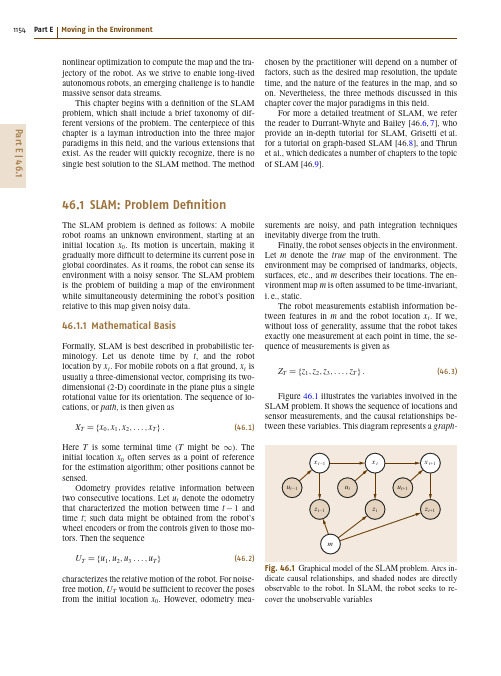
Part E|46.11154Part E Moving in the Environmentnonlinear optimization to compute the map and the tra-jectory of the robot.As we strive to enable long-lived autonomous robots,an emerging challenge is to handle massive sensor data streams.This chapter begins with a deﬁnition of the SLAM problem,which shall include a brief taxonomy of dif-ferent versions of the problem.The centerpiece of thischapter is a layman introduction into the three majorparadigms in this ﬁeld,and the various extensions that exist.As the reader will quickly recognize,there is nosingle best solution to the SLAM method.The methodchosen by the practitioner will depend on a number of factors,such as the desired map resolution,the update time,and the nature of the features in the map,and so on.Nevertheless,the three methods discussed in this chapter cover the major paradigms in this ﬁeld.For more a detailed treatment of SLAM,we refer the reader to Durrant-Whyte and Bailey [46.6,7],who provide an in-depth tutorial for SLAM,Grisetti et al.for a tutorial on graph-based SLAM [46.8],and Thrun et al.,which dedicates a number of chapters to the topic of SLAM [46.9].46.1SLAM:Problem DefinitionThe SLAM problem is deﬁned as follows:A mobile robot roams an unknown environment,starting at an initial location x 0.Its motion is uncertain,making it gradually more difﬁcult to determine its current pose in global coordinates.As it roams,the robot can sense its environment with a noisy sensor.The SLAM problem is the problem of building a map of the environment while simultaneously determining the robot’s position relative to this map given noisy data.46.1.1Mathematical BasisFormally,SLAM is best described in probabilistic ter-minology.Let us denote time by t ,and the robot location by x t .For mobile robots on a ﬂat ground,x t is usually a three-dimensional vector,comprising its two-dimensional (2-D)coordinate in the plane plus a single rotational value for its orientation.The sequence of lo-cations,or path ,is then given asX T D f x 0;x 1;x 2;:::;x T g :(46.1)Here T is some terminal time (T might be 1).The initial location x 0often serves as a point of reference for the estimation algorithm;other positions cannot be sensed.Odometry provides relative information between two consecutive locations.Let u t denote the odometry that characterized the motion between time t 1and time t ;such data might be obtained from the robot’s wheel encoders or from the controls given to those mo-tors.Then the sequenceU T D f u 1;u 2;u 3:::;u T g (46.2)characterizes the relative motion of the robot.For noise-free motion,U T would be sufﬁcient to recover the poses from the initial location x 0.However,odometry mea-surements are noisy,and path integration techniques inevitably diverge from the truth.Finally,the robot senses objects in the environment.Let m denote the true map of the environment.The environment may be comprised of landmarks,objects,surfaces,etc.,and m describes their locations.The en-vironment map m is often assumed to be time-invariant,i.e.,static.The robot measurements establish information be-tween features in m and the robot location x t .If we,without loss of generality,assume that the robot takes exactly one measurement at each point in time,the se-quence of measurements is given as Z T D f z 1;z 2;z 3;:::;z T g :(46.3)Figure 46.1illustrates the variables involved in the SLAM problem.It shows the sequence of locations and sensor measurements,and the causal relationships be-tween these variables.This diagram represents agraph-Fig.46.1Graphical model of the SLAM problem.Arcs in-dicate causal relationships,and shaded nodes are directly observable to the robot.In SLAM,the robot seeks to re-cover the unobservable variablesMultimedia Contents Simultaneou 1153Part E |4646.Simultaneous Localizationand MappingCyrill Stachniss,John J.Leonard,Sebastian Thrun This chapter provides a comprehensive intro-duction in to the simultaneous localization and mapping problem ,better known in its abbreviated form as SLAM.SLAM addresses the main percep-tion problem of a robot navigating an unknown environment.While navigating the environment,the robot seeks to acquire a map thereof,and at the same time it wishes to localize itself us-ing its map.The use of SLAM problems can be motivated in two different ways:one might be in-terested in detailed environment models,or one might seek to maintain an accurate sense of a mo-bile robot’s location.SLAM serves both of these purposes.We review the three major paradigms from which many published methods for SLAM are de-rived:(1)the extended Kalman filter (EKF);(2)particle filtering;and (3)graph optimization.We also review recent work in three-dimensional (3-D)SLAM using visual and red green blue dis-46.1SLAM:Problem Definition .....................115446.1.1Mathematical Basis ...................115446.1.2Example:SLAM in Landmark Worlds ..................115546.1.3Taxonomy of the SLAM Problem ..115646.2The Three Main SLAM Paradigms ...........115746.2.1Extended Kalman Filters ............115746.2.2Particle Methods .......................115946.2.3Graph-Based Optimization Techniques ............116246.2.4Relation of Paradigms ................116646.3Visual and RGB-D SLAM ........................116646.4Conclusion and Future Challenges .. (1169)Video-References .........................................1170References ...................................................1171tance-sensors (RGB-D),and close with a discussion of open research problems in robotic mapping.This chapter provides a comprehensive introduction into one of the key enabling technologies of mobile robot navigation:simultaneous localization and map-ping ,or in short SLAM .SLAM addresses the problem of acquiring a spatial map of an environment while si-multaneously localizing the robot relative to this model.The SLAM problem is generally regarded as one of the most important problems in the pursuit of building truly autonomous mobile robots.It is of great practical im-portance;if a robust,general-purpose solution to SLAM can be found,then many new applications of mobile robotics will become possible.While the problem is deceptively easy to state,it presents many challenges,despite signiﬁcant progress made in this area.At present,we have robust methods for mapping environments that are mainly static,struc-tured,and of limited size.Robustly mapping unstruc-tured,dynamic,and large-scale environments in an on-line fashion remains largely an open research problem.The historical roots of methods that can be applied to address the SLAM problem can be traced back to Gauss [46.1],who is largely credited for inventing the least squares method.In the Twentieth Century,a num-ber of ﬁelds outside robotics have studied the making of environment models from a moving sensor platform,most notably in photogrammetry [46.2–4]and com-puter vision [46.5].Strongly related problems in these ﬁelds are bundle adjustment and structure from mo-tion.SLAM builds on this work,often extending the basic paradigms into more scalable algorithms.Mod-ern SLAM systems often view the estimation problem as solving a sparse graph of constraints and applying。

140510雅思考试阅读考题回顾

Acriticismoftheclimateextinctionargumentisthattheworldwarmedwellbeforethecreaturesbecameextinctandsothatcouldnothavebeenthecause.
题型难度分析
第一篇的题型包括是非无判断题，表格填空以及归纳摘要填空。这篇文章是旧题，曾在2011年8月出现过，但是题型是新的题型。当年考了matching题中的人名观点搭配题，而此次的考法相对难度降低。
部分答案：
1-6TRUE/FALSE/NOTGIVEN:
1.这个人一开始就认出来这是什么残骸：TRUE
2.是人类发现的最完整的：TRUE
3.发现人的朋友懂的比他多：NOTGIVEN
表格填空：
7.象牙tusk
8.死亡原因是窒息suffocation
9.死亡时间spring,小象生在earlyspring,一个月以后就死了
剑桥雅思推荐原文练习
剑5Test2
ReadingPassage2
Title:
Comparison betweenClassicandNeoclassicOrganization
Questiontypes:
Multiplechoices（5选2）;
Matchingpeoplewithopinions;
Theyfoundthatthespeciesnearlywentextinct120,000yearsagowhentheworldwarmedupforawhile.Numbersarethoughttohavedroppedfromseveralmilliontotensofthousandsbutnumbersrecoveredastheplanetenteredanothericeage.

基于Cesium的气体扩散可视化系统

2020年软件2020, V ol. 41, No. 7作者简介: 高齐琦(1992–)，女，助理工程师，主要研究方向：数据可视化；郑凌兵(1986–)，男，工程师，主要研究方向：系统软件构建；孙涛(1982–)，男，工程师，主要研究方向：云计算、大数据、数据可视化。

基于Cesium 的气体扩散可视化系统高齐琦，郑凌兵，孙涛（中电海康集团有限公司，杭州 310000）摘要: 气体扩散是一种常见现象，搭建高效的可视化系统，对探索气体扩散规律并做出快速、准确、普适性应对具有重要意义。

本文针对目前气体扩散可视化存在的不足，提出建立基于Cesium 的气体扩散可视化系统。

系统采用B/S 架构，在服务器端采用高斯烟羽模型对气体扩散进行模拟计算，在客户端完成气体扩散可视化效果。

着重讲述了可视化效果的方法改进与过程实现，完成了使用canvas 绘制热力图并将其与Cesium 地图引擎结合的应用。

关键词: 气体扩散；可视化系统；Cesium中图分类号: TP311.52 文献标识码: A DOI ：10.3969/j.issn.1003-6970.2020.07.045本文著录格式：高齐琦，郑凌兵，孙涛. 基于Cesium 的气体扩散可视化系统[J]. 软件，2020，41（07）：220 223Visualization System of Gas Diffusion Based on CesiumGAO Qi-qi, ZHENG Ling-bing, SUN Tao(CETHIK GROUP CO., LTD, HangZhou 310000, China )【Abstract 】: Gas diffusion is a common phenomenon. Building an efficient visualization system is of great signifi-cance to explore the law of gas diffusion and make a rapid, accurate and universal response. In view of the short-comings of current visualization of gas diffusion, a gas diffusion visualization system based on Cesium is proposed in this paper. The system uses B/S architecture, and the Gauss plume model is used to simulate the gas diffusion on the server side, and the visualization of gas diffusion is completed on the client side. This paper focuses on the im-provement of visualization method and the realization of the process, and completes the application of drawing thermal map with canvas and combining it with Cesium map engine. 【Key words 】: Gas diffusion; Visualization system; Cesium0 引言国内外对气体扩散有一定的研究积累，如地铁周围气体扩散可视化[1]、海上事故有害气体的扩散研究[2]、轻量级有毒气体扩散在线可视化仿真平台[3]等，但是研究重点多集中在对扩散规律的数学模拟，借助ArcGIS 、Matlab 等软件生成图片展示计算结果，或是将分析计算与可视化都放在服务器端进行，造成服务器压力大等问题[4-5]，无法形成完整高效的可视化系统。

GammaFunction：伽玛函数

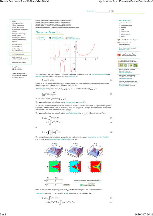
Search Site12,720 entries Calculus and Analysis > Special Functions > Gamma Functions Calculus and Analysis > Special Functions > Named Integrals Calculus and Analysis > Special Functions > Product Functions Gamma FunctionThe (complete) gamma function is defined to be an extension of the factorial to arguments. It is related to the factorial bya slightly unfortunate notation due to Legendre which is now universally used instead of Gauss's simpler (Gauss 1812; Edwards 2001, p. 8). everywhere except at, -1, -2, ..., and the residue atisThere are no points at which.There are a number of notational conventions in common use for indication of a power of a gamma functions. While authors such as Watson (1939) use (i.e., using a trigonometric function-like convention), it is also common to write . for(Euler's integral form)The complete gamma function can be generalized to the upper and lower incomplete gamma function .Min MaxRe Register for Unlimited Interactive Examples >>Im ReplotPlots of the real and imaginary parts of in the complex plane are illustrated above.Wolfram Research Demonstrations Site Integrator Tones Functions Site Wolfram Science more…Download Complete Documentation >>Find 171 formulas about the Gamma Function at -55-55(8)(9)If is an integer, 2, 3, ..., then(10)(11)so the gamma function reduces to the factorial for a positive integer argument.A beautiful relationship betweenand the Riemann zeta functionis given by(12)for(Havil 2003, p. 60).The gamma function can also be defined by an infinite product form (Weierstrass form )(13)where is the Euler-Mascheroni constant (Krantz 1999, p. 157; Havil 2003, p. 57). This can be written(14)where(15)(16)for, where is the Riemann zeta function (Finch 2003). Taking the logarithm of both sidesof (◇),(17)Differentiating,(18)(19)(20)(21)(22)(23)(24)(25)where is the digamma function and is the polygamma function . th derivatives are given in terms of the polygamma functions , , ..., .The minimum valueoffor real positiveis achieved when(26)(27)This can be solved numerically to give (Sloane's A030169; Wrench 1968), which has continued fraction [1, 2, 6, 63, 135, 1, 1, 1, 1, 4, 1, 38, ...] (Sloane's A030170). At ,achieves the value 0.8856031944... (Sloane's A030171), which has continued fraction [0, 1, 7, 1, 2, 1, 6, 1, 1, ...] (Sloane's A030172).The Euler limit form is(28)so(29)(30)(31)(32)(Krantz 1999, p. 156).One over the gamma functionis an entire function and can be expressed as(33)where is the Euler-Mascheroni constant and is the Riemann zeta function (Wrench 1968). An asymptotic series for is given by(34) Writing(35) the satisfy(36) (Bourguet 1883, Davis 1933, Isaacson and Salzer 1943, Wrench 1968). Wrench (1968) numerically computed the coefficients for the series expansion about 0 of(37) The Lanczos approximation gives a series expansion for for in terms of an arbitrary constant such that .The gamma function satisfies the functional equations(38)(39) Additional identities are(40)(41)(42)(43)Using (40), the gamma function of a rational number can be reduced to a constant times or . For example,(44)(45)(46)(47) For ,(48) Gamma functions of argument can be expressed using the Legendre duplication formula(49) Gamma functions of argument can be expressed using a triplication formula(50) The general result is the Gauss multiplication formula(51) The gamma function is also related to the Riemann zeta function by(52) For integer , 2, ..., the first few values of are 1, 1, 2, 6, 24, 120, 720, 5040, 40320, 362880, ... (Sloane's A000142). For half-integer arguments, has the special form(53)where is a double factorial. The first few values for , 3, 5, ... are therefore(54)(55)(56), , ... (Sloane's A001147 and A000079; Wells 1986, p. 40). In general, for a positive integer, 2, ...(57)(58)(59)(60) Simple closed-form expressions of this type do not appear to exist for for a positive integer . However, Borwein and Zucker (1992) give a variety of identities relating gamma functions to square roots and elliptic integral singular values, i.e., elliptic moduli such that(61)where is a complete elliptic integral of the first kind and is the complementary integral. M. Trott (pers. comm.) has developed an algorithm for automatically generating hundreds of such identities.(62)(63)(64)(65)(66)(67)(68)(69)(70)(71)(72)(73)(74)(75)(76)(77)(78)(79)(80)(81)(82)Several of these are also given in Campbell (1966, p. 31).A few curious identities include(83)(84)(85)(86)(87)(88)(89) of which Magnus and Oberhettinger 1949, p. 1 give only the last case,(90) and(91)(Magnus and Oberhettinger 1949, p. 1). Ramanujan also gave a number of fascinating identities:(92)(93) where(94)(95)(Berndt 1994).Ramanujan gave the infinite sums(96)(97) and(98)(99)(Hardy 1923; Hardy 1924; Whipple 1926; Watson 1931; Bailey 1935; Hardy 1999, p. 7).The following asymptotic series is occasionally useful in probability theory (e.g., theone-dimensional random walk):(100) (Graham et al. 1994). This series also gives a nice asymptotic generalization of Stirling numbers of the first kind to fractional values.It has long been known that is transcendental (Davis 1959), as is (Le Lionnais 1983; Borwein and Bailey 2003, p. 138), and Chudnovsky has apparently recently proved thatis itself transcendental (Borwein and Bailey 2003, p. 138).There exist efficient iterative algorithms for for all integers (Borwein and Bailey 2003, p. 137). For example, a quadratically converging iteration for (Sloane'sA068466) is given by defining(101)(102) setting and , and then(103)(Borwein and Bailey 2003, pp. 137-138).No such iteration is known for (Borwein and Borwein 1987; Borwein and Zucker 1992; Borwein and Bailey 2003, p. 138).SEE ALSO:Bailey's Theorem, Barnes G-Function, Binet's Fibonacci Number Formula, Bohr-Mollerup Theorem, Digamma Function, Double Gamma Function, Fransén-Robinson Constant Gauss Multiplication Formula, Incomplete Gamma Function, Knar's Formula, Lambda Function, LanczosApproximation, Legendre Duplication Formula, Log Gamma Function, Mellin's Formula, Mu Function, Nu Function, Pearson's Function, Polygamma Function, Regularized Gamma Function, Stirling's Series, Superfactorial. [Pages Linking Here]RELATED WOLFRAM SITES:/GammaBetaErf/Gamma/,/GammaBetaErf/LogGamma/REFERENCES:Abramowitz, M. and Stegun, I. A. (Eds.). "Gamma (Factorial) Function" and "Incomplete Gamma Function." §6.1 and 6.5 in Handbook of Mathematical Functions with Formulas, Graphs, and Mathematical Tables, 9th printing. New York: Dover, pp. 255-258 and 260-263, 1972.Arfken, G. "The Gamma Function (Factorial Function)." Ch. 10 in Mathematical Methods for Physicists, 3rd ed. Orlando, FL: Academic Press, pp. 339-341 and 539-572, 1985.Artin, E. The Gamma Function. New York: Holt, Rinehart, and Winston, 1964.Bailey, W. N. Generalised Hypergeometric Series. Cambridge, England: Cambridge University Press, 1935.Berndt, B. C. Ramanujan's Notebooks, Part IV. New York: Springer-Verlag, pp. 334-342, 1994.Beyer, W. H. CRC Standard Mathematical Tables, 28th ed. Boca Raton, FL: CRC Press, p. 218, 1987.Borwein, J. and Bailey, D. Mathematics by Experiment: Plausible Reasoning in the 21st Century. Wellesley, MA: A K Peters, 2003.Borwein, J. and Borwein, P. B. Pi & the AGM: A Study in Analytic Number Theory and Computational Complexity. New York: Wiley, p. 6, 1987.Borwein, J. M. and Zucker, I. J. "Fast Evaluation of the Gamma Function for Small Rational Fractions Using Complete Elliptic Integrals of the First Kind." IMA J. Numerical Analysis12, 519-526, 1992.Bourguet, L. "Sur les intégrales Eulériennes et quelques autres fonctions uniformes." Acta Math.2, 261-295, 1883. Campbell, R. Les intégrales eulériennes et leurs applications. Paris: Dunod, 1966.Davis, H. T. Tables of the Higher Mathematical Functions. Bloomington, IN: Principia Press, 1933.Davis, P. J. "Leonhard Euler's Integral: A Historical Profile of the Gamma Function." Amer. Math. Monthly66, 849-869, 1959.Erdélyi, A.; Magnus, W.; Oberhettinger, F.; and Tricomi, F. G. "The Gamma Function." Ch. 1 in Higher Transcendental Functions, Vol. 1. New York: Krieger, pp. 1-55, 1981.Finch, S. R. "Euler-Mascheroni Constant." §1.5 in Mathematical Constants. Cambridge, England: Cambridge University Press, pp. 28-40, 2003.Gauss, C. F. "Disquisitiones Generales Circa Seriem Infinitametc. Pars Prior." Commentationes Societiones Regiae Scientiarum Gottingensis Recentiores, Vol. II. 1812. Reprinted in Gesammelte Werke, Bd. 3, pp. 123-163 and 207-229, 1866.Graham, R. L.; Knuth, D. E.; and Patashnik, O. Answer to Problem 9.60 in Concrete Mathematics: A Foundation for Computer Science, 2nd ed. Reading, MA: Addison-Wesley, 1994.Hardy, G. H. "A Chapter from Ramanujan's Note-Book." Proc. Cambridge Philos. Soc.21, 492-503, 1923.Hardy, G. H. "Some Formulae of Ramanujan." Proc. London Math. Soc. (Records of Proceedings at Meetings) 22,xii-xiii, 1924.Hardy, G. H. Ramanujan: Twelve Lectures on Subjects Suggested by His Life and Work, 3rd ed. New York: Chelsea, 1999.Havil, J. "The Gamma Function." Ch. 6 in Gamma: Exploring Euler's Constant. Princeton, NJ: Princeton University Press, pp. 53-60, 2003.Isaacson, E. and Salzer, H. E. "Mathematical Tables--Errata: 19. J. P. L. Bourget, 'Sur les intégrales Eulériennes et quelques autres fonctions uniformes,' Acta Mathematica, v. 2, 1883, pp. 261-295.' " Math. Tab. Aids Comput.1, 124, 1943.Koepf, W. "The Gamma Function." Ch. 1 in Hypergeometric Summation: An Algorithmic Approach to Summation and Special Function Identities. Braunschweig, Germany: Vieweg, pp. 4-10, 1998.Krantz, S. G. "The Gamma and Beta Functions." §13.1 in Handbook of Complex Variables. Boston, MA: Birkhäuser, pp. 155-158, 1999.Le Lionnais, F. Les nombres remarquables. Paris: Hermann, p. 46, 1983.Magnus, W. and Oberhettinger, F. Formulas and Theorems for the Special Functions of Mathematical Physics. New York: Chelsea, 1949.Nielsen, N. "Handbuch der Theorie der Gammafunktion." Part I in Die Gammafunktion. New York: Chelsea, 1965. Press, W. H.; Flannery, B. P.; Teukolsky, S. A.; and Vetterling, W. T. "Gamma Function, Beta Function, Factorials, Binomial Coefficients" and "Incomplete Gamma Function, Error Function, Chi-Square Probability Function, Cumulative Poisson Function." §6.1 and 6.2 in Numerical Recipes in FORTRAN: The Art of Scientific Computing, 2nd ed. Cambridge, England: Cambridge University Press, pp. 206-209 and 209-214, 1992.Sloane, N. J. A. Sequences A000079/M1129, A000142/M1675, A001147/M3002, A030169, A030170, A030171,A030172, and A068466 in "The On-Line Encyclopedia of Integer Sequences."Spanier, J. and Oldham, K. B. "The Gamma Function " and "The Incomplete Gamma and Related Functions." Chs. 43 and 45 in An Atlas of Functions. Washington, DC: Hemisphere, pp. 411-421 and 435-443, 1987. Watson, G. N. "Theorems Stated by Ramanujan (XI)." J. London Math. Soc.6, 59-65, 1931.Watson, G. N. "Three Triple Integrals." Quart. J. Math., Oxford Ser. 210, 266-276, 1939.Wells, D. The Penguin Dictionary of Curious and Interesting Numbers. Middlesex, England: Penguin Books, p. 40, 1986. Whipple, F. J. W. "A Fundamental Relation between Generalised Hypergeometric Series." J. London Math. Soc.1,138-145, 1926.Whittaker, E. T. and Watson, G. N. A Course in Modern Analysis, 4th ed. Cambridge, England: Cambridge University Press, 1990.Wrench, J. W. Jr. "Concerning Two Series for the Gamma Function." Math. Comput.22, 617-626, 1968.LAST MODIFIED:December 26, 2005CITE THIS AS:Weisstein, Eric W. "Gamma Function." From MathWorld--A Wolfram Web Resource./GammaFunction.html© 1999 CRC Press LLC, © 1999-2007 Wolfram Research, Inc. | Terms of Use。

羌北地块上志留统龙木措上组岩石磁学特征

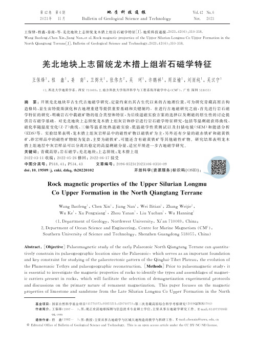
第42卷第6期2023年 11月地质科技通报B u l l e t i n o f G e o l o g i c a l S c i e n c e a n d T e c h n o l o g yV o l .42 N o .6N o v . 2023王保锋,程鑫,姜南,等.羌北地块上志留统龙木措上组岩石磁学特征[J ].地质科技通报,2023,42(6):310-318.W a n g B a o f e n g ,C h e n X i n ,J i a n g N a n ,e t a l .R o c k m a g n e t i c p r o p e r t i e s o f t h e U p p e r S i l u r i a n L o n g m u C o U p pe r F o r m a t i o n i n t h e N o r t h Q i a n g t a n g T e r r a n e [J ].B u l l e t i n of G e o l og i c a l S c i e n c e a n d T e ch n o l o g y,2023,42(6):310-318.基金项目:国家自然科学基金项目(41774073;91855211;42074075);第二次青藏高原综合科学考察研究(2019Q Z K K 0704)作者简介:王保锋(1997 ),男,现正攻读地球探测与信息技术专业硕士学位,主要从事古地磁学研究工作㊂E -m a i l :614975769@q q.c o m 通信作者:程鑫(1982 ),男,教授,主要从事古地磁学与区域大地构造的教学与科研工作㊂E -m a i l :c h e n x i n @n w u .e d u .c n©E d i t o r i a l O f f i c e o f B u l l e t i n o f G e o l o g i c a l S c i e n c e a n d T e c h n o l o g y .T h i s i s a n o pe n a c c e s s a r t i c l e u n d e r t h e C C B Y -N C -N D l i c e n s e .羌北地块上志留统龙木措上组岩石磁学特征王保锋1,程鑫1,姜南1,卫弼天1,张伟杰2,吴珂1,许鹏祥1,周亚楠1,刘雨纯1,吴汉宁1(1.西北大学地质学系,西安710069;2.南方科技大学海洋科学与工程系海洋磁学中心(C M 2),广东深圳518055)摘要:开展羌北地块早古生代古地磁学研究,定量约束出其古生代以来的古地理位置,可为研究青藏高原古构造格局㊁显生宙特提斯演化和古地理重建等提供重要基础和关键制约㊂在进行古地磁研究之前,首先进行岩石磁学特征的研究,明确岩石中载磁矿物的组合类型和特征,为后续退磁实验方案的选择以及剩磁的原生性的讨论提供岩石磁学基础㊂对羌北地块上志留统龙木措上组灰岩和砂岩进行岩石磁学特征研究,包括等温剩磁获得曲线㊁磁化率随温度变化(χ-T )曲线㊁三轴等温系统热退磁实验㊁低温磁学性质测试以及扫描电镜(S E M )和能谱分析(E D S)等㊂实验结果表明,龙木措上组灰岩样品中的磁性矿物以磁铁矿为主,另外还有少量的磁赤铁矿和磁黄铁矿,砂岩样品中的磁性矿物较为复杂,主要为磁铁矿,可能还含有磁黄铁矿等其他磁性矿物㊂研究结果表明龙木措上组地层中灰岩样品可以分离出稳定的高温剩磁分量,适宜开展进一步古地磁学研究㊂关键词:青藏高原;岩石磁学;羌北地块;上志留统;龙木措上组2022-03-11收稿;2022-05-26修回;2022-06-17接受中图分类号:P 318.41;P 534.43 文章编号:2096-8523(2023)06-0310-09d o i :10.19509/j .c n k i .d z k q.t b 20220102 开放科学(资源服务)标识码(O S I D ):R o c k m a g n e t i c p r o p e r t i e s o f t h e U p p e r S i l u r i a n L o n gm u C o U p p e r F o r m a t i o n i n t h e N o r t h Q i a n g t a n g Te r r a n e W a n g B a of e ng 1,C h e n X i n 1,J i a n g N a n 1,W e i B i t i a n 1,Z h a n g W e i ji e 2,W u K e 1,X u P e n g x i a n g 1,Z h o u Y a n a n 1,L i u Y u c h u n 1,W u H a n n i n g1(1.D e p a r t m e n t o f G e o l o g y ,N o r t h w e s t U n i v e r s i t y,X i 'a n 710069,C h i n a ;2.D e p a r t m e n t o f O c e a n S c i e n c e a n d E n g i n e e r i n g ,C e n t r e f o r M a r i n e M a g n e t i s m (C M 2),S o u t h e r n U n i v e r s i t y o f S c i e n c e a n d T e c h n o l o g y ,S h e n z h e n G u a n g d o n g 518055,C h i n a )A b s t r a c t :[O b je c t i v e ]P a l a e o m a g n e t i c s t u d y of t h e e a r l y P a l a e o z o i c N o r t h Q i a ng t a n g T e r r a n e c a n q u a n t i t a -t i v e l y c o n s t r a i n i t s p a l a e o g e o g r a phi c l o c a t i o n s i n c e t h e P a l a e o z o i c ,w h i c h s e r v e s a s a n i m po r t a n t f o u n d a t i o n a n d k e y c o n s t r a i n t f o r s t u d y i n g o f t h e p a l a e o t e c t o n i c p a t t e r n o f t h e Q i n gh a i -T i b e t P l a t e a u ,t h e e v o l u t i o n o f t h e P h a n e r o z o i c T e t h y s a n d p a l a e o g e o g r a p h i c r e c o n s t r u c t i o n .[M e t h o d s ]P r i o r t o p a l a e o m a g n e t i c s t u d y,i t i s e s s e n t i a l t o i n v e s t i g a t e t h e m a g n e t i c p r o p e r t i e s o f r o c k s t o i d e n t i f y t h e t y p e s a n d a s s e m b l a g e s o f m a gn e t -i c c a r r i e r s p r e s e n t i n r o c k s ,w h i c h w i l l f a c i l i t a t e t h e s e l e c t i o n o f d e m a g n e t i z a t i o n e x pe r i m e n t a l p r o t o c o l s a n d d i s c u s s i o n s o n t h e p r i m a r y n a t u r e of r e m a n e n t m ag n e t i z a t i o n .Thi s p a p e r f o c u s e s o n t h e m a gn e t i c p r o p e r t i e s o f l i m e s t o n e a n d s a n d s t o n e f r o m t h e L a t e S i l u r i a n L o n g m u C o U p pe r F o r m a t i o n i n t h e N o r t h第6期王保锋等:羌北地块上志留统龙木措上组岩石磁学特征Q i a n g t a n g T e r r a n e ,t h r o u g h a n a l y s e s o f i s o t h e r m a l r e m a n e n c e a c q u i s i t i o n c u r v e s ,m a g n e t i c s u s c e p t i b i l i t yw i t h t e m p e r a t u r e (χ-T )c u r v e s ,t r i a x i a l t h e r m a l d e m a g n e t i z a t i o n e x p e r i m e n t s ,l o w -t e m p e r a t u r e m a g n e t i c p r o p e r t i e s t e s t s ,s c a n n i n g e l e c t r o n m i c r o s c o p y (S E M )a n d e n e r g y d i s p e r s i v e s p e c t r a l (E D S )a n a l ys i s .[R e -s u l t s ]R e s u l t s s h o w t h a t m a g n e t i t e i s t h e p r e d o m i n a n t m a g n e t i c c a r r i e r i n t h e l i m e s t o n e s a m pl e s o f t h e L o n g m u C o U p p e r F m ,w i t h s m a l l a m o u n t s o f p y r r h o t i t e .T h e m a g n e t i c a s s e m b l a ge i n t h e s a n d s t o n e s a m -p l e s i s m o r e c o m p l e x ,d o m i n a t e d b y m a g n e t i t e ,p o s s i b l y w i t h o t h e r m a g n e t i c m i n e r a l s s u c h a s p yr r h o t i t e .[C o n c l u s i o n ]M o r e o v e r ,i t d e m o n s t r a t e s t h a t s t a b l e h i g h -t e m p e r a t u r e r e m a n e n t m a g n e t i z a t i o n c o m po n e n t s c a n b e i s o l a t e d f r o m t h e l i m e s t o n e s a m p l e s i n t h e L o n g m u C o U p p e r F o r m a t i o n ,m a k i n g t h e m s u i t a b l e f o r f u r t h e r p a l a e o m a g n e t i c r e s e a r c h e s .K e y wo r d s :Q i n g h a i -T i b e t P l a t e a u ;r o c k m a g n e t i s m ;N o r t h Q i a n g t a n g T e r r a n e ;U p p e r S i l u r i a n ;L o n g m u C o U p pe r F o r m a t i o n R e c e i v e d :2022-03-11;R e v i s e d :2022-05-26;A c c e pt e d :2022-06-17图1 羌北地块及邻区大地构造简图(a )和采样区地质简图(b)F i g .1 S i m p l i f i e d t e c t o n i c m a p o f t h e N o r t h Q i a n g t a n g T e r r a n e a n d a d j a c e n t a r e a s (a )a n d s i m p l i f i e d g e o l o g i c a l m a po f t h e s a m p l i n g ar e a (b ) 青藏高原各个块体的裂离㊁漂移㊁碰撞造山和大陆增生等地质历史过程[1-4],是研究冈瓦纳大陆与欧亚大陆的离散与汇聚㊁特提斯演化和古地理重建的重要基础和核心科学问题[5-7]㊂羌北地块位于青藏高原腹地,北部以西金乌兰-金沙江缝合带为界,与松潘-甘孜地块相邻(图1-a ),南部以龙木措-双湖缝合带为界与羌南地块相邻,被认为是研究青藏高原地质演化的重要窗口㊂目前,羌北地块在早古生代的古地理位置以及它和周缘古大陆的关系仍不清楚[8-9],羌塘中部龙木措-双湖缝合带特提斯洋的性质及演化过程仍然存在争议,早古生代和晚古生代是否是一个连续的大洋[10-11],需要利用古地磁方法定量确定羌北地块早古生代的古地理位置和运动学过程㊂开展古地磁工作首先要对岩石的载磁能力进行研究,识别出岩石中所含磁性矿物的种类,为后续退磁实验方案的选择以及剩磁原生性的讨论提供岩石磁学基础㊂目前在羌北地块,已经获得了多个晚石炭世以来的古地磁数据[12-16],但早古生代只有姜南等[17]所报道的唯一一个从灰岩中所获得的古地磁数据㊂北羌塘地块早古生代地层主要出露于块体西部的拉竹龙-龙木措地区[18-20]和东部的青泥洞-海通地区,奥陶系-志留系为碎屑岩和海相碳酸盐沉积,具有扬子板块西缘沉积建造和生物组合面貌的特点㊂笔者拟对拉竹龙-龙木措地区龙木措上组灰岩和砂岩进行系统的岩石磁学研究,包括等温剩磁(i s o t h e r m a l r e m a n e n t m a y n e t i z a t i o n ,简称I R M )及反向场退磁曲线㊁三轴等温系统热退磁实验㊁磁化率随温度变化曲线㊁低温磁学性质测试以及扫描电镜(s c a n n i n g e l e c t r o n m i c r o s c o pe ,简称S E M )和能谱分析(e n e r g y d i s p e r s i v e s pe c t r o m e t e r ,简称E D S )等㊂识别出龙木措上组地层中磁性矿物的种类㊁组合与含量等特征,为后续古地磁工作提供岩石磁学基础㊂1 区域地质概况与样品采集21世纪初,在1ʒ25万温泉幅㊁松西幅地质调查中,安徽省地调院在龙木措的北部边缘发现了完整的古生代地层,包括奥陶纪㊁志留纪以及泥盆纪3个年代的地层,而山西省地调局在托合平措幅以及113h t t p s://d z k j q b.c u g.e d u.c n地质科技通报2023年土则岗日幅的地质调查中,首先划分出了早古生代地层,在土则岗日幅㊁托和平错幅中,主要位于在羌塘西部的龙木措地区[19],志留纪地层从下到上依次划分为:下部地层为龙木措下组,主要岩性是灰岩;上部地层为龙木措上组,主要岩性是碎屑岩和灰岩㊂根据岩性和沉积环境的不同,龙木措上组又可分为下段和上段㊂这些地层剖面连续完整,化石丰富,地层年龄明确,变形和变质的程度都很小,为在北羌塘地块开展早古生代古地磁学研究提供了可能㊂选取西藏自治区阿里地区日土县龙木措北东的单面山剖面(剖面坐标:N34ʎ4',E80ʎ32.8')进行古地磁采样(图1-b)㊂剖面下段为志留系龙木措下组,底部出露不全,主要是灰青色薄中层灰岩㊁细晶白云岩及钙质页岩,龙木措下组含丰富的腕足㊁双壳㊁珊瑚及海百合茎等㊂包括珊瑚S u b s l v e o l i t e s s p.,H a l y s i t e s s p.,C a t e n i p o r a s p.等志留纪的常见分子,腕足类H i n d e l l a,S t r i c k l a n d i a,S t r i-i s p i r i f e r等是下志留统典型的化石类型,及丰富的G e i s o n o c e r a s c f.r i v a l e,O o n o x e r a s c f.a c i n a c a s, C o l u m e n a s s p.,A r i o n c e r a s s p.,A.s u b m o n i i l-f o r m,V i r g o c e r a s s p.,D a w s o n o c e r a s s p.等中志留世常见的头足类化石㊂顶部和中部龙木措上组下段呈整合接触关系㊂中部龙木措上组下段,主要是灰白色厚层石英质砾岩㊁石英砂岩㊁粉砂质泥岩㊂含腹足:S u b u l i t e s s p.,腕足:D i s c u l i n a c f.h e m i s p h a-e r i c a(S o w e r b y),H o l c o t h y r i s s p.和植物茎干化石;上部龙木措上组上段被古新统蚂蟥山组红层覆盖,其底和中部龙木措上组下段呈整合接触关系,未见顶,主要是灰黄色薄中层砾岩㊁钙质细粒岩屑石英砂岩以及一些生物碎屑灰岩㊂这2个组的化石较少,具有珊瑚㊁双壳㊁腕足类化石及植物茎干化石,但保存均较差㊂但据与下伏早-中志留世龙木措下组的整合关系推测,这套厚逾1000m的地层的时代应晚于中志留世,且区域上又被中-上泥盆统不整合所覆,故推测其时代为晚志留世[21-23]㊂根据地层出露情况,结合采样区交通情况,笔者拟选择一条出露较好,地层连续完整,变形和变质程度较弱的剖面,进行古地磁样品的采集,共设计17个采点采集砂岩和灰岩2种样品(图2),使用汽油钻机钻样,然后使用太阳罗盘测量样品产状,使用磁罗盘测定地层产状㊂2实验方法与原理将野外所采的样品加工成标准的古地磁样品(高2.2c m,直径2.54c m的圆柱体),然后选取灰岩和砂岩2种不同岩性的样品,进行等温剩磁图2龙木措上组地层柱状图和野外露头照片F i g.2 S t r a t i g r a p h i c c o l u m n a n d f i e l d o u t c r o p p h o t o-g r a p h s o f t h e L o n g m u C o U p p e r F o r m a t i o n (I R M)获得及反向场退磁实验㊁三轴等温热退磁实验㊁磁化率随温度变化(χ-T)曲线㊁低温磁学性质测试以及扫描电镜(S E M)和能谱分析(E D S)㊂采用逐步热退磁(t h e r m a l d e m a y n e t i z a t i o n,简称T D)和交变退磁(a l t e r n a t i n g f i e l d,简称A F)2种退磁方法来对样品的剩磁进行清洗和分离㊂以上实验在西北大学大陆动力学国家重点实验室和中国科学院地球环境研究所完成㊂2.1等温剩磁(I R M)获得及反向场退磁实验该曲线是将岩石样品在室温下逐步加场测量得到的,先测量样品的天然剩磁(n a t u r a l r e m a n e n t m a g n e t i z a t i o n,简称N R M),然后利用A S C-I M-10-30脉冲磁力仪对样品从1m T逐步加场至2500 m T,正向场加完后加反向场退磁,每次加场后用J R-6A旋转磁力仪测试其磁化强度㊂根据矫顽力的不同,磁性矿物可以分为硬(高矫顽力)磁矿物和软(低矫顽力)磁矿物,硬磁矿物主要有赤铁矿和针铁矿等,软磁矿物主要有磁铁矿㊁磁黄铁㊁矿磁赤铁和矿胶黄铁矿等㊂在外场加到200m T时,软磁矿物213第6期王保锋等:羌北地块上志留统龙木措上组岩石磁学特征基本上趋于饱和,但硬磁矿物在2500m T时仍然难以达到饱和㊂K r u i v e r等[24]和S t o c k h a u s e n[25]提出,已经获得的等温剩磁(I R M)曲线可以用累计对数高斯(c u-m u l a t i v e l o y-G a u s s-i a n,简称C L G)曲线进行分析㊂利用该曲线可以分析磁性矿物的矫顽力谱㊁样品中磁性矿物的种类以及定量的描述不同组分所占的比例[26],如果样品中的矫顽力差别较大,或者矫顽力有重叠的部分不好分离时,可以将累计对数高斯曲线分解为I R M线性获得曲线(l i n e a r a c q u i s i t i o n p l o t,简称L A P)㊁梯度获得曲线(g r a d i e n t o f a c q u i-s i t i o n p l o t,简称G A P)以及标准化获得曲线(s t a n d-a r d i z e d a c q u i s i t i o n p l o t,简称S A P)来进行分析㊂但是利用等温剩磁(I R M)获得曲线及反向场退磁曲线只能判断出载磁矿物是软磁性还是硬磁性,还需结合三轴等温热退磁实验及磁化率随温度变化实验等,才能确定出样品中的磁性矿物㊂2.2三轴等温热退磁曲线主要是根据不同磁性矿物具有不同的矫顽力谱和解阻温度㊂利用A S C-I M-10-30脉冲磁力仪依次在样品Z㊁Y㊁X3个相互垂直的轴分别施加2.5T (强场)㊁0.4T(中场)㊁0.1T(弱场)的外场,获得3种等温剩磁(I R M),即硬磁㊁中间磁㊁软磁㊂然后用T D-48热退磁炉对样品进行系统热退磁,每次加温后利用J R-6A旋转磁力仪进行剩磁测量㊂最后根据不同磁化组分的最大解阻温度,来判别磁性矿物的类型㊂2.3磁化率随温度变化曲线(χ-T曲线)磁性矿物的种类不同,其磁化率随温度的变化表现出的特征也不同[27],利用χ-T曲线可以判断磁性矿物的种类以及颗粒大小[28]㊂磁化率随温度变化实验所使用的仪器为M F K2-F A型卡帕桥多频磁化率,将样品从室温开始一直加热到700ħ,然后冷却到40ħ,加热和冷却过程中,仪器会自动测量其在该温度点所对应的磁化率,该实验在氩气环境中完成,主要是为了降低加热过程中磁性矿物的氧化反应[29]㊂磁性矿物在加热至其居里温度附近时磁化率会急剧上升后快速下降并趋近于0,这一现象也被称为H o p k i n s o n效应[30]㊂不同磁性矿物颗粒在加热时磁化率变化形态不尽相同,如果磁化率随温度变化曲线出现了较为明显的H o p k i n s o n峰,这可能是样品中所含磁性矿物的粒径较小导致的,因为粒径较大的磁性矿物颗,通常很难观察到明显的H o p-k i n s o n峰[31]㊂2.4低温磁学性质测试某些磁性矿物的磁学性质会随着温度的降低发生转变,如磁铁矿在120K左右时发生大程度的退磁,称为V e r w e y转换[32];单斜磁黄铁矿剩磁冷却曲线在30~34K左右会出现一个突然降低[33]㊂由于磁性矿物低温转变的温度点不同,还可以区分出混合磁性矿物组合中的单个成分,因此低温曲线适用于样品中存在热不稳定的磁性矿物或含有多种磁性矿物的样品㊂取约0.1g粉末状样品装入胶囊,然后将样品冷却至2K,若在零场状态下冷却至2K时,再对样品施加5T外场,使样品在低温下获得饱和等温剩磁(s a t u r a t i o n i s o t h e r m a l r e m a n e n t m a g n e t i s a t i o n,简称S I R M),然后去掉外场,在零场中测量S I R M 随温度升高变化曲线,得到零场冷(z e r o f i e l d c o o l-i n g,简称Z F C)曲线㊂若在强场状态(5T)下冷却至2K时将外场去掉,样品获得S I R M,然后在零场中测量S I R M随温度升高变化曲线,得到场冷(f i e l dc o o l i n g,简称F C)曲线㊂2.5扫描电镜(S E M)和能谱分析(E D S)通过扫描电镜(S E M)可以在镜下观察到样品中磁性矿物的形态,能谱分析(E D S)可以分析磁性矿物的元素组成,将样品固定在载玻片上打磨至厚度在0.50~0.55mm之间,用抛光液抛光后烘干,实验前对样品表面喷炭处理确保其导电性,然后在20k V的加速电压与4.80mm的工作距离下,用T h e r m o-S c i e n t i f i c H e l i o s G4U C型聚焦离子双束显微镜观察其详细显微结构,随后用牛津电制冷能谱仪获取元素组成㊂3实验结果3.1等温剩磁(I R M)获得曲线及反向场退磁曲线通过灰岩样品的I R M曲线(图3-a,d)可以看出,随着外加场强度的增加,I R M曲线迅速爬升,样品在300m T时获得了最大剩磁强度的70%~80%左右,且在加到最大外场2500m T时仍未达到饱和,表明样品中同时存在低矫顽力和高矫顽力的磁性矿物㊂从C L G模型I R M线性获得L A P曲线(图3-b,e)和梯度获得G A P曲线(图3-c,f)的结果中得出存在2个组分,砂岩样品中以低矫顽力组分为主,所有样品低矫顽力组分的剩磁矫顽力均小于100 m T,高矫顽力组分的含量较少,其剩磁矫顽力均大于1200m T㊂样品的S-r a t i o(-I R M-0.3T/I R M)值分别为0.768和0.847,S-r a t i o的值越大,则说明低矫顽力的组分含量更高㊂综合判断可知,灰岩样品中以低矫顽力磁性矿物为主,同时还含有一些的高矫顽力磁性矿物㊂通过砂岩样品的I R M曲线(图3-g,j)可以看出,313h t t p s ://d z k j q b .c u g.e d u .c n 地质科技通报2023年图3 龙木措上组灰岩(a ~f )和砂岩(g~l )样品等温剩磁及反向场退磁曲线㊁累计高斯模型获得曲线F i g .3 A c q u i s i t i o n c u r v e s o f i s o t h e r m a l r e m a n e n t m a g n e t i z a t i o n (I R M ),b a c k -f i e l d d e m a gn e t i z a t i o n c u r v e s o f I R M a n d c u -m u l a t i v e l o g G a u s s i a n a n a l y s i s c u r v e s f o r t h e l i m e s t o n e (a -f )a n d s a n d s t o n e (g -l )s a m p l e s f r o m t h e L o n g m u C o U p-pe r F o r m a t i o n 砂岩样品的I R M 曲线在300m T 前迅速爬升并且达到饱和,表明砂岩样品中主要以中低矫顽力的磁性矿物为主㊂L A P 曲线(图3-h ,k )和G A P 曲线(图3-i ,l)表明其同样存在2个组分,以低矫顽力组分为主,剩磁矫顽力小于100m T ㊂样品的S -r a t i o (-I R M -0.3T /I R M )值分别为0.919,0.867,高矫顽力组分的剩磁矫顽力差别较大,说明砂岩样品的磁性矿物的种类较为复杂㊂3.2三轴等温热退磁曲线灰岩样品的三轴等温剩磁系统热退磁曲线(图4-a ~d )表明,灰岩样品中软磁和中间磁占主导组分,软磁㊁中间磁组分在450~500ħ时已完全解阻,可能代表了磁铁矿和铁的硫化物存在㊂硬磁组分在580~620ħ完全解阻,可能指示了磁赤铁矿的存在㊂砂岩样品的三轴等温剩磁系统热退磁曲线(图4-e ,f)表明砂岩样品中同样也是软磁组分占主导成分,硬磁和中间磁含量较少,各组分在450ħ之前磁化强度迅速衰减,最终在580ħ完全解阻,应该是矫顽力低的磁铁矿㊂3.3磁化率随温度变化曲线(χ-T 曲线)灰岩样品磁化率随温度变化曲线(χ-T 曲线)可以看出,样品的冷却曲线都在升温曲线之上,样品的初始磁化率都比较低,但冷却后的磁化率和样品的初始磁化率相差都比较大,表明在加热过程中产生的大量磁铁矿,可能是由于氩气环境中少量铁硅酸413第6期王保锋等:羌北地块上志留统龙木措上组岩石磁学特征图4 龙木措上组灰岩(a ~d )和砂岩(e ,f)样品三轴等温剩磁系统热退磁曲线F i g .4 T h e r m a l d e m a g n e t i z a t i o n o f t h r e e -a x i s I R M f o r l i m e s t o n e (a -d )a n d s a n d s t o n e (e ,f )s a m p l e s f r o m t h e L o n g-m u C o U p pe r F o r m a t i on 图5 龙木措上组灰岩(a ~d )和砂岩(e ,f )样品磁化率随温度变化(χ-T )曲线F i g .5 χ-T c u r v e s f o r l i m e s t o n e (a -d )a n d s a n d s t o n e (e ,f )s a m p l e s f r o m t h e L o n g m u C o U p pe r F o r m a t i o n 盐和磁赤铁矿㊁赤铁矿等被还原为磁铁矿所致㊂升温曲线在0~400ħ处于下降状态,在400~600ħ出现明显的峰值,可能是H o p k i n s o n 峰的存在,表明了样品中含有磁铁矿,或者是由于含F e 黏土矿物或铁硫化物的热分解造成的[34](图5-a ~d)㊂砂岩样品的冷却曲线同样高于升温曲线,冷却后的磁化率明显大于样品的初始磁化率,表明了在加热过程中有磁铁矿的产生㊂升温曲线在0~450ħ处于下降状态,在500~600ħ出现一定的峰值,说明在所测样品中均有顺磁性矿物的存在,并且在500ħ以后有磁性矿物的相变发生,在温度到达580ħ后,磁化率数值有明显下降,这可能是在实验过程中,磁性矿物发生了相变,产生了新的磁铁矿㊂冷却曲线350ħ附近出现了明显峰值,表明磁黄铁矿存在的可能(图5-e ,f)㊂3.4扫描电镜(S E M )和能谱分析(E D S )以及低温磁学性质测试为进一步确定灰岩样品中的磁性矿物,对灰岩样品进行了扫描电镜(S E M )和能谱分析(E D S )以及低温磁学性质测试㊂扫描电镜观察和能谱分析显513h t t p s ://d z k j q b .c u g.e d u .c n 地质科技通报2023年示,龙木措上组灰岩样品中的主要磁性矿物为铁氧化物(图6-a ,b ),大多数铁氧化物呈自形或半自形,直径介于2.0~5.0μm 之间,同时还含有一些铁的硫化物(图6-c),同样呈自形或半自形,直径介于2.0~4.0μm 之间㊂灰岩样品的Z F C 和F C 磁化强度随温度变化及其一阶导数曲线显示(图7),在0~50K ,样品的磁化强度随温度的升高而迅速升高,在50K 开始出现下降的趋势㊂从Z F C 曲线看,灰岩样品中可能存在磁赤铁矿[35],刚好对应了三轴等温热退磁实验中图6 龙木措上组灰岩样品扫描电镜与能谱分析图F i g .6 S c a n n i n g e l e c t r o n m i c r o s c o p e i m a g e s a n d e n e r g y d i s p e r s i v e s p e c t r a o f t h e l i m e s t o n e s a m pl e s f r o m t h e L o n g m u C o U p pe r F o r m a t i on 图7 灰岩样品的Z F C 和F C 磁化强度随温度变化曲线F i g .7 F i e l d -c o o l e d (F C )a n d z e r o -f i e l d -c o o l e d (Z F C )h e a t i n g cu r v e s o f R T S I R M o f l i m e s t o n e s a m -p l e s f r o m t h e L o n g m u C o U p pe r F o r m a t i o n 在600~620ħ解阻的硬磁组分㊂通过低温实验无法直接观察到磁铁矿的存在,可能是由于灰岩样品的磁性太弱导致的㊂3.5退磁特征灰岩样品通过热退磁和交变退磁都获得了较为稳定的特征剩磁分量,结果较为理想,样品退磁曲线具有单分量或双分量的特征,通过强度衰减曲线可以看出,灰岩样品在580ħ(70m T )时,其强度基本已衰减为0,曲线趋于原点,这和三轴等温热退磁实验的结果基本上是一致的,都表明了灰岩样品中主要的磁性矿物是磁铁矿,且磁铁矿很有可能记录了原生剩磁的方向(图8-a ,b)㊂砂岩样品的热退磁结果不太理想,虽然其天然剩磁(N R M )远大于灰岩样品的天然剩磁,但通过强度衰减曲线可以看出砂岩样品在400ħ,其强度已经衰减为N R M 的10%,在400ħ以后其退磁曲线方向已经紊乱,无法获得高温段的特征剩磁分量(图8-c ,d )㊂4 结论(1)龙木措上组灰岩样品中的载磁矿物和砂岩样品明显不同,灰岩样品中的磁性矿物以磁铁矿为主,还存在着磁赤铁矿和少量的磁黄铁矿,不同样品中磁黄铁矿的占比不同㊂砂岩样品中的磁性矿物类型较为复杂,主要为磁铁矿,还可能含有磁黄铁矿等其他磁性矿物㊂613第6期王保锋等:羌北地块上志留统龙木措上组岩石磁学特征N R M 为天然剩磁强度;实心㊁空心点分别代表正㊁负半球的投影图8 龙木措上组灰岩(a ,b )和砂岩(c ,d)样品退磁结果F i g .8 D e m a g n e t i z a t i o n r e s u l t f o r l i m e s t o n e (a ,b )a n d s a n d s t o n e (c ,d )s a m p l e s f r o m t h e L o n g m u C o U p pe r F o r m a t i o n (2)从退磁曲线来看,灰岩样品在热退磁和混合退磁过程中获得了高温段特征剩磁分量方向,很有可能是原生剩磁的方向,适合开展进一步古地磁研究㊂而砂岩样品的剩磁强度衰减较快,当温度到达400ħ时,强度已衰减为N R M 的10%,其退磁曲线轨迹已经紊乱,无法分离出高温剩磁分量㊂(所有作者声明不存在利益冲突)参考文献:[1] H o u Z ,Y a n g Z ,L u Y ,e t a l .A g e n e t i c l i n k a ge b e t w e e n s u b d u c -t i o n -a n d c o l l i s i o n -r e l a t e d p o r p h y r y C u d e p o s i t s i n c o n t i n e n t a l c o l l i s i o n z o n e s [J ].G e o l o g y,2015,43(3):247-250.[2] 王成善,郑和荣,冉波,等.活动古地理重建的实践与思考:以青藏特提斯为例[J ].沉积学报,2010,28(5):849-860.W a n g C S ,Z h e n g H R ,R a n B ,e t a l .O n p a l e o g e o g r a ph i c r e c o n -s t r u c t i o n ,a n e x a m p l e f o r a p p l i c a t i o n i n T i b e t a n T e t h y s [J ].A c -t a S e d m e n t o l o gi c a S i n i c a ,2010,28(5):849-860(i n C h i n e s e w i t h E n gl i s h a b s t r a c t ).[3] 莫宣学,潘桂堂.从特提斯到青藏高原形成:构造-岩浆时间的约束[J ].地学前缘,2006,13(6):43-51.M o X X ,P a n G T.F r o m t h e T e t h y s t o f o r m a t i o n o f t h e Q i n g-h a i -T i b e t P l a t e :C o n s t r a i n e d b y t e c t o n o -m a g n a t i c e v e n t s [J ].E a r t h S c i e n c e F r o n t i e r s ,2006,13(6):43-51(i n C h i n e s e w i t h E n gl i s h a b s t r a c t ).[4] Y i n A ,H a r r i s o n T M.G e o l o g i c e v o l u t i o n o f t h e H i m a l a ya n -T i -b e t a n o r o g e n [J ].A n n u a l R e v i e w o f E a r t h &P l a n e t a r y Sc i -e n c e s ,2003,28:211-280.[5] 李德威,庄育勋.青藏高原大陆动力学的科学问题[J ].地质科技情报,2006,26(2):1-10,18.L i D W ,Z h u a n g Y X.S c i e n t i f i c p r o b l e m s o f c o n t i n e n t a l d yn a m -i c s i n t h e Q i n g h a i -T i b e t P l a t e a u [J ].G e o l o g i c a l S c i e n c e a n d T e c h n o l o g yI n f o r m a t i o n ,2006,26(2):1-10,18(i n C h i n e s e w i t h E n gl i s h a b s t r a c t ).[6] 吴福元,黄宝春,叶凯,等.青藏高原造山带的垮塌与高原隆升[J ].岩石学报,2008,24(1):1-30.W u F Y ,H u a n g B C ,Y e K ,e t a l .C o l l a p s e d H i m a l a ya n -T ib e t a n o r o g e n y a n d t h e r i s i n g T i b e t a n P l a t e a u [J ].Ac t a P e t r o l o gi c a S i n i c a ,2008,24(1):1-30(i n C h i n e s e w i t h E n g l i s h a b s t r a c t ).[7] 许志琴,杨经绥,李文昌,等.青藏高原中的古特提斯体制与增生造山作用[J ].岩石学报,2013,29(6):1847-1860.X u Z Q ,Y a n g J S ,L i W C ,e t a l .P a l e o -T e t h y s s ys t e m a n d a c c r e -t i o n a r y o r o g e n y i n t h e T i b e t P l a t e a u [J ].A c t a P e t r o l o g i c a S i n i c a ,2013,29(6):1847-1860(i n C h i n e s e w i t h E n gl i s h a b s t r a c t ).[8] 谭富文,王剑,付修根,等.藏北羌塘盆地基底变质岩的锆石S H R I M P 年龄及其地质意义[J ].岩石学报,2009,25(1):139-146.T a n F W ,W a n g J ,F u X G ,e t a l .U -P b z i r c o n S H R I M P a ge of m e t -a m o r p h i c r o c k s f r o m t h e b a s e m e n t o f t h e Q i a ng t a n g Ba s i n ,n o r t h -e r n T ib e t ,a n d i t s g e o l o g ic a l s i g n i f i c a n c e [J ].A c t a P e t r o l o gi c a S i n i -c a ,2009,25(1):139-146(i n C h i n e s e w i t h E n gl i s h a b s t r a c t ).[9] 卢占武,高锐,李永铁.青藏高原羌塘盆地基底结构与南北向变化:基于一条270k m 反射地震剖面的认识[J ].岩石学报,2011,27(11):3319-3327.L u Z W ,G a o R ,L i Y T .S t r u c t u r e o f b a s e m e n t a n d i t s N -S d i r e c -t i o n t r a n s f o r m a t i o n i n Q i a n g t a n g B a s i n i n T i b e t :D i s c o v e r e d b y a270k m s e i s m i c r e f l e c t i o n p r o f i l e [J ].A t c a P e t r o l o g i c a S i n i c a ,2011,27(11):3319-3327(i n C h i n e s e w i t h E n gl i s h a b s t r a c t ).[10]胡培远,李才,吴彦旺,等.藏北羌塘中部存在志留纪洋盆:来自桃形湖蛇绿岩中斜长花岗岩的锆石U -P b 年龄证据[J ].地质通报,2014,33(11):1651-1661.H u P Y ,L i C ,W u Y W ,e t a l .T h e S i l u r i a n T e t h ya n O c e a n i n c e n t r a l Q i a n g t a n g,n o r t h e r n T i b e t :C o n s t r a i n t s f r o m z i r c o n U -P b a g e s o f p l a g i o g r a n i t e s w i t h i n t h e T a o x i n g h u o p h i o l i t e [J ].G e o l o gi c a l B u l l e t i n o f C h i n a ,2014,33(11):1651-1661(i n C h i -n e s e w i t h E n gl i s h a b s t r a c t ).[11]李三忠,赵淑娟,李玺瑶,等.东亚原特提斯洋(Ⅰ):南北边界和俯冲极性[J ].岩石学报,2016,32(9):2609-2627.L i S Z ,Z h a o S J ,L i X Y ,e t a l .P r o t o -T e h t ys O c e a n i n E a s t A -713h t t p s://d z k j q b.c u g.e d u.c n地质科技通报2023年s i a(Ⅰ):N o r t h e r n a n d s o u t h e r n b o r d e r f a u l t s a n d s u b d u c t i o n p o l a r i t y[J].A c t a P e t r o l o g i c a S i n i c a,2016,32(9):2609-2627(i nC h i n e s e w i t h E n g l i s h a b s t r a c t).[12]H u a n g K,O p d y k e N D,P e n g X J,e t a l.P a l e o m a g n e t i c r e s u l t sf r o m t h e U p p e r P e r m i a n o f t h e e a s t e r n Q i a ng t a n g T e r r a n e o fT i b e t a n d t h e i r t e c t o n i c i m p l i c a t i o n s[J].E a r t h a n d P l a n e t a r y S c i e n c e L e t t e r s,1992,111(1):1-10.[13]C h e n g X,W u H N,G u o Q,e t a l.P a l e o m a g n e t i c r e s u l t s o f L a t eP a l e o z o i c r o c k s f r o m n o r t h e r n Q i a n g t a n g B l o c k i n Q i n g h a i-T i-b e t P l a t e a u,C h i n a[J].Sc i e n c e C h i n a:E a r t h S c i e n c e s,2012,55(1):67-75.[14]C h e n g X,W u H N,D i a o Z B,e t a l.P a l e o m a g n e t i c d a t a f r o m t h eL a t e C a r b o n i f e r o u s-L a t e P e r m i a n r o c k s i n e a s t e r n T i b e t a n d t h e i r i m p l i c a t i o n s f o r t e c t o n i c e v o l u t i o n o f t h e n o r t h e r n Q i a n g-t a n g-Q a m d o b l o c k[J].S c i e n c e C h i n a:E a r t h S c i e n c e s,2013,56(7):1209-1220.[15]S o n g P P,D i n g L,L i Z Y,e t a l.A n e a r l y b i r d f r o m G o n d w a n a:P a l e o m a g n e t i s m o f L o w e r P e r m i a n l a v a s f r o m n o r t h e r n Q i a n g-t a n g(T i b e t)a n d t h e g e o g r a p h y o f t h e P a l e o-T e t h y s[J].E a r t ha n d P l a n e t a r y S c i e n c e L e t t e r s,2017,475:119-133.[16]Y a n g X F,C h e n g X,Z h o u Y N,e t a l.P a l e o m a g n e t i c r e s u l t s f r o mL a t e C a r b o n i f e r o u s t o E a r l y P e r m i a n r o c k s i n t h e n o r t h e r n Q i a n g-t a n g T e r r a n e,T i b e t,C h i n a,a n d t h e i r t e c t o n i c i m p l i c a t i o n s[J].S c i-e n c e C h i n a:E a r t h S c i e n c e s,2017,60(1):124-134.[17]姜南,吴汉宁,李玉玉,等.羌北地块早-中志留世古地磁学初步研究结果及其构造意义[J].地球物理学报,2022,65(3): 1057-1070.J i a n g N,W u H N,L i Y Y,e t a l.P r e l i m i n a r y P a l e o m a g n e t i c r e-s u l t s o f E a r l y-M i d d l e S i l u r i a n r o c k s f r o m N o r t h Q i a n g t a n g T e r r a n e,T i b e t,C h i n a,a n d i t s t e c t o n i c i m p l i c a t i o n s[J].C h i n e s e J o u r n a l o f G e o p h y s i c s,2022,65(3):1057-1070(i n C h i n e s e w i t hE n g l i s h a b s t r a c t).[18]王权,董挨管,段春森,等.西藏北部拉竹龙地区泥盆纪岩石地层单位划分与时代讨论[J].沉积与特提斯地质,2004,24(3):30-37.W a n g Q,D o n g A G,D u a n C S,e t a l.D i v i s i o n a n d a g e s o f t h eD e v o n i a n l i t h o s t r a t i g r a p h i c u n i t s i n L a z h u g l u n g,n o r t h e r n X i-z a n g[J].S e d i m e n t a r y G e o l o g y a n d T e t h y a n G e o l o g y,2004,24(3):30-37(i n C h i n e s e w i t h E n g l i s h a b s t r a c t). [19]夏军,钟华明,童劲松,等.藏北龙木错东部三岔口地区下奥陶统与泥盆系的不整合界面[J].地质通报,2006,25(1/2):113-117.X i a J,Z h o n g H M,T o n g J S,e t a l.U n c o n f o r m i t y b e t w e e n t h e L o w e r O r d v i c i a n a n d D e v o n i a n i n t h e S a n c h a k o u a r e a i n t h ee a s t e r n p a r t of t h e L u ng m u C o,n o r th e r n Ti b e t,C h i n a[J].G e o-l o g i c a l B u l l e t i n o f C h i n a,2006,25(1/2):113-117(i n C h i n e s e w i t h E n g l i s h a b s t r a c t).[20]夏军,钟华明,童劲松,等.藏西北三岔口地区泥盆系生物礁特征及其意义[J].沉积与特提斯地质,2006,26(2):34-41.X i a J,Z h o n g H M,T o n g J S,e t a l.T h e D e v o n i a n b i o h e r m s i n S a n c h a k o u,n o r t h w e s t e r n X i z a n g a n d t h e i r i m p l i c a t i o n s[J].S e d i m e n t a r y G e o l o g y a n d T e t h y a n G e o l o g y,2006,26(2):34-41(i n C h i n e s e w i t h E n g l i s h a b s t r a c t).[21]夏军,王陆太,钟华明,等.青藏高原龙木错地区志留纪大型古三角洲沉积体系的识别及其意义[J].地质通报,2009,28(9): 1267-1275.X i a J,W a n g L T,Z h o n g H M,e t a l.D i s c o v e r y o f l a r g e-s c a l e S i-l u r i a n a n c i e n t d e l t a d e p o s i t i o n s y s t e m i n L o n g m u C o a r e a, Q i n g h a i-T i b e t P l a t e a u,C h i n a a n d i t s s i g n i f i c a n c e[J].G e o l o g i c a lB u l l e t i n o fC h i n a,2009,28(9):1267-1275(i n C h i n e s e w i t hE n g l i s h a b s t r a c t).[22]G r a d s t e i n F M,O g g G,S c h m i t z M.T h e g e o l o g i c t i m e s c a l e[J].N e w s l e t t e r s o n S t r a t i g r a p h y,2012,45(2):171-188. [23]戎嘉余,王怿,詹仁斌,等.中国志留纪综合地层和时间框架[J].中国科学:地球科学,2019,49(1):93-114.R o n g J Y,W a n g Y,Z h a n R B,e t a l.S i l u r i a n i n t e g r a t i v e s t r a t i g-r a p h y a n d t i m e s c a l e o f C h i n a[J].S c i e n c e S i n i c a:E a r t h S c i-e n c e s,2019,49(1):93-114(i n C h i n e s e w i t h E n g l i s h a b s t r a c t).[24]K r u i v e r P P,D e k k e r s M J,H e s l o p D.Q u a n t i f i c a t i o n o f m a g n e t-i c c o e r c i v i t y c o m p o n e n t s b y t h e a n a l y s i s o f a c q u i s i t i o n c u r v e s o fi s o t h e r m a l r e m a n e n t m a g n e t i z a t i o n[J].E a r t h a n d P l a n e t a r yS c i e n c e L e t t e r s,2001,189(3/4):269-276.[25]S t o c k h a u s e n H.S o m e n e w a s p e c t s f o r t h e m o d e l l i n g o f i s o t h e r-m a l r e m a n e n t m a g n e t i z a t i o n a c q u i s i t i o n c u r v e s b y c u m u l a t i v e l o g G a u s s i a n f u n c t i o n s[J].G e o p h y s i c a l R e s e a r c h L e t t e r s, 1998,25(12):2217-2220.[26]K r u i v e r P P,P a s s i e r H F.C o e r c i v i t y a n a l y s i s o f m a g n e t i c p h a-s e s i n s a p r o p e l S1r e l a t e d t o v a r i a t i o n s i n r e d o x c o n d i t i o n s,i n-c l ud i n g a n i n ve s t i g a t i o n of t h e S r a t i o[J].G e o c h e m i s t r y,G e o-p h y s i c s,G e o s y s t e m s,2001,2:2001G C000181.[27]H r o u d a F.A t e c h n i q u e f o r t h e m e a s u r e m e n t o f t h e r m a l c h a n-g e s o f m a g n e t i c s u s c e p t i b i l i t y o f w e a k l y m a g n e t i c r o c k s b y t h eC S-2a p p a r a t u s a n d K L Y-2K a p p a b r i d g e[J].G e o p h y s i c a l J o u r-n a l I n t e r n a t i o n,1994,118(3):604-612.[28]V a n V A J,D e k k e r s M J.T h e i n c o r p o r a t i o n o f t h e r m a l m e t h-o d s i n m i n e r a l m a g n e t i s m o f l o e s s-p a l e o s o l s e q u e n c e:A b r i e f o v e r i e w[J].C h i n e s e S c i e n c e B u l l e t i n,1999,44:53-63. [29]李波,石显耀,李学杰,等.西菲律宾海西部沉积物磁学特征及其环境意义[J].地质科技情报,2016,35(5):34-41.L i B,S h i X Y,L i X J,e t a l.M a g n e t i c p r o p e r t i e s o f s e d i m e n t sf r o m t h e w e s t e r n W e s t P h i l i p p i n e S e a a n d t h e i r e n v i r o n m e n t a li m p l i c a t i o n s[J].G e o l o g i c a l S c i e n c e a n d T e c h n o l o g y I n f o r m a-t i o n,2016,35(5):34-41(i n C h i n e s e w i t h E n g l i s h a b s t r a c t).[30]H o p k i n s o n J.M a g n e t i c a n d o t h e r p h y s i c a l p r o p e r t i e s o f i r o n a ta h i g h t e m p e r a t u r e[J].P h i l o s o p h i c a l T r a n s a c t i o n s o f t h e R o y a lS o c i e t y o f L o n d o n.A,1889,180:443-465.[31]敖红,邓成龙.磁性矿物的磁学鉴别方法回顾[J].地球物理学进展,2007,22(2):432-442.A o H,D e n g C L.R e v i e w i n t h e i d e n t i f i c a t i o n o f m a g n e t i c m i n-e r a l s[J].P r o g r e s s i n g e o p h y s i c s,2007,22(2):432-442(i n C h i-n e s e w i t h E n g l i s h a b s t r a c t).[32]V e r w e y E J W.E l e c t r o n i c c o n d u c t i o n o f m a g n e t i t e(F e3O4)a n di t s t r a n s i t i o n p o i n t a t l o w t e m p e r a t u r e s[J].N a t u r e,1939,144(3642):327-328.[33]R o c h e t t e P,Gér a r d F i l l i o n,J e a n-L u c M a t téi,e t a l.M a g n e t i ct r a n s i t i o n a t30-34K e l v i n i n p y r r h o t i t e:I n s i g h t i n t o a w i d e-s p r e a d o c c u r r e n c e o f t h i s m i n e r a l i n r o c k s[J].E a r t h a n d P l a n-e t a r y S c i e n c e L e t t e r s,1990,98(3/4):319-328.[34]A u b o u r g C,P o z z i J P,K a r s M.B u r i a l,c l a y s t o n e s r e m a g n e t i z a-t i o n a n d s o m e c o n s e q u e n c e s f o r m a g n e t o s t r a t i g r a p h y[J].G e o-l o g i c a l S o c i e t y,L o n d o n,S p e c i a l P u b l i c a t i o n s,2012,371(1): 181-188.[35]B r u c e M M,R i c h a r d B F,S a r a h A W,e t a l.D e t e r m i n a t i o n o ft h e p r e e x p o n e n t i a l f r e q u e n c y f a c t o r f o r s u p e r p a r a m a g n e t i c m a g h e m i t e p a r t i c l e s i n m a g n e t o f e r r i t i n[J].J o u r n a l o f G e o-p h y s i c a l R e s e a r c h:S o l i d E a r t h,1997,102(B10):2671-2680.813。

Mating Siegel Quadratic Polynomials

The ﬁrst author was partially supported by NSF grant DMS-9804606. S8 July 1998
2
MICHAEL YAMPOLSKY, SAEED ZAKERI
These B¨ ottcher maps conjugate the polynomials to the squaring map: C
Contents 1. Introduction 2. Background Material 3. The Blaschke Model For Petersen’s Theorem 4. A Blaschke Model For Mating 5. Construction of Puzzle-Pieces 6. Complex Bounds 7. The Proof 8. Concluding Remarks References 1 8 12 20 27 31 40 49 53
MATING SIEGEL QUADRATIC POLYNOMIALS
arXiv:math/9808009v1 [math.DS] 3 Aug 1998
MICHAEL YAMPOLSKY, SAEED ZAKERI Abstract. Let F be a quadratic rational map of the sphere which has two ﬁxed Siegel disks with bounded type rotation numbers θ and ν . Using a new degree 3 Blaschke product model for the dynamics of F and an adaptation of complex a priori bounds for renormalization of critical circle maps, we prove that F can be realized as the mating of two Siegel quadratic polynomials with the corresponding rotation numbers θ and ν .

On the Powers of a Matrix with

3
Throughout this paper the j th column of the identity matrix will be denoted by ej . In addition, k k will denote a consistent family of norms such that that kAk bounds the norm of any submatrix of A and kdiag(d1; : : : ; dn)k = maxi jdij. This class includes the 1-, 2-, 1- norms but excludes the Frobenious norm 4, 8]. We will use the root convergence index to measure speed of convergence. Speci cally, if ak is a sequence converging to zero, and = lim supk jaj1=k < 1 we say that ak converges with root index .
This report is available by anonymous ftp from in the directory pub/reports or on the web at / stewart/. y Department of Computer Science and Institute for Advanced Computer Studies, University of Maryland, College Park, MD 20742 (stewart@).
Pk = (A + Ek )(A + Ek?1 )

, AND H.M. TUFO

Pavarino and Widlund 30], and Casarin 5]. R nquist 33] and Casarin 6] have studied iterative substructuring methods for spectral element solution of the fully-coupled steady Navier-Stokes equations. R nquist also proposed a block-Jacobi/de ation-based scheme applied to the consistent Poisson operator governing the pressure for the unsteady case 15, 32]. The present scheme is closely related to our earlier two-dimensional work in which local subdomain problems were based upon linear nite elements 17]. Here we abandon the exible unstructured nite element (FEM) approach in favor of tensor-product forms for the local operators on the overlapping regions. The tensor-product forms admit the use of solvers based upon the fast diagonalization method (FDM) 7, 8, 31] that require only O(KN d ) storage and O(KN d+1 ) work per solve for problems in lRd discretized with K spectral elements of order N . Moreover, this formulation obviates the need to tetrahedralize the Gauss points in lR3 . Consequently, we have been able to extend our earlier work to three dimensions and, for several large runs, have found the method to yield a fourfold reduction in simulation time over our previous de ation-based production code 15, 16, 32]. The outline of the paper is as follows. In Section 2, we review the spectral element formulation for the unsteady Navier-Stokes equations and derive the system governing the pressure. In Section 3, we examine the use of low-order discrete Laplacians as a basis for pressure preconditioners. In Section 4, we extend this to develop an e cient overlapping Schwarz method based upon the FDM. In Section 5, we discuss the coarse grid problem and our direct solver. In Section 6, we present numerical results comparing the new method with earlier solution techniques. We close with conclusions in Section 7. 2. Navier-Stokes discretization. As the nature of the pressure operator is quite di erent from discrete Laplacians based upon standard weighted residual techniques, we brie y review the temporal and spatial discretization for the spectral element method. We consider solution of the incompressible Navier-Stokes equations in lRd, d = 2 or 3: @ u + u ru = ? rp + 1 r2 u in ; @t Re r u= 0 in ; where u = (u1 ; : : : ; ud) is the velocity vector, p the pressure, and Re = UL the Reynolds number based on a characteristic velocity, length scale, and kinematic viscosity. We have associated initial and boundary conditions ^ u(x; 0) = u0(x) ; u = uv on @ v ; rui n = 0 on @ o ; ^ where n is the outward pointing normal on the boundary and subscripts v and o refer to boundary regions where either \velocity" or \out ow" boundary conditions are speci ed.

1、下载文档前请自行甄别文档内容的完整性，平台不提供额外的编辑、内容补充、找答案等附加服务。
2、"仅部分预览"的文档,不可在线预览部分如存在完整性等问题,可反馈申请退款(可完整预览的文档不适用该条件!)。
3、如文档侵犯您的权益，请联系客服反馈,我们会尽快为您处理(人工客服工作时间：9:00-18:30)。

3

j =1
|Φj |2 (P ) = 0,
∀P ∈ M.
ds2 =
j =1
|Φj |2 .
For more details see [8]. Consider now X ′ : M ′ −→ R3 a conformal minimal immersion of a nonorientable surface M ′ in R3 . Let π0 : M → M ′ , I : M → M denote the conformal oriented two sheeted covering of M ′ and the antiholomorphic order two deck transformation for this covering, respectively. If (g, η ) represents the Weierstrass data of X = X ′ ◦ π0 , then it is not hard to deduce that : I ∗ (Φj ) = Φj , 2 j = 1, 2, 3. (1)
1
Introduction and Preliminaries
The study of the Gauss map of complete orientable minimal surfaces in R3 has achieved many important advances and also has given rise to many problems in recent decades. The most interesting question is to determine the size of the spherical image of such a surface under its Gauss map. R. Osserman was the person who started the systematic development of this theory, and so, in 1961 he proved that the set omitted by the image of a complete non ﬂat orientable minimal surface by the Gauss map has logarithmic capacity zero. In 1981 F. Xavier [12] proved that this set covers the sphere except six values at the most, and ﬁnally in 1988 H. Fujimoto [3, 4] obtained the best possible theorem, and proved that the number of exceptional values of the Gauss map is four at the most. An interesting extension of Fujimoto’s theorem was proved in 1990 by X. Mo and R. Osserman [7]. They showed that if the Gauss map of a complete orientable minimal surface takes on ﬁve distinct values only a ﬁnite number of times, then the surface has ﬁnite total curvature. There are many kinds of complete orientable minimal surfaces whose Gauss map omits four points of the sphere. Among these examples we emphasize the classical Sherk’s doubly periodic surface and those described by K. Voss in [10] (see also [8]). The ﬁrst author of this paper in [5] constructs orientable examples with non trivial topology. Under the additional hypothesis of ﬁnite total curvature, R. Osserman [9] proved that the number of exceptional values is three at the most.
In particular, g ◦ I = I0 ◦ g , where I0 (z ) = −1/z, and so there is a unique map G : M ′ −→ RP2 ≡ C/ I0 satisfying G ◦ π0 = g ◦ p0 , where p0 : C → C/ I0 is the natural projection. We call G the generalized Gauss map of X ′ . Conversely, given (M, g, η ) the Weierstrass representation of a minimal immersion X of an orientable surface M in R3 , and given I : M → M an antiholomorphic involution without ﬁxed points on M satisfying (1), then X induces a minimal immersion X ′ of M ′ = M/ I in R3 such that X = X ′ ◦ π0 . For more details see [6]. Finally, denote: • D = {z ∈ C : |z | < 1}, • D∗ = D − { 0 } , • for each R > 1, A(R) = {z ∈ C : 1/R < |z | < R}. Throughout the proof of Theorem 2, we will use the following result: Theorem 1 Let M be a Riemann surface with holomorphic universal covering space D. Then M∼ = D, D∗ , or A(R), provided Π1 (M ) is commutative. The proof of this theorem can be found in [2, Chapter IV].
1 i where Φ1 = 2 η (1 − g 2 ), Φ2 = 2 η (1 + g 2 ), Φ3 = ηg are holomorphic 1-forms on M satisfying: 3
In particular, Φj , j = 1, 2, 3, have no real periods on M . Furthermore, the Riemannian metric ds2 induced by X on M is given by:

Francisco Mart´ ın
∗
Departamento de Geometr´ ıa y Topolog´ ıa Universidad de Granada 18071 Granada, Spain e-mail:fmartin@goliat.ugr.es March 11, 1998
Abstract We construct complete nonorientable minimal surfaces whose Gauss map omits two points of RP2 . This result proves that Fujimoto’s theorem is sharp in nonorientable case.
∗ Research
partially supported by DGICYT grant number PB94-0796.
1
In the nonorientable case, the Gauss map of the two sheeted orientable covering surface induces, in a natural way, a generalized Gauss map from the nonorientable surface on the projective plane. From Fujimoto’s theorem applied to the two sheeted orientable covering, this generalized Gauss map omits two points of RP2 at the most. It left open the following questions: 1. Are there complete nonorientable minimal surfaces in R3 whose generalized Gauss map omits two points of RP2 ? 2. Are there complete non ﬂat orientable minimal surfaces in R3 with ﬁnite total curvature whose Gauss map omits three points of S2 ? 3. Are there complete nonorientable minimal surfaces in R3 with ﬁnite total curvature whose generalized Gauss map omits one point of RP2 ? Concerning the second problem, A. Weitsman and F. Xavier in [11] and Y. Fang in [1] obtained nonexistence results, provided that the absolute value of the total curvature is less than or equal to 16π and 20π , respectively. In this paper we give an aﬃrmative answer to the ﬁrst question, and prove: Theorem There are complete nonorientable minimal surfaces in R3 whose generalized Gauss map omits two points of the projective plane. Our method of construction is somewhat explicit and very simple, and it is based on a more elaborate use of the Voss technique. Finally, we brieﬂy summarize some of the basic facts we will need in this paper. Let X : M −→ R3 be a minimal immersion of a surface M in three dimensional Euclidean space. Using isothermal parameters, M has in a natural way a conformal structure. When M is orientable, we label (g, η ) as the Weierstrass data of X . Remember that the stereographic projection g of the Gauss map of X is a meromorphic function on M , and η is a holomorphic 1-form on M . Moreover, X = Real (Φ1 , Φ2 , Φ3 ),