Spectrum Method and Resonant Recognition Model for Cross-spectral Analysis of DNARNA Sequen
bed
Chebyshev super spectral viscosity method for a fluidizedbed modelScott A.SarraDepartment of Mathematics,Marshall University,One John Marshall Drive,Huntington,WV 25755-2560,USAReceived 7May 2002;received in revised form 30October 2002;accepted 16December 2002AbstractA Chebyshev super spectral viscosity method and operator splitting are used to solve a hyperbolic system of con-servation laws with a source term modeling a fluidized bed.The fluidized bed displays a slugging behavior which corresponds to shocks in the solution.A modified Gegenbauer postprocessing procedure is used to obtain a solution which is free of oscillations caused by the Gibbs–Wilbraham phenomenon in the spectral viscosity solution.Conser-vation is maintained by working with unphysical negative particle concentrations.Ó2003Elsevier Science B.V.All rights reserved.Keywords:Chebyshev collocation;Super spectral viscosity;Pseudospectral;Gibbs–Wilbraham phenomenon;Edge detection;Gegenbauer postprocessing1.IntroductionFluidized beds are used in the chemical and fossil fuel processing industries to mix particulate solids and fluids (gases or liquids).A typical fluidized bed consists of a vertically oriented chamber,a bed of par-ticulate solids,and a fluid flow distributor at the bottom the chamber.The fluid flows upward through the particles creating a force that counteracts gravity at which time a state of minimum fluidization is reached.Stronger gas inflows (more than is necessary to maintain minimum fluidization)lead to pockets of gas,or equivalently low particle concentrations,resembling bubbles in a liquid traveling upward through the particles.Each rising bubble pushes a large amount of mass in front of it.Particles move downward through and around the rising bubble until it reaches the top of the bed.A settled bed is reestablished and the cycle repeats.Each set of upward moving particles is referred to as a slug.In this paper we consider only one-dimensional flow.Physically,this corresponds to flow in a narrow diameter fluidized bed.The fluidized bed model was originally solved numerically in [6]by finite difference methods.An exact solution to the homogeneous system with Riemann initial conditions has beendevel-Journal of Computational Physics 186(2003)630–/locate/jcpE-mail address:scott@.0021-9991/03/$-see front matter Ó2003Elsevier Science B.V.All rights reserved.doi:10.1016/S0021-9991(03)00089-5oped in[7].Thefluidized bed model can be put in the form of system of conservation laws with a source term asu tþfðuÞx¼bðuÞ:ð1ÞSpectral viscosity methods have been successfully applied to homogeneous systems of conservation laws. We use operator splitting to extend the methods to nonhomogeneous systems of conservation laws.If discontinuities are present in the solutions,the spectral viscosity approximations will be contaminated by the Gibbs–Wilbraham phenomenon,but the spectral viscosity solution may be postprocessed to obtain a better approximation.While the spectral viscosity is applied to the solution at every time level,postpro-cessing is only done at times for which a‘‘clean’’solution is desired.Several methods exist for postpro-cessing spectral approximations.They include spectral mollification[12,25,26,36]methods which involve using a two-parameterfilter,the Gegenbauer Reconstruction Procedure(GRP),and a recently developed Fourier–Pad e-based algorithm[9].Spectral mollification is a fairly robust method which may be used with or without the knowledge of edge locations.However,it will only recover spectral accuracy up to within a neighborhood of discontinuity locations.The GRP is capable of recovering spectral accuracy at every point,even at the locations of the discontinuities.In this paper,all numerical examples have been postprocessed using the GRP.One of our goals was to examine if the GRP,which has shown great promise on some simple examples,could be used to successfully postprocess PDE solutions which were either more detailed than piecewise linear or if the method could be used to postprocess solutions containing varying subintervals of detail.The solutions in the previous ap-plications[15,32]consisted of homogeneous features throughout the computational domain which allowed the parameters of the postprocessing method to be chosen globally.Thefluidized bed solutions contain features of varying detail throughout the computational domain and a different strategy must be used to choose the postprocessing parameters.Additionally,we examine what remains to be done if the GRP is to be used as a‘‘black box’’postprocessing method for spectral approximations.This paper is organized as follows:In Section2,the Chebyshev collocation method and super spectral viscosity methods are reviewed.Section3summarizes a method to locate edges in the spectral viscosity approximations.Edge locations will be necessary to apply the postprocessing procedure.Section4describes the GRP for non-periodic functions.Section5describes thefluidized bed model.Numerical results are presented in Section6.2.Chebyshev super spectral viscosity methodThe standard collocation points for a Chebyshev collocation(pseudospectral)method are usually de-fined byx j¼Àcosp jN;j¼0;1;...;N:ð2ÞThese points are extrema of the N th order Chebyshev polynomial,T kðxÞ¼cosðk arccosðxÞÞ:ð3ÞThe points are often labeled the Chebyshev–Gauss–Lobatto(CGL)points,a name which alludes to the points role in certain quadrature formulas.The CGL points cluster quadratically around the endpoints and are less densely distributed in the interior of the domain.The Chebyshev collocation method is based on assuming that an unknown PDE solution,u,can be represented by a global,interpolating,Chebyshev partial sum,S.A.Sarra/Journal of Computational Physics186(2003)630–651631u NðxÞ¼X Nn¼0a n T nðxÞ:ð4ÞThe discrete Chebyshev coefficients,a n,are defined bya n¼2N1c nX Nn¼0uðx jÞT nðx jÞc j;where c j¼2when j¼0;N;1otherwise:ð5ÞDerivatives of u at the collocation points are approximated by the derivative of the interpolating polynomial evaluated at the collocation points.Thefirst derivative,for example,is defined by,d u d x ¼X Nn¼0að1ÞnT nðxÞ:ð6ÞSince að1ÞNþ1¼0and að1ÞN¼0,the non-zero derivative coefficients can be computed in decreasing order by therecurrence relation:c n að1Þn ¼að1Þnþ2þ2ðnþ1Þa nþ1;n¼NÀ1;...;1;0:ð7ÞThe transform pair given by Eqs.(4)or(6)and(5)can be efficiently computed by a fast cosine transform. Equivalently,the interpolating polynomial and its derivatives can be computed in physical space using matrix multiplication[4].Special properties of the Chebyshev basis allow for differentiation via parity matrix multiplication[3](even–odd decomposition[33]),which can be performed by using slightly more than half as manyfloating point operations as standard matrix multiplication.More detailed information may be found in the standard references[4,10,11,18,19,37].After the spectral evaluation of spatial derivatives,the system of ordinary differential equationsd ud t¼Fðu;tÞresults,where u is the vector containing the unknown PDE solution at the collocation points.The system is typically integrated by a second,third,or fourth-order explicit Runge–Kutta method to advance the so-lution in time.A coordinate transformation may be necessary either to map a computational interval to½a;b from the interval½À1;1 ,or to redistribute the collocation points within an interval for the purpose of giving high resolution to regions of very rapid change.Popular maps used to redistribute the CGL points(2)are the Kosloff/Tal-Ezer map[27]x¼gðn;cÞ¼arcsinðcnÞarcsinðcÞ;ð8Þthe center map[1]x¼gðn;cÞ¼ð1:0ÀcÞn3þcn;ð9Þand the two parameter tangent map[2]x¼gðn;c;lÞ¼x0þtanðdnþxÞc;ð10Þwhere j¼arctanðcð1ÀlÞÞ,c¼arctanðcð1þlÞÞ,d¼0:5ðjþcÞ,x¼0:5ðjÀcÞ,and x0¼À1þ2ðlÀaÞ=ðbÀaÞ.632S.A.Sarra/Journal of Computational Physics186(2003)630–651If n denotes the original variable and x¼gðnÞthe new variable,then after a change of variable is performed Eq.(1)becomesu tþ1g0ðnÞfðuÞx¼bðuÞ:ð11ÞIf the PDE solution contains shocks,the spectral collocation method will not converge to the correct entropy solution[35].In this case,a spectrally small viscosity term must be added in order to stabilize the approximation and ensure convergence to the entropy solution.This can be done without sacrificing spectral accuracy and can be accomplished in several different ways,with each way being labeled a par-ticular type of spectral viscosity method.We have used the super spectral viscosity(SSV)method of[28], which for a conservation law in one space dimension,can be stated aso o t u Nþoo xfðu NÞ¼eðÀ1Þsþ1Q2s u N;ð12Þwhere the viscosity operator is given byQ¼ffiffiffiffiffiffiffiffiffiffiffiffiffi1Àx2p oo x:ð13ÞIt was shown in[28]that if e¼CN1À2s,with the parameter C chosen large enough to ensure stability and such that06C6N1=2,and with the parameter s chosen such that s6lnðNÞand allowing s to grow with N, that bounded solutions of(12)will converge to the correct entropy solution in the case bðuÞ¼0.Except for the ranges mentioned in order to ensure convergence to the entropy solution,the parameters s and C are problem dependent,depending mainly on the strength of the shocks involved.A direct implementation of(12)amounts to adding2s spatial derivatives to the equation.This would introduce additional stiffness which would severely limit the stable time step and increase the computational work involved by requiring the computation of higher order derivatives.Hence,the practical implementation of the SSV method is an important issue.The efficient implementation offthe SSV method wasfirst addressed in[8],where the authors recognized that the SSV method could be implemented as a spectralfilter.This fact is based on the examination of the viscosity operator Q2applied to the Chebyshev polynomial(3),T kðxÞ.Q2T kðxÞ¼ffiffiffiffiffiffiffiffiffiffiffiffiffi1Àx2p oo xffiffiffiffiffiffiffiffiffiffiffiffiffi1Àx2p oo xT kðxÞ¼Àk2T kðxÞ:ð14ÞAs a result of applying the viscosity operator to the Chebyshev polynomials,it can be noticed that the Chebyshev polynomials are the eigenfunctions of the operator Q2with eigenvalues k2.Expanding the viscosity term,which is the right-hand side of(12),we notice thateðÀ1Þsþ1Q2s u N¼ÀCNX Nk¼0kN2sa kðtÞT kðxÞ:ð15ÞIf we implement the SSV method via time splitting where in thefirst step we solveo o t u Nþoo xfðu NÞ¼0ð16Þand in the second step we solveo o t u N¼eðÀ1Þsþ1Q2s u N;ð17ÞS.A.Sarra/Journal of Computational Physics186(2003)630–651633the second equation,(17),in the split step can be written aso o tX Nk¼0a kðtÞT kðxÞ"#¼ÀCNX Nk¼0kN2sa kðtÞT kðxÞ;which can be solved analytically.Over one time step,the analytical solution modifies the Chebyshev co-efficients asa kðtþD tÞ¼a kðtÞexpðÀCN D tðk=NÞ2sÞ:Thus,the exact solution of the SSV split step can be written as thefiltered partial sumu NðxÞ¼X Nk¼0rkNa kðtÞT kðxÞ;ð18Þwherer k N¼expÀakNis an exponentialfilter of strength a and order b as described in[38].The Chebyshev SSV method is seen to be equivalent to applying the exponentialfilter with b¼2s and a¼CN D t.The method can be implemented with little additional cost.It should be stressed that while the SSV method is being implemented via the exponentialfiltering framework,that it is not a b th orderfilter as it does not meet the requirements set forth in[38].The amount of damping of the high modes is significantly less with the SSV method than with the application of a b th order exponentialfilter.An application of a b th order exponentialfilter typically takes a¼Àln e where e is machine zero(on a32-bit machine using double precisionfloating point operations, e¼2À52and lnðeÞ’À36:0437).Fig.1compares two exponentialfilters of different orders with an appli-cation of thefilter with the parameters set as a¼0:032and b¼4,which are possible settings that may be used if thefiltering framework is used to implement the SSV method.634S.A.Sarra/Journal of Computational Physics186(2003)630–6513.Edge detectionThe GRP recovers spectral accuracy up to the discontinuity points in each smooth subinterval of a piecewise analytic function.Thus,the GRP needs the exact location of discontinuities,or edges,in the function.If a PDE solution is being postprocessed and the solution contains rarefaction waves,disconti-nuities in the first derivative of the function will exist and need to be located as well.The method used to find the edges originated in [14]for periodic and non-periodic functions.The method is specialized to approximations of functions by Chebyshev methods and is summarized below.Denote the location of discontinuities as a j .Let½f ðx Þ:¼f ðx þÞÀf ðx ÀÞdenote a local jump in the function and defineue ðx Þ¼p ffiffiffiffiffiffiffiffiffiffiffiffiffi1Àx 2p N X N k ¼0a k d d x T k ðx Þ;ð19Þwhered d x T k ðx Þ¼k sin ðk arccos ðx ÞÞffiffiffiffiffiffiffiffiffiffiffiffiffi1Àx 2p :Essentially,we are looking at the derivative of the spectral projection of the numerical solution to de-termine the location of the discontinuities.The series ue ðx Þhas the convergence propertiesue ðx Þ!O ð1=N Þwhen x ¼a j ;½f ða j Þwhen x ¼a j :The series converges to both the height and direction of the jump at the location of a discontinuity.However,for the GRP,we only need the locations and magnitudes of the jumps,not the directions.While a graphical examination of the series ue ðx Þverifies that the series does have the desired convergence prop-erties,an additional step is needed to numerically pinpoint the location of the discontinuities.For that purpose,make a non-linear enhancement to the edge series asun ðx Þ¼N Q =2½ue ðx Þ Q :The values,un ðx Þ,will serve to amplify the separation of scales which has taken place in (19).The series has the convergence propertiesun ðx Þ!O ðN ÀQ =2Þwhen x ¼a j ;N Q =2½½f ða j Þ Q when x ¼a j :By choosing Q >1we enhance the separation between the O ð½1=N Q =2Þpoints of smoothness and the O ðN Q =2Þpoints of discontinuity.The parameter J ,whose value will be problem dependent,is a critical threshold value.Finally,redefine ue ðx Þasue ðx Þ¼j ue ðx Þj if un ðx Þ>J ;0otherwise :With Q large enough,one ends up with an edge detector ue ðx Þ¼0at all x except at the discontinuities x ¼a j .Only those edges with amplitude larger than J 1=Q ffiffiffiffiffiffiffiffiffi1=N p will be detected.S.A.Sarra /Journal of Computational Physics 186(2003)630–651635Often the series ue is slow to converge in the area of a discontinuity and the nonlinear enhancement has difficulty pinpointing the exact location of the edge.If an additional parameter,g,is added to the procedure this problem can be overcome in a simple manner.The parameter specifies that only one edge may be located in the intervalðx½iÀg ;x½iþg Þ,i¼0;...;N,with appropriate one sided intervals being considered near boundaries.The correct edge will be the maximum of ue in this subinterval.The value of g is problem-dependent and is best chosen after the edge detection procedure has been applied once.The edge detection parameters J,Q,and g,are all problem-dependent.Various combinations of the parameters may be used to successfully locate edges represented by jumps of a magnitude in a certain range.4.Gegenbauer reconstructionThe truncation error decays exponentially as N increases when spectral methods are used to approximate smooth functions.However,the situation changes when the function is discontinuous as the spectral ap-proximation no longer converges in the maximum norm.This is known as the Gibbs–Wilbraham phe-nomenon.Several methods exist for removing or reducing the effects of the Gibbs–Wilbraham phenomenon from spectral approximations.Most however,such as spectral mollification[17,36],only recover spectral accuracy up to within a neighborhood of each discontinuity.To date,the most powerful postprocessing method seems to be the GRP which is capable of recovering spectral accuracy up to and including at the location of discontinuities.Although the GRP has been shown to produce remarkable results on some simple problem,the method lacks robustness due to the fact that two parameters,for which an optimal choice for is currently not known,must be specified.The GRP was developed in[20–24]for the purpose of recovering exponential accuracy at all points, including at the discontinuities themselves,from the knowledge of a spectral partial sum of a discontinuous, but piecewise analytic function.While the SSV solution serves as a highly accurate approximation to the exact spectral partial sum,only partial theoretical justification can be found concerning using the GRP as a postprocessing method for the SSV solution.However,numerical results indicate that spectral accuracy can be achieved by applying the GRP to the SSV solution of homogeneous systems of conservation laws[12,15]. The same can be said about the edge detection method,as the theoretical results are limited to locating the jump discontinuities of a piecewise smooth function uðxÞ.However,numerical evidence also advocates applying the edge detection method to the SSV solution.The GRP works by expanding the function in another basis,the Gibbs complementary basis,via knowledge of the known Chebyshev coefficients and the location of discontinuities.The Chebyshev partial sums are projected onto a space spanned by the Gegenbauer polynomials.The associated weight functions increasingly emphasize information away from the discontinuities as the number of included modes grow. The approximation converges exponentially in the new basis even though it only converged very slowly in the original basis due to the Gibbs–Wilbraham phenomenon.The choice of a Gibbs complementary basis isthe Ultraspherical or Gegenbauer polynomials,C kn .The Gegenbauer polynomials are orthogonal polyno-mials of order n which satisfyZ1À1ð1Àx2ÞkÀ1=2C kkðxÞC knðxÞd x¼h kn;k¼n;0;k¼n;where(for k P0)h k n ¼p1=2C knð1ÞCðkþð1=2ÞÞCðkÞðnþkÞ636S.A.Sarra/Journal of Computational Physics186(2003)630–651withC k n ð1Þ¼Cðnþ2kÞn!Cð2kÞ:Whether the Gegenbauer basis is the optimal choice as the Gibbs complementary basis for the Chebyshev basis remains an open question.In other words,it may be possible to construct another basis in which the slowing converging Chebyshev approximation could be expanded in to obtain an approximation with better convergence properties than those of the Gegenbauer approximation.However,it is shown in[24] that the Gegenbauer basis is a Gibbs complementary basis for the Chebyshev basis.The Gegenbauer expansion of a function uðxÞ;x2½À1;1 isuðxÞ¼X1l¼0b f klC klðxÞ;where the continuous Gegenbauer coefficients,b f k l,of uðxÞareb f k l ¼1h klZ1À1ð1Àx2ÞkÀ1=2C klðxÞuðxÞd x:ð20ÞSince we do not know the function uðxÞ,implementing the GRP requires obtaining an exponentiallyaccurate approximation,b g kl ,to thefirst m coefficients b f k l in the Gegenbauer expansion from thefirst Nþ1Chebyshev coefficients of uðxÞ.The approximate Gegenbauer coefficients are defined as the integralb g k l¼1hl Z1À1ð1Àx2ÞkÀ1=2C klðxÞu NðxÞd x;ð21Þwhere u N is the Chebyshev partial sum(4).The integral should be evaluated by Gauss–Lobatto quadraturein order to insure sufficient accuracy.The coefficients b g kl are now used in the partial Gegenbauer sum toapproximate the original function asuðxÞ%u km ðxÞ¼X ml¼0b g k l C k lðxÞ:In practice,there will be discontinuities in the interval½À1;1 and the reconstruction must be done on each subinterval½a;b in which the solution remains smooth.To accomplish the reconstruction on each subinterval,define a local variable for each subinterval as xðnÞ¼ nþd where ¼ðbÀaÞ=2,d¼ðbþaÞ=2 and n j¼cosðp j=NÞ:The reconstruction in each subinterval is then accomplished byu k; m ð nþdÞ¼X ml¼0b g k ðlÞC k lðnÞ;whereb g k ðlÞ¼1hl ZÀ11ð1Àn2ÞkÀ1=2C klðnÞu Nð nþdÞd n:Notice that we have used collocation points on the entire interval½À1;1 to build the approximation in ½a;b .This is referred to as a global–local approach[22].The global–local approach seems to be best when postprocessing PDE solutions where u N is obtained from the time evolution of the PDE solution.The point values uðx iÞmay not be accurate,but the global interpolating polynomial u NðxÞis accurate.S.A.Sarra/Journal of Computational Physics186(2003)630–651637In order to show that the GRP yields uniform exponential accuracy for the approximation,it is nec-essary to select k and m such that k¼m¼b N,where b<2e=ð27ð1þ1=2pÞÞ,and p is the distance from ½À1;1 to the nearest singularity in the complex plane,in each subinterval where the function being re-constructed is assumed to be analytic[24].It is not necessary,and usually not advisable,to choose k¼m.In practice,we are often more concerned with obtaining results for afixed N,rather than achieving an ex-ponential convergence rate.If the function to be postprocessed consists homogeneous features,the reconstruction parameters can be successfully chosen as k¼k k N and m¼k m N for each subinterval where k k and k m are user chosen, globally applied parameters.We refer to this strategy as the global approach.In all previous applications of the GRP in the literature,the method was applied to such functions and it was possible to chose the parameters in this way[12,13].However,in problems with solutions with varying detail throughout the computational domain,the reconstruction parameters may need to be chosen independently in each subinterval[30].We refer to this strategy as the local approach.To date there is no known method to choose optimal values of the reconstruction parameters m and k.The parameters remain very problem dependent.Work is under way on choosing optimal parameters and results will be reported in a future paper.5.Fluidized bed equationsThe variable x denotes the vertical height in the bed.Let aðx;tÞdenote the concentration of particles by volume,vðx;tÞthe particle velocity,and mðx;tÞ¼aðx;tÞvðx;tÞthe particle momentum.The parameter a0is the concentration of particles at equilibrium(when v¼0)and a p is the packing concentration which sets an upper limit for a where a2ð0;1Þ.The parameter a0u denotes the particle concentration corresponding to the critical state dividing linearly stable and unstable states(the particle concentration at minimumflu-idization).The constant s¼3:5ð1Àa0uÞ2:5ða pÀa0uÞis related to the linear stability of the equilibrium solutions which correspond to states of uniformfluidization.The model can be put in the form of a system of conservation laws with a source term asa tþm x¼0;ð22Þm tþðm2=aþFðaÞÞx¼bða;mÞ;ð23ÞwhereFðaÞ¼s2aþs2a2paÀa pþ2s2a p lnðj aÀa p jÞ:The function bða;mÞin the source term is given bybða;mÞ¼Àaþa JÀm ð1ÀaÞ;where J¼ð1Àa0Þ3:5represents the total volumetricflux through the bed.Increasing J(or decreasing a0) corresponds to turning up the inflowing gas.Values a0<a0u correspond to large gasfluxes and have been shown to produce unstable states corresponding to slug-like solutions.Values a0>a0u give rise to stable states.From a mathematical point of view,the non-homogeneous system of conservation laws coincides with the Euler equations for an isentropic gasflow,subject to volumetric forces.The variables a,v,and FðaÞplay the role of density,velocity,and pressure respectively,in the Euler equations.638S.A.Sarra/Journal of Computational Physics186(2003)630–651S.A.Sarra/Journal of Computational Physics186(2003)630–6516395.1.Vacuums and unphysical particle concentrationsA vacuum is said to exist at a collocation point if the particle concentration is zero.Numerically,we will assume that a vacuum exists at a grid point if the concentration is either zero or it is very small (j a j<thres).The system becomes meaningless at vacuum points as m2=a is either undefinedða¼0Þor produces unrealistic valuesðj a j<thresÞ.At each vacuum point encountered in the numerical method,the corresponding values of v,and therefore m,are set equal to zero at that collocation point rather than using the spurious valueðj a j<thresÞor NaN valueða¼0Þ.Values of a such that j a j<thres are retained and not set to zero.Stable approximations by the spectral method always produced a<a p.In the spectral method,a must be allowed to take negative values even though a negative concentration in not physically meaningful,as this information is used in the GRP to postprocess the result.When it was attempted to artificially force the spectral method to work only with a>0,the quality of the postpro-cessed solution was adversely affected.More importantly,even though the spectral collocation method is conservative,if for a<0,a was redefined as a¼0,the conservative properties of the method were destroyed and the method started producing mass.If the values of a were allowed to be negative,the method was conservative and mass was preserved to as many as six decimal places.In all reported re-sults,the parameter thres was taken to be thres¼0:001.After postprocessing the solution,all concen-trations are such that a P0.6.Numerical resultsAll examples were postprocessed using the spectral signal processing[31]suite.In the reported results we have used a0u¼0:55and a p¼0:6.6.1.Homogeneous systemThefirst two problems solve the homogeneous system with Riemann initial data so that the Chebyshev SSV method with GRP postprocessing may be validated against an exact solution.Ourfirst example consists of a left-moving shock wave and a right moving rarefaction wave.The initial conditions are vðx;0Þ¼0for all x in a domain of½À0:2;0:2 and aðx;0Þ¼0:3if x<0and aðx;0Þ¼0:55if x P0.Fig.2shows the solution advanced to time t¼0:5with a fourth-order Runge–Kutta method.The grid consists of64points distributed by map(9)with c¼0:25.The use of the coordinate map has the effect of placing more points in the center of the domain.The SSV parameters used were C¼1and s¼4which produced a viscosity parameter of e¼CN1À2s¼2:27EÀ13(or a¼CN D t¼0:16and b¼8in the expo-nentialfilter).The rarefaction wave is characterized by the solution having a discontinuousfirst derivative,thus edge detection must be applied to thefirst derivative of the solution in addition to the solution itself.The edge detection procedure with Q¼1and J¼1locates jumps of magnitude greater than0.125.With these settings,the edge detection procedure locates edges in the function and thefirst derivative of the function at x¼À0:0331,x¼0:0331,and x¼0:1374.We were unable to get good postprocessed results by specifying the reconstruction parameters globally through the parameters k k and k m.Global parameter specification failed due to the solution containing three intervals of piecewise constant values and a fourth intervalð0:033;0:1374Þconsisting of a function requiring different reconstruction parameters.Good results were obtained by specifying the GRP parameters locally in each smooth subinterval as listed in Table1.The postprocessed solution in Fig.3.。
基于残差自编码器的电磁频谱地图构建方法

doi:10.3969/j.issn.1003-3114.2023.02.007引用格式:张晗,韩宇,姜航,等.基于残差自编码器的电磁频谱地图构建方法[J].无线电通信技术,2023,49(2):255-261.[ZHANG Han,HAN Yu,JIANG Hang,et al.Electromagnetic Spectrum Map Construction Method Based on Residual Autoencoder [J].Radio Communications Technology,2023,49(2):255-261.]基于残差自编码器的电磁频谱地图构建方法张㊀晗,韩㊀宇,姜㊀航,付江志,林㊀云∗(哈尔滨工程大学信息与通信工程学院,黑龙江哈尔滨150001)摘㊀要:频谱地图是一种表征区域内功率谱密度(Power Spectral Density,PSD)空间分布的可视化方法,在实现频谱资源空间复用等方面具有重要作用㊂针对实际复杂场景下频谱地图构建精度低的问题,提出了一种基于残差自编码器的频谱地图构建方法,通过添加残差连接使编码器的信息可以直接映射到解码器相应部分,以提高频谱地图构建中的网络收敛性能并降低误差㊂仿真实验结果表明,所提出的方法相比于基于传统插值方法和自编码器模型具有更好的性能,在0.01采样率下其构建误差降低了9.7%㊂关键词:频谱地图;残差自编码器;深度学习中图分类号:TN919.23㊀㊀㊀文献标志码:A㊀㊀㊀开放科学(资源服务)标识码(OSID):文章编号:1003-3114(2023)02-0255-07Electromagnetic Spectrum Map Construction Method Based onResidual AutoencoderZHANG Han,HAN Yu,JIANG Hang,FU Jiangzhi,LIN Yun ∗(College of Information and Communication Engineering,Harbin Engineering University,Harbin 150001,China)Abstract :Spectrum map is a visualization method to characterize the spatial distribution of Power Spectral Density (PSD)in aregion,and plays an important role in spatial reuse of spectrum resources.To solve the problem of low accuracy of spectrum map construc-tion in actual complex scenes,a spectrum map construction method based on residual autoencoder is proposed.By adding residual connec-tions,the information of the encoder can be directly mapped to the corresponding part of the decoder,so as to improve network convergence performance and reduce the error in spectrum map construction.Simulation results show that the proposed method has better performance than the traditional interpolation method and autoencoder model.And its construction error is reduced by 9.7%at 0.01sampling rate.Keywords :spectrum map;residual autoencoder;deep learning收稿日期:2022-12-07基金项目:国家自然科学基金(61771154)Foundation Item :National Natural Science Foundation of China(61771154)0 引言近年来,随着通信技术的快速发展和各种新型通信设备的应用部署[1],日益稀缺的电磁频谱资源和当前粗放的频谱分配方式及其导致的频谱资源利用率低下问题之间的矛盾愈发突出[2]㊂电磁频谱作为一种有限的国家重要战略资源,当前迫切需要对其进行合理分配和精细化管理以提高电磁空间的频谱利用率[3-4]㊂电磁频谱地图作为一种频谱态势的可视化手段,其精准构建方法受到学者们的广泛关注[5]㊂电磁频谱地图(Spectrum Map)又称无线电地图(Radio Map)或无线电环境地图(Radio Environment Map),是一种从时间㊁频率㊁空间以及能量等角度精确表征区域空间中电磁频谱态势分布的可视化方法[6]㊂它通过映射区域空间中功率谱密度(Power Spectral Density,PSD)等信息的分布来反映频谱态势的分布情况㊂通过实时构建的电磁频谱地图,可以及时发现频谱空洞,定位 黑广播 伪基站 等非法用频设备,在完善频谱空间精细分配与管理㊁提高电磁环境监管治理水平等方面具有广阔的应用场景[7]㊂受限于数据获取在空间上的稀疏性和不均匀性,如何利用残缺数据构建完整的频谱地图一直是频谱地图构建中的重要问题㊂对于频谱地图的补全构建方法,夏海洋等人[4]将其总结为参数构建法㊁空间插值构建法以及混合构建法3种类别㊂参数构建法通常使用发射机位置㊁发射参数等先验信息构建频谱地图[8]㊂空间插值法常用的算法包括最邻近法(Nearest Neighbor,NN)[9]㊁径向基函数法(Rad-ial Basis Function,RBF)[10]以及克里金法(Krig-ing)[11]等㊂空间插值法不依赖于其他先验知识,仅使用获取的离散数据间的空间相关性来估计空缺位置的监测数值㊂一般来说,参数构建法在先验信息丰富的场景下可以得到更高的建模精度,但在没有或先验信息较少的场景下性能会急剧下降㊂考虑到一般实际场景中,先验信息获取困难,所以空间插值法是当前最流行的方法㊂混合构建法则是上述两种方法的结合,可以在没有或先验信息较少的情况下获得更高精度的结果[12]㊂近几年,随着深度学习技术的快速发展和在多个领域特别是图像生成领域的广泛应用㊂一些研究者参考图像生成的方法,开始尝试使用一些基于深度学习的频谱地图构建方法㊂胡田钰等人[13]使用生成对抗网络实现来三维空间的频谱态势补全,Imai 等人[14]提出利用卷积神经网络进行无线电传播预测,Teganya 等人[15]使用深度自编码器学习传播的空间结果并进行无线电地图的预测㊂Saito 等人[16]通过使用路径损失回归将空间插值问题转化为阴影调整问题,并使用编码解码模型和一种新的渐进学习的训练方法㊂本文提出了一种残差自编码器的频谱地图的构建,在模型中添加残差连接以提高模型的收敛速度并降低预测误差㊂然后,参考图像生成领域的工作[17],在输入中添加一个二进制的掩码用以区分输入缺失位置和测量值㊂最后,通过一个仿真实验来验证提出的残差自编码器与一般自编码器以及传统插值相比的性能优势㊂1 电磁频谱地图构建系统模型本文主要研究和讨论基于PSD 的电磁频谱地图构建问题㊂一般来说,为了便于理解和实现,当前的频谱地图通常是基于单频的PSD 构建的,所以本文后续只考虑单频PSD 的估计问题㊂定义如下场景:在一个固定的地理区域χ中分布着若干个工作在同一特点频点的辐射源S ㊂设Υs (f )表示第s 个辐射源的发射PSD,H s (x ,f )表示第s 个辐射源与空间位置x 处具有各项同性天线的接收器之间的信道频率响应㊂假设在较短时间内Υs (f )和H s (x ,f )是时不变的,且不同辐射源信号之间是不相关的,则在x 处的接收PSD 总和可以表示为:Ψ(x ,f )=ðΥs(f )|H s (x ,f )|2+υ(x ,f ),(1)式中,υ(x ,f )表示由热噪声㊁背景辐射噪声以及其他原因造成的干扰㊂同时,空间中分布着一定数量的装备各项同性天线的接收设备,在不同的位置通过周期图或者频谱分析的方式感知PSD 测量值Ψ~(x n ,f ),并将测量值发送至融合中心㊂融合中心通过n 个位置的PSD 测量值,估计和映射在空间中所有位置的PSD 值Ψ(x ,f )㊂整体的电磁频谱地图构建框架如图1所示㊂图1㊀电磁频谱地图构建框架Fig.1㊀Construction framework of electromagnetic spectrummap㊀㊀关于传感器的分布问题,有些研究成果为进一步节省成本,使用移动监测的策略㊂然而移动监测本身需要一定的监测时长,在频谱态势变化敏捷的场景下难以取得良好的效果;由于监测路径是连续的,会进一步加重监测数据在空间上分布不均匀的问题㊂所以本文从通用性的角度出发,仍考虑分布式监测传感器的策略㊂现有数据驱动的频谱地图构建方法通常依赖于某种插值算法㊂然而这些算法无法从经验中学习,只能通过数据自身的规律性完成频谱地图的补全㊂显然,这种方法在场景较为简单㊁辐射源数量较少㊁传感器分布广泛的情况下可以取得不错的结果㊂但在一些复杂场景下,特别是传感器分布较为稀疏时,插值算法难以准确地估计一些敏感位置的频谱PSD,导致插值算法在一些细节上估计误差偏高㊂随着机器学习,特别是深度学习的发展,其强大的学习和拟合能力被看作是提高频谱地图构建的有效方法㊂因此,一些学者提出使用一些基于深度学习的图像补全的方法实现电磁频谱地图的构建[16]㊂本文基于上述思路,设计了一种残差自编码器用于频谱地图的构建㊂2㊀频谱地图构建方法2.1㊀基于补全自编码器的频谱地图构建基于深度学习的频谱地图构建的总体思路是通过构建一个函数pω来处理缺失的数据㊂也就是说,将整个观测空间离散为一个网格张量,已知部分监测位置的观测值Ψ~(x i,f),其中x iɪΩ,表示监测传感器的部署位置㊂希望网络输入已知观测值Ψ~(x i,f),输出完整的频谱地图Ψ(x,f)㊂因此网络的训练如下: minimize1TðT t=1 Ψt-pω(Ψ~t) 2F,(2)式中,T代表输入的总观测时长,pω(Ψ~t)为基于位于Ω的观测数据而生成的完整频谱地图数据㊂自编码器网络是一种在图像生成领域广泛应用的无监督网络架构[18]㊂自编码器由一个编码器和一个解码器串联组成㊂其编码器的输出一般被认为是输入图像或数据的潜在特征矢量,其维度通常远低于输入数据维度㊂自编码器的工作原理就是通过训练使得解码器重建的输出能够完美地接近于编码器的输入,基于编码器输出的特征矢量,自编码器可以被应用于数据降维㊁图像降噪以及异常检测等任务㊂补全自编码器同样遵循自编码器的模型架构,不同在于其输入缺失的张量数据,而输出完整的张量[18]㊂在实际操作中,通常使用0值表示缺失部分组成一个完整张量作为模型的输入㊂尽管如此,基于深度学习的模型仍没有考虑Ω㊂也就是说网络无法区分测量值与填充值,因此填充性能较差㊂本文参考了图像修复领域的经验,添加了一个二进制的掩码作为输入的另一个维度㊂该掩码直接使用1和0表征实际观测位置和缺失部分,有利于模型更好地训练㊂2.2㊀残差自编码器模型架构本文在自编码器的基础上添加了残差连接,构建一个残差自编码器,其模型架构如图2所示㊂图2㊀残差自编码器模型框架Fig.2㊀Framework of residual autoencodermodel㊀㊀在图2所示的模型中,使用了10个卷积核大小为3ˑ3的卷积层来构建编码器,和10个与之相对应的反卷积层(转置卷积)构建解码器,也就是说本文使用的模型是一个全卷积的自编码器,其中所有的卷积和反卷积层都使用Leaky ReLU函数作为激活函数㊂相比于基于全连接层的自编码器模型,基于卷积的自编码器模型参数更少,可以大幅降低训练所需的数据量,同时卷积也更适合学习频谱地图的空间信息㊂在实际操作中,使用池化层和插值来分别实现模型中的上采样和下采样㊂最后,在编码器和解码器之间添加了3个残差连接,使编码器的信息可以跨层映射到解码器,从而允许梯度直接流向更浅的层,加快模型的收敛速度㊂模型的输入是一个由残缺的频谱监测数据以及表征了观测数据位置的二进制编码张量所组成的大小为N xˑN yˑ2的输入张量㊂其中N x与N y为输入残缺数据张量的长宽㊂模型的输出为补全的完整频谱地图张量,其大小为N xˑN yˑ1㊂3㊀仿真实验3.1㊀仿真数据集构建在基于深度学习模型或者其他数据驱动的频谱地图构建方法中,一个不可避免的问题是需要大量的数据进行训练㊂然而在实际场景中获取完整的频谱地图数据十分困难且成本过高,所以研究者们通常使用一些基于传播模型生成的仿真数据㊂许多研究成果表明,使用仿真数据构建的模型在真实场景中同样可以起到较好的补全效果㊂本文使用了一个开源的频谱地图数据集㊂该数据集使用Remcom公司的Wireless InSite软件,针对遮掩物较多㊁电波传播环境较为复杂的 城市峡谷 场景生成㊂数据集中应用了弗吉尼亚州罗斯林市中心的三维地图,这是一个边长约700m的正方形区域,然后结合了射线追踪(Ray Tracing,RT)算法㊂具体来说,采用弹跳射线法(Shooting and Bouncing Ray)进行仿真,在仿真参数中,最大反射和衍射次数分别设置为6和2㊂该数据集可以被视为实测数据集的一个有效的替代品㊂该数据集的网格分辨率为3m,每张原始频谱地图的大小为245mˑ245m㊂实验中,通过在原始频谱地图上选取随机位置构建大量32mˑ32m的张量数据,即长宽约为100mˑ100m的频谱地图用于仿真实验㊂图3展示了一个随机抽取的用于实验的样本地图㊂需要注意的是,实验中所有的频谱地图数据均使用对数单位dBmW(简称dBm),取代了自然功率单位,这样可以避免数据分布不均所带来的性能损失㊂在新生成的频谱地图数据中,随机抽取一定比例的观测位置作为已知数据,原始数据集共包含频率为1400MHz的42张完整频谱地图,在实验中,使用前40张地图生成的数据进行模型训练,后两张地图生成的数据用于测试㊂基于上节所介绍的输入数据构建方法,构建了5000个训练样本用于残差自编码器的训练,并使用两个全新没有训练过的地图构建了1000个测试样本用于评估模型的性能㊂图3㊀生成仿真数据集示例Fig.3㊀Generate simulation dataset example3.2㊀仿真结果与分析为了验证本文提出方法的有效性,将本文使用的残差自编码器模型与传统的自编码器模型以及3种常用的插值算法进行比较㊂尽可能调整不同模型的参数使其获得最佳性能㊂所有对比模型的具体参数设置如下:①传统自编码器模型,与本文使用的残差自编码器模型基本一致,包含10个卷积层构建的编码器与10个反卷积层构建的解码器组成,主要区别为不包含残差连接;②克里金算法,使用正则化参数为10-5,高速径向基函数的宽度参数σ被设置为采集测量值的两点之间平均距离的5倍;③核学习算法,包括20个拉普拉斯核,使用正则化参数为10-4;④K最邻接算法,作为最基础的频谱地图构建方法,设置了K=5㊂实验中的深度学习网络均基于TensorFlow框架搭建,并使用Adam优化器进行训练,学习率被设置为10-5,batch size大小为16,所有模型训练100个epoch㊂使用均方根误差(RMSE)作为模型性能的指标:RMSE= Ψ-Ψ^ 2FN x N y,(3)式中,Ψ为频谱地图的真实值,Ψ^为估计值㊂基于测试集中的1000个样本评估模型在不同采样率下的补全误差水平㊂比较了上述所有基线模型和本文使用的参差自编码器在0.01~0.20采样率条件下的性能,结果如图4所示㊂由于本文使用了一个接近真实数据的复杂的实验数据集,所以其预测误差指标对比于一些使用简单仿真数据集的文献会偏高㊂由图4可以看出,本文使用的残差自编码器在0.20的采样率下均方根误差为2.86dB,即使在0.01的低采样率下也可以达到7.91dB㊂相较于其他模型和算法,本文所使用的模型几乎在每种采样率下都取得了最好的性能㊂其次是传统的自编码器模型,在低采样率下与残差自编码器性能相差无几,随着采样率的升高,其性能水平被逐渐拉开差距㊂图4㊀残差自编码器与其他基线模型性能对比Fig.4㊀Performance comparison between residualautoencoder and other baseline models图5展示了在0.1的采样率条件下对于测试样本集中的某一样本的补全结果㊂由图5可以看出,本文提出使用的基于残差自编码器的模型取得了最低的补全RMSE误差㊂同时,提出的残差自编码器可以较高程度地还原真实数据中由于城市场景中复杂的信道传播效应等产生的纹路细节;其次是传统自编码器模型,其在整体上基本还原了真实数据的主要特征,而其他基于传统插值算法的方法则分别出现了不同程度的失真,补全效果较差㊂(a)真实数据㊀㊀㊀㊀(b)残差自编码器结果RMSE=1.450129㊀㊀㊀㊀(c)传统自编码器结果RMSE=3.009530 (d)克里金插值法结果RMSE=4.527919㊀㊀㊀㊀(e)核学学算法结果RMSE=3.461993㊀㊀㊀㊀(f)K最邻接算法结果RMSE=3.914541图5㊀0.1采样率条件下不同模型补全效果对比Fig.5㊀Comparison of completion effects of different models at0.1sampling rate㊀㊀图6展示了残差自编码器与传统自编码器在100个epoch下的训练损失的对比结果㊂由图6可以看出,在两种模型架构和超参数基本一致的条件下,添加了残差连接的补全模型明显优于原始模型,同时收敛速度更快,该结果说明添加残差连接的策略是有效的㊂图6㊀残差自编码器与传统自编码器训练损失对比Fig.6㊀Comparison of training loss between residualautoencoder and traditional autoencoder4 结论针对实际复杂场景下频谱地图生成精度低的问题,本文构建了一个基于残差自编码器的补全模型用于学习无线电信道传播的空间结构,实现频谱地图的高精度构建㊂基于自编码器的深度学习方法可以很好地拟合数据,而添加残差连接的方法又进一步降低了估计误差㊂在一个接近真实场景的仿真数据集上进行对比试验,结果证明本文提出的残差自编码器模型对比其他基线模型具有更好的补全精度㊂然而,基于数据驱动的频谱地图补全方法始终受大量数据获取问题的困扰,在实际场景应用受限㊂未来的工作将围绕通过迁移缓解大量训练数据获取难的问题展开㊂参考文献[1]㊀张思成,林云,涂涯,等.基于轻量级深度神经网络的电磁信号调制识别技术[J].通信学报,2020,41(11):12-21.[2]㊀LIN Y,WANG M,ZHOU X,et al.Dynamic SpectrumInteraction of UAV Flight Formation Communication withPriority:A Deep Reinforcement Learning Approach [J].IEEE Transactions on Cognitive Communications and Net-working,2020,6(3):892-903.[3]㊀丁国如,孙佳琛,王海超,等.复杂电磁环境下频谱智能管控技术探讨[J].航空学报,2021,42(4):200-212.[4]㊀夏海洋,查淞,黄纪军,等.电磁频谱地图构建方法研究综述及展望[J].电波科学学报,2020,35(4):445-456.[5]㊀王圆春,肖东,林云.电磁频谱数据的关联规则挖掘[J /OL].电波科学学报:1-9[2022-11-29].http:ʊ /kcms/detail /41.1185.TN.20220601.1501.003.html.[6]㊀GUO L,WANG M,LIN Y.Electromagnetic EnvironmentPortrait Based on Big Data Mining[J].Wireless Commu-nications and Mobile Computing,2021(3):1-13.[7]㊀李伟,冯岩,熊能,等.基于无线电环境地图的频谱共享网络研究[J].电视技术,2016,40(10):60-66.[8]㊀ALFATTANI S,YONZACOGLU A.Indirect Methods forConstructing Radio Environment Map [C]ʊ2018IEEECanadian Conference on Electrical &Computer Engineer-ing (CCECE).Québec City:IEEE,2018:1-5.[9]㊀UMER M,KULIK L,TANIN E.Spatial Interpolation inWireless Sensor Networks:Localized Algorithms for Vario-gram Modeling and Kriging[J].Geoinformatica,2010,14(1):101-134.[10]AZPURUA M A,DOS RAMOS K.A Comparison of Spa-tial Interpolation Methods for Estimation of Average Elec-tromagnetic Field Magnitude[J].Progress in Electromag-netics Research M,2010,14:135-145.[11]胡炜林,刘辉,彭闯,等.基于Kriging 算法的电磁频谱地图构建技术研究[J].空军工程大学学报(自然科学版),2022,23(3):26-33.[12]李泓余,沈锋,韩路,等.一种模型和数据混合驱动的电磁频谱态势测绘方法[J].数据采集与处理,2022,37(2):321-335.[13]胡田钰,吴启晖,黄洋.基于生成对抗网络的三维频谱态势补全[J ].数据采集与处理,2021,36(6):1104-1116.[14]IMAI T,KITAO K,INOMATA M.Radio Propagation Pre-diction Model Using Convolutional Neural Networks byDeep Learning[C]ʊ201913th European Conference onAntennas and Propagation (EuCAP ).Yokosuka:IEEE,2019:1-5.[15]TEGANYA Y,ROMERO D.Deep Completion Autoencod-ers for Radio Map Estimation[J].IEEE Transactions on Wireless Communications,2021,21(3):1710-1724.[16]SAITO K,JIN Y,KANG C C,et al.Two-step Path LossPrediction by Artificial Neural Network for Wireless Serv-ice Area Planning [J].IEICE Communications Express,2019,8(12):611-616.[17]IIZUKA S,SIMO-SERRA E,ISHIKAWA H.Globally andLocally Consistent Image Completion[J].ACM Transac-tions on Graphics(ToG),2017,36(4):1-14.[18]LU K,BARNES N,ANWAR S,et al.Depth CompletionAuto-encoder[C]ʊ2022IEEE /CVF Winter Conference onApplications of Computer Vision Workshops (WACVW).Waikoloa:IEEE,2022:63-73.作者简介:㊀㊀张㊀晗㊀哈尔滨工程大学研究生㊂主要研究方向:电磁环境数据挖掘与可视化分析㊂㊀㊀韩㊀宇㊀博士,哈尔滨工程大学讲师㊂主要研究方向:复杂电磁环境认知㊁物联网海量信息接入㊂发表学术论文及专利10余篇,其中SCI 检索3篇,美国专利1篇;参与编写教材1部㊂作为项目主要负责人,承担国家自然科学基金项目1项㊂㊀㊀姜㊀航㊀博士,哈尔滨工程大学讲师㊂主要研究方向:毫米波通信㊁频谱认知㊁电磁目标识别㊂㊀㊀付江志㊀博士,哈尔滨工程大学讲师㊂主要研究方向:宽带数字通信㊁信号设计与处理㊁通信抗干扰㊂发表学术论文6篇,其中EI 检索4篇㊂作为主要成员,参与完成国家自然科学基金面上项目1项㊂㊀㊀(∗通信作者)林㊀云㊀哈尔滨工程大学教授,博士生导师,先进船舶通信与信息技术工业与信息化部重点实验室副主任㊂主要研究方向:智能无线电技术㊁人工智能和机器学习㊁大数据分析与挖掘㊁软件和认知无线电㊁信息安全与对抗㊁智能信息处理等㊂参与研发了具有自主知识产权的软件无线电通用开发平台,发表SCI 检索50余篇,ESI 高被引论文8篇,授权专利11项,荣获国防科技进步一等奖1项,中国电子学会科技进步一等奖1项,国防科技进步三等奖2项,黑龙江省科技进步三等奖1项㊂。
太赫兹时域光谱图像的模拟分析
为了验证本文 THz-TDS 图像模拟方法的有效性,使用 文献[1] 中给出的由公式(12)、 (13)、 (14)表示的三种 THz-TDS 图像可视化方法进行验证。
s1 ( x, y ) =
(4)
Max {sref ( x, y, t )} − Max {ssample ( x, y, t )}
,w =1, 2,…, T
(3)
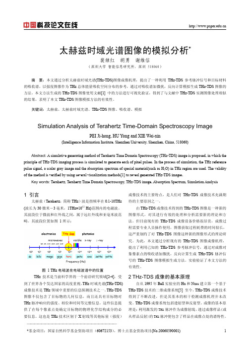
H(w)一般也称为样品在空间位置(x, y)处的吸收谱。 其它如色 图 2 透射型 THz 成像原理示意图 下面对图 2 成像过程作简单介绍: 由飞秒激光器发射的超短激光脉冲经过分光镜分为泵 浦光和探测光。泵浦光激发 THz 波发射器产生 THz 辐射, 经过聚焦后照射并透过样品上的某一点, 然后到达 THz 接收 器(一般为电光晶体) ,而探测光在通过光学延迟到达 THz 接收器的瞬间,记录检测到的 THz 光脉冲的电场强度。通过 控制并改变时延系统的时间参数,也就改变了探测光到达 THz 接收器的时间。当探测光到达时间变化时,就检测到了 随时间变化的 THz 脉冲电场强度。 为了便于对样品的 THz 特性进行分析,一般在对样品成 像的同时,还需记录在不放置样品时的 THz 脉冲,该脉冲信 号称为参考脉冲。 (a) (b) 散谱、折射率谱也可用类似方法计算得到。 图 3 给出了一个具体的 THz 参考脉冲,以及某物质的 THz 采样脉冲、频谱和吸收谱的图示。
该图像的数据量为 M×N×T×L 比特。THz-TDS 图像可以被 表示如下:
sTHz −TDS = f ( x, y, t )
素点 s(t)是一个由 T 维矢量表示的数字脉冲信号:
(1)
其中,0 ≤ x ≤ M, 0 ≤ y ≤ N, 0 ≤ t ≤ T。而空间位置(x, y)处的像
不同尺度的微分窗口下土壤有机质的一阶导数光谱响应特征分析_刘炜
第30卷第4期2011年8月红外与毫米波学报J.Infrared Millim.WavesVol.30,No.4August ,2011文章编号:1001-9014(2011)04-0316-06收稿日期:2010-05-30,修回日期:2010-10-17Received date :2010-05-30,revised date :2010-10-17基金项目:国家“973”计划项目(2007CB407203);国家自然科学基金项目(30872073);“十一五”国家科技支撑计划重大项目(2006BAD09B0603)作者简介:刘炜(1978-),男,陕西咸阳人,博士研究生,主要从事遥感与GIS 应用研究,E-mail :york5588@nwsuaf.edu.cn.*通讯作者:E-mail :chqr@nwsuaf.edu.cn.不同尺度的微分窗口下土壤有机质的一阶导数光谱响应特征分析刘炜1,常庆瑞1*,郭曼1,邢东兴1,2,员永生1(1.西北农林科技大学资源环境学院,陕西杨凌712100;2.咸阳师范学院资源环境系,陕西咸阳712000)摘要:使用高光谱仪ASD Field Spec 在波长范围400 1000nm 内采集有机质含量不同的土壤反射光谱数据并作对数变换处理;之后在不同尺度的微分窗口下求取其一阶导数(一阶导数光谱)并进行小波阈值去噪;从一阶导数光谱中提取特征参数表征有机质含量变化.结果表明,微分窗口尺度w =1 5时,土壤一阶导数光谱中含有大量噪声,对一阶导数光谱曲线形态和有机质吸收特征的识别造成严重干扰;微分窗口尺度w =6 15时,土壤一阶导数光谱中的噪声得到一定程度的去除,但仍无法准确判别有机质的吸收特征;微分窗口尺度w =16 30时,土壤一阶导数光谱中的噪声被有效去除,其中当w =19时,从一阶导数光谱中提取的特征参数MD 19s 与土壤有机质含量的相关系数为-0.803.MD 19s 能够较为准确地指示有机质含量变化,而且运算简单,易于实现,为在精准农业中采用可见/近红外反射光谱分析技术快速检测土壤有机质提供了新的途径.关键词:可见/近红外光谱;土壤有机质;一阶导数光谱;小波去噪;特征增强;特征提取中图分类号:S15文献标识码:AAnalysis on derivative spectrum feature for SOMunder different scales of differential windowLIU Wei 1,CHANG Qing-Rui 1*,GUO Man 1,XING Dong-Xing 1,2,YUAN Yong-Sheng 1(1.College of Resources and Environment ,Northwest A&F University ,Yangling 712100,China ;2.Department of Resources Environment ,Xian yang Normal College ,Xianyang 712000,China )Abstract :The hyper-spectral reflectance of soil was measured by a ASD FieldSpec within 400 1000nm ,then treated withlogarithmic transformation.First derivative of soil spectra with different scales of differential window were acquired and de-noised by the threshold denoising method based on wavelet transform.From the first derivative of soil spectra ,feature pa-rameters used as indicators for soil organic matter content were extracted.Results show that :(1)When the number of the scale of differential window was set as W =1 5,it is difficult to identify the spectrum contour and response feature in first derivative of soil spectra because of much noise.(2)When W =6 15,noise in first derivative of soil spectra is partly removed ,and spectrum contour is identified roughly.However spectral response feature resulted from different organic con-tent levels can not be identified clearly.(3)When W =16 30,noise in first derivative of soil spectrua is removed effec-tively.The coefficient of correlation between organic matter content and feature parameter MD 19s is 0.803.MD 19s can be used as one of the best indicators for soil organic matter content.Key words :VIS /NIR spectrum ;soil organic matter (SOM );first derivative of spectrum ;wavelet denoising ;feature enhancement ;feature extraction PACS :42.72.Ai引言传统的土壤有机质(Soil Organic Matter ,SOM )化学测定方法,虽然测定精度较高,但耗时、费力、成本高,而且还存在着有害、污染、测点数量和范围有限等问题.因而无法满足精准农业、变量施肥技术对4期刘炜等:不同尺度的微分窗口下土壤有机质的一阶导数光谱响应特征分析详细掌握土壤养分时空变异状况的需求.现代可见/近红外反射光谱分析技术,能够充分利用全谱段或多波长光谱数据进行定性或定量分析,并且具有速度快、成本低、效率高、测量方便、测试重现性好等特点,近年来,已经被越来越广泛地应用于食品工业、石油化工、农业、制药等多个领域[1-3].以往大量研究表明,可见/近红外光谱段400 1000nm是土壤有机质最主要的光谱响应区域,具有对有机质含量进行定量分析的潜力[4-6].一些研究[7-8]还表明对土壤高光谱数据进行导数变换,可以在一定程度上减弱土壤类型、样品粒度等因素的影响,有助于挖掘有机质的吸收特征.大量试验结果表明,当采用不同尺度的微分窗口对土壤高光谱数据进行导数变换时,所获取的土壤一阶导数光谱的形态会因光谱中高频噪声干扰程度的不同而产生较大差异.实际上,对高光谱数据进行导数变换,并不完全等同于从数学意义上对连续、可微函数进行求导运算,而是在一定尺度的微分窗口下,通过一阶差商实现对一阶求导的近似代替[9-11].当微分窗口取较小的尺度时,导数变换在提供精细的光谱形态变化信息的同时,也会放大光谱中的高频噪声,对光谱曲线上反射峰、吸收谷的识别、定位及相关计算造成严重干扰;当微分窗口取较大的尺度时,导数变换具有一定的平滑去噪功能(差分运算本质上也是一种加权数字平滑[1]),并且微分窗口尺度越大,曲线平滑效果越好.然而,在较大尺度的微分窗口下进行导数变换,也会对一阶导数光谱曲线上的极值点和拐点进行平滑,因而在降噪的过程中,也损失掉了光谱曲线上锐变尖峰成分可能携带的重要信息,导致光谱分析能力下降.因此,选取合适的微分窗口尺度,是从土壤一阶导数光谱中提取特征参数定量检测有机质含量的一个重要前提.试验在不同尺度的微分窗口下对土壤高光谱数据进行导数变换,并从一阶导数光谱中提取特征参数表征有机质含量变化,之后,分析微分窗口尺度变化对特征参数的影响.试验旨为在精准农业中采用可见/近红外光谱反射光谱分析技术定量检测土壤有机质,以及提高高光谱参数准确性和实用性方面提供依据.1材料与方法1.1样品采集与制备土壤样品采自陕西省眉县,采样区土壤为褐土,质地为壤质粘土,土层深厚.试验依据土壤剖面发生层次,分层采集土壤样品,采样深度为0 60cm.为了从光谱数据中消除或降低土壤水分、土壤粒度等因素的对土壤有机质吸收特征的影响,试验将土壤样品置于实验室内自然风干,之后用木棍滚压,并去除沙砾石块及植物残体,接下来研磨、过筛(100目尼龙筛).试验获取土壤样品36个,每个土壤样品分成两份,一份采用重铬酸钾法测定土壤有机质含量,另一份用来测量光谱数据.36个样本中,有机质含量的最大值为43.91g*kg-1,最小值为2.11g* kg-1,平均值为13.72g*kg-1.1.2光谱测量使用高光谱仪ASD Field Spec在波长范围350 1050nm内,连续测量经预处理后的土壤样品的反射光谱数据,光谱采样间隔1.4nm,重采样间隔1nm.测量光谱前将土壤样品放置在直径16cm,深度3cm 的盛样皿上,调整盛样皿使其处于水平位置,平整土样表面使样品厚度均匀.暗室内测试光源为能够提供平行光的1000W的镁光灯,距土壤表层中心70cm,光源照射方向与垂直方向的夹角为15ʎ.经多次实验后光纤探头的视场角选定为7.5ʎ,置于离土样表面40cm的垂直上方接收光谱数据.测试前以白板定标,每个土壤样品采集10条光谱数据,然后将其算术平均值作为该土壤样品的实际光谱反射数据.1.3数据处理可见/近红外光谱段400 1000nm是土壤有机质最主要的光谱响应区域.然而,该波长范围内土壤光谱反射率水平整体较低,有机质含量不同的各条光谱曲线之间距离较近,没有显著的峰谷特征,不利于特征参数提取[1].为此,试验在波长范围400 1000nm内对土壤原始光谱进行对数变换和导数变换,以增强有机质含量变化引起的光谱响应差异.对数变换采用的计算公式为[10-12]A(λ)=Ln[1/R(λ)],(1)式中:λ代表波长位置,取值区间为400 1000nm;R(λ)代表波长位置λnm处的土壤原始光谱反射率;A(λ)是经对数变换处理后的光谱值.导数变换采用的计算公式为[1]D(λ)=[A(λ)–A(λ+w)]/w,(2)式中w代表微分窗口尺度;D(λ)代表波长位置λnm处土壤光谱反射率的一阶导数;λ的取值区间为400 1000nm.2结果与分析2.1对数变换对土壤有机质一阶导数光谱响应特713红外与毫米波学报30卷征的影响图1(a )显示了波长范围400 1000nm 内,有机质含量不同(25.67,9.37,7.31,4.20g /kg )的土壤反射光谱曲线;图1(b )是对它们进行对数变换处理后的结果.从图1(b )中可以看出,在沿着波长增加的方向上,经对数变换处理后的光谱值大致以线性趋势从2.70下降至0.80,变动区间较原始光谱有所增加;对于不同的有机质含量水平,光谱曲线整体上随有机质含量水平的提高而提高,表现出正相关性;各条光谱曲线之间的距离较图1(a )中的也有所加大.整体而言,400 1000nm 内,土壤有机质含量的变化可以从图1(b )光谱曲线的分异表现中得到一定程度的反映,但有机质含量不同的各条光谱曲线仍大致以线性趋势变化,并且没有反映样品信息突出的反射峰、吸收谷.图1对数变换对土壤光谱反射率的影响Fig.1Effect of logarithmic transformation on soil spec-tra under different organic matter content levels2.2不同尺度的微分窗口对土壤有机质一阶导数光谱响应特征的影响在不同尺度的微分窗口下(w =1,2,…,30),求取对数变换后的土壤光谱的一阶导数(一阶导数光谱),结果如图2所示;图3则显示了一阶导数光谱与有机质含量之间的相关系数.结合图2与图3可以看出,随着微分窗口尺度的逐渐增大,导数变换的平滑效果越来越明显.w =1 5时,微分窗口的尺度较小,导数变换的平滑作用较为有限,一阶导数光谱曲线上仍保留有大量噪声,致使曲线轮廓以及因有机质含量变化引起的响应特征受到遮蔽干扰,难以识别,敏感波段无法提取,光谱质量较差;并且在对应的微分窗口尺度下,波长范围400 1000nm 内,相关系数曲线振荡强烈,频率高、幅度大,表现很不稳定.w =6 15时,随着微分窗口尺度的逐渐增大,导数变换的平滑作用有所提升,光谱噪声得到了一定程度的去除,土壤一阶导数光谱曲线的大致轮廓能够被识别出来;但波长范围400 1000nm 内,因有机质含量变化引起的光谱响应特征仍受到较强噪声的干扰,无法准确判别;对应微分窗口尺度下的相关系数曲线,仍然振荡频繁、起伏较大,不利于敏感波段提取.图2不同尺度的微分窗口对土壤一阶导数光谱响应特征的影响Fig.2First derivative of soil spectra under different soil matter organic content levels and different scales of differ-ential window8134期刘炜等:不同尺度的微分窗口下土壤有机质的一阶导数光谱响应特征分析图3不同尺度的微分窗口对土壤一阶导数光谱与有机质含量相关系数的影响Fig.3Correlation coefficients between organic matter contents and first derivative of soil spectra under differ-ent scales of differential windoww =16 30时,随着微分窗口尺度的不断增大,导数变换对光谱曲线的平滑作用进一步加强,土壤一阶导数光谱中的噪声得到有效去除,曲线轮廓更加清晰.从图2(c )中还可以发现,波长范围450 600nm 内,有机质含量不同的各条光谱曲线均存在一个“凸”状的特征峰;其中在“凸”状特征峰的核心区域,波长范围500 570nm 内,一阶导数光谱值维持在一个较高的平台上小幅振荡;对于不同的有机质含量水平,该波长范围内的光谱值随有机质含量的增加整体呈下降趋势,相对于其它波长位置,该波长范围内的光谱值表现出了较为一致、显著的响应特征.从图3(c )中还可以看出,波长范围500 570nm 内相关系数值小幅波动,表现较为稳定.鉴于w =16 30时,波长范围500 570nm 内的土壤一阶导数光谱值相互之间比较接近,而且波动程度不大;对有机质含量变化,整体上也表现出了较为一致、显著的响应特征,试验考虑以该波长范围内光谱值的平均值作为特征参数表征有机质含量变化.采用的计算公式为MD w s=171·∑570λ=500D w s(λ),(3)式中,λ代表波长位置;w 代表微分窗口尺度,w =1,2,…,30;D w s (λ)代表经对数变换处理后,微分窗口尺度为w ,波长位置λnm 处的土壤一阶导数光谱值;MD w s 则是波长范围500 570nm 内D ws (λ)的平均值.接下来,试验进一步计算了当微分窗口取不同的尺度时,MD w s 与土壤有机质含量之间的相关系数,结果如图4(a )所示.从图中可以看出,随着微分窗口尺度的逐渐扩展,相关系数曲线先下降、后上升,大体上呈开口向上的“凹”状波形;其中,在“凹”状波形的前段,当微分窗口取较小的尺度时,相关系数曲线有一定的起伏波动;当微分窗口尺度w =16 20时,相关系数值处于“凹”状波形的底部区域,基本保持在-0.800 -0.805之间,变化趋势十分稳定;其中,w =19时,相关系数取得负的最小值-0.803.显然,在所有的微分窗口尺度中,当w =19时得到的MD 19s 更适合用作特征参数指示有机质含量变化.2.3不同尺度的微分窗口对小波去噪后一阶导数光谱响应特征的影响为了进一步分析微分窗口尺度变化对土壤有机质一阶导数光谱响应特征的影响,试验对各个微分窗口尺度下的土壤一阶导数光谱,进行了小波阈值去噪处理(以“sym8”作为小波母函数,分解尺度J =3,选择“Heursure ”阈值选取规则和“sln ”阈值调整方法[13,14]),结果如图5所示.从中可以看出,经小波阈值去噪处理后,各个微分窗口尺度下的土壤一阶导数光谱的曲线轮廓,都变得十分清晰、光滑;波长范围450 600nm 内的“凸”状特征峰在不同的有机质含量水平下的分异表现也较为明显.同样,为了表征土壤有机质含量变化,试验在不同尺度的微分窗口下,求取波长范围500 570nm 内经小波去噪后的一阶导数光谱值的平均值MD wd 作为特征参数,采用的计算公式为MD w d=171·∑570λ=500D w d(λ),(4)式中λ代表波长位置;w 代表微分窗口尺度,w =1,913红外与毫米波学报30卷图4不同尺度的微分窗口对特征参数的相关系数的影响Fig.4Correlation coefficients between organic mat-ter contents and feature parameters under differentscales of differential window2,…,30;D wd(λ)代表经对数变换及小波阈值去噪处理后,微分窗口尺度为w的土壤一阶导数光谱值.MD wd 则是波长范围500 570nm内D wd(λ)的平均值.试验计算了MD wd与土壤有机质含量之间的相关系数,结果如图4(b)所示.从图中可以看出,当微分窗口尺度逐步扩展时,相关系数曲线呈开口向上、十分光滑的“凹”状波形,其整体变化趋势与图4(a)中相关系数曲线的整体变化趋势大体一致;但波动程度明显降低,曲线形态十分光滑;相对于图4(a),图(4)b中相关系数曲线的整体变动区间有所收窄,在-0.797 -0.753之间;当微分窗口尺度w =15 21时,相关系数值处于“凹”状波形的底部区域;其中,当w=20时,相关系数取得了负的最小值-0.797.对比MD19s 和MD20d,可以看出二者的微分窗口尺度值相差不大,对应的相关系数值也较为接近,但MD19s的表现更好一些;同时,其相关计算较MD20d也更容易实现、易于掌握、推广.故试验认为MD19s更适合用作特征参数指示有机质含量变化.3讨论可见/近红外光谱段400 1000nm是土壤有机图5不同尺度的微分窗口对去噪后的土壤一阶导数光谱响应特征的影响Fig.5Denoised first derivative of soil spectrum under different soil matter organic content levels and different scales of differenti-al window质最主要的光谱响应区域.然而,在该波长范围内,土壤光谱反射率水平整体较低,有机质含量不同的各条光谱曲线之间距离较近,没有显著的峰谷特征,不利于特征参数提取[1].为此,试验对土壤原始光谱进行对数变换,以增强有机质含量变化引起的光谱响应差异.除对数函数外,还可以选取其它具有较强放大增益的函数,如正切函数、指数函数等作为变换函数对有机质的响应特征进行增强处理.此外,还可以考虑针对能够反映有机质吸收特性的敏感波段,给变换函数的自变量赋以一定的偏移量,以尽可能地将敏感波段置于具有最佳放大增益效果的对应的自变量的取值区间,进一步提升某些特定敏感波段在解释有机质含量变化中的作用.在可见/近红外反射光谱分析技术中,利用导数变换可以获取精细的光谱形态变化信息,并能够增强局部位置(如极值点、拐点等)光谱反射率对目标物质含量变化的响应差异.对于土壤高光谱数据,除一阶导数变换外,还可以在选取具有合适尺度的微分窗口的前提下,考虑采用二阶或三阶等更高阶次导数变换,以进一步挖掘因有机质吸收引起的峰谷特征;之后,根据反射峰(吸收谷)的形态,选择合适的吸收特征描述方法,以提取稳定性更强,敏感程度也好的特征参数表征有机质含量变化.4结论试验对土壤原始光谱进行了对数变换,导数变0234期刘炜等:不同尺度的微分窗口下土壤有机质的一阶导数光谱响应特征分析换以及小波阈值去噪处理;之后,在不同尺度的微分窗口下分析土壤一阶导数光谱对有机质含量变化的响应特征,并提取特征参数MD ws 和MD wd.试验得到的结论如下:(1)微分窗口尺度w=1 5时,土壤一阶导数光谱中含有大量噪声,致使光谱曲线的形态和有机质的吸收特征难以识别,敏感波段无法提取,光谱质量较差.(2)微分窗口尺度w=6 15时,土壤一阶导数光谱中的噪声得到了一定程度的去除,光谱曲线的大致轮廓能够被识别出来,但因有机质含量变化引起的光谱响应差异仍无法得到准确判别.(3)微分窗口尺度w=16 30时,土壤一阶导数光谱中的噪声得到了有效地去除;波长范围450 600nm内呈现出“凸”状的特征峰;其中,在“凸”状特征峰的核心区域,波长范围500 570nm内,一阶导数光谱值对有机质含量变化整体表现了出较为一致、显著的响应特征.(4)特征参数MD19s与土壤有机质含量的相关系数为-0.803,相对于MD20d ,MD19s可以更好地用来指示有机质含量变化.波长范围400 1000nm内,土壤有机质吸收引起的光谱曲线的变化比较微弱,一般均先要求对土壤原始光谱进行某种变换,以增强光谱响应差异,之后提取特征参数检测有机质.在光谱特征增强的数学变换方法中,对数变换,指数函数变换、导数变换等都应用较多.可以针对光谱形态和有机质的吸收特性,对各种增强方法进行更加细致地调整、改进,或者加以综合运用,并选取恰当的吸收特征描述方法[1],以提取稳定性更强、敏感程度更好的特征参数,为采用可见/近红外反射光谱分析技术快速检测土壤有机质,提供更实用、有效的途径,这将是下一步研究工作重点.REFERENCES[1]LI Min-Zan,HAN Dong-Hai,WANG Xiu.Spectral analysis technology and its application[M].Beijing:Science Press (李民赞,韩东海,王秀.光谱分析技术及其应用.北京:科学出版社),2006:115-279.[2]HE Yong,SONG Hai-Yan,Pereira A G,et al.Measure-ment and analysis of soil nitrogen and organic matter content using near-infrared spectroscopy techniques[J].Journal of Zhejiang University SCIENCE,2005,6B(11):1081-1086.[3]BAO Yi-Dan,HE Yong,FANG Hui,et al.Spectral char-acterization and N content prediction of soil with different particle size and moisture content[J].Spectroscopy and Spectral Analysis(鲍一丹,何勇,方惠,等.土壤的光谱特征及氮含量的预测研究.光谱学与光谱分析),2007,27(1):62-65.[4]HE Ting,WANG Jing,LIN Zong-Jian,et al.Spectral fea-tures of soil organic matter[J].Geo-spatial Information Sci-ence,2009,12(1):33-40.[5]LIU Huan-Jun,ZHANG Bai,LIU Dian-Wei,et al.Study on quantitatively remote sensing typical soils in Songnen plain,northeast China[J].Journal of Remote Sensing(刘焕军,张柏,刘殿伟,等.松嫩平原典型土壤高光谱定量遥感研究.遥感学报),2008,12(4):647-654.[6]SHA Jin-Ming,CHEN Peng-Cheng,CHEN Song-Lin.Characteristics analysis of soil spectrum response resulted from organic material[J].Research of Soil and Water Con-servation(沙晋明,陈鹏程,陈松林.土壤有机质光谱响应特性研究.水土保持研究),2003,10(2):21-24.[7]Ben-Dor E.The reflectance spectra of organic matter in the visible near-infrared and short wave infrared region(400 2500nm)duing a controlled decompsition process[J].Ro-mote Sensing of Enviroment,1997,61:1-15.[8]SONG Hai-Yan,HE Yong.Determination of the phosphor-us,kalium contents and pH values in soils using near-infra-red spectroscopy[J].Journal of Shanxi Agricultural Univer-sity:Netural Science Edition(宋海燕,何勇.近红外光谱法分析土壤中磷、钾含量及pH值的研究.山西农业大学学报:自然科学版),2008,28(3):275-278.[9]WANG Ji-Hua,ZHAO Chun-Jiang,HUANG Wen-Jiang.Base and application of quantitative remote sensing technique in agriculture[M].Beijing:Science Press(王纪华,赵春江,黄文江.农业定量遥感基础与应用.北京:科学出版社),2008:156-159.[10]GONG Cai-Lan,YIN Qiu,KUANG Ding-Bo.Correlations between water quality indexes and reflectance spectra ofHuangpujiang river[J].Journal of Remote Sensing(巩彩兰,尹球,匡定波.黄浦江水质指标与反射光谱特征的关系分析.遥感学报),2006,10(6):910-916.[11]LI Xin-Zhen,CHE Gang-Ming,FENG Jian-Hu,et al.Computational methods[M].Xi’an:Northwestern Poly-technical University Press(李信真,车刚明,封建湖,等.计算方法.西安:西北工业大学出版社),2000:172-175.[12]WAN Yu-Qing,TAN Ke-Long,ZHOU Ri-Ping.Hyper-spectral remote sensing and its application[M].Beijing:Science Press(万余庆,谭克龙,周日平.高光谱遥感应用研究.北京:科学出版社),2006:22-189.[13]XU Wei-Dong,YIN Qiu,KUANG Ding-bo.Decision tree classification of hyperspectral image based on discretewavelet transform[J].Journal of Remote Sensing(许卫东,尹球,匡定波.小波变换在高光谱决策树分类中的应用研究.遥感学报),2006,10(2):204-210.[14]JIANG Qing-Song,WANG Jian-Yu.Study on signal-to-noise ratio estimtion and compression method of operationalmodular imaging spectrometer multi-spectral images[J].Acta Optica Sinica(蒋青松,王建宇.实用型模块化成像光谱仪多光谱图像的信噪比估算及压缩方法研究.光学学报),2003,23(11):1335-1340.123。
【材料研究方法】光谱分析(英文)

Vibrational spectroscopy6.3.7 Absorbant intensity and IR spectroscopyt r a n s m i t t a n c e Fig. 6-18 IR spectrum. s (strong )、m (medium )、w(weak )、vw (very weak )a b s o r b a n c eVibrational spectroscopy3334 cm -1–OH stretch. Normal range: 3350±150 cm -1. This is a verycharacteristic group frequency. All of the peaks due to the OH group are broad due to hydrogen bonding.Vibrational spectroscopy 3390 cm-1–NH2antisymmetric stretch.Normal range: 3300±100 cm-1. Muchweaker adsorption than the OH stretchin hexanol.Vibrational spectroscopy 3290cm-1–NH2symmetric stretch. 2°amines have only one NH stretch, and3°amines have none.Vibrational spectroscopy Spectral interpretation always starts at the high end, because there are the best group frequencies and they are the easiest to interpret. No peaks appear above 3000 cm-1, the cut-off for unsaturated C-H. the four peaks below 3000 cm-1 are saturated C-H stretching modes.Vibrational spectroscopy 3050 ±50 cm-1 corresponds to the aromatic orunsaturated C(sp2)-H stretch. Always above3000 cm-1. These bands are not assigned tospecific vibrational modes.Vibrational spectroscopy 3080cm-1=CH3080 cm1 2 antisymmetric stretch. An absorption above 3000 cm-1 indicates the presence of an unsaturation (double or triple bond or an aromatic ring).Vibrational spectroscopy 2247 cm-1 C≡N stretch. Normal range:2250±10 cm-1 , lowered 10-20 cm-1when conjugated. Compare to the C ≡Cstretch in 1-heptyne (3000 cm-1).Vibrational spectroscopy 1742 cm-1, -C=O stretch. In small ring esters, this vibration is shifted to higher frequency by coupling to the stretch ofthe adjacent of O-C and C-C bonds. The amount of coupling depends on the O-C(O)-C angle. As with other carbonyl groups, conjugation lowers the frequency.Vibrational spectroscopy 1642 cm-1, C=C stretch. Normalrange:164020cm-1for cis andrange: 1640±20 cm for cis andvinyl, 1670±10 cm-1for trans, tri andtetra substituted. Trans-2-hexene(overlay menu) has only a very weakabsorption, because there is verylittle dipole change when an internaldouble bond stretches (it is nearlysymmetric).Vibrational spectroscopyThe broad peak at approximately 1460 cm-1is actually two overlapping peaks. At1640±10 cm-1, the antisymmetric bend ofthe CH3group absorbs. This is a degenerage bend (one shown).Vibrational spectroscopy At 1375 ±10cm-1, the CH3 symmetric bend (also called the“umbrella” bend) absorbs. This peak is very useful becauseit is isolated from the other peaks. Compare the spectrum ofcyclohexane. The most prominent difference between thetwo spectra is the absence of a CH3 symmetric bend in thecyclohexane spectrum./cm-11715 1800 1828 1928。
拉曼光谱测量钙钛矿电声耦合强度
拉曼光谱测量钙钛矿电声耦合强度1.拉曼光谱是一种用于分析晶体材料结构和性质的强大技术。
Raman spectroscopy is a powerful technique for analyzing the structure and properties of crystalline materials.2.钙钛矿是一类具有重要电声耦合特性的材料。
Perovskite is a type of material with important electroacoustic coupling properties.3.通过拉曼光谱,可以了解钙钛矿中电声耦合的强度和机制。
Raman spectroscopy can be used to understand the strength and mechanism of electroacoustic coupling in perovskite.4.钙钛矿的电声耦合特性对于光伏和光电器件的性能至关重要。
The electroacoustic coupling properties of perovskite are crucial for the performance of photovoltaic and optoelectronic devices.5.拉曼光谱可以提供关于晶体结构、相变和电子结构的丰富信息。
Raman spectroscopy can provide rich information about crystal structure, phase transitions, and electronic structure.6.钙钛矿材料的电声耦合性质直接影响着其光电器件的效率和稳定性。
The electroacoustic coupling properties of perovskite materials directly affect the efficiency and stability oftheir optoelectronic devices.7.拉曼光谱测量可以帮助科学家们深入了解钙钛矿材料的微观特性。
基于深度学习的Fano_共振超材料设计

第 16 卷 第 4 期中国光学(中英文)Vol. 16 No. 4 2023年7月Chinese Optics Jul. 2023文章编号 2097-1842(2023)04-0816-08基于深度学习的Fano共振超材料设计杨知虎,傅佳慧,张玉萍,张会云*(山东科技大学 电子信息工程学院 青岛市太赫兹技术重点实验室, 山东 青岛, 266590)摘要:本文提出了一种基于深度学习的超材料Fano共振设计方法,能够获得高Q共振的线宽、振幅和光谱位置特性。
利用深度神经网络建立结构参数和透射谱曲线之间的映射,正向网络实现对透射谱的预测,逆向网络实现对高Q共振按需设计,设计过程中实现了低均方误差(MSE),训练集的均方误差为 0.007。
与传统方法需要耗时的逐个数值模拟相比,深度学习设计方法大大简化了设计过程,实现了高效、快速的设计目标。
对Fano共振的设计也可推广应用到其它类型的超材料的自动逆向设计,显著提高了更复杂的超材料设计的可行性。
关 键 词:超材料;神经网络;Fano共振;逆向设计;深度学习中图分类号:O436.3 文献标志码:A doi:10.37188/CO.2022-0208Fano resonances design of metamaterials based on deep learningYANG Zhi-hu,FU Jia-hui,ZHANG Yu-ping,ZHANG Hui-yun*(Qingdao Key Laboratory of Terahertz Technology, College of Electronic and Information Engineering, Shandong University of Science and Technology, Qingdao 266590, China)* Corresponding author,E-mail: sdust_thz@Abstract: In this paper, a metamaterial Fano resonance design method based on deep learning is proposed to obtain high-quality factor (high-Q) resonances with desired characteristics, such as linewidth, amplitude, and spectral position.The deep neural network is used to establish the mapping between the structural parameters and the transmission spectrum curve. In the design, the forward network is used to predict the transmission spectrum, and the inverse network is used to achieve the on-demand design of high Q resonance. The low mean square error ( MSE ) is achieved in the design process, and the mean square error of the training set is 0.007. The results indicate that compared with the traditional design process, using deep learning to guide the design can achieve faster, more accurate, and more convenient purposes. The design of Fano resonance can also be extended to the automatic inverse design of other types of metamaterials, significantly improving the feasibility of more complex metamaterial designs.Key words: metamaterials;neural networks;Fano resonance;reverse engineering;deep learning收稿日期:2022-10-10;修订日期:2022-11-11基金项目:国家自然科学基金(No. 61875106,No. 62105187);山东省自然科学基金(No. ZR2021QF010)Supported by National Natural Science Foundation of China (No. 61875106, No. 62105187); Natural ScienceFoundation of Shandong Province (No. ZR2021QF010)1 引 言1961年,Fano U[1]在其原子自电离态的量子力学机理的研究中,发现了Fano共振现象。
211050369_分散固相萃取-超高效液相色谱-串联质谱法测定海龙中11_种磺胺类抗菌药物残留
分析测试新成果 (16 ~ 22)分散固相萃取-超高效液相色谱-串联质谱法测定海龙中11种磺胺类抗菌药物残留王小乔1 ,李 坚1 ,许晓辉1 ,李剑勇2 ,吴福祥1 ,张虹艳1 ,潘秀丽1 ,李 赟1(1. 兰州市食品药品检验检测研究院/食品中农药兽药残留监控国家市场监管重点实验室,甘肃 兰州 730050;2. 中国农业科学院 兰州畜牧与兽药研究所,甘肃 兰州 730050)摘要:采用超高效液相色谱串联三重四极杆质谱(UPLC-MS/MS )技术,建立了测定海龙中11种磺胺类抗菌药物残留量的分析方法. 样品经2%甲酸-乙腈超声提取,增强型脂质去除分散固相萃取净化管(EMR-Lipid dSPE )净化,采用Waters ACQUITY BEH C 18色谱柱(1.7 µm ,2.1 mm×100 mm )分离,电喷雾离子源电离,正离子多反应监测模式(MRM )检测,以含2 mmol/L 乙酸铵-0.1%甲酸的水溶液和含0.1%甲酸的乙腈溶液为流动相进行梯度洗脱,外标法定量. 11种磺胺类抗菌药物在0~30 ng/mL 的质量浓度范围内线性关系良好,相关系数(R 2)均不低于0.995 9,检出限(LOD )与定量限(LOQ )分别在0.11~1.30 µg/kg 和0.37~4.40 µg/kg 之间,11种磺胺类抗菌药物在质量浓度为20.0、50.0、100.0 µg/kg 时的三个加标水平的平均回收率为62.5%~118.1%,相对标准偏差为2.1%~9.2%. 方法前处理简便、准确性好,可用于海龙中11种磺胺类抗菌药物残留的快速筛查.关键词:海龙;超高效液相色谱-三重四极杆质谱联用法;磺胺类药物;分散固相萃取;残留量中图分类号:O657. 63 文献标志码:B 文章编号:1006-3757(2023)01-0016-07DOI :10.16495/j.1006-3757.2023.01.003Determination of 11 Sulfonamide Antibacterial Drug Residues in Syngnathus by Ultra-Performance Liquid Chromatography-Mass Spectrometry Combined with Dispersed Solid Phase ExtractionWANG Xiaoqiao 1, LI Jian 1, XU Xiaohui 1, LI Jianyong 2, WU Fuxiang 1, ZHANG Hongyan 1,PAN Xiuli 1, LI Yun1(1. Lanzhou Institute for Food and Drug Control/Key Laboratory of Pesticides and Veterinary Drugs Monitoringfor State Market Regulation , Lanzhou 730050, China ;2. Lanzhou Institute of Husbandry and Pharmaceutical Sciences of CAAS , Lanzhou 730050, China )Abstract :An analytical method for the determination of 11 sulfonamide antibacterial drug residues in Syngnathus by ultra-performance liquid chromatography-mass spectrometry (UPLC-MS/MS) has been established. The samples were extracted by ultrasonication with 2% formic acid-acetonitrile, purified by an enhanced matrix removal lipid-dispersed solid phase extraction (EMR-Lipid dSPE), and separated on a Waters ACQUITY BEH C 18 column (1.7 µm, 2.1 mm×100mm). The analytes were detected by mass spectrometry using the positive electrospray ionization mode under multiple reaction monitoring mode (MRM), with 2 mmol/L ammonium acetate-0.1% formic acid in aqueous solution and 0.1%收稿日期:2022−10−19; 修订日期:2023−01−08.基金项目:甘肃省市场监督管理局科技计划资助项目(SSCJG-SP-A202204)作者简介:王小乔(1973−),女,本科,研究方向:食品药品检验检测与研究,E-mail :通信作者:李坚(1969−),男,本科,主管药师,研究方向:食品药品检验检测与研究,E-mail :.第 29 卷第 1 期分析测试技术与仪器Volume 29 Number 12023年3月ANALYSIS AND TESTING TECHNOLOGY AND INSTRUMENTS Mar. 2023formic acid in acetonitrile as mobile phases by a gradient elution program, and quantified by the external standard method. The results showed that the 11 antibacterial sulfonamides had good linearity in the range of 0~30 ng/mL, the correlation coefficient (R2) were all greater than 0.9959, the limit of detection (LOD) and quantitation (LOQ) were in the range of 0.11~1.30 µg/kg and 0.37~4.40 µg/kg, respectively. At three spiked levels of 20.0, 50.0 and 100.0 µg/kg, the spiked average recoveries of the analytes were in the range of 62.5%~118.1%, and the relative standard deviation was 2.1%~9.2%. The method is accurate, straightforward, and is suitable for the rapid screening of 11 sulfonamide antibacterial drug residues in Syngnathus.Key words:Syngnathus;UPLC-MS/MS;sulfonamides;solid phase extraction;residues海龙是一种药用价值很高的动物源性中药材,也是一种水产品,其为刁海龙Solenognathus hardwickii(Gray)、拟海龙Syngnathoidesbiaculeatus (Bloch)或尖海龙Syngnathus acus Linnaeus的干燥体[1-4],主要成分是甾体类、脂肪酸、蛋白质、氨基酸、微量元素等,具有温肾壮阳、散结消肿等功效,广泛应用于临床治疗中[5]. 因野生海龙资源稀缺,市场所见海龙主要来源于人工养殖. 在海龙养殖过程中,养殖户为了避免其受细菌感染而造成经济损失,常使用磺胺类药物进行预防治疗. 但有些不良养殖户违规超量使用磺胺类药物,导致药物残留在海龙体内,人类通过食用海龙进而转移到人体内[6-8]. 人类若食用磺胺类药物残留量较高的海龙,易产生药物蓄积,导致肾毒性与过敏反应,甚至会破坏胃肠道菌群平衡,引起白细胞减少等[9-10]. 当前,有关海龙中磺胺类抗菌药物残留量的常规监测未见文献报道,因此,从安全角度出发,很有必要建立简便、可靠的方法以满足海龙中磺胺类药物残留检测的需求.目前,测定动物源性食品中磺胺类药物应用最广泛的是超高效液相色谱-串联质谱法,其具有背景干扰少、灵敏度高、特异性强、选择性强等特点,适合复杂基质中微量成分的检测. 前处理方法应用最广泛的是分散固相萃取和固相萃取柱[11-14]. 传统的分散固相萃取难以去除动物源性食品中大部分脂质干扰物,固相萃取柱因需要活化、淋洗、洗脱和浓缩等,试验过程繁琐. 而增强型脂质去除分散固相萃取(enhanced matrix removal lipid-dispersed solid phase extraction,EMR-Lipid dSPE)可选择性去除样品中的主要脂类且不影响目标分析物的提取效率,相比传统的分散固相萃取和固相萃取柱,EMR-Lipid dSPE具有操作简单、杂质净化高效的优势.为了监测与评判海龙中磺胺类药物残留的暴露水平与风险,本研究采用2%甲酸-乙腈提取干燥样品中的目标待测物,使用EMR-Lipid dSPE净化技术去除脂类等非极性杂质,建立了一种基于超高效液相色谱质谱联用法同时测定海龙中11种磺胺类抗菌药物残留量的分析方法. 该方法快速简单、重复性好、定量准确,适用于海龙中磺胺类药物残留的风险监测.1 试验部分1.1 仪器与试剂Agilent 1290 Infinity II-6460C超高效液相色谱串联三重四极杆质谱联用仪(配置离子源为Agilent Jet Stream电喷雾离子源)、EMR-Lipid dSPE净化管(美国安捷伦科技有限公司);MS105DU型电子天平(瑞士梅特勒托利多有限公司);VXR涡旋混合器(德国艾卡仪器设备有限公司);H1850离心机(湖南湘仪实验室仪器开发有限公司);SB-800DT超声波清洗机(宁波新芝生物科技股份有限公司).乙腈(色谱纯,德国默克公司);乙酸铵、甲酸(色谱纯,日本东京化成工业株式会社);蒸馏水(广州屈臣氏食品饮料有限公司);其余试剂均为分析纯. 对照品:磺胺甲基嘧啶(批号:G982705,纯度:99.1%)、磺胺甲噁唑(批号:G150000,纯度:99.5%)、磺胺氯哒嗪(批号:G119228,纯度:99.1%)、磺胺邻二甲氧嘧啶(批号:G151421,纯度:99.1%)、磺胺噻唑(批号:G980077,纯度:99.2%)、磺胺间二甲氧嘧啶(批号:G122608,纯度:99.5%)、磺胺甲二唑(批号:G974370,纯度:99.3%)、磺胺甲氧哒嗪(批号:G150001,纯度:99.7%)均来源于德国Dr.Ehrenstorfer GmbH公司;磺胺嘧啶(批号:100026-201404,纯度:99.7%)、磺胺二甲嘧啶(批号:100411-200501,纯度:100%)来源于中国食品药品检定研究院;磺胺间甲氧嘧啶(批号:97864,纯度:99.1%)来源于曼哈格生物科技有限公司. 实际检测样品的信息如下:甘肃第 1 期王小乔,等:分散固相萃取-超高效液相色谱-串联质谱法测定海龙中11种磺胺类抗菌药物残留17中医药大学附属医院2批(批号:20141101);广西蓝正药业有限责任公司2批(批号:200901);甘肃陇脉药材有限公司1批(批号:190701).1.2 对照品溶液配制精密称取11种磺胺类药物对照品10.0 mg,分别置于10 mL棕色容量瓶中,加适量乙腈并超声使其溶解,取出放至室温,使用乙腈稀释至刻度,摇匀,得到质量浓度均为1 mg/mL的对照品储备溶液,于−18 ℃下保存备用. 分别准确吸取上述各对照品储备溶液0.025 mL,置于同一个25 mL的棕色容量瓶中,使用乙腈稀释至刻度,摇匀,得到质量浓度均为1 µg/mL的混合对照品中间溶液,于−18 ℃下保存备用. 再精密移取1.00 mL上述混合对照品中间溶液,置于10 mL棕色容量瓶,用乙腈稀释至刻度,摇匀,得到质量浓度均约为100 ng/mL的磺胺类药物混合对照品溶液,于4 ℃冷藏备用.1.3 供试品溶液配制取适量供试样品,粉碎,精密称取1 g,置于50 mL容量瓶中,加入2 mL水复原,静置20 min,精密加入10.00 mL 2%甲酸-乙腈,涡旋振荡2 min,超声处理20 min,再加入4 g硫酸钠和1 g氯化钠,涡旋振荡2 min,在3 900 r/min转速下离心15 min,精密移取上层清液2.00 mL置于EMR-Lipid dSPE 净化管,涡旋振荡1 min,在3 900 r/min转速下离心20 min,取上层清液,过0.22 µm有机滤膜,上机测定.1.4 色谱条件色谱柱:Waters ACQUITY BEH C18色谱柱(1.7µm,2.1 mm×100 mm). 流动相:A相为含2 mmol/L 乙酸铵和0.1%甲酸的水溶液,B相为含0.1%甲酸的乙腈溶液,梯度洗脱程序如下:0~1.0 min,15% B;1.0~2.0 min,30% B;2.0~3.0 min,40% B;3.0~4.5 min,90% B;4.5~6.5 min,90% B;6.5~7.0 min,15% B;7.0~8.0 min,15% B. 柱温:35 ℃;进样量:2 µL;流速:0.2 mL/min.1.5 质谱条件离子源:安捷伦喷射流电喷雾离子源(agilent jet stream electron spray ionization,AJS ESI);离子极性:正离子;采集模式:多反应监测模式(multiple reaction monitoring,MRM);气流温度:325 ℃;雾化气:N2;干燥气流速:6 L/min;雾化器压强:0.31 MPa;鞘气流速:10 L/min;鞘气温度:350 ℃;毛细管电压:4 000 V;各个磺胺类药物的质谱参数及保留时间如表1所列.2 结果与讨论2.1 前处理条件选择本试验检测的11种磺胺类药物在甲醇、乙腈中均能够很好的溶解,大多数被测目标化合物与乙腈极性接近,且乙腈能变性并沉淀蛋白,故选择乙腈作为海龙中磺胺类药物的提取溶剂. 由于磺胺类药物在酸性条件下容易发生质子化,酸化提取溶剂表 1 11种磺胺类药物的质谱参数及保留时间Table 1 Mass spectrum parameters and retention times of 11 sulfonamides序号名称保留时间/min母离子/(m/z)子离子/(m/z)碎裂电压/V碰撞能量/eV 1磺胺甲噁唑 4.665254.1156.0*/108.010010/25 2磺胺氯哒嗪 4.449285.0156.0*/108.010010/25 3磺胺间甲氧嘧啶 4.006281.1156.0*/108.010515/25 4磺胺甲基嘧啶 3.607265.1172.0/156.0*11012/15 5磺胺邻二甲氧嘧啶 4.585311.1156.0*/92.012015/30 6磺胺间二甲氧嘧啶 5.067311.0156.0*/108.013020/26 7磺胺二甲嘧啶 3.950279.1186.1*/156.112015/16 8磺胺嘧啶 2.902251.1156.0*/108.010010/22 9磺胺甲二唑 3.969271.0156.0*/108.09010/22 10磺胺噻唑 3.208256.0156.0*/108.010010/21 11磺胺甲氧哒嗪 4.287281.1156.0*/108.010515/25注:“*”为定量离子18分析测试技术与仪器第 29 卷有助于目标物的提取,本试验考察了在10 ng/mL 加标质量浓度下,乙腈、1%甲酸-乙腈、2%甲酸-乙腈、5%甲酸-乙腈的提取回收率和质谱响应. 结果发现,11种磺胺类药物在甲酸酸化乙腈中的质谱响应优于乙腈,当提取溶剂为2%甲酸-乙腈时,大部分磺胺类药物的质谱响应及提取回收率都优于其他甲酸酸化方案(如图1所示). 而EMR-Lipid dSPE 是一种新型分散固相萃取技术,常被用在QuEChERS 和蛋白质沉淀等净化流程中,可有效去除海龙中非极性的基质杂质,能够提高基质去除效率和分析重现性,与传统分散固相萃取相比,提高了净化效果.与固相萃取柱相比,净化流程简单快速,无繁琐的活化、上样、淋洗以及洗脱等步骤. 因此本试验最终采用2%甲酸-乙腈提取样品中目标待测物,EMR-Lipid dSPE 净化.2.2 色谱及质谱条件优化磺胺类药物含有相同的母体结构,在酸性条件下容易发生质子化,本试验选用了通用型超高效色谱柱Waters ACQUITY BEH C 18. 在正离子多反应监测采集模式下,流动相中加入适量甲酸能提高电喷雾源对目标检测物的离子化效率,加入适量乙酸铵能减少拖尾并改善峰形,因此选择在乙腈与水中加入不同浓度的甲酸、乙酸铵,考察峰形对称性、灵敏度与分离效果,寻找最佳流动相组合. 结果表明,在水相中加入2 mmol/L 乙酸铵和0.1%甲酸能显著改善峰形、提高灵敏度,在有机相中加入0.1%甲酸能提高离子化效果与重现性,稳定保留时间. 因此本试验采用含2 mmol/L 乙酸铵与0.1%甲酸的水溶液、含0.1%甲酸的乙腈作为流动相.分别将对照品溶液直接注入质谱仪,在正离子采集模式下,以全扫描(Scan )确定化合物准分子离子. 以选择离子扫描(Sim )确定碎裂电压,以子离子扫描(Product ion )确定丰度最高的2个子离子,分别作为定性离子与定量离子. 以多反应监测扫描(MRM )确定定性离子与定量离子的最佳碰撞能量,建立的仪器采集方法包含化合物名称、定性定量离子对、碰撞能量、碎裂电压以及驻留时间等.以多反应监测模式采集11种磺胺类抗菌药物的定性、定量离子对色谱图,其质量浓度为20ng/mL 的混合对照品溶液的提取离子流图如图2所示. 由图2可见,各个目标检测物监测通道互不干扰,所得采集峰形对称且响应良好.2.3 基质效应基质效应影响测定结果的准确性,因此,评价基质产生的基质效应十分有必要. 本试验通过考察同一浓度的空白样品基质溶液匹配混合对照品溶液,与2%甲酸-乙腈匹配混合对照品溶液质谱响应强度比值的百分比来评价基质效应(matrix effect ,ME ). ME 为(100±20)%,通常认为ME 弱. ME 大于120%或小于80%,分别为存在增强或抑制效应.如图3所示,磺胺间二甲氧嘧啶存在弱的增强效应,磺胺噻唑存在抑制效应,除此之外,其他目标检测物的基质效应较弱. 总体来说,基质效应不影响所有目标检测物的分析结果.2.4 方法学考察2.4.1 线性关系、检出限和定量限使用乙腈将混合对照品溶液依次稀释配制成质量浓度为0、1、2、5、10、20、30 ng/mL 的标准曲线磺胺间甲氧嘧啶磺胺甲噁唑回收率/%乙腈1% 甲酸乙腈2% 甲酸乙腈5% 甲酸乙腈140120100806040200磺胺氯哒嗪磺胺甲基嘧啶磺胺邻二甲氧嘧啶磺胺甲氧哒嗪磺胺间二甲氧嘧啶磺胺二甲嘧啶磺胺嘧啶磺胺甲二唑磺胺噻唑图1 不同提取溶剂的提取效率Fig. 1 Extraction efficiencies of different extraction solvents第 1 期王小乔,等:分散固相萃取-超高效液相色谱-串联质谱法测定海龙中11种磺胺类抗菌药物残留19溶液,外标法定量,以11种磺胺类药物的浓度(x )为横坐标,以定量离子的响应值(y )为纵坐标,绘制标准曲线. 取空白样品,逐级减少加入混合对照品溶液,按1.3项下方法处理样品,上机测定. 由提取的MRM 色谱图,以信噪比为3对应的质量浓度作为检出限(LOD ),以信噪比为10对应的质量浓度作为定量限(LOQ ),结果如表2所列. 由表2可见,11种目标检测物在0~30 ng/mL 的质量浓度范围内,线性关系良好,相关系数R 2不低于0.995 9,LOD 为0.11~1.30 µg/kg ,LOQ 为0.37~4.40 µg/kg.2.4.2 回收率与精密度选用海龙空白样品,分别添加20.0、50.0、100.0µg/kg 3个浓度水平的混合对照中间液,按照前处理方法处理后上机测定,每个浓度水平平行进行6次试验,每份待测样品溶液重复测定2次,计算回收率与精密度(RSD ),结果如表3所列. 由表3可见,11种目标待测物的平均回收率为62.5%~118.1%,RSD (n=6)为2.1%~9.2%,建立的分析方法完全能够满足实际样品的检测需求.2.5 样品测定采用本方法对5批海龙样品中11种磺胺类抗菌药物残留量进行测定,结果未检出目标检测物,如图4所示(其中1批阴性样品总离子流图),说明市售海龙中上述11种磺胺类抗菌药物残留在一定程度上处于低风险等级.3 结论本研究采用2%甲酸-乙腈作为提取溶剂,超声提取样品中目标待测物,EMR-Lipid dSPE 净化提取液,以正离子多反应监测模式检测,同时优化了液相色谱质谱检测条件,建立了一种超高效液相色谱质谱联用法同时测定海龙中11种磺胺类药物残留的分析方法,并进行了相关的方法学考察. 该方法具有线性关系良好、灵敏度高、准确度和精密度好的特点,且前处理简单、净化高效. 基质效应评价显示,虽然目标检测物存在不同程度的基质效应,但磺胺甲噁唑磺胺氯哒嗪磺胺间甲氧嘧啶磺胺甲基嘧啶磺胺邻二甲氧嘧啶磺胺甲氧哒嗪磺胺间二甲氧嘧啶磺胺二甲嘧啶磺胺嘧啶磺胺甲二唑磺胺噻唑2.0×10³C o u n t s1.8×1031.6×1031.4×1031.2×1031.0×1030.8×1030.6×1030.4×1030.2×10300.81.2 1.62.0 2.4 2.83.23.64.44.0Acquisition time/min4.85.2 5.66.0 6.4 6.87.27.68.0图2 11种磺胺类药物对照品提取离子流图Fig. 2 Extract ion chromatogram of 11 standards of sulfonamides磺胺间甲氧嘧啶磺胺甲噁唑回收率/%140120100806040200磺胺氯哒嗪磺胺甲基嘧啶磺胺邻二甲氧嘧啶磺胺甲氧哒嗪磺胺间二甲氧嘧啶磺胺二甲嘧啶磺胺嘧啶磺胺甲二唑磺胺噻唑图3 11种磺胺类药物的基质效应Fig. 3 Matrix effects of 11 sulfonamides20分析测试技术与仪器第 29 卷不影响分析结果,符合准确定性定量要求. 该方法适用于海龙中磺胺类抗菌药物残留量的检测,可为监控海龙中磺胺类抗菌药物残留风险提供技术支撑.参考文献:国家药典委员会. 中华人民共和国药典(一部2020版)[M ]. 北京: 中国医药科技出版社, 2020:306.[ 1 ]吴伟建, 王燕, 王斌, 等. 基于聚类、主成分和判别分析的海龙红外指纹图谱研究[J ]. 中国药学杂志,2013,48(18):1540-1545. [WU Weijian, WANG Yan, WANG Bin, et al. Infrared fingerprint analysis of syngnathus' s ethanol extracts coupled with cluster[ 2 ]表 2 11种磺胺类药物的线性关系、检出限、定量限Table 2 Linear relationship, LOD, LOQ of 11 sulfonamides序号名称线性方程R2线性范围/(ng/mL )LOD/(µg/kg )LOQ/(µg/kg )1磺胺甲噁唑y =139.010x +28.158 70.995 90~300.48 1.602磺胺氯哒嗪y =107.763x +15.615 70.997 90~300.84 2.803磺胺间甲氧嘧啶y =171.804x +35.380 50.998 50~300.73 2.404磺胺甲基嘧啶y =141.980x +7.901 70.998 60~30 1.30 4.405磺胺邻二甲氧嘧啶y =1 038.220x +227.398 00.998 10~300.110.376磺胺间二甲氧嘧啶y =596.926x +90.787 30.998 60~300.38 1.307磺胺二甲嘧啶y =325.171x +42.142 30.998 80~300.170.548磺胺嘧啶y =146.238x +62.685 00.999 20~300.220.709磺胺甲二唑y =120.498x -3.966 50.999 20~300.95 3.1010磺胺噻唑y =117.540x +14.036 40.999 50~300.320.9711磺胺甲氧哒嗪y =165.395x+35.380 50.998 50~300.762.50表 3 11种磺胺类药物的回收率及RSD (n=6)Table 3 Recoveries and RSD of 11 sulfonamides 序号名称20.0 µg/kg50.0 µg/kg100.0 µg/kg加入质量/ng测得质量/ng 平均回收率/%RSD/%加入质量/ng 测得质量/ng 平均回收率/%RSD/%加入质量/ng测得质量/ng 平均回收率/%RSD/%1磺胺甲噁唑20.6814.0868.19.251.7038.8875.2 4.3103.4082.4179.7 3.92磺胺氯哒嗪21.7618.5485.27.754.4046.5185.5 3.7108.8088.4581.3 2.63磺胺间甲氧嘧啶21.6816.1974.7 4.854.2052.4696.8 3.2108.4083.3676.9 2.44磺胺甲基嘧啶22.0416.1873.4 3.855.1042.8777.8 6.9110.2085.0777.2 6.55磺胺邻二甲氧嘧啶21.7018.4485.0 2.754.2547.6887.9 3.0108.5098.0890.4 2.66磺胺间二甲氧嘧啶21.8219.7290.4 4.554.5555.80102.3 2.5109.10118.05108.22.17磺胺二甲嘧啶21.7621.3798.23.054.4053.9199.1 3.4108.80108.0499.3 2.88磺胺嘧啶22.7617.4176.5 4.656.9045.6380.2 5.8113.8084.8974.6 4.39磺胺甲二唑21.0024.42116.3 6.952.5062.00118.1 3.1105.00116.02110.54.710磺胺噻唑20.8013.0062.55.052.0032.9263.3 4.9104.0065.2162.76.011磺胺甲氧哒嗪22.5215.6769.64.356.3037.1065.92.9112.6074.6566.34.31.2×1031.0×1030.8×1030.6×1030.4×1030.2×1031.02.03.04.0Acquisition time/minC o u n t s5.06.07.08.0图4 阴性样品总离子流图Fig. 4 Total ion chromatogram of negative sample第 1 期王小乔,等:分散固相萃取-超高效液相色谱-串联质谱法测定海龙中11种磺胺类抗菌药物残留21analysis, principal component analysis and discrimin-ant analysis [J ]. Chinese Pharmaceutical Journal ,2013,48 (18):1540-1545.]王梦月, 韦静斐, 史海明, 等. 海龙药材及其伪品的HPLC 指纹图谱研究[J ]. 中国药学杂志,2009,44(24):1847-1851. [WANG Mengyue, WEI Jingfei,SHI Haiming, et al. Study on HPLC fingerprint of syn-gnathus and its adulterants [J ]. Chinese Pharmaceutic-al Journal ,2009,44 (24):1847-1851.][ 3 ]蒋超, 袁媛, 李军德, 等. 尖海龙商品调查与《中国药典》中海龙的基原考证[J ]. 中国实验方剂学杂志,2019,25(17):104-112. [JIANG Chao, YUAN Yuan,LI Junde, et al. Syngnathus acus in herbal markets and zoological origin of syngnathus in China pharmaco-poeia [J ]. Chinese Journal of Experimental Traditional Medical Formulae ,2019,25 (17):104-112.][ 4 ]颜洁. 海龙质量标准的定性研究[D ]. 青岛: 中国海洋大学, 2014. [YAN Jie. Qualitative studies on qual-ity control of sea dragon [D ]. Qingdao: Ocean Uni-versity of China, 2014.][ 5 ]丁晴, 仇雅静, 房克慧, 等. 动物来源中药材、饮片质量现状及原因分析[J ]. 中国中药杂志,2015,40(21):4309-4312. [DING Qing, QIU Yajing, FANG Kehui, et al. Animal drugs quality status and reason analysis [J ]. China Journal of Chinese Materia Medica ,2015,40 (21):4309-4312.][ 6 ]许晓辉, 李剑勇, 朱仁愿, 等. 动物源性中药材兽药残留检测技术研究进展[J ]. 中国兽药杂志,2021,55(6):45-52. [XU Xiaohui, LI Jianyong, ZHU Reny-uan, et al. Research progress of detecting technology of veterinary drug residues in animal-derived Chinese medicinal materials [J ]. Chinese Journal of Veterinary Drug ,2021,55 (6):45-52.][ 7 ]唐溱. 我国动物相关法律法规对动物类中药材利用与发展的影响[J ]. 中草药,2021,52(24):7718-7727. [TANG Zhen. Influence of legislations related to animal on utilization and development of animal tra-ditional Chinese medicine in China [J ]. Chinese Tradi-tional and Herbal Drugs ,2021,52 (24):7718-7727.][ 8 ]缪苗, 黄一心, 沈建, 等. 水产品安全风险危害因素来源的分析研究[J ]. 食品安全质量检测学报,2018,9(19):5195-5201. [MIAO Miao, HUANG Yixin,SHEN Jian, et al. Analysis and research on hazard sour-ces of aquatic products [J ]. Journal of Food Safety &Quality ,2018,9 (19):5195-5201.][ 9 ]陈胜军, 李来好, 杨贤庆, 等. 我国水产品安全风险来源与风险评估研究进展[J ]. 食品科学,2015,36(17):300-304. [CHEN Shengjun, LI Laihao,YANG Xianqing, et al. Progress in the risk sources and assessment of aquatic products in China [J ]. Food Science ,2015,36 (17):300-304.][ 10 ]周瑞铮, 陈锦杭, 张树权, 等. 分散固相萃取结合液相色谱-串联质谱法测定淡水鱼中9种磺胺类和3种喹诺酮类药物残留量[J ]. 食品安全质量检测学报,2021,12(17):6946-6952. [ZHOU Ruizheng, CHEN Jinhang, ZHANG Shuquan, et al. Determination of 9kinds of sulfonamides and 3 kinds of quinolones residues in freshwater fish by dispersive solid phase extraction coupled with liquid chromatography-tan-dem mass spectrometry [J ]. Journal of Food Safety &Quality ,2021,12 (17):6946-6952.][ 11 ]覃玲, 董亚蕾, 王钢力, 等. 分散固相萃取-液相色谱-串联质谱法测定常见动物源性食品中42种兽药残留[J ]. 色谱,2018,36(9):880-888. [QIN Ling,DONG Yalei, WANG Gangli, et al. Determination of 42 veterinary drug residues in common animal de-rived food by dispersive solid phase extraction coupled with liquid chromatography-tandem mass spectro-metry [J ]. Chinese Journal of Chromatography ,2018,36 (9):880-888.][ 12 ]余丽梅, 张聪, 宋超, 等. 分散固相萃取-超高液相色谱/质谱测定水产品中磺胺类抗生素的残留量[J ].中国农学通报,2017,33(26):128-135. [YU Limei,ZHANG Cong, SONG Chao, et al. Dispersive solid-phase extraction-ultra performance liquid chromato-graphy tandem mass spectrometry detecting sulfonam-ides residues in aquatic products [J ]. Chinese Agricul-tural Science Bulletin ,2017,33 (26):128-135.][ 13 ]张蓓蓓, 孙慧婧, 吉鑫. 混合型离子交换反相吸附固相萃取柱串联萃取-超高效液相色谱-串联质谱法测定地表水中32种抗生素的含量[J ]. 理化检验-化学分册,2022,58(8):893-901. [ZHANG Beibei, SUN Huijing, JI Xin. Determination of 32 antibiotics in sur-face water by ultra-high performance liquid chromato-graphy-tandem mass spectrometry after tandem extrac-tion with mixed ion exchange reversed phase adsorp-tion solid phase extraction columns [J ]. Physical Test-ing and Chemical Analysis (Part B:Chemical Analysis),2022,58 (8):893-901.][ 14 ]22分析测试技术与仪器第 29 卷。
纹理物体缺陷的视觉检测算法研究--优秀毕业论文
摘 要
在竞争激烈的工业自动化生产过程中,机器视觉对产品质量的把关起着举足 轻重的作用,机器视觉在缺陷检测技术方面的应用也逐渐普遍起来。与常规的检 测技术相比,自动化的视觉检测系统更加经济、快捷、高效与 安全。纹理物体在 工业生产中广泛存在,像用于半导体装配和封装底板和发光二极管,现代 化电子 系统中的印制电路板,以及纺织行业中的布匹和织物等都可认为是含有纹理特征 的物体。本论文主要致力于纹理物体的缺陷检测技术研究,为纹理物体的自动化 检测提供高效而可靠的检测算法。 纹理是描述图像内容的重要特征,纹理分析也已经被成功的应用与纹理分割 和纹理分类当中。本研究提出了一种基于纹理分析技术和参考比较方式的缺陷检 测算法。这种算法能容忍物体变形引起的图像配准误差,对纹理的影响也具有鲁 棒性。本算法旨在为检测出的缺陷区域提供丰富而重要的物理意义,如缺陷区域 的大小、形状、亮度对比度及空间分布等。同时,在参考图像可行的情况下,本 算法可用于同质纹理物体和非同质纹理物体的检测,对非纹理物体 的检测也可取 得不错的效果。 在整个检测过程中,我们采用了可调控金字塔的纹理分析和重构技术。与传 统的小波纹理分析技术不同,我们在小波域中加入处理物体变形和纹理影响的容 忍度控制算法,来实现容忍物体变形和对纹理影响鲁棒的目的。最后可调控金字 塔的重构保证了缺陷区域物理意义恢复的准确性。实验阶段,我们检测了一系列 具有实际应用价值的图像。实验结果表明 本文提出的纹理物体缺陷检测算法具有 高效性和易于实现性。 关键字: 缺陷检测;纹理;物体变形;可调控金字塔;重构
Keywords: defect detection, texture, object distortion, steerable pyramid, reconstruction
II
分子印迹与固相萃取

Journal of Chromatography B,878 (2010) 1700–1706Contents lists available at ScienceDirectJournal of ChromatographyBj o u r n a l h o m e p a g e :w w w.e l s e v i e r.c o m /l o c a t e /c h r o mbSolid-phase extraction of tramadol from plasma and urine samples using a novel water-compatible molecularly imprinted polymerMehran Javanbakht a ,∗,Abdol Mohammad Attaran b ,Mohammad Hadi Namjumanesh a ,Mehdi Esfandyari-Manesh a ,Behrouz Akbari-adergani caDepartment of Chemistry,Amirkabir University of Technology,Tehran,Iran bDepartment of Chemistry,Payamenoor University,Delijan,Iran cFood &Drug Laboratory Research Center,Food &Drug Department,Ministry of Health and Medical Education,Tehran,Irana r t i c l e i n f o Article history:Received 23December 2009Accepted 8April 2010Available online 24 April 2010Keywords:Molecularly imprinted polymer Solid-phase extraction Tramadol Plasma Urinea b s t r a c tIn this study,a novel method is described for the determination of tramadol in biological flu-ids using molecularly imprinted solid-phase extraction (MISPE)as the sample clean-up technique combined with high-performance liquid chromatography (HPLC).The water-compatible molecularly imprinted polymers (MIPs)were prepared using methacrylic acid as functional monomer,ethylene gly-col dimethacrylate as cross-linker,chloroform as porogen and tramadol as template molecule.The novel imprinted polymer was used as a solid-phase extraction (SPE)sorbent for the extraction of tramadol from human plasma and urine.Various parameters affecting the extraction efficiency of the polymer have been evaluated.The optimal conditions for the MIP cartridges were studied.The MIP selectivity was evaluated by checking several substances with similar molecular structures to that of tramadol.The limit of detection (LOD)and limit of quantification (LOQ)for tramadol in urine samples were 1.2and 3.5g L −1,respectively.These limits for tramadol in plasma samples were 3.0and 8.5g L −1,respectively.The recoveries for plasma and urine samples were higher than 91%.© 2010 Elsevier B.V. All rights reserved.1.IntroductionTramadol hydrochloride,trans -(±)-2-[(dimethylamino)meth-yl]-1-(3-methoxyphenyl)-cyclohexanol hydrochloride,is a syn-thetic analgesic (pain reliever).Like morphine,tramadol binds to receptors in the brain (opioid receptors)and inhibits reuptake of norepinephrine and serotonin,which appears to contribute to the drug’s analgesic effect.Tramadol,like other narcotics used for the treatment of pain,may be abused.Its therapeutic plasma concen-tration is in the range of 100–300g L −1[1].Tramadol is rapidly and almost completely absorbed after oral administration but its absolute bioavailability is only 65–70%due to first-pass metabolism [2].The drug has been quantified using different methods such as UV–vis spectrophotometry [3,4],voltammetry and amperometry [5],elecrophoresis with fluorescence [6]or electrochemilumines-cence [7]detection,gas chromatography with flame ionization [8],mass spectrometry [9–11]or nitrogen–phosphorus [12]detection.The methods described for the determination of tramadol in bio-logical samples involve high-performance liquid chromatographic∗Corresponding author.Tel.:+982164543295;fax:+982164543296.E-mail address:mehranjavanbakht@ (M.Javanbakht).(HPLC)methods with UV [13–15],fluorescence [16–18],electro-chemical [19]and mass spectrometry detection [20],but in most cases it combined with a liquid–liquid extraction (LLE)step using organic phases such as ethyl acetate [21–23],n-hexane [24]and tert -butyl methyl ether [17],that hindered the degree of automa-tion.Sample preparation is essential for the analysis of compounds in real samples.Due to unsatisfactory selectivity,the traditional sorbents usually cannot separate analytes efficiently in complex biological or environmental samples.Solid-phase extraction (SPE)is the most popular of clean-up techniques due to factors such as convenience,cost,time saving and simplicity.SPE is the most accepted sample pretreatment method today [25].A relatively new development in the area of SPE is the use of molecularly imprinted polymers (MIPs)for the sample clean-up [26–29].MIPs are syn-thetic polymers possessing specific cavities designed for a target molecule.MIPs are synthesized by the polymerization of different components.In the most common preparation process,monomers form a complex with a template through covalent or non-covalent interactions and are then joined by using a cross-linking agent.After removing of the template by chemical reaction or extraction,bind-ing sites are exposed which are complementary to the template in size,shape,and position of the functional groups,and consequently allow its selective uptake.MIPs are often referred to as ‘artificial1570-0232/$–see front matter © 2010 Elsevier B.V. All rights reserved.doi:10.1016/j.jchromb.2010.04.006M.Javanbakht et al./J.Chromatogr.B878 (2010) 1700–17061701antibodies’.Unlike antibodies,MIPs are stable to extremes of pH, organic solvents and temperature which allows for moreflexibil-ity in the analytical methods[26,30].The use of MIPs for SPE can involve various modes,including conventional SPE where the MIP is packed into columns or cartridges[31,32]and batch mode SPE where the MIP is incubated with the sample[33].Another major advantage of MIP-based SPE,related to the high selectivity of the sorbent,is the achievement of an efficient sample clean-up.Recently,we applied MIPs as new sensing material in poten-tiometric detection of hydroxyzine[34],cetirizine[35],and SPE of verapamil[36],bromhexine[37]and metoclopramide[38].In this study we present a novel method for the performance evaluation of tramadol based MIPs as selective SPE sorbents for efficient sam-ple clean-up and followed determination of tramadol from complex matrices by high-performance liquid chromatography.This scheme as MISPE allows the sensitive,simple and inexpensive extraction and detection of the analyte in human plasma and urine samples.2.Experimental2.1.ReagentsMethacrylic acid(MAA)from Merck(Darmstadt,Germany)was distilled in vacuum prior to use in order to remove the stabilizers. Ethylene glycol dimethacrylate(EGDMA)and2,2 -azobis isobuty-ronitrile(AIBN)from Sigma–Aldrich(Steinheim,Germany)were of reagent grade and were used without any further purification. All solvents used in chromatography analyses were HPLC grade and supplied by Merck.Tramadol hydrochloride was used for preparing stock and standard solutions.Bromhexine HCl,dextromethorphan HBr,diphenhydramine HCl,morphine,acetaminophen,aspirin and ephedrine were obtained from the Ministry of Health and Medical Education(Tehran,Iran).The tramadol stock solutions (1000g L−1)were prepared weekly and stored at+4◦C.Intermedi-ate standard solution of100g L−1was prepared by the dilution of stock solutions with water.Working standard solutions of different concentrations were prepared daily by diluting the intermediate standard solution with mobile phase solution.2.2.ApparatusAn Alliance HPLC instrument from Waters Company was used to separate and analyze tramadol in plasma and urine samples. The chromatographic system was composed of an isocratic Waters pump,a Waters2996photodiode array detector and an online degasser.A Rheodyne model7725i injector with a20L loop was used to inject the samples.Chromatographic separation was achieved on an ACE5m,C184.6mm×250mm column.HPLC data were acquired and processed using a PC and Millennium2010 Chromatogram Manager software(Version2.1Waters).pH of solu-tions were adjusted using a model630digital Metrohm pH meter equipped with a combined glass-calomel electrode.IR spectra of grounded polymer were recorded on a Shimadzu IR-460spectrom-eter(Kyoto,Japan)using KBr pellets in the range of400–4000cm−1.2.3.Procedures2.3.1.MIP and NIP preparation with bulk polymerizationFor the preparation of the tramadol imprinted polymer(Fig.1), the template(65.8mg,0.25mmol)was dissolved in chloroform in a25-mL thickwalled glass tube.The functional monomer (MAA)(0.129mL,1.5mmol),the cross-linking monomer(EGDMA) (2.96mL,16mmol),and the initiator(AIBN)(12mg,0.082mmol) were then added to the above solution.The mixture was uniformly dispersed by sonication for40min to remove oxygen.Then the solution was placed in a water bath at60◦C.The reaction was allowed to proceed for18h.The hard polymers that were obtained were crushed.After the polymerization procedure and drying,the polymer particles were washed with methanol and acetic acid (10:1,v/v,of98%methanol and pure acetic acid)for three times and with distillated water for two times.The complete removal of tem-plate was followed by HPLC-UV.In order to verify that retention of template was due to molecular recognition and not to non-specific binding,a control,non-imprinted polymer(NIP)was prepared as the same procedure,including washing,but with the omission of the target molecule,tramadol.The size of the particles used after crushing and sieved was between15and40m.2.3.2.MISPE conditionsMIP and NIP columns were prepared by packing60mg of the polymer into1mL empty SPE cartridges.The cartridge was condi-tioned sequentially with1mL methanol,1mL of ultra-pure water and1mL20mmol L−1ammonium phosphate at pH3.0,loading with5mL of the water sample(50g L−1)at pH8.0.After load-ing,column was washed with1mL acetonitrile:acetone(1:3,v/v) and1mL dichloromethane.We need to dry the SPE cartridge thor-oughly after the washes by vacuum application.Finally,the elution was performed by passing3×1mL methanol:acetic acid(10:1,v/v). All fractions were evaporated to dryness at20◦C under a stream of nitrogen andfinally recovered in1mL of mobile phase.Then,20L of each sample was injected onto the analytical column of HPLC.2.3.3.Chromatographic conditionsA simple,sensitive,and reproducible HPLC method has been developed for the determination of tramadol employing reversed phase high-performance liquid chromatography with UV detection [39].The HPLC was carried out at+40◦C.A degassed mixture of ace-tonitrile:phosphate buffer(0.01mol L−1,pH5.8)(18:82,v/v)was prepared and delivered in isocratic mode atflow rate of1mL min−1. All of the analyses were carried out at an operation wavelength of 218nm and HPLC data were acquired and processed using a PC and Millennium2010chromatogram manager software(Version 2.1Waters).The mean retention time of tramadol was3.92min.2.3.4.Rebinding experimentsBatch adsorption experiments were used to evaluate the bind-ing affinity of the imprinted polymer as reported before[40].The general procedure for the extraction of tramadol by the MIP was as follows:the polymer beads were suspended in aqueous solutions and the pH was adjusted at8.0.Then50mg of polymer particles were added in5-mLflask containing tramadol solutions of various concentrations.The mixtures were thermostated at25◦C for2h under continuous stirring and then wasfiltrated on a paperfilter (flow rate=50mL min−1by applied vacuum).The free concentra-tion of tramadol after the adsorption was recorded by HPLC-UV at218nm.Three replicate extractions and measurements were performed for each aqueous solution.The adsorbed tramadol was desorbed from the MIP by treatment with2mL of methanol and acetic acid(10:1,v/v,of98%methanol and pure acetic acid).The imprinted polymer containing tramadol was placed in the des-orption medium and stirred continuously at600rpm and room temperature for designated time.Thefinal tramadol concentration in the aqueous phase was determined.The same procedure was followed for NIP particles.2.3.5.Extraction procedure for human plasma and urine samplesDrug-free human plasma was obtained from the Iranian blood transfusion service(Tehran,Iran)and stored at−20◦C until use after gentle thawing.Urine was also collected from healthy vol-unteers(males,around30-year-old).Stock standard solutions of tramadol were prepared in water.For urine,solutions were pre-pared by adding5mL volumes of tramadol solution to a10mL1702M.Javanbakht et al./J.Chromatogr.B878 (2010) 1700–1706Fig.1.Schematic representation of the MIP synthesis.volumetric flask and the solution was diluted to the mark with buffer (pH 3)and vortexed for 5min and were centrifuged for 20min at 8000rpm.For plasma,we suggest it dilute with 25mM ammonium acetate (pH 5),then centrifuge to remove excess of pro-teins.2mL of the plasma and urine samples spiked by tramadol were diluted with 2mL buffer pH 8.0and were centrifuged for 20min at 8000rpm and then filtered through a cellulose acetate filter (0.20m pore size,Advantec MFS Inc.,CA,USA).The fil-trate were collected in glass containers and stored at −20◦C until analysis was performed.2mL of the filtered supernatant was collected to be directly percolated through the MIP or the NIP car-tridges.3.Results and discussion 3.1.CharacterizationThe IR spectra of NIP,the unleached and leached MIPs dis-played similar characteristic peaks,indicating the similarity in the backbone structure of the different polymers.As a result of the hydrogen binding with the –COOH group of MAA,the O–H stretch-ing and the bending vibrations at 3494cm −1and 1398cm −1in the leached MIP materials were shifted to 3476cm −1and 1386cm −1in the corresponding unleached MIP,respectively.Furthermore,there were two other distinct differences between the IR spec-tra of the leached and unleached MIPs.In the leached polymer,there were one broad band around 2704cm −1and one sharp band around 2956cm −1.The first was shifted to 2636cm −1and another appeared around 2987cm −1.Other absorption peaks match both those of MIP,as well as NIP:1731cm −1(stretching vibration of C O bonds on carbonyl groups);1636cm −1(stretching vibrationof residual vinylic C C bonds)and vibrations at 1258,1159,954,875,817and 756cm −1.3.2.Optimal MIP formulation and progenic solventThere are several variables,such as amount of monomer or nature of cross-linker and solvent that affects the final character-istics of the obtained materials in terms of capacity,affinity and selectivity for the target analyte.Thus,by achieving an optimum combination of cross-linker and functional monomer non-specific binding should be able to be minimized.Primary experiments revealed that the imprinted polymers prepared in chloroform show better molecular recognition ability than acetonitrile (AN)and dimethyl formamide (DMF)in aqueous environment (Fig.2).Thus,in chloroform,different formulations for the obtainment of MIPs with improved molecular recognition capabilities have been used.Generally,proper molar ratios of functional monomer to tem-plate are very important to enhance specific affinity of polymers and number of MIPs recognition sites.High ratios of functional monomer to template result in high non-specific affinity,while low ratios produce fewer complexation due to insufficient func-tional groups [41].Four molar ratios of the monomer MAA to the template of 2:1,4:1,6:1and 8:1were used in the experiments.The optimum ratio of functional monomer to template for the spe-cific rebinding of tramadol was 6:1(Table 1),which had the best specific affinity and the highest recovery of 94%,while that of the corresponding NIPs was low at 25%.The specific adsorption recov-ery of tramadol at 6:1was 69%,while those at 2:1,4:1and 8:1were 26%,37%and 36%,respectively.Therefore,a typical 1:6:64template:monomer:cross-linker molar ratio was used for further studies.M.Javanbakht et al./J.Chromatogr.B 878 (2010) 1700–17061703Fig.2.Recoveries obtained using the MIP and NIP polymers synthesized in differ-ent organic solvents.Batch experiments with 50mg of polymer particles;sample volume,5mL;pH,8.0;tramadol concentrations,50g L −1.Table 1Compositions and comparisons of the extraction of tramadol from tramadol stan-dard solution (5mL,100g L −1)using 50mg of various polymers as sorbents at pH 8.0,elute:2mL methanol and acetic acid (10:1,v/v).MIP MAA (mmol)Tramadol (mmol)EGDMA (mmol)AIBN (mmol)Extraction (%)(mean ±SD)a MIP10.50.25160.08252(±2.4)MIP2 1.00.25160.08265(±2.6)MIP3 1.50.25160.08294(±3.1)MIP4 2.00.25160.08270(±3.0)NIP10.50160.08226(±1.9)NIP2 1.00160.08228(±2.1)NIP3 1.50160.08225(±2.1)NIP42.0160.08234(±2.8)aAverage of three determinations.3.3.Effect of pHIt has been demonstrated that efficient imprint rebinding is pos-sible in aqueous buffer solutions,showing high binding affinity and selectivity as a result of hydrophobic interactions.The effect of pH on the rebinding efficiency of tramadol was investigated by varying the solution pH from 4.0to 9.0(Fig.3).Several batch experiments were performed by equilibrating 50mg of the imprinted particlesFig.3.Effect of pH.Batch experiments with 50mg of polymer particles;sample volume,5mL;tramadol concentrations,50g L −1.with 5mL of solutions containing 50g L −1of tramadol under the desired range of pH.It was observed that tramadol underwent com-plete rebinding/elution at pH 8.0.The lower responses observed at lower pHs may be attributed to the protonation of the amine group of tramadol.3.4.Choice of loading,washing and eluent solutionGenerally,the polymers have binding ability with both specific and non-specific interactions.The specific interactions may origi-nate mainly from the imprinting procedure,which creates selective recognition sites for the template.The non-specific interactions were assessed by measuring the binding of the non-imprinted poly-mer.At first,cartridges were conditioned with 1mL methanol,1mL of ultra-pure water and 1mL 20mmol L −1ammonium phosphate at pH 3.0.Water samples were then loaded onto the cartridges at a flow rate of 1mL min −1and the wash procedure was assessed for obtaining maximum recovery of the analytes using a variety mix-tures including;acetonitrile,acetone,tetrahydrofuran,dimethyl formamide (DMF),acetonitrile–acetone,dichloromethane (DCM),acetonitrile–methanol and hydrochloric acid.In order to investi-gate the usefulness of the washing step,5mL of 50g L −1tramadol aqueous solution (pH 8.0)was loaded on the MIP and NIP cartridges separately,followed by desorption with the washing solvent.The results were showed that washing with 2mL of acetone,tetrahy-drofuran and dichloromethane had no obviously effect on the retention of tramadol on both MIP and NIP cartridges.In contrast,polar organic solvents,such as methanol,dimethyl formamide and acetonitrile had clearly effect on the retention of tramadol on both MIP and NIP cartridges.With 2mL acetonitrile:acetone (1:3,v/v),the recovery of tramadol in NIP cartridge was decreased to 14%,while the recovery of tramadol by the MIP cartridges was not reduced (94.0%).For plasma samples,extra wash in the SPE protocol was needed.In this case,by using 1mL hydrochloric acid (0.01mol L −1),1mL acetonitrile:acetone (1:3,v/v)and fol-lowing 1mL DCM,the recovery of tramadol in NIP cartridge was decreased to 6%,while the recovery of tramadol by the MIP car-tridges was not reduced noticeably (91.0%).It is important to note that hydrochloric acid wash is necessary for the removal of metal ions.DCM wash should be done prior to elution to have selective retention of tramadol.Note that we need to dry the SPE cartridge thoroughly after the washes by vacuum applica-tion.For the recovery of strongly bound tramadol,the polymer were eluted with 3×1mL of methanol/acetic acid (10:1,v/v).As a result,recovery after the whole SPE process avoids contaminat-ing HPLC column.Meanwhile,increasing of the sample volume up to 100mL,just had a light effect on the extraction of tra-madol.The reproducibility and repeatability of the method were eval-uated from run-to-run MISPE experiments (5g L −1standard solution,n =6)and different batch experiments (five batches)and RSDs of 3.2%and 5.4%for the extraction amounts of tramadol were obtained,respectively.3.5.Adsorption capacityThe capacity of the sorbent is an important factor that deter-mines how much sorbent is required to remove a specific amount of drug from the solution quantitatively.In the measurement of the adsorption capacity of MIP and NIP absorbents,the absorbents (100mg)were added into 5mL of tramadol solutions at concentra-tions of 1.0–300mg L −1,and the suspensions were mechanically shaken at room temperature,followed by centrifugally removing of the absorbents.The remained tramadol in the supernatant was measured by HPLC,and the isothermal adsorptions are plotted in1704M.Javanbakht et al./J.Chromatogr.B878 (2010) 1700–1706Fig.4.Effect of tramadol concentrations on the retention capacities of MIP and NIP particles at pH8.0.Fig.4.According to these results,the maximum amount of tramadol that can absorbed by MIP was found to be190mg g−1at pH8.0.For higher tramadol amounts,a slight increase of retained tramadol was observed on MIP capacity curve.As all the accessible specific cavities of the MIP are saturated,the retention of the analyte is only due to non-specific interactions which can be approximatly identical for MIP and NIP polymers.3.6.Study of MIP selectivityChromatographic evaluation and equilibrium batch rebinding experiments are the methods most commonly used to investi-gate the selectivity of the imprinted materials[42].For equilibrium batch rebinding experiments,a known mass of template in solu-tion is added to a vial containing afixed mass of polymer.Once the system has come to equilibrium,the concentration of free template in solution is measured and the mass of template adsorbed to the MIP calculated[43].The initial concentrations of drugs(100g L−1, 5mL)were extracted by50mg of imprinted material at pH of8.0on MIP and NIP.The distribution ratio(mL g−1)of tramadol between the MIP particles and aqueous solution was determined by follow-ing equation:K D=(C i−C f)VC f m(1) where V is the volume of initial solution and m is the mass of MIP materials.Selectivity coefficients for tramadol ion relative tofor-Fig.5.Chemical structure of investigated drugs in this study.M.Javanbakht et al./J.Chromatogr.B878 (2010) 1700–17061705Table2Recoveries(%)obtained from after the loading of the MIP and NIP cartridges with5mL of water solution containing50g L−1tramadol(pH8.0).Drug K D(MIP)(mL g−1)K D(NIP)(mL g−1)k sel(MIP)k sel(NIP)kTramadol156733–––Acetaminophen723021.8 1.1019.8 Diphenhydramine433436.40.9737.5 Dextromethorphan383541.50.9444.1 Bromhexine453934.80.8540.9 Aspirin594026.70.9328.7 Morphine363043.5 1.1039.5 Ephedrine923217.0 1.0316.5eign compounds are defined as:k sel Tramadol/j =K TramadolDK jD(2)where K TramadolD and K jDare the distribution ratios of tramadol andforeign compound,respectively.The previous MISPE protocol was applied also to these drug molecules on NIP particles.The rela-tive selectivity coefficient(k )was also determined by following equation:k =k(MIP)k(NIP)(3)Acetaminophen,diphenhydramine,bromhexine,aspirin,mor-phine and ephedrine were selected to investigate the selectivity of the MIP.Their molecular structures are shown in Fig.5.Solutions of all compounds were prepared individually with the concentration of100g L−1.Distribution ratio(K D),selectivity coefficient(k sel) and relative selectively coefficient(k )values of MIP and NIP mate-rial for these different drugs were listed in Table2.The data in Table2shows that MIP exhibit moderately affinity for ephedrine and acetaminophen with the relative selectively coefficient of16.5 and19.8,respectively.This could be simply clarified by their close similarity to tramadol in the way of the arrangement of the func-tional groups or the size of the three-dimensional structure.For aspirin,based on the structural difference,the MIP shows higher relative selectively coefficient(28.8)than those of ephedrine and acetaminophen.Bromhexine,dextromethorphane,morphine and diphenhydramine exhibited much lower affinity for MIP and k values of40.9,44.1,39.5and37.5were obtained,respectively. 3.7.Tramadol assay in human plasma and urine samplesTo demonstrate the potential of MIP for the selective clean-up of analyte,the MIP was applied to the purification of spiked tramadol in human plasma and urine.Aqueous media was employed for the loading solution and the wash procedure was assessed for obtain-ing maximum recovery of the analyte as said by Sections2.3.4and 3.4.It was seen that the procedure can elute interferences and avoid contaminating HPLC column.The chromatograms obtained for plasma and urine samples were compared in Figs.6and7.This efficient method allowed cleaner extracts to be obtained and inter-fering peaks arising from the complex biological matrices to be suppressed.Results from the HPLC analyses showed that the MIP extraction of tramadol for plasma and urine samples are linear in the ranges5–350g L−1and2.0–300g L−1with goodprecision (3.8%for and3.1%for25.0g L−1)and recoveries(between91–94% and93–96%),respectively(Table3).Typical chromatograms pre-sented in Figs.6and7reveal that the MIP can be used for clean-up and when new MIP sorbent was used,a board peak in chro-matogram was omitted.The limit of detection(LOD)and limit of quantification(LOQ)for tramadol in urine samples were1.2andFig.6.HPLC chromatograms obtained after percolation of2mL urine spiked with 50.0g L−1of tramadol with a clean-up step comprising the(A)MIP and(B)NIP. Monitored at218nm;conditions:column ACE5m,C184.6mm×250mm at +40◦C,eluent acetonitrile:phosphate buffer(0.01mol L−1,pH5.8)(18:82,v/v)at flow rate of1.0mL min−1.Fig.7.HPLC chromatograms obtained after clean-up a50.0g L−1solution of tra-madol in plasma samples with the(A)MIP and(B)NIP monitored at218nm; conditions:column ACE5m,C184.6mm×250mm at+40◦C,eluent acetoni-trile:phosphate buffer(0.01mol L−1,pH5.8)(18:82,v/v)atflow rate of1.0mL min−1.Table3Assay of tramadol in human plasma and urine by means of the described SPE-HPLC protocol.Sample Spiked value(ng mL−1)Proposed SPE-HPLC protocol(recovery%±SD)aMIP NIPHuman plasma1091±3.08.1±1.72094±3.49.0±1.45093±2.98.4±1.0 Human urine1094±3.324±2.62593±3.126±2.45096±3.425±2.8a Average of three determinations.3.5g L−1respectively.These limits for tramadol in plasma samples were3.0and8.5g L−1,respectively.4.ConclusionsIn this paper for thefirst time,a novel tramadol MIP was pre-pared by bulk polymerization.The tramadol MIP showed higher1706M.Javanbakht et al./J.Chromatogr.B878 (2010) 1700–1706molecular recognition than NIP on chromatographic evaluation.A SPE-HPLC method based on MIP has been developed for the extrac-tion of tramadol from aqueous solutions.Furthermore,the MIP particles as new sorbents in SPE were successfully investigated for the clean-up of human plasma and urine samples with an opti-mized procedure.This efficient method allowed cleaner extracts to be obtained and interfering peaks arising from the complicated biologic samples to be suppressed.The method was applied to the trace tramadol determination at three levels,and the recoveries for the spiked human plasma and urine samples were higher than91% in the10–50g L−1.It could be concluded that the technique has great potential in developing selective extraction method for other compounds.AcknowledgementFinancial support provided by the Amirkabir University of Tech-nology(Tehran,Iran)is acknowledged.References[1]K.S.Lewis,N.H.Han,Am.J.Health Syst.Pharm.54(1997)643.[2]W.Lintz,H.Barth,R.Becker,E.Frankus,E.Schmidt-Bothelt,Arzneimittel-forschung48(1998)436.[3]R.B.Raffa,C.Wu,D.J.Stone,M.R.Borenstein,Ellen E.Codd,T.P.Coogan,J.Phar-macol.Toxicol.Method43(2000)205.[4]H.E.Abdellatef,M.M.El-Henawee,H.M.El-Sayed,M.M.Ayad,Spectrochim.ActaPart A65(2006)1087.[5]E.M.P.J.Garrido,J.M.P.J.Garrido,F.Borges,C.Delerue-Matos,J.Pharm.Biomed.Anal.32(2003)975.[6]U.B.Soetebeer,M.-O.Schierenberg,H.Schulz,G.Grunefeld,P.Andresen,G.Blaschke,J.Chromatogr.B745(2000)271.[7]S.-N.Ding,J.-J.Xu,W.-J.Zhang,H.-Y.Chen,Talanta70(2006)572.[8]S.-T.Ho,J.-J.Wang,W.-J.Liaw,C.-M.Ho,J.-H.Li,J.Chromatogr.B736(1999)89.[9]K.A.Hadidi,J.K.Almasad,T.Al-Nsour,S.Abu-Ragheib,Forensic Sci.Int.135(2003)129.[10]Y.F.Sha,S.Shen,G.L.Duan,J.Pharm.Biomed.Anal.37(2005)143.[11]C.Moore,S.Rana,C.Coulter,J.Chromatogr.B850(2007)370.[12]Q.Tao,D.J.Stone Jr.,M.R.Borenstein,V.Jean-Bart,E.E.Codd,T.P.Coogan,D.Desai-Krieger,S.Liao,R.B.Raffa,J.Chromatogr.B763(2001)165.[13]S.H.Gan,R.Ismail,J.Chromatogr.B:Biomed.Sci.Appl.759(2001)325.[14]G.C.Yeh,M.T.Sheu,C.L.Yen,Y.W.Wang,C.H.Liu,H.O.Ho,J.Chromatogr.B:Biomed.Sci.Appl.723(1999)247.[15]S.H.Gan,R.Ismail,W.A.Wan Adnan,Z.Wan,J.Chromatogr.B:Analyt.Technol.Biomed.Life Sci.772(2002)123.[16]P.Overbeck,G.Blaschke,J.Chromatogr.B:Biomed.Sci.Appl.732(1999)185.[17]M.Nobilis,J.Kopecky,J.Kvetina,J.Chladek,Z.Svoboda,V.Vorisek,F.Perlik,M.Pour,J.Kunes,J.Chromatogr.A949(2002)11.[18]Y.Gu,J.P.Fawcett,J.Chromatogr.B:Analyt.Technol.Biomed.Life Sci.821(2005)240.[19]M.Valle,J.M.Pavon,R.Calvo,M.A.Campanero,I.F.Troconiz,J.Chromatogr.B:Biomed.Sci.Appl.724(1999)83.[20]L.M.Zhao,X.Y.Chen,J.J.Cui,M.Sunita,D.F.Zhong,Yao Xue Xue Bao39(2004)458.[21]M.R.Rouini,Y.Hosseinzadeh Ardakani, F.Soltani,H.Y.Aboul-Enein, A.Foroumadi,J.Chromatogr.B830(2006)207.[22]A.Kuc uk,Y.Kadıoglu,F.elebi,J.Chromatogr.B816(2005)203.[23]S.H.Gan,R.Ismail,W.A.Wan Adnan,Z.Wan,J.Chromatogr.B772(2002)123.[24]V.Kmetec,R.Roskar,J.Pharm.Biomed.Anal.32(2003)1061.[25]M.-C.Hennion,J.Chromatogr.A856(1999)3.[26]B.Sellergren(Ed.),Molecularly Imprinted Polymers:Man-Made Mimics ofAntibodies and their Applications in Analytical Chemistry(Techniques and Instrumentation in Analytical Chemistry),vol.23,Elsevier,Amsterdam,2001.[27]E.Caro,R.Marce,P.Cormack,D.Sherrington,F.Borrul,Anal.Chim.Acta562(2006)145.[28]S.G.Hu,L.Li,X.W.He,Prog.Chem.17(2005)531.[29]N.Masque,R.M.Marce,F.Borrull,Trends Anal.Chem.20(2001)477.[30]C.He,Y.Long,J.Pan,K.Li,F.Liu,J.Biochem.Biophys.Methods70(2007)133.[31]M.Walshe,J.Howarth,M.T.Kelly,R.O’Kennedy,M.R.Smyth,J.Pharm.Biomed.Anal.16(1997)319.[32]A.Zander,P.Findlay,T.Renner,B.Sellergren,A.Swietlow,Anal.Chem.70(1998)3304.[33]L.I.Andersson,A.Paprica,T.Arvidsson,Chromatographia46(1997)57.[34]M.Javanbakht,S.Eynollahi Fard,A.Mohammadi,M.Abdouss,M.R.Ganjali,P.Norouzi,L.Safaraliee,Anal.Chim.Acta65(2008)612.[35]M.Javanbakht,S.Eynollahi Fard,M.Abdouss,A.Mohammadi,M.R.Ganjali,P.Norouzi,L.Safaraliee,Electroanalysis20(2008)2023.[36]M.Javanbakht,N.Shaabani,A.Mohammadi,M.Abdouss,M.R.Ganjali,P.Norouzi,Curr.Pharm.Anal.5(2009)269.[37]M.Javanbakht,H.Namjumanesh,B.Akbari-Adergani,Talanta80(2009)133.[38]M.Javanbakht,N.Shaabani,B.Akbari-Adergani,J.Chromatogr.B877(2009)2537.[39]H.Y.Ardakani,M.R.Rouini,J.Pharm.Biomed.Anal.44(2007)1168.[40]Y.H.Zhai,Y.W.Liu,X.J.Chang,S.Chen,X.J.Huang,S.B.Chen,X.P.Huang,Anal.Chim.Acta593(2007)123.[41]A.Rachkov,N.Minour,J.Chromatogr.A889(2000)111.[42]K.J.Shea,D.A.Spivak,B.Sellergre,J.Am.Chem.Soc.115(1993)3368.[43]W.M.Mullett,M.Walles,K.Levsen,J.Borlak,J.Pawliszyn,J.Chromatogr.B:Biomed.Anal.801(2004)297.。
Evaluation of Objective Measures for Speech Enhancement

In our objective evaluations, we considered distortions introduced by speech enhancement algorithms and background noise. The list of speech enhancement algorithms considered in our study can be found in [4]. Noise was artificially added to the speech signal as follows. The Intermediate Reference System (IRS) filter used in ITU-T P.862 [5] for evaluation of the PESQ measures was independently applied to the clean and noise signals. The active speech level of the filtered clean speech signal was first determined using method B of ITU-T P.56 [6]. A noise segment of the same length as the speech signal was randomly cut out of the noise recordings taken from the AURORA database [7], appropriately scaled to reach the desired SNR level and finally added to the filtered clean speech signal. A total of 16 sentences corrupted in four background noise environments (car, street, babble and train) at two SNR levels (5dB and 10dB) were processed by the 13 speech enhancement algorithms. These sentences were produced by two male and two female speakers.
近红外光谱法英文

近红外光谱法英文Near-Infrared SpectroscopyNear-infrared spectroscopy (NIRS) is a powerful analytical technique that has gained widespread recognition in various scientific and industrial fields. This non-invasive method utilizes the near-infrared region of the electromagnetic spectrum, typically ranging from 700 to 2500 nanometers (nm), to obtain valuable information about the chemical and physical properties of materials. The versatility of NIRS has led to its application in a diverse array of industries, including agriculture, pharmaceuticals, food processing, and environmental monitoring.One of the primary advantages of NIRS is its ability to provide rapid and accurate analysis without the need for extensive sample preparation. Unlike traditional analytical methods, which often require complex sample extraction and processing, NIRS can analyze samples in their natural state, allowing for real-time monitoring and decision-making. This efficiency and non-destructive nature make NIRS an attractive choice for applications where speed and preservation of sample integrity are crucial.In the field of agriculture, NIRS has become an invaluable tool for the assessment of crop quality and the optimization of farming practices. By analyzing the near-infrared spectra of plant materials, researchers can determine the content of various nutrients, such as protein, carbohydrates, and moisture, as well as the presence of contaminants or adulterants. This information can be used to guide precision farming techniques, optimize fertilizer application, and ensure the quality and safety of agricultural products.The pharmaceutical industry has also embraced the use of NIRS for a wide range of applications. In drug development, NIRS can be used to monitor the manufacturing process, ensuring the consistent quality and purity of active pharmaceutical ingredients (APIs) and finished products. Additionally, NIRS can be employed in the analysis of tablet coatings, the detection of counterfeit drugs, and the evaluation of drug stability during storage.The food processing industry has been another significant beneficiary of NIRS technology. By analyzing the near-infrared spectra of food samples, manufacturers can assess parameters such as fat, protein, and moisture content, as well as the presence of adulterants or contaminants. This information is crucial for ensuring product quality, optimizing production processes, and meeting regulatory standards. NIRS has been particularly useful in the analysis of dairy products, grains, and meat, where rapid and non-destructive testing is highly desirable.In the field of environmental monitoring, NIRS has found applications in the analysis of soil and water samples. By examining the near-infrared spectra of these materials, researchers can obtain information about the presence and concentration of various organic and inorganic compounds, including pollutants, nutrients, and heavy metals. This knowledge can be used to inform decision-making in areas such as soil management, water treatment, and environmental remediation.The success of NIRS in these diverse applications can be attributed to several key factors. Firstly, the near-infrared region of the electromagnetic spectrum is sensitive to a wide range of molecular vibrations, allowing for the detection and quantification of a variety of chemical compounds. Additionally, the ability of NIRS to analyze samples non-destructively and with minimal sample preparation has made it an attractive choice for in-situ and real-time monitoring applications.Furthermore, the development of advanced data analysis techniques, such as multivariate analysis and chemometrics, has significantly enhanced the capabilities of NIRS. These methods enable the extraction of meaningful information from the complex near-infrared spectra, allowing for the accurate prediction of sample propertiesand the identification of subtle chemical and physical changes.As technology continues to evolve, the future of NIRS looks increasingly promising. Advancements in sensor design, data processing algorithms, and portable instrumentation are expected to expand the reach of this analytical technique, making it more accessible and applicable across a wider range of industries and research fields.In conclusion, near-infrared spectroscopy is a versatile and powerful analytical tool that has transformed the way we approach various scientific and industrial challenges. Its ability to provide rapid, non-invasive, and accurate analysis has made it an indispensable technology in fields ranging from agriculture and pharmaceuticals to food processing and environmental monitoring. As the field of NIRS continues to evolve, it is poised to play an increasingly crucial role in driving innovation and advancing our understanding of the world around us.。
高光谱遥感信息中的特征提取与应用研究(中英对照)
Spectral Features Extraction in Hyperspectral RS Data andIts Application to Information ProcessingOriented to the demands of hyperspectral RS information processing and applications, spectral features in hyperspectral RS image can be categorized into three scales: point scale, block scale and volume scale. Based on the properties and algorithms of different features, it is proposed that point scale features can be divided into three levels: spectral curve features, spectral transformation features and spectral similarity measure features. Spectral curve features include direct spectra encoding, reflection and absorption features. Spectral transformation features include Normalized Difference of Vegetation Index (NDV I) , derivate spectra and other spectral computation features. Spectral similarity measure features include spectral angle ( SA ) , Spectral Information Divergence ( SID ) , spectral distance, correlation coefficient and so on. Based on analysis to those algorithms, several problems about feature extraction, matching and application are discussed further, and it p roved that quaternary encoding, spectral angle and SID can be used to information processing effectively.1 IntroductionHyperspectral Remote Sensing was one of the most important breakthroughs of Earth Observation System ( EOS) in 1990 s. It overcomes the limitations of conventional aerial and multispectral RS such as less band amount, wide band scope and rough spectral information expression, and can provide RS information with narrow band width, more band amount and fine spectral information, also it can distinguish and identify ground objects from spectral space, so hyperspectral RS has got wide applications in resources, environment, city and ecological fields. Because hyperspectral RS is different from conventional RS information obviously in both information acquisition and information processing, there are many problems should be solved in practice. One of the most important problems isabout spectral features extraction and application in hyperspectral RS data including hyperspectral RS image and standard spectral database. Nowadays, studies on hyperspectral are mainly focused on band selection and dimensionality reduction, image classification, mixed pixel decomposition and others, and studies on spectral features are few. In this paper, spectral features extraction and application will be taken as our central topic in order to provide some useful advices to hyperspectral RS applications.2 Framework of spectral features in hyperspectral RS dataIn general, hyperspectral RS image can be expressed by a spatial-spectral data cube ( Fig. 1). In this data cube, every coverage expressed the image of one band, and each pixel forms a spectral vector composed of albedo of ground object on every band in spectral dimension, and that vector can be visualized by spectral curve ( Fig. 2 ). Many features can be extracted from spectral vector or curve, and spectral features are the key and basis of hyperspectral RS applications. Also each spectral curve in spectral database can be analyzed with same method. Although there are some algorithms to compute spectral features, the framework and system is still not obvious, so we would like to propose a framework for spectral features in hyperspectral RS data including hyperspectral RS image and standard spectral database.2. 1Three scales of spectral featuresAccording to the operational objects of extraction algorithms, spectral features can be categorized into three scales: point-scale,block-scale and volume-Scale.Point scale takes pixel and its spectral curve as operational object and some useful features can be extracted from this spectral vector (or spectral curve).In general, hyperspectral RS image takes spectral vector of each pixel as processing object.Block scale is oriented image block or region. Block is the set of some pixels, and it can be homogeneous or heterogeneous. Homogeneous regions are got by image segmentation and pixels in this region are similar in some given features; heterogeneous region are those image blocks with regular or irregular size, and they are cut from original image directly, for example, an image can be segmented according to quadtree method. In hyperspectral RS image, block scale features can be computed from two aspects. One is to compute texture feature of a block on some characterized bands, and the other is to compute spectral feature of a block. If the block is homogeneous its mean vector can be computed firstly and then spectral of this mean vector can be extracted to describe the block. If the block is heterogeneous, it can be segmented to some homogeneous blocks.Volume scale combines spatial and spectral features in a whole and extracts features in 3D ( row, column and spectra ) space. Here, some 3D operational algorithms are needed, for example, 3D wavelet transformation and high order Artificial Neural Network (ANN ). Because this type of features is difficult to compute and analyze, we don′t research it in current studies.In this paper, we would like to focus on point scale feature, or those features extracted from spectral vector that may be spectral vector of a pixel or mean vector of a block.2. 2Three levels of point scale featuresFrom operation object, algorithm principles, feature properties, application modes and other aspects, we think it is feasible to categorize spectral features into three levels: spectral curve features, spectral transformation features and spectral similarity measure features. They are corresponding to analysis on spectral curve with all bands, data transformation and combination with partof all bands and similarity measure of spectral vectors. In our study, data from OM IS and PHI hyperspectral image, USGS spectral database and typical spectra data in China is experimented and two examples are given in this paper. One is to select three regions from PH I image (Region I is vegetation, Region II is built-up land, and Region III is mixed region of some land covers) , and the other is spectral curve of three ground objects from USGS spectral database, among them S1 is Actinolite_HS22. 3B, S2 is Actinolite_HS116. 3B and S3 is Albite_HS66. 3B, so S1 and S2 are similar and they are different from S3.3 Spectra l curve featuresSpectral curve features are computed by some algorithms based on the spectral curve of certain pixel or ground object, and it can describe shape and properties of the curve. The main methods include direct encoding and feature band analysis.3. 1 Direct encodingThe important idea of spectral curve feature is to emphasize spectral curve shape, so direct encoding is a very convenient method, and binary encoding is used more widely. Its principle is to compare the attribute value at each band of a pixel with a threshold and assign the code of “0”or “1”according to its value. That can be expressed byHere, []s i is code of the ith band, i X is the original attribute valueof this band, and T is the threshold. Generally, threshold is the mean of spectral vector, and it can also be selected by manual method according to curve shape, sometimes median of spectral vector is probably used.Only one threshold is used in binary encoding, so the divided internal is large and precision is low. In order to improve the appoximaty and precision, the quaternary encoding strategy is proposed in this paper. Its primary idea is as follows: ( 1 ) the mean of the total pixel spectral vector is computed and denoted by T 0 , and the attribute is divided into two internal including [min X ,[]()1i if X T s i o else≥⎧=⎨⎩0T ] and [0T , min X ]; (2) the pixels located in the two internalsare determined and the mean of each internal is got and donated by T and TR , so four internals are formed including [min X , TL ], [0T , TR ] and [TR , min X ]; ( 3) each band is assigned one of the code sets{ 0, 1, 2, 3 } according to the internal it is located; (4) to compute the ratio of matched bands number to the total band number as final matching ratio. It p roved that quaternary encoding could describe the curve shape more precisely.If quarternary encoding is used, the ratio of the same region is smaller than binary encoding, but the ratio between different regions decreased dramatically. So quarternary encoding is more effective in measuring the similarity between different pixels.Because direct encoding will disperse the continuous albedo into discrete code, the encoding result is affected by threshold obviously and will lead to information loss. Although its operation is very simple, it is only used to some applications requiring low precision, and the threshold should be selected according to different conditions.3. 2 Spectral absorption or reflection featureDiffering from direct encoding in which all bands are used, spectral absorption or reflection feature only emphasizes those bands where valleys or apexes are located. That means those bands with local maximum or minimum in spectral curve should be determined at first and then further analysis can be done. In general, albedo is used to describe the attribute of a pixel, so those bands with local maximum are reflection apex and those with local minimum are absorption valley.After the location and related parameters are got, the detail analysis can be done. In general two methods are used, one is to give direct encoding and analysis to feature bands, and the other is to compute some quantitative index using feature bands and their parameters.3.3 Encoding of spectra l absorption or reflection features The locations of feature bands are directly used in spectral feature encoding. The following will take absorption feature as anexample. If one band is the location of absorption valley, its code will be “1 ”, otherwise its code is “0 ”. After the encoding is completed further matching and comparison can be done. Because of those uncertainties and errors in hyper spectral imaging process, the locations of feature bands perhaps move in near bands, and that will lead to low match ratio. In order to reduce the impact of band displacement, the extended encoding method is proposed and used in this paper. Its idea is that if the code of a certain band is“1”then the bands prior to and behind it will be assigned the same code “1”, and then matching and analysis will be done.The similarity measure to code vector is matching by bit. The matching ratio is got by the ratio of matched bands to total band count. In this study, two match schemes are used. One is matching the code of all bands and the other is only matching those feature bands.Based on above analysis, four schemes are used and compared. These are: ( 1) direct encoding to all bands and matching by all bands, and ( 2 ) direct encoding to all bands and matching only by feature bands, and ( 3) extended encoding and matching by all bands, and ( 4 ) extended encoding and matching only by feature bands.From above analysis and comparison to spectral absorption and reflection feature encoding and matching, it can be found that although absorption and reflection band can describe the spectral properties of ground object, effective matching operation should be used in order to overcome the impacts of noise, band displacement and other factors. In practical applications, absorption and reflection can be used to extract thematic information and retrieve a certain type of object effectively.Based on spectral absorption and reflection features, the spectral absorption index ( SA I) or spectral reflection index ( SR I) can be computed by wavelength, albedo of feature band and its left and right shoulders, and those indexes can describe spectral feature more precisely on some occasions.4 Spectra l computation and transformation featuresBoth correlativity and mutual compensation exist in differentbands of hyper spectral RS information, so many new features can be got by certain computation and combination to some bands and used to classification, information extraction and other tasks.4. 1 Normalized difference of vegetation index (NDVI)NDVI plays very important roles in hyper spectral application. It can describe some fine information about vegetation such as Leaf Area Index (LA I) , ratio of vegetation and soil, component of vegetation and so on. In some classifiers ( for example, ANN classifier) NDVI usually is used as an independent feature in classification.4. 2Derivative spectrumDerivative spectrum is also called as spectral derivative technique. One rank and two rank derivative spectrum can be computed by Equation.Each rank derivative spectrum can be computed using algorithms similar to above. After derivative computation is end, we can find that each type of ground object may have some features distinguished from other entities in a certain rank derivative spectrum and that can be used to identify information. Sometimes derivative spectrum image can be used as the input of classifier directly. Although spectral derivative can provide new features in addition to original information, some new images will be formed after derivative operation and that will increase data volume dramatically. Form rank derivative spectrum, N - 2M bands will be formed, so how to process relationship between data volume and efficiency becomes a new question.5Conclusions and discussionsIn this paper, oriented to the demands of hyper spectral RS information processing to spectral features, the framework of spectral features is proposed and some major feature extraction algorithms and their applications are discussed, and some improvement, experiments and analysis are finished. From the studies in this paper, the following conclusions can be drawn:1 ) Based on the extraction principle and algorithm, spectral features in hyper spectral RS information can be categorized intothree levels: spectral curve features, spectral transformation and computation features and spectral similarity measure features. This framework is useful for further analysis and applications.2) As the common style of pixel spectral vector, some features can be extracted and used. The algorithm and computation of binary encoding is simple and easy but it will lead to loss of some detail information. Quaternary encoding can describe curve features with high rescission and be used to matching, retrieval and other work. The reflection and absorption features based on spectral curve have wide applications in retrieval, thematic information extraction and other tasks, but effective matching strategy must be adopted in order to control errors. In this paper two new app roaches including extended encoding and matching and combined matching of reflectance and absorption features are proposed and it p roved that they can get better results than traditional methods in feature measure.3) As the main computation and transformation features, NDV I and derivative spectrum can provide new features participating in classification, extraction and other processing and extract those useful patterns and information hidden behind original data, so they are very useful in hyper spectral RS information processing.4) For those spectra similarity measure indexes, Spectral Angle and SID are more effective than traditional indexes because they can measure the similarity more precisely, so they are usually used to classification, clustering and retrieval.Some topics about the feature extraction and application of spectral feature are discussed in this paper. Our further studies will be focused on classification, object identification and thematic information extraction in hyper spectral RS information and the specific application modes of different spectral features in order to promote the development of hyper spectral RS application.高光谱遥感信息中的特征提取与应用研究面向高光谱遥感信息处理和应用的需求,在高光谱遥感图像的光谱特征可分为三个尺度:点规模,块规模和数量规模。
基于高精度光学腔测量气体中痕微量NO_(2)的方法
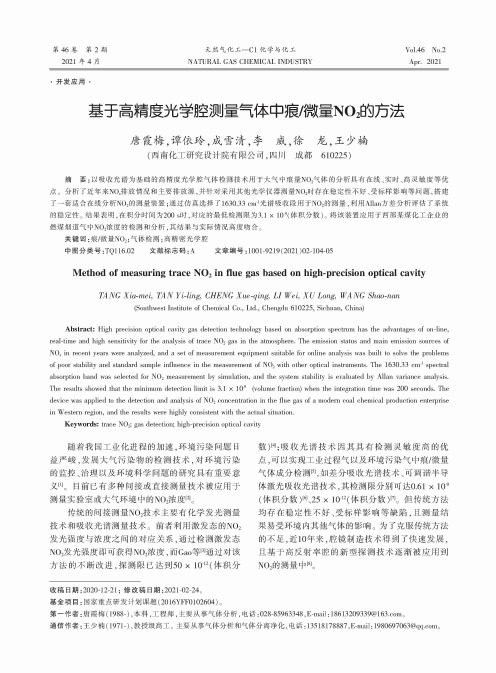
第46卷第2期 2021年4月天然气化工一C1化学与化工NATURAL GAS CHEMICAL INDUSTRYVol.46 No.2Apr. 2021•开发应用•基于高精度光学腔测量气体中痕/微量NO2的方法唐霞梅,谭依玲,成雪清,李威,徐龙,王少楠(西南化工研究设计院有限公司,四川成都610225)摘要:以吸收光谱为基础的高精度光学腔气体检测技术用于大气中痕量NO。
气体的分析具有在线、实时、高灵敏度等优 点。
分析了近年来NOx排放情况和主要排放源,并针对采用其他光学仪器测量NO2时存在稳定性不好、受标样影响等问题,搭建 了一套适合在线分析N〇2的测量装置;通过仿真选择了 1630.33 cm-1光谱吸收段用于N〇2的测量,利用Allan方差分析评估了系统 的稳定性。
结果表明,在积分时间为200 s时,对应的最低检测限为3.1 x 10鄄9(体积分数)。
将该装置应用于西部某煤化工企业的 燃煤烟道气中N〇2浓度的检测和分析,其结果与实际情况高度吻合。
关键词:痕/微量N〇2;气体检测;高精密光学腔中图分类号:TQ116.02 文献标志码:A 文章编号:1001-9219(2021)02-104-05Method of measuring trace N〇2 in flue gas based on high-precision optical cavity TANG Xia-mei, TAN Yi-ling, CHENG Xue-qing, LI Wei, XU Long, WANG Shao-nan(Southwest Institute of Chemical Co., Ltd., Chengdu 610225, Sichuan, China)Abstract: High precision optical cavity gas detection technology based on absorption spectrum has the advantages of on-line, real-time and high sensitivity for the analysis of trace N〇2 gas in the atmosphere. The emission status and main emission sources of N〇x in recent years were analyzed, and a set of measurement equipment suitable for online analysis was built to solve the problems of poor stability and standard sample influence in the measurement of N〇2 with other optical instruments. The 1630.33 cm-1spectral absorption band was selected for N〇2 measurement by simulation, and the system stability is evaluated by Allan variance analysis. The results showed that the minimum detection limit is 3.1 x 10⁹(volume fraction) when the integration time was 200 seconds. The device was applied to the detection and analysis of N〇2 concentration in the flue gas of a modern coal chemical production enterprise in Western region, and the results were highly consistent with the actual situation.Keywords: trace N〇2; gas detection; high-precision optical cavity随着我国工业化进程的加速,环境污染问题日 益严峻,发展大气污染物的检测技术,对环境污染 的监控、治理以及环境科学问题的研究具有重要意 义[1]。
基于GCN-LSTM_的频谱预测算法

doi:10.3969/j.issn.1003-3114.2023.02.001引用格式:薛文举,付宁,高玉龙.基于GCN-LSTM 的频谱预测算法[J].无线电通信技术,2023,49(2):203-208.[XUE Wenju,FU Ning,GAO Yulong.Spectrum Prediction Algorithm Based on GCN-LSTM[J].Radio Communications Technology,2023,49(2):203-208.]基于GCN-LSTM 的频谱预测算法薛文举,付㊀宁,高玉龙(哈尔滨工业大学通信技术研究所,黑龙江哈尔滨150001)摘㊀要:无线频谱是一项重要的㊁难以再生的自然资源㊂在频谱数据中随着信道的动态变化,各个信道不能建模成规则的结构㊂由于卷积神经网络提取的是规则数据结构的相关性,没有考虑信道动态变化以及各个信道节点之间的相关性影响,基于此研究了基于图卷积神经网络(Graph Convolutional Network,GCN)和长短期记忆(Long Short-TermMemory,LSTM)网络结合的GCN-LSTM 频谱预测模型,并且引入了注意力机制,仿真得到了GCN-LSTM 在正确数据集和有一定错误数据的数据集上的预测性能和算法运行时间㊂结果表明在引入注意力机制后,GCN-LSTM 预测模型的准确性和实时性都得到了提高㊂关键词:频谱预测;图神经网络;LSTM;注意力机制中图分类号:TN919.23㊀㊀㊀文献标志码:A㊀㊀㊀开放科学(资源服务)标识码(OSID):文章编号:1003-3114(2023)02-0203-06Spectrum Prediction Algorithm Based on GCN-LSTMXUE Wenju,FU Ning,GAO Yulong(Communication Research Center,Harbin Institute of Technology,Harbin 150001,China)Abstract :Wireless spectrum is an important and hard-to-regenerate natural resource.Since convolutional neural network extractscorrelation of regular data structure,dynamic changes of channel and the correlation between each channel node are not considered.Therefore,this paper studies a GCN-LSTM spectrum prediction model based on the combination of graph convolution neural network GCN and LSTM network,and introduces an attention mechanism.Simulation results show that the prediction performance and algorithm running time of GCN-LSTM on the correct dataset and the dataset with certain error data.Results show that the accuracy and real-timeperformance of GCN-LSTM prediction model are improved after introducing the attention mechanism.Keywords :spectrum prediction;graph neural network;LSTM;attention mechanism收稿日期:2022-12-29基金项目:国家自然科学基金(62171163)Foundation Item :National Natural Science Foundation of China(62171163)0 引言随着无线通信事业的蓬勃发展,各种接入无线网的智能设备数量迅速增长[1],频谱资源趋于紧缺㊂传统的静态频谱分配方式不适配于需求日渐多样化的频谱环境,出现了大量的 频谱空洞 ,造成了频谱资源浪费㊂为解决频谱利用不足的问题,Mitola 在1999年提出了认知无线电(Cognitive Radio,CR)的概念[2]㊂频谱预测的核心就是挖掘并利用历史频谱数据的相关性特征㊂频谱预测可以分为预测信道的占用情况或者是预测用户的位置和传输功率两大类㊂本文主要针对第一类,即预测信道的占用情况㊂早期研究主要采用例如自回归模型[3]㊁隐马尔可夫模型[4]㊁模式挖掘等传统方法㊂随着神经网络的发展,人们开始将神经网络,比如循环神经网络(Recurrent Neural Network,RNN)[5]和长短期记忆网络(Long Short-Term Memory,LSTM)[6]用于预测,LSTM 网络有效缓解了梯度消失和梯度爆炸现象㊂此外,有很多学者对时频联合域频谱预测展开了研究㊂文献[7]利用频谱的这种相关性提出一种二维频繁模式挖掘算法㊂由于不同地点频谱的使用情况也会有很大不同,因此也有研究将频谱预测的维度扩展到时频空域上㊂文献[8]利用神经网络来进行多维频谱预测的方法研究,提出了LSTM网络和其他神经网络结合的方法进行时频空三维的预测,然而只是提出了想法,并没有实现,算法仍处于仿真阶段㊂图神经网络最早由Gori等人[9]提出㊂GCN广泛用于提取图结构的特征信息,从理论上可以将GCN分为基于谱域和空域两类㊂Bruna等人在2014年提出了第一代GCN[10],定义了图上的卷积方法图结构㊂基于空域的图卷积则没有借助谱图理论,可以直接在空域上操作,非常灵活㊂Petar等人在2018年提出了图注意力网络(Graph Attention Network, GAT)[11],在图卷积网络中使用注意力机制,为图结构中不同的节点赋以不同的权重也就是注意力系数,解决了图卷积神经网络(Graph Convolutional Network,GCN)必须提前知道完整图结构的不足㊂把数据处理成图结构之后,利用图神经网络来学习图结构形式的数据可以更有效地挖掘发现其内部特征和模式,与频谱预测的核心不谋而合,因此可以使用图神经网络来进行频谱预测㊂本文首先分析了频谱预测的特点和发展趋势,说明了频谱预测的重要性和可行性㊂其次,针对频谱预测问题提出了GCN-LSTM模型进行二维时频频谱的预测,采用GCN提取频谱数据的拓扑特征,提取得到频谱数据中的频率相关性之后㊂然后利用LSTM网络进行时间维度动态性特征的提取㊂最后,通过引入注意力机制对GCN-LSTM频谱预测算法进行了改进研究㊂1 基于GCN-LSTM网络的频谱预测问题建模㊀㊀图神经网络可以通过分析研究各个节点的空间特征信息得到既包含内容也包含结构的特征表示,因此在本文中处理频谱数据时,不再是建模成规则的图片,而是建模成如图1所示的图结构㊂图结构中的每个节点代表频谱中的各个信道,信道之间是存在关联的,用图中的边表示,时间维度上的各个信道状态即是各个节点的特征㊂图1㊀频谱建模成图结构Fig.1㊀Spectrum modeling and mapping structure为了提取非欧式拓扑图的空间特征,研究人员利用GCN通过图结构的信息和图中节点的信息提取图的结构特征[12],如图2所示㊂GCN如今已经广泛应用于图数据的研究处理领域[13]㊂图2㊀图神经网络的结构示意图Fig.2㊀Structure diagram of graph neural network对于给定的图G=(V,E),V表示图中的节点集合,假设其长度为N㊂可以用图中的节点V和边E来对图进行定义㊂第二代图卷积GCN公式可以简化成:x G∗gθʈðK k=0θk T k(L~)x㊂(1)㊀㊀由式(1)可以看出,图上的卷积不需要整个图都参与运算,只需捕捉到图上的局部特征,减少了需要训练学习的参数量;并且不再需要对图进行特征分解,避免了特征分解的高昂代价㊂但是由于进行矩阵相乘操作,计算的时间复杂度仍然比较高㊂为了对问题进行简化,Kipf等人在文献[14]中设置K=1,只考虑节点的一阶邻居节点㊂如图3所示,当K=1时,对每个节点的特征进行更新时,不但会考虑各个节点本身的输入特征,还会将各个节点的一阶邻域的邻居节点的输入特征也考虑在内㊂取λmax =2,K =1,得到多层传播的图卷积计算公式:H (l +1)=σD ~-12A ~D ~-12H (l )W (l )(),(2)式中,σ(㊃)为非线性激活函数,A ~=A +I N ,A ~为加上自身属性后的邻接矩阵,D ~=ðjA ~ij 表示邻接矩阵A ~的度矩阵,H (l )为第l 层中图节点特征,H (0)=χ,即输入的特征矩阵,W (l )为第l 层的权重,即可训练的卷积滤波参数㊂图3㊀图卷积计算的简单示意图Fig.3㊀Simple diagram of convolution calculation2㊀增加注意力机制的GCN-LSTM 频谱预测算法2.1㊀GCN-LSTM 网络模型利用信道占用模型产生频谱数据,然后将频谱建模成图,频谱中的各个信道建模成图中的各个节点,在频率上提取信道之间的相关性即是提取节点之间的相关性,用GCN 进行提取,时间上的相关性则由LSTM 进行提取㊂GCN-LSTM 频谱预测算法示意如图4所示,内部结构如图5所示㊂图4㊀GCN-LSTM 模型示意图Fig.4㊀GCN-LSTM modeldiagram图5㊀GCN-LSTM 模型内部结构Fig.5㊀Internal structure diagram of GCN-LSTM model图4中,先将图结构形式的频谱输入GCN,提取其拓扑结构特征(即频率相关性),GCN 的输出Z N t 是已经提取了频率相关性的序列数据;然后将提取频率相关性的Z N t 序列输入进LSTM 网络,提取序列数据的时序相关性;最终通过激活函数的激活得到输出,并与真实的频谱数据利用损失函数衡量比较得到误差㊂Z N t 代表输入数据χt 经过图卷积网络后的数据特征㊂i t ㊁f t ㊁o t 分别代表了输入门(Input Gate)㊁遗忘门(Forget Gate)和输出门(Output Gate)㊂图5所示的χt 代表输入的处理成图结构的频谱数据,节点之间的关联强弱代表信道相关性的强弱㊂GCN-LSTM 预测模型公式如下:i t=σ(W iχ㊃Z Nt +W ih ㊃h t -1+b t )f t =σ(W f χ㊃Z N t +W fh ㊃h t -1+b f )o t =σ(W o χ㊃Z N t +W o h ㊃h t -1+b o )c ~t =g (W c χ㊃Z N t +W ch ㊃h t -1+b c )c t =i t☉c ~t +f t ☉c t -1h t =o t☉h -(c t )ìîíïïïïïïïï㊂(3)2.2㊀增加注意力机制的GCN-LSTM 预测模型注意力机制[15]是关注更重点的信息而忽略一些无关的信息,在GCN-LSTM 模型基础上,加入注意力机制,就是对不同时间步的特征赋予不同的权重㊂Soft Attention 注意力机制示意如图6所示,可以分成三步:一是信息输入h j ;二是注意力系数e ij 的计算,e ij 利用神经网络计算,再利用softmax 函数对e ij 进行归一化得到注意力的分布a ij ;三是利用注意力分布αij 与输入的信息进行加权平均得到输出c i㊂αij =exp(e ij )ðN k =1exp(eik)㊂(4)㊀㊀输出c i 为权重与输入的加权平均:c i =ðN j =1αijh j㊂(5)图6㊀Soft attention 注意力机制示意F i g.6㊀Schematic diagram of Soft Attention mechanism㊀㊀增加了注意力机制的GCN-LSTM 模型网络,如图7所示㊂将GCN-LSTM 的输出作为注意力层的输入,通过一个全连接层,再经过softmax 归一化,计算对时间步的权重即注意力分配矩阵,将注意力分配矩阵和输入数据进行逐元素的相乘即得到注意力的输出㊂图7㊀增加注意力机制的GCN-LSTM 模型示意图Fig.7㊀Schematic diagram of GCN-LSTM model forincreasing attention mechanism3 仿真结果利用信道占用模型,产生了5个信道的频谱数据,时间长度为10000,损失函数选择二分类交叉熵损失函数㊂在实验中,设置GCN 的模型参数为:图卷积网络层数为1,初始学习率为0.001,评价GCN-LSTM 预测算法的性能指标为准确率㊂预测窗口长度为10,隐藏单元数hidden_units 为128,batch_size 为64,迭代次数epoch 为20㊂基于GCN-LSTM 预测算法预测的准确率如图8和图9所示㊂图8㊀GCN-LSTM 模型准确率Fig.8㊀GCN-LSTM modelaccuracy图9㊀增加注意力机制的GCN-LSTM 模型精确率Fig.9㊀Increase the accuracy of GCN-LSTMmodel of attention mechanism二分类交叉熵binary_cross entropy 公式为:loss (y ,y ^)=-1nðni(y i lb(y^i )+(1-y i )lb(1-y ^i )),(6)式中,y i 为真实的值,y^i 为预测的值㊂在基础的GCN-LSTM 模型上增加了注意力机制之后,同样训练20轮之后,准确率从96.89%增长到97.86%,准确率得到了提升,训练时间从10.23s 变为12.69s,网络输出时间从0.13s 变为0.15s,时间基本为原来的1.19倍㊂这是因为增加注意力机制后,训练的参数数量从70020增长为78120,数量增多㊂增加注意力机制确实可以提高GCN-LSTM 模型整体的预测性能,而且性能略平稳一些㊂同时对比在频谱数据出现错误情况下的GCN-LSTM 和增加了注意力机制之后的预测模型的预测性能㊂图10为错误概率为0.05的情况,图11为错误概率为0.1的情况㊂比较无错误㊁错误概率为0.05和0.1时,随着错误概率的增加,准确率会略有下降㊂增加注意力机制后的预测算法比没有增加注意力机制的GCN-LSTM 算法指标提高一点,预测性能更好㊂图10㊀GCN-LSTM 模型错误率为0.05时的准确率Fig.10㊀Accuracy when GCN-LSTM model error rate is 0.05图11㊀GCN-LSTM 模型错误率为0.1时的准确率Fig.11㊀Accuracy when GCN-LSTM model error rate is 0.14 结论本文主要研究了基于GCN-LSTM 的频谱预测算法,采用GCN 和LSTM 复合网络GCN-LSTM 预测模型进行时频频谱预测㊂为了考量不同时间步的重要程度,在GCN-LSTM 预测模型基础上增加了注意力机制来提高预测效果㊂此外,实际数据可能存在错误的情况,对无错误数据和错误数据的情况分别进行了仿真㊂仿真结果表明,GCN-LSTM 方法预测准确率较高,且训练时间和预测时间更短,实时性大大提升㊂另外,增加注意力机制后,预测性能也得到一些提高,时间约是没增加注意力机制时的1.2倍㊂对比数据出现错误的情况下,使用GCN-LSTM 算法的预测性能也在可以接受的范围内㊂参考文献[1]㊀DEHOS C,GONZÁLEZ J L,DOMENICO A D,et -limeter-wave Access Andbackhauling:The Solution to the Exponential Data Traffic Increase in 5G Mobilecommuni-cations Systems [J ].IEEE Communications Magazine,2014,52(9):88-95.[2]㊀MITOLA J,MAGUIRE G Q.Cognitive Radio:MakingSoftware Radios More Personal[J].IEEE Personal Com-munications,1999,6(4):13-18.[3]㊀WEN Z,LUO T,XIANG W,et al.Autoregressive Spec-trum Hole Prediction Model for Cognitive Radio Systems [C]ʊIEEE International Conference on Communications Workshops.Beijing:IEEE,2008:154-157.[4]㊀何竞帆.认知无线电频谱预测算法研究[D].成都:电子科技大学,2019.[5]㊀邢玲.基于递归神经网络的频谱预测技术研究[D].成都:电子科技大学,2019.[6]㊀YU L,CHEN J,DING G.Spectrum Prediction via LongShort Term Memory [C]ʊ20173rd IEEE InternationalConference on Computer and Communications (ICCC).Chengdu:IEEE,2017:643-647.[7]㊀YIN S,CHEN D,ZHANG Q,et al.Mining SpectrumUsage Data:A Large-scale Spectrum Measurement Study[J].IEEE Transactions on Mobile Computing,2012,11(6):1033-1046.[8]㊀周佳宇,吴皓.基于神经网络的多维频谱推理方法探讨[J].移动通信,2018,42(2):35-39.[9]㊀GORI M,MONFARDINI G,SCARSELLI F.A New Modelfor Learning in Graph Domains [C]ʊProceedings 2005IEEE International Joint Conference on Neural Networks.Montreal:IEEE,2005:729-734.[10]BRUNA J,ZAREMBA W,SZLAM A,et al.Spectral Net-works and Deep Locally Connected Networks on Graphs [J /OL].arXiv:1312.6203[2022-12-20].https:ʊ /abs /1312.6203.[11]VELIC㊅KOVIC'P,CUCURULL G,CASANOVA A,et al.Graph Attention Networks[J/OL].arXiv:1710.10903[2022-12-20].https:ʊ/abs/1710.10903.[12]魏金泽.基于时空图网络的交通流预测方法研究[D].大连:大连理工大学,2021.[13]SCHLICHTKRULL M,KIPF T N,BLOEM P,et al.Mod-eling Relational Data with Graph Convolutional Networks[C]ʊEuropean Semantic Web Conference.Heraklion:Springer,2018:593-607.[14]KIPF T N,WELLING M.Semi-supervised Classificationwith Graph Convolutional Networks[J/OL].arXiv:1609.02907[2022-12-20].https:ʊ/abs/1609.02907.[15]UNGERLEIDER L G,KASTNER S.Mechanisms of VisualAttention in the Human Cortex[J].Annual Review ofNeuroscience,2003,23(1):315-341.作者简介:㊀㊀薛文举㊀哈尔滨工业大学硕士研究生㊂主要研究方向:频谱预测㊂㊀㊀付㊀宁㊀哈尔滨工业大学硕士研究生㊂主要研究方向:频谱预测㊂㊀㊀高玉龙㊀哈尔滨工业大学教授,博士生导师㊂主要研究方向:智能通信㊁频谱态势认知㊁智能信息融合㊂。
质谱分析法中英文专业词汇
质谱分析法:mass spectrometry质谱:mass spectrum,MS棒图:bar graph选择离子检测:selected ion monitoring ,SIM直接进样:direct probe inlet ,DPI接口:interface气相色谱-质谱联用:gas chromatography-mass spectrometry,GC-MS 高效液相色谱-质谱联用:high performance liquid chromatography-mass spectrometry,HPLC-MS电子轰击离子源:electron impact source,EI离子峰:quasi-molecular ions化学离子源:chemical ionization source,CI场电离:field ionization,FI场解析:field desorptiion,FD快速原子轰击离子源:fast stom bombardment ,FAB质量分析器:mass analyzer磁质谱仪:magnetic-sector mass spectrometer四极杆质谱仪(四极质谱仪):quadrupole mass spectrometer紫外-可见分光光度法:ultraviolet and visible spectrophotometry;UV-vis 相对丰度(相对强度):relative avundance原子质量单位:amu离子丰度:ion abundance基峰:base peak质量范围:mass range分辨率:resolution灵敏度:sensitivity信噪比:S/N分子离子:molecular ion碎片离子:fragment ion同位素离子:isotopic ion亚稳离子:metastable ion亚稳峰:metastable peak母离子:paren ion子离子:daughter含奇数个电子的离子:odd electron含偶数个电子的离子:even eletron,EE 均裂:homolytic cleavage异裂(非均裂):heterolytic cleavage 半均裂:hemi-homolysis cleavage重排:rearragement分子量:MWα-裂解:α-cleavage 电磁波谱:electromagnetic spectrum光谱:spectrum光谱分析法:spectroscopic analysis原子发射光谱法:atomic emission spectroscopy肩峰:shoulder peak末端吸收:end absorbtion生色团:chromophore助色团:auxochrome红移:red shift长移:bathochromic shift短移:hypsochromic shift蓝(紫)移:blue shift增色效应(浓色效应):hyperchromic effect 减色效应(淡色效应):hypochromic effect 强带:strong band弱带:weak band吸收带:absorption band透光率:transmitance,T吸光度:absorbance谱带宽度:band width杂散光:stray light噪声:noise暗噪声:dark noise散粒噪声:signal shot noise闪耀光栅:blazed grating全息光栅:holographic graaing光二极管阵列检测器:photodiode array detector偏最小二乘法:partial least squares method ,PLS褶合光谱法:convolution spectrometry 褶合变换:convolution transform,CT离散小波变换:wavelet transform,WT 多尺度细化分析:multiscale analysis供电子取代基:electron donating group 吸电子取代基:electron with-drawing group荧光:fluorescence荧光分析法:fluorometryX-射线荧光分析法:X-ray fulorometry 原子荧光分析法:atomic fluorometry分子荧光分析法:molecular fluorometry 振动弛豫:vibrational relexation内转换:internal conversion外转换:external conversion 体系间跨越:intersystem crossing激发光谱:excitation spectrum荧光光谱:fluorescence spectrum斯托克斯位移:Stokes shift荧光寿命:fluorescence life time荧光效率:fluorescence efficiency荧光量子产率:fluorescence quantum yield荧光熄灭法:fluorescence quemching method散射光:scattering light瑞利光:Reyleith scanttering light拉曼光:Raman scattering light红外线:infrared ray,IR中红外吸收光谱:mid-infrared absorption spectrum,Mid-IR远红外光谱:Far-IR微波谱:microwave spectrum,MV红外吸收光谱法:infrared spectroscopy 红外分光光度法:infrared spectrophotometry振动形式:mode of vibration伸缩振动:stretching vibrationdouble-focusing mass spectrograph 双聚焦质谱仪trochoidal mass spectrometer 余摆线质谱仪ion-resonance mass spectrometer 离子共振质谱仪gas chromatograph-mass spectrometer 气相色谱-质谱仪quadrupole spectrometer 四极(质)谱仪Lunar Mass Spectrometer 月球质谱仪Frequency Mass Spectrometer 频率质谱仪velocitron 电子灯;质谱仪mass-synchrometer 同步质谱仪omegatron 回旋质谱仪。
[原创]波谱分析英文翻译
![[原创]波谱分析英文翻译](https://img.taocdn.com/s3/m/d18050c685254b35eefdc8d376eeaeaad1f316f4.png)
Differences in Pulse Spectrum Analysis Between Atopic Dermatitis and Nonatopic Healthy ChildrenAbstractObjectives: Atopic dermatitis (AD) is a common allergy that causes the skin to be dry and itchy. It appears at an early age, and is closely associated with asthma and allergic rhinitis. Thus, AD is an indicator that other allergies may occur later. Literatures indicate that the molecular basis of patients with AD is different from that of healthy individuals. According to the classics of Traditional Chinese Medicine, the body constitution of patients with AD is also different. The purpose of this study is to determine the differences in pulse spectrum analysis between patients with AD and nonatopic healthy individuals.Methods: A total of 60 children (30 AD and 30 non-AD) were recruited for this study.A pulse spectrum analyzer (SKYLARK PDS-2000 Pulse Analysis System) was used to measure radial arterial pulse waves of subjects.Original data were then transformed to frequency spectrum by Fourier transformation. The relative strength of each harmonic wave was calculated. Moreover, the differences of harmonic values between patients with AD and non-atopic healthy individuals were compared and contrasted.Results: This study showed that harmonic values and harmonic percentage of C3 (Spleen Meridian, according to Wang’s hypothesis) were significantly different. Conclusions: These results demonstrate that C3 (Spleen Meridian) is a good index for the determination of atopic dermatitis. Furthermore, this study demonstrates that the pulse spectrum analyzer is a valuable auxiliary tool to distinguish a patient who has probable tendency to have AD and/or other allergic diseases.IntroductionAtopic dermatitis (AD) is a common pruritic chronic inflammatory allergic disease. Approximately 10% of all children in the world are affected by atopicdermatitis,typically in the setting of a personal or family history of asthma or allergic rhinitis. It occurs in infancy and early childhood. Sixty percent (60%) of the symptoms manifest in the first year of life, and 85% by 5 years of age. Early onset and close association with other atopic conditions, such as asthma and allergic rhinitis, make atopic dermatitis an excellent indicator that other allergies may occur later.A number of observations suggest that there is a molecular basis for atopic dermatitis; these include the findings of genetic susceptibility, immune system deviation, and epidermal barrier dysfunction. Moreover, according to the classics of Traditional Chinese Medicine, the body constitution of atopic dermatitis patients was also different. Establishment of scientific methods using pulse diagnosis will assistthe diagnosis and follow-up of AD."Organs Resonance"brought up by Wei-Kung Wang provided a scientific explanation for "pulse condition" and "Qi." Organs, heart, and vessels can produce coupled oscil-lation, which minimize the resistance of blood flow, resulting in better circulation. The changes of radial arterial pulse spectrum can reflect the harmonic energy redistribution of a specific organ. Several of the previous studies demonstrate that variations in the harmonics of pulse spectrum can be used in many fields, including diseases, acupuncture,Chinese herbal medications and clinical observation. The new method offers an extraordinary vision of medical investigation by combining pulse spectrum analysis with Traditional Chinese Medicine as well as modern medicine. Wang proposed that the peak values of numbered harmonics might be the representations of each visceral organ,C1 for Liver, C2 for Kidney, C3 for Spleen, etc.Materials and MethodsSubjectsIn total, 60 children (3–15 years of age), comprising 30 with AD (AD group) and 30 nonatopic healthy (non-AD group),participated in the study. The diagnosis of AD was based on the criteria defined by the United Kingdom working party.Nonatopic healthy was defined as those who had no known health problems and no personal or family history of allergic diseases, such as asthma, allergic rhinitis, etc.The experiment protocol was approved by the Institutional Review Board of China Medical University (approval number: DMR97-IRB-087). The written informed consents were obtained from the parents of all participants before they enrolled in this study.Children with a history of major chronic diseases, such as arrhythmia, ardiomyopathy, hypertension, diabetes mellitus, chronic renal failure, hyperthyroidism, difficult asthma,malignancy, and so on were excluded from this study.Those who suffered from any acute disease (e.g., acute upper airway infection or acute gastroenteritis in recent 7days), were also excluded from this experiment. Radial arterial pulse testA pulse spectrum analyzer (SKYLARK PDS-2000 Pulse Analysis System, approved by Department of Health, Executive Yuan, R.O.C. [Taiwan] with a license number 0023302) was used to record radial arterial pulse waves. The pressure transducer of the pulse spectrum analyzer detected artery pressure pulse with 100-Hz sampling rate and 25mm/ sec scanning rate. The output data were stored in digital form in an IBM PC. The subjects were asked to rest for 20 minutes prior to pulse measurements. All procedures were performed in a bright and quiet room with a constant temperature of 258C–268C. Pulses were recorded during 3:00 pm–5:00 pm to avoid the fasting or ingestion effect.Data processingWe transformed original data to spectrum data by Fourier transform as Wang et al described earlier.Briefly, original data were stored as time-amplitude. Mathematics software Matlab 6.5.1 (The MathWorks Inc.) provided Fast Fourier Transformation (FFT) technique to transform time-amplitude data to frequency-amplitude data. Then regular isolated harmonic in a multiple of fundamental frequency appeared.Thefinding gave a spectrum reading up to the 10th harmonic (Cn, n¼0–10). Intensity of harmonics above the 11th became very small and was neglected. Thereafter, the relative harmonic values of each harmonic were calculated ac-cording to Wang’s hypothesis.Harmonic percentage of Cn was defined asStatistical analysisThe experimental data were analyzed by Statistical software SPSS 13.0 for Windows (SPSS Inc.). Comparisons of the harmonic values and the harmonic percentage and the agedistribution between patients with AD and nonatopic healthy individuals were performed using the Student's two samples t test. Comparisons of the sex distribution between patients with AD and nonatopic healthy individuals were performed using the X2 test. Comparisons of the harmonic values and the harmonic percentage between left hand and right hand were performed using the Student's pairedsamples t test. All comparisons were two-tailed, and p<0.05 was considered to be statistically significant.ResultsIn total, 60 children (30 AD and 30 non-AD) participated in the study. The average age of the 60 subjects is 8.02+2.95 years. Baseline characteristics of all participants are shown in Table 1. There is no significant difference in age and gender between the two groups.Relative harmonic values of right radial arterial pulse spectrum analysis are shown in Table 2. Relative harmonic values of left radial arterial pulse spectrum analysis are shown in Table 3. Harmonic percentages of right radial arterial pulse spectrum analysis are shown in Table 4. Harmonic percentages of left radial arterial pulse spectrum analysis are shown in Table 5.In this study, the relative harmonic values of both right and left radial arterial pulse spectrum analysis are lower in the AD group. The relative harmonic values of C3 are significantly different ( p¼0.004, 0.059, respectively). Moreover, when comparingthem by parameter of harmonic percent age, C3 are significantly decreased in the AD group in both right and left radial arterial pulse spectrum analyses ( p¼0.045, 0.036, respectively). These results illustrated the close relationship between C3 (Spleen Meridian) and AD.DiscussionAccording to the theory of Traditional Chinese Medicine,the pathophysiologic mechanisms of AD are "inborn deficiency in body constitution, poor tolerance to environmental stimulants, Spleen Meridian not working well, interiorly generating wet and heat; infected with wind-wetness-heat-evil further, then suffering from those accumulating in skin." AD is a disease involving multiple dysfunctions of the visceral organs (Zang-Fu) rather than a constitutive skin defect.‘‘Spleen wetness’’ is usually considered a major syndrome of AD, which is compatible wi t h our findi n gs.On the other hand, there are also differences in C0 (Heart Meridian), C1 (Liver Meridian), C4 (Lung Meridian) of right hand ( p¼0.014, 0.005, 0.021, respectively) and C1 (Liver Meridian) of left hand ( p¼0.038) between the two groups.These findings appear to have a close relationship between AD and other visceral organs (Zang-Fu). It requires further research to clarify the clinical meanings of these differences.In the present experiment, the close relationship between C3 (Spleen Meridian, referred toWang’s hypothesis) and AD is illustrated. The result verifies Wang’s hypothesis about the relationship between harmonics and Meridians. Moreover,our experiment also has proved that the pulse spectrum analyzer is a suitable auxiliary tool for diagnosing and following up patients with AD.ConclusionsIn conclusion, it was determined that C3 (Spleen Meridian) is a valued index for the determination of atopic dermatitis. Also, the pulse spectrum analyzer is a practi c al noninvasive diagnostic tool to allow scientific and objecti v e di a gnosi s.However, the pulse diagnosis technique is just in the beginning stage. Even though the discovery from the present study seems clear, it deserves further study. AcknowledgmentsThis research was performed in a private clinic for pediatrics specialty, the Hwaishen clinic. The Hwaishen Clinic is acknowledged for their full support of this research. Disclosure StatementNo competing financial interests exist.。
基于两种方法的天气雷达谱宽估算质量比较与改进

第39卷第3期 2016年9月气象与减灾研究Meteorology and Disaster Reduction Research Vol.39 N o.Sept. 2016何田勇,胡明宝,张振仟,等.2016.基于两种方法的天气雷达谱宽估算质量比较与改进[].气象与减灾研究,39(3)216-223.H c T i a n y o n g,H u Mingbao, Zhang Zhcnqian,ct al 2016. Quality comparison and improvement of weather radar spectrumwidth estimation based on two mcthocls[J]. Meteorology and Disaster Reduction Research,39(3) :216-223.基于两种方法的天气雷达谱宽估算质量比较与改进何田勇\胡明宝12,张振仟\艾未华\孟鑫11解放军理工大学气象海洋学院,江苏南京2111012.南京气象雷达开放实验室,江苏南京210008摘要:采用F F T算法和P P P算法,对南京S波段双线偏振全相参脉冲多普勒天气雷达一次实测回波时域/Q信号进行谱宽估计,并对谱宽估计值及其偏差与信噪比的关系进行了分析。
结果发现:)相对高信噪比数据,低信噪比回波的谱宽估计偏差更大,且随信噪比降低偏差呈指数增长。
相对F F T算法,P P P算法的谱宽估计偏差更大,且随信噪比降低偏差增长速度更快。
2)为提高谱宽估计精度必须要尽量消除噪声(主要是低信噪比回波信号)造成的影响,分别对F F T算法和P P P算法提出了改进方案,两种算法的谱宽估计质量都有了较大提升,尤其是低信噪比回波数据。
修正后F F T算法处理得到的谱宽数据与R V P8偏差更小,而修正后P P P算法处理得到的谱宽数据偏差较大且比较离散,这表明F F T算法的估计精度更高,但实际处理过程中P P P算法的处理速度更快,两种谱矩估计算法各有优劣。
- 1、下载文档前请自行甄别文档内容的完整性,平台不提供额外的编辑、内容补充、找答案等附加服务。
- 2、"仅部分预览"的文档,不可在线预览部分如存在完整性等问题,可反馈申请退款(可完整预览的文档不适用该条件!)。
- 3、如文档侵犯您的权益,请联系客服反馈,我们会尽快为您处理(人工客服工作时间:9:00-18:30)。
Some Problems in Application of Information Spectrum Method and Resonant Recognition Model for Cross-spectral Analysis of DNA/RNA SequencesVladimir B.Baji´c1and Ivan V.Baji´c21Centre for Engineering Research,Technikon Natal,P.O.Box953,Durban4000,South Africa E-mail:bajic.v@umfolozi.ntech.ac.za 2University of Natal,Department of Electronic Engineering,King George V Avenue,Durban4001,South AfricaAbstract-The Information Spectrum Method(ISM)and the Resonant Recogni-tion Model(RRM)represent a methodology based on signal processing that analyses char-acteristic spectral motifs in DNA/RNA and protein sequences.Some inconsistencies have been reported recently with regard to the spectral characterization of speciÞc biological sequences utilizing the ISM(RRM)and this motivated examination of the basics of the ISM(RRM).This note provides some discus-sions on the methodology on which the ISM and RRM are based and shows a potential reason why the ISM and the RRM produce inaccurate and unreliable results.Two ex-amples are given to backup the analysis and discussion.I.IntroductionIn the last13years a conceptually interesting methodology for the analysis of DNA/RNA and protein sequences,named initially the Information Spectrum Method(ISM)[1],[2],[3],has been devel-oped.In order to better correspond to the hypothet-ical selective resonant interaction of biomolecules, and after some further development,it was later re-named the Resonant Recognition Model(RRM)[4], [5].This theory treats biological sequences asÞnite length digital signals and attempts to apply meth-ods of signal processing to extract relevant spectral information from these signals.Utilizing the methodology proposed for the ISM (RRM),some inconsistencies have been reported in [6]with regard to the spectral characterization of speciÞc biological sequences.This gave rise to inter-est in examining the foundation of the ISM(RRM) which relates to signal processing and toÞnd pos-sible reasons for the discrepancy in results.In this note discussion of the background of the ISM(RRM) related to the utilization of spectral analysis is given.It is shown why,in the opinion of the authors,the ISM(RRM)will virtually always produce mislead-ing results.The discussion is supported by two ex-amples.II.ISM and RRMThe ISM(RRM)considers biological sequences (DNA/RNA and proteins)asÞnite length signals.DNA/RNA are sequences composed of only4dif-ferent types of nucleotides,while proteins are se-quences composed of20different types of amino-acids.Hence,in their conversion to the form suit-able for the application of signal processing,speciÞc numbers are allocated to each of the nucleotides and each of the amino-acids.This is normally done by means of the so-called Electron-Ion Interaction Po-tential(EIIP)which correlates some physical char-acteristics of nucleotides and amino-acids and some biological properties of organic molecules[7].These numerical values are precalculated and can be found in[4].After assigning the relevant EIIP values to the elements of biological sequences,they become simply numerical sequences ofÞnite length.From this point on,the extraction of the spectral infor-mational content of a selected group of biologically related sequences may be considered to be an engi-neering problem.The ISM(RRM)theory is aimed atÞnding the spectral characterization,the so-called consensus spectrum,of a group of sequences that have the same or similar type of biological functions.It is not known yet what are all the factors that deter-mine the biological function of a particular sequence.However,it is generally considered that the struc-ture of the sequence is one of the most important factors.Our interest here will be focused only on the structure of the sequence.The basis of the ISM(RRM)is the classical cross-spectral analysis.Because the sequences from one functional group,say promoters,normally have dif-1ferent lengths,the shorter sequences are extended to the length of the longest one in the examined group in order to enable the calculation of cross-spectrum.For this we cite [1],p.338,:”Comparison of sequences of di fferent length is done by padding out the shorter sequences with zeros to the length of the longest sequence before compar-ing the DFT.The padding operation may cause error in de Þning peak frequencies.It is interesting that in almost any group of biologically related sequences,the length of sequences do not vary by much.In the case of the great varying length of signals,component spectra are of a shape such that there is only a minor error resulting by padding operation.”The authors of this note are of the opinion that this is not correct in the context of the cross-spectral analysis of biological sequences.In what follows we will restrict our consideration only to the DNA/RNA sequences.For this reason we will refer to the biological sequences as genetic sequences.We point out that the analogous con-sideration holds for protein sequences.For some more details on the ISM and the RRM we will ex-plain the process of signal processing used in these methods.Let us consider a group Γof s numeri-cal sequences,Γ={y i },i =1,2,...,s,which relate to one speci Þc biological function.These sequences are Þrstly detrended,so that a new set ΓD of de-trended sequences {x i }is obtained.Let the longest sequence in ΓD be x L with the length N .Due to di fferent lengths of x i -s all those sequences x i that are shorter than x L are padded by zeros up to the length of x L in order to make a set of sequences of the same length so as to provide the possibility of calculating their cross-spectrum.Then the discrete N points Fourier transform (DFT)is computed for each of the sequences.If X i (n ),n =0,1,...,N −1,is the DFT of x i ,then the consensus magnitude spectrum of all sequences from ΓD is obtained asS (n )=s Yi =1|X i (n )|.The consensus spectrum is nor-malized with regards to frequency by assuming that the distance between the nucleotides in DNA/RNA is constant with the distance of d =1in suitably de-Þned units,so that the range of the normalized fre-quencies of non-redundant components in the spec-trum is [0,0.5].The spectrum is also normalized with regards to the spectral components magnitude,so that the maximal magnitude is of size 1.We will discuss only the magnitude consensus spectrum since it is considered relevant for the ISM (RRM)cross-spectrum calculation.After analyzing a number of functional groups of biological sequences by the above mentioned proce-dures,it is hypothesized in [1],[4],[5],for a num-ber of such groups,that each group in its consen-sus spectrum contains only one su fficiently sig-ni Þcant characteristic frequency component,which is unique for the group,but di ffers from group to group.In the ISM and the RRM a frequency component with the magnitude M is con-sidered signi Þcant if M ≥m,where m is the mean value of components in the consensus spectrum [4].The ISM (RRM)theory proposed is attractive and,if proved,will lead to the interesting implication that many of the biological functions are character-ized by one speci Þc frequency each in the normalized spectrum.However,applying this methodology in [6]to a group of promoter sequences,it was found that di fferent subsets of the same promoter region set have mutually di fferent characteristic frequen-cies,which were also di fferent from the characteris-tic frequency of the whole group.This necessitated the examination of the basics of the ISM and the RRM,the results of which are shown in the next sections.III.Problem backgroundThe signals (numerical sequences)obtained from the genetic sequences are discrete,have Þnite length,and the magnitudes of signal components take val-ues from two well de Þned sets S n and S a with Þnite number of elements each (the set S n has 4elements representing the values of EIIP for nucleotides,while the set S a has 20elements representing the EIIP val-ues for amino acids).The domain D of de Þnition of a genetic sequence s is Þnite and strictly discrete and is de Þned by D ={kd },where k =1,2,...,n,and d is the distance between the nucleotides in DNA/RNA (or the distance of neighboring amino acids in proteins).In the cross-spectral analysis of DNA/RNA se-quences,one of the main problems is that of com-paring the spectra of two Þnite-length sequences of di fferent lengths.Consider the sequences x 1(n ),n =0,1,...,N 1−1,of length N 1and x 2(n ),n =0,1,...,N 2−1,of length N 2,such that N 1<N 2.If X 1(k )and X 2(k )are the DFTs of x 1and x 2,respec-tively,then their respective domains of de Þnition in the normalized spatial frequency domain,are given byS 1={k/N 1|k =0,1,...,N 1−1}S 2={k/N 2|k =0,1,...,N 2−1}To make a meaningful comparison of the two spectra possible,as well as to compute the cross-spectrum of these two sequences,the sets S 1and S 2have to be the same.One possible way to achieve this is by extending the shorter sequence x 1by adding N 2−N 1components to its end,i.e.to create a sequencex (e )1(n )=½x 1(n ),n =0,1,...,N 1−1e (n ),n =N 1,...,N 2−12where e(n)denotes the extension.Suitable choice of e(n)will ensure that x(e)1retains all the signiÞcant characteristics of x1while at the same time mini-mizes the errors introduced by extension.Severalforms of extension,such as periodic,zero-padding,symmetric,etc.,are widely used in variousÞelds ofsignal processing[11].However,with any such ex-tension we also introduce(implicitly)the assump-tion that the new sequence will retain the samebiological function.Otherwise,Þnding the cross-spectrum to characterize a group of functionally re-lated sequences would lose meaning.Although ourproblem is analysis in the spectral domain,the al-terations that may be introduced to the form ofthe original sequence,to make the spectral analysismore convenient,are not allowed if the interpreta-tion of the biological functionality of the sequenceis to be retained.Any assumption about the na-ture(behavior)of the biological sequence s out ofthe original domain D of its deÞnition,which in-cludes also the points in between the known signalcomponents,is not correct.If we assume that thegenetic sequence s is altered in any way by adding to it new components for whatever reason,this im-plies the change of the domain D of deÞnition of thesequence.However,as soon as the original domainD of the sequence is changed,its original biologicalfunction is not guaranteed,i.e.it is most probablethat the new sequence will not have the same or even similar biological function,or it may not have anyparticular biological function at all.ISM(RRM)methodology proposes the zero-padding extension of the shorter sequence,i.e.e(n)=0,n=N1,...,N2−1,using the argument that the value of the EIIP is indeed zero outside ofthe original biological sequence.While this argu-ment might seem to be plausible for isolated biolog-ical sequences such as proteins(although it may bequestioned in view of the protein’s changing envi-ronment),it certainly cannot hold for segments of the DNA/RNA sequence,as they are not isolated from the rest of the DNA/RNA.We will show that there would be no use in making zero-padding for shorter sequences,since errors introduced by this operation might signiÞcantly modify theÞnal result of the cross-spectral analysis.IV.Effects of zero-paddingZero-padding operation is usually used to improvethe visual(or computational)resolution of the spec-trum.It enables the evaluation of the DFT at agreater number of points in the frequency domain than is allowed by the original length of the sig-nal.In view of the discussion in the preceding sec-tion,it would allow the calculation of the spectrum of the signal x1with resolution of1/N2instead of 1/N1,which is the physical resolution dictated bythe length of x1.However,due to the fundamental limitations summarized in the uncertainty principle of Fourier analysis[12],zero-padding by itself can-not improve the quality of the spectral estimate.It merely provides a way of interpolation in the fre-quency domain and,in the absence of any knowledge about the behavior of the signal outside its original domain of deÞnition(as in our case),we cannot de-termine whether or not the interpolation is done on the correct curve.Examples are given in[13]and[14]to show that zero-padding cannot help resolvetwo frequency components whose separation in the frequency domain is less than the limit set by the physical resolution,implying that in such cases it is of little use.The problem is further complicated by the fact that spectra obtained by zero-padding the shorter sequences in ISM(RRM)analysis are being multi-plied in the calculation of the cross-spectrum.Since zero-padding enforces the frequency domain convo-lution of the original frequency components with the rectangular window function W R,it creates signiÞ-cant’noise’sidelobes in regions between the original spectral components(the term’noise’is used in the context of the previous paragraph,to indicate that we cannot determine the exact shape of the spec-trum in these regions).In the example of the pre-vious section,each component of X1(k),when con-volved with W R,would add some’noise’to each of the intervals(k/N1,(k+1)/N1),k=0,1,...,N1−2.’Noise’contribution from each speciÞc component of X1(k)may be relatively insigniÞcant,but the com-bined effect of’noise’produced by all original spec-tral components may easily result in the creation of’noise’components that are of the same order of magnitude or higher than the average of X1(k),as will become obvious from the example in the fol-lowing section.All of these newly created spectral ’noise’components,for whose existence there is no support in the original spectrum of the signal x1, now enter the process of cross-spectral multiplica-tion,and become candidates to be recognized as fre-quency components common to signals x1and x2.Eventually this may lead to obtaining a characteris-tic frequency of a genetic sequence that is a product only of the spectral’noise’components.V.ExamplesA.Example1Let us assume that we want toÞnd the frequency that characterizes the common biological function of a group of sequences that include only sequences whose length is at most32.Let us also assume that two hypothetical biological sequences,x1and x2, each of length32,whose respective spectra are given in Fig.1,belong to the group.Each spectrum in3Figure1—Magnitude spectra of sequence x1and x2 Figure2—Magnitude spectra of zero-padded se-quences x1p and x2p,and their cross-spetrum ob-tained with512points DFThas only3non-zero components.It is easy tothat the cross spectrum of x1and x2is identi-zero,and thus the cross-spectrum of the wholewill yield only components of zero magni-Consequently,the frequency to characterize common biological function of these sequences be found(or,in the worst case,one of the x1or x2does not possess the expectedfunction of the group).Let us now as-that a new sequence x3of the length512isthat has the same biological function as the in the examined group.If it was known that such a sequence exist it would be in-into the cross-spectrum calculation.So,wethe process of cross-spectrum determination consider only the cross-spectrum of x1,x2and .According to the ISM(RRM),zero-padding ofand x2has to be done up to the length of512the new sequences obtained in this way are de-as x1p and x2p.The envelope of the respec-spectra for x1p and x2p,as well as the envelopetheir cross-spectrum are given in Fig.2.As canexpected,the cross-spectrum of zero-padded se-produced a lot of spectral components that not exist in the original cross-spectrum of x1 and x2.These new components can inßuence sig-niÞcantly theÞnal cross-spectrum.Moreover,the strongest spectral components in the cross-spectrum Fig.2are not on the frequency positions of the components of the spectra for x1and x2 in Fig.1.Thus the inconsistency.Example2set of40human promoter sequences was extracted GenBank and EMBL databases.Promoter re-lengths varied from87to606.The sequencesthen divided into several groups according Ta-1.Groups A and B are distinct subsets of the originalof sequences,sorted according to length.Group was formed by combining some of the sequences group A with some of the sequences from groupwhile group D was formed by combining all of the from groups A and B.In groups B,C and the longest sequence is of length606.We applied the ISM(RRM)procedure to groupsC andD from Table1.The resulting consensusare shown in Figs.3-5.Results are summa-in Table2.The results obtained show that the calculatedf RRM varies signiÞcantly depending on the selectionof sequences included in the analysis.Characteris-tic frequencies f RRM obtained for different groups of sequences differ by an amount much larger than the computational resolution of the spectrum in each 4Group No.of seq.Length Rounded av.length A 16≤200141B 24200−650348C 10<650300D40<650265Table 1.Four groups of sequences from theset of 40sequencesGroup f RRM SNR Comp.res.B 0.0604141.241.65×10−3C 0.085885.961.65×10−3D 0.0099151.681.65×10−3Table 2.Results of ISM (RRM)analysis for three groups of sequencesin group BFigure 4—RRM consensus spectrum for sequences in group CFigure 5—RRM consensus spectrum for sequences in group Dcase.SNR in each group is found to be larger than 20,which is the minimal value con-to be signi Þcant.Moreover,in each of the examined shorter sequences are zero-padded length of 606what is the length of the longest in the group.Thus,any of the frequencies can,according to the ISM (RRM),be con-as a characteristic RRM frequency for the set of sequences.The problem,however,is all these f RRM are di fferent and hence unus-for the characterization of the selected group.obvious discrepancy appears and the authors of the opinion that it is due to the e ffects on the content of spectra of individual zero-padded C.Commentsexamples are made only for the illustration pur-to directly point out some problems in cross-calculation if its determination is based on of shorter genetic sequences.We also our opinion on the request that the original of genetic sequence de Þnition must not be due to the demands for the convenience of analysis.conclusion based on these examples is that other techniques have to be developed to han-the problem of cross-spectrum calculation for ge-sequences in a consistent and physically inter-manner.One such technique based on the of ’blurred’spectrum that is suitable for the of biological sequences has been proposed in [10],[8],and has been successfully applied to the problem of promoter region recognition in [8]and [9].5VI.ConclusionsThe examples presented show without doubt that the concept of padding by zeros of shorter sequences in the ISM(RRM)method for the convenience of calculation of the cross-spectrum of different length sequences produces results that may be misleading. At the same time,the biological interpretation of the zero-padded sequences is destroyed.For this reason, such technology of cross-spectrum determination for genetic sequences cannot be accepted.References[1]V.Veljkovi´c,I.´Cosi´c,B.Dimitrijevi´c and D.Lalovi´c,Is It Possible to Analyze DNA and Pro-tein Sequences by the Methods of Digital Signal Processing,IEEE Transactions on Biomedical Engineering,Vol.BME-32,No.5,pp.337-341, May1985.[2]I.´Cosi´c,D.Neši´c,M.Pavlovi´c and R.Williams,Enhancer binding proteins predicted by infor-mational spectrum method,Biophys.Biochem.m.,Vol.141,pp.831-839,1986. [3]I.´Cosi´c,M.Pavlovi´c and V.Vojisavljevi´c,Pre-diction of’hot spots’in interleukin-2based on informational spectrum characteristics of growth regulating factors,Biochimie,Vol.71, pp.333-342,1989.[4]I.´Cosi´c,Macromolecular Bioactivity:Is It Res-onant Interaction Between Macromolecules?-Theory and Applications,IEEE Transactions on Biomedical Engineering,Vol.41,No.12, pp.1101-1114,December1994.[5]I.´Cosi´c,The Resonant Recognition Model ofMacromolecular Bioactivity-Theory and Ap-plications,Birkhäuser,1997.[6]V.B.Baji´c,I.V.Baji´c and W.Hide,Appli-cation of Resonant Recognition Model to a set of human promoters:A word of warning,to appear in Proceedings of the International Sys-tems,Signals,Control,Computers(SSCC’98) Conference,Durban,South Africa,1998. [7]V.Veljkovi´c and I.Slavi´c,General models ofpseudo-potentials,Phys.Rev.Lett.,Vol.29, pp.105-108,1972.[8]V. B.Baji´c,I.V.Baji´c and W.Hide,Ad-vantages and drawbacks of spectral analysis of DNA sequences,Plenary Lecture,to appear in Proceedings of The First International Confer-ence on Bioinformatics of Genome Regulation and Structure,(BGRS’98)Novosibirsk,Russia, 1998[9]V.B.Baji´c,I.V.Baji´c and W.Hide,Spec-tral characterization of human promoters,toappear in Proceedings of the International Sys-tems,Signals,Control,Computers(SSCC’98)Conference,Durban,South Africa,1998.[10]V.B.Baji´c and I.B.Baji´c,Spectral meth-ods for analysis of DNA/RNA and protein se-quences,Technical Report,Technikon Natal,1998.[11]G.Strang and T.Nguyen,Wavelets andÞlterbanks,Wellesley-Cambridge Press,Wellesley,MA,USA,1996.[12]A.Papoulis,Signal Analysis,McGraw-HillBook Company,New York,1977.[13]J.G.Proakis and D.G.Manolakis,Digital Sig-nal Processing:Principles,Algorithms and Ap-plications,Second Ed.,Macmillan PublishingCompany,New York,1992[14]S.J.Orfanidis,Introduction to Signal Process-ing,Prentice Hall,Upper Saddle River,NewJersey,1996.6。