Isospin breaking in scalar and pseudoscalar channels of radiative $Jpsi$-decays

合集下载

Quantum Mechanics

Quantum MechanicsQuantum mechanics is a fascinating and complex field of physics that has revolutionized our understanding of the universe at the smallest scales. At its core, quantum mechanics deals with the behavior of particles at the quantum level, where the classical laws of physics break down and give way to a whole new set of rules. This field has given rise to many groundbreaking theories and technologies, such as quantum computing and quantum cryptography, that have the potential to revolutionize the way we live and interact with the world around us. One of the key principles of quantum mechanics is the concept of superposition, which states that a particle can exist in multiple states simultaneously until it is observedor measured. This idea challenges our classical intuition, which tells us that an object can only be in one place or state at a time. The famous thought experiment known as Schr?dinger's cat illustrates this concept, where a cat in a box is both alive and dead until the box is opened and the cat is observed. This idea of superposition has profound implications for the nature of reality and has led to many thought-provoking philosophical debates about the nature of existence. Another important concept in quantum mechanics is entanglement, where twoparticles become interconnected in such a way that the state of one particle is directly linked to the state of the other, regardless of the distance between them. This phenomenon, famously referred to as "spooky action at a distance" by Albert Einstein, challenges our understanding of causality and suggests that particlescan communicate instantaneously with each other, defying the limitations of space and time. This idea has been experimentally verified through a series of groundbreaking experiments and has opened up new possibilities for quantum communication and teleportation. The implications of quantum mechanics extend far beyond the realm of theoretical physics and have the potential to revolutionize technology in ways we can only begin to imagine. Quantum computing, for example, harnesses the principles of superposition and entanglement to perform calculations at speeds that far surpass classical computers. This has the potential to revolutionize fields such as cryptography, drug discovery, and artificial intelligence, unlocking new possibilities for innovation and discovery. Similarly, quantum cryptography uses the principles of quantum mechanics to create securecommunication channels that are theoretically impossible to hack, offering a new level of security and privacy in an increasingly digital world. Despite the incredible potential of quantum mechanics, there are still many challenges and mysteries that remain to be solved. The field is notoriously complex and counterintuitive, with many of its fundamental principles defying our classical understanding of the world. This has led to many debates and disagreements among physicists about the true nature of quantum mechanics and how best to interpretits implications. The famous Copenhagen interpretation, for example, posits that particles exist in a state of superposition until they are observed, while the many-worlds interpretation suggests that every possible outcome of a quantum event actually occurs in a separate parallel universe. These differing interpretations highlight the deep philosophical questions that quantum mechanics raises about the nature of reality and our place in the universe. In conclusion, quantum mechanics is a field that continues to push the boundaries of our understanding of the universe and challenge our most deeply held beliefs about the nature of reality. Its principles of superposition, entanglement, and uncertainty have revolutionized our understanding of the quantum world and opened up new possibilities for technology and innovation. While there are still many mysteries and debates surrounding quantum mechanics, its potential to revolutionize fields such as computing, communication, and cryptography is undeniable. As we continue to explore the implications of quantum mechanics, we are sure to uncover even more profound insights into the nature of the universe and our place within it.。

Copy of Echinoderm word

5
Feeding behaviors
• Some echinoderms are ____________, others are detritus foragers (sea cucumbers) or plank tonic feeders (basket stars). • Sea stars are carnivorous and prey on worms or on mollusks such as clams. Most sea urchins are herbivores and gaze on algae. Brittle stars, sea lilies and sea cucumbers feeds on dead and decaying matter that drifts down to the ocean floor.
7
reproduction
• _______ reproduction • A Echinoderm is a male or female. The males and females discharge their eggs and sperm into the water where they are fertilized. • ______ reproduction • Many echinoderms have remarkable powers of regeneration. If a piece of certain echinoderms is chopped off, a new piece or even a new echinoderm can regrow.
3
Echinoderm
• _______________larvae at larval stages • Adult _____________enables animals to sense potential food, predators and other aspects of their environment from direction.

Laser Principle

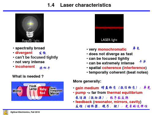
kink in output power 扭结、弯曲
Laser history
Javan invents He-Ne laser Maiman builds first Townes invents and Schawlow and Townes (ruby) LASER builds first MASER propose LASER Spectra introduces first fiber optic communication IBM builds first system Hall buildsAlferov builds first laser printer (Chicago) player Einstein predicts CD Ti:Sapphire laser heterostructure laser semiconductor stimulated emission laser Nakamura builds builds quantum built Faist nanowire laser at UCB blue laser diode cascade laser
Optical Electronics, Fall 2010
Optical Electronics, Fall 2010
Optical Electronics, Fall 2010
Optical Electronics, Fall 2010
Optical Electronics, Fall 2010
laser as amplifier
Input Monitor tap
隔离器
Isolator
隔离器
Isolator Monitor tap Output

翻译

Thermal entanglement in a two-qubit Heisenberg XXZ spin chainunder an inhomogeneous magnetic field 在不均匀磁场作用下的两个量子比特海森堡海森伯 XXZ 自旋链中的热纠缠State Key Laboratory for Superlattices and Microstructures, Institute of Semiconductors, Chinese Academy of Sciences,超晶格、微结构，半导体研究所中国科学院，国家重点实验室P. O. Box 912,Beijing 100083, People’s Republic of China China Center of Advanced Science and Technology (CCAST) (World Laboratory), P. O. Box 8730, Beijing 100080,People’s Republic of China中国中心的先进的科学与技术 (CCAST) (世界实验室)、邮政信箱8730，北京 100080，中国人民共和国Received 15 March 2005; published 2 September 2005The thermal entanglement in a two-qubit Heisenberg XXZ spin chain is investigated under an inhomogeneous magnetic field b. We show that the ground-state entanglement is independent of the interaction of z-component Jz. The thermal entanglement at the fixed temperature can be enhanced when Jz increases. We strictly show that for any temperature T and Jz, the entanglement is symmetric with respect to zero inhomogeneous magnetic field, and the critical inhomogeneousmagnetic field bc is independent of Jz. The critical magnetic field Bc increases with the increasing b but the maximum entanglement value that the system can arrive at becomes smaller.两个量子比特海森堡海森伯 XXZ 自旋链中的热纠缠是根据不均匀磁场 b 进行调查。

Kaons and antikaons in asymmetric nuclear matter

Kaons and antikaons in asymmetric nuclear matter
Amruta Mishra∗ Department of Physics,Indian Institute of Technology, Delhi, New Delhi - 110 016, India Stefan Schramm† and W. Greiner
and its width, which in turn strongly inﬂuence the antikaon-nucleus optical potential, are very sensitive to the many-body treatment of the medium eﬀects. Previous works have ¯ self energy has a strong impact on the shown that a self-consistent treatment of the K scattering amplitudes [14, 20, 22, 23, 24, 25] and thus on the in-medium properties of the antikaons. Due to the complexity of this many-body problem the actual kaon and antikaon self energies (or potentials) are still a matter of debate. The topic of isospin eﬀects in asymmetric nuclear matter has gained interest in the recent past [26]. The isospin eﬀects are important in isospin asymmetric heavy-ion collision experiments. Within the UrQMD model the density dependence of the symmetry potential has been studied by investigating observables like the π − /π + ratio, the n/p ratio [27], the ∆− /∆++ ratio as well as the eﬀects on the production of K 0 and K + [28] and on pion ﬂow [29] for neutron rich heavy ion collisions. Recently, the isospin dependence of the in-medium NN cross section [30] has also been studied. In the present investigation we will use a chiral SU(3) model for the description of hadrons in the medium [31]. The nucleons – as modiﬁed in the hot hyperonic matter – have previously been studied within this model [32]. Furthermore, the properties of vector mesons [32, 33] – modiﬁed by their interactions with nucleons in the medium – have also been examined and have been found to have sizeable modiﬁcations due to Dirac sea polarization eﬀects. The chiral SU(3)f lavor model was generalized to SU(4)f lavor to study the mass modiﬁcation of D-mesons arising from their interactions with the light hadrons in hot hadronic matter in [34]. The energies of kaons (antikaons), as modiﬁed in the medium due to their interaction with nucleons, consistent with the low energy KN scattering data [35, 36], were also studied within this framework [37, 38]. In the present work, we investigate the eﬀect of isospin asymmetry on the kaon and antikaon optical potentials in the asymmetric nuclear matter, consistent with the low energy kaon nucleon scattering lengths for channels I=0 and I=1. The pion nucleon scattering lengths are also calculated. The outline of the paper is as follows: In section II we shall brieﬂy review the SU(3) model used in the present investigation. Section III describes the medium modiﬁcation of ¯ ) mesons in this eﬀective model. In section IV, we discuss the results obtained the K(K for the optical potentials of the kaons and antikaons and the isospin-dependent eﬀects on these optical potentials in asymmetric nuclear matter. Section V summarizes our results and discusses possible extensions of the calculations. 3

Inflation in Realistic D-Brane Models

Contents
1. Introduction 2. Fluxes, Warping and Moduli Fixing 2.1 GKP Compactiﬁcations 2.2 Anti-Branes and Supersymmetry Breaking 2.3 Seeking Slow Rolls 2.4 Sticking the Standard Model in the Throat 3. The Eﬀective Theory 3.1 Supersymmetric Terms 3.2 Supersymmetry-Breaking Terms 4. Inﬂationary Dynamics 4.1 Domain of Validity of Approximations 4.2 Inﬂationary Dynamics 4.2.1 4.2.2 4.2.3 Qualitative Description Numerical Results Scaling Arguments 1 3 3 6 7 8 10 11 13 14 15 16 16 20 24 25 30 30 32 34
The possibility of having cosmological inﬂation arise due to the relative motion of D-branes and their anti-branes is very attractive [1, 2, 3].1 It provides an explicit and
1
See also [4] for an early brane-antibrane proposal which does not rely on the relative inter-brane

98 德国缺陷正电子湮没

Appl.Phys.A66,599–614(1998)Applied Physics AMaterialsScience&Processing©Springer-Verlag1998 Invited paperReview of defect investigations by means of positron annihilationin II−VI compound semiconductorsR.Krause-Rehberg,H.S.Leipner,T.Abgarjan,A.PolityFachbereich Physik,Martin-Luther-Universität Halle-Wittenberg,06099Halle,Germany(Fax:+49-345/5527160,E-mail:krause@physik.uni-halle.de)Received:19November1997/Accepted:20November1997Abstract.An overview is given on positron annihilation stud-ies of vacancy-type defects in Cd-and Zn-related II−VI com-pound semiconductors.The most noticeable results among the positron investigations have been obtained by the study of the indium-or chlorine-related A centers in as-grown cad-mium telluride and by the study of the defect chemistry of the mercury vacancy in Hg1−x Cd x Te after post-growth an-nealing.The experiments on defect generation and annihila-tion after low-temperature electron irradiation of II−VI com-pounds are also reviewed.The characteristic positron life-times are given for cation and anion vacancies.PACS:61.70;78.70BII−VI compound semiconductors are considered for appli-cations in fast-particle detectors and can cover the whole wavelength range from the far infrared to the near ultraviolet in optoelectronic devices.The width of the band gap can be adjusted in pseudo-ternary compounds such as Hg1−x Cd x Te by varying the composition x.The II−VI semiconductors appeared promising for emitter or detector devices because of their excellent optical features together with the pre-dicted favorable transport properties.However,no techno-logical breakthrough has been achieved.This is mainly be-cause no II−VI compound,except CdTe,can be amphoteri-cally doped.Bulk crystals of ZnSe,CdSe,ZnS,and CdS are always n-type,independent of impurities[1].ZnTe appears only as p-type[2].A number of theoretical approaches for this behavior exists but noﬁnal experimental proofs for these theories have been given.The reason for the compensation could be the existence of extrinsic defects introduced during crystal growth.However,intrinsic defects or complexes of in-trinsic defects with dopants have also been discussed.The research on II−VI compounds was greatly stimulated by the growth of nitrogen-doped,p-type ZnSe layers by mo-lecular beam epitaxy(MBE)[3,4].p–n junctions were made, andﬁrst ZnSe-based blue lasers could be fabricated[5,6]. Nevertheless,the doping behavior of nitrogen-doped ZnSe layers is also not fully understood.It is not clear why only the nitrogen doping during MBE works for p-type conductiv-ity and why other epitaxial growth techniques provide hole densities of one order of magnitude lower[7].Obviously,the understanding of point defects in II−VI semiconductors is far from being complete.Vacancy-type defects,for example monovacancies and complexes contain-ing a vacancy,play an important role.A prominent defect in doped CdTe is the A center,identiﬁed by electron para-magnetic resonance measurements as a cadmium vacancy paired off with a dopant atom at the nearest neighbor site[8]. The dominant defect in Hg1−x Cd x Te is the mercury mono-vacancy,acting as an acceptor.A high concentration of V Hg may be the reason for the p-conductivity.These examples show the importance of experimental tools for the detection of vacancy-type defects.Such a method is positron annihila-tion,which was successfully applied for the investigation of the structure and the concentration of such defects in elemen-tal and compound semiconductors[9–11].Signiﬁcant contri-butions have been made by positron annihilation to revealing the structure of such important defects in III−V compounds as the EL2defect and the DX center[12–14].The aim in this paper is to review available experimen-tal data on defect studies in II−VI compounds by positron annihilation.The paper is organized as follows.The relevant methods of positron annihilation spectroscopy and theoretical calculations of the positron lifetime in II−VI compounds are introduced in Sect.1.The experimental results on cadmium mercury telluride,cadmium telluride,and zinc-related II−VI compounds are reviewed in Sect.2.Section3summarizes positron data on irradiation-induced defects.1Basics of positron annihilation in semiconductors1.1Positron lifetime and Doppler-broadening spectroscopy The detection of defects by means of positron annihilation is based on the capture of prehensive treatments of positron annihilation in solids can be found elsewhere[15–18].Attractive potentials for positrons exist for open-volume defects,e.g.vacancies,and for negatively charged non-open600volume defects,e.g.acceptor-type impurities.The potential is based in the latter case only on the Coulomb attraction be-tween the positron and the negative defect[19].The main reason for the binding of positrons to an open-volume defect is the lack of the repulsive force of the nucleus.Additional Coulombic contributions,which enhance or inhibit the trap-ping owing to a negative or a positive charge,respectively, occur for charged vacancies[18].The positrons in a typical conventional positron experi-ment are generated in an isotope source.They penetrate the sample,thermalize and diffuse.They can be trapped in de-fects during diffusion over a mean distance of about100nm. This may result in characteristic changes of annihilation pa-rameters.The positron lifetime for open-volume defects is increased in relation to the undisturbed bulk.This is due to the reduced electron densities in these defects.The clustering of vacancies in larger agglomerates can be observed as an in-crease in the defect-related positron lifetime.The lifetime of a positron is monitored in positron lifetime spectroscopy(PO-LIS)as the time difference between the birth of the particle in the radioactive source,indicated by the almost simultan-eous emission of a1.27-MeVγquantum,and the annihilation in the sample,resulting inγrays with an annihilation energy of0.511MeV.The lifetime spectrum is formed by the col-lection of several million annihilation events.In general,the spectrum consists of several exponential decay components, which can be numerically separated(see Sect.1.3).Doppler-broadening spectroscopy(DOBS),as another positron technique,utilizes the conservation of momentum during annihilation.The total momentum of the positron and the electron is practically equal to the momentum of the annihilating electron.This momentum is transferred to the annihilationγquanta.The momentum component in the propagation direction,p z,results in a Doppler shift of the an-nihilation energy of∆E=p z c/2(where c is the speed of light).The accumulation of several million events for a whole Doppler spectrum in an energy-dispersive system leads to the registration of a Doppler-broadened line,which is caused by the contributions of electron momentums in all space di-rections.The distribution of electron momentums may be different close to defects,and this is reﬂected in characteris-tic changes of the shape of the annihilation line.Annihilations with core electrons having higher momentums are reduced, for example,for a vacancy,and thus the annihilation line be-comes narrower.The annihilation line is usually speciﬁed by shape parameters,such as the S parameter,which is deﬁned as the area of aﬁxed central region of the Doppler peak normal-ized to the whole area under the peak,i.e.to the total number of annihilation events.Another parameter is the W parameter, deﬁned in the wing parts of the annihilation line.This param-eter is determined mainly by the annihilations of the positrons with core electrons.The W parameter is thus more sensitive to the chemical nature of the surrounding of the annihilation site.A plot of the W parameter versus the S parameter may be used for the identiﬁcation of defect types[20,21].The slope of the line corresponds to the R parameter,which is charac-teristic for a certain defect type,independent of the defect concentration.If the pairs of(S,W)values plotted for differ-ent sample conditions lie on a straight line running through the bulk values(S b,W b),one has to conclude that one sin-gle defect type having different concentrations dominates the positron trapping.Positrons from an isotope source have a broad energy dis-tribution of up to several hundred keV.This leads to a mean penetration depth of some10µm,and thin epitaxial layers cannot be studied.Therefore,the slow positron beam tech-nique[22]was developed.It is based on the moderation of positrons,i.e.the generation of monoenergetic positrons with energies in the eV range.The energy of the positron beam can be adjusted in an accelerator stage.This allows the registra-tion of annihilation parameters as a function of the penetra-tion depth.Hence,depth proﬁling is possible with a variable information depth of up to a fewµm.The basics of the defect proﬁling by slow positrons in comparison with other methods was presented by Dupasquier and Ottaviani[23].A main result of the positron experiments is the positron trapping rateκ,which is proportional to the defect concentra-tion C,κ=µC.(1) The proportionality constantµis the trapping coefﬁcient (speciﬁc trapping rate),which must be determined in correla-tion to an independent reference method.The determination of the trapping coefﬁcient for semiconductors has been re-viewed by Krause-Rehberg and Leipner[24].Equation(1) holds strictly only in the case of a rate-limited transition of the positron from the delocalized bulk state into the deep bound state of the defect[18].This case describes well the positron trapping in vacancies.The trapping coefﬁcient for small vacancy clusters(n≤5)increases with the number of incorporated vacancies n,µn=nµv,(2) whereµv is the trapping coefﬁcient of monovacancies[25].1.2Temperature dependence of positron trapping in chargeddefectsThe trapping coefﬁcientµin(1)is always a speciﬁc con-stant for a given temperature.The attractive potential is su-perimposed by a long-range Coulomb potential in the case of a charged defect.A positive charge causes a strong repul-sion of the positron,and trapping is practically impossible.In contrast,a negative charge promotes positron trapping com-pared to a neutral defect by the formation of a series of attractive shallow Rydberg states[26].The positron bind-ing energy to the shallow Rydberg states is of the order of some10meV and,therefore,the enhancement of positron trapping is especially effective at low temperatures,where the positron may not escape by thermal activation.Thus,a dis-tinct temperature-dependent trapping rate was obtained for negatively charged vacancies in Si[27]and in GaAs[28].A detailed description of the temperature dependence of positron trapping in negatively charged vacancies was given by Le Berre et al.[28].Non-open volume defects,such as acceptor-type impuri-ties or negatively charged antisite defects,may also act as positron traps provided that they carry a negative charge.The extended shallow Rydberg states are exclusively responsible for positron trapping.The binding energy of the positron is small and therefore these defects are called shallow positron traps.The positron–position probability density at the defect601 nucleus is vanishingly small because of the repulsion fromthe positive nucleus.Therefore,the positron is located andannihilates in the bulk surrounding the defect.The electrondensity felt by the positron equals the density in the bulkand hence the positron lifetime of the shallow trap is closeto the bulk lifetime.Positron trapping to these shallow trapsis important at low temperatures in practically all compoundsemiconductors.Manninen and Nieminen[29]calculated thetemperature dependence of the positron detrapping rateδ:δ=κCmk B T2πh23/2exp−E bk B T.(3)Here,κand C are the trapping rate and the concentration of the shallow positron traps.m is the effective positron mass,k B the Boltzmann constant,and E b the positron binding energy.The description of the trapping in charged defects shows that in the presence of several charged defect types in the ma-terial the temperature dependence of positron trapping may be rather complex and a quantitative evaluation of the annihi-lation parameters as a function of the temperature T is often not possible.1.3Trapping modelA phenomenological description of positron trapping was given by Berlotaccini and Dupasquier[30]and was later gen-eralized[31,32].The model is referred to as the“trapping model”.The aim is the quantitative analysis of lifetime spec-tra in order to calculate the trapping rates and the correspond-ing defect concentrations.Only one extended model that is sufﬁcient for the interpretation of the experimental results is discussed in this paper.This model(Fig.1)includes two dif-ferent types of non-interacting open-volume defects and one shallow positron trap exhibiting thermal detrapping with the detrapping rateδ.The corresponding differential equations ared n b(t) d t =−(λb+κd1+κd2+κd3)n b(t)+δn d1(t),d n d1(t) d t =−(λd1+δ)n d1(t)+κd1n b(t),d n d2(t) d t =−λd2n d2(t)+κd2n b(t),d n d3(t)d t=−λd3n d3(t)+κd3n b(t).(4)Defect d1is the shallow positron trap,and d2and d3are open-volume defects,such as vacancies and vacancy agglom-erates.b denotes the bulk state.The n i are the normalized numbers of positrons in the state i(i=b,d1,d2,d3)at the time t,andλi are the corresponding annihilation rates(inverse positron lifetimes).The starting conditions are n b(0)=1and n d1(0)=n d2(0)=n d3(0)=0.The solution of(4)is a sum of four exponential decay terms,the prefactors of which are the intensities I1to I4.The lifetimesτ1toτ4are found in the exponents.The lifetimes and intensities are obtained asτ1=2Λ+Ξ,τ2=2Λ−Ξ,τ3=1λd2,τ4=1λd3,andFig.1.Scheme of a trapping model including two types of open-volumedefects,d2and d3,and one shallow positron trap,d1.The latter exhibitsthermally induced detrapping with the temperature-dependent detrappingrateδ.The individual trapping ratesκd1,κd2,andκd3and the correspond-ing annihilation ratesλd1,λd2,andλd3are drawn as arrows.λb is the bulkannihilation rateI1=1−(I2+I3+I4),I2=δ+λd1−12(Λ−Ξ)Ξ×1+κd1δ+λd1−12(Λ−Ξ)+κd2λd2−12(Λ−Ξ)+κd3λd3−12(Λ−Ξ),I3=κd2(δ+λd1−λd2)λd2−12(Λ+Ξ)λd2−12(Λ−Ξ),I4=κd3(δ+λd1−λd3)λd3−12(Λ+Ξ)λd3−12(Λ−Ξ).(5)The abbreviations in(5)areΛ=λb+κd1+κd2+κd3+λd1+δ,Ξ=(λb+κd1+κd2+κd3−λd1−δ)2+4δκd1.(6)The two long-lived lifetimes are equal to the defect-related lifetimes:τ3=τd2andτ4=τd3,and they are inde-pendent of the defect concentrations.The average positronlifetimeτfor this model is given byτ=4j=1I jτj.(7)The result(5)represents the components of the lifetime spec-trum.The experimental spectrum may be decomposed in suchcomponents,and the lifetimes and their intensities can beused to determine the corresponding trapping and detrappingrates.Equation(1)then provides the defect concentrations.Cases where the number of independent defects is smallerthan three can easily be obtained from(5)by setting the cor-responding trapping rates to zero.6021.4Theoretical calculation of positron lifetimesThe positron lifetimes in the bulk and in lattice defects of II −VI compounds were ﬁrst theoretically calculated by Puska [33]who used the linear mufﬁn-tin orbital band-structure method within the atomic sphere approximation.Monovacancies were treated in different charge states by the corresponding Green’s function method.More recent calcu-lations from the same group [34,35]used the superimposed-atom model [36].A supercell approach with periodic bound-ary conditions for the positron wave function retaining the three-dimensional character of the crystal was employed.The electron–positron correlation potential was treated with the local-density approximation (LDA)[37].The results of pure LDA calculations provided lifetimes,which were too low compared to experimental values.The calculation method was hence modiﬁed in such a way that the d-electron en-hancement factors for Zn ,Cd ,and Hg were scaled to provide the correct lifetimes for the pure metals [34,35].Another ap-proach used the enhancement factors for d electrons in Ag and Au [38].Calculations of positron lifetimes of vacan-cies were carried out with unscaled LDA [34,35],providing values that are obviously too small compared to the bulk life-times of the scaled LDA calculations.In order to compare the theoretical defect-related lifetimes to the experimental ones and to the bulk lifetimes (Table 1),the vacancy lifetimes given by Plazaola et al.[34,35]were multiplied by the ratio of the bulk lifetimes calculated for the pure and scaled LDA,respec-tively.No relaxation effects and Jahn-Teller distortions were taken into account in these computations.Although the positron lifetimes for almost all II −VI com-pound semiconductors have been calculated,only materials for which experimental data exist are included in Table 1.The calculated bulk lifetimes agree reasonably well with the ex-perimental values.However,the lifetimes calculated for the vacancies are always distinctly smaller than the measured ones.Table 1.Calculated and experimental positron lifetimes for II −VI semiconductors.The bulk lifetimes were calculated using a modiﬁed semi-empirical local density approximation (LDA)[34,35].The LDA lifetimes for the vacancies given by Plazaola et al.[34,35]are scaled by a factor to allow a more realistic comparison to the experiments (see text).The experimental values of the cation vacancies (vacancies of group II atoms)are related to the A centers in In -or Cl -doped CdTe ,to the mercury vacancies in Hg 1−x Cd x Te ,and to the Zn vacancies as part of complexes in Zn -related compounds,respectively.The only experimental value for anion vacancies (vacancies of group VI atoms)is that of the tellurium vacancy in Hg 1−x Cd x Te MaterialBulk lifetime /psCation-vacancy lifetime /ps Anion-vacancy lifetime /ps Calculated Experimental Calculated Experimental Calculated Experimental CdTe286291[104]298320±5[45,46]312–281[68]330±15[44,52,68]283±1[44]285±1[45,46]280±1[52]HgTe274274[68]285–300–Hg 0.8Cd 0.2Te –274[68]–309[69]–325±5[93]286[69]305[54,70]275[54]319[97]278[70]282[97]ZnO –169±2[88]–255±16[86,87]––183±4[86,87]211±6[102]ZnS 225230[78,80]240290[80]237–ZnSe 240240[79]253–260–ZnTe260266[78]266–297–2Characterization of defects in as-grown II –IV compounds 2.1Cadmium tellurideCadmium telluride can be amphoterically doped.However,the doping and compensation behavior are still not com-pletely understood.Important defects for the understanding of the compensation are the impurity-vacancy complexes called “A centers”[39].These centers consist of a group-II vacancy paired off with either a group-VII donor (F ,Cl ,Br ,I )on the Te site,or with a group-III donor (e.g.Ga ,In )the Cd site [40].The ionization level of the Cl -related A center,(V Cd Cl Te )−/0,was determined by photolumines-cence measurements to be located at 150meV above the va-lence band [41].The levels for the isolated monovacancies were also investigated experimentally.The 2−/−level of the Cd vacancy was found with electron paramagnetic resonance at E d −E v <470meV [42]and the 0/+level of the Te va-cancy (F center)at E d −E v <200meV (E d defect ionization level,E v position of the top of the valence band)[43].2.1.1The A center.Weakly In -doped cadmium telluride was studied by positron lifetime spectroscopy as a func-tion of the temperature [44–46].Distinct positron trapping in a monovacancy-type defect was found.The defect-related lifetime was given ﬁrst as 330±5ps [44],but was corrected later to 320±5ps [45,46].The lifetime was interpreted to be either due to isolated Cd monovacancies in a double negative charge state or due to (V Cd In Cd )−complexes.The average positron lifetime exhibited a distinct decrease with decreasing temperature,which was attributed to the presence of shal-low positron traps,i.e.negatively charged non-open volume defects.The compensation mechanism in iodine-doped CdTe lay-ers grown by MBE was investigated by photoluminescence (PL),conductivity measurements,and Doppler-broadening603spectroscopy [47].The DOBS S parameter increased dis-tinctly with increasing iodine concentration,i.e.with the free-electron concentration.The iodine doping obviously induced vacancy-type defects.This result is in agreement with the proposed microscopic structure of the iodine-related A center [40].Kauppinen and Baroux [48]investigated CdTe crystals doped with In or Cl with positron lifetime and Doppler-broadening spectroscopy.The Doppler measurements were carried out in a background-reducing coincidence setup [49,50].Vacancy-type defects were found in all samples.Defect-related lifetimes of 323and 370ps were separated in CdTe :In and in CdTe :Cl ,respectively.The indium-or chlorine-related A centers were assumed to be the positron traps responsible.This interpretation was supported by the Doppler measure-ments in the high-momentum range of the spectrum,where the annihilation with core electrons dominates.It was con-cluded that the annihilation takes place in the cadmium va-cancy that is part of the A center.The distinct difference in the positron lifetime for In -and Cl -related A centers was ascribed to different open volumes.A stronger outward lat-tice relaxation was assumed for V Cd Cl Te .However,the ob-served longer lifetime may also be interpreted by the occur-rence of an additional defect with larger open volume (see discussion of Fig.3).In contrast to In doping,chlorine impurities lead to high-resistance CdTe material.A series of CdTe samples contain-ing chlorine in a concentration range from 100to 3000ppm was studied by positron lifetime measurements [51,52].The average positron lifetime measured as a function of the sam-ple temperature is shown in Fig.2.The reference sample exhibited a single-component spectrum with a temperature-independent lifetime of 280±1ps that was attributed to the bulk lifetime.The average lifetime increased strongly with in-100200280300320340360380300Sample temperature [K]A v e r a g e l i f e t i m e [p s ]Fig.2.Average positron lifetime as a function of the sample temperature measured in cadmium telluride with a chlorine content in a range from 100to 3000ppm [52].A nominally undoped sample is included for reference.The full lines are ﬁts according to the trapping model of Fig.1and (5)L i f e t i m e [p s ]Cl content [ppm]10101T r a p p i n g r a t e [s ]-1Cl content [ppm]Fig.3a,b.Decomposition of the positron lifetime spectra measured in chlorine-doped cadmium telluride at room temperature as a function of the chlorine content [52].a Positron lifetime components.The two long-lived lifetimes (and ◦)represent the lifetimes τd2and τd3related to two de-fects with different open volumes.The shortest lifetime ()is the reduced positron bulk lifetime τ1,which corresponds reasonably to the lifetime (full line)calculated from a trapping model with two open-volume defects (ob-tained from (5)by setting κd1=0).b Trapping rates of the defects d2(A center)and d3calculated from the decomposition of the spectra.The dashed lines in a and b are drawn to guide the eyecreasing Cl content,showing that open-volume defects,prob-ably in a complex with chlorine,were present.It should be noted that the observed change of 100ps in τat T ≥250K is exceptionally large,indicating that the defect-related positron lifetime must be high.The open volume of the defects should thus be distinctly larger than that of a monovacancy.The lifetime spectra were decomposed at ﬁrst into two components yielding a defect-related positron lifetime of 350to 395ps ,which increased with increasing Cl content [51].These results correspond well to the characteristic lifetime of 370ps found in CdTe :Cl by Kauppinen and Baroux [48].However,the variance of the ﬁt in the experiments by Polity et al.[51]was rather poor,indicating the presence of an-other unresolved lifetime component.Indeed,repeated meas-urements with a higher ﬁgure of 2×107annihilation events allowed the decomposition of three components at tempera-tures above 250K for the same samples [52].Two lifetimes with τd2=(330±10)ps and τd3=(450±15)ps were sepa-rated (Fig.3a).Hence,the previously obtained defect-related lifetime of 370ps must be regarded as an unresolved mixture of τd2and τd3.The defect d2represents a monovacancy-related defect and is attributed to the chlorine A center,V Cd Cl Te .Defect d3obviously exhibits an open volume dis-tinctly larger than that of a monovacancy.The ratio τd3/τb =1.6indicates that d3comprises at least the open volume of a divacancy.For comparison,this ratio equals 1.34for the nearest-neighbor divacancy in CdTe according to the calcula-tions of Puska [38].In contrast to the earlier results [51],the reduced bulk lifetimes τ1calculated according to a trapping model with two open-volume defects (solid line in Fig.3a)agreed reasonably well with the measured values.This trap-ping model is obtained from (5)by setting κd1=0,i.e.neg-lecting the shallow traps in this temperature range.The trapping rates κd2and κd3calculated from the de-composition of the lifetime spectra are shown in Fig.3b.The trapping rates of both open-volume defects increase with the Cl content,leading us to the conclusion that not only d2,but604also d3,represents a complex containing Cl.The concentra-tions C d2and C d3can be estimated according to(1).When the Cl content is increased from100to3000ppm,the d2(A cen-ter)density increases from3×1016to4×1017cm−3and the d3density from1×1016to1×1017cm−3.Hence,the total chlorine content in the defects d2and d3amounts to less than2%of the Cl added during crystal growth.Trapping coefﬁ-cients ofµ=9×1014s−1and1.8×1015s−1were used for these estimations[52].Samples from the same set were stud-ied in correlated photoluminescence measurements.The con-centration of the A centers was determined from the shift of the zero-phonon line of the1.4-eV band,which is character-istic for the A center.The concentrations obtained in this way were within the error limits of the positron measurements.The temperature dependence of the average lifetimeshown in Fig.2exhibits a decrease towards lower T,indi-cating the presence of shallow positron traps.The trapping model analysis(solid line in Fig.2)including the tempera-ture dependence(3)of the detrapping rateδrevealed that the concentration of the shallow traps did not depend on the chlorine content.The shallow traps were attributed to neg-atively charged acceptor-type impurities in agreement with photoluminescence results[52].2.1.2Silver diffusion experiments.The diffusion of silver in p-type cadmium telluride results in an increase in the degree of compensation as detected by photoluminescence and Halleffect measurements[53].This is illustrated in the upper part of Fig.4,where the hole concentration is plotted against the time after silver was injected by dipping the crystal into anAgNO3solution.When the silver diffusion was carried out in p-type CdTe crystals,the concentration of Ag Cd impurities increased.This was indicated by the enhancement of the corresponding (A0,X)bound exciton line in the PL spectra.It was supposed that the interstitially diffusing silver interacts with vacanciesaccording to the defect reactionV Cd+Ag i→Ag Cd.(8)In order to conﬁrm this assumption,positron lifetime meas-urements were carried out.As the native concentration of vacancies was too low to be detected by positron annihilation, post-growth annealing at820◦C under equilibrium condi-tions in a Te atmosphere was performed in a two-zone fur-nace over a period of6weeks.The annealing conditions were chosen in such a way as to increase the concentration of Cd vacancies to a level of several1016cm−3.An average positron lifetime of294.5ps was found after this procedure[54].The increase of about10ps in the positron lifetime compared to the bulk value was attributed to these cadmium vacan-cies.A silver diffusion experiment was carried out thereafter under conditions comparable to those used by Zimmermann et al.[53].The result is shown in the lower part of Fig.4. The average positron lifetime decreased markedly during the diffusion experiment carried out at room temperature.This decrease was taken as a proof of the dominance of the defect reaction(8),resulting in a decrease in the V Cd concentration.A similar experiment was performed by Grillot et al.[55]in CdS,where cadmium vacancies were alsoﬁlled by diffusing silver.However,the time constants of the diffusion process mon-itored by the change in the hole concentration and by the change inτare distinctly different(Fig.4).Although the electrical measurement shows the activation of the silver in-terstitials acting as donors in the bulk CdTe,the decrease in the average positron lifetime reﬂects reaction(8).Since the silver diffusion should be much faster than the kinetics of(8), it was concluded that an additional barrier has to be overcome for the Ag i in order for cadmium vacancy sites to become occupied[54].2.2Mercury cadmium tellurideThe intermixing of the semiconductor CdTe with the semi-metal HgTe allows the adjustment of the width of the band gap by variation of the composition x in Hg1−x Cd x Te. The material with a composition of about x=0.2becomes a narrow-gap semiconductor and is of interest for infrared de-tector applications in the atmospheric transmission window around10µm.The Hg vacancy is the most important point defect because of its electrical activity as an acceptor and the high diffusivity of mercury[56,57].Furthermore,the Hg partial pressure is already rather high at low temperatures. The stoichiometry,i.e.the content of mercury vacancies,can be inﬂuenced by post-growth annealing under deﬁned vapor pressure conditions[58].The Hg vacancy is negatively charged and is thus an in-teresting subject for the application of positron annihilation techniques.Theﬁrst positron experiments on Hg1−x Cd x Te were reported by V oitsekhovskii et al.[59],Dekhtyar et al.[60],and Andersen et al.[61].The positron annihilation results of post-growth annealing and diffusion experiments Averageholedensity[cm]-3Averagelifetime[ps]Time[h]210´110´Fig.4.Hole density determined by Hall effect measurements and average positron lifetime as a function of the time after silver injection into a p-type cadmium telluride sample.The upper part of the plot was taken from Zim-mermann et al.[53],the lower part from Krause-Rehberg et al.[54].The decrease in the hole concentration corresponds to a diffusion constant D Ag of interstitial silver of1×10−8cm2/s[53]。

Mapping of spin lifetimes to electronic states in n-type GaAs near the metal-insulator tran

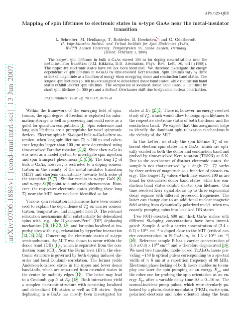
a r X i v :0706.1884v 1 [c o n d -m a t .m t r l -s c i ] 13 J u n 2007APS/123-QEDMapping of spin lifetimes to electronic states in n -type GaAs near the metal-insulatortransitionL.Schreiber,M.Heidkamp,T.Rohleder,B.Beschoten,∗and G.G¨u ntherodtII.Physikalisches Institut,and Virtual Institute for Spin Electronics (ViSel),RWTH Aachen University,Templergraben 55,52056Aachen,Germany(Dated:February 1,2008)The longest spin lifetimes in bulk n -GaAs exceed 100ns for doping concentrations near the metal-insulator transition (J.M.Kikkawa,D.D.Awschalom,Phys.Rev.Lett.80,4313(1998)).The respective electronic states have yet not been identiﬁed.We therefore investigate the energy dependence of spin lifetimes in n -GaAs by time-resolved Kerr rotation.Spin lifetimes vary by three orders of magnitude as a function of energy when occupying donor and conduction band states.The longest spin lifetimes (>100ns)are assigned to delocalized donor band states,while conduction band states exhibit shorter spin lifetimes.The occupation of localized donor band states is identiﬁed by short spin lifetimes (∼300ps)and a distinct Overhauser shift due to dynamic nuclear polarization.PACS numbers:78.47.+p,78.55.Cr,85.75.-dWithin the framework of the emerging ﬁeld of spin-tronics,the spin degree of freedom is exploited for infor-mation storage as well as processing and could serve as a qubit for quantum computation [1].Spin coherence and long spin lifetimes are a prerequisite for novel spintronic devices.Electron spins in Si-doped bulk n -GaAs drew at-tention,when long spin lifetimes T ∗2>100ns and coher-ence lengths larger than 100µm were determined using time-resolved Faraday rotation [2,3].Since then n -GaAs was used as a model system to investigate spin injectionand spin transport phenomena [4,5,6].The long T ∗2of bulk n -GaAs,however,is restricted to a doping concen-tration in the vicinity of the metal-insulator transition (MIT)and shortens dramatically towards both sides of the transition [2,7].Similar results in n -type GaN [8],and n -type Si [9]point to a universal phenomenon.How-ever,the respective electronic states yielding these long T ∗2near the MIT have not been identiﬁed so far.Various spin relaxation mechanisms have been consid-ered to explain the dependence of T ∗2on carrier concen-tration,temperature,and magnetic ﬁeld B .The relevant relaxation mechanisms diﬀer substantially for delocalized spins with,e.g.,the D’yakonov-Perel’(DP)dephasing mechanism [10,11,12,13],and for spins localized at im-purity sites with,e.g.,relaxation by hyperﬁne interaction [13,14,15].Concerning the electronic states of n -type semiconductors,the MIT was shown to occur within the donor band (DB)[16],which is separated from the con-duction band (CB).Near the Fermi level (E F ),the elec-tronic structure is governed by both doping induced dis-order and local Coulomb correlation.The former yields Anderson-localized states in the upper and lower donor band-tails,which are separated from extended states in the center by mobility edges [17].The latter may lead to a Coulomb gap U at E F [18].Both interactions yield a complex electronic structure with coexisting localized and delocalized DB states as well as CB states.Spin dephasing in n -GaAs has mostly been investigated forstates at E F [2,3].There is,however,no energy-resolvedstudy of T ∗2,which would allow to assign spin lifetimes to the respective electronic states of both the donor and the conduction band.We expect that this assignment helps to identify the dominant spin relaxation mechanisms in the vicinity of the MIT.In this Letter,we study the spin lifetime T ∗2of co-herent electron spin states in n -GaAs,which are opti-cally excited in both the donor and conduction band and probed by time-resolved Kerr rotation (TRKR)at 6K.Due to the coexistence of distinct electronic states,thesample is not characterized by a single T ∗2:T ∗2varies by three orders of magnitude as a function of photon en-ergy.The longest T ∗2values which may exceed 100ns are found for delocalized donor band states,while free con-duction band states exhibit shorter spin lifetimes.Our time-resolved Kerr signal shows up to three exponential decay regimes with diﬀerent precession frequencies.The latter can change due to an additional nuclear magnetic ﬁeld arising from dynamically polarized nuclei,when res-onantly pumping spins into localized DB states.Two (001)-oriented,500µm thick GaAs wafers with diﬀerent Si-doping concentrations have been investi-gated:Sample A with a carrier concentration of (2.4±0.2)×1016cm −3is doped close to the MIT (critical car-rier concentration in Si:GaAs n c ∼=1.5×1016cm −3)[16].Reference sample B has a carrier concentration of (1.5±0.4)×1018cm −3and is therefore degenerated [18].We used two tuneable,mode-locked Ti:Al 2O 3lasers pro-viding ∼150fs optical pulses corresponding to a spectral width of ≈6nm at a repetition frequency of 80MHz.Electronic phase-locking of both lasers enables us to em-ploy one laser for spin pumping at an energy E pu and the other one for probing the spin orientation at an en-ergy E pr after a variable delay time ∆t =0...16ns.The normal-incident pump pulses,which were circularly po-larized by a photo-elastic modulator (PEM),excite spin-polarized electrons and holes oriented along the beam2∆t (ps)θ∆t (ps)∆t (ps)sample Bsample A2.00-0.8θK (arb. units)7.60-5.3θK (arb. units)FIG.1:(Color)Time-resolved Kerr rotation for photon en-ergies E =E pu =E pr at 6K with (a)θK (∆t )for sample A at B =1T;the red line shows the shift of the beating node;(b)θK (∆t,E )for sample A at B =1T;(c)θK (∆t,E )for the degenerate sample B at B =6T.Arrows mark the respective energies,above which the transmission drops below 5%.direction in the strain-free mounted samples with an av-erage power P =50W/cm 2.The projection of the pump induced spin magnetization onto the surface nor-mal of the sample is determined with linearly polarized laser pulses by Faraday rotation θF in transmission and by Kerr rotation θK in reﬂection.Transverse magnetic ﬁelds B are applied in the plane of the sample.In Figure 1(a),we plot θK (∆t )of sample A measured for various photon energies E =E pu =E pr at B =1T and at T =6K.Obviously,the spins precess at all energies E ,but the damping of the oscillations andthus T ∗2is E -dependent:for E below the CB edge T ∗2is long,whereas for the highest E ,at which CB states arepumped,T ∗2is much reduced.Strikingly,a node in the oscillation envelope (red line in Fig.1(a))near the band edge indicates that the spins precess with at least two Larmor frequencies ω(i ).Therefore,θK (∆t )is described by n decay componentsθK (∆t )=n iA (i )exp−∆t3 constant and exhibits|g∗|=|g0|=0.43.Near the CBedge(green),B-independent values of T∗2∼100...300psare determined,which distinguish themselves by a rapiddecrease ofω(E).At the beginning of the third region(blue),T∗2sets-in at∼6ns and decreases with increasingE.The correspondingωdecreases slightly and saturatesat high E.The overlap in energy of the second and thirdregion,which occurs due to the spectral width of thelaser pulses,generates the node in the oscillation enve-lope shown in Figure1[19].For the degenerate sample B,T∗(i) 2(E)can beﬁtted by one component i.As expected[2,7],T∗2is over-all shorter compared to sample A and T∗2increases with the increase of B,which is typical for the DP dephasing mechanism[10].In the following,we assign the T∗(i)2of the spins ob-served in the three energy ranges to carriers occupying diﬀerent electronic states.Since hole spins relax quickly 10ps in GaAs and excitons are broken up at high magneticﬁelds B 1T[20],we consider single elec-tron states.Since the carrier concentration of sample A is slightly above n c,E F lies within the delocalized DB states as sketched in Figure3.Thus delocalized DB states are pumped at lowest E,which exhibit the longest T∗2(red component in Fig.2).However,to our knowl-edge there is no relaxation mechanism of spins,which accounts for their distinct B-dependence.We assign the second energy range(green),which is missing for the degenerate sample B,to Anderson localized electronic states at the DB tail.Their distinct E-dependence of ωand T∗2can be linked to the decrease of localization length upon approaching the DB tail.The localization of electrons yields spin relaxation due to hyperﬁne inter-action with the nuclei[14,15].This gives rise to dynamic nuclear polarization and a nuclearﬁeld,which altersω(Overhauser shift)[21].However,from Ref.[14]long T∗2∼300ns are expected for localized electron spins, although we could not reproduce this result with insu-lating n-GaAs samples using TRKR.In Ref.[15],an additional short T∗2∼100ps component is predicted, when both localized and delocalized spins are pumped. This is assigned to their cross-relaxation rate.Whereas this might explain our short T∗2,it does not account for the distinctω(E)dependence.In the third energy regime (blue),electrons are pumped in the CB.The decrease of ωobserved for both samples is due to g∗:The absorption of the pump pulse lifts the local chemical potential,thus reducing the absolute value of the energetically averaged g∗factor according to its dispersion in the CB[20].The apparent decrease of T∗2(E)might be explained by car-rier cooling and interband relaxation.Due to both,the carriers relax below the probed energy.This notion can be conﬁrmed by sweeping E pu with E pr heldﬁxed at the bottom of the CB.The corre-spondingﬁts of T∗(i)2(E pu)andω(i)(E pu)of sample Aat B=1T are shown in Figure3(a)and(b).Indeed,pr23452345E (eV)E (eV)T(i)2*(ps)T(i)2*(ps)ω(i)/ω0FIG.3:(Color)Upper left:sketch of density of DB and CBstates.Fitted spin lifetimes T∗(i)2and Larmor frequenciesω(i) as a function of pump laser energy E pu at magneticﬁelds B for MIT sample A(full symbols)for diﬀerent probe energies E pr is marked with vertical grey lines.For comparison data from Fig.2with E pu=E pr are also plotted(open symbols).this method allows to correct T∗2for energy relaxation, since T∗2(E pu)(blue full symbols)decreases only slightly compared to Figure2.However,there is an additionalshort T∗(i)2(E pu)(green full symbols),which results from probing localized spins at the DB tail because of the spec-tral width of the probe pulses.To clarify this point, E pr isﬁxed at an energy even lower than the band gap(Fig.3(c)-(e)).For this E pr,the longest T∗(i)2(E pu)(red) attributed to delocalized DB states is observed,which turned out to be nearly constant at B=0T.Note that the average pump power is held constant,but the excited carrier density changes by orders of magnitude in the ab-sorbing regime.This has a negligible eﬀect on the longest T∗2.More strikingly,additional components i become ob-servable,when E pu passes the localized and CB states. Thus,diﬀerent electronic states become occupied either due to direct optical excitation or carrier relaxation as sketched in Figure3(upper left).From the onset of the θF signal(not shown),we deduce that the delocalized DB states are occupied within∆t<10ps for all E pu. At B=1T(Fig.3(d))and E pu beyond the band edge,the two long T∗(i)2components(blue and red)generate nodes in the oscillation envelope(Fig.1(a))and can be separated by theirω(i)(Fig.3(e)).Forﬁtting,however, the longest T∗2(red)of delocalized DB had to beﬁxed with minor inﬂuence on the blue component.The lat-4∆t (ns)FIG.4:(Color)Faraday rotationθF(∆t)of sample A for left(σ−)and right(σ+)circularly polarized pump pulses(red ar-rows)at B=1T,E pu=1.514eV and E pr=1.494eV.Inset:ﬁtted normalized Larmor frequenciesω(i)and correspondinglateral nuclear magneticﬁelds BN for both polarizations as afunction of the average pump power.ter can be clearly assigned to CB states by comparing it to T∗2(E pu)and g∗(E pu)of Figure3(a)and(b).The existence of three components i and their onset whensweeping E pu conﬁrms our assignment of T∗(i)2(E)to thethree types of electronic states.Since an optically pumped spin imbalance of localized electrons leads to pronounced dynamic nuclear polariza-tion(DNP)[21],weﬁnally check our assignment of elec-tronic states to T∗2by identifying DNP.When resonantly exciting localized spins at,e.g.,E pu=1.514eV,then DNP is optically observed by the Overhauser shift.This shift results in a change ofωdue to the presence of a lateral nuclear magneticﬁeld B N adding up to B.Since spins exhibiting long T∗2are most sensitive to this shift, we chose the same E pr as in Figure3(c)-(e).In order to generate a well-deﬁned longitudinally pumped spin com-ponent and thus to control the direction of B N with re-spect to B,we replaced the PEM by a quarter-waveplate and rotated sample A as sketched in Figure4[22].In this geometry,θF(∆t)exhibits nodes in the oscillation envelope at long∆t,proving the presence of two longT∗(i) 2components with diﬀerentω(i).The dependence ofωon the type of circularly polarizationσ±of the pump pulses,is clariﬁed by theﬁttedω(i)in the inset of Fig-ure4.The sign and magnitude of B N is determined by σ±and the pump power,respectively.B N saturates for σ+at-90mT,when|g∗|=0.43is assumed to be con-stant.However,the blue component,which is likely due to spins in the CB(cp.to Fig.3(e)),is more sensitive to B N than the spins attributed to delocalized DB states (red).However,this point needs further investigation. Since DNP is not observable when E pu is reduced below 1.5eV,our assignment of localized states is conﬁrmed. The pronouncedω(loc)(E)dependence of the localized spins(green)(see Fig.2left)compared to theωvari-ation(blue)in the inset of Figure4suggests that the ω(loc)(E)is indeed inﬂuenced by increasing localization and thus responsible for a rise of B N at the DB tail[23]. In summary,we have studied the energy dependence of spin lifetimes in n-type GaAs for electron doping near the metal-insulator transition.Distinct spin lifetimes have been assigned to both donor and conduction band states. Spin states at the Fermi level are delocalized donor band states with the longest spin lifetime,which may exceed 100ns.The strong decrease of spin lifetimes in the con-duction band is related to energy relaxation of hot elec-trons.Localized donor band states exhibit the shortest spin lifetimes of∼300ps.Resonant optical pumping of these localized states yields strong dynamic nuclear po-larization.This work was supported by BMBF and by HGF.∗Electronic address:beschoten@physik.rwth-aachen.de [1]D.D.Awschalom and M.E.Flatte,Nature Phys.3,153(2007).[2]J.M.Kikkawa and D.D.Awschalom,Phys.Rev.Lett.80,4313(1998).[3]J.M.Kikkawa and D.D.Awschalom,Nature397,139(1999).[4]Y.Kato et al.,Science306,1910(2004).[5]S.A.Crooker et al.,Science309,2191(2005).[6]X.Lou et al.,Nature Phys.3,197(2007).[7]R.I.Dzhioev et al.,Phys.Rev.B66,245204(2002).[8]B.Beschoten et al.,Phys.Rev.B63,121202R(2001).[9]V.Zariﬁs and T.G.Castner,Phys.Rev.B36,6198(1987).[10]J.Fabian and S.D.Sarma,J.Vac.Sci.Technol.B17,1708(1999).[11]P.H.Song and K.W.Kim,Phys.Rev.B66,035207(2002).[12]Z.G.Yu et al.,Phys.Rev.B71,245312(2005).[13]B.I.Shklovskii,Phys.Rev.B73,193201(2006).[14]R.I.Dzhioev et al.,JETP Lett.74,200(2001).[15]W.O.Putikka and R.Joynt,Phys.Rev.B70,113201(2004).[16]D.Romero et al.,Phys.Rev.B42,3179(1990).[17]P.Anderson,Phys.Rev.189,1492(1958).[18]A.Efros and M.Pollak,eds.,Electron-Electron Interac-tion in Disordered Systems(North-Holland,Amsterdam, 1984).[19]The third region sets in at even lower energy E≈1.514eV,where T∗2cannot be determined exactly dueto the beating.[20]M.Oestreich et al.,Phys.Rev.B53,7911(1996).[21]D.Paget et al.,Phys.Rev.B15,5780(1977).[22]G.Salis et al.,Phys.Rev.B64,195304(2001).[23]Even with the PEM,ωchanges whithin∼1min afterswitching on the pump.We attribute this to an Over-hauser shift.。

Ising spin glass under continuous-distribution random magnetic fields Tricritical points an

a r X i v :0804.1342v 1 [c o n d -m a t .s t a t -m e c h ] 8 A p r 2008Ising Spin Glass Under Continuous-Distribution Random Magnetic Fields:Tricritical Points and Instability LinesNuno Crokidakis ∗and Fernando D.Nobre †Centro Brasileiro de Pesquisas F´ısicasRua Xavier Sigaud 15022290-180Rio de Janeiro -RJ Brazil(Dated:April 8,2008)The eﬀects of random magnetic ﬁelds are considered in an Ising spin-glass model deﬁned in the limit of inﬁnite-range interactions.The probability distribution for the random magnetic ﬁelds is a double Gaussian,which consists of two Gaussian distributions centered respectively,at +H 0and −H 0,presenting the same width σ.It is argued that such a distribution is more appropriate for a theoretical description of real systems than its simpler particular two well-known limits,namely the single Gaussian distribution (σ≫H 0),and the bimodal one (σ=0).The model is investigated by means of the replica method,and phase diagrams are obtained within the replica-symmetric solution.Critical frontiers exhibiting tricritical points occur for diﬀerent values of σ,with the possibility of two tricritical points along the same critical frontier.To our knowledge,it is the ﬁrst time that such a behavior is veriﬁed for a spin-glass model in the presence of a continuous-distribution random ﬁeld,which represents a typical situation of a real system.The stability of the replica-symmetric solution is analyzed,and the usual Almeida-Thouless instability is veriﬁed for low temperatures.It is veriﬁed that,the higher-temperature tricritical point always appears in the region of stability of the replica-symmetric solution;a condition involving the parameters H 0and σ,for the occurrence of this tricritical point only,is obtained analytically.Some of our results are discussed in view of experimental measurements available in the literature.Keywords:Spin Glasses,Random-Field Systems,Replica Method,Almeida-Thouless Instability.PACS numbers:05.50+q,64.60.-i,75.10.Nr,75.50.LkI.INTRODUCTIONSpin-glass systems[1,2,3,4,5]continue to challenge many researchers in the area of magnetism.¿From the theoretical point of view,its simplest version deﬁned in terms of Ising spin variables,the so-called Ising spin glass(ISG),represents one of the most fasci-nating problems in the physics of disordered magnets.The ISG mean-ﬁeld solution,based on the inﬁnite-range-interaction model,as proposed by Sherrington-Kirkpatrick(SK)[6], presents a quite nontrivial behavior.The correct low-temperature solution of the SK model is deﬁned in terms of a continuous order-parameter function[7](i.e.,an inﬁnite number of order parameters)associated with many low-energy states,a procedure which is usually denominated as replica-symmetry breaking(RSB).Furthermore,a transition in the presence of an external magneticﬁeld,known as the Almeida-Thouless(AT)line[8], is found in the solution of the SK model:such a line separates a low-temperature region, characterized by RSB,from a high-temperature one,where a simple one-parameter solu-tion,denominated as replica-symmetric(RS)solution,is stable.The validity of the results of the SK model for the description of more realistic systems,characterized by short-range-interactions,represents a very polemic question[5].Recent numerical simulations claim the absence of an AT line in the three-dimensional short-range ISG[9],as well as along the non-mean-ﬁeld region of a one-dimensional ISG characterized by long-range interactions [10].However,these results,obtained with rather small lattice-size simulations,do not rule out the possibility of a crossover to a diﬀerent scenario at much larger lattice sizes, or also for smallerﬁelds(and/or temperatures).One candidate for alternative theory to the SK model is the droplet model[11],based on domain-wall renormalization-group arguments for spin glasses[12,13].According to the droplet model,the low-temperature phase of anyﬁnite-dimensional∗E-mail address:nuno@cbpf.br†Corresponding author:E-mail address:fdnobre@cbpf.bra single thermodynamic state(together,of course,with its corresponding time-reversed counterpart),i.e.,essentially a RS-type of solution.Many important features of the ISG still deserve an appropriate understanding within the droplet-model scenario,and in par-ticular,the validity of this model becomes questionable for increasing dimensionalities, where one expects the existence of aﬁnite upper critical dimension,above which the mean-ﬁeld picture should prevail.Some diluted antiferromagnets,like Fe x Zn1−x F2,Fe x Mg1−x Cl2and Mn x Zn1−x F2,have been the object of extensive experimental research,due to their intriguing properties [14].These systems are able to exhibit,within certain concentration ranges,random-ﬁeld,spin-glass or both behaviors,and in particular,the compounds Fe x Zn1−x F2and Fe x Mg1−x Cl2are characterized by large crystal-ﬁeld anisotropies,in such a way that they may be reasonably well-described in terms of Ising variables.Therefore,they are usually considered as good physical realizations of the random-ﬁeld Ising model(RFIM),or also of an ISG.For the Fe x Zn1−x F2,one gets a RFIM-like behavior for x>0.42,an ISG for x∼0.25,whereas for intermediate concentrations(0.25<x<0.42)one may observe both behaviors depending on the magnitude of the applied external magneticﬁeld[RFIM (ISG)for small(large)magneticﬁelds],with a crossover between them[15,16,17].In what concerns Fe x Mg1−x Cl2,one gets an ISG-like behavior for x<0.55,whereas for0.7< x<1.0one has a typical RFIM with aﬁrst-order transition turning into a continuous one due to a change in the randomﬁelds[14,18,19].Even though a lot of experimental data is available for these systems,they still deserve an appropriate understanding,with only a few theoretical models proposed for that purpose[20,21,22,23,24,25,26,27]. Within the numerical-simulation technique,one has tried to take into account the basic microscopic ingredients of such systems[20,21,22,23],whereas at the mean-ﬁeld level, a joint study of both ISG and RFIM models has been shown to be a very promising approach[24,25,26,27].In the present work we investigate the eﬀects of random magneticﬁelds,following a continuous probability distribution,in an ISG model.The model is considered in the limit of inﬁnite-range interactions,and the probability distribution for the random mag-neticﬁelds is a double Gaussian,which consists of a sum of two independent Gaussian distributions.Such a distribution interpolates between the bimodal and the simple Gaus-sian distributions,which are known to present distinct low-temperature critical behavior, within the mean-ﬁeld limit[24,25,26,27].It is argued that this distribution is more appropriate for a theoretical description of diluted antiferromagnets than the bimodal and Gaussian distributions.In particular,for given ranges of parameters,this distribu-tion presents two peaks,and satisﬁes the requirement of eﬀective randomﬁelds varying in both sign and magnitude,which comes out naturally in the identiﬁcation of the RFIM with diluted antiferromagnets in the presence of a uniformﬁeld[28,29];this condition is not fulﬁlled by simple discrete probability distributions,e.g.,the bimodal one,which is certainly very convenient from the theoretical point of view.Recently,the use a double-Gaussian distribution in the RFIM[30]yielded interesting results,leading to a candidate model to describe the change of aﬁrst-order transition into a continuous one that occurs in Fe x Mg1−x Cl2[14,18,19].The use of this distribution in the study of the present model should be relevant for Fe x Mg1−x Cl2with concentrations x<0.55,where the ISG behavior shows up.In the next section we study the SK model in the presence of the above-mentioned random magneticﬁelds;a rich critical behavior is presented,and in par-ticular,oneﬁnds a critical frontier that may present one,or even two,tricritical points. The instabilities of the RS solution are also investigated,and AT lines presenting an in-ﬂection point,in concordance with those measured in some diluted antiferromagnets,are obtained.Finally,in section4we present our conclusions.II.THE ISING SPIN GLASS IN THE PRESENCE OF A RANDOM-FIELDThe inﬁnite-range-interaction Ising spin-glass model,in the presence of an external random magneticﬁeld,may be deﬁned in terms of the HamiltonianH=− (i,j)J ij S i S j− i H i S i,(1) where the sum (i,j)applies to all distinct pairs of spins S i=±1(i=1,2,...,N).The interactions{J ij}and theﬁelds{H i}follow independent probability distributions,FIG.1:The probability distribution of Eq.(3)(the randomﬁelds are scaled in units ofσ)for typical values of the ratio H0/σ:(a)(H0/σ)=1/3,1,5/2;(b)(H0/σ)=10.P(J ij)= N2J2 J ij−J0+exp −(H i+H0)22 12σ2[F({J ij,H i})]J,H= (i,j)[dJ ij P(J ij)] i[dH i P(H i)]F({J ij,H i}).(4) Now,one can make use of the replica method[1,2,3,4]in order to obtain the free energy per spin,−βf=lim N→∞1Nn([Z n]J,H−1),(5)where Z n represents the partition function of the replicated system andβ=1/(kT). Standart calculations lead toβf=−(βJ)22+limn→012 α(mα)2+(βJ)22ln Trαexp(H+eﬀ)−12<Sα>++12<Sαβ>++1where <>±indicate thermal averages with respect to the “eﬀective Hamiltonians”H ±effin Eq.(8).Assuming the RS ansatz [1,2,3,4],i.e.,m α=m (∀α)and q αβ=q [∀(αβ)],Eqs.(6)–(10)yieldβf =−(βJ )22m 2−1√212π ∞∞dze −z 2/2ln(2cosh ξ−),(11)m =1√212π +∞−∞dze −z 2/2tanh ξ−,(12)q =1√212π +∞−∞dze −z 2/2tanh 2ξ−,(13)whereξ±=β{J 0m +JGz ±H 0},(14)G = q + σJ 2=1√212π +∞−∞dze −z 2/2sech 4ξ−.(16)Let us now present the phase diagrams of this model.Since the random ﬁeld induces the parameter q ,there is no spontaneous spin-glass order,like the one found in the SK model.However,there is a phase transition related to the magnetization m ,in such a waythat two phases are possible within the RS solution,namely,the Ferromagnetic (m =0,q =0)and the Independent (m =0,q =0)ones.The critical frontier separating these two phases is obtained by solving the equilibrium conditions,Eqs.(12)and (13),whereasinthecase of ﬁrst-order phase transitions,the free energy per spin,Eq.(11),will be analyzed.Expanding the magnetization [Eq.(12)]in power series,m =A 1(q )m +A 3(q )m 3+A 5(q )m 5+O (m 7),(17)whereA 1(q )=βJ 0{1−ρ1(q )},(18)A 3(q )=−(βJ 0)315{2−17ρ1(q )+30ρ2(q )−15ρ3(q )},(20)andρk (q )=12π +∞−∞dze −z 2/2tanh 2k βJGz +H 01−(βJ )2Γm 2+O (m 4),(22)with Γ=1−4ρ1(q 0)+3ρ2(q 0),(23)where q 0corresponds to the solution of Eq.(13)for m =0.Substituting Eq.(22)in the expansion of Eq.(17),one obtains the m -independent coeﬃcients in the power expansionof the magnetization;in terms of the lowest-order coeﬃcients,one gets,m=A′1m+A′3m3+O(m5),(24)A′1=A1(q0),(25)A′3=−(βJ0)31−(βJ)2Γ Γ.(26)The associated critical frontier is determined through the standard procedure,taking into account the spin-glass order parameter[Eq.(13)],as well.For continuous transitions, A′1=1,with A′3<0,in such a way that one has to solve numerically the equation A′1=1,together with Eq.(13)considering m=0.If A′3>0,one may haveﬁrst-order phase transitions,characterized by a discontinuity in the magnetization;in this case,the critical frontier is found through a Maxwell construction,i.e.,by equating the free energies of the two phases,which should be solved numerically together with Eqs.(12)and(13) for each side of the critical line.When both types of phase transitions are present,the continuous andﬁrst-order critical frontiers meet at a tricritical point that deﬁnes the limit of validity of the series expansion.The location of such a point is determined by solving numerically equations A′1=1,A′3=0,and Eq.(13)with m=0[provided that the coeﬃcient of the next-order term in the expansion of Eq.(24)is negative,i.e.,A′5<0].Considering the above-mentioned phases,the AT instability of Eq.(16)splits each of them in two phases,in such a way that the phase diagram of this model may present four phases,that are usually classiﬁed as[24,25,26]:(i)Paramagnetic(P)(m=0;stability of the RS solution);(ii)Spin-Glass(SG)(m=0;instability of the RS solution);(iii) Ferromagnetic(F)(m=0;stability of the RS solution);(iv)Mixed Ferromagnetic(F′) (m=0;instability of the RS solution).Even though in most cases the AT line is computed numerically,for large values of J0[i.e.,J0>>J and J0>>H0]and low temperatures,one gets the following analytic asymptotic behavior,kT312π12J2G2 +exp−(J0−H0)2FIG.2:Phase diagrams of the inﬁnite-range-interaction ISG in the presence of a double-Gaussian randomﬁeld;the phases are labelled according to the deﬁnitions in the text.AT1and AT2 denote AT lines,and all variables are scaled in units of J.Two typical examples[(a)(σ/J)=0.2;(b)(σ/J)=0.6]are exhibited,for which there are single points(represented by black dots) characterized by A′1=1and A′3=0,deﬁning the corresponding threshold values H(1)0(σ).For the particular caseσ=0,i.e.,the bimodal probability distribution for theﬁelds [25],it was veriﬁed that the phase diagrams of the model change qualitatively and quan-titatively for incresing values of H0.Herein,we show that the phase diagrams of the present model change according to the parameters of the distribution of randomﬁelds [Eq.(3)],which may modify drastically the critical line separating the regions with m=0 and m=0,deﬁned by the coeﬃcients in Eq.(24).In particular,oneﬁnds numerically a threshold value,H(1)0(σ),for which this line presents a single point characterized by A′1=1and A′3=0;all other points of this line represent continuous phase transitions, characterized by A′1=1and A′3<0.Typical examples of this case are exhibited in Fig.2, for the dimensionless ratios(σ/J)=0.2and(σ/J)=0.6.As will be seen in the next ﬁgures,for values of H0/J slightly larger than H(1)0(σ)/J,this special point splits in two tricritical points,whereas for values of H0/J smaller than H(1)0(σ)/J,this critical frontier is completely continuous.Therefore,one may interpret the point for which H0=H(1)0(σ) as a collapse of two tricritical points.Such an unusual critical point is a characteristic of some inﬁnite-range-interaction spin-glasses in the presence of random magneticﬁelds [25,26],and to our knowledge,it has never been found in other magnetic models.¿From Fig.2,one notices that the threshold value H(1)0(σ)/J increases for increasing values ofσ/J,although the corresponding ratio H(1)0(σ)/σdecreases.Apart from that,this pecu-liar critical point always occurs very close to the onset of RSB;indeed,for(σ/J)=0.6, this point essentially coincides with the union of the two AT lines(AT1and AT2).At least for the range of ratiosσ/J investigated,this point never appeared below the AT lines,i.e.,in the region of RSB.Therefore,an analysis that takes into account RSB,will not modify the location of this point in these cases.In Fig.3we exhibit phase diagrams for aﬁxed value ofσ(σ=0.2J),and increasing values of H0.In Fig.3(a)we show the case(H0/J)=0.5,where one sees a phase diagram that looks like,at least qualitatively,the one of the SK model;even though the random-ﬁeld distribution[cf.Eq.(3)]is double-peaked(notice that(H0/σ)=2.5in this case),the eﬀects of such aﬁeld are not suﬃcient for a qualitative change in the phase diagram of the model.As we have shown above[see Fig.2(a)],qualitative changes only occur in the corresponding phase diagram for a ratio(H(1)0(σ)/σ)≈5,or higher.It is important to remark that a tricritical point occurs in the corresponding RFIM for any (H0/σ)≥1[30],in agreement with former general analyses[31,32,33].If one associates the tricritical points that occur in the present model as reminiscents of the one in the RFIM,one notices that such eﬀects appear attenuated in the present model due to the bond randomness,as predicted previously for short-range-interaction models[34,35].In Fig.3(b)we present the phase diagram for(H0/J)=0.993;in this case,one observes two ﬁnite-temperature tricritical points along the critical frontier that separates the regions with m=0and m=0.The higher-temperature point is located in the region where the RS approximation is stable,and so,it will not be aﬀected by RSB eﬀects;however,the lower-temperature tricritical point,found in the region of instability of the RS solution, may change under a RSB procedure.In Fig.3(c)we exhibit another interesting situation of the phase diagram of this model,for which the lower-temperature tricritical point goes down to zero temperature,deﬁning a second threshold value,H(2)0(σ).This threshold value was calculated analytically,through a zero-temperature approach that follows below,for arbitrary values ofσ/J.Above such a threshold,only the higher-temperature tricritical point(located in the region of stability of the RS solution)exists;this is shown in Fig.3(d), where one considers a typical situation with H0>H(2)0(σ).It is important to notice that in Fig.3(d)the two AT lines clearly do not meet at the critical frontier that separates theFIG.3:Phase diagrams of the inﬁnite-range-interaction ISG in the presence of a double-Gaussian randomﬁeld with(σ/J)=0.2and typical values of H0/J;the phases are labelled according to the deﬁnitions in the text.AT1and AT2denote AT lines,and all variables are scaled in units of J.By increasing the value of H0/J,the phase diagram changes both qualitatively and quantitatively and,particularly,the critical lines separating the regions with m=0and m=0are modiﬁed;along these critical frontiers,the full(dotted)lines represent continuous (ﬁrst-order)phase transitions and the black dots denote tricritical points;for the values of H0/J chosen,one has:(a)continuous phase transitions;(b)two tricritical points atﬁnite temperatures;(c)the lower tricritical point at zero temperature,deﬁning the corresponding threshold value H(2)0(σ);(d)a single tricritical point atﬁnite temperatures.regions with m=0and m=0;such an eﬀect is a consequence of the phase coexistence region,characteristic ofﬁrst-order phase transitions,and has already been observed in the SK model with a bimodal random-ﬁeld distribution[25].The line AT1is valid up to the right end limit of the phase coexistence region,whereas AT2remains valid up to theFIG.4:Phase diagrams of the inﬁnite-range-interaction ISG in the presence of a double-Gaussian randomﬁeld with(σ/J)=0.6and typical values of H0/J;the phases are labelled according to the deﬁnitions in the text.AT1and AT2denote AT lines,and all variables are scaled in units of J.Along the critical lines separating the regions with m=0and m=0,the full(dotted)lines represent continuous(ﬁrst-order)phase transitions and the black dots denote tricritical points; for the values of H0/J chosen,one has:(a)two tricritical points atﬁnite temperatures;(b)the lower tricritical point at zero temperature,deﬁning the corresponding threshold value H(2)0(σ).left end limit of such a region;as a consequence of this,the lines AT1and AT2do not meet at the corresponding Independent-Ferromagnetic critical frontier.Additional phase diagrams are shown in Fig.4,where we exhibit two typical cases for the random-ﬁeld width(σ/J)=0.6.In Fig.4(a)we show the equivalent of Fig.3(b), where two tricritical points appear atﬁnite temperatures;now one gets qualitatively a similar eﬀect,but with a random-ﬁeld distribution characterized by a smaller ratio H0/σ. From the quantitative point of view,the following changes occur,in the critical frontier Independent-Ferromagnetic,due to an increase inσ/J:(i)such a critical frontier moves to higher values of J0/J,leading to an enlargement of the Independent phase[corresponding to the region occupied by the P and SG phases of Fig.4(a)];(ii)the two tricritical points are shifted to lower temperatures.In Fig.4(b)we present the situation of a zero-temperature tricritical point,deﬁning the corresponding threshold value H(2)0(σ);once again,one gets a physical situation similar to the one exhibited in Fig.3(c),but with a much smaller ratio H0/σ.Qualitatively similar eﬀects may be also observed for other values ofσ,but with diﬀerent threshold values,H(1)0(σ)and H(2)0(σ).We have noticedFIG.5:Evolution of the threshold values H(1)0(σ)(lower curve)and H(2)0(σ)(upper curve)with the widthσ(all variables are scaled in units of J).Three distinct regions(I,II,and III)are shown,concerning the existence of tricritical points andﬁrst-order phase transitions along the Independent-Ferromagnetic critical frontier.The dashed straight line corresponds to H0=σ, above which one has a tricritical point in the corresponding RFIM[30].that such threshold values increase withσ/J,even though one requires less-pronounced double-peaked distributions[i.e.,smaller values for the ratios H0/σ]in such a way to get signiﬁcant changes in the standard SK model phase diagrams[as can be seen in Figs.2, 3(c),and4(b)].The evolution of the threshold values H(1)0(σ)and H(2)0(σ)with the dimensionless widthσ/J is exhibited in Fig.5.One notices three distinct regions in what concerns the existence of tricritical points andﬁrst-order phase transitions along the Independent-Ferromagnetic critical frontier.Throughout region I[deﬁned for H0>H(2)0(σ)]aﬁrst-order phase transition occurs atﬁnite temperatures and reaches the zero-temperature axis;a single tricritical point is found atﬁnite temperatures[a typical example is shown in Fig.3(d)].In region II[deﬁned for H(1)0(σ)<H0<H(2)0(σ)]oneﬁnds twoﬁnite-temperature tricritical points,with aﬁrst-order line between them[typical examples are exhibited in Figs.3(b)and4(a)].Along region III[H0<H(1)0(σ)]one has a completely continuous Independent-Ferromagnetic critical frontier[like in Fig.3(a)].The dashed straight line corresponds to H0=σ,which represents the threshold for the existence of a tricritical point in the corresponding RFIM[30].Hence,if one associates the occurrenceFIG.6:The zero-temperature phase diagram H0versus J0(in units of J)for two typical values of the dimensionless widthσ/J.The critical frontiers separating the phases SG and F′is continuous for small values of H0/J(full lines)and becomeﬁrst-order for higher values of H0/J(dotted lines);the black dots denote tricritical points.Although the two critical frontiers become very close near the tricritical points,they do not cross each other;the tricritical point located at a higher value of J0/J corresponds to the higher dimensionless widthσ/J.of tricritical points in the present model with those of the RFIM,one notices that such eﬀects are attenuated due to the bond randomness,in agreement with Refs.[34,35]; herein,the bond randomness introduces a spin-glass order parameter,in such a way that one needs stronger values of H0/J for these tricritical points to occur.Let us now consider the phase diagram of the model at zero temperature;in this case, the spin-glass order parameter is trivial(q=1),in such a way that the free energy and magnetization become,f=−J02 erfJ0m+H02 −erf J0m−H02−J2πG0 exp −(J0m+H0)22J2G20 ,(28)m=1JG0√2erf J0m−H02 ,(29)whereG0= 1+ σ2G0 J02J2G20 ,(32)a3=12G30 J0G20H02J2G20 ,(33)a5=12G50 J0G40H0G20 H02J2G20 .(34)For[H0/(JG0)]2<1[i.e.,a3<0],we have a continuous critical frontier given by a1=1,J0π2J2G20 .(35) This continuous critical frontier ends at a tricritical point(a3=0),1J 2=1⇒H0J=1+ σJ= 2 1+ σFIG.7:Typical phase diagrams of the inﬁnite-range-interaction ISG in the presence of a double-Gaussian randomﬁeld with(σ/J)=0.4are compared with those already known for some particular parisons of qualitatively similar phase diagrams are presented,essentially in what concerns the critical frontier that separates the regions with m=0and m=0.(a) Phase diagrams for the single Gaussian[(H0/J)=0.0and(σ/J)=0.4]and the double Gaussian [(H0/J)=0.8and(σ/J)=0.4]distributions for the randomﬁelds.(b)Phase diagrams for the bimodal[(H0/J)=0.9573]and the double Gaussian[(H0/J)=1.0447]distributions for the randomﬁelds.(c)Phase diagrams for the bimodal[(H0/J)=0.97]and the double Gaussian [(H0/J)=1.055]distributions for the randomﬁelds.(d)Phase diagrams for the bimodal [(H0/J)=1.0]and the double Gaussian[(H0/J)=1.077]distributions for the randomﬁelds. The phases are labelled according to the deﬁnitions in the text.AT1and AT2denote AT lines, and all variables are scaled in units of J.FIG.8:Instabilities of the replica-symmetric solution of the inﬁnite-range-interaction ISG(cases J0=0)in the presence of a double-Gaussian randomﬁeld,for two typical values of distribution widths:(a)(σ/J)=0.2;(b)(σ/J)=0.6.In each case the AT line separates a region of RS from the one characterized by RSB(all variables are scaled in units of J).Hence,Eqs.(36)and(37)yield the coordinates of the tricritical point at zero temperature. In addition to that,the result of Eq.(36)corresponds to the exact threshold value H(2)0(σ) (as exhibited in Fig.5).The above results are represented in the zero-temperature phase diagram shown in Fig.6,where oneﬁnds a single critical frontier separating the phases SG and F′.In order to illustrate that the present model is capable of reproducing qualitatively the phase diagrams of previous works,namely,the Ising spin glass in the presence of random ﬁelds following either a Gaussian[24],or a bimodal[25]probability distribution,in Fig.7 we compare typical results obtained for the Ising spin-glass model in the presence of a double Gaussian distribution characterized by(σ/J)=0.4with those already known for such particular cases.In these comparisons,we have chosen qualitatively similar phase diagrams,mainly taking into account the critical frontier that separates the regions with m=0and m=0.In Fig.7(a)we exhibit the phase diagram of the present model [(H0/J)=0.8]together with the one of an ISG in the presence of randomﬁelds described by a single Gaussian distribution;both phase diagrams are qualitatively similar to the one of the standard SK model.In Fig.7(b)we present phase diagrams for the bimodal and double Gaussian distributions,at their corresponding threshold values,H(1)0(σ).Typical situations for the cases of the bimodal and double Gaussian distributions,where two tricritical points appear along the critical frontier that separates the regions with m=0and m=0,are shown in Fig.7(c).Phase diagrams for the bimodal and double Gaussian distributions,at their corresponding threshold values,H(2)0(σ),are presented in Fig.7(d).Next,we analyze the AT instability for J0=0;in this case,Eq.(16)may be written askT√J ,(38)which corresponds to the same instability found in the case of a single-Gaussian random ﬁeld[24].In Fig.8we exhibit AT lines for two typical values of distribution widths;in each case the AT line separates a region of RS from the one characterized by RSB.One notices that the region associated with RSB gets reduced for increasing values ofσ;however,the most interesting aspect in these lines corresponds to an inﬂection point,which may be identiﬁed with the one that has been observed in the experimental equilibrium boundary of the compound Fe x Zn1−x F2[15,24].Up to now,this eﬀect was believed to be explained only through the ISG in the presence of a single-Gaussian randomﬁeld,for which the phase diagrams in the cases J0>0are much simpler,with all phase transitions being continuous, typically like those of the SK model.Herein,we have shown that an inﬂection point in the AT line may also occur in the present model,for which one has a wide variety of phase diagrams in the corresponding case J0>0,as exhibited above.Therefore,the present model would be appropriate for explaining a similar eﬀect that may be also observed experimentally in diluted antiferromagnets characterized byﬁrst-order phase transitions, like Fe x Mg1−x Cl2.III.CONCLUSIONSWe have studied an Ising spin-glass model,in the limit of inﬁnite-range interactions and in the presence of random magneticﬁelds distributed according to a double-Gaussian probability distribution.Such a distribution contains,as particular limits,both the single-Gaussian and bimodal probability distributions.By varying the parameters of this distri-。

黄色短杆菌中L-异亮氨酸同位素丰度及分布的分析方法研究

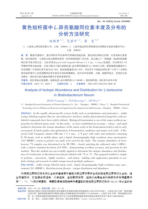
第43 卷第 3 期2024 年3 月Vol.43 No.3496~500分析测试学报FENXI CESHI XUEBAO（Journal of Instrumental Analysis）黄色短杆菌中L-异亮氨酸同位素丰度及分布的分析方法研究赵雅梦1，2，范若宁1，2，雷雯1，2*（1．上海化工研究院有限公司，上海　200062；2．上海市稳定同位素检测及应用研发专业技术服务平台，上海　200062）摘要：随着代谢组学、蛋白质组学等生命科学领域的迅猛发展，稳定同位素标记试剂，尤其是标记氨基酸，因无放射性、与非标记化合物理化性质一致等优势得到广泛应用。

该文建立了一种稳健、快速的氨基酸同位素丰度分析方法。

方法采用Hypersil Gold Vanquish（100 mm × 2.1 mm，1.9 μm）色谱柱，以水和含0.1%甲酸的甲醇为流动相，正离子模式下进行液相色谱-高分辨质谱联用（LC-HRMS）分析；测得细菌发酵液中L-异亮氨酸-15N的同位素丰度为98.58%，相对标准偏差为0.03%，可应用于不同稳定同位素（15N或13C）示踪的黄色短杆菌中L-异亮氨酸同位素丰度及分布的准确测定。

该方法具有简便、灵敏、稳健等优点，有望在合成生物学、同位素示踪代谢流等研究中发挥重要作用。

关键词：同位素标记氨基酸；液相色谱-高分辨质谱（LC-HRMS）；黄色短杆菌；同位素分布及丰度中图分类号：O657.72；O629.7文献标识码：A 文章编号：1004-4957（2024）03-0496-05Analysis of Isotope Abundance and Distribution for L-Isoleucinein Brebvibacterium flavumZHAO Ya-meng1，2，FAN Ruo-ning1，2，LEI Wen1，2*（1．Shanghai Research Institution of Chemical Industry Co. Ltd.，Shanghai　200062，China；2．Shanghai Professional Technology Service Platform on Detection and Application Development for Stable Isotope，Shanghai　200062，China）Abstract：In the rapidly advancing life science fields such as metabolomics and proteomics，stable isotope labeling reagents that are non-radioactive and have similar physiochemical properties with un⁃labeled compounds have been widely utilized. Biological fermentation is one of the major synthesis ap⁃proaches for labeled amino acids. In this study，we have established an accurate，robust，and rapid method to determine the isotope abundance of the amino acids in the fermentation broth to aid in early assessment of batch quality and optimization of fermentation conditions and amino acid yield. A Hy⁃persil Gold Vanquish column（100 mm × 2.1 mm，1.9 μm）with water and methanol containing 0.1%formic acid as mobile phase and a liquid chromatography-high resolution mass spectrometry（LC-HRMS） system in positive ion mode were used for the study. The isotopic abundance of L-iso⁃leucine-15N samples was determined to be 98.58%，closely matching the indicated value（>98%），with a relative standard deviation of 0.03%，demonstrating excellent accuracy and precision for the method. Then the method was successfully applied to determine the isotopic abundance and distribu⁃tion of L-isoleucine in Brevibacterium flavum labeled with 15N or 13C. The proposed method is simple to perform，convenient，highly sensitive，and robust，holding wide application potentials in syn⁃thetic biology and research in stable isotope traced metabolic pathways.Key words：stable isotope labeled amino acid；liquid chromatography-high resolution mass spec⁃trometry（LC-HRMS）；Brebvibacterium flavum；isotope distribution and abundance利用同位素标记技术将化合物中普通原子替换为同位素核素所合成的稳定同位素标记化合物，结合质谱技术，已在蛋白质组学、代谢组学、生物靶标发现、临床诊断等生命科学研究中发挥重要作用［1-4］。

PSEUDOSCALAR NEUTRAL HIGGS BOSON PRODUCTION IN POLARIZED γe COLLISIONS

2
Calculation of the Cross-Section γ e → eA0 process
The process γe → eA0 is described by two type of diagrams: box and triangle diagrams. From quite a number of diagrams, however, the main contributions arise from triangle ones with photon exchange. This is clear from the fact that, the photon pole diagrams give the 1
2 2 2 2 2 2 2 − NC Q2 t mt cot(β )C0 (t, mA0 , mt ) − NC Qb mb tan(β )C0 (t, mA0 , mb ) 2 2 2 2 − m2 τ tan(β )C0 (t, mA0 , mτ ) + 2mW m1 g11 C0 (t, mA0 , m1 ) 2 + 2mW m2 g22 C0 (t, m2 A0 , m2 ) ,
PSEUDOSCALAR NEUTRAL HIGGS BOSON PRODUCTION IN POLARIZED γ e COLLISIONS M. SAVCI
∗
Physics Department, Middle East Technical University 06531 Ankara, Turkey
Abstract We investigate the pseudoscalar neutral Higgs-boson A0 production in the po√ larized γe collisions with two diﬀerent center of mass energies s = 500 GeV and √ s = 1 T eV . The cross-section of the process γe → eA0 and the polarization asymmetry due the spin of the initial beams are calculated.

Cluso_Brochure_en_2015

FIRST ARTICLE INSPECTIONOriginally designed as a First ArticleInspection system, Cluso excels in thisspace. If human visual inspection isoccupying too much time during the linechangeover process, it’s very likely thatCluso will not only dramatically shortenthat time but improve the accuracy of thatprocess. While some existing first articletools help a little, Cluso is the only systemthat integrates all BOM, CAD & Visualimages in a single interface, with a step bystep process that ensures nothing ismissed. This fast, yet comprehensive,coverage ensures rapid line changeover.100% INSPECTION OF SMALL LOTSThe benefits of speed, efficiency &accuracy, so apparent with first articleinspection, encourage many users toharness the power & flexibility of the Clusosystem for 100% inspection of their smallbatch production. Unlike AOI systems,Cluso requires NO programming, & offersthe capability to inspect productaccurately, literally within minutes ofemerging from the production line.Moreover, inspection of through holedevices is as simple as SMT parts.END OF LINE or PRE-SHIPSome products (& some EMS customers!)demand a Pre-Ship visual inspection. Itmay be a full inspection or an audit but ifyou have to do it, then Cluso allows you tocut costs & improve accuracy while havingan audit trail.Can also do wire adds.NEW PRODUCT INTRO (NPI)It’s not a big leap from small lot inspectionto having a high value inspection tool inthe NPI area. The ability for inspection ofquick turn, small batch prototyping isexcellent & the resulting golden board isan ideal starting point for teaching an AOI!It really doesn’t matter the degree of automation you have in your facility, the questions that are most interesting are these: Are there people “looking” at PCBs on my floor? Is someone “checking” a PCB somewhere in my process?Do I have any product that I don’t trust enough to ship, without a final inspection?If this is happening, then perhaps Cluso can make it happen more effectively. Be it manual assembly, mixed technology PCBs or weaknesses in existing methods, including AOI, the Cluso Vision System may be the answer to some of these challenges.WHO NEEDS VISUALINSPECTION?DISTINCTLY DIFFERENT Cluso is, quite simply, a different way of looking at things.Especially PCBs!It is faster & more accurate than traditional techniques, yet it retains the human input, while making the task of inspection highly tolerable & successful forinspection personnel.THE CLUSO VISION SYSTEM AREAS OF APPLICATION AUDIT INSPECTIONThere are always concerns that an escapepast standard inspection tools will allow abatch of defective product to make itthrough. Cluso is an ideal tool for catchingthose challenging polarity marks orweeding out the errant reel errors.DOCUMENTATION CONTROLŸ Deskcheck BOM, CAD & Placement Data in advance of production date. Or really quickly if that’s today!Ÿ Evaluate discrepancies on screen, in real time INSPECTION PROCESSŸ Combines all Data & Images on screenŸ Can inspect all parts, one of each type, one part from each reel or selectively by user, e.g. All parts with polarityŸ Captures any discrepancies between rev levels Ÿ Equally effective for SMT & Through Hole parts QA RECORDS, ARCHIVING & TRACEABILITY Ÿ Stores CAD, BOM, images & QC report in a single PDF fileŸ Maintains exact product configuration for any build or rev levelŸ Verify component batch numbers from images on fileEASE OF USEŸ Ready to use in minutesŸ No programmingŸ No libraries to maintainŸ Single screen consolidation of all information required for the inspection processŸ Single screen comparison of product with sample Cluso is really the first company to acknowledge that visual inspection & human analysis is vital to the output of quality product.In accepting the human element,the challenge was to apply a level of technology that dramatically improved the ability of the inspector to produce a consistently good result. The goal was to eliminate the problems associated with concentration & issues of focus across a diverse data &image set, often too small for the eye to see. The Cluso Vision System captures & collates all the necessary information in a single frame of reference while presenting the work to be done in a simple, clear & concise manner to the operator, in a step by step format.A simple solution to a whole basket of challenges! Isn’t that the way it’s supposed to be?THE CLUSO VISION SYSTEMUNIQUE FEATURESWHAT MAKES CLUSO DIFFERENT?THE SCANNER MODULEŸProfessional grade scanner module for reliable, longterm PCB image capture capabilityŸEngineered optics for high resolution capture &50mm (2”) part height clearanceŸEnhance lighting system for clear capture of laseretched component markingsŸRugged housing & drawer assembly for durabilityon the shop floorTHE ENGINEŸQuad Core processor with 4GB RAM & large harddriveŸAll the power & storage you need to facilitate acomplete single station solution for all yourinspection needsTHE DATA CAPTURE KEYPADŸThe wireless keypad provides easy capture ofinspection data in a step by step mannerŸEasy P(ass) & F(ail) keys with user configurablekeys (F1 thru F4) for most common defectsŸTrigger input of comment fields with the Pc & Fckeys for added details on questionable Pass-FailconditionsŸFull Zoom, Cross Hair & Switching functionalityright on the keypadŸInput measured values via the Sm key with theintegration of a suitable multimeterTHE SOFTWAREŸWhy would we speak about software in theHardware section?We wouldn’t! Please call to arrange a 20 minuteonline presentation to see where the real magic ofCluso resides.In keeping with the Cluso ease of use philosophy, the operator interface is a very simple wireless keypad for data entry.With user defined failure mode keys, this effective data entry tool provides access to the vast majority of functionality required for the inspection process. This allows the inspector to focus on the job at hand. And that’s just exactly what we would like!THE CLUSO VISION SYSTEMTHE HARDWARECLUSO &SIMPLICITYEMS LARGE & SMALLŸ The EMS environment can be subjected to high line changeover with a punishing loss of line up time.Cluso can often recover 75% or more of this time.Ÿ Even smaller EMS houses can employ several inspectors for end of line or pre-ship inspection.Cluso can often reduce headcount by 50 to 75%.HIGH VOLUME, MOBILE PHONE & AUTOMOTIVE Ÿ New technology & high speed often go together.Cluso is a real asset for NPI & audit inspection in this go-fast environment where an error can literally spin into thousands of rejects. Ever missed an incorrect polarity mark on an automated line?MILITARY & MEDICALThe more critical the product, the more we fear trusting an automated system. Despite the fact that visual inspection has a terrible reputation, we still value, highly, what human intuition brings. Cluso keeps the intuition but it also adds in the accuracy.WHERE IT FITSŸ Anywhere that visual inspection is required,including through hole & wire adds.Ÿ Complimentary to, rather than a replacement for,AOI & other automated systems.Ÿ Where increased line utilization or reduced headcount is needed.Cluso is designed to save you time & resource, while improving quality. Who wouldn’t want some of that!This claim is not made lightly & it is supported by the simple fact that most of us spend a lot of time doing visual inspection. It doesn’t matter the cause: lack of trust in automated systems, customer mandate, critical product, been burned before, etc. Given that we have to do this, Cluso allows us to do it better & in far less time.The investment in Cluso falls far below that of even a limited capability desktop AOI machine.Yet the direct inspection time saved, & the consequential resource utilization because of that, allows for really fast payback. Outside of hard cost recovery, we can add the benefits of improvements in employee &customer satisfaction. Not bad!THE CLUSO VISION SYSTEMIN THE REAL WORLDIS CLUSO COSTEFFECTIVE?CLUSO BREAKS ALL THERULESThis image shows thecreativity of a Cluso ownerwho uses an image of the CADlayout drawing for the firstinspection of a new product.Without a golden sample, thedrawing substitutes as atemporary fix to improve theefficiency of getting to thatfirst golden sample. You mightalso use a scan of a bareboard, where referencedesignator markings wouldfacilitate the first pass.Towards the bottom left, notethe ability to offer images ofmulti-vendor parts againstany inspection step.SPECIFICATION Model A301 EH Max PCB Size (Scan Area)295mm x 420mm 11.6” x 16.5”Max Panel SizeApprox 400mm x 550mm Approx 15.7” x 21.6”Smallest Component Size01005Height Clearance50mm (<2”)Max Sample CapacityLimited by Disk Capacity Power Requirements110-240V 50/60Hz Weight - Scanner Module30 Kgs (66 lbs)Dimensions - Scanner Width x Depth x Height720mm x 500mm x 230mm28.5” x 19.5” x 9”CLUSO SPECIFICATIONSSCREENPRINTER PLACEMENT REFLOW AOIWAVESOLDERING POST WAVE INSPECTION PRE-SHIP OR FINALINSPECTIONBOM/CADDESKCHECKCLUSO INSPECTION OPPORTUNITY ZONES PRE-SHIP OR FINAL INSPECTIONTHROUGH HOLE OR MIXED TECHNOLOGY INSPECTIONFIRST ARTICLE OR 100% SMALL LOT INSPECTIONPRE-PRODUCTION BOM/CAD COMPARISON。

冷原子光谱法英语

冷原子光谱法英语Okay, here's a piece of writing on cold atom spectroscopy in an informal, conversational, and varied English style:Hey, you know what's fascinating? Cold atom spectroscopy! It's this crazy technique where you chill atoms down to near absolute zero and study their light emissions. It's like you're looking at the universe in a whole new way.Just imagine, you've got these tiny particles, frozen in place almost, and they're still putting out this beautiful light. It's kind of like looking at a fireworks display in a snow globe. The colors and patterns are incredible.The thing about cold atoms is that they're so slow-moving, it's easier to measure their properties. You can get really precise data on things like energy levels andtransitions. It's like having a super-high-resolution microscope for the quantum world.So, why do we bother with all this? Well, it turns out that cold atom spectroscopy has tons of applications. From building better sensors to understanding the fundamental laws of nature, it's a powerful tool. It's like having a key that unlocks secrets of the universe.And the coolest part? It's just so darn cool! I mean, chilling atoms to near absolute zero? That's crazy science fiction stuff, right?。

Meson Mixing in Pion Superfluid

2 metry and chiral symmetry. At ﬁnite isospin chemical potential, the isospin symmetry SUI (2) and chiral symmetry SUA (2) are explicitly broken to UI (1) and UA (1), respectively. Therefore, the chiral symmetry restoration at ﬁnite isospin chemical potential means only degeneracy of σ and π0 mesons, the charged π+ and π− behave still diﬀerently. Introducing the chiral and pion condensates ¯ = σu + σd , σ = ψψ ¯ , σu = u ¯u , σd = dd √ √ ¯ 5 τ+ ψ = 2 ψiγ ¯ 5 τ− ψ π = 2 ψiγ (2) √ with τ± = (τ1 ± iτ2 )/ 2 and taking all the condensates to be real, the quark propagator in mean ﬁeld approximation can be expressed as a matrix in the ﬂavor space S (p) = Suu (p) Sud (p) Sdu (p) Sdd (p) (3) d. The coupled set of gap equations (5) determines selfconsistently the three condensates. The isospin chemical potential dependence of the eﬀective quark mass Mq and pion condensate π is explicitly shown in [8]. The phase transition from the normal phase to the pion superﬂuid is of second order. In the NJL model, the meson modes are regarded as quantum ﬂuctuations above the mean ﬁeld. The two quark scattering via meson exchange can be eﬀectively expressed at quark level in terms of quark bubble summation in RPA[20]. The quark bubbles, namely the meson polarization functions are deﬁned as[21] Πmn (k ) = i

Decay widths and energy shifts of pi pi and pi K atoms

a r X i v :h e p -p h /0401048v 2 31 M a r 2004Decay widths and energy shifts of ππand πKatomsJ.SchweizerInstitute for Theoretical Physics,University of Bern,Sidlerstrasse 5,CH-3012Bern,SwitzerlandE-mail:schweizer@itp.unibe.ch1IntroductionNearly ﬁfty years ago,Deser et al.[1]derived the formulae for the decay width and strong energy shift of pionic hydrogen at leading order in isospin symme-try breaking.Similar relations also hold for π+π−[2]and π−K +atoms,which decay predominantly into 2π0and π0K 0,respectively.These Deser-type rela-tions allow to extract the scattering lengths from measurements of the decay width and the strong energy shift.The DIRAC collaboration [3]at CERN in-tends to measure the lifetime of pionium in its ground state at the 10%level,which will allow to extract the scattering length diﬀerence |a 00−a 20|at 5%accuracy.The experimental result can then be compared with theoretical pre-dictions for the S-wave scattering lengths [4–6]and with the results from other experiments [7].Particularly interesting is the fact that one may determine in this manner the nature of the SU(2)×SU(2)spontaneous chiral symmetry breaking experimentally [8].New experiments are proposed for CERN PS and J-PARC in Japan [9].In order to determine the scattering lengths from such experiments,the theoretical expressions for the decay width and the strong energy shift must be known to an accuracy that matches the experimentalprecision.For this reason,the ground state decay width of pionium has been evaluated at next-to-leading order[10–15]in the isospin symmetry breakingparameterδ,where both theﬁne-structure constantαand(m u−m d)2count as O(δ).The aim of the present article is to provide the corresponding for-mulae for the S-wave decay widths and strong energy shifts of pionium and theπ±K∓atom at next-to-leading order in isospin symmetry breaking.A detailed derivation of the results will be provided elsewhere[16].The strong energy shift of theπ±K∓atom is proportional to the sum of the isospin even and odd S-waveπK scattering lengths a+0+a−0.This sum[18–22]is sensitive to the combination of low-energy constants2L r6+L r8[23].The consequences of this observation for the SU(3)×SU(3)quark condensate[24]remain to be worked out.2Non-relativistic frameworkThe non-relativistic eﬀective Lagrangian framework has proven to be a very eﬃcient method to investigate bound state characteristics[12,15,25,26].The non-relativistic Lagrangian is exclusively determined by symmetries,which are rotational invariance,parity and time reversal.It provides a systematic expansion in powers of the isospin breaking parameterδ.What concerns the π−K+atom,we count bothαand m u−m d as orderδ.The diﬀerent power counting for theπ+π−andπ−K+atoms are due to the fact that in QCD,thechiral expansion of the pion mass diﬀerence∆π=M2π+−M2π0is of second orderin m u−m d,while the kaon mass diﬀerence∆K=M2K+−M2K0starts atﬁrst order in m u−m d.In the sector with one or two mesons,the non-relativistic πK Lagrangian is L NR=L1+L2.Theﬁrst term contains the one-pion and one-kaon sectors,L1=12Mh0+∆22M h++D4and δ4,respectively,L 2=C ′1π†−K †+π−K ++C 2π†−K †+π0K 0+h.c+C 3π†0K †0π0K 0+···(2)The ellipsis stands for higher order terms 1.We work in the center of masssystem and thus omit terms proportional to the total 3-momentum.The total and reduced masses readΣi =M πi +M K i ,µi =M πi M K i6r 2π++ r 2K +,(4)where r 2π+ and r 2K + denote the charge radii of the charged pion and kaon,respectively.The low energy constants C 1,...,C 3may be determined through matching the πK amplitude at threshold for various channels,see section 3.To evaluate the energy shift and decay width of the π−K +atom at next-to-leading order in isospin symmetry breaking,we make use of resolvents.For a detailed discussion of the technique,we refer to Ref.[15].Here,we simply list the results.We use dimensional regularization,to treat both ultraviolet and infrared singularities.Up to and including order δ9/2,the decay into π0K 0is the only decay channel contributing,and we get for the total S-wave decay widthΓn =α3µ3+4π2−αµ2+C 1ξn8M 3π0+M 3K 0n +ln2µ+n,Λ(µ)=µ2(d −3)11The basis of operators containing two space derivatives can be chosen such thatnone of them contributes to the energy shift and decay width at next-to-leading order in isospin symmetry breaking [16].withψ(n)=Γ′(n)/Γ(n)and the running scaleµ.At orderδ4,the total energy shift may be split into a strong part and an electromagnetic part,according to∆E n=∆E h n+∆E em n.(7) For the discussion of the electromagnetic energy shift,we refer to section4. The strong S-wave energy shift reads∆E h n=−α3µ3+2πC21ξn−µ20k202T lm;ikNR(q;p),(9)withωi(p)=(M2i+p2)1/2.The3-momentum p denotes the center of mass momentum of the incoming particles,q the one of the outgoing particles. The eﬀective Lagrangian in Eqs.(1)and(2),allows us to evaluate the non-relativisticπ−K+→π0K0andπ−K+→π−K+scattering amplitudes at threshold at orderδ.In the isospin symmetry limit,the eﬀective couplings C1,C2and C3areC1=2π2πµ+a+0,(10)where the S-wave scattering lengths2a+0=1/3(a1/20+2a3/20)and a−0= 1/3(a1/20−a3/20)are deﬁned in QCD,at m u=m d and Mπ.=Mπ+,M K.=M K+. By substituting these relations into the expression for the decay width(5) and the strong energy shift(8),one obtains the Deser-type formulae[1,2]. We demonstrate the matching at next-to-leading order inδby means of the π−K+→π−K+amplitude.In the presence of virtual photons,weﬁrst have to subtract the one-photon exchange diagram from the full amplitude,as dis-played in Fig.1.The coupling constant C1is determined by the truncated part¯T±;±NR,which contains an infrared singular Coulomb phaseθc as d→3,=+|p|µd−312[ln4π+Γ′(1)]+ln2|p||p|+B′2ln|p|4Mπ+M K+Re A±;±thr+O(p),(12) with B′1=C1απµ++o(δ),B′2=−C21αµ2+/π+o(δ)and12π 1−Λ(µ)−ln4µ2+2π2(Σ+−Σ0)+o(δ).(13)Here,the ultraviolet pole termΛ(µ)is removed by renormalizing the coupling C1.The renormalization of C1eliminates at the same time the ultraviolet divergence contained in the expression for the energy shift(8).The calcula-tion of the relativisticπ−K+→π−K+scattering amplitude was performed at O(p4,e2p2)in Refs.[20,21].Both the Coulomb phase and the logarithmic singularity in Eq.(12)are absent in the real part of the relativistic ampli-tude at this order of accuracy,theyﬁrst occur at order e2p4.The quantityRe A±;±thrdenotes the constant term occurring in the real part of the truncated relativistic threshold amplitude.The coupling constant C2may be determined analogously by matching the non-relativisticπ−K+→π0K0amplitude to the relativistic one at orderδ.4Results for theπ−K+atomThe result for the decay width and strong energy shift are valid at next-to-leading order in isospin symmetry breaking,and to all orders in the chiralexpansion.We get for the decay width at order δ9/2,in terms of the relativistic π−K +→π0K 0threshold amplitude,Γn =88√Σ+Re A 00;±thr +o (δ),(14)whereK n =M π+∆K +M K +∆πn+lnα2E nλE 2n ,M 2π0,M 2K 01/2,(16)with λ(x,y,z )=x 2+y 2+z 2−2xy −2xz −2yz ,is chosen such that the total ﬁnal state energy corresponds to E n =Σ+−α2µ+/(2n 2).The quantityRe A 00;±thr is calculated as follows.One evaluates the relativistic π−K +→π0K 0amplitude near threshold and removes the divergent Coulomb phase.The real part contains singularities ∼1/|p |and ∼ln |p |/µ+.The constant term in thisexpansion corresponds to Re A 00;±thr .The normalization is chosen such thatA =a −0+ǫ.(17)The isospin breaking corrections ǫhave been evaluated at O (p 4,e 2p 2)in Refs.[21,27].See also the comments in section 6.We now discuss the various energy shift contributions.According to Eq.(7),the energy shift at order δ4is split into an electromagnetic part ∆E emnand the strong part ∆E hn in Eq.(8).The electromagnetic energy shift contains both pure QED corrections as well as ﬁnite size eﬀects due to the charge radii of the pion and kaon,contained in λ.The pure electromagnetic corrections have been evaluated in Ref.[28]for arbitrary angular momentum l .We checked 3that the electromagnetic energy shift at order α4indeed amounts to∆E em nl=α4µ+Σ+32l +1+4α4µ3+λΣ+1n 4−33We thank A.Rusetsky for a very useful communication concerning technicalaspects of the calculation.Here,theﬁrst term is generated by the mass insertions,the second contains theﬁnite size eﬀects and the last stems from the one-photon exchange contri-bution.The strong S-wave energy shift reads at orderδ4,∆E h n=−2α3µ2+8πΣ+Re A±;±thr+o(δ),(19)withK′n=−2αµ+(a+0+a−0) ψ(n)−ψ(1)−1n +o(δ).(20) In the isospin limit,the normalized relativistic amplitudeA′=a+0+a−0+ǫ′,(21)reduces to the sum of the isospin even and odd scattering lengths.The cor-rectionsǫ′have been obtained at O(p4,e2p2)in Refs.[20,21].See also the comments in section6.The result for∆E h1in Eq.(19)agrees with the one obtained for the strong energy shift of the ground state in pionic hydrogen[26],if we replaceµ+with the reduced mass of theπ−p atom and Re A±;±thr with the constant term in the threshold expansion for the real part of the truncatedπ−p→π−p amplitude.What remains to be added are the vacuum polarization contributions[14,29], which are formally of higher order inα,however numerically not negligible. The vacuum polarization leads to an energy level shift∆E vac nl as well as to a change in the Coulomb wave function of theπ−K+atom at the origin δψK,n(0).For theﬁrst two energy levels,∆E vac nl[14,29]is given numerically in table2,section6.Formally of orderα2l+5,this contribution is enhanced due to its large coeﬃcient containing(µ+/m e)2l+2.The modiﬁed Coulomb wave function aﬀects both,the decay width and the strong energy shift,see section 6.As discussed in section6,the electromagnetic contributions(18)are known to a high precision.Further,the strong shift in the n P state is very much sup-pressed(orderα5).A future measurement of the energy splitting between the n S and n P states will therefore allow to extract the strong S-wave energy shift in Eq.(19),and to determine the combination a+0+a−0of theπK scattering lengths.The energy splitting between the2S and2P states is given by∆E2s−2p=∆E h2+∆E em20−∆E em21+∆E vac20−∆E vac21=−1.4±0.1eV.(22)The uncertainty displayed is the one in∆E h2only.For the numerical values of the various energy shift contributions,see table2in section6.5Results for pioniumThe decay rate and strong energy shift of pionium can be obtained from the formulae in Eqs.(5)and (8)through the following substitutions of the masses M K +→M π+,M K 0→M π0and the coupling constants C 1→c 1,C 2→√9n 3α3p ∗π,n A 2π(1+K π,n ),A π=a 00−a 20+ǫπ,K π,n =κ32a 00+a 2ψ(n )−ψ(1)−1n+o (δ),p ∗π,n=∆π−α2n 3A ′π1+K ′π,n,A ′π=132a 00+a 20ψ(n )−ψ(1)−1n+o (δ),(24)where A ′πis deﬁned analogously to the quantity A ′discussed in section 4.Theisospin symmetry breaking contributions ǫ′πhave been calculated at O (e 2p 2)in Refs.[31,32].For pionium the energy splitting between the 2S and 2P states reads∆E π,2s −2p =∆E h π,2+∆E em π,20−∆E em π,21+∆E vac π,20−∆E vacπ,21=−0.59±0.01eV .(25)Again the uncertainty displayed is the one in ∆E hπ,2only.The numerical values for the various energy shifts are listed in table 3,section 6.δ′h,1π+π−atom(6.2±1.2)·10−2(4.0±2.2)·10−2(1.5±2.2)·10−2 Table1Next-to-leading order corrections to the Deser-type formulae.6Numerical analysisFor the S-waveππscattering lengths,we use the chiral predictions a00=0.220±0.005and a20=−0.0444±0.0010[5,6].The correlation matrix for a00and a20 is given in Ref.[6].For the isospin symmetry breaking corrections to theππthreshold amplitudes(23)and(24),we useǫπ=(0.61±0.16)·10−2and ǫ′π=(0.37±0.08)·10−2as given in Ref.[15]and[32],respectively.For the πK scattering lengths,we use the values from the recent analysis of dataand Roy-Steiner equations[22],a+0=(0.045±0.012)M−1π+and a−0=(0.090±0.005)M−1π+.The correlation parameter for a+0and a−0is given in Ref.[22].The isospin breaking corrections to theπK threshold amplitudes(17)and (21)have been worked out in[20,21,27].Whereas the analytic expressions for ǫandǫ′obtained in[20,21,27]are not identical,the numerical values agree within the uncertainties quoted in[21].In the following,we use[21]ǫ=(0.1±0.1)·10−2M−1π+andǫ′=(0.1±0.3)·10−2M−1π+.For the charge radii of the pionand kaon,we take r2π+ =(0.452±0.013)fm2and r2K+=(0.363±0.072)fm2[33].We obtain for the decay width of the ground state,Γ1=8α3µ2+p∗1(a−0)2(1+δK,1),Γπ,1=2α3n3(a+0+a−0) 1+δ′K,n ,∆E hπ,n=−α3Mπ+π±K∓atom∆E vac[eV]τn[s]nl−0.095−9.0±1.1−0.019−1.1±0.1−0.006∆E emπ,nl[eV]∆E hπ,n[eV]n=1,l=0−0.942(2.9±0.1)·10−15 n=2,l=0−0.111n=2,l=1−0.004Table3Numerical values for the energy shift and the lifetime of theπ+π−atom. where2δψh,n(0)δvac h,n=7Summary and ConclusionsWe provided the formulae for the energy shifts and decay widths of theπ+π−andπ±K∓atoms at next-to-leading order in isospin symmetry breaking.To confront these predictions with data presents a challenge for future hadronic atom experiments.Should it turn out that these predictions are in conﬂict with experiment,one would have to revise our present understanding of the low-energy structure of QCD.AcknowledgmentsIt is a great pleasure to thank J.Gasser for many interesting discussions and suggestions.Further,I thank R.Kaiser,A.Rusetsky,H.Sazdjian and J.Schacher for useful discussions as well as for helpful comments on the manuscript.This work was supported in part by the Swiss National Sci-ence Foundation and by RTN,BBW-Contract N0.01.0357and EC-Contract HPRN–CT2002–00311(EURIDICE).References[1]S.Deser,M.L.Goldberger,K.Baumann and W.Thirring,Phys.Rev.96(1954)774;T.L.Trueman,Nucl.Phys.26(1961)57.[2]T.R.Palfrey and J.L.Uretsky,Phys.Rev.121(1961)1798;S.M.Bilenky,V.H.Nguyen,L.L.Nemenov and ebuchava,Yad.Fiz.10(1969)812.[3] B.Adeva et al.,CERN-SPSLC-95-1.[4]S.Weinberg,Phys.Rev.Lett.17(1966)616;J.Gasser and H.Leutwyler,Phys.Lett.B125(1983)321;J.Bijnens,G.Colangelo,G.Ecker,J.Gasser and M.E.Sainio,Phys.Lett.B374(1996)210[arXiv:hep-ph/9511397];J.Bijnens,G.Colangelo,G.Ecker,J.Gasser and M. E.Sainio,Nucl.Phys.B508(1997)263[Erratum-ibid.B517(1998)639][arXiv:hep-ph/9707291];J.Nieves and E.Ruiz Arriola,Eur.Phys.J.A8(2000)377[arXiv:hep-ph/9906437];G.Amoros,J.Bijnens and P.Talavera,Nucl.Phys.B585(2000)293[Erratum-ibid.B598(2001)665][arXiv:hep-ph/0003258].[5]G.Colangelo,J.Gasser and H.Leutwyler,Phys.Lett.B488(2000)261[arXiv:hep-ph/0007112].[6]G.Colangelo,J.Gasser and H.Leutwyler,Nucl.Phys.B603(2001)125[arXiv:hep-ph/0103088].[7]L.Rosselet et al.,Phys.Rev.D15(1977)574;C.D.Froggatt and J.L.Petersen,Nucl.Phys.B129,89(1977);M.M.Nagels et al.,Nucl.Phys.B147 (1979)189; A. A.Bolokhov,M.V.Polyakov and S.G.Sherman,Eur.Phys.J.A1(1998)317[arXiv:hep-ph/9707406]; D.Pocanic,arXiv:hep-ph/9809455;CHAOS Collaboration,J. nge et al.,Phys.Rev.Lett.80,1597(1998);J. nge et al.,Phys.Rev.C61(2000)025201;NA48Collaboration,R.Batley et al.,CERN-SPSC-2000-003;S.Pislak et al.[BNL-E865Collaboration],Phys.Rev.Lett.87(2001)221801[arXiv:hep-ex/0106071];S.Descotes-Genon,N.H.Fuchs,L.Girlanda and J.Stern,Eur.Phys.J.C24(2002)469[arXiv:hep-ph/0112088];S.Pislak et al.,Phys.Rev.D 67(2003)072004[arXiv:hep-ex/0301040];V.N.Maiorov and O.O.Patarakin, arXiv:hep-ph/0308162.[8]M.Knecht,B.Moussallam,J.Stern and N.H.Fuchs,Nucl.Phys.B457(1995)513[arXiv:hep-ph/9507319];M.Knecht,B.Moussallam,J.Stern and N.H.Fuchs,Nucl.Phys.B471(1996)445[arXiv:hep-ph/9512404];L.Girlanda, M.Knecht, B.Moussallam and J.Stern,Phys.Lett.B409(1997)461 [arXiv:hep-ph/9703448].[9] B.Adeva et al.,CERN-SPSC-2000-032;L.Afanasyev et al.,Lifetimemeasurement ofπ+π−andπ±K∓atoms to test low energy QCD(2002),letter of intent of the experiment at Japan Proton Accelerator Research Complex;available at http://dirac.web.cern.ch/DIRAC/future.html.[10]Z.K.Silagadze,JETP Lett.60(1994)689[arXiv:hep-ph/9411382];A.Gashi,G.Rasche,G.C.Oades and W.S.Woolcock,Nucl.Phys.A628(1998)101[arXiv:nucl-th/9704017];Z.K.Silagadze,arXiv:hep-ph/9803307;M.A.Ivanov, V.E.Lyubovitskij,E.Z.Lipartia and A.G.Rusetsky,Phys.Rev.D58 (1998)094024[arXiv:hep-ph/9805356];P.Minkowski,in:Proceedings of the International Workshop Hadronic Atoms and Positronium in the Standard Model,Dubna,26-31May1998,M.A.Ivanov at al.,Eds.,Dubna1998,p.74[arXiv:hep-ph/9808387];E.A.Kuraev,Phys.Atom.Nucl.61(1998)239;U.Jentschura,G.Soﬀ,V.Ivanov and S.G.Karshenboim,Phys.Lett.A241 (1998)351;H.W.Hammer and J.N.Ng,Eur.Phys.J.A6(1999)115 [arXiv:hep-ph/9902284].[11]H.Jallouli and H.Sazdjian,Phys.Rev.D58(1998)014011[Erratum-ibid.D58(1998)099901][arXiv:hep-ph/9706450];H.Sazdjian,Phys.Lett.B490(2000) 203[arXiv:hep-ph/0004226].[12]belle and K.Buckley,arXiv:hep-ph/9804201;X.Kong and F.Ravndal,Phys.Rev.D59(1999)014031;Phys.Rev.D61(2000)077506[arXiv:hep-ph/9905539]; B.R.Holstein,Phys.Rev.D60(1999)114030[arXiv:nucl-th/9901041];A.Gall,J.Gasser,V.E.Lyubovitskij and A.Rusetsky,Phys.Lett.B462(1999)335[arXiv:hep-ph/9905309];D.Eiras and J.Soto,Phys.Rev.D 61(2000)114027[arXiv:hep-ph/9905543];V.Antonelli,A.Gall,J.Gasser andA.Rusetsky,Annals Phys.286(2001)108[arXiv:hep-ph/0003118].[13]J.Gasser,V.E.Lyubovitskij and A.Rusetsky,Phys.Lett.B471(1999)244[arXiv:hep-ph/9910438].[14]D.Eiras and J.Soto,Phys.Lett.B491(2000)101[arXiv:hep-ph/0005066].[15]J.Gasser,V.E.Lyubovitskij,A.Rusetsky and A.Gall,Phys.Rev.D64(2001)016008[arXiv:hep-ph/0103157].[16]J.Schweizer,in preparation.The calculation of the same quantities in theframework of constrained Bethe-Salpeter equation is in progress[17].[17]H.Sazdjian,private communication.[18]V.Bernard,N.Kaiser and U.G.Meissner,Phys.Rev.D43(1991)2757.[19]A.Roessl,Nucl.Phys.B555(1999)507[arXiv:hep-ph/9904230].[20]A.Nehme,Eur.Phys.J.C23(2002)707[arXiv:hep-ph/0111212];B.Kubisand U.G.Meissner,Phys.Lett.B529(2002)69[arXiv:hep-ph/0112154]. [21]B.Kubis,Dissertation Bonn Univ.(2002).Berichte des ForschungszentrumsJ¨u lich,4007ISSN0944-2952.[22]P.Buettiker,S.Descotes-Genon and B.Moussallam,arXiv:hep-ph/0310283.[23]J.Gasser and H.Leutwyler,Nucl.Phys.B250(1985)465.[24]S.Descotes-Genon,L.Girlanda and J.Stern,JHEP0001(2000)041[arXiv:hep-ph/9910537];B.Moussallam,JHEP0008(2000)005[arXiv:hep-ph/0005245];S.Descotes-Genon,L.Girlanda and J.Stern,Eur.Phys.J.C27(2003)115[arXiv:hep-ph/0207337];S.Descotes-Genon,N.H.Fuchs, L.Girlanda and J.Stern,arXiv:hep-ph/0311120.[25]W.E.Caswell and G.P.Lepage,Phys.Lett.B167(1986)437.[26]V.E.Lyubovitskij and A.Rusetsky,Phys.Lett.B494(2000)9[arXiv:hep-ph/0009206].[27]B.Kubis and U.G.Meissner,Nucl.Phys.A699(2002)709[arXiv:hep-ph/0107199]; A.Nehme and P.Talavera,Phys.Rev.D65(2002)054023 [arXiv:hep-ph/0107299].[28]I.T.Todorov,Phys.Rev.D3(1971)2351;A.Nandy,Phys.Rev.D5(1972)1531;H.Jallouli and H.Sazdjian,Annals Phys.253(1997)376[arXiv:hep-ph/9602241].[29]G.E.Pustovalov,JETP5(1957)1234;S.G.Karshenboim,Can.J.Phys.76(1998)169;S.G.Karshenboim,U.D.Jentschura,V.G.Ivanov and G.Soﬀ, Eur.Phys.J.D2(1998)209.[30]M.Knecht and R.Urech,Nucl.Phys.B519(1998)329[arXiv:hep-ph/9709348].[31]U.G.Meissner,G.Muller and S.Steininger,Phys.Lett.B406(1997)154[Erratum-ibid.B407(1997)454][arXiv:hep-ph/9704377].[32]M.Knecht and A.Nehme,Phys.Lett.B532(2002)55[arXiv:hep-ph/0201033].[33]J.Bijnens and P.Talavera,JHEP0203(2002)046[arXiv:hep-ph/0203049];seealso S.R.Amendolia et al.[NA7Collaboration],Nucl.Phys.B277(1986)168;G.Colangelo,arXiv:hep-ph/0312017.[34]R.Karplus and A.Klein,Phys.Rev.87(1952)848.。

Quantum dot

Quantum dotA quantum dot is a nanocrystal made of semiconductor materials that are small enough to exhibit quantum mechanical properties. Specifically, its excitons are confined in all three spatial dimensions. The electronic properties of these materials are intermediate between those of bulk semiconductors and of discrete molecules.[1][2][3] Quantum dots were discovered in a glass matrix by Alexei Ekimov and in colloidal solutions by Louis E. Brus. The term "quantum dot" was coined by Mark Reed.[4]Researchers have studied applications for quantum dots in transistors, solar cells, LEDs, and diode lasers. They have also investigated quantum dots as agents for medical imaging and as possible qubits in quantum computing.Electronic characteristics of a quantum dot are closely related to its size and shape. For example, the band gap in a quantum dot which determines the frequency range of emitted light is inversely related to its size. In fluorescent dye applications the frequency of emitted light increases as the size of the quantum dot decreases. Consequently, the color of emitted light shifts from red to blue when the size of the quantum dot is made smaller.[5] This allows the excitation and emission of quantum dots to be highly tunable. Since the size of a quantum dot may be set when it is made, its conductive properties may be carefully controlled. Quantum dot assemblies consisting of many different sizes, such as gradient multi-layer nanofilms, can be made to exhibit a range of desirable emission properties.are said to be in the 'strong confinement regime' if their radii are smaller than the exciton Bohr radius. If the size of the quantum dot is small enough that the quantum confinement effects dominate (typically less than 10 nm), the electronic and optical properties are highly tunable.Splitting of energy levels for small quantum dots due to the quantum confinement effect. The horizontal axis is the radius, or the size, of the quantum dots and a b* is the Exciton Bohr radius.Fluorescence occurs when an excited electron relaxes to the ground state and combines with the hole. In a simplified model, the energy of the emitted photon can be understood as the sum of the band gap energy between the occupied level and the unoccupied energy level, the confinement energies of the hole and the excited electron, and the bound energy of the exciton (the electron-hole pair):Band gap energyThe band gap can become larger in the strong confinement regime where the size of the quantum dot is smaller than the Exciton Bohr radius a b* as the energy levels split up.where a b is the Bohr radius=0.053 nm, m is the mass, μ is the reduced mass, andεr is the size-dependent dielectric constantThis results in the increase in the total emission energy (the sum of the energy levels in the smaller band gaps in the strong confinement regime is larger than the energy levels in the band gaps of the original levels in the weak confinement regime) and the emission at various wavelengths; which is precisely what happens in the sun, where the quantum confinement effects are completely dominant and the energy levels split up to the degree that the energy spectrum is almost continuous, thus emitting white light.Confinement energyThe exciton entity can be modeled using the particle in the box. The electron and the hole can be seen as hydrogen in the Bohr model with the hydrogen nucleus replaced by the hole of positive charge and negative electron mass. Then the energy levels of the exciton can be represented as the solution to the particle in a box at the ground level (n = 1) with the mass replaced by the reduced mass. Thus by varying the size of the quantum dot, the confinement energy of the exciton can be controlled.Bound exciton energyThere is Coulomb attraction between the negatively charged electron and the positively charged hole. The negative energy involved in the attraction is proportional to Rydberg's energy and inversely proportional to square of the size-dependent dielectric constant[6] of the semiconductor. When the size of the semiconductor crystal is smaller than the Exciton Bohr radius, the Coulomb interaction must be modified to fit the situation.Therefore, the sum of these energies can be represented as:where μ is the reduced mass, a is the radius, m e is the free electron mass, m h is the hole mass, and εr is the size-dependent dielectric constant.Although the above equations were derived using simplifying assumptions, the implications are clear; the energy of the quantum dots are dependent on their size due to the quantum confinement effects, which dominate below the critical size leading to changes in the optical properties. This effect of quantum confinement on the quantumdots have been experimentally verified[7] and is a key feature of many emerging electronic structures.[8][9]Besides confinement in all three dimensions (i.e., a quantum dot), other quantum confined semiconductors include:∙Quantum wires, which confine electrons or holes in two spatial dimensions andallow free propagation in the third.∙Quantum wells, which confine electrons or holes in one dimension and allow freepropagation in two dimensions.Quantum dot manufacturing relies on a process called "high temperature dual injection" which has been scaled by multiple companies for commercial applications that require large quantities (100's of kgs to tonnes) of quantum dots. This is a reproducible production method that can be applied to a wide range of quantum dot sizes and compositions.The bonding in certain cadmium-free quantum dots, such as III-V-based quantum dots, is more covalent than that in II-VI materials, therefore it is more difficult to separate nanoparticle nucleation and growth via a high temperature dual injection synthesis. An alternative method of quantum dot synthesis, the “molecular seeding” process, provides a reproducible route to the production of high quality quantum dots in large volumes. The process utilises identical molecules of a molecular cluster compound as the nucleation sites for nanoparticle growth, thus avoiding the need for a high temperature injection step. Particle growth is maintained by the periodic addition of precursors at moderate temperatures until the desired particle size is reached.[15] The molecular seeding process is not limited to the production of cadmium-free quantum dots; for example, the process can be used to synthesise kilogram batches of high quality II-VI quantum dots in just a few hours.Another approach for the mass production of colloidal quantum dots can be seen in the transfer of the well-known hot-injection methodology for the synthesis to a technical continuous flow system. The batch-to-batch variations arising from the needs during the mentioned methodology can be overcome by utilizing technical components for mixing and growth as well as transport and temperature adjustments. For the production of CdSe based semiconductor nanoparticles this method has been investigated and tuned to production amounts of kg per month. Since the use of technical components allows for easy interchange in regards of maximum through-put and size, it can be further enhanced to tens or even 100's of kgs.[16]Recently a consortium of U.S. and Dutch companies reported a "milestone" in high volume quantum dot manufacturing by applying the traditional high temperature dual injection method to a flow system.[17] However as of 2011, applications using bulk-manufactured quantum dots are scarcely available.[18]Cadmium-free quantum dots[edit]Cadmium-free quantum dots are also called "CFQD". In many regions of the world there is now a restriction or ban on the use of heavy metals in many household goods which means that most cadmium based quantum dots are unusable for consumer-goods applications.For commercial viability, a range of restricted, heavy metal-free quantum dots has been developed showing bright emissions in the visible and near infra-red region of the spectrum and have similar optical properties to those of CdSe quantum dots. Among these systems are InP/ZnS and CuInS/ZnS, for example.Cadmium and other restricted heavy metals used in conventional quantum dots is of a major concern in commercial applications. For Quantum Dots to be commercially viable in many applications they must not contain cadmium or other restricted metal elements.[19]Peptides are being researched as potential quantum dot material.[20] Since peptides occur naturally in all organisms, such dots would likely be nontoxic and easily biodegraded.The environmental impact of bulk manufacturing and consumption of quantum dots is currently undergoing studies in both private and public labs.Optical properties[edit]Fluorescence spectra of CdTe quantum dots of various sizes. Different sized quantum dots emit different color light due to quantum confinement.An immediate optical feature of colloidal quantum dots is their color. While the material which makes up a quantum dot defines its intrinsic energy signature, the nanocrystal's quantum confined size is more significant at energies near the band gap. Thus quantum dots of the same material, but with different sizes, can emit light of different colors. The physical reason is the quantum confinement effect.The larger the dot, the redder (lower energy) its fluorescence spectrum. Conversely, smaller dots emit bluer (higher energy) light. The coloration is directly related to the energy levels of the quantum dot. Quantitatively speaking, the bandgap energy that determines the energy (and hence color) of the fluorescent light is inversely proportional to the size of the quantum dot. Larger quantum dots have more energy levels which are also more closely spaced. This allows the quantum dot to absorb photons containing less energy, i.e., those closer to the red end of the spectrum. Recent articles in Nanotechnology and in other journals have begun to suggest that the shape of the quantum dot may be a factor in the coloration as well, but as yet not enough information is available. Furthermore, it was shown [21] that the lifetime of fluorescence is determined by the size of the quantum dot. Larger dots have more closely spaced energy levels in which the electron-hole pair can be trapped. Therefore, electron-hole pairs in larger dots live longer causing larger dots to show a longer lifetime.As with any crystalline semiconductor, a quantum dot's electronic wave functions extend over the crystal lattice. Similar to a molecule, a quantum dot has botha quantized energy spectrum and a quantized density of electronic states near the edge of the band gap.Quantum dots can be synthesized with larger (thicker) shells (CdSe quantum dots with CdS shells). The shell thickness has shown direct correlation to the spectroscopic properties of the particles like lifetime and emission intensity, but also to the stability.Fast-growing tumor cells typically have more permeable membranes than healthy cells, allowing the leakage of small nanoparticles into the cell body. Moreover, tumor cells lack an effective lymphatic drainage system, which leads to subsequent nanoparticle-accumulation.One of the remaining issues with quantum dot probes is their potential in vivo toxicity. For example, CdSe nanocrystals are highly toxic to cultured cells under UV illumination. The energy of UV irradiation is close to that of the covalent chemical bond energy of CdSe nanocrystals. As a result, semiconductor particles can be dissolved, in a process known as photolysis, to release toxic cadmium ions into the culture medium. In the absence of UV irradiation, however, quantum dots with a stable polymer coating have been found to be essentially nontoxic.[33][35]Hydrogel encapsulation of quantum dots allows for quantum dots to be introduced into a stable aqueous solution, reducing the possibility of cadmium leakage.Then again, only little is known about the excretion process of quantum dots from living organisms.[36] These and other questions must be carefully examined before quantum dot applications in tumor or vascular imaging can be approved for human clinical use.Another potential cutting-edge application of quantum dots is being researched, with quantum dots acting as the inorganic fluorophore for intra-operative detection of tumors using fluorescence spectroscopy.Photovoltaic devices[edit]Main article: Quantum dot solar cellQuantum dots may be able to increase the efficiency and reduce the cost of today's typical silicon photovoltaic cells. According to an experimental proof from 2004,[37] quantum dots of lead selenide can produce more than one exciton from one high energy photon via the process of carrier multiplication or multiple exciton generation (MEG). This compares favorably to today's photovoltaic cells which can only manage one exciton per high-energy photon, with high kinetic energy carriers losing their energy as heat. Quantum dot photovoltaics would theoretically be cheaper to manufacture, as they can be made "using simple chemical reactions."Light emitting devices[edit]There are several inquiries into using quantum dots as light-emitting diodes to make displays and other light sources, such as "QD-LED" displays, and "QD-WLED" (White LED). In June 2006, QD Vision announced technical success in making a proof-of-concept quantum dot display and show a bright emission in the visible and near infra-red region of the spectrum. Quantum dots are valued for displays, because they emit light in very specific gaussian distributions. This can result in a display that more accurately renders the colors that the human eye can perceive. Quantum dots also require very little power since they are not color filtered. Additionally, since the discovery of "white-light emitting" QD, general solid-state lighting applications appear closer than ever.[38] A color liquid crystal display (LCD), for example, is usually backlit by fluorescent lamps (CCFLs) or conventional white LEDs that are color filtered to produce red, green, and blue pixels. A better solution is using a conventional blue-emitting LED as light sourceand converting part of the emitted light into pure green and red light by the appropriate quantum dots placed in front of the blue LED. This type of white light as backlight of an LCD panel allows for the best color gamut at lower cost than a RGB LED combination using three LEDs.Quantum dot displays that intrinsically produce monochromatic light can be more efficient, since more of the light produced reaches the eye.QD-LEDs can be fabricated on a silicon substrate, which allows integration of light sources onto silicon-based integrated circuits or microelectromechanical systems.[39] A QD-LED integrated at a scanning microscopy tip was used to demonstrate fluorescence near-field scanning optical microscopy (NSOM) imaging.[40]Photodetector devices[edit]Quantum dot photodetectors (QDPs) can be fabricated either via solution-processing,[41] or from conventional single-crystalline semiconductors.[42] Conventional single-crystalline semiconductor QDPs are precluded from integration with flexible organic electronics due to the incompatibility of their growth conditions with the process windows required by organic semiconductors. On the other hand, solution-processed QDPs can be readily integrated with an almost infinite variety of substrates, and also postprocessed atop other integrated circuits. Such colloidal QDPs have potential applications in surveillance, machine vision, industrial inspection, spectroscopy, and fluorescent biomedical imaging.A variety of theoretical frameworks exist to model optical, electronic, and structural properties of quantum dots. These may be broadly divided into quantum mechanical, semiclassical, and classical.Quantum Mechanics[edit]Quantum mechanical models and simulations of quantum dots often involve the interaction of electrons with a pseudopotential.Semiclassical[edit]Semiclassical models of quantum dots frequently incorporate a chemical potential. For example, The thermodynamic chemical potential of an N-particle system is given bywhose energy terms may be obtained as solutions of the Schrödinger equation. The definition of capacitance,,with the potential differencemay be applied to a quantum dot with the addition orremoval of individual electrons,and .Thenis the "quantum capacitance" of a quantumdot.[43]。

1、下载文档前请自行甄别文档内容的完整性，平台不提供额外的编辑、内容补充、找答案等附加服务。
2、"仅部分预览"的文档,不可在线预览部分如存在完整性等问题,可反馈申请退款(可完整预览的文档不适用该条件!)。
3、如文档侵犯您的权益，请联系客服反馈,我们会尽快为您处理(人工客服工作时间：9:00-18:30)。

a r X i v :h e p -p h /0702062v 2 8 F eb 2007Isospin breaking in scalar and pseudoscalar channels of radiative J/ψ-decaysV.V.Kiselev ∗Russian State Research Center “Institute for High Energy Physics”,Pobeda 1,Protvino,Moscow Region,142281,RussiaFax:+7-4967-744937In the framework of simple assumption on factorizing a mixing of vector state with isoscalar components in eﬀective amplitudes of isospin breaking caused by the electromagnetic quark current,a branching fraction of radiative J/ψ→a 0transition is evaluated at the level of 3·10−3.PACS numbers:13.20.GdI.INTRODUCTIONRadiative decays of J/ψare considered as a source of gluon enhanced channels relevant to searching for glue-ball states predicted by QCD (see references in [2,3]).This belief is based on the consideration of diagrams for the annihilation of charm-quarks composing the initial state as shown in Fig.1a.The two-gluon state can fur-ther covert to both gluonic hadrons and light quarks (see Fig.1b),that produces the mixing of pure glueballs with the ordinary quark matter.A common belief stands that the photon coupling to light quarks causes the suppres-sion of amplitude by αs due to the additional exchange by the hard gluon (see Fig.1c),that yields the isoscalar dominance in the radiative J/ψ-decays,since the contri-bution due to the electromagnetic current of light quarks causing the isospin breaking is suppressed.However,the exclusive branching fractions,in practice,are actually suppressed with respect to inclusive ones by an order of magnitude,in fact.Therefore,the yields of hadrons with large gluonic components in the radiative decays of vector charmonium could be of the same order as the yield of ordinary hadrons due to diagrams accom-panying one in Fig.1c.This point could be straight-forwardly checked by searching for the isospin breaking radiative decays.Indeed,the isospin breaking compo-nent of diagrams with electromagnetic current coupled to light quarks (Fig.1c)does not interfere with the dom-inant contribution of isoscalar channel (Fig.1a and b).Therefore,one could test the magnitude of isospin break-ing channels by investigating the transitions to isotriplet scalar and pseudoscalar particles 1(the isospin T =1).The transition to π0is measured,and it is suppressed by two orders of magnitude in comparison with decays to isosinglet pseudoscalar particles,which can include large gluonic components.Then,the scalar channel is of inter-est.It could be represented by the J/ψ→a 0γmode,for instance.In the present paper we evaluate the branch-ing fraction of this channel in the framework of simple4πα4πα2ǫµναβF αβ,while V µνis the strength tensor of vector V µ.For brevity we include the product of eﬀective electric charges Q Vand Q π0,a 0into the deﬁnition of couplings Fand F .Then,we easily get the widths of decaysΓ(V →π0γ)=αm 2V F 2V π0,(3)Γ(V →a 0γ)=αm 2VF 2V a 0,(4)with k 0being the photon energyk 0=m 2V −m 2π0,a 0γggaγq¯qb cFIG.1:The annihilation in radiative decays of J/ψ:a)the gluonic channel,b)the gluon conversion into light quarks in the isoscalar channel,c)the gluon conversion into light quarks with breaking oﬀthe isospin.The experimental valuesofmeasuredbranching frac-tions[4]approximately yield the eﬀective couplings tothe neutral pion2Fωπ0=1.86±0.03,(5)Fφπ0=0.135±0.004,(6)Fψπ0=(1.81±0.36)10−3,(7)that spectacularly shows order by order decreasing ofeﬀective couplings with stepping to more heavy vectorstate.Such the regularity can be understood in a simplemanner.The diagram shown in Fig.2describes the mixingof vector isoscalar quark states in the lowest order ofQCD coupling constant.Therefore,the mixing does ex-ist,though its evaluation is beyond the perturbation the-ory.The hierarchy of couplings in(5)–(7)implies thatwe could represent the transition of more heavy statesφand J/ψby the mixing withωand further radiativedecay,i.e.FVπ0=K Vω Fωπ0.(8)The K-factors include both the mixing amplitude andform-factors caused by the virtuality ofω-propagation.Therefore,these factors cannot be straightforwardly ex-tracted from the phenomenology ofω–φ-mixing,say.FIG.2:The mixing of vector isoscalar quark states in thelowest order of QCD coupling constant.4πα.In this way weﬁnd the K-factorsKφω=(7.2±0.2)10−2,Kψω=(10±2)10−4.(9)Supposing the same mechanism for the radiative decayto isotriplet scalar meson a0,we putF V a=K VωFωa,(10)while the experimental value ofΓ(φ→a0γ)yieldsFφa=1.5±0.1,(11)that results in eﬀective value of coupling for the kinemat-ically forbidden decayFωa=21±2,(12)as well as the quantity of interestFψa=(20±5)10−3,(13)givingB r(J/ψ→a0γ)=(3.1±1.5)10−3,(14)where the uncertainty is dominated by experimental onein the measurement of radiative decays of J/ψto pion aswell asφto a0,while the theoretical uncertainty couldbe additionally included ad hoc at the level of20%,char-acteristic for the exclusive modelling the virtual processof mixing and form-factors.III.DISCUSSION AND CONCLUSIONThe only experimental data available to the momentfor the relevant process is presented byB r(J/ψ→γπ+π−2π0)=(8.3±3.1)10−3,(15)that should be compared with expectedB r(J/ψ→γa0)×B r(a0→ηπ0)×B r(η→π+π−π0)=(0.7±0.4)10−3,while the neutral modes ofηdecay in suchﬁnal states of J/ψdecay are not available yet.We see that the reso-nant a0-contribution due to the cascade decay with the γπ+π−2π0ﬁnal state could give about10%of branching ratio summed over all modes as we expect.The main conclusion of estimate obtained is the follow-ing:the ordinary quark states could compose a consider-able fraction of radiative J/ψ-decay in contrast to usual assumption on the enhancement of gluonic component. Moreover,the isospin breaking eﬀects could be essential. Thus,the simple treatment of resonances in the scalar channel as the probable glueball states is under question. The critical point of estimate is the factorization of mixing form-factors and eﬀective couplings.This sugges-tion is natural.The resulting mixing factors are small, that should support the assumption.However,the sup-pression of mixing could lead to the method suﬀers from small eﬀects breaking the factorization.For instance,the light quark states,ω,a0orφwith the hidden strangeness could get a small admixture of four-quark states.Then, the admixture would break the factorization.Never-theless,we expect that the four-quark mechanism gets a signiﬁcant suppression,since in the exclusive modes one should include the annihilation of additional quark-antiquark pair.Therefore,we expect that the method used is able to present the real estimate for the isospin breaking eﬀect in the radiative J/ψ-decay to a0.The author is grateful to prof.A.M.Zaitsev for initiat-ing the consideration of problem and useful discussions. This work is partially supported by the Russian Foun-dation for Basic Research,grant07-02-00417-a.[1]Q.Zhao,G.Li and C.H.Chang,Phys.Lett.B645,173(2007)[arXiv:hep-ph/0610223].[2]F.E.Close,Rept.Prog.Phys.51,833(1988);C.Amsler and F.E.Close,Phys.Lett.B353,385(1995)[arXiv:hep-ph/9505219];C.Amsler and F.E.Close,Phys.Rev.D66,010001(2002)arXiv:hep-ph/9507326;F.E.Close,G.R.Farrar and Z.P.Li,Phys.Rev.D66,010001(2002)arXiv:hep-ph/9610280;F.E.Close and A.Kirk,Phys.Lett.B483,345(2000)[arXiv:hep-ph/0004241];F.E.Close and N.A.Tornqvist,J.Phys.G28,R249(2002)[arXiv:hep-ph/0204205].[3]V.V.Anisovich and A.V.Sarantsev,Phys.Rev.D66,010001(2002)arXiv:hep-ph/0204328.[4]W.M.Yao et al.[Particle Data Group],J.Phys.G33,1232(2006).。