JaLA a Java package for Linear Algebra

合集下载

java lambda 循环的方法

Java中的lambda表达式是一种简洁而强大的语法特性，它使得在函数式编程中能够更加流畅地使用匿名函数。

在循环的过程中，lambda 表达式也大大简化了代码的编写，使得代码更易读、易懂，提高了开发效率。

在本文中，我们将重点探讨在Java中使用lambda表达式进行循环的方法，包括基本语法、常见应用场景和一些注意事项。

一、基本语法在Java中，lambda表达式的基本语法为：(parameter_list) -> {body}其中，parameter_list为参数列表，可以为空或非空；箭头"->"为lambda运算符；{body}为lambda函数体，可以包含一条或多条语句。

在循环中使用lambda表达式，通常使用foreach循环进行演示。

示例如下：List<String> list = new ArrayList<>();list.add("Java");list.add("Python");list.add("C++");list.forEach(str -> System.out.println(str));上述代码使用lambda表达式对列表中的元素进行遍历，并输出每个元素的值。

二、常见应用场景1. 列表遍历如上述示例所示，使用lambda表达式可以极大地简化列表的遍历过程。

与传统的for循环相比，lambda表达式更加简洁易读。

2. 线程处理在多线程编程中，经常需要对线程进行处理。

使用lambda表达式可以更加便捷地定义线程的任务，如下所示：Thread t = new Thread(() -> System.out.println("This is a new thread"));t.start();3. 集合操作在对集合进行操作时，lambda表达式也能够提供更加便捷的方式。

(完整版)哈工大选修课LINEARALGEBRA试卷及答案,推荐文档

LINEAR ALGEBRAANDITS APPLICATIONS 姓名：易学号：成绩：1. Definitions(1) Pivot position in a matrix;(2) Echelon Form;(3) Elementary operations;(4) Onto mapping and one-to-one mapping;(5) Linearly independence.2. Describe the row reduction algorithm which produces a matrix in reduced echelon form.3. Find the matrix that corresponds to the composite transformation of a scaling by 0.3, 33⨯a rotation of , and finally a translation that adds (-0.5, 2) to each point of a figure.90︒4. Find a basis for the null space of the matrix 361171223124584A ---⎡⎤⎢⎥=--⎢⎥⎢⎥--⎣⎦5. Find a basis for Col of the matrixA 1332-9-2-22-822307134-111-8A ⎡⎤⎢⎥⎢⎥=⎢⎥⎢⎥⎣⎦6. Let and be positive numbers. Find the area of the region bounded by the ellipse a b whose equation is22221x y a b +=7. Provide twenty statements for the invertible matrix theorem.8. Show and prove the Gram-Schmidt process.9. Show and prove the diagonalization theorem.10. Prove that the eigenvectors corresponding to distinct eigenvalues are linearly independent.Answers:1. Definitions(1) Pivot position in a matrix:A pivot position in a matrix A is a location in A that corresponds to a leading 1 in the reduced echelon form of A. A pivot column is a column of A that contains a pivot position.(2) Echelon Form:A rectangular matrix is in echelon form (or row echelon form) if it has the following three properties:1. All nonzero rows are above any rows of all zeros.2. Each leading entry of a row is in a column to the right of the leading entry of the row above it.3. All entries in a column below a leading entry are zeros.If a matrix in a echelon form satisfies the following additional conditions, then it is in reduced echelon form (or reduced row echelon form):4. The leading entry in each nonzero row is 1.5. Each leading 1 is the only nonzero entry in its column.(3) Elementary operations:Elementary operations can refer to elementary row operations or elementary column operations.There are three types of elementary matrices, which correspond to three types of row operations (respectively, column operations):1. (Replacement) Replace one row by the sum of itself anda multiple of another row.2. (Interchange) Interchange two rows.3. (scaling) Multiply all entries in a row by a nonzero constant.(4) Onto mapping and one-to-one mapping:A mapping T : R n → R m is said to be onto R m if each b in R m is the image of at least one x in R n.A mapping T : R n → R m is said to be one-to-one if each b in R m is the image of at most one x in R n.(5) Linearly independence:An indexed set of vectors {V1, . . . ,V p} in R n is said to be linearly independent if the vector equationx 1v 1+x 2v 2+ . . . +x p v p = 0Has only the trivial solution. The set {V 1, . . . ,V p } is said to be linearly dependent if there exist weights c 1, . . . ,c p , not all zero, such thatc 1v 1+c 2v 2+ . . . +c p v p = 02. Describe the row reduction algorithm which produces a matrix in reduced echelon form.Solution:Step 1:Begin with the leftmost nonzero column. This is a pivot column. The pivot position is at the top.Step 2:Select a nonzero entry in the pivot column as a pivot. If necessary, interchange rows to move this entry into the pivot position.Step 3:Use row replacement operations to create zeros in all positions below the pivot.Step 4:Cover (or ignore) the row containing the pivot position and cover all rows, if any, above it. Apply steps 1-3 to the submatrix that remains. Repeat the process until there all no more nonzero rows to modify.Step 5:Beginning with the rightmost pivot and working upward and to the left, create zeros above each pivot. If a pivot is not 1, make it 1 by scaling operation.3. Find the matrix that corresponds to the composite transformation of a scaling by 0.3, 33⨯a rotation of , and finally a translation that adds (-0.5, 2) to each point of a figure.90︒Solution:If ψ=π/2, then sin ψ=1 and cos ψ=0. Then we have⎥⎥⎥⎦⎤⎢⎢⎢⎣⎡⎥⎥⎥⎦⎤⎢⎢⎢⎣⎡−−→−⎥⎥⎥⎦⎤⎢⎢⎢⎣⎡110003.00003.01y x y x scale ⎥⎥⎥⎦⎤⎢⎢⎢⎣⎡⎥⎥⎥⎦⎤⎢⎢⎢⎣⎡⎥⎥⎥⎦⎤⎢⎢⎢⎣⎡-−−→−110003.00003.010*******y x Rotate⎥⎥⎥⎦⎤⎢⎢⎢⎣⎡⎥⎥⎥⎦⎤⎢⎢⎢⎣⎡⎥⎥⎥⎦⎤⎢⎢⎢⎣⎡-⎥⎥⎥⎦⎤⎢⎢⎢⎣⎡-−−−→−110003.00003.0100001010125.0010001y x Translate The matrix for the composite transformation is⎥⎥⎥⎦⎤⎢⎢⎢⎣⎡⎥⎥⎥⎦⎤⎢⎢⎢⎣⎡-⎥⎥⎥⎦⎤⎢⎢⎢⎣⎡-10003.00003.0100001010125.0010001⎥⎥⎥⎦⎤⎢⎢⎢⎣⎡⎥⎥⎥⎦⎤⎢⎢⎢⎣⎡--=10003.00003.0125.0001010⎥⎥⎥⎦⎤⎢⎢⎢⎣⎡--=125.0003.003.004. Find a basis for the null space of the matrix361171223124584A ---⎡⎤⎢⎥=--⎢⎥⎢⎥--⎣⎦Solution:First, write the solution of A X=0 in parametric vector form:A ~ , ⎥⎥⎥⎦⎤⎢⎢⎢⎣⎡---000023021010002001x 1-2x 2 -x 4+3x 5=0x 3+2x 4-2x 5=00=0The general solution is x 1=2x 2+x 4-3x 5, x 3=-2x 4+2x 5, with x 2, x 4, and x 5 free.⎥⎥⎥⎥⎥⎥⎦⎤⎢⎢⎢⎢⎢⎢⎣⎡-+⎥⎥⎥⎥⎥⎥⎦⎤⎢⎢⎢⎢⎢⎢⎣⎡-+⎥⎥⎥⎥⎥⎥⎦⎤⎢⎢⎢⎢⎢⎢⎣⎡=⎥⎥⎥⎥⎥⎥⎦⎤⎢⎢⎢⎢⎢⎢⎣⎡+--+=⎥⎥⎥⎥⎥⎥⎦⎤⎢⎢⎢⎢⎢⎢⎣⎡10203012010001222325425454254254321x x x x x x x x x x x x x x x xu v w=x 2u+x 4v+x 5w (1)Equation (1) shows that Nul A coincides with the set of all linear conbinations of u, v and w. That is, {u, v, w}generates Nul A. In fact, this construction of u, v and w automatically makes them linearly independent, because (1) shows that 0=x 2u+x 4v+x 5w only if the weightsx 2, x 4, and x 5 are all zero.So {u, v, w} is a basis for Nul A.5. Find a basis for Col of the matrix A 1332-9-2-22-822307134-111-8A ⎡⎤⎢⎥⎢⎥=⎢⎥⎢⎥⎣⎦Solution:A ~ , so the rank of A is 3.⎥⎥⎥⎥⎦⎤⎢⎢⎢⎢⎣⎡---07490012002300130001Then we have a basis for Col of the matrix:A U = , v = and w = ⎥⎥⎥⎥⎦⎤⎢⎢⎢⎢⎣⎡0001⎥⎥⎥⎥⎦⎤⎢⎢⎢⎢⎣⎡0013⎥⎥⎥⎥⎦⎤⎢⎢⎢⎢⎣⎡--07496. Let and be positive numbers. Find the area of the region bounded by the ellipse a b whose equation is22221x y a b+=Solution:We claim that E is the image of the unit disk D under the linear transformation Tdetermined by the matrix A=, because if u= , x=, and x = Au, then ⎥⎦⎤⎢⎣⎡b a 00⎥⎦⎤⎢⎣⎡21u u ⎥⎦⎤⎢⎣⎡21x x u 1 =and u 2 = a x 1bx 2It follows that u is in the unit disk, with , if and only if x is in E , with 12221≤+u u1)()(2221≤+x a x . Then we have{area of ellipse} = {area of T (D )}= |det A| {area of D} = ab π(1)2 = πab7. Provide twenty statements for the invertible matrix theorem.Let A be a square matrix. Then the following statements are equivalent. That is, for a n n ⨯given A, the statements are either all true or false.a. A is an invertible matrix.b. A is row equivalent to the identity matrix.n n ⨯c. A has n pivot positions.d. The equation Ax = 0 has only the trivial solution.e. The columns of A form a linearly independent set.f. The linear transformation x Ax is one-to-one.→g. The equation Ax = b has at least one solution for each b in R n .h. The columns of A span R n .i. The linear transformation x Ax maps R n onto R n .→j. There is an matrix C such that CA = I.n n ⨯k. There is an matrix D such that AD = I.n n ⨯l. A T is an invertible matrix.m. If , then 0A ≠()()T11T A A --=n. If A, B are all invertible, then (AB)* = B *A *o. T**T )(A )(A =p. If , then 0A ≠()()*11*A A--=q. ()*1n *A 1)(A --=-r. If , then ( L is a natural number )0A ≠()()L 11L A A--=s. ()*1n *A K)(KA --=-t. If , then 0A ≠*1A A1A =-8. Show and prove the Gram-Schmidt process.Solution:The Gram-Schmidt process:Given a basis {x 1, . . . , x p } for a subspace W of R n , define11x v = 1112222v v v v x x v ⋅⋅-= 222231111333v v v v x v v v v x x v ⋅⋅-⋅⋅-=. ..1p 1p 1p 1p p 2222p 1111p p p v v v v x v v v v x v v v v x x v ----⋅-⋅⋅⋅-⋅⋅-⋅⋅-=Then {v 1, . . . , v p } is an orthogonal basis for W. In additionSpan {v 1, . . . , v p } = {x 1, . . . , x p } for pk ≤≤1PROOFFor , let W k = Span {v 1, . . . , v p }. Set , so that Span {v 1} = Span p k ≤≤111x v ={x 1}.Suppose, for some k < p, we have constructed v 1, . . . , v k so that {v 1, . . . , v k } is an orthogonal basis for W k . Define1k w 1k 1k x proj x v k +++-=By the Orthogonal Decomposition Theorem, v k+1 is orthogonal to W k . Note that proj Wk x k+1 is in W k and hence also in W k+1. Since x k+1 is in W k+1, so is v k+1 (because W k+1 is a subspace and is closed under subtraction). Furthermore, because x k+1 is not in W k = Span {x 1, . . . , 0v 1k ≠+x p }. Hence {v 1, . . . , v k } is an orthogonal set of nonzero vectors in the (k+1)-dismensional space W k+1. By the Basis Theorem, this set is an orthogonal basis for W k+1. Hence W k+1 = Span {v 1, . . . , v k+1}. When k + 1 = p, the process stops.9. Show and prove the diagonalization theorem.Solution:diagonalization theorem:If A is symmetric, then any two eigenvectors from different eigenspaces are orthogonal.PROOFLet v 1 and v 2 be eigenvectors that correspond to distinct eigenvalues, say, and . To 1λ2λshow that , compute0v v 21=⋅ Since v 1 is an eigenvector2T 12T 11211v )(Av v )v (λv v λ==⋅()()2T 12T T 1Av v v A v ==)(221v v Tλ= 2122T 12v v λv v λ⋅==Hence , but , so ()0v v λλ2121=⋅-()0λλ21≠-0v v 21=⋅10. Prove that the eigenvectors corresponding to distinct eigenvalues are linearly independent.Solution:If v 1, . . . , v r are eigenvectors that correspond to distinct eignvalues λ1, . . . , λr of an n n ⨯matrix A.Suppose {v 1, . . . , v r } is linearly dependent. Since v 1 is nonzero, Theorem, Characterization of Linearly Dependent Sets, says that one of the vectors in the set is linear combination of the preceding vectors. Let p be the least index such that v p +1 is a linear combination of he preceding (linearly independent) vectors. Then there exist scalars c 1, . . . ,c p such that (1)1p p p 11v v c v c +=+⋅⋅⋅+Multiplying both sides of (1) by A and using the fact that Av k = λk v k for each k, we obtain111+=+⋅⋅⋅+p p p Av Av c Av c (2)11111++=+⋅⋅⋅+p p p p p v v c v c λλλMultiplying both sides of (1) by and subtracting the result from (2), we have1+p λ (3)0)()(11111=-+⋅⋅⋅+-++p p p p c v c λλλλSince {v 1, . . . , v p } is linearly independent, the weights in (3) are all zero. But none of thefactors are zero, because the eigenvalues are distinct. Hence for i = 1, . . . , p. 1+-p i λλ0=icBut when (1) says that , which is impossible. Hence {v 1, . . . , v r } cannot be linearly 01=+p v dependent and therefore must be linearly independent.。

Linear Algebra and its Applications

Linear Algebra and its Applications432(2010)2089–2099Contents lists available at ScienceDirect Linear Algebra and its Applications j o u r n a l h o m e p a g e:w w w.e l s e v i e r.c o m/l o c a t e/l aaIntegrating learning theories and application-based modules in teaching linear algebraୋWilliam Martin a,∗,Sergio Loch b,Laurel Cooley c,Scott Dexter d,Draga Vidakovic ea Department of Mathematics and School of Education,210F Family Life Center,NDSU Department#2625,P.O.Box6050,Fargo ND 58105-6050,United Statesb Department of Mathematics,Grand View University,1200Grandview Avenue,Des Moines,IA50316,United Statesc Department of Mathematics,CUNY Graduate Center and Brooklyn College,2900Bedford Avenue,Brooklyn,New York11210, United Statesd Department of Computer and Information Science,CUNY Brooklyn College,2900Bedford Avenue Brooklyn,NY11210,United Statese Department of Mathematics and Statistics,Georgia State University,University Plaza,Atlanta,GA30303,United StatesA R T I C L E I N F O AB S T R AC TArticle history:Received2October2008Accepted29August2009Available online30September2009 Submitted by L.Verde-StarAMS classiﬁcation:Primary:97H60Secondary:97C30Keywords:Linear algebraLearning theoryCurriculumPedagogyConstructivist theoriesAPOS–Action–Process–Object–Schema Theoretical frameworkEncapsulated process The research team of The Linear Algebra Project developed and implemented a curriculum and a pedagogy for parallel courses in (a)linear algebra and(b)learning theory as applied to the study of mathematics with an emphasis on linear algebra.The purpose of the ongoing research,partially funded by the National Science Foundation,is to investigate how the parallel study of learning theories and advanced mathematics inﬂuences the development of thinking of individuals in both domains.The researchers found that the particular synergy afforded by the parallel study of math and learning theory promoted,in some students,a rich understanding of both domains and that had a mutually reinforcing effect.Furthermore,there is evidence that the deeper insights will contribute to more effective instruction by those who become high school math teachers and,consequently,better learning by their students.The courses developed were appropriate for mathematics majors,pre-service secondary mathematics teachers, and practicing mathematics teachers.The learning seminar focused most heavily on constructivist theories,although it also examinedThe work reported in this paper was partially supported by funding from the National Science Foundation(DUE CCLI 0442574).∗Corresponding author.Address:NDSU School of Education,NDSU Department of Mathematics,210F Family Life Center, NDSU Department#2625,P.O.Box6050,Fargo ND58105-6050,United States.Tel.:+17012317104;fax:+17012317416.E-mail addresses:william.martin@(W.Martin),sloch@(S.Loch),LCooley@ (L.Cooley),SDexter@(S.Dexter),dvidakovic@(D.Vidakovic).0024-3795/$-see front matter©2009Elsevier Inc.All rights reserved.doi:10.1016/a.2009.08.0302090W.Martin et al./Linear Algebra and its Applications432(2010)2089–2099Thematicized schema Triad–intraInterTransGenetic decomposition Vector additionMatrixMatrix multiplication Matrix representation BasisColumn spaceRow spaceNull space Eigenspace Transformation socio-cultural and historical perspectives.A particular theory, Action–Process–Object–Schema(APOS)[10],was emphasized and examined through the lens of studying linear algebra.APOS has been used in a variety of studies focusing on student understanding of undergraduate mathematics.The linear algebra courses include the standard set of undergraduate topics.This paper reports the re-sults of the learning theory seminar and its effects on students who were simultaneously enrolled in linear algebra and students who had previously completed linear algebra and outlines how prior research has inﬂuenced the future direction of the project.©2009Elsevier Inc.All rights reserved.1.Research rationaleThe research team of the Linear Algebra Project(LAP)developed and implemented a curriculum and a pedagogy for parallel courses in linear algebra and learning theory as applied to the study of math-ematics with an emphasis on linear algebra.The purpose of the research,which was partially funded by the National Science Foundation(DUE CCLI0442574),was to investigate how the parallel study of learning theories and advanced mathematics inﬂuences the development of thinking of high school mathematics teachers,in both domains.The researchers found that the particular synergy afforded by the parallel study of math and learning theory promoted,in some teachers,a richer understanding of both domains that had a mutually reinforcing effect and affected their thinking about their identities and practices as teachers.It has been observed that linear algebra courses often are viewed by students as a collection of deﬁnitions and procedures to be learned by rote.Scanning the table of contents of many commonly used undergraduate textbooks will provide a common list of terms such as listed here(based on linear algebra texts by Strang[1]and Lang[2]).Vector space Kernel GaussianIndependence Image TriangularLinear combination Inverse Gram–SchmidtSpan Transpose EigenvectorBasis Orthogonal Singular valueSubspace Operator DecompositionProjection Diagonalization LU formMatrix Normal form NormDimension Eignvalue ConditionLinear transformation Similarity IsomorphismRank Diagonalize DeterminantThis is not something unique to linear algebra–a similar situation holds for many undergraduate mathematics courses.Certainly the authors of undergraduate texts do not share this student view of mathematics.In fact,the variety ways in which different authors organize their texts reﬂects the individual ways in which they have conceptualized introductory linear algebra courses.The wide vari-ability that can be seen in a perusal of the many linear algebra texts that are used is a reﬂection the many ways that mathematicians think about linear algebra and their beliefs about how students can come to make sense of the content.Instruction in a course is based on considerations of content,pedagogy, resources(texts and other materials),and beliefs about teaching and learning of mathematics.The interplay of these ideas shaped our research project.We deliberately mention two authors with clearly differing perspectives on an undergraduate linear algebra course:Strang’s organization of the material takes an applied or application perspective,while Lang views the material from more of a“pure mathematics”perspective.A review of the wide variety of textbooks to classify and categorize the different views of the subject would reveal a broad variety of perspectives on the teaching of the subject.We have taken a view that seeks to go beyond the mathe-matical content to integrate current theoretical perspectives on the teaching and learning of undergrad-uate mathematics.Our project used integration of mathematical content,applications,and learningW.Martin et al./Linear Algebra and its Applications432(2010)2089–20992091 theories to provide enhanced learning experiences using rich content,student meta cognition,and their own experience and intuition.The project also used co-teaching and collaboration among faculty with expertise in a variety of areas including mathematics,computer science and mathematics education.If one moves beyond the organization of the content of textbooks weﬁnd that at their heart they do cover a common core of the key ideas of linear algebra–all including fundamental concepts such as vector space and linear transformation.These observations lead to our key question“How is one to think about this task of organizing instruction to optimize learning?”In our work we focus on the conception of linear algebra that is developed by the student and its relationship with what we reveal about our own understanding of the subject.It seems that even in cases where researchers consciously study the teaching and learning of linear algebra(or other mathematics topics)the questions are“What does it mean to understand linear algebra?”and“How do I organize instruction so that students develop that conception as fully as possible?”In broadest terms, our work involves(a)simultaneous study of linear algebra and learning theories,(b)having students connect learning theories to their study of linear algebra,and(c)the use of parallel mathematics and education courses and integrated workshops.As students simultaneously study mathematics and learning theory related to the study of mathe-matics,we expect that reﬂection or meta cognition on their own learning will enable them to construct deeper and more meaningful understanding in both domains.We chose linear algebra for several reasons:It has not been the focus of as much instructional research as calculus,it involves abstraction and proof,and it is taken by many students in different programs for a variety of reasons.It seems to us to involve important mathematical content along with rich applications,with abstraction that builds on experience and intuition.In our pilot study we taught parallel courses:The regular upper division undergraduate linear algebra course and a seminar in learning theories in mathematics education.Early in the project we also organized an intensive three-day workshop for teachers and prospective teachers that included topics in linear algebra and examination of learning theory.In each case(two sets of parallel courses and the workshop)we had students reﬂect on their learning of linear algebra content and asked them to use their own learning experiences to reﬂect on the ideas about teaching and learning of mathematics.Students read articles–in the case of the workshop,this reading was in advance of the long weekend session–drawn from mathematics education sources including[3–10].APOS(Action,Process,Object,Schema)is a theoretical framework that has been used by many researchers who study the learning of undergraduate and graduate mathematics[10,11].We include a sketch of the structure of this framework and refer the reader to the literature for more detailed descriptions.More detailed and speciﬁc illustrations of its use are widely available[12].The APOS Theoretical Framework involves four levels of understanding that can be described for a wide variety of mathematical concepts such as function,vector space,linear transformation:Action,Process,Object (either an encapsulated process or a thematicized schema),Schema(Intra,inter,trans–triad stages of schema formation).Genetic decomposition is the analysis of a particular concept in which developing understanding is described as a dynamic process of mental constructions that continually develop, abstract,and enrich the structural organization of an individual’s knowledge.We believe that students’simultaneous study of linear algebra along with theoretical examination of teaching and learning–particularly on what it means to develop conceptual understanding in a domain –will promote learning and understanding in both domains.Fundamentally,this reﬂects our view that conceptual understanding in any domain involves rich mental connections that link important ideas or facts,increasing the individual’s ability to relate new situations and problems to that existing cognitive framework.This view of conceptual understanding of mathematics has been described by various prominent math education researchers such as Hiebert and Carpenter[6]and Hiebert and Lefevre[7].2.Action–Process–Object–Schema theory(APOS)APOS theory is a theoretical perspective of learning based on an interpretation of Piaget’s construc-tivism and poses descriptions of mental constructions that may occur in understanding a mathematical concept.These constructions are called Actions,Processes,Objects,and Schema.2092W.Martin et al./Linear Algebra and its Applications432(2010)2089–2099 An action is a transformation of a mathematical object according to an explicit algorithm seen as externally driven.It may be a manipulation of objects or acting upon a memorized fact.When one reﬂects upon an action,constructing an internal operation for a transformation,the action begins to be interiorized.A process is this internal transformation of an object.Each step may be described or reﬂected upon without actually performing it.Processes may be transformed through reversal or coordination with other processes.There are two ways in which an individual may construct an object.A person may reﬂect on actions applied to a particular process and become aware of the process as a totality.One realizes that transformations(whether actions or processes)can act on the process,and is able to actually construct such transformations.At this point,the individual has reconstructed a process as a cognitive object. In this case we say that the process has been encapsulated into an object.One may also construct a cognitive object by reﬂecting on a schema,becoming aware of it as a totality.Thus,he or she is able to perform actions on it and we say the individual has thematized the schema into an object.With an object conception one is able to de-encapsulate that object back into the process from which it came, or,in the case of a thematized schema,unpack it into its various components.Piaget and Garcia[13] indicate that thematization has occurred when there is a change from usage or implicit application to consequent use and conceptualization.A schema is a collection of actions,processes,objects,and other previously constructed schemata which are coordinated and synthesized to form mathematical structures utilized in problem situations. Objects may be transformed by higher-level actions,leading to new processes,objects,and schemata. Hence,reconstruction continues in evolving schemata.To illustrate different conceptions of the APOS theory,imagine the following’teaching’scenario.We give students multi-part activities in a technology supported environment.In particular,we assume students are using Maple in the computer lab.The multi-part activities,focusing on vectors and operations,in Maple begin with a given Maple code and drawing.In case of scalar multiplication of the vector,students are asked to substitute one parameter in the Maple code,execute the code and observe what has happened.They are asked to repeat this activity with a different value of the parameter.Then students are asked to predict what will happen in a more general case and to explain their reasoning.Similarly,students may explore addition and subtraction of vectors.In the next part of activity students might be asked to investigate about the commutative property of vector addition.Based on APOS theory,in theﬁrst part of the activity–in which students are asked to perform certain operation and make observations–our intention is to induce each student’s action conception of that concept.By asking students to imagine what will happen if they make a certain change–but do not physically perform that change–we are hoping to induce a somewhat higher level of students’thinking, the process level.In order to predict what will happen students would have to imagine performing the action based on the actions they performed before(reﬂective abstraction).Activities designed to explore on vector addition properties require students to encapsulate the process of addition of two vectors into an object on which some other action could be performed.For example,in order for a student to conclude that u+v=v+u,he/she must encapsulate a process of adding two vectors u+v into an object(resulting vector)which can further be compared[action]with another vector representing the addition of v+u.As with all theories of learning,APOS has a limitation that researchers may only observe externally what one produces and discusses.While schemata are viewed as dynamic,the task is to attempt to take a snap shot of understanding at a point in time using a genetic decomposition.A genetic decomposition is a description by the researchers of speciﬁc mental constructions one may make in understanding a mathematical concept.As with most theories(economics,physics)that have restrictions,it can still be very useful in describing what is observed.3.Initial researchIn our preliminary study we investigated three research questions:•Do participants make connections between linear algebra content and learning theories?•Do participants reﬂect upon their own learning in terms of studied learning theories?W.Martin et al./Linear Algebra and its Applications432(2010)2089–20992093•Do participants connect their study of linear algebra and learning theories to the mathematics content or pedagogy for their mathematics teaching?In addition to linear algebra course activities designed to engage students in explorations of concepts and discussions about learning theories and connections between the two domains,we had students construct concept maps and describe how they viewed the connections between the two subjects. We found that some participants saw signiﬁcant connections and were able to apply APOS theory appropriately to their learning of linear algebra.For example,here is a sketch outline of how one participant described the elements of the APOS framework late in the semester.The student showed a reasonable understanding of the theoretical framework and then was able to provide an example from linear algebra to illustrate the model.The student’s description of the elements of APOS:Action:“Students’approach is to apply‘external’rules toﬁnd solutions.The rules are said to be external because students do not have an internalized understanding of the concept or the procedure toﬁnd a solution.”Process:“At the process level,students are able to solve problems using an internalized understand-ing of the algorithm.They do not need to write out an equation or draw a graph of a function,for example.They can look at a problem and understand what is going on and what the solution might look like.”Object level as performing actions on a process:“At the object level,students have an integrated understanding of the processes used to solve problems relating to a particular concept.They un-derstand how a process can be transformed by different actions.They understand how different processes,with regard to a particular mathematical concept,are related.If a problem does not conform to their particular action-level understanding,they can modify the procedures necessary toﬁnd a solution.”Schema as a‘set’of knowledge that may be modiﬁed:“Schema–At the schema level,students possess a set of knowledge related to a particular concept.They are able to modify this set of knowledge as they gain more experience working with the concept and solving different kinds of problems.They see how the concept is related to other concepts and how processes within the concept relate to each other.”She used the ideas of determinant and basis to illustrate her understanding of the framework. (Another student also described how student recognition of the recursive relationship of computations of determinants of different orders corresponded to differing levels of understanding in the APOS framework.)Action conception of determinant:“A student at the action level can use an algorithm to calculate the determinant of a matrix.At this level(at least for me),the formula was complicated enough that I would always check that the determinant was correct byﬁnding the inverse and multiplying by the original matrix to check the solution.”Process conception of determinant:“The student knows different methods to use to calculate a determinant and can,in some cases,look at a matrix and determine its value without calculations.”Object conception:“At the object level,students see the determinant as a tool for understanding and describing matrices.They understand the implications of the value of the determinant of a matrix as a way to describe a matrix.They can use the determinant of a matrix(equal to or not equal to zero)to describe properties of the elements of a matrix.”Triad development of a schema(intra,inter,trans):“A singular concept–basis.There is a basis for a space.The student can describe a basis without calculation.The student canﬁnd different types of bases(column space,row space,null space,eigenspace)and use these values to describe matrices.”The descriptions of components of APOS along with examples illustrate that this student was able to make valid connections between the theoretical framework and the content of linear algebra.While the2094W.Martin et al./Linear Algebra and its Applications432(2010)2089–2099descriptions may not match those that would be given by scholars using APOS as a research framework, the student does demonstrate a recognition of and ability to provide examples of how understanding of linear algebra can be organized conceptually as more that a collection of facts.As would be expected,not all participants showed gains in either domain.We viewed the results of this study as a proof of concept,since there were some participants who clearly gained from the experience.We also recognized that there were problems associated with the implementation of our plan.To summarize ourﬁndings in relation to the research questions:•Do participants make connections between linear algebra content and learning theories?Yes,to widely varying degrees and levels of sophistication.•Do participants reﬂect upon their own learning in terms of studied learning theories?Yes,to the extent possible from their conception of the learning theories and understanding of linear algebra.•Do participants connect their study of linear algebra and learning theories to the mathematics content or pedagogy for their mathematics teaching?Participants describe how their experiences will shape their own teaching,but we did not visit their classes.Of the11students at one site who took the parallel courses,we identiﬁed three in our case studies (a detailed report of that study is presently under review)who demonstrated a signiﬁcant ability to connect learning theories with their own learning of linear algebra.At another site,three teachers pursuing math education graduate studies were able to varying degrees to make these connections –two demonstrated strong ability to relate content to APOS and described important ways that the experience had affected their own thoughts about teaching mathematics.Participants in the workshop produced richer concept maps of linear algebra topics by the end of the weekend.Still,there were participants who showed little ability to connect material from linear algebra and APOS.A common misunderstanding of the APOS framework was that increasing levels cor-responded to increasing difﬁculty or complexity.For example,a student might suggest that computing the determinant of a2×2matrix was at the action level,while computation of a determinant in the 4×4case was at the object level because of the increased complexity of the computations.(Contrast this with the previously mentioned student who observed that the object conception was necessary to recognize that higher dimension determinants are computed recursively from lower dimension determinants.)We faced more signiﬁcant problems than the extent to which students developed an understanding of the ideas that were presented.We found it very difﬁcult to get students–especially undergraduates –to agree to take an additional course while studying linear algebra.Most of the participants in our pilot projects were either mathematics teachers or prospective mathematics teachers.Other students simply do not have the time in their schedules to pursue an elective seminar not directly related to their own area of interest.This problem led us to a new project in which we plan to integrate the material on learning theory–perhaps implicitly for the students–in the linear algebra course.Our focus will be on working with faculty teaching the course to ensure that they understand the theory and are able to help ensure that course activities reﬂect these ideas about learning.4.Continuing researchOur current Linear Algebra in New Environments(LINE)project focuses on having faculty work collaboratively to develop a series of modules that use applications to help students develop conceptual understanding of key linear algebra concepts.The project has three organizing concepts:•Promote enhanced learning of linear algebra through integrated study of mathematical content, applications,and the learning process.•Increase faculty understanding and application of mathematical learning theories in teaching linear algebra.•Promote and support improved instruction through co-teaching and collaboration among faculty with expertise in a variety of areas,such as education and STEM disciplines.W.Martin et al./Linear Algebra and its Applications432(2010)2089–20992095 For example,computer and video graphics involve linear transformations.Students will complete a series of activities that use manipulation of graphical images to illustrate and help them move from action and process conceptions of linear transformations to object conceptions and the development of a linear transformation schema.Some of these ideas were inspired by material in Judith Cederberg’s geometry text[14]and some software developed by David Meel,both using matrix representations of geometric linear transformations.The modules will have these characteristics:•Embed learning theory in linear algebra course for both the instructor and the students.•Use applied modules to illustrate the organization of linear algebra concepts.•Applications draw on student intuitions to aid their mental constructions and organization of knowledge.•Consciously include meta-cognition in the course.To illustrate,we sketch the outline of a possible series of activities in a module on geometric linear transformations.The faculty team–including individuals with expertise in mathematics,education, and computer science–will develop a series of modules to engage students in activities that include reﬂection and meta cognition about their learning of linear algebra.(The Appendix contains a more detailed description of a module that includes these activities.)Task1:Use Photoshop or GIMP to manipulate images(rotate,scale,ﬂip,shear tools).Describe and reﬂect on processes.This activity uses an ACTION conception of transformation.Task2:Devise rules to map one vector to another.Describe and reﬂect on process.This activity involves both ACTION and PROCESS conceptions.Task3:Use a matrix representation to map vectors.This requires both PROCESS and OBJECT conceptions.Task4:Compare transform of sum with sum of transforms for matrices in Task3as compared to other non-linear functions.This involves ACTION,PROCESS,and OBJECT conceptions.Task5:Compare pre-image and transformed image of rectangles in the plane–identify software tool that was used(from Task1)and how it might be represented in matrix form.This requires OBJECT and SCHEMA conceptions.Education,mathematics and computer science faculty participating in this project will work prior to the semester to gain familiarity with the APOS framework and to identify and sketch potential modules for the linear algebra course.During the semester,collaborative teams of faculty continue to develop and reﬁne modules that reﬂect important concepts,interesting applications,and learning theory:Modules will present activities that help students develop important concepts rather than simply presenting important concepts for students to absorb.The researchers will study the impact of project activities on student learning:We expect that students will be able to describe their knowledge of linear algebra in a more conceptual(structured) way during and after the course.We also will study the impact of the project on faculty thinking about teaching and learning:As a result of this work,we expect that faculty will be able to describe both the important concepts of linear algebra and how those concepts are mentally developed and organized by students.Finally,we will study the impact on instructional practice:Participating faculty should continue to use instructional practices that focus both on important content and how students develop their understanding of that content.5.SummaryOur preliminary study demonstrated that prospective and practicing mathematics teachers were able to make connections between their concurrent study of linear algebra and of learning theories relating to mathematics education,speciﬁcally the APOS theoretical framework.In cases where the participants developed understanding in both domains,it was apparent that this connected learning strengthened understanding in both areas.Unfortunately,we were unable to encourage undergraduate students to consider studying both linear algebra and learning theory in separate,parallel courses. Consequently,we developed a new strategy that embeds the learning theory in the linear algebra。

Introduction to Linear Algebra

»a = 5 a= 5
A vector is a mathematical quantity that is completely described by its magnitude and direction. An example of a three dimensional column vector might be 4 b= 3 5 uld easily assign bT to another variable c, as follows:
»c = b' c= 4 3 5
A matrix is a rectangular array of scalars, or in some instances, algebraic expressions which evaluate to scalars. Matrices are said to be m by n, where m is the number of rows in the matrix and n is the number of columns. A 3 by 4 matrix is shown here 2 A= 7 5 5 3 2 3 2 0 6 1 3 (3)
»a = 5;
Here we have used the semicolon operator to suppress the echo of the result. Without this semicolon MATLAB would display the result of the assignment:
»A(2,4) ans = 1
The transpose operator “flips” a matrix along its diagonal elements, creating a new matrix with the ith row being equal to the jth column of the original matrix, e.g. T A = 2 5 3 6 7 3 2 1 5 2 0 3

Numerical Linear Algebra

letters (and occasionally lower case letters) will denote scalars. RI will denote the set of real
tions to the algorithm, it can be made to work quite well. We understand these algorithmic
transformations most completely in the case of simple algorithms like Cholesky, on simple
LA
Numerical Linear Algebra
Copyright (C) 1991, 1992, 1993, 1994, 1995 by the Computational Science Education Project
This electronic book is copyrighted, and protected by the copyright laws of the United States. This (and all associated documents in the system) must contain the above copyright notice. If this electronic book is used anywhere other than the project's original system, CSEP must be noti ed in writing (email is acceptable) and the copyright notice must remain intact.

LinearAlgebraStrang4thSolutionManual

Linear Algebra Strang 4th Solution ManualDownload HereIf looking for a ebook Linear algebra strang 4th solution manual linear-algebra-strang-4th-solution-manual.pdf in pdf format, then you have come on to right site. We furnish utter variation of this book in txt, doc, DjVu, PDF, ePub formats. You may read Linear algebra strang 4th solution manual online or load. Besides, on our site you may read manuals and another artistic eBooks online, or load them as well. We will to draw on consideration that our site does not store the book itself, but we grant ref to the website whereat you may download or read online. So that if have must to load Linear algebra strang 4th solution manual linear-algebra-strang-4th-solution-manual.pdf pdf, in that case you come on to faithful website. We have Linear algebra strang 4th solution manual doc, ePub, DjVu, PDF, txt forms. We will be happy if you will be back to us again.introduction to linear algebra 4th edition gilbert - Home > Document results for 'introduction to linear algebra 4th edition gilbert strang pdf solution manual' Download solution manual for linear algebra and itscomplete solutions manual -introduction to linear algebra - Jun 25, 2013 Complete solutions manual-introduction to linear algebra Introduction to linear algebra 4th algebra 3ed gilbert strang solutions manual.18.06 fall 2014 - massachusetts institute of technology - Introduction to Linear Algebra, 4th edition. Gilbert Strang : Talking about linear algebra is healthy.solution manual for introduction to linear - Solution Manual for Introduction to Linear Algebra, Gilbert Strang s textbooks have changed the entire Solution Manual for Linear Algebra withlinear algebra strang 4th solution - - Student Solutions Manual for Strangs Linear Algebra and Its Applications 4th by Strang Strang 5 Star Book Review 7.5 kBlinear algebra - wikipedia, the free encyclopedia - linear algebra facilitates the solution of linear systems of differential equations. Strang, Gilbert (February Introduction to Linear Algebra (4th ed.),linear algebra gilbert strang 4th edition - Linear Algebra Gilbert Strang 4th Edition Solution Manual Truck Nozzle. Solution Manual For Linear Algebra And Its Applications 4th Edition By Gilbertinstructors solutions manual gilbert strang linear - Latest Instructors Solutions Manual Gilbert Strang Linear Algebra And Its Applications 4th Edition Updates..edition solutions 4th strang algebra linear - Sign up to download Linear algebra strang 4th solution manual. Date shared: Mar, 03 2015 | Download and Read Online Page 2linear algebra and its applications, 4th edition: gilbert - Linear Algebra and Its Applications, 4th Edition [Gilbert Strang] Student Solutions Manual for Strang's Linear Algebra and Its Applications, 4th Edition [solutions manual] [instructors] introduction to linear - INTRODUCTION. TO LINEAR ALGEBRA Third***************************************************.eduMassachusettsInstituteofTechnology 0495013250 - student solutions manual for strang's - Student Solutions Manual for Strang's Linear Algebra and Its Applications by Gilbert; BRAND NEW, SSM Linear Algebra and Apps 4e (4th Revised edition),introduction to linear algebra 4th solution | - Tricia Joy. Register; Terms Sponsored High Speed Downloads introduction to linear algebra 4th edition solution manual Introduction To Linear Algebra Gilbertgilbert strang introduction to linear algebra 4th - Gilbert Strang Introduction To Linear Algebra 4th Edition Solutions Manual Pdf downloads Linear Algebra Strang 4th Solution Manual. Linear Algebra Gilbert Strangstudent solutions manual for strang's linear - : Student Solutions Manual for Strang's Linear Algebra and Its Applications, 4thstudent solutions manual for linear algebra and its - Student Solutions Manual for Linear Algebra and Its Applications Linear Algebra and Its Applications, 4th Editionintroduction to linear algebra, 4th edition - mit mathematics - Introduction to Linear Algebra, 4th I hope this website will become a valuable resource for everyone learning and doing linear algebra. 1.1 Vectors and Linear linear algebra and its applications 4th edition textbook - Access Linear Algebra and Its Applications 4th Edition solutions now. Linear Algebra and Its Applications | 4th Edition. Solutions Manual; Scholarships;introduction to linear algebra 4th edition - Access Introduction to Linear Algebra 4th Edition solutions now. Our solutions are written by Chegg experts so you can be assured of the Solutions Manual;linear algebra strang solutions manual 4th - Tricia's Compilation for 'linear algebra strang solutions manual 4th instructor' Follow. solutions manual to Linear Algebra, 4th Filetype: Submitter:gilbert strang linear algebra 4th edition - Gilbert Strang Linear Algebra 4th Edition Solutions Truck Nozzle. GILBERT STRANG LINEAR ALGEBRA 4TH EDITION SOLUTIONS. DOWNLOAD: GILBERT STRANG LINEAR ALGEBRA 4TH EDITIONfree! solution manual of linear algebra by gilbert - Download solution manual of linear algebra by gilbert strang 4th edition ebooks and manuals at PdfDigest: For: Solution manual of linear algebra by gilber introduction to linear algebra 4th edition by - Introduction to Linear Algebra 4th Edition by Gilbert Strang fully written solutions / or book Introduction to Linear Algebra 4th Edition bylinear algebra and its applications, 4th edition - Renowned professor and author Gilbert Strang demonstrates that linear algebra is a Linear Algebra and Its Applications, Student Solutions Manualinstructor's solutions manual for strang's linear algebra and - schema:name " Instructor's solutions manual for Strang's Linear algebra and its applications, fourth edition "@en; schema:productID " 85780336" ;student solutions manual for strang 's linear algebra and its - Student Solutions Manual for Strang's Linear Algebra and Its Applications, 4th 4 edition Published October 1, 2005 byneed a solutions manual-- linear algebra and its - Oct 07, 2009 Need a solutions manual--Linear Algebra and Its Applications, 4th Ed, by Gilbert Strang?solutions manual instructors introduction to - Instructor S Solutions Manual For Strang S Linear Algebra And Its Applications rapidshare links Strang Introduction Linear Algebra 4th Edition Solution ManualRelated PDFs:1991 yamaha yz125 service manual, briggs and stratton 18 hp ic manuals, math foundations 11 study guide, solution guide management accounting 6e, e6b flight manual, 06 ktm 250 xcw manual, haas vf2 service manual, awwa manual m 51, kia rio car manual, isuzu fvr 1000 manual, hayward abg 100 manual, iq 2020 control box manual, junior maths 3 by a dasgupta manual, 61h booster relay manual, joseph topich chemistry solutionsmanual 6th edition, science a closer look pacing guide, wisconsin civil service exam study guide maintenance, honda civic 1995 1996 1997 98 1999 workshop manual download, principles of macroeconomics 5th edition study guide, owners manual for mini chopper motorcycle, harley fxwg manual, ford transit mini bus manual, 97 cavalier haynes repair manual, peugeot 505 workshop manual, golf manual derkeiler com, repair manual kawasaki ninja 250r, nrx 1800 service manual, bait of satan leaders guide, buick lacrosse manual, does northstar study guide work, salvation army pricing guide, d3306 caterpillar operation manual, ford expedition factory service manual, manual for suzuki rm85, navigation manual 2015 crv, vw golf v5 manual, 1999 kawasaki nomad manual, mercedes c 180 workshop manual, honda crv 2015 factory manual, colt 1903 pocket hammerless manual。

LAPACK线性代数包（LAPACK）例程说明书

Title LAPACK—Linear algebra package(LAPACK)routinesDescription Syntax Option for set lapack mklRemarks and examples Acknowledgments ReferencesAlso seeDescriptionLAPACK stands for Linear Algebra PACK age and is a freely available set of Fortran90routines for solving systems of simultaneous equations,eigenvalue problems,and singular value problems.Many of the LAPACK routines are based on older EISPACK and LINPACK routines,and the more modern LAPACK does much of its computation by using Basic Linear Algebra Subprograms(BLAS).Stata contains two sets of LAPACK and BLAS libraries;one is from Netlib,and the other is from the Intel Math Kernel Library(MKL).set lapack mkl sets which LAPACK library will be used.set lapack mkl cnr sets the conditional numerical reproducibility mode for the Intel MKL LAPACK routines.SyntaxSet whether Intel MKL LAPACK routines will be usedset lapack mklon|off,permanentlySet the conditional numerical reproducibility mode for the Intel MKL LAPACK routinesset lapack mkl cnrdefault|auto|compatible|offOption for set lapack mklpermanently speciﬁes that,in addition to making the change right now,the setting be remembered and become the default setting when you invoke Stata in the future.Remarks and examples Remarks are presented under the following headings:LAPACK in Mataset lapack mklIntel MKL conditional numerical reproducibilityset lapack mkl cnr12LAPACK—Linear algebra package(LAPACK)routinesLAPACK in MataThe LAPACK and BLAS routines form the basis for many of Mata’s linear algebra capabilities.Individual functions of Mata that use LAPACK routines always make note of that fact.Stata on all platforms,except ARM-based Mac(Apple Silicon),contains two sets of LAPACK and BLAS libraries.One is based on the source code from Netlib’s LAPACK and has been used in Stata since Stata9.Stata,since Stata17,also contains LAPACK and BLAS libraries from the Intel MKL.Because the Intel MKL does not support ARM-based Mac,ARM-based Mac supports only Netlib’s LAPACK library.For up-to-date information on LAPACK,see /lapack/.For up-to-date information on Intel MKL,see https:///mkl.Advanced programmers can directly access the LAPACK functions;see[M-5]lapack().set lapack mklFor platforms that support both LAPACK libraries,the default is set lapack mkl on,meaning the Intel MKL LAPACK routines are used.To instead use Netlib’s LAPACK library,you can set lapack mkl off.To determine which library is being used,check the contents of c(lapack mkl).On ARM-based Mac,lapack mkl is not settable and is always off.Note that set lapack mkl should be speciﬁed in Stata,not in Mata.Intel MKL conditional numerical reproducibilityRegardless of which LAPACK routine you use,you may encounter slight numeric differences when you run the same code in the same version and platform of Stata on a different OS.This is normal and can be caused by several reasons.For example,Stata is compiled with different compilers on different operating systems,and different compilers could produce slightly different numeric results.You might also get different results on the same operating system if you use the Intel MKL routines.Rosenquist(2011)explains why:“To get the best performance wherever a program is run,Intel MKL will check on the processor type at run time and can dispatch processor-speciﬁc code accordingly.Ifa particular instruction set or cache of a certain size is available a specialized code path may exploitit.These code paths are different enough that they will again cause a different order of operations and will cause slightly different results on different processors.”This means that there could be slight numeric differences when running the same code on two machines with the sameﬂavor of Stata, the same operating system,but with different CPU s.That said,you can obtain different levels of numerical reproducibility with set lapack mkl cnr,discussed below.set lapack mkl cnrIntel offers a couple of different conditional numerical reproducibility(CNR)functions for obtaining different levels of reproducibility,and the type of reproducibility desired can be speciﬁed with the lapack mkl cnr setting.The lapack mkl cnr setting should be speciﬁed in Stata,not Mata, and it will take effect the next time you launch Stata.The possible values are default,auto, compatible,or off.set lapack mkl cnr default sets the reproducibility level to SSE42on Intel CPUs.On non-Intel CPU s,set lapack mkl cnr default is the same as set lapack mkl cnr auto.LAPACK—Linear algebra package(LAPACK)routines3 set lapack mkl cnr auto allows the Intel MKL to automatically determine the code path based on the different features the CPU supports.The setting takes advantage of the speciﬁc features of the CPU,hence the improved performance.The cost is the lower level of numerical reproducibility;the same LAPACK function may return different results on different CPU s,assuming you are using the function on the same operating system andﬂavor of Stata.Note that the automatically determined code path will not necessarily be the most efﬁcient.For example,we noticed that the A VX instruction set caused excessively high CPU usage on Intel CPU s when Stata was idle.set lapack mkl cnr compatible provides a higher level of numerical reproducibility compared with set lapack mkl cnr auto.In this setting,the LAPACK functions try to produce the same results by using a set of the most common features supported by different CPU s.This setting is also the slowest in terms of performance.set lapack mkl cnr off turns off the code that tries to maintain conditional numerical repro-ducibility,which results in greater performance.With this setting,you may get different results across different runs of the same LAPACK function on the same copy of Stata and on the same machine.For a detailed introduction to the Intel MKL conditional numerical reproducibility,see Rosenquist(2011). AcknowledgmentsWe thank the authors of LAPACK for their excellent work:E.Anderson,Z.Bai,C.Bischof,S.Blackford,J.Demmel,J.Dongarra,J.Du Croz,A.Greenbaum,S.Hammarling,A.McKenney,and D.Sorensen.ReferencesAnderson,E.,Z.Bai,C.Bischof,S.Blackford,J.Demmel,J.J.Dongarra,J.Du Croz,A.Greenbaum,S.Hammarling,A.McKenney,and PACK Users’Guide.3rd ed.Philadelphia:Society for Industrial andApplied Mathematics.Rosenquist,T.2011.Getting reproducible results with Intel MKL.https:///content/www/us/en/develop/articles/getting-reproducible-results-with-intel-mkl.html. Also see[M-5]lapack()—Linear algebra package(LAPACK)functions[R]Copyright LAPACK—LAPACK copyright notiﬁcation[M-1]Intro—Introduction and adviceStata,Stata Press,and Mata are registered trademarks of StataCorp LLC.Stata andStata Press are registered trademarks with the World Intellectual Property Organization®of the United Nations.Other brand and product names are registered trademarks ortrademarks of their respective companies.Copyright c 1985–2023StataCorp LLC,College Station,TX,USA.All rights reserved.。

Linear Algebra(线性代数)

一、双语教学班组建学生自愿报名申请。

未修读过“线性代数”，且所在专业的培养方案中“线性代数”为必修课程的学生皆可申请。

申请学生需要有优良的英语基础和数学基础，对英语学习和数学学习有浓厚的兴趣，学习自主性强，已修课程应全部及格。

参加“线性代数”双语教学班的学生在课程考核通过后，不再需要修读中文讲授的“线性代数”课程；未通过者，可参加中文讲授的“线性代数”课程补考。

“线性代数”课程学分数为2.5。

下学期拟组建一个“线性代数”双语教学班，人数约90人。

当报名人数超过90人时，按照平均学分绩点从高到低进行选拔。

学生可以在该班试听两周，可以在开课两周内申请退出该双语教学班。

二、教学及考核课程教学以英文教材为主，强调数学思维训练，并介绍数学软件包Matlab的初步知识。

课程考试采用英文试卷，课程讲授循序渐进增加英语讲授时间。

课堂教学使用英语讲授时间平均超过50%。

该课程考核采用多种方式。

课程总评成绩=课程结束考试成绩（占60%） +课程中期测验（占20%） +平时作业成绩（占10%）+ Project (10%)。

课程期中测验题全部为书中习题。

英语运用能力作为考核指标纳入平时作业成绩的考核。

三、申请时间及上课时间申请参加双语教学班的学生于2012年元月6日（星期五）前将“修读…线性代数‟双语教学课程申请表”（见附表）按班级汇总后交至各学院教务员，学院将报名表汇总后于2012年元月11日前送至教学研究科。

上课时间为2011—2012学年第二学期，第二至第十二周，星期一、星期四晚6：30—8：30。

上课地点另行通知。

四、教材及参考书主要教材：Steven J. Leon，Linear Algebra with Applications(影印版)，机械工业出版社，2007.5第七版，定价58元。

主要参考书：S.K．Jain, A.D. Gunawardena，Linear Algebra：An Interactive Approach(影印版)，机械工业出版社，2003.7。

LAPACK线性代数函数手册说明书

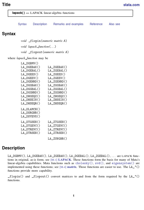
Title lapack()—LAPACK linear-algebra functionsSyntax Description Remarks and examples Reference Also seeSyntaxvoid flopin(numeric matrix A)void lapack function(...)void flopout(numeric matrix A)where lapack function may beLA DGBMV()LA DGEBAK()LA ZGEBAK()LA DGEBAL()LA ZGEBAL()LA DGEES()LA ZGEES()LA DGEEV()LA ZGEEV()LA DGEHRD()LA ZGEHRD()LA DGGBAK()LA ZGGBAK()LA DGGBAL()LA ZGGBAL()LA DGGHRD()LA ZGGHRD()LA DHGEQZ()LA ZHGEQZ()LA DHSEIN()LA ZHSEIN()LA DHSEQR()LA ZHSEQR()LA DLAMCH()LA DORGHR()LA DSYEVX()LA DTGSEN()LA ZTGSEN()LA DTGEVC()LA ZTGEVC()LA DTREVC()LA ZTREVC()LA DTRSEN()LA ZTRSEN()LA ZUNGHR()DescriptionLA DGBMV(),LA DGEBAK(),LA ZGEBAK(),LA DGEBAL(),LA ZGEBAL(),...are LAPACK func-tions in original,as-is form;see[M-1]LAPACK.These functions form the basis for many of Mata’s linear-algebra capabilities.Mata functions such as cholesky(),svd(),and eigensystem()are implemented using these functions;see[M-4]matrix.Those functions are easier to use.The LA*() functions provide more capability.flopin()and flopout()convert matrices to and from the form required by the LA*() functions.12lapack()—LAPACK linear-algebra functionsRemarks and examples LAPACK stands for Linear Algebra PACK age and is a freely available set of Fortran90routines for solving systems of simultaneous equations,eigenvalue problems,and singular-value problems.The original Fortran routines have six-letter names like DGEHRD,DORGHR,and so on.The Mata functions LA DGEHRD(),LA DORGHR(),etc.,are a subset of the LAPACK double-precision real and complex routine.All LAPACK double-precision functions will eventually be made available.Documentation for the LAPACK routines can be found at /lapack/,although we recommend obtaining LAPACK Users’Guide by Anderson et al.(1999).Remarks are presented under the following headings:Mapping calling sequence from Fortran to MataFlopping:Preparing matrices for LAPACKWarning on the use of rows()and cols()afterﬂopin()Warning:It is your responsibility to check infoExampleMapping calling sequence from Fortran to MataLAPACK functions are named withﬁrst letter S,D,C,or Z.S means single-precision real,D means double-precision real,C means single-precision complex,and Z means double-precision complex.Mata provides the D*and Z*functions.The LAPACK documentation is in terms of S*and C*.Thus,toﬁnd the documentation for LA DGEHRD,you must look up SGEHRD in the original documentation.The documentation(Anderson et al.1999,227)reads,in part,SUBROUTINE SGEHRD(N,ILO,IHI,A,LDA,TAU,WORK,LWORK,INFO)INTEGER IHI,ILO,INFO,LDA,LWORK,NREAL A(LDA,*),TAU(*),WORK(LWORK)and the documentation states that SGEHDR reduces a real,general matrix,A,to upper Hessenberg form,H,by an orthogonal similarity transformation:Q ×A×Q=H.The corresponding Mata function,LA DGEHRD(),has the same arguments.In Mata,arguments ihi, ilo,info,lda,lwork,and n are real scalars.Argument A is a real matrix,and arguments tau and work are real vectors.You can read the rest of the original documentation toﬁnd out what is to be placed(or returned) in each argument.It turns out that A is assumed to be dimensioned LDA×something and that the routine works on A(1,1)(using Fortran notation)through A(N,N).The routine also needs work space,which you are to supply in vector WORK.In the standard LAPACK way,LAPACK offers you a choice:you can preallocate WORK,in which case you have to choose a fairly large dimension for it, or you can do a query toﬁnd out how large the dimension needs to be for this particular problem.If you preallocate,the documentation reveals that the WORK must be of size N,and you set LWORK equal to N.If you wish to query,then you make WORK of size1and set LWORK equal to−1.The LAPACK routine will then return in theﬁrst element of WORK the optimal size.Then you call the function again with WORK allocated to be the optimal size and LWORK set to equal the optimal size.Concerning Mata,the above works.You can follow the LAPACK documentation to the e J()to allocate matrices or vectors.Alternatively,you can specify all sizes as missing value(.),and Mata willﬁll in the appropriate value based on the assumption that you are using the entire matrix.lapack()—LAPACK linear-algebra functions3 Thus,in LA DGEHRD(),you could specify lda as missing,and the function would run as if you had speciﬁed lda equal to cols(A).You could specify n as missing,and the function would run as if you had speciﬁed n as rows(A).Work areas,however,are treated differently.You can follow the standard LAPACK convention outlined above;or you can specify the sizes of work areas(lwork)and specify the work areas themselves (work)as missing values,and Mata will allocate the work areas for you.The allocation will be as you speciﬁed.One feature provided by some LAPACK functions is not supported by the Mata implementation.If a function allows a function pointer,you may not avail yourself of that option.Flopping:Preparing matrices for LAPACKThe LAPACK functions provided in Mata are the original LAPACK functions.Mata,which is C based, stores matrices PACK,which is Fortran based,stores matrices columnwise.Mata and Fortran also disagree on how complex matrices are to be organized.Functions flopin()and flopout()handle these issues.Coding flopin(A)changes matrixA from the Mata convention to the LAPACK convention.Coding flopout(A)changes A from theLAPACK convention to the Mata convention.The LA*()functions do not do this for you because LAPACK often takes two or three LAPACK functions run in sequence to achieve the desired result,and it would be a waste of computer time to switch conventions between calls.Warning on the use of rows()and cols()afterﬂopin()Be careful using the rows()and cols()functions.rows()of aﬂopped matrix returns the logical number of columns and cols()of aﬂopped matrix returns the logical number of rows!The danger of confusion is especially great when using J()to allocate work areas.If a LAPACK function requires a work area of r×c,you code,LA function(...,J(c,r,.),...)Warning:It is your responsibility to check infoThe LAPACK functions do not abort with error on failure.They instead store0in info(usually the last argument)if successful and store an error code if not successful.The error code is usually negative and indicates the argument that is a problem.ExampleThe following example uses the LAPACK function DGEHRD to obtain the Hessenberg form of matrixA.We will begin with1234112342456737891048910114lapack()—LAPACK linear-algebra functionsTheﬁrst step is to use flopin()to put A in LAPACK order::_flopin(A)Next we make a work-space query to get the optimal size of the work area.:LA_DGEHRD(.,1,4,A,.,tau=.,work=.,lwork=-1,info=0):lwork=work[1,1]:lwork128After putting the work-space size in lwork,we can call LA DGEHRD()again to perform the Hessenberg decomposition::LA_DGEHRD(.,1,4,A,.,tau=.,work=.,lwork,info=0)LAPACK function DGEHRD saves the result in the upper triangle and theﬁrst subdiagonal of A.We must use flopout()to change that back to Mata order,andﬁnally,we extract the result: :_flopout(A):A=A-sublowertriangle(A,2):A123411-5.370750529.0345341258.39223227032-11.3578166925.18604651-4.40577178-.656148389930-1.660145888-.1860465116.1760901813400-8.32667e-16-5.27356e-16ReferenceAnderson,E.,Z.Bai,C.Bischof,S.Blackford,J.Demmel,J.J.Dongarra,J.Du Croz,A.Greenbaum,S.Hammarling,A.McKenney,and PACK Users’Guide.3rd ed.Philadelphia:Society for Industrial andApplied Mathematics.Also see[M-1]LAPACK—The LAPACK linear-algebra routines[R]copyright lapack—LAPACK copyright notiﬁcation[M-4]matrix—Matrix functions。

线性代数—Linear Algebra

(ii)
1 A = − 1 2
1 −2 3
2 1
3 2
1 − 1 2 1 4 3
2 − 3 = LDLT 1
= ( L D )( L D )T = R T R
2011/6/13 13
Positive Definite Matrices: A=RTR R has independent columns
When the first derivatives əf/əx and əf/əy are zero and the second derivative matrix is positive definite, we have found a local minimum.
2011/6/13 6
6.5 Positive Definite Matrices(正定矩陣)
2011/6/13 7
6.5 Positive Definite Matrices:
First Application: Test for a Minimum
1 2 例題： A = 2 7
f(x,y)=xTAx=x2+4xy+7y2= (x+2y)2+3y2 >0 寫成兩個平方項之和。
a b 針對一般 A = b c
b 2 b2 2 f ( x, y ) = ax 2 + 2bxy + cy 2 = a ( x + y ) + (c − ) y a a
two pivots
2011/6/13
8
6.5 Positive Definite Matrices: First Application: Test for a Minimum

R2jags包用户指南说明书

Package‘R2jags’October12,2022Version0.7-1Date2021-08-05Title Using R to Run'JAGS'Author Yu-Sung Su<*********************.cn>,Masanao Yajima<*************>,Maintainer Yu-Sung Su<*********************.cn>BugReports https:///suyusung/R2jags/issues/Depends R(>=2.14.0),rjags(>=3-3)Imports abind,coda(>=0.13),graphics,grDevices,methods,R2WinBUGS,parallel,stats,utilsSystemRequirements JAGS()Description Providing wrapper functions to implement Bayesian analysis in JAGS.Some major fea-tures include monitoring convergence of a MCMC model using Rubin and Gelman Rhat statis-tics,automatically running a MCMC model till it converges,and implementing parallel process-ing of a MCMC model for multiple chains.License GPL(>2)RoxygenNote7.1.1Suggests testthat(>=3.0.0)Conﬁg/testthat/edition3NeedsCompilation noRepository CRANDate/Publication2021-08-0504:20:38UTCR topics documented:attach.jags (2)autojags (3)jags (4)jags2bugs (9)recompile (10)traceplot (11)12attach.jags Index12attach.jags Attach/detach elements of‘JAGS’objects to search pathDescriptionThese are wraper functions for attach.bugs and detach.bugs,which attach or detach three-way-simulation array of bugs object to the search path.See attach.all for details.Usageattach.jags(x,overwrite=NA)detach.jags()Argumentsx An rjags object.overwrite If TRUE,objects with identical names in the Workspace(.GlobalEnv)that are masking objects in the database to be attached will be deleted.If NA(the default)and an interactive session is running,a dialog box asks the user whether maskingobjects should be deleted.In non-interactive mode,behaviour is identical tooverwrite=FALSE,i.e.nothing will be deleted.DetailsSee attach.bugs for detailsAuthor(s)Yu-Sung Su<*********************.cn>,ReferencesSibylle Sturtz and Uwe Ligges and Andrew Gelman.(2005).“R2WinBUGS:A Package for Run-ning WinBUGS from R.”Journal of Statistical Software3(12):1–6.Examples#See the example in?jags for the usage.autojags3 autojags Function for auto-updating‘JAGS’until the model convergesDescriptionThe autojags takes a rjags object as input.autojags will update the model until it converges. Usage##S3method for class rjagsupdate(object,n.iter=1000,n.thin=1,refresh=n.iter/50,progress.bar="text",...) autojags(object,n.iter=1000,n.thin=1,Rhat=1.1,n.update=2,refresh=n.iter/50,progress.bar="text",...)Argumentsobject an object of rjags class.n.iter number of total iterations per chain,default=1000n.thin thinning rate.Must be a positive integer,default=1...further arguments pass to or from other methods.Rhat converegence criterion,default=1.1.n.update the max number of updates,default=2.refresh refresh frequency for progress bar,default is n.iter/50progress.bar type of progress bar.Possible values are“text”,“gui”,and“none”.Type“text”is displayed on the R console.Type“gui”is a graphical progress bar in a newwindow.The progress bar is suppressed if progress.bar is“none”Author(s)Yu-Sung Su<*********************.cn>ReferencesGelman,A.,Carlin,J.B.,Stern,H.S.,Rubin,D.B.(2003):Bayesian Data Analysis,2nd edition, CRC Press.Examples#see?jags for an example.4jags jags Run‘JAGS’from RDescriptionThe jags function takes data and starting values as input.It automatically writes a jags script,calls the model,and saves the simulations for easy access in R.Usagejags(data,inits,parameters.to.save,model.file="model.bug",n.chains=3,n.iter=2000,n.burnin=floor(n.iter/2),n.thin=max(1,floor((n.iter-n.burnin)/1000)),DIC=TRUE,working.directory=NULL,jags.seed=123,refresh=n.iter/50,progress.bar="text",digits=5,RNGname=c("Wichmann-Hill","Marsaglia-Multicarry","Super-Duper","Mersenne-Twister"),jags.module=c("glm","dic"),quiet=FALSE)jags.parallel(data,inits,parameters.to.save,model.file="model.bug",n.chains=2,n.iter=2000,n.burnin=floor(n.iter/2),n.thin=max(1,floor((n.iter-n.burnin)/1000)),n.cluster=n.chains,DIC=TRUE,working.directory=NULL,jags.seed=123,digits=5,RNGname=c("Wichmann-Hill","Marsaglia-Multicarry","Super-Duper","Mersenne-Twister"),jags.module=c("glm","dic"),export_obj_names=NULL,envir=.GlobalEnv)jags2(data,inits,parameters.to.save,model.file="model.bug",n.chains=3,n.iter=2000,n.burnin=floor(n.iter/2),n.thin=max(1,floor((n.iter-n.burnin)/1000)),DIC=TRUE,jags.path="",working.directory=NULL,clearWD=TRUE,refresh=n.iter/50)Argumentsdata(1)a vector or list of the names of the data objects used by the model,(2)a (named)list of the data objects themselves,or(3)the name of a"dump"formatﬁle containing the data objects,which must end in".txt",see example below fordetails.jags5 inits a list with n.chains elements;each element of the list is itself a list of start-ing values for the BUGS model,or a function creating(possibly random)initialvalues.If inits is NULL,JAGS will generate initial values for parameters.parameters.to.savecharacter vector of the names of the parameters to save which should be moni-tored.model.fileﬁle containing the model written in BUGS code.Alternatively,as in R2WinBUGS,model.file can be an R function that contains a BUGS model that is written toa temporary modelﬁle(see tempfile)using write.modeln.chains number of Markov chains(default:3)n.iter number of total iterations per chain(including burn in;default:2000)n.burnin length of burn in,i.e.number of iterations to discard at the beginning.Defaultis n.iter/2,that is,discarding theﬁrst half of the simulations.If n.burnin is0,jags()will run100iterations for adaption.n.cluster number of clusters to use to run parallel chains.Default equals n.chains.n.thin thinning rate.Must be a positive integer.Set n.thin>1to save memoryand computation time if n.iter is large.Default is max(1,floor(n.chains*(n.iter-n.burnin)/1000))which will only thin if there are at least2000simulations.DIC logical;if TRUE(default),compute deviance,pD,and DIC.The rule pD=var(deviance) /2is used.working.directorysets working directory during execution of this function;This should be thedirectory where modelﬁle is.jags.seed random seed for JAGS,default is123.This function is used for jags.parallell()and does not work for jags().Use set.seed()instead if you want to produceidentical result with jags().jags.path directory that contains the JAGS executable.The default is“”.clearWD indicating whether theﬁles‘data.txt’,‘inits[1:n.chains].txt’,‘codaIndex.txt’,‘jagsscript.txt’,and‘CODAchain[1:nchains].txt’should be removed af-ter jags hasﬁnished,default=TRUE.refresh refresh frequency for progress bar,default is n.iter/50progress.bar type of progress bar.Possible values are“text”,“gui”,and“none”.Type“text”is displayed on the R console.Type“gui”is a graphical progress bar in a newwindow.The progress bar is suppressed if progress.bar is“none”digits as in write.model in the R2WinBUGS package:number of signiﬁcant digitsused for BUGS input,see formatC.Only used if specifying a BUGS model as an Rfunction.RNGname the name for random number generator used in JAGS.There are four RNGS sup-plied by the base moduale in JAGS:Wichmann-Hill,Marsaglia-Multicarry,Super-Duper,Mersenne-Twisterjags.module the vector of jags modules to be loaded.Default are“glm”and“dic”.InputNULL if you don’t want to load any jags module.6jags export_obj_namescharacter vector of objects to export to the clusters.envir default is.GlobalEnvquiet Logical,whether to suppress stdout in jags.model().DetailsTo run:1.Write a BUGS model in an ASCIIﬁle.2.Go into R.3.Prepare the inputs for the jags function and run it(see Example section).4.The model will now run in JAGS.It might take awhile.You will see things happening in the Rconsole.BUGS version support:•jags1.0.3defaultAuthor(s)Yu-Sung Su<*********************.cn>,Masanao Yajima<********************.edu> ReferencesPlummer,Martyn(2003)“JAGS:A program for analysis of Bayesian graphical models using Gibbs sampling.”/plummer03jags.html.Gelman,A.,Carlin,J.B.,Stern,H.S.,Rubin,D.B.(2003)Bayesian Data Analysis,2nd edition, CRC Press.Sibylle Sturtz and Uwe Ligges and Andrew Gelman.(2005).“R2WinBUGS:A Package for Run-ning WinBUGS from R.”Journal of Statistical Software3(12):1–6.Examples#An example model file is given in:model.file<-system.file(package="R2jags","model","schools.txt")#Let s take a look:file.show(model.file)#you can also write BUGS model as a R function,see below:#=================##initialization##=================##dataJ<-8.0y<-c(28.4,7.9,-2.8,6.8,-0.6,0.6,18.0,12.2)sd<-c(14.9,10.2,16.3,11.0,9.4,11.4,10.4,17.6)jags7 jags.data<-list("y","sd","J")jags.params<-c("mu","sigma","theta")jags.inits<-function(){list("mu"=rnorm(1),"sigma"=runif(1),"theta"=rnorm(J))}##You can input data in4ways##1)data as list of characterjagsfit<-jags(data=list("y","sd","J"),inits=jags.inits,jags.params,n.iter=10,model.file=model.file)##2)data as character vector of namesjagsfit<-jags(data=c("y","sd","J"),inits=jags.inits,jags.params,n.iter=10,model.file=model.file)##3)data as named listjagsfit<-jags(data=list(y=y,sd=sd,J=J),inits=jags.inits,jags.params,n.iter=10,model.file=model.file)##4)data as a filefn<-"tmpbugsdata.txt"dump(c("y","sd","J"),file=fn)jagsfit<-jags(data=fn,inits=jags.inits,jags.params,n.iter=10,model.file=model.file)unlink("tmpbugsdata.txt")##You can write bugs model in R as a functionschoolsmodel<-function(){for(j in1:J){#J=8,the number of schoolsy[j]~dnorm(theta[j],tau.y[j])#data model:the likelihoodtau.y[j]<-pow(sd[j],-2)#tau=1/sigma^2}for(j in1:J){theta[j]~dnorm(mu,tau)#hierarchical model for theta}tau<-pow(sigma,-2)#tau=1/sigma^2mu~dnorm(0.0,1.0E-6)#noninformative prior on musigma~dunif(0,1000)#noninformative prior on sigma}jagsfit<-jags(data=jags.data,inits=jags.inits,jags.params,n.iter=10,model.file=schoolsmodel)#===============================##RUN jags and postprocessing##===============================#jagsfit<-jags(data=jags.data,inits=jags.inits,jags.params,n.iter=5000,model.file=model.file)#Run jags parallely,no progress bar.R may be frozen for a while,#Be patient.Currenlty update afterward does not run parallelly8jags #jagsfit.p<-jags.parallel(data=jags.data,inits=jags.inits,jags.params,n.iter=5000,model.file=model.file)#display the outputprint(jagsfit)plot(jagsfit)#traceplottraceplot(jagsfit.p)traceplot(jagsfit)#or to use some plots in coda#use as.mcmmc to convert rjags object into mcmc.listjagsfit.mcmc<-as.mcmc(jagsfit.p)jagsfit.mcmc<-as.mcmc(jagsfit)##now we can use the plotting methods from coda#require(lattice)#xyplot(jagsfit.mcmc)#densityplot(jagsfit.mcmc)#if the model does not converge,update it!jagsfit.upd<-update(jagsfit,n.iter=100)print(jagsfit.upd)print(jagsfit.upd,intervals=c(0.025,0.5,0.975))plot(jagsfit.upd)#before update parallel jags object,do recompile itrecompile(jagsfit.p)jagsfit.upd<-update(jagsfit.p,n.iter=100)#or auto update it until it converges!see?autojags for details#recompile(jagsfit.p)jagsfit.upd<-autojags(jagsfit.p)jagsfit.upd<-autojags(jagsfit)#to get DIC or specify DIC=TRUE in jags()or do the following#dic.samples(jagsfit.upd$model,n.iter=1000,type="pD")#attach jags object into search path see"attach.bugs"for detailsattach.jags(jagsfit.upd)#this will show a3-way array of the bugs.sim object,for example:mu#detach jags object into search path see"attach.bugs"for detailsdetach.jags()#to pick up the last save session#for example,load("RWorkspace.Rdata")recompile(jagsfit)jags2bugs9 jagsfit.upd<-update(jagsfit,n.iter=100)recompile(jagsfit.p)jagsfit.upd<-update(jagsfit,n.iter=100)#=============##using jags2##=============###jags can be run and produces coda files,but cannot be updated once it s done##You may need to edit"jags.path"to make this work,##also you need a write access in the working directory:##e.g.setwd("d:/")##NOT RUN HERE##Not run:jagsfit<-jags2(data=jags.data,inits=jags.inits,jags.params,n.iter=5000,model.file=model.file)print(jagsfit)plot(jagsfit)#or to use some plots in coda#use as.mcmmc to convert rjags object into mcmc.listjagsfit.mcmc<-as.mcmc.list(jagsfit)traceplot(jagsfit.mcmc)#require(lattice)#xyplot(jagsfit.mcmc)#densityplot(jagsfit.mcmc)##End(Not run)jags2bugs Read jags outputﬁles in CODA formatDescriptionThis function reads Markov Chain Monte Carlo output in the CODA format produced by jags and returns an object of class mcmc.list for further output analysis using the coda package.Usagejags2bugs(path=getwd(),parameters.to.save,n.chains=3,n.iter=2000,n.burnin=1000,n.thin=2,DIC=TRUE)Argumentspath sets working directory during execution of this function;This should be the directory where CODAﬁles are.10recompile parameters.to.savecharacter vector of the names of the parameters to save which should be moni-tored.n.chains number of Markov chains(default:3)n.iter number of total iterations per chain(including burn in;default:2000)n.burnin length of burn in,i.e.number of iterations to discard at the beginning.Defaultis n.iter/2,that is,discarding theﬁrst half of the simulations.n.thin thinning rate,default is2DIC logical;if TRUE(default),compute deviance,pD,and DIC.The rule pD=var(deviance) /2is used.Author(s)Yu-Sung Su<*********************.cn>,Masanao Yajima<********************.edu> recompile Function for recompiling rjags objectDescriptionThe recompile takes a rjags object as input.recompile will re-compile the previous saved rjagsobject.Usagerecompile(object,n.iter,refresh,progress.bar)##S3method for class rjagsrecompile(object,n.iter=100,refresh=n.iter/50,progress.bar="text")Argumentsobject an object of rjags class.n.iter number of iteration for adapting,default is100refresh refresh frequency for progress bar,default is n.iter/50progress.bar type of progress bar.Possible values are“text”,“gui”,and“none”.Type“text”is displayed on the R console.Type“gui”is a graphical progress bar in a newwindow.The progress bar is suppressed if progress.bar is“none”Author(s)Yu-Sung Su<*********************.cn>traceplot11Examples#see?jags for an example.traceplot Trace plot of bugs objectDescriptionDisplays a plot of iterations vs.sampled values for each variable in the chain,with a separate plot per variable.Usagetraceplot(x,...)##S4method for signature rjagstraceplot(x,mfrow=c(1,1),varname=NULL,match.head=TRUE,ask=TRUE,col=rainbow(x$n.chains),lty=1,lwd=1,...)Argumentsx A bugs objectmfrow graphical parameter(see par)varname vector of variable names to plotmatch.head matches the variable names by the beginning of the variable names in bugs ob-jectask logical;if TRUE,the user is ask ed before each plot,see par(ask=.).col graphical parameter(see par)lty graphical parameter(see par)lwd graphical parameter(see par)...further graphical parametersAuthor(s)Masanao Yajima<********************.edu>.See Alsodensplot,plot.mcmc,traceplotIndex∗IOjags2bugs,9∗ﬁlejags2bugs,9∗hplottraceplot,11∗interfaceattach.jags,2jags,4∗modelsautojags,3jags,4recompile,10attach.all,2attach.bugs,2attach.jags,2autojags,3densplot,11detach.bugs,2detach.jags(attach.jags),2 formatC,5jags,4jags2(jags),4jags2bugs,9mcmc.list,9plot.mcmc,11recompile,10rjags-class(jags),4rjags.parallel-class(jags),4 tempfile,5traceplot,11,11traceplot,bugs-method(traceplot),11traceplot,mcmc.list-method(traceplot),11traceplot,rjags-method(traceplot),11traceplot.default(traceplot),11update.rjags(autojags),3write.model,512。

Java中的闭包和Lambda表达式

Java中的闭包和Lambda表达式在Java编程语言中，闭包（closure）和Lambda表达式（Lambda expression）是两个非常重要的概念。

它们为我们提供了更加灵活和简洁的编程方式，大大提高了我们的代码效率和可读性。

本文将深入探讨Java中的闭包和Lambda表达式，并介绍它们的原理、使用方法以及常见应用场景。

一、闭包的概念与原理闭包是指一个函数（方法）加上其环境变量（lexical environment）组合而成的实体。

简单来说，闭包就是一个可调用的对象，它封装了某个具体函数的执行逻辑和其所需的外部变量。

闭包可以在被定义的环境结束后依然能够被调用，并且能够访问和修改其所引用的自由变量。

在Java中，闭包的实现依赖于匿名内部类或Lambda表达式。

在编写闭包时，需要注意以下几点：1. 外部变量必须是final或等效于final的（即值不可变）。

2. 外部变量的生命周期必须大于等于闭包的生命周期。

3. 闭包可以访问外部变量，并且在闭包内修改外部变量的值。

下面是一个示例代码，演示了闭包的基本用法：```public class ClosureExample {public static void main(String[] args) {int x = 10;Runnable r = () -> {System.out.println("Closure value: " + x);};r.run();}}```在上述代码中，我们定义了一个闭包r，它引用了外部变量x。

闭包在被调用时，能够访问并打印出外部变量x的值。

需要注意的是，外部变量x必须是final的或等效于final的。

闭包的一个重要应用场景是在多线程编程中。

由于闭包可以捕获外部的环境变量，并且在闭包内修改这些变量的值，我们可以使用闭包来实现线程安全的可变状态。

二、Lambda表达式的概念与使用方法Lambda表达式是Java 8中引入的一个重要特性，它允许以更加简洁的方式定义匿名函数。

java中使用克拉姆法则求解二元一次方程组

java中使用克拉姆法则求解二元一次方程组克拉姆法则又称为克拉默法则，是解决二元一次方程组的一种方法。

在Java中，可以通过编程实现克拉姆法则来求解该类方程组。

二元一次方程组的一般形式为：
ax + by = c
dx + ey = f
其中，a、b、c、d、e、f都是已知数，而x和y是未知数。

要解决这个方程组，需要求出x和y的值。

通过克拉姆法则，可以将上述方程组改写为以下形式：
x = (ce - bf) / (ae - bd)
y = (af - cd) / (ae - bd)
其中，分母是系数行列式，分子则是将系数矩阵中对应x或y的列替换为方程右边的常数向量后所得的行列式。

在Java中，可以通过定义系数矩阵和常数向量，再按照克拉姆法则的公式求解x和y的值。

具体实现可以使用数组或矩阵库来完成。

需要注意的是，克拉姆法则的主要优点是简单易懂，但是在实际计算中可能会出现精度误差。

因此，在使用克拉姆法则求解方程组时，需要注意对精度进行处理。

- 1 -。

lambda表达式数组循环

lambda表达式数组循环什么是lambda表达式？如何使用lambda表达式来进行数组循环？Lambda表达式是一种匿名函数，它可以在代码的任何地方被定义和使用。

它在很多编程语言中被广泛应用，包括Python、Java、C#等。

在数组循环中，lambda表达式可以用来定义一个函数，该函数将被用于迭代数组元素。

通过lambda表达式，我们可以更加简洁和灵活地编写循环代码。

下面将一步一步回答如何使用lambda表达式来进行数组循环。

第一步：理解lambda表达式的语法结构lambda表达式以关键字lambda开头，后面跟着参数列表，然后是冒号和一个函数体。

参数列表用括号括起来，多个参数之间用逗号分隔。

语法结构为：lambda 参数列表: 函数体第二步：了解lambda表达式的特点lambda表达式的特点是可以声明一个匿名函数，因此不需要给函数命名。

这种匿名函数通常用于简单的操作，而不需要定义一个命名函数。

第三步：使用lambda表达式进行数组循环在使用lambda表达式进行数组循环时，我们通常会结合内置函数（如map、filter等）或者循环语句（如for）来完成。

例如，如果我们有一个整数数组，我们想要将其中的每个元素都平方，可以使用lambda表达式和map函数来实现：nums = [1, 2, 3, 4, 5]squared_nums = list(map(lambda x: x2, nums))print(squared_nums)这段代码中，我们首先定义了一个整数数组nums，然后使用map函数和lambda表达式将每个元素平方。

最后，我们将平方后的结果转换成列表并打印出来。

第四步：使用lambda表达式筛选数组元素除了对数组元素进行处理，我们还可以使用lambda表达式来筛选数组元素。

例如，如果我们有一个整数数组，我们想要筛选出其中的偶数，可以使用lambda表达式和filter函数来实现：nums = [1, 2, 3, 4, 5]even_nums = list(filter(lambda x: x 2 == 0, nums))print(even_nums)这段代码中，我们首先定义了一个整数数组nums，然后使用filter函数和lambda表达式来筛选出其中的偶数。

java lambda list long转bigdecimal累加 -回复

java lambda list long转bigdecimal累加-回复Java Lambda 表达式是Java 8 引入的一种新的语法特性，可以简化匿名内部类的书写并使代码更加简洁。

它主要用于函数式编程，可以将函数作为方法的参数进行传递，使得代码更加灵活和可读性更高。

在实际的应用场景中，有时我们需要对一个Long 类型的集合进行累加操作，并且希望将结果存储为BigDecimal 类型。

本文将介绍如何使用Lambda 表达式和Stream API 来实现这一需求。

首先，我们需要创建一个包含Long 类型元素的List 集合，并将其存储为一个名为numbers 的变量。

javaList<Long> numbers = Arrays.asList(10L, 20L, 30L, 40L, 50L);接下来，我们使用Java 8 的Stream API 来对集合进行操作。

通过调用`stream()` 方法，我们可以将List 转换为一个流，从而可以使用Lambda 表达式进行操作。

javaBigDecimal sum = numbers.stream().map(BigDecimal::valueOf) 将Long 转换为BigDecimal.reduce(BigDecimal.ZERO, BigDecimal::add); 累加操作在上面的代码中，我们首先通过`map()` 方法将Long 类型的元素转换为BigDecimal 类型。

这里使用了方法引用`BigDecimal::valueOf` 来创建BigDecimal 对象。

然后，我们使用`reduce()` 方法对这些BigDecimal 对象进行累加操作，初始值设置为BigDecimal.ZERO，并使用`BigDecimal::add` 方法进行累加。

最后，我们将累加的结果存储在名为`sum` 的BigDecimal 对象中。

现在，`sum` 的值就是numbers 集合中所有元素的累加和。

javalambda循环_使用Java8Lambda简化嵌套循环操作

javalambda循环_使⽤Java8Lambda简化嵌套循环操作java lambda循环对于每个经常需要在Java 8（或更⾼版本）中使⽤多维数组的⼈来说，这只是⼀个快速技巧。

在这种情况下，您可能经常会以类似于以下代码的结尾：float[][] values = ...for (int i = 0; i < values.length; i++) {for (int k = 0; k < values[i].length; k++) {float value = values[i][k];// do something with i, k and value}}如果幸运的话，可以⽤for-each循环替换循环。

但是，循环内的计算通常需要索引。

在这种情况下，您可以提出⼀个简单的实⽤程序⽅法，如下所⽰：private void loop(float[][] values, BiConsumer<Integer, Integer> consumer) {for (int i = 0; i < values.length; i++) {for (int k = 0; k < values[i].length; k++) {consumer.accept(i, k);}}}现在，我们可以像这样循环遍历数组索引：float[][] values = ...loop(values, (i, k) -> {float value = values[i][k];// do something with i, k and value});这样，您可以使循环代码脱离主要逻辑。

当然，您应该更改所⽰的loop（）⽅法，使其适合您的个⼈需求。

补充知识：JAVA8-lambda表达式-并⾏流，提升效率的利器？写在前⾯的话在前⾯我们已经看过了⼀些流的处理，那么Lambda除了在写法上的不同，还有其它什么作⽤呢？当然有，就是数据并⾏化处理！它在某些场景下可以提⾼程序的性能。

Java解线性方程组

doubleSum=0.0;
for(intk=1;k<=r-1;k++)
Sum=Sum+a[i][k]*a[k][r];
returnSum;
}
publicstaticdoublejisuan2(inti){
doubleSum=0.0;
for(intk=1;k<=i-1;k++)
Sum=Sum+a[i][k]*x[k];
{
x[i]=f_x(i);
}
System.out.print(k+" ");
for(inti=1;i<=n;i++)
{
System.out.print(x[i]+" ");
}
System.out.println("\n");
}while(jisuan()>=e);
}
publicstaticdoublejisuan(){
}
}
publicstaticvoidDeterminant(){//求行列式
doubleDM=1.0;
for(inti=1;i<=n;i++)
{
doublea2=a[i][i];
DM=DM*a2;
}
doublen3=(double)n2;
DM=DM*Math.pow(-1.0, n3);
System.out.println("该方程组的系数行列式：det A = "+DM);
System.out.print(k+" ");
for(inti=1;i<=n;i++)

javapackage用法

javapackage用法Java中的package是一种组织类和接口的机制。

package可以包含多个类和子package，它们可以在同一包内或不同包内。

通过将类组合在一起，package可以使代码更加模块化，易于管理和维护。

在Java中，package的名字通常使用域名反转的方式来命名，例如com.mycompany.mypackage。

这可以确保package名称的唯一性，避免与其他包冲突。

若要在Java中使用package，需要在源代码文件的顶部添加package语句，并将文件保存在与package名称相同的文件夹内。

例如，若package名称为com.mycompany.mypackage，则该package的源代码文件应在com/mycompany/mypackage文件夹内，并在源代码文件的顶部添加package com.mycompany.mypackage语句。

在Java中，可以使用import语句来导入其他包中的类。

例如，若要使用java.util包中的ArrayList类，可以在源代码文件的顶部添加import java.util.ArrayList语句，然后在代码中就可以直接使用ArrayList类。

package还可以用于访问修饰符，Java中有public、protected、private和default四种访问修饰符，它们用于控制类、方法和变量的访问范围。

若不指定访问修饰符，则默认为default，只有在同一包内才能访问。

在Java中，package是一个重要的组织代码的方式，它可以使代码更加模块化、易于管理和维护。

了解和掌握javapackage的使用方法，对于Java程序员来说是非常重要的。

Catalan数,括号序列和栈

Catalan数,括号序列和栈全是⼊门的⼀些东西.基本全是从别处抄的.栈: ⽀持单端插⼊删除的线性容器. 也就是说,仅允许在其⼀端加⼊⼀个新元素或删除⼀个元素. 允许操作的⼀端也叫栈顶,不允许操作的⼀端也叫栈底.数个箱⼦相叠就可以认为是⼀个栈,只能在最顶端加⼊⼀个新箱⼦或拿⾛⼀个箱⼦.栈中的元素遵循后进先出(last in first out,LILO)的规律.即:更早出栈的元素,应为更早⼊栈者.这是⼀个演⽰:奇数⾏为栈中元素(右端可以进⾏插⼊删除),元素以逗号隔开, EMPTY表⽰栈为空偶数⾏为进⾏的操作EMPTY插⼊1010插⼊2010,20插⼊5110,20,51插⼊1010,20,51,10删除⼀个元素10,20,51删除⼀个元素10,20插⼊3010,20,30删除⼀个元素10,20删除⼀个元素10删除⼀个元素EMPTY栈混洗问题给出三个栈S1,S2,S3,⼀开始S1中含有1到n的n个数字且从栈顶到栈底数字依次为1,2,3,....n-1,n.只有两种允许的操作:A S1⾮空时从S1取出⼀个元素放⼊S2,B S2⾮空时可以从S2取出⼀个元素放⼊S3.最后S3中⾃底向上形成的序列称作⼀个栈混洗.例如,如果S1中⼀开始有1,2,3,4四个元素,那么先进⾏4次A操作再进⾏4次B操作,将得到序列4,3,2,1.如果A操作和B操作交替进⾏,将得到序列1,2,3,4.显然,栈混洗的结果并不唯⼀.⼀个长为n的序列的栈混洗可以表⽰成n次A操作和n次B操作组成的⼀个操作序列. ⽽n次A操作和n次B操作组成的⼀个操作序列也可以表⽰唯⼀的⼀个栈混洗序列.不同的操作序列必然得到不同的栈混洗,不同的栈混洗也必然对应不同的操作序列.并不是所有含有n个A,n个B的序列都是合理的操作序列.例如BBBBAAAA,将导致我们尝试拿出空栈S2中的元素.⼀个序列合理的条件是:对于任意m(1<=m<=2n),该序列的前m个操作中,B操作的数⽬不超过A操作的数⽬.只要满⾜这个条件就能保证任意时刻不会拿出空栈中的元素.如何判断⼀个栈混洗序列是否是可能出现的栈混洗序列例如,对于序列1,2,3,通过栈混洗可以得到[1,2,3],[3,2,1],[1,3,2],[2,1,3],[2,3,1],但是⽆法得到[3,1,2].如果使3最先出栈,那么就必须先令1,2⼊栈,从⽽2会在1之前出栈,只能得到[3,2,1]任意给出⼀个n和⼀个排列,如何判断这个排列能否通过栈混洗得到?例如,n=5,序列为5,4,1,3,2,是否可能?直接的思路是,直接根据我们要得到的序列,尝试进⾏A操作和B操作.例如,n=5时,要使序列的第⼀个元素为5,就必须⼀直进⾏A操作直到5出现在S2的栈顶.之后需要4,4恰好在S2的栈顶,于是弹出4.接下来需要的1不在栈顶,因此这个序列⽆法通过栈混洗得到.时间复杂度显然为O(n).其正确性也是显然的.栈混洗与括号序列⾸先只考虑由⼀种括号组成的括号序列.()()()(),(()())(),((()))都是能够匹配的括号序列.)(,))(,())(都是不能够匹配的括号序列.只要将A操作与左括号"("对应,B操作与右括号")"对应,栈混洗的合法操作序列就可以和能够匹配的括号序列⼀⼀对应.例如,AABB对应(()),ABAB对应()()按照我们之前的理解,如果保证序列中左右括号数⽬相同,那么我们只需要扫描⼀遍序列并维护⼀个计数器,初始为0,遇到左括号+1,遇到右括号-1,只要这个计数器的数值始终⾮负,就说明任意⼀个前缀中左括号的数⽬多于右括号的数⽬,等价于这个序列是能够匹配的括号序列.另⼀种判断括号序列是否合法的⽅法:初始化⼀个空栈S,从左向右扫描序列,遇到⼀个左括号将其⼊栈,遇到⼀个右括号时判断栈中是否有⼀个左括号,如果有,那么这个左括号与当前遇到的右括号相匹配.如果栈为空,那么这个括号序列并不合法.通过这种⽅式,我们除了得知括号序列是否合法,还可以得知每个右括号具体是和哪个左括号匹配,还可以处理序列中出现了多种括号且只有对应种类的括号能匹配的情况.可以⾃⾏尝试,"维护⼀个计数器"的⽅式并不能⽅便地扩展到多种括号的情况.拓展:允许循环移位的合法括号序列允许将括号序列的最左侧元素拿到最右边,问能否通过若⼲次这样的操作使得括号序列合法.⾸先这样的序列仍然需要满⾜左括号和右括号数⽬相同. 但是除此之外还需要满⾜什么条件呢?令⼈惊讶的是,除此之外并不需要满⾜什么条件.只要左括号和右括号数⽬相同,就可以保证能够通过若⼲次循环移位使得括号序列合法.给出⼀个构造⽅式:将左括号视为1,右括号视为-1,求取该序列的前缀和.如果前缀和中的最⼩值为0那么序列本⾝就是合法的.否则我们找到前缀和的最⼩值的出现位置(多个数值相同时取最左侧的),将这个位置之前的⼀段序列移位到右端,得到的即为合法的括号序列.构造⽅式的正确性不难证明.括号序列计数有多少个不同的含有n对括号的合法括号序列?这个问题等价于通过栈混洗可以得到多少个不同序列.也等价于,有多少个含有n个0,n个1的长为2n的字符串使得任意⼀个前缀中1的数⽬不少于0的数⽬.假设答案为f[n].边界条件为f[0]=1,表⽰没有括号/没有元素时也算有⼀种⽅案(空串也是⼀种合法序列).插播两条⾼中数学:分类加法计数原理:做⼀件事有m类⽅法,每类⽅法分别有A1,A2...Am种做法,那么做这件事共有A1+A2+...+Am种⽅法分步乘法计数原理:做⼀件事有m个步骤,每个步骤分别有A1,A2...Am种做法,那么做这件事共有A1∗A2∗...∗Am种⽅法好了,接下来我们来将所学的⽤于实践.考虑最左侧的左括号匹配的右括号在什么位置.假设这个左括号和匹配的右括号之间有2i个括号(这个数⽬必须是偶数),这2i个括号排列成合法括号序列的⽅案数为f[i].匹配的右括号右边还有2n-2i-2个括号,将它们排列为合法括号序列的⽅案数为f[n-i-1],这两部分可以认为是两个步骤,是独⽴的,那么总的⽅案数是f[i]*f[n-i-1].对于不同的i,我们可以认为是做⼀件事的不同种类的⽅法.于是f[1]=f[0]∗f[0],f[2]=f[1]∗f[0]+f[0]∗f[1],f[3]=f[0]∗f[2]+f[1]∗f[1]+f[2]∗f[0],这是⼀个O(n^2)的计算⽅式.这⾥我们得到的f[n]也叫Catalan数(卡特兰数),它还具有很多实际意义.紫书330~331页给出了Catalan数的另⼀个实际意义:多边形三⾓剖分数⽬,并通过另⼀个O(n^2)的递推公式,推倒了O(n)的递推公式.另⼀个常⽤的计算公式是f[n]=C(2n,n)/(n+1)=C(2n,n) - C(2n,n-1),C(2n,n)为组合数.catalan数的⼀个推⼴:n个左括号,m个右括号,任意前缀中左括号不少于右括号的序列数？答案是C(n+m,m)-C(n+m,m-1).Processing math: 100%。

1、下载文档前请自行甄别文档内容的完整性，平台不提供额外的编辑、内容补充、找答案等附加服务。
2、"仅部分预览"的文档,不可在线预览部分如存在完整性等问题,可反馈申请退款(可完整预览的文档不适用该条件!)。
3、如文档侵犯您的权益，请联系客服反馈,我们会尽快为您处理(人工客服工作时间：9:00-18:30)。

would become
MyInt z = x.operator plus(y);
2 Operator Overloading
We implemented a simple operator overloading facility for Java, based loosely on the overloading facilities of C++ 7] and on Gosling's proposal. Declaring an operator is just like declaring a method, except that the name of the method is the keyword operator followed the operator token. For instance,
A.set(i, j, A.get(i, j) + B.get(i, k) * C.get(k, j))
instead of the much more natural
A i,j] = A i,j] + B i,k] * C k,j]
Such a solution places to much of a burden of inconvenience upon the programmer, and would lead to programs that are di cult to understand and maintain. Therefore, we explored three options:
Contact address: IBM T.J. Watson Research Centeights, NY 10598, telephone (914) 784-7811, facsimile (914) 784-6576, email dfb@.
Changing the virtual machine interface by adding data types and bytecode operators to support multi-dimensional arrays in a \native" fashion. This solution also requires changing the Java-tobytecode compiler to support the new array operations. Extending the source language by adding array operations, and converting them into standard bytecodes and method calls. Modifying the way the virtual machine implements multi-dimensional arrays without changing the virtual machine interface. Initially we explored the third solution, since it was deemed that a solution which did not change the language semantics in any way was most desirable. It is possible to change the way multi-dimensional arrays are implemented so that the data is stored densely, with the object headers \out of line". While this would allow multi-dimensional arrays to be used in Java without changing the source language or VM interface, it only solves half of the problem: it is still not possible to represent sub-arrays. Therefore, this approach was reluctantly abandoned. The rst solution su ers from the fact that it requires changes throughout the system, requiring substantial programmer e ort, and is therefore unlikely to gain wide acceptance. We chose the second solution, namely changing the input language but compiling the array operations into method calls. Java-to-bytecode compilers are relatively simple, and because the bytecodes are portable, it would be possible to run the array codes on any machine, regardless of the presence of our modi ed compiler. We also decided to implement a general purpose solution to the problem: we provide generalized operator overloading for Java. The e ort required is not much larger then the e ort for a specialized solution, and by solving a wider problem of interest to more programmers, we increase the likelihood od broad-based acceptance. The generalized facility also makes it much easier to incorporate future improvements and modi cations that are demanded by experience. There are four components to JaLA: 1
JaLA: a Java package for Linear Algebra
David F. Bacon IBM T.J. Watson Research Center
1 Introduction
While the Java language has taken the world by storm, it has left the scienti c computing community out in the cold. Java lacks the capability for multi-dimensional arrays that can be implemented e ciently, and more importantly, lacks the ability to use data layouts that are compatible with the wide variety of scienti c subroutine packages available, such as the BLAS 3], ESSL 2], LAPACK 1], and so on. The problems stems from the fact that in Java, every non-scalar data item is an object, and every object must have an object header, typically two or three words long. Two-dimensional arrays are vector objects that contain a list of vector objects corresponding to the second dimension. Such a data organization is incompatible with the data layouts used by FORTRAN and C. Data access is also inherently less e cient because an extra indirection is required and it is impossible to traverse the array using a simple increment scheme. Java also lacks the ability to represent sub-arrays of any sort, or the ability to pass an array element by reference. Unfortunately, Java's extension capabilities are not su cient to provide the necessary functionality with a convenient syntax. If the native capabilities of Java were used to declare array classes, then programmers would be required to write programs like this:
Modi ed Java-to-bytecode compiler that extends the Java language with generalized operator overloading; Array class libraries that use the operator overloading facility to provide syntactically convenient array operations; Native method implementations of selected array operations that call scienti c subroutine libraries instead of performing the operation in Java (we used IBM's ESSL library); and A modi ed JNI (Java Native Interface) that takes advantage of special features of the array classes to reduce the cost of crossing the Java-to-native code barrier (optional).