Linear Approximation
MBA课程 线性规划 Linear Programing 英文原版

ASSUMPTIONS OF LINEAR PROGRAMMING •from a mathematical viewpoint, the assumptions simply are that the model must have a linear objective function subject to linear constraints.•However, from a modeling viewpoint, these mathematical properties of a linear programming model imply that certain assumptions must hold about the activities and data of the problem being modeled, including assumptions about the effect of varying the levels of the activities.•Proportionality •Additivity •Divisibility •CertaintyProportionality assumptioncosts•This case would arise if there were start-up costs associated with initiating the production of product 1. For example, there might be costs involved with setting up the production facilities. There might also be costs associated with arranging the distribution of the new product. Because these are one-time costs, they would need to be amortized on a per-week basis to be commensurable with Z (profit in thousands of dollars per week).costs•Suppose that this amortization were done and that the total start-up cost amounted to reducing Z by 1, but that the profit without considering the start-up cost would be 3x1. This would mean that the contribution from product 1 to Z should be 3x1-1 for x1 > 0, whereas the contribution would be 3x1 0 when x1 0 (no start-up cost). This profit function,3 which is given by the solid curve in Fig., certainly is not proportional to x1.increasing marginal return•the slope of the profit function for product 1 keeps increasing asx 1is increased. This violation of proportionality might occurbecause of economies of scale that can sometimes be achieved at higher levels of production, e.g., through the use of more efficient high-volume machinery, longer production runs, quantity discounts for large purchases of raw materials, and the learning-curve effect whereby workers become more efficient as they gain experience with a particular mode of production.As the incremental cost goes down, the incremental profit will go up (assuming constant marginal revenue).decreasing marginal return•the slope of the profit function for product 1 keeps decreasing as xis increased.1decreasing marginal return•the marketing costs need to go up more than proportionally to attain increases in the level of sales . For example, it might be possible to sell product 1 at the rate of 1 per week (x 1=1) with no advertising, whereas attaining sales to sustain a production rate of x 1=2 might require a moderate amount of advertising, x 1=3might necessitate an extensive advertising campaign, and x 1=4 might require also lowering the price•The conclusion was that proportionality could indeed be assumed without serious distortion.•what happens when the proportionality assumption does not hold even as a reasonable approximation? In most cases, this means you must use nonlinear programming instead• a certain important kind of nonproportionality can still be handled by linear programming by reformulating the problem appropriately.•Furthermore, if the assumption is violated only because of start-up costs, there is an extension of linear programming (mixed integer programming) that can be usedAdditivity•Although the proportionality assumption rules out exponents other than 1, it does not prohibit cross-product terms (terms involving the product of two or more variables).•Additivity assumption: Every function in a linear programming model (whether the objective function or the function on the left-hand side of a functional constraint) is the sum of the individual contributions of the respective activities•this case corresponds to an objective function of Z =3x1+5x2+x1x2, so that Z =3+ 5+ 1= 9 for (x1, x2) (1, 1), thereby violating the additivity assumption that Z =3+5.•The proportionality assumption still is satisfied since after the value of one variable is fixed, the increment in Z from the other variable is proportional to the value of that variable. This case would arise if the two products were complementary in some way that increases profit.•For example, suppose that a major advertising campaign would be required to market either new product produced by itself, but that the same single campaign can effectively promote both products if the decision is made to produce both. Because a major cost is saved for the second product, their joint profit is somewhat more than the sum of their individual profits when each is produced by itself.•Case 2 also violates the additivity assumption because of the extra term in the corresponding objective function, Z =3x 1+5x 2-x 1x 2, so that Z=3+5-1= 7 for (x 1, x 2) (1, 1). As the reverse of the first case, Case 2 would arise if the two products were competitive in some way that decreased their joint profit.•For example, suppose that both products need to use the same machinery and equipment . If either product were produced by itself, this machinery and equipment would be dedicated to this one use. However, producing both products would require switching the production processes back and forth, with substantial time and cost involved in temporarily shutting down the production of one product and setting up for the other.Affect the additivity of the constraint functions•Affect the additivity of the constraints function•For example, consider the third functional constraint of the Wyndor Glass Co. problem: 3x1+2x2<=18. (This is the only constraint involving both products.)•3x1+2x2+0.5x1x2<=18•namely, extra time is wasted switching the production processes back and forth between the two products. The extra cross-product term (0.5x1x2) would give the production time wastedin this way. (Note that wasting time switching between products leads to a positive cross-product term here, where the total function is measuring production time used, whereas it led to a negative cross-product term for Case 2 because the total function there measures profit.)•For Case 4 the function for production time used is 3x1+2x2-0.1x21x2, so the function value for (x1, x2)=(2, 3) is 6+6-1.2=10.8. This case could arise in the following way.•As in Case 3, suppose that the two products require the same type of machinery and equipment. But suppose now that the time required to switch from one product to the other would be relatively small.•occasional idle periodsDivisibility•Divisibility assumption: Decision variables in a linear programming model are allowed to have any values, including noninteger values, that satisfy the functional and nonnegativityconstraints. Thus, these variables are not restricted tojust integer values. Since each decision variable represents the level of some activity, it is being assumed that the activities can be run at fractional levels.Certainty•Certainty assumption: The value assigned to each parameter of a linear programming model is assumed to be a known constant •Linear programming models usually are formulated to select some future course of action. Therefore, the parameter values used would be based on a prediction of future conditions, which inevitably introduces some degree of uncertainty.•sensitivity analysis to identify the sensitive parameters•other ways of dealing with linear programming under uncertainty•It is very common in real applications of linear programming that almost none of the four assumptions hold completely. Except perhaps for the divisibility assumption, minor disparities are to be expected.This is especially true for the certainty assumption, so sensitivity analysis normally is a must to compensate for the violation of this assumption•A disadvantage of these other models is that the algorithms available for solving them are not nearly as powerful as those for linear programming, but this gap has been closing in some cases. For some applications, the powerful linear programming approach is used for the initial analysis, and then a more complicated model is used to refine this analysisThe Simplex MethodTHE ESSENCE OF THE SIMPLEX METHOD •The simplex method is an algebraic procedure. However, its underlying concepts are geometric.•Before delving into algebraic details, we focus in this section on the big picture from a geometric viewpoint.•each constraint boundary is a line that forms the boundary of what is permitted by the corresponding constraint. The points of intersection are the corner-point solutions of the problem. The five that lie on the corners of the feasible region—(0, 0), (0, 6), (2, 6), (4, 3), and (4, 0)—are the cornerpoint feasible solutions (CPF solutions). [The other three—(0, 9), (4, 6), and (6, 0)—are called corner-point infeasible solutions.]•In this example, each corner-point solution lies at the intersection of two constraint boundaries.•For a linear programming problem with n decision variables, each of its cornerpoint solutions lies at the intersection of n constraint boundaries.•Certain pairs of the CPF solutions share a constraint boundary, and other pairs do not.•For any linear programming problem with n decision variables, two CPF solutions are adjacent to each other if they share n-1 constraint boundaries. The two adjacent CPF solutions are connected by a line segment that lies on these same shared constraint boundaries. Such a line segment is referred to as an edge of the feasible region•Since n=2 in the example, two of its CPF solutions are adjacent if they share one constraint boundary; for example, (0, 0) and (0, 6) are adjacent because they share the x1=0 constraint boundary. The feasible region in Fig has five edges, consisting of thefive line segments forming the boundary of this region. Note that two edges emanate from each CPF solution. Thus, each CPF solution has two adjacent CPF solutions•Optimality test: Consider any linear programming problem that possesses at least one optimal solution. If a CPF solution has no adjacent CPF solutions that are better (as measured by Z), thenit must be an optimal solutionSolving the Example -Wyndor Glass Co. Problem•Initialization: Choose (0, 0) as the initialCPF solution to examine. (This is aconvenient choice because no calculationsare required to identify this CPF solution.)•Optimality Test: Conclude that (0, 0) is notan optimal solution. (Adjacent CPFsolutions are better.)•Iteration 1: Move to a better adjacent CPFsolution, (0, 6), by performing the followingthree steps.•1. Considering the two edges of the feasible region that emanate from (0, 0), choose to move along the edge that leads up the x 2axis. (With an objective function of Z=3x 1+5x 2, moving up the x 2axis increases Z at afaster rate than moving along the x 1axis.)•2. Stop at the first new constraint boundary:2x 2=12. [Moving farther in the directionselected in step 1 leaves the feasible region; e.g., moving to the second new constraint boundary hit when moving in that direction gives (0, 9), which is a corner-point infeasible solution.]•3. Solve for the intersection of the new set of constraint boundaries: (0, 6). (The equations for these constraint boundaries, x 1=0 and 2x 2=12, immediately yield this solution.)•Optimality Test: Conclude that (0, 6) is not an optimal solution. (An adjacent CPF solution is better.)•Iteration 2: Move to a better adjacent CPF solution, (2, 6), by performing the following three steps•1. Considering the two edges of the feasible region that emanate from (0, 6), choose tomove along the edge that leads to the right. (Moving along this edge increases Z, whereas backtracking to move back down the x2axis decreases Z.)2. Stop at the first new constraint boundary encountered when moving in that direction:3x1+2x2=12. (Moving farther in the direction selected in step 1 leaves the feasibleregion.)3. Solve for the intersection of the new set of constraint boundaries: (2, 6). (The equations for these constraint boundaries, 3x1+2x2=18 and2x2=12, immediately yield this solution.)•Optimality Test: Conclude that (2, 6) is an optimal solution, so stop. (None of the adjacent CPF solutions are better.)The Key Solution Concepts•Solution concept 1: The simplex method focuses solely on CPF solutions. For any problem with at least one optimal solution, finding one requires only finding•The only restriction is that the problem must possess CPF solutions. This is ensured if the feasible region is bounded.•Solution concept 2: The simplex method is an iterative algorithm (a systematic solution procedure that keeps repeating a fixed series of steps, called an iteration, until a desired result has been obtained) with the following structure.•Solution concept 3: Whenever possible, the initialization of the simplex method chooses the origin (all decision variables equal to zero) to be the initial CPF solution. When there are too many decision variables to find an initial CPF solution graphically, this choice eliminates the need to use algebraic procedures tofind and solve for an initial CPF solution•Solution concept 4: Given a CPF solution, it is much quicker computationally to gather information about its adjacent CPF solutions than about other CPF solutions. Therefore, each time the simplex method performs an iteration to move from the current CPF solution to a better one, it always chooses a CPF solution that is adjacent to the current one. No other CPF solutions are considered. Consequently, the entire path followed to eventually reach an optimal solution is alongthe edges of the feasible region.•Solution concept 5: After the current CPF solution is identified, the simplex method examines each of the edges of the feasibleregion that emanate from this CPF solution. Each of theseedges leads to an adjacent CPF solution at the other end, but the simplex method does not even take the time to solve for theadjacent CPF solution. Instead, it simply identifies the rate of improvement in Z that would be obtained by moving along the edge. Among the edges with a positive rate of improvement in Z, it then chooses to move along the one with the largest rate of improvement in Z. The iteration is completed by first solving for the adjacent CPF solution at the other end of this one edge and then relabeling this adjacent•Solution concept 6: Solution concept 5 describes how the simplex method examines each of the edges of the feasible region that emanate from the current CPF solution. This examination of an edge leads to quickly identifying the rate of improvement in Z that would be obtained by moving along the edge toward theadjacent CPF solution at the other end. A positive rate of improvement in Z implies that the adjacent CPF solution is better than the current CPF solution, whereas a negative rate of improvement in Z implies that the adjacent CPF solution is worse. Therefore, the optimality test consists simply of checking whether any of the edges give a positive rate of improvement in Z. If none do, then the current CPF solution is optimalSETTING UP THE SIMPLEX METHOD•The algebraic procedure is based on solving systems of equations. Therefore, the first step in setting up the simplex method is to convert the functional inequality constraints to equivalent equality constraints. (The nonnegativity constraints are left asinequalities because they are treated separately.) This conversion is accomplished by introducing slack variables.•Although both forms of the model represent exactly the same problem, the new form is much more convenient for algebraic manipulation and for identification of CPF solutions.•We call this the augmented form of the problem because the original form has been augmented by some supplementary variables neededto apply the simplex method.。
Linear Programming for Optimization
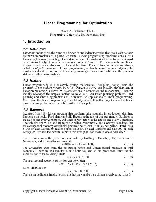
1 .1 Definition Linear programming is the name of a branch of applied mathematics that deals with solving optimization problems of a particular form. Linear programming problems consist of a linear cost function (consisting of a certain number of variables) which is to be minimized or maximized subject to a certain number of constraints. The constraints are linear inequalities of the variables used in the cost function. The cost function is also sometimes called the objective function. Linear programming is closely related to linear algebra; the most noticeable difference is that linear programming often uses inequalities in the problem statement rather than equalities. 1 .2 History Linear programming is a relatively young mathematical discipline, dating from the invention of the simplex method by G. B. Dantzig in 1947. Historically, development in linear programming is driven by its applications in economics and management. Dantzig initially developed the simplex method to solve U.S. Air Force planning problems, and planning and scheduling problems still dominate the applications of linear programming. One reason that linear programming is a relatively new field is that only the smallest linear programming problems can be solved without a computer. 1 .3 Example (Adapted from [1].) Linear programming problems arise naturally in production planning. Suppose a particular Ford plant can build Escorts at the rate of one per minute, Explorer at the rate of one every 2 minutes, and Lincoln Navigators at the rate of one every 3 minutes. The vehicles get 25, 15, and 10 miles per gallon, respectively, and Congress mandates that the average fuel economy of vehicles produced be at least 18 miles per gallon. Ford loses $1000 on each Escort, but makes a profit of $5000 on each Explorer and $15,000 on each Navigator. What is the maximum profit this Ford plant can make in one 8-hour day?
LinearApproximations,Differentials线性逼近微分解读

1.5
1 2 f x x 3 2
f x x
1.5
Guess:
2
z 3
(not drawn to scale)
3 1 2 f 3 3 3 1.5 2
mtangent f 3 3
1.5 3 z 1.5 z 3
1.5 3 2.5 (new guess) 3
Looking for this root.
Bad guess.
Wrong root found
Failure to converge
Newton’s method is built in to the Calculus Tools application on the TI-89.
Of course if you have a TI-89, you could just use the root finder to answer the problem. The only reason to use the calculator for Newton’s Method is to help your understanding or to check your work.
x1 a
y1 f a
m f a
y f a f a x a y f a f a x a L x f a f a x a
linearization of f at a
It is sometimes called the Newton-Raphson method
This is a recursive algorithm because a set of steps are repeated with the previous answer put in the next repetition. Each repetition is called an iteration.
自动化中英文对照表
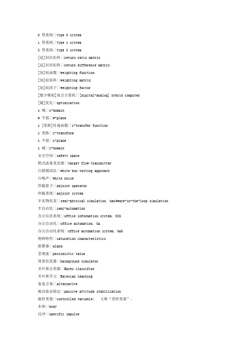
0 型系统||type 0 system1 型系统||type 1 system2 型系统||type 2 system[返]回比矩阵||return ratio matrix[返]回差矩阵||return difference matrix[加]权函数||weighting function[加]权矩阵||weighting matrix[加]权因子||weighting factor[数字模拟]混合计算机||[digital-analog] hybrid computer[最]优化||optimizations 域||s-domainw 平面||w-planez [变换]传递函数||z-transfer functionz 变换||z-transformz 平面||z-planez 域||z-domain安全空间||safety space靶式流量变送器||target flow transmitter白箱测试法||white box testing approach白噪声||white noise伴随算子||adjoint operator伴随系统||adjoint system半实物仿真||semi-physical simulation, hardware-in-the-loop simulation 半自动化||semi-automation办公信息系统||office information system, OIS办公自动化||office automation, OA办公自动化系统||office automation system, OAS饱和特性||saturation characteristics报警器||alarm悲观值||pessimistic value背景仿真器||background simulator贝叶斯分类器||Bayes classifier贝叶斯学习||Bayesian learning备选方案||alternative被动姿态稳定||passive attitude stabilization被控变量||controlled variable; 又称“受控变量”。
医学统计学(李琳琳)7相关分析与回归分析-2023年学习资料

【解析】-研究目的:凝血酶浓度和凝血时间两定量-之间是否存在线性关系,其联系程度如何?
一绘制散点图-从整体趋势而言,-1-15-随着凝血酶浓度的-413-增加,凝血时间呈-12-11-降低的趋 ,且二-10-0.7-0.8-0.9-1.1-1.2-1.3-者之间存在线性相-图7-5凝血酶浓度X与凝血 间Y散点图-关关系。
p的假设检验-H0:p=0-H1:P≠0-a=0.05-1查表法-由前面计算得:样本相关系数r=-0.90 ;-对给定a=0.05,自由度n-2=13,有附表11P391-查临界值r0.0513=0.560;-因为 0.907>0.560,则K0.05,拒绝H,即认-为变量X与Y间的线性相关关系有统计学意义。
2t检验-Ho:p=0-H1:p0-a=0.05--0.907-t,=-=-7.765-1-r2-1-0. 0702-n-2-15-2-y=15-2=13-查t界值表,1,>ts.13=2.160P<0.05,按a 0.05水准,拒-绝HO,接受H1,可认为凝血时间的长短与凝血酶浓度呈负粗-关。
相关系数的大小示意图-3.6-活-3.4-r=1-y-3230-0<r<1-L-8-r=0-2.6-2.4 2.2-40-42444648505254565860-体重kg,X
二、相关系数的意义与计算-若双变量X与Y均是来自正态总体的随机变量,散-点图呈线性趋势,且各观察值相互独立 则两变量-之间的相关关系可采用Pearson积矩相关系数表示。-∑X-XY-Y-∑x-X2∑Y-2xm
P391-附表11相关系数r临界值表-样本大小-0.05-0.01-1.000-6-0.88G-7-0T8 -0.929-0,738-0.881-0.700-0.833-10-0.648-0.794-0.618-0 755-12-0.587-0.727-13-0.560-0.703-0.538-0.679-15-0.52 -0.G54
Gamma1
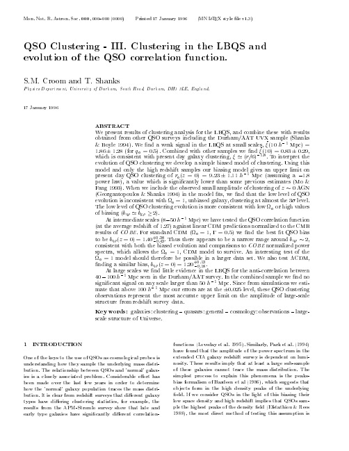
Printed 17 January 1996
A (MN L TEX style le v1.3)
QSO Clustering - III. Clustering in the LBQS and evolution of the QSO correlation function.
One of the keys to the use of QSOs as cosmological probes is understanding how they sample the underlying mass distribution. The relationship between QSOs and 'normal' galaxies is a closely associated problem. Considerable e ort has been made over the last few years in order to determine how the 'normal' galaxy population traces the mass distribution. It is clear from redshift surveys that di erent galaxy types have di ering clustering statistics, for example, the results from the APM-Stromlo survey show that late and early type galaxies have signi cantly di erent correlationfunctions (Loveday et al. 1995). Similarly, Park et al. (1994) have found that the amplitude of the power spectrum in the extended CfA galaxy redshift sБайду номын сангаасrvey is dependent on luminosity. These results imply that at least a large sub-sample of these galaxies cannot trace the mass distribution. The simplest process to explain this phenomena is the peaksbias formalism of Bardeen et al (1986), which suggests that objects form in the high density peaks of the underlying eld. If we consider QSOs in the light of this biasing their low space density and high redshift implies that QSOs sample the highest peaks of the density eld (Efstathiou & Rees 1988), the most direct method of testing this assumption is
计量经济学中英文词汇对照
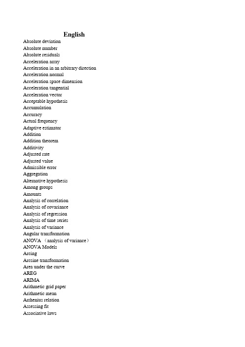
Common variance Common variation Communality variance Comparability Comparison of bathes Comparison value Compartment model Compassion Complement of an event Complete association Complete dissociation Complete statistics Completely randomized design Composite event Composite events Concavity Conditional expectation Conditional likelihood Conditional probability Conditionally linear Confidence interval Confidence limit Confidence lower limit Confidence upper limit Confirmatory Factor Analysis Confirmatory research Confounding factor Conjoint Consistency Consistency check Consistent asymptotically normal estimate Consistent estimate Constrained nonlinear regression Constraint Contaminated distribution Contaminated Gausssian Contaminated normal distribution Contamination Contamination model Contingency table Contour Contribution rate Control
linearsvr参数
linearsvr参数LinearSVR是支持向量机回归的一个线性模型,用于解决回归问题。
它的参数有以下几个:1. C(float,默认为1.0):惩罚系数,控制错误项的惩罚程度。
C越小,容忍错误项越多,模型的复杂度也相应降低;C越大,容忍错误项越少,模型的复杂度也相应增加。
2. epsilon(float,默认为0.1):ε不敏感损失函数中的最大容忍度。
如果预测值与真实值之间的差小于epsilon,则该样本的误差被视为0;否则,样本的误差等于差的绝对值减去epsilon。
3. tol(float,默认为1e-4):停止训练的容忍度。
当前后两次迭代之间的损失函数值差的绝对值小于tol时,停止继续迭代。
4. loss({'epsilon_insensitive','squared_epsilon_insensitive'},默认为'epsilon_insensitive'):损失函数的类型。
'epsilon_insensitive'表示ε不敏感损失函数,'squared_epsilon_insensitive'表示平方ε不敏感损失函数。
5. fit_intercept(bool,默认为True):是否计算截距项。
如果为True,则模型会计算并使用截距项;如果为False,则模型不会计算截距项。
6. intercept_scaling(float,默认为1):计算截距项时的缩放因子。
7. dual(bool,默认为True):是否使用拉格朗日对偶形式进行求解问题。
如果样本数量大于特征数量,则设置为True可以加快求解速度;如果样本数量小于特征数量,则设置为False。
8. verbose(int,默认为0):控制详细程度的日志输出。
0表示不输出日志;1表示输出部分日志,详细程度根据具体问题而定。
9. random_state(int,RandomState实例或None,默认为None):随机数生成器的种子。
自动控制原理英文词汇表

1automation 自动化1closed-loop 闭环1open-loop 开环1feedback反馈1closed-loop feedback control system 闭环反馈控制系统1open-loop control system 开环控制系统1negative feedback 负反馈1positive feedback 正反馈1control system控制系统1complexity of design 设计复杂性1design 设计1design gap设计差距1engineering design 工程设计1feedback signal 反馈信号1flyball governor飞球调节器1multivariable control system 多变量控制系统1optimization 优化1plant 对象1process过程1productivity 生产率1risk 风险1robot机器人1specifications 指标说明1synthesis 综合1system 系统1trade-off折中2actuator 执行机构/执行器2assumptions 假设条件2block diagrams框图2characteristic equation 特征方程2transfer function 传递函数2closed-loop transfer function 闭环传递函数2open-loop transfer function 开环传递函数2damping阻尼2damping ratio 阻尼系数/阻尼比2critical damping 临界阻尼2damping oscillation 阻尼振荡2DC motor直流电机2differential equation 微分方程2error误差2error signal 误差信号2final value终值2final value theorem 终值定理2homogeneity齐次性2Laplace transform 拉普拉斯变换2linear approximation 线性近似2linear system线性系统2linearized线性化的chterm translation2linearization线性化2Mason loop rule梅森回路规则2Mason formula梅森公式2natural frequency固有频率/自然频率2necessary condition必要条件2overdamped过阻尼的2poles极点2zeros零点2principle of superposition叠加原理2reference input参考输入2residues留数2signal-flow graph信号流图2simulation 仿真2steady state稳态2s-plane s平面2Taylor series泰勒级数2time constant时间常数2underdamped欠阻尼的2unity feedback单位反馈3canonical form标准型3diagonal canonical form对角标准型/对角线标准型3discrete-time approximation离散时间近似3Euler's method欧拉方法3fundamental matrix基本矩阵3input feedforward canonical form输入前馈标准型3Jordan canonical form约当标准型3matrix exponential function矩阵指数函数3output equation输出方程3phase variable canonical form相变量标准型3phase variable相变量3physical variables物理变量3state differential equation状态微分方程3state space状态空间3state variables状态变量3state vector状态向量/状态矢量3state of a system系统状态3state-space representation状态空间表示/状态空间表达式3state variable feedback状态变量反馈3time domain时域3time-varying system时变系统3time-invariant system时不变系统/非时变系统3transition matrix转移矩阵4closed-loop system闭环系统4complexity复杂度4components组件4direct system直接系统4disturbance signal扰动信号4error signal误差信号4instability不稳定性4loss of gain增益损失4open-loop system开环系统4steady-state error稳态误差4system sensitivity系统灵敏度4transient response暂态响应/瞬态响应4steady-state response稳态响应5acceleration error constant,Ka加速度误差常数,Ka5position error constant,Kp位置误差常数,Kp5velocity error constant,Kv速度误差常数,Kv5design specifications设计要求5domainant roots主导极点5optimum control system最优控制系统5peak time峰值时间5percent overshoot百分比超调/超调量5maximum percent overshoot最大超调量5performance index性能指标5rise time 上升时间5settling time 调整时间5test input signal测试输入信号5tyoe number型数5unit impulse单位脉冲6absolute stability绝对稳定性6auxiliary polynomial辅助多项式6marginally stable临界稳定6relative stability相对稳定性6Rooth-Hurwitz criterion Rooth-Hurwitz判据/劳斯-赫尔维茨判据6stability稳定性6stable system稳定系统7angle of departure出射角7angle of the asymptotes渐近角7asymptote渐近线7asymptote centroid渐近中心7breakaway point分支点7dominant roots主导极点7locus轨迹7logarithmic sensitivity对数灵敏度7number of separate loci根轨迹的段数7parameter design参数设计7PID controller PID控制器7proportional plus derivative (PD) controller比例加微分(PD)控制器7proportional plus integral (PI) controller比例加积分(PI)控制器7root contours根等值线7root locus根轨迹7root locus method根轨迹法7root locus segments on the real axis实轴上的根轨迹段7root sensitivity根灵敏度8all-pass network全通网络8bandwidth带宽8Bode plot Bode图/波德图8break frequency截止频率8corner frequency转折频率8decade十倍频程8Decibel/dB分贝8Fourier transform Fourier变换/傅里叶变换8Fourier transform pair Fourier变换对/傅里叶变换对8frequency response频率响应8Laplace transform pair拉普拉斯变换对8Logarithmic magnitude对数幅值8Logarithmic plot对数坐标图8maximum value of the frequency response频率响应的最大值8minimum phase transfer dunction最小相位传递函数8nonminimum phase system非最小相位系统8polar plot极坐标图8resonant frequency谐振频率8transfer function in the frequency domain频域传递函数9Cauchy's theorem Cauchy定理9closed-loop frequency response闭环频率响应9conformal mapping保角映射9contour map围道映射9gain margin增益裕度/增益裕量9logarithmic (decibel) measure对数(分贝)度量9Nichols chart Nichols图9Nyquist stability criterion Nyquist稳定判据/奈奎斯特稳定判据9phase margin相角裕度/相位裕度9principle of the argument幅角原理9time delay时滞10cascade compensation network串联校正网络10compensation校正10compensator校正装置10deadbeat response最小拍响应10design of a control system控制系统设计10integration network积分网络10lag network滞后网络10lead network超前网络10lead-lag network超前滞后网络10phase lag compensation相角滞后校正10phase lead compensation相角超前校正10phase-lag network相角滞后网络10phase-lead network相角超前网络10prefilter前置滤波11command following给定跟踪11controllability matrix能控性矩阵11controllable system能控系统11detectable能检测11estimation error估计误差11full-state feedback control law全状态反馈控制律11internal mode design内模设计11Kalman state-space decomposition Kalman状态空间分解/卡尔曼状态空间分解11linear quadratic regulator线性二次型调节器11observable system能观系统11observability matrix能观性矩阵11observer观测器11optimal control system最优控制系统11pole assignment极点配置11separation principle分离原理11stabilizable能镇定11stabilizing controller镇定控制器11state variable feedback状态变量反馈12additive perturbation加性摄动12complementary sensitivity function补灵敏度函数12internal model principle内模原理12mulplicative perturbation乘性摄动12process controller过程控制器12robust control system鲁棒控制系统12robust stability criterion鲁棒稳定判据12root sensitivity根灵敏度12system sensitivity系统灵敏度12three-mode controller三模态控制器12three-term controller三项控制器13amplitude quantization error幅值量化误差13backward difference rule后向差分规则13digital computer compensator数字计算机校正装置13digital controll system数字控制系统13forward rectangular integration前向矩形积分13microcomputer微型计算机13minicomputer小型计算机13digital PID controller数字PID控制器13precision精度13sampled data采样数据13sampled-data system采样数据系统13sampling period采样周期13stability of sampled-data system采样数据系统的稳定性13z-plane z平面13z-transform z变换13zero-order hold零阶保持13zero-order holder零阶保持器。
Linear Programming线性规划
Linear Programming(1)可用一些变量表示问题的待定方案,这些变量的一组定值就代表一个具体的方案。
因此,可将这些变量称为决策变量,并往往要求它们为非负的。
(2)存在一定的约束条件,这些约束条件都能用关于决策变量的线性等式或线性不等式来表示。
(3)有一个期望达到的目标,它可用决策变量的线性函数(称为目标函数)来表示根据具体问题的不同,要求目标函数实现最大化或最小化。
解的特点 1. 线性规划问题的可行解的集合是凸集2. 线性规划问题的基可行解一般都对应于凸集的顶点3. 凸集的顶点的个数是有限的4. 最优解只可能在凸集的顶点上,而不可能发生在凸集的内部数学模型11221111221121122222112212max (,)(,) .. (,) ,,0n nn n n n m m mn n mn Z c x c x c x a x a x a x b a x a x a x b s t a x a x a x bx x x =++++=≥≤⎧⎪++=≥≤⎪⎪⎨⎪++=≥≤⎪≥⎪⎩(1,2,,;1,2,,) :; : ; ::; :; :j i ij i m j n n m n m c b a ==+ 其中变量个数约束行数线性规划问题的规模价值系数右端项技术系数也可写成合式11max (), 1,2,, ..0, 1,2,,nj jj nij ji j j f x c x a x b i m s t x j n ===⎧≤=⎪⎨⎪≥=⎩∑∑向量式 : 01max () ..n j j j f x x s t ==⎧≤⎪⎨⎪≥⎩∑CXP b X 0 其中 121211220 (,,,); (,,,)000Tn n j jj mj m c c c x x x a b a b a b ==⎛⎫⎛⎫⎛⎫⎪ ⎪ ⎪ ⎪ ⎪⎪=== ⎪ ⎪ ⎪ ⎪ ⎪ ⎪ ⎪⎝⎭⎝⎭⎝⎭C X P b 0simplex method重点: 检验数的概念和计算 最优性判别基变换(换入变量和换出变量的确定) 旋转变换模型变换为标准型:11max (), 1,2,,..0, 1,2,, 1,2,,n mj jj n mij ji j j f x c x a x b i m s t x i m j n +=+==⎧==⎪⎨⎪≥==⎩∑∑ 标准型有n+m 个变量(列),m 个约束行。
现代控制系统(十一版)
现代控制系统(十一版)第一章控制系统导论1、实现高效的设计过程的主要途径是参数分析和优化。
参数分析的基础是:(1)辨识关键参数;(2)构建整个系统;(3)评估系统满足需求的程度。
这三步是一个循环迭代的过程。
一旦确定了关键参数,构建了整个系统,设计师就可以在此基础上优化参数。
设计师总是尽力辨识确认有限的关键参数,并加以调整。
2、控制系统设计流程(重要)①确定控制目标和受控变量,并初步定义(确定)系统性能指标设计要求和初步配置结构;②系统定义和建模;③控制系统设计,全系统集成的仿真和分析。
(控制精度要求决定了测量受控变量的传感器选型);④设计规范/设计要求规定了闭环系统应该达到的性能,通常包括:(1)抗干扰能力;(2)对指令的响应能力;(3)产生使用执行机构驱动信号的能力;(4)灵敏度;(5)鲁棒性等方面的要求。
⑤首要任务:设计出能够达到预期控制性能的系统机构配置(传感器、受控对象、执行机构和控制器)。
其中执行机构的选择与受控对象和变量有关,控制器通常包含一个求和放大器(框图中的比较器),用于将预期响应与实际响应进行比较,然后将偏差信号送入另一个放大器。
⑥调节系统参数,以便获得所期望的系统性能。
⑦设计完成之后,由于控制器通常以硬件的形态实现,还会出现各硬件之相互干扰的现象。
进行系统集成时,控制系统设计必须考虑的诸多问题,充满了各种挑战。
3、分析研究动态系统的步骤为:①定义系统及其元件;②确定必要的假设条件并推导出数学模型;③列写描述该模型的微分方程;④求解方程(组),得到所求输出变量的解;⑤检查假设条件和多得到的解;⑥有必要,重新分析和设计系统。
4、中英文术语和概念Automation 自动化Closed-loop feedback control system 闭环反馈控制系统Complexity of design 设计的复杂性Control system 控制系统Design 设计Design gap 设计差异Engineering design 工程设计Feedback signal 反馈信号Flyball governor 飞球调节器Hybrid fuel automobile 混合动力汽车Mechatronics 机电一体化系统Multivariable control system 多变量控制系统Negative feedback 负反馈Open-loop control system 开环控制系统Optimization 优化Plant 受控对象Positive feedback 正反馈Process 受控过程Productivity 生产率Risk 风险Robot 机器人Specification 设计规范Synthesis 综合System 系统Trade-off 折中处理第二章系统数学模关键词:数学模型微分方程(组)非线性模型区域(点)线性化拉普拉斯变换合理假设相似变量相似模型线性模型线性叠加原理注:线性系统满足叠加性和齐次行。
PRML笔记-Notes on Pattern Recognition and Machine Learning
PRML 说的 Bayesian 主要还是指 Empirical Bayesian。
Optimization/approximation Linear/Quadratic/Convex optimization:求线性/二次/凸函数的最值 Lagrange multiplier:带(等式或不等式)约束的最值 Gradient decent:求最值 Newton iteration:解方程 Laplace approximation:近似 Expectation Maximation (EM):求最值/近似,latent variable model 中几乎无处不在 Variational inference:求泛函最值 Expectation Propagation (EP):求泛函最值 MCMC/Gibbs sampling:采样
prml笔记notespatternrecognitionmachinelearningbishopversion10jianxiao目录checklistprobabilitydistribution10chapterlinearmodels14chapterlinearmodels19chapterneuralnetworks26chapterkernelmethods33chaptersparsekernelmachine39chaptergraphicalmodels47chaptermixturemodels53chapter10approximateinference58chapter11samplingmethod63chapter12continuouslatentvariables68chapter13sequentialdata72chapter14combiningmodelsiamxiaojiangmailcomchecklistfrequentist版本frequentistbayesian对峙构成的主要内容bayesian版本解模型所用的方法linearbasisfunctionregressionbayesianlinearbasisfunctionregression前者和后者皆有closedformsolutionlogisticregressionbayesianlogitsticregression前者牛顿迭代irls后者laplaceapproximationneuralnetworkregressionclassificationbayesianneuralnetworkregressionclassification前者gradientdecent后者laplaceapproximationsvmregressionclassificationrvmregressionclassification前者解二次规划后者迭代laplaceapproximationgaussianmixturemodelbayesiangaussianmixturemodel前者用em后者variationinferencceprobabilisticpcabayesianprobabilisticpca前者closedformsolutionem后者laplaceapproximationh
Approximation algorithms for facility location problems
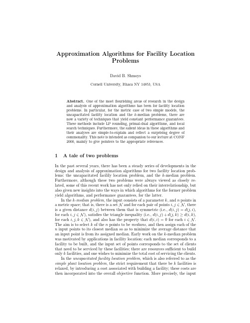
Approximation Algorithms for Facility LocationProblemsDavid B.ShmoysCornell University,Ithaca NY14853,USAAbstract.One of the mostflourishing areas of research in the designand analysis of approximation algorithms has been for facility locationproblems.In particular,for the metric case of two simple models,theuncapacitated facility location and the k-median problems,there arenow a variety of techniques that yield constant performance guarantees.These methods include LP rounding,primal-dual algorithms,and localsearch techniques.Furthermore,the salient ideas in these algorithms andtheir analyses are simple-to-explain and reflect a surprising degree ofcommonality.This note is intended as companion to our lecture at CONF2000,mainly to give pointers to the appropriate references.1A tale of two problemsIn the past several years,there has been a steady series of developments in the design and analysis of approximation algorithms for two facility location prob-lems:the uncapacitated facilily location problem,and the k-median problem. Furthermore,although these two problems were always viewed as closely re-lated,some of this recent work has not only relied on their interrelationship,but also given new insights into the ways in which algorithms for the former problem yield algorithms,and performance guarantees,for the latter.In the k-median problem,the input consists of a parameter k,and n points in a metric space;that is,there is a set N and for each pair of points i,j∈N,there is a given distance d(i,j)between them that is symmetric(i.e.,d(i,j)=d(j,i), for each i,j∈N),satisfies the triangle inequality(i.e.,d(i,j)+d(j,k)≥d(i,k), for each i,j,k∈N),and also has the property that d(i,i)=0for each i∈N. The aim is to select k of the n points to be medians,and then assign each of the n input points to its closest median so as to minimize the average distance that an input point is from its assigned median.Early work on the k-median problem was motivated by applications in facility location:each median corresponds to a facility to be built,and the input set of points corresponds to the set of clients that need to be serviced by these facilities;there are resources sufficient to build only k facilities,and one wishes to minimize the total cost of servicing the clients.In the uncapacitated facility location problem,which is also referred to as the simple plant location problem,the strict requirement that there be k facilities is relaxed,by introducing a cost associated with building a facility;these costs are then incorporated into the overall objective function.More precisely,the inputconsists of two sets of points(which need not be disjoint),the potential facility location points F,and the set of clients C;in this case,we shall let n denote|F∪C|.For each point i∈F,there is a given cost f i that reflects the cost incurred in opening a facility at this location.We wish to decide which facilities to open so as to minimize the total cost for opening them,plus the total cost of servicing each of the clients from its closest open facility.The uncapacitated facility location problem is one of the most well-studied problems in the Operations Research literature,dating back to the work of Balinski[2],Kuehn&Hamburger[11], Manne[14],and Stollsteimer[18,19]in the early60’s.Throughout this paper,aρ-approximation algorithm is a polynomial-time algorithm that alwaysfinds a feasible solution with objective function value within a factor ofρof optimal.Hochbaum[8]showed that the greedy algorithm is an O(log n)-approximation algorithm for this problem,and provided instances to verify that this analysis is asymptotically tight.In fact,this result was shown for the more general setting,in which the input points need not belong to a metric space.Lin&Vitter[12]gave an elegant technique,calledfiltering,for rounding fractional solutions to linear programming relaxations.As one application of this technique for designing approximation algorithms,they gave another O(log n)-approximation algorithm for the uncapacitated facility location problem.Fur-thermore,Lin&Vitter gave an algorithm for the k-median problem thatfinds a solution for which the objective is within a factor of1+ǫof the optimum,but is infeasible since it opens(1+1/ǫ)(ln n+1)k facilities.Both of these results hold for the general setting;that is,the input points need not lie in a metric space. In a companion paper,Lin&Vitter[13]focused attention on the metric case, and showed that for the k-median problem,one canfind a solution of cost no more than2(1+ǫ)times the optimum,while using at most(1+1/ǫ)k facilities.The recent spate of results derive algorithms that can be divided,roughly speaking,into three categories.There are rounding algorithms that rely on lin-ear programming in the same way as the work of Lin&Vitter,in that they first solve the linear relaxation of a natural integer programming formulation of the problem,and then round the optimial LP solution to an integer solution of objective function value no more than factor ofρgreater,thereby yielding aρ-approximation algorithm.The second type of algorithm also relies on the linear programming relaxation,but only in an implicit way;in a primal-dual algorithm,the aim is to simultaneously derive a feasible integer solution for the original problem,as well as a feasible solution to the dual linear program to its linear relaxation.If one can show that the objective function value of the former always is within a factor ofρof the latter,then this also yields aρ-approximation algorithm.Finally,there are local search algorithms,where one maintains a fea-sible solution to the original problem,and then iteratively attempts to make a minor modification(with respect to a prescribed notion of“neighboring”so-lutions)so as to yield a solution of lower cost.Eventually,one obtains a local optimum;that is,a solution of cost no more than that of each of its neighboring solutions.In this case,one must also derive the appropriate structural proper-ties in order to conclude that any locally optimal solution is within a factor of ρof the global optimum.These three classes of algorithms will immediately be blurred;for example,some algorithms will start with an LP rounding phase,but end with a local search phase.One other class of algorithmic techniques should also be briefly mentioned. Arora,Rao,&Raghavan[1]considered these two problems for geometrically-defined metrics.For the2-dimensional Euclidean case of the k-median problem (either when the medians must be selected from among the input points,or when they are allowed to be selected arbitrarily from the entire space)and the uncapacitated facility location problem,they give a randomized polynomial approximation scheme;that is,they give a randomized(1+ǫ)-approximation algorithm,for anyfixedǫ>0.No such schemes are likely to exist for the general metric case:Guha&Khuller[7]proved lower bounds,respectively,of1.463 and1+1/e(based on complexity assumptions,of course)for the uncapacitated facility location problem and k-median problems.2LP rounding algorithmsThefirst approximation algorithm with a constant performance guarantee for the (metric)uncapacitated facility problem was given by Shmoys,Tardos,&Aardal [17].Their algorithm is an LP rounding algorithm;they give a natural extension of the techniques of Lin&Vitter[13]to yield an algorithm with performance guarantee equal to3/(1−e−3)≈3.16.Guha&Khuller[7]observed that one can strengthen the LP relaxation by approximately guessing the proportion of the overall cost incurred by the facilities in the optimal solution,and adding this as a constraint.Since there are only a polynomial number of reasonably-spaced guesses,we can try them all(in polynomial time).Guha&Khuller showed that by adding a local search phase, starting with the solution obtained by rounding the optimum to the“right”LP, one obtains a2.41-approximation algorithm.For their result,the local search is extremely simple;one checks only whether some additional facility can be opened so that the overall cost decreases,and if so,one adds the facility that most decreases the overall cost.The LP rounding approach was further strengthened by Chudak&Shmoys [5,6]who used only the simple LP relaxation(identical to the one used by Lin &Vitter and Shmoys,Tardos,&Aardal),but relied on stronger information about the structure of optimal solutions to the linear programming relaxation to yield a performance guarantee of1+2/e≈1.74.Another crucial ingredient in their approach is that of randomized rounding,which is a technique intro-duced by Raghavan&Thompson[16]in the context of multicommodityflow; in this approach,the fractional values contained in the optimal LP solution are treated as probabilities.Chudak&Shmoys showed how to incorporate the main decomposition results of[17]so as to obtain a variant that might best be called clustered randomized rounding.Chudak&Shmoys also showed that the tech-nique of Guha&Khuller could be applied to their algorithm,and by doing so, one improves the performance guarantee by a microscopic amount.Thefirst constant performance guarantee for the k-median problem also relied an LP rounding approach:Charikar,Guha,Tardos,&Shmoys[4]gave a20/3-approximation algorithm.A wide class of combinatorially-defined lin-ear programs has the property that there exists an optimal solution with the property that each variable is equal to0,1/2,or1;as will be discussed by Hochbaum in another invited talk at this workshop,this property often yields a2–approximation algorithm as a natural corollary.Unfortunately,the linear relaxation used for the k-median problem does not have this property.However, the algorithm of[4]is based on the idea that one can reduce the problem to an input for which there is such an1/2-integral solution,while losing only a con-stant factor,and then subsequently round the1/2-integral solution to an integer one.3Primal-dual algorithmsIn one of the most exciting developments in this area,Jain&Vazirani[9]gave an extremely elegant primal-dual algorithm for the uncapacitated facility location problem;they showed that their approach yields a3-approximation algorithm, and it can be implemented to run in O(n2log n)time.In fact,Jain&Vazirani proved a somewhat stronger performance guarantee;they showed that if we overcharge each facility used in the resulting solution by a factor of3,then the total cost incurred is still within a factor of3of the optimum cost for the unaltered input.In fact,this overcharging is also within a factor of the3of the value of the LP relaxation with the original cost data.Mettu&Plaxton[15]give a variant of this algorithm(which is not explicitly a primal-dual algorithm,but builds substantially on its intuition)that can be implemented to run in O(n2) time,which is linear in the size of the input;this variant does not have the stronger guarantee(but is still a3-approximation algorithm).This stronger performance guarantee for the uncapacitated facility location problem has significant implications for the k-median problem.One natural connection between the two problems works as follows:the facility costs can be viewed as Lagrangean multipliers that enforce the constraint that exactly k facilities are used.Suppose that we start with an instance of the k-median problem,and define an input to the uncapacitated facility location problem by letting C=F=N,and setting the cost of each facility to be a common value φ.Ifφ=0,then clearly all facilities will be opened in the optimal solution, whereas for a sufficiently large value ofφ,only one facility will be opened in the optimal solution.A similar trade-offcurve will be generated by any(reasonable) algorithm for the uncapacitated facility location problem.Jain&Vazirani observed that if their approximation algorithm is used,and φis set so that the number of facilities opened is exactly k,then the resulting solution for the k-median problem has cost within a factor of3of optimal. Unfortunately,the trade-offcurve need not be continuous,and hence it is possiblethat no such value ofφexists.However,if this unlucky event occurs,then one can generate two solutions from essentially equal values ofφ,where one solution has more than k facilities and the other has fewer;Jain&Vazirani show how to combine these two solutions to obtain a new solution with k facilities of cost that is within a factor of6of optimal.Charikar&Guha[3]exploited the fact that these two solutions have a great deal of common structure in order to give a refined analysis;in this way,they derive a4-approximation algorithm for this problem.Mettu&Plaxton[15]also show how to extend their approach to the unca-pacitated facility location problem to obtain an O(n2)-time algorithm for the k-median problem;in fact,their algorithm has the miraculous property that it outputs a single permutation of the input nodes such that,for any k,thefirst k nodes constitute a feasible solution within a constant factor of the optimal k-node solution.Thorup[20]has also given linear-time constant-factor approxi-mation algorithms for the k-median problem;if the metric is defined with respect to a graph with m edges,then he gives a12+o(1)-approximation algorithm that runs in O(m)time.4Local search algorithmsLocal search is one of the most successful approaches to computing,in practice, good solutions to NP-hard optimization problems.Indeed,many of the most visible methods to the general scientific community are variations on this theme; simulated annealing,genetic algorithms,even neural networks can all be viewed as coming from this family of algorithms.In a local search algorithm,more narrowly viewed,one defines a graph on the space of all(feasible)solutions, where two solutions are neighbors if one solution can be obtained from the other by a particular type of modification.One then searches for a node that is locally optimal,that is,whose cost is no more than each of its neighbors,by taking a walk in the graph along progressively improving nodes.Korupolu,Plaxton,&Rajaraman[10]analyzed a local search algorithm in which two nodes are neighbors if exactly one facility is added(or,symmetrically, deleted)in comparing the two solutions,or both one facility is added and one facility is deleted.They show that a local optimum with respect to this neigh-borhood structure has cost within a factor of5of optimal.One further issue needs to be considered in deriving an approximation algorithm:the algorithm needs to run in polynomial time.This can be accomplished in a variety of ways, but typically involves computing a“reasonably good”solution with which to start the search,as well as insisting that a step not merely improve the cost, but improve the cost“significantly”.In this way,they show that,for anyǫ>0, local search can yield a(5+ǫ)-approximation algorithm.Charikar&Guha[3] give a more sophisticated neighborhood structure that yields another simple 3-approximation algorithm.Furthermore,they show that rescaling the relative weight of the facility and the assignment costs leads to a2.415-approximation algorithm based on local search.Finally,they show that all of the ideas abovecan be combined:LP rounding(on multiple LPs augmented as in[7]and aug-mented with a greedy improvement phase),primal-dual algorithms(improved with the rescaling idea),and the improved local search algorithm.In this way, they improve the performance guarantee of1.736due to Chudak&Shmoys to 1.728.This might be the best guarantee known as of this writing,but for these two problems,it seems unlikely to be the last word.References1.S.Arora,P.Raghavan,and S.Rao.Approximation schemes for Euclidean k-medians and related problems.In Proceedings of the30th Annual ACM Symposium on Theory of Computing,pages106–113,1998.2.M.L.Balinksi.Onfinding integer solutions to linear programs.In Proceedingsof the IBM Scientific Computing Symposium on Combinatorial Problems,pages 225–248.IBM,1966.3.M.Charikar and S.Guha.Improved combinatorial algorithms for the facility loca-tion and k-median problems.In Proceedings of the40th Annual IEEE Symposium on Foundations of Computer Science,pages378–388,1999.4.M.Charikar,S.Guha,´E.Tardos,and D.B.Shmoys.A constant-factor approx-imation algorithms for the k-median problem.In Proceedings of the31st Annual ACM Symposium on Theory of Computing,pages1–10,1999.5. F.A.Chudak.Improved approximation algorithms for uncapacitated facility lo-cation.In R.E.Bixby,E.A.Boyd,and R.Z.R´ıos-Mercado,editors,Integer Programming and Combinatorial Optimization,volume1412of Lecture Notes in Computer Science,pages180–194,Berlin,1998.Springer.6. F.A.Chudak and D.B Shmoys.Improved approximation algorithms for theuncapacitated facility location problem.Submitted for publication.7.S.Guha and S.Khuller.Greedy strikes back:Improved facility location algorithms.In Proceedings of the9th Annual ACM-SIAM Symposium on Discrete Algorithms, pages649–657,1998.8. D.S.Hochbaum.Heuristics for thefixed cost median problem.Math.Program-ming,22:148–162,1982.9.K.Jain and V.V.Vazirani.Primal-dual approximation algorithms for metricfacility location and k-median problems.In Proceedings of the40th Annual IEEE Symposium on Foundations of Computer Science,pages2–13,1999.10.M.R.Korupolu,C.G.Plaxton,and R.Rajaraman.Analysis of a local searchheuristic for facility location problems.In Proceedings of the9th Annual ACM-SIAM Symposium on Discrete Algorithms,pages1–10,1998.11. A.A.Kuehn and M.J.Hamburger.A heuristic program for locating warehouses.Management Sci.,9:643–666,1963.12.J.-H.Lin and J.S.Vitter.ǫ-approximations with minimum packing constraintviolation.In Proceedings of the24th Annual ACM Symposium on Theory of Com-puting,pages771–782,1992.13.J.-H.Lin and J.S.Vitter.Approximation algorithms for geometric median prob-rm.Proc.Lett.,44:245–249,1992.14. A.S.Manne.Plant location under economies-of-scale-decentralization and com-putation.Management Sci.,11:213–235,1964.15.R.R.Mettu and C.G.Plaxton.The online median problem.In Proceedings ofthe41st Annual IEEE Symposium on Foundations of Computer Science,2000,to appear.16.P.Raghavan and C.D.Thompson.Randomized rounding:a technique for provablygood algorithms and algorithmic binatorica,7:365–374,1987.17. D.B.Shmoys,´E.Tardos,and K.I.Aardal.Approximation algorithms for facilitylocation problems.In Proceedings of the29th Annual ACM Symposium on Theory of Computing,pages265–274,1997.18.J.F.Stollsteimer.The effect of technical change and output expansion on theoptimum number,size and location of pear marketing facilities in a California pear producing region.PhD thesis,University of California at Berkeley,Berkeley, California,1961.19.J.F.Stollsteimer.A working model for plant numbers and locations.J.FarmEconom.,45:631–645,1963.20.M.Thorup.Quick k-medians.Unpublished manuscript,2000.。
python lineargam参数
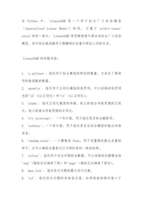
在Python中,`LinearGAM`是一个用于拟合广义线性模型(Generalized Linear Model)的类,它属于`scikit-learn-extra`库的一部分。
`LinearGAM`使用梯度提升算法来拟合广义线性模型,其中线性基函数用于建模响应变量与特征之间的关系。
`LinearGAM`的参数包括:1. `n_splines`: 指定用于拟合模型的特征的数量。
它决定了要使用的基函数的数量。
2. `penalty`: 指定用于正则化模型的惩罚项。
可以选择的惩罚项包括'l2'(L2正则化)和'l1'(L1正则化)。
3. `alpha`: 指定正则化强度的参数。
较大的值会导致更强的正则化,较小的值会导致更弱的正则化。
4. `fit_intercept`: 一个布尔值,用于指定是否拟合截距项。
5. `verbose`: 一个布尔值,用于指定是否在拟合模型时输出详细信息。
6. `random_state`: 一个整数或None,用于设置随机数生成器的种子。
这可以确保在重复运行代码时得到一致的结果。
7. `solver`: 指定用于优化问题的求解器。
可以选择的求解器包括'sag'(随机近似梯度下降)和'saga'(随机近似梯度下降加)。
8. `max_iter`: 指定优化问题的最大迭代次数。
9. `tol`: 指定优化问题的收敛容忍度。
如果残差的绝对值小于tol,则认为模型已收敛。
10. `precompute`: 一个布尔值,用于指定是否使用预计算矩阵来加速计算。
11. `memory`: 用于指定是否使用内存来存储计算矩阵。
可以选择的值包括'auto'(自动选择)和'none'(不使用内存)。
12. `reference`: 指定用于计算目标函数的参考类别。
可以选择的值包括'mean'(使用平均值作为参考类别)和'median'(使用中位数作为参考类别)。
CALF包用户指南说明书
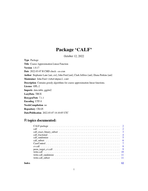
Package‘CALF’October12,2022Type PackageTitle Coarse Approximation Linear FunctionVersion1.0.17Date2022-03-07R CMD check--as-cranAuthor Stephanie Lane[aut,cre],John Ford[aut],Clark Jeffries[aut],Diana Perkins[aut] Maintainer John Ford<****************>Description Contains greedy algorithms for coarse approximation linear functions.License GPL-2Imports data.table,ggplot2LazyData TRUERoxygenNote7.1.1Encoding UTF-8NeedsCompilation noRepository CRANDate/Publication2022-03-0718:10:05UTCR topics documented:CALF-package (2)calf (2)calf_exact_binary_subset (3)calf_fractional (4)calf_randomize (5)calf_subset (6)CaseControl (7)cv.calf (8)perm_target_cv.calf (9)write.calf (10)write.calf_randomize (11)write.calf_subset (11)Index1212calf CALF-package Coarse Approximation Linear FunctionDescriptionForward selection linear regression greedy algorithm.DetailsThe Coarse Approximation Linear Function(CALF)algorithm is a type of forward selection linear regression greedy algorithm.Nonzero weights are restricted to the values+1and-1and their number limited by an input parameter.CALF operates similarly on two different types of samples, binary and nonbinary,with some notable distinctions between the two.All sample data is provided to CALF as a data matrix.A binary sample must contain a distinguishedfirst column with at least one0entries(e.g.controls)and at least one1entry(e.g.cases);at least one other column contains predictor values of some type.A nonbinary sample is similar but must contain afirst column with real dependent(target)values.Columns containing values other that0or1must be normalized,e.g.as z-scores.As its score of differentiation,CALF uses either the Welch t-statistic p-valueor AUC for binary samples and the Pearson correlation for non-binary samples,selected by input parameter.When initiated CALF selects from all predictors(markers)(first in the case of a tie) the one that yields the best score.CALF then checks if the number of selected markers is equal to the limit provided and terminates if so.Otherwise,CALF seeks a second marker,if any,that best improves the score of the sum function generated by adding the newly selected marker to the previous markers with weight+1or weight-1.The process continues until the limit is reached or until no additional marker can be included in the sum to improve the score.By default,for binary samples,CALF assumes control data is designated with a0and case data with a1.It is allowable to use the opposite convention,however the weights in thefinal sum may need to be reversed. Author(s)Stephanie Lane[aut,cre],John Ford[aut],Clark Jeffries[aut],Diana Perkins[aut]Maintainer:John Ford<****************>calf calfDescriptionCoarse Approximation Linear FunctionUsagecalf(data,nMarkers,targetVector,optimize="pval",verbose=FALSE)calf_exact_binary_subset3Argumentsdata Matrix or data frame.First column must contain case/control dummy coded variable(if targetVector="binary").Otherwise,first column must contain realnumber vector corresponding to selection variable(if targetVector="nonbi-nary").All other columns contain relevant markers.nMarkers Maximum number of markers to include in creation of sum.targetVector Indicate"binary"for target vector with two options(e.g.,case/control).Indicate "nonbinary"for target vector with real numbers.optimize Criteria to optimize,"pval"or"auc",(if targetVector="binary")or"corr"(if targetVector="nonbinary").Defaults to"pval".verbose Logical.Indicate TRUE to print activity at each iteration to console.Defaults to FALSE.ValueA data frame containing the chosen markers and their assigned weight(-1or1)The optimal AUC,pval,or correlation for the classification.If targetVector is binary,rocPlot.A plot object from ggplot2for the receiver operating curve. Examplescalf(data=CaseControl,nMarkers=6,targetVector="binary",optimize="pval")calf_exact_binary_subsetcalf_exact_binary_subsetDescriptionRuns Coarse Approximation Linear Function on a random subset of binary data provided,with the ability to precisely control the number of case and control data used.Usagecalf_exact_binary_subset(data,nMarkers,nCase,nControl,times=1,optimize="pval",verbose=FALSE)4calf_fractionalArgumentsdata Matrix or data frame.First column must contain case/control dummy coded variable.nMarkers Maximum number of markers to include in creation of sum.nCase Numeric.A value indicating the number of case data to use.nControl Numeric.A value indicating the number of control data to use.times Numeric.Indicates the number of replications to run with randomization.optimize Criteria to optimize.Indicate"pval"to optimize the p-value corresponding to the t-test distinguishing case and control.Indicate"auc"to optimize the AUC.verbose Logical.Indicate TRUE to print activity at each iteration to console.Defaults to FALSE.ValueA data frame containing the chosen markers and their assigned weight(-1or1)The optimal AUC or pval for the classification.If multiple replications are requested,a data.frame containing all optimized values across all replications is returned.aucHist A histogram of the AUCs across replications,if applicable.Examplescalf_exact_binary_subset(data=CaseControl,nMarkers=6,nCase=5,nControl=8,times=5) calf_fractional calf_fractionalDescriptionRandomly selects from binary input provided to data parameter while ensuring the requested pro-portions of case and control variables are used and runs Coarse Approximation Linear Function.Usagecalf_fractional(data,nMarkers,controlProportion=0.8,caseProportion=0.8,optimize="pval",verbose=FALSE)calf_randomize5 Argumentsdata Matrix or data frame.Must be binary data such that thefirst column must containcase/control dummy coded variable,as function is only approprite for binarydata.nMarkers Maximum number of markers to include in creation of sum.controlProportionProportion of control samples to use,default is.8.caseProportion Proportion of case samples to use,default is.8.optimize Criteria to optimize,"pval"or"auc".Defaults to"pval".verbose Logical.Indicate TRUE to print activity at each iteration to console.Defaults toFALSE.ValueA data frame containing the chosen markers and their assigned weight(-1or1)The optimal AUC or pval for the classification.rocPlot.A plot object from ggplot2for the receiver operating curve.Examplescalf_fractional(data=CaseControl,nMarkers=6,controlProportion=.8,caseProportion=.4) calf_randomize calf_randomizeDescriptionRandomly selects from binary input provided to data parameter and runs Coarse Approximation Linear Function.Usagecalf_randomize(data,nMarkers,targetVector,times=1,optimize="pval",verbose=FALSE)6calf_subsetArgumentsdata Matrix or data frame.Must be binary data such that thefirst column must contain case/control dummy coded variable,as function is only approprite for binarydata.nMarkers Maximum number of markers to include in creation of sum.targetVector Indicate"binary"for target vector with two options(e.g.,case/control).Indicate "nonbinary"for target vector with real numbers.times Numeric.Indicates the number of replications to run with randomization.optimize Criteria to optimize if targetVector="binary."Indicate"pval"to optimize the p-value corresponding to the t-test distinguishing case and control.Indicate"auc"to optimize the AUC.verbose Logical.Indicate TRUE to print activity at each iteration to console.Defaults to FALSE.ValueA data frame containing the chosen markers and their assigned weight(-1or1)The optimal AUC,pval,or correlation for the classification.aucHist A histogram of the AUCs across replications,if applicable.Examplescalf_randomize(data=CaseControl,nMarkers=6,targetVector="binary",times=5) calf_subset calf_subsetDescriptionRuns Coarse Approximation Linear Function on a random subset of the data provided,resulting in the same proportion applied to case and control,when applicable.Usagecalf_subset(data,nMarkers,proportion=0.8,targetVector,times=1,optimize="pval",verbose=FALSE)CaseControl7Argumentsdata Matrix or data frame.First column must contain case/control dummy coded variable(if targetVector="binary").Otherwise,first column must contain realnumber vector corresponding to selection variable(if targetVector="nonbi-nary").All other columns contain relevant markers.nMarkers Maximum number of markers to include in creation of sum.proportion Numeric.A value between0and1indicating the proportion of cases and con-trols to use in analysis(if targetVector="binary").If targetVector="nonbi-nary",this is just a proportion of the full ed to evaluate robustness ofsolution.Defaults to0.8.targetVector Indicate"binary"for target vector with two options(e.g.,case/control).Indicate "nonbinary"for target vector with real numbers.times Numeric.Indicates the number of replications to run with randomization.optimize Criteria to optimize if targetVector="binary."Indicate"pval"to optimize the p-value corresponding to the t-test distinguishing case and control.Indicate"auc"to optimize the AUC.verbose Logical.Indicate TRUE to print activity at each iteration to console.Defaults to FALSE.ValueA data frame containing the chosen markers and their assigned weight(-1or1)The optimal AUC,pval,or correlation for the classification.If multiple replications are requested,a data.frame containing all optimized values across all replications is returned.aucHist A histogram of the AUCs across replications,if applicable.Examplescalf_subset(data=CaseControl,nMarkers=6,targetVector="binary",times=5) CaseControl Example data containing case and control dataDescriptionThis data contains136marker variables for68individuals who are distinguished as case/control. Usagedata(CaseControl)FormatA data frame with136marker variables and68individuals.8cv.calf cv.calf cv.calfDescriptionPerforms cross-validation using CALF data inputUsagecv.calf(data,limit,proportion=0.8,times,targetVector,optimize="pval",outputPath=NULL)Argumentsdata Matrix or data frame.First column must contain case/control dummy coded variable(if targetVector="binary").Otherwise,first column must contain realnumber vector corresponding to selection variable(if targetVector="nonbi-nary").All other columns contain relevant markers.limit Maximum number of markers to include in creation of sum.proportion Numeric.A value between0and1indicating the proportion of cases and con-trols to use in analysis(if targetVector="binary")or proportion of the full sam-ple(if targetVector="nonbinary").Defaults to0.8.times Numeric.Indicates the number of replications to run with randomization.targetVector Indicate"binary"for target vector with two options(e.g.,case/control).Indicate "nonbinary"for target vector with real numbers.optimize Criteria to optimize if targetVector="binary."Indicate"pval"to optimize the p-value corresponding to the t-test distinguishing case and control.Indicate"auc"to optimize the AUC.Defaults to pval.outputPath The path wherefiles are to be written as output,default is NULL meaning no files will be written.When targetVector is"binary"file binary.csv will be outputin the provided path,showing the reults.When targetVector is"nonbinary"filenonbinary.csv will be output in the provided path,showing the results.In thesame path,the kept and unkept variables from the last iteration,will be output,prefixed with the targetVector type"binary"or"nonbinary"followed by Keptand Unkept and suffixed with.csv.Twofiles containing the results from eachrun have List in thefilenames and suffixed with.txt.perm_target_cv.calf9ValueA data frame containing"times"rows of CALF runs where each row represents a run of CALF ona randomized"proportion"of"data".Colunns start with the numer selected for the run,followedby AUC or pval and then all markers from"data".An entry in a marker column signifys a chosen marker for a particular run(a row)and their assigned coarse weight(-1,0,or1).Examples##Not run:cv.calf(data=CaseControl,limit=5,times=100,targetVector= binary )##End(Not run)perm_target_cv.calf perm_target_cv.calfDescriptionPerforms cross-validation using CALF data input and randomizes the target column with each iter-ation of the loop,controlled by’times’.Usageperm_target_cv.calf(data,limit,proportion=0.8,times,targetVector,optimize="pval",outputPath=NULL)Argumentsdata Matrix or data frame.First column must contain case/control dummy coded variable(if targetVector="binary").Otherwise,first column must contain realnumber vector corresponding to selection variable(if targetVector="nonbi-nary").All other columns contain relevant markers.limit Maximum number of markers to include in creation of sum.proportion Numeric.A value between0and1indicating the proportion of cases and con-trols to use in analysis(if targetVector="binary")or proportion of the full sam-ple(if targetVector="nonbinary").Defaults to0.8.times Numeric.Indicates the number of replications to run with randomization.targetVector Indicate"binary"for target vector with two options(e.g.,case/control).Indicate "nonbinary"for target vector with real numbers.10write.calf optimize Criteria to optimize if targetVector="binary."Indicate"pval"to optimize the p-value corresponding to the t-test distinguishing case and control.Indicate"auc"to optimize the AUC.Defaults to pval.outputPath The path wherefiles are to be written as output,default is NULL meaning no files will be written.When targetVector is"binary"file binary.csv will be outputin the provided path,showing the reults.When targetVector is"nonbinary"filenonbinary.csv will be output in the provided path,showing the results.In thesame path,the kept and unkept variables from the last iteration,will be output,prefixed with the targetVector type"binary"or"nonbinary"followed by Keptand Unkept and suffixed with.csv.Twofiles containing the results from eachrun have List in thefilenames and suffixed with.txt.ValueA data frame containing"times"rows of CALF runs where each row represents a run of CALF ona randomized"proportion"of"data".Colunns start with the numer selected for the run,followedby AUC or pval and then all markers from"data".An entry in a marker column signifys a chosen marker for a particular run(a row)and their assigned coarse weight(-1,0,or1).Examples##Not run:perm_target_cv.calf(data=CaseControl,limit=5,times=100,targetVector= binary ) ##End(Not run)write.calf write.calfDescriptionWrites output of the CALF dataframeUsagewrite.calf(x,filename)Argumentsx A CALF data frame.filename The outputfilenamewrite.calf_randomize11 write.calf_randomize write.calf_randomizeDescriptionWrites output of the CALF randomize dataframeUsagewrite.calf_randomize(x,filename)Argumentsx A CALF randomize data frame.filename The outputfilenamewrite.calf_subset write.calf_subsetDescriptionWrites output of the CALF subset dataframeUsagewrite.calf_subset(x,filename)Argumentsx A CALF subset data frame.filename The outputfilenameIndex∗calfCALF-package,2∗datasetsCaseControl,7calf,2CALF-package,2calf_exact_binary_subset,3calf_fractional,4calf_randomize,5calf_subset,6CaseControl,7cv.calf,8perm_target_cv.calf,9write.calf,10write.calf_randomize,11write.calf_subset,1112。
线性代数及离散数学
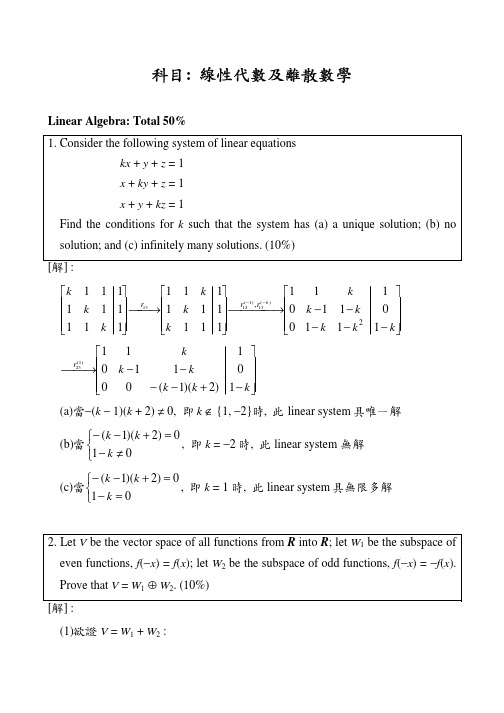
科目: 線性代數及離散數學Linear Algebra: Total 50% 1. Consider the following system of linear equationskx + y + z = 1x + ky + z = 1 x + y + kz = 1Find the conditions for k such that the system has (a) a unique solution; (b) no solution; and (c) infinitely many solutions. (10%)[解] :⎥⎥⎥⎦⎤⎢⎢⎢⎣⎡−−−−−⎯⎯⎯→⎯⎥⎥⎥⎦⎤⎢⎢⎢⎣⎡⎯→⎯⎥⎥⎥⎦⎤⎢⎢⎢⎣⎡−−k k k k k k k k k k k k k r r r 111001101111111111111111111112,)(13)1(1213 ⎥⎥⎥⎦⎤⎢⎢⎢⎣⎡−+−−−−⎯→⎯k k k k k k r 1)2)(1(000110111)1(23 (a)當−(k − 1)(k + 2) ≠ 0, 即k ∉ {1, −2}時, 此linear system 具唯一解(b)當⎩⎨⎧≠−=+−−010)2)(1(k k k , 即k = −2時, 此linear system 無解 (c)當⎩⎨⎧=−=+−−010)2)(1(k k k , 即k = 1時, 此linear system 具無限多解 2. Let V be the vector space of all functions from R into R ; let W 1 be the subspace of even functions, f (−x ) = f (x ); let W 2 be the subspace of odd functions, f (−x ) = −f (x ). Prove that V = W 1 ⊕ W 2. (10%)[解] :(1)欲證V = W 1 + W 2 :∀f ∈ V , 令f x f x f x f x f x f x e o ()(()()),()(()())=+−=−−1212 f x f x f x f x e e ()(()())()−=−+=12, 即f e (x ) ∈ W 1 f x f x f x f x f x f x o o ()(()())(()())()−=−−=−−−=−1212, 即f o (x ) ∈ W 2 而f x f x f x f x f x f x f x e o ()(()())(()())()()=+−+−−=+1212即f = f e + f o ∈ W 1 + W 2所以V = W 1 + W 2(2)欲證W 1 ∩ W 2 = {O } :∀f ∈ W 1 ∩ W 2⇒ f (−x ) = f (x )且f (−x ) = −f (x )⇒ f (x ) = −f (x )⇒ 2f (x ) = 0⇒ f (x ) = 0, ∀x ∈ R所以f = O因此W 1 ∩ W 2 = {0}3. Prove or disprove: Let T be a linear transformation. If vector set {T (v 1), …, T (v n )} is linearly independent, then vector set {v 1, …, v n } is linearly independent. (10%)[解] : True若α1v 1 + ∫ + αn v n = 0⇒ T (α1v 1 + ∫ + αn v n ) = 0⇒ α1T (v 1) + ∫ + αn T (v n ) = 0因為{T (v 1), T (v 2), …, T (v n )}為linearly independent⇒ α1 = ∫ = αn = 0所以{v 1, v 2, …, v n }為linearly independent4. Let T : P 2(R ) → P 2(R ) defined by T (f ) = f (0) + f (1)(x + x 2). Find a basis β such that[T ]β is a diagonal matrix. (10%)[解] :取β0 = {1, x , x 2}為P 2(R )的standard basisT (1) = 1 + 1(x + x 2) = 1 + x + x 2, T (x ) = 0 + 1(x + x 2) = x + x 2T (x 2) = 0 + 1(x + x 2) = x + x 2⎥⎥⎥⎦⎤⎢⎢⎢⎣⎡==⇒111111001][0βT A char A (x ) = det (A − xI ) = −x (x − 1)(x − 2)得A 的eigenvalue 為0, 1, 2⎪⎭⎪⎬⎫⎪⎩⎪⎨⎧⎥⎥⎥⎦⎤⎢⎢⎢⎣⎡−=110)0(span V , ⎪⎭⎪⎬⎫⎪⎩⎪⎨⎧⎥⎥⎥⎦⎤⎢⎢⎢⎣⎡−=111)1(span V , ⎪⎭⎪⎬⎫⎪⎩⎪⎨⎧⎥⎥⎥⎦⎤⎢⎢⎢⎣⎡=110)2(span V 取β = {x − x 2, −1 + x + x 2, x + x 2}, 則⎥⎥⎥⎦⎤⎢⎢⎢⎣⎡==200010000][D T β5. (a) Find an orthonormal basis for the plane x − y − z = 0 in R 3. (b) What point on this plane is closest to (1, 1, 1)? (10%)[解] :(a)令W = {(x , y , z ) | x − y − z = 0} = {(x , y , z ) | z = x − y }= span {v 1 = (1, 0, 1), v 2 = (0, 1, −1)}利用Gram-Schmidt process 對v 1, v 2正交化u 1 = v 1 = (1, 0, 1), <u 1, u 1> = 2) ,1 ,()1 ,0 ,1(21)1 ,1 ,0(,,2121−=−−−=><><−=1111222u u u u v v u , <u 2, u 2>23= 令 ,0 ,(||||2121==111u u w , ) , ,(||||616261−==222u u w則{w 1, w 2}為W 的一組orthonormal basis(b)相當於求v = (1, 1, 1)在W 上的正交投影向量proj W v2211w w v w w v v ><+>=<,,W proj, ,() , ,(62) ,0 ,(23232346162612121=+=− Discrete Mathematics: Total 50% 1. Let a , b , and n be nature numbers.(a) Prove that if a |b , then (2a − 1)|(2b − 1). (5%)(b) Prove that if 2n − 1 is a prime, then n is a prime. (Hint: You may use the result obtained in (a).) (5%)[解] :(a)因為a |b⇒ ∃k ∈ N 使得b = ka2b − 1 = 2ka − 1 = (2a − 1)(2(k −1)a + 2(k −2)a + μ + 2(k −k )a )因為(2(k −1)a + 2(k −2)a + μ+ 2(k −k )a ) ∈ Z⇒ (2a − 1)|(2b − 1)(b)若n 不為prime⇒ ∃a ∈ Z +, 1 < a < n 使得a |n由(a)知(2a − 1)|(2n − 1)因為1 < 2a − 1 < 2n − 1 ⇒ 2n − 1不為primes →←所以n 為prime2. Let m ∈ Z + with m odd. Prove that there exists a positive integer n such that m divides 2n − 1. (10%)[解] :考慮m + 1個正整數21 − 1, 22 − 1, …, 2m − 1, 2m +1 − 1由鴿籠原理知存在二數除以m 具有相同的餘數即∃s , t ∈ Z +, 1 ≤ s < t ≤ m + 1使得(2s − 1)與(2t − 1)具相同的餘數r 令2s − 1 = q 1m + r , 2t − 1 = q 2m + r , 其中0 ≤ r < m⇒ (2t − 1) − (2s − 1) = (q 1m + r ) − (q 2m + r ) = (q 1 − q 2)m⇒ 2t − 2s = (q 1 − q 2)m⇒ m | (2t − 2s )因為2t − 2s = 2s (2t −s − 1)⇒ m | 2s (2t −s − 1)因為m 為奇數, 所以m F 2s⇒ m | (2t −s − 1)取n = t − s ∈ Z +使得m | (2n − 1)3. A connected graph G has 11 vertices and 53 edges. Show that G is Hamiltonian but not Eulerian. (10%)[解] :令G = (V , E ), 其中|V | = 11, |E | = 53, 因為⎟⎟⎠⎞⎜⎜⎝⎛≠2|| ||V E 所以G 不為complete graph因此G 中存在至少二個不相鄰的點∀u , v ∈ V , u , v 不相鄰, 令G 中去掉u , v 得到G' = (V − {u , v }, E') ⇒ |E'| = 53 − (deg (u ) + deg (v ))因為G'具有9個點3629 |'| =⎟⎟⎠⎞⎜⎜⎝⎛≤⇒E 因此, 53 − (deg (u ) + deg (v )) ≤ 36⇒ deg (u ) + deg (v ) ≥ 17 ≥ |V | = 11所以G 含Hamiltonian cycle接著證明G 不含Euler circuit因為K 11含55211=⎟⎟⎠⎞⎜⎜⎝⎛個邊 所以G 相當於由K 11中去掉二個邊的圖因為K 11中每個點的degree 皆為10所以G 中必存在一個點的degree 為9因此G 不含Euler circuit4. Let R be a binary relation. Let S = {(a , b ) | (a , c ) ∈ R and (c , b ) ∈ R for some c }. Show that if R is an equivalence relation, then S is also an equivalence relation.[解] :假設R 及S 皆為A 上的binary relation(1) reflexive :∀a ∈ A , 因為R 具reflexive⇒ (a , a ) ∈ R⇒ (a , a ) ∈ R 且(a , a ) ∈ R⇒ (a , a ) ∈ S(2) symmetric :∀a , b ∈ A , 若(a , b ) ∈ S⇒ ∃c ∈ A 使得(a , c ) ∈ R 且(c , b ) ∈ R因為R 具symmetric⇒ (b , c ) ∈ R 且(c , a ) ∈ R⇒ (b , a ) ∈ S(3) transitive :∀a , b , c ∈ A , 若(a , b ) ∈ S 且(b , c ) ∈ S⇒ ∃c 1, c 2 ∈ A 使得(a , c 1) ∈ R 且(c 1, b ) ∈ R 且(b, c 2) ∈ R 且(c 2, c ) ∈ R因為R具transitive⇒ (a, b) ∈R且(b, c) ∈R⇒ (a, c) ∈S5. Let I = O = {0, 1}. Please construct a state diagram for a finite state machine that recognizes each occurrence of 0110 in a string x∈I∗ (Here overlapping is allowed).[解] :。
sdp松弛和半正定松弛
sdp松弛和半正定松弛
SDP松弛和半正定松弛都是数学优化中常用的方法,主要用于求解凸优化问题。
SDP松弛(Semidefinite Relaxation)是一种将二次规划问题(QP)转化为半正定规划问题(SDP)的方法。
SDP松弛的基本思想是将二次规划问题中的约束条件转化为半正定矩阵形式,将目标函数转化为半正定向量的范数。
这样,SDP松弛将原来的二次规划问题转化为一个半正定规划问题,从而可以使用半正定规划的理论和算法进行求解。
SDP松弛的优点是可以在一定程度上缓解二次规划问题的求解难度,并且可以使用一些高效的求解算法,如半定松弛算法(Semidefinite Relaxation Algorithm)和矩阵分解算法(Matrix Factorization Algorithm)进行求解。
半正定松弛(Semi-Definite Relaxation)是一种将半定规划问题(SDP)转化为半正定规划问题的方法。
半正定松弛的基本思想是将半定规划问题中的约束条件转化为半正定矩阵形式,将目标函数转化为半正定向量的范数。
这样,半正定松弛将原来的半定规划问题转化为一个半正定规划问题,从而可以使用半正定规划的理论和算法进行求解。
半正定松弛的优点是可以在一定程度上缓解半定规划问题的求解难度,并且可以使用一些高效的求解算法,如半定松弛算法和矩阵分解算法
进行求解。
需要注意的是,SDP松弛和半正定松弛都是基于半正定规划的理论和算法进行求解的,因此它们的求解精度和效率都受到半正定规划的限制。
在具体应用时,需要根据问题的特点和求解要求选择合适的方法进行求解。
