Virtual SUSY Threshold Effects and CDF large $E_{T}$ Anomaly
基于感知掩蔽的重构非负矩阵分解单通道语音增强算法
Reconstructed NMF single channel speech enhanceptual masking
Key words: Non-negative Matrix Factorization ( NMF) ; perceived masking; speech enhancement; Speech Presence Probability ( SPP) ; single-channel
Journal of Computer Applications 计算机应用,2019,39( 3) : 894 - 898
ISSN 1001-9081 CODEN JYIIDU
2019-03-10 http: / / www. joca. cn
文章编号: 1001-9081( 2019) 03-0894-05
LI Yansheng, LIU Yuan* , ZHANG Yi
( National Information Accessibility and Service Robot Engineering R&D Center, Chongqing University of Posts and Telecommunications, Chongqing 400065, China)
DOI: 10. 11772 / j. issn. 1001-9081. 2018071489
基于感知掩蔽的重构非负矩阵分解单通道语音增强算法
*
李艳生,刘 园 ,张 毅
( 重庆邮电大学 国家信息无障碍与服务机器人工程研发中心,重庆 400065) ( * 通信作者电子邮箱 1767237325@ qq. com)
非平衡格林函数materials studio

非平衡格林函数materials studio
非平衡格林函数是一个描述物质系统非平衡态的量子力学工具。
它可以用来计算电子在周期性势场中的有限时间存在态,如激发态、极化子和激子等。
非平衡格林函数在材料物理、表面科学、凝聚态物理和量子信息等领域得到广泛应用。
Materials Studio是一个功能强大的材料模拟软件,其中包含一些常用的非平衡格林函数计算工具。
例如,CASTEP可以用来计算非平衡态下的能带结构、光子谱和介电函数;DMol3可以用来计算非平衡态下的电子结构和电子传输特性;VASP和QuantumWise可以用来模拟非平衡态下的电子传输过程和光电特性。
非平衡格林函数的计算需要大量的计算资源和专业知识,对于非专业人士而言比较困难。
因此,在使用Materials Studio进行非平衡格林函数计算前,建议先掌握一定的量子力学和计算化学知识,并进行相关的培训和学习。
基于双重迭代的零样本低照度图像增强

基于双重迭代的零样本低照度图像增强
向森;王应锋;邓慧萍;吴谨;喻莉
【期刊名称】《电子与信息学报》
【年(卷),期】2022(44)10
【摘要】针对低光照条件下拍摄图像质量低下的问题,该文提出一种基于双重迭代的零样本低照度图像增强方法。
其外层迭代通过卷积神经网络估计增强参数,再由内层迭代进行图像增强,增强结果进一步用于计算损失函数并反馈更新外层的参数估计网络,最终通过多轮迭代生成高质量的图像。
在该框架下,还设计了多尺度增强系数估计模块、基于注意力的像素级大气光估计模块,并提出了基于亮度对比度、大气光、颜色均衡以及图像平滑性先验的无监督损失函数。
大量实验结果表明,该方法可有效将低光照图像增强为高质量的清晰图像,其性能优于现有的同类方法。
同时该方法基于零样本学习,不需任何训练数据集,具有良好的普适性。
【总页数】10页(P3379-3388)
【作者】向森;王应锋;邓慧萍;吴谨;喻莉
【作者单位】武汉科技大学信息科学与工程学院;华中科技大学电子信息与通信学院
【正文语种】中文
【中图分类】TN911.73;TP391
【相关文献】
1.基于迭代多尺度引导滤波Retinex的低照度图像增强
2.基于迭代多尺度引导滤波Retinex的低照度图像增强
3.基于MSRCR的自适应低照度图像增强
4.基于深度学习的低照度图像增强
5.基于四元数傅里叶变换的低照度彩色图像增强算法
因版权原因,仅展示原文概要,查看原文内容请购买。
平稳随机振动响应的实数域虚拟激励法
拟响应具有傅里 叶变换 的频谱函数特征 , 以能用实 所 数型哈特莱变换方便地算出虚拟激励 的虚拟响应 。 假定多输人多输出线性时不变稳定 系统的时域零
作 者 郑浩哲 男 , 硕士 , 副教授 , 6 1 4年 9 9 月生
8 6
振 动 与 冲 击
2 1 年第 3 01 0卷
状态单位脉冲响应函数为 h t , () 则频率域复数型系统
r l t n h p b t e n Ha t y t n f r t n a d F u e r n f r t n r a s u o e ctp in e e c n t ce n h ea i s i ew e r e r s mai n o r r t somai e l p e d x i t s w r o s u t d a d t e o l a o o i a o a o r
My()+ ()+ () =n ( ) t t 阵 s ) , ( 的秩数为 r则 用 虚 拟 激励 法计 算 平 稳 随机 振 动 响 应 时 , 需 构 , 只
GridVis-Basic 电力分析仪产品说明书

1Network visualisation software• GridVis ®-Basic (in the scope of supply)3 digital inputs/outputs•Usable as either inputs or outputs•Switch output•Threshold value output •Logic output•Remote via Modbus / ProfibusT emperature measurement •PT100, PT1000, KTY83, KTY84Interfaces •RS485•Ethernet•SNTP •TFTP•BACnet (optional)Networks• T N, T T , IT networks•3 and 4-phase networks•Up to 4 single-phase networksMeasured data memory •256 MB Flash• H armonics up to 40th harmonic •Rotary field components•Distortion factor T HD-U / T HD-I2 analogue inputs • A nalogue, temperature or residual current input (RCM)Residual current measurement BACnet (optional)HomepageAlarm managementMemory 256 MB Ethernet-Modbus gateway2• M easurement, monitoring and checking of electrical characteristics in energy distribution systems • R ecording of load profiles in energy management systems (e.g. ISO 50001)• Acquisition of the energy consumption for cost centre analysis • M easured value transducer for building management systems or PLC (Modbus)• M onitoring of power quality characteristics, e.g. harmonics up to 40th harmonic • R esidual current monitoring (RCM)Areas of applicationMain featuresUniversal meter• O perating current monitoring for general electrical parameters • H igh transparency through a multi-stage and scalable measurement system in the field of energy measurement • A cquisition of events through continuous measurement with 200 ms high resolutionRCM device• C ontinuous monitoring of residual currents (Residual Current Monitor, RCM)• A larming in case a preset threshold fault current reached • N ear-realtime reactions for triggering countermeasures • P ermanent RCM measurement for systems in permanent operation without the opportunity to switch offEnergy measurement device•Continuous acquisition of the energy data and load profiles • E ssential both in relation to energy efficiency and for the safe design of power distribution systemsHarmonics analyser / event recorder• Analysis of individual harmonics for current and voltage •Prevention of production downtimes•Significantly longer service life for equipment • R apid identification and analysis of power quality fluctuations by means of user-friendly tools (GridVis ®)Fig.: UMG 96RM-E with residual current monitoring via measuring inputs I5 / I6Fig.: Event logger: Voltage dip in the low voltage distribution system3Extensive selection of tariffs• 7 tariffs each for effective energy (consumption, delivery and without backstop)• 7 tariffs each for reactive energy (inductive, capacitive and without backstop)•7 tariffs for apparent energy •L1, L2 and L3, for each phaseHighest possible degree of reliability•Continuous leakage current measurement • H istorical data: Long-term monitoring of the residual current allows changes to be identified in good time, e.g. insulation faults•Time characteristics: Recognition of time relationships •Prevention of neutral conductor carryover • R CM threshold values can be optimized for each individual case: Fixed, dynamic and stepped RCM threshold value • M onitoring of the CGP (central ground point) and the sub-distribution panelsAnalysis of fault current events• E vent list with time stamp and values•Presentation of fault currents with characteristic and duration • R eproduction of phase currents during the fault current surge • P resentation of the phase voltages during the fault current surgeAnalysis of the harmonic fault current components•Frequencies of the fault currents (fault type)•Current peaks of the individual frequency components in A and %•Harmonics analysis up to 40th harmonic •Maximum values with real-time bar displayDigital IOs• E xtensive configuration of IOs for intelligent integration, alarmand control tasksFig.: Continuous leakage current measurementFig.: Analysis of fault current eventsFig.: Analysis of the harmonic fault current components4Dimension diagramsAll dimensions in mmSide viewRear viewEthernet (TCP/IP)- / Homepage- / Ethernet-Modbus gateway functionality•Simple integration into the network •More rapid and reliable data transfer •Modern homepage • W orld-wide access to measured values by means of standard web browsers via the device's inbuilt homepage • Access to measurement data via various channels • R eliable saving of measurement data possible over a very long periods of time in the 256 MByte measurement data memory • C onnection of Modbus slave devices via Ethernet-ModbusgatewayFig.: Ethernet-Modbus gateway functionalityMeasuring device homepage• W ebserver on the measuring device, i.e. device's own homepage •Remote operation of the device display via the homepage •Comprehensive measurement data incl. PQ • O nline data directly available via the homepage, historic data optional via the APP measured value monitor, 51.00.246Fig.: Illustration of the online data via the device's inbuilt homepageCut out: 92+0,8 x 92+0,8 mm5Typical connectionDevice overview and technical dataFig.: Connection example residual currentmeasurement and PE monitoringFig.: Connection example with temperature and residual current measurementS2S1S2S2S1S1Digital-Eingänge/Ausgänge UMG 96RM-E (RCM)L1L2L3Spannungsmessung 3456StrommessungVersorgungs-spannung12RS4851617BAB AV e r b r a u c h e r230V/400V 50HzI 41918N282930313233343536Analog-Eingänge13141524V DC K1K2=E t h e r n e t10/100B a s e -TPCK3K4K5==37R J 450-30 mAS2S1I DIFFI 5I 6PT100S1S2S3Gruppe 1Gruppe 2V 1V 2V 3V N N/-L/+2)1)2)2)3)3)3)3)Digital inputs/outputs Power supply voltage Current measurement Measuring voltage Analog inputs L o d s Group 1Group 2Comment:For detailed technical information please refer to the operation manual and the Modbus address list.•= included - = not included *1 Inclusive UL certification.6Fig.: GridVis ®software, configuration menuComment:For detailed technical information please refer to the operation manual and the Modbus address list.• = included - = not included*2 O ptional additional functions with the packages GridVis ®-Professional, GridVis ®-Service and GridVis ®-Ultimate.7Fig.: RCM configuration, e.g. dynamicthreshold value formation, for load-dependent threshold value adaptationFig.: Summation current transformer for the acquisition of residual currents. Wide range with different configurations and sizes allow use in almost all applicationsMeasurement surge voltage Power consumption Overload for 1 sec.Sampling frequency per channel (50 / 60 Hz)Residual current inputAnalogue inputsMeasurement range, residual current input*Digital outputsSwitching voltage Switching current Response timePulse output (energy pulse)Comment:For detailed technical information please refer to the operation manual and the Modbus address list.•= included - = not included*3 E xample of residual current input 30 mA with 600/1 residual current transformer: 600 x 30 mA = 18,000 mA *4A ccurate device dimensions can be found in the operation manual.8Comment:For detailed technical information please refer to the operation manual and the Modbus address list.• = included - = not included。
Robust Principal Component Analysis

∗ John Wright† , Arvind Ganesh† , Shankar Rao† , and Yi Ma†
Department of Electrical Engineering University of Illinois at Urbana-Champaign Visual Computing Group Microsoft Research Asia
Abstract. Principal component analysis is a fundamental operation in computational data analysis, with myriad applications ranging from web search to bioinformatics to computer vision and image analysis. However, its performance and applicability in real scenarios are limited by a lack of robustness to outlying or corrupted observations. This paper considers the idealized “robust principal component analysis” problem of recovering a low rank matrix A from corrupted observations D = A + E . Here, the error entries E can be arbitrarily large (modeling grossly corrupted observations common in visual and bioinformatic data), but are assumed to be sparse. We prove that most matrices A can be efficiently and exactly recovered from most error sign-and-support patterns, by solving a simple convex program. Our result holds even when the rank of A grows nearly proportionally (up to a logarithmic factor) to the dimensionality of the observation space and the number of errors E grows in proportion to the total number of entries in the matrix. A by-product of our analysis is the first proportional growth results for the related but somewhat easier problem of completing a low-rank matrix from a small fraction of its entries. We propose an algorithm based on iterative thresholding that, for large matrices, is significantly faster and more scalable than general-purpose solvers. We give simulations and real-data examples corroborating the theoretical results.
基于改进阈值函数的体震信号平移不变去噪(精)
1
平移不变去噪原理
平移不变去噪首先对带噪信号进行 h 次循
环平移 , 对平移后的信号应用小波阈值法进行处 理, 再对处理后结果进行反向平移并平均, 得到去 噪后的信号 [ 6 ] 对于带噪信号 x ( n ) , n = 1, 2 , , N , 设循环平移算子为 S h , H n = { h | 0 h < n } , Ave 表示平均 , 则 h 次循环平移的平移不变小波 消噪可表示为 T ( x , ( S h) h
第 30 卷第 3 期 2 00 9 年 3 月
东 北 大 学 学 报 ( 自 然 科 学 版 ) Journal of Nort heastern U niversity( Natural Science)
Vol 30, No. 3 Mar. 2 0 0 9
基于改进阈值函数的体震信号平移不变去噪
金晶晶, 王 旭, 吴 雪, 杨 丹
110004) ( 东北大学 信息科学与工程学院 , 辽宁 沈阳
摘
要 : 体震信号微弱 , 受仪器、 环境因素等方面的影响 , 常常含 有大量噪 声 , 研究 一种基于 改进阈值 函
数的平移不变 法用于体震信号的去噪 针对体震信号选择了合适的 小波基 , 说明了 小波分 解后各尺 度上噪 声 方差的估计方法 , 分析了所改进 阈值函数的性能及 特点 , 并给 出了算法的实现步骤 与基于 硬、 软阈值函 数平 移不变法的去噪效果比较 , 基于改进阈值函数平 移不变法去噪后的体震信号波形平滑 , 特征点幅值无衰 减 其 功率谱密度与 原始信号功率谱密度的对 比结果 表明 , 基于改 进阈值 函数的 平移不变 法能够 在去噪 的同时 更 好地保留原始体震信号的特征 关 键 词 : 体震信号 ; 平移不变去噪 ; 噪声方差 ; 改进阈值函数 ; 功率谱密度 中图分类号 : T P 274. 2 文献标识码 : A 文章编号 : 1005 - 3026( 2009) 03 - 0333 - 04
非下采样剪切波域的临近支持向量机去噪方法
非下采样剪切波域的临近支持向量机去噪方法吴昌健;王向阳【摘要】Nonsubsampled Shearlet transform is a kind of excellent multiresolution analysis tool, and it can provide nearly optimal approximation for a piecewise smooth function. Based on nonsubsampled Shearlet transform, an image denoising method using Proximal Classifier with Consistency (PCC) is proposed. Firstly, the noisy image is decomposed into different subbands of frequency and orientation responses using the nonsubsampled Shearlet transform.Secondly, the nonsubsampled Shearlet transformdetail coefficients are divided into two classes (edge-related coefficients and noise-related ones) by PCC training model. Finally, the detail subbands of nonsubsampled Shearlet transform coefficients are denoised by using the adaptable Bayesian threshold. Extensive experimental results demonstrate that the proposed method can obtain better performances in terms of both subjective and objective evaluations than those state-of-the-art denoising techniques. Especially, the proposed method can preserve edges very well while removing noise.%非下采样剪切波( nonsubsampled Shearlet )是一种优秀的多尺度几何分析工具,其不仅可以检测到所有奇异点,而且能够自适应跟踪奇异曲线方向。
Besov空间的阈值收缩和边缘补偿的图像去噪
We io og Wa ur LuZ n l nQan n nS i n e i e g i
Mei l lc0 i aoa。y Suh∞ U i i , nn 10 6,ins C ia dc et nc L brt,,ote 。E r s n e t Naj g20 9 J。gu,hn ) v y i 。 F cl nom t nE gne n n uo ain K n igU i rt c ne n ehooy K n ig6 05 ,u n n C ia ( auyo fr ai n ier ga dA tm t , u mn nv syo i c d Tcnl , u m n 50 1 Y n , hn ) t fI o i o e i fS e a g a
r s e t e y Ex e me t s o t a h d lp r r sw l i e o sn . e p ci l . p r n s h w h tte mo e e fm e l n d n ii g v i o
Ke wo d y rs
I g e osn Be o p c T r s od s rn a e Ed e c mp n ain ma e d n ii g s vs a e h eh l h k g i g o e st o
中指 出用 『 I 1『_来度量数据项 比 更 能捕获噪声。我们 的想法 2
0 引 言
近几 年来 , C nor tC re tSer t 在 o t l 、 uvl 、hal 等变 换域 的 阈值 ue e e 收缩 , 时域 中的变分正则化方法是 图像 去噪的两类主要方法 。 在 阈值收缩是对 变换系数做全局 阈值 切断处 理 , 以考 虑每个 系 难 数的情况 , 损失边缘部分 的系数 , 会 但在平坦 区域去 噪效果非 常 好 。£ 范数空 间扩散 是一个 各 向异性 扩散 , 能够较 好地 保持 边 缘信息 , 但是在平坦 区域 去 噪能力不 强 , 容易 产生方 块效 应 , 范数空 间扩散是一个 各向同性扩散 , 它的平 滑性非常好 , 去噪能 力强 , 是在去 除噪声 的过 程 中模 糊 了边缘 信 息。文献 [ ] 可 1 中
小波去噪阈值的确定和分解层数的确定

代价函数M:
01
常用代价函数:
02
数列中大于给定门限的系数的个数。即预先给定一门限值 ,并计数数列中绝对值大于 的元素的个数。
03
范数。
01
常用代价函数:
02
熵
常用代价函数:
能量对数
“最优树”的搜索方法:
二元树搜索方法:
[thr2,nkeep]=wdcbm(c,l,alpha2);%获得阈值
获取各个高频段的阈值,
阈值选取是根据Birge-Massart准则。
小波去噪阈值的几种方法
[thr,sorh,keepapp]=ddencmp('den','wv',x); xd2=wdencmp('gbl',c,l,wname,level,thr,'h',1);
02
小波包阈值去噪的过程
1 DecompositionFor a given wavelet, compute the wavelet packet decomposition of signal x at level N.(计算信号x在N层小波包分解的系数)2 Computation of the best treeFor a given entropy, compute the optimal wavelet packet tree. Of course, this step is optional. The graphical tools provide a Best Tree button for making this computation quick and easy.(以熵为准则,计算最佳树,当然这一步是可选择的。)3 Thresholding of wavelet packet coefficientsFor each packet (except for the approximation), select a threshold and apply thresholding to coefficients.(对于每一个小波包分解系数,选择阈值并应用于去噪)The graphical tools automatically provide an initial threshold based onbalancing the amount of compression and retained energy. This threshold is.(工具箱会根据压缩量和剩余能量提供一个初始化的阈值,不过仍需要不断测试来选择阈值优化去噪效果)a reasonable first approximation for most cases. However, in general youwill have to refine your threshold by trial and error so as to optimize theresults to fit your particular analysis and design criteria.
virtuallab fusion随机相位的使用

文章标题:探索虚拟实验室Fusion中随机相位的应用序言在现代科学和工程领域,随机相位是一个关键的概念,它在许多不同的领域都有着广泛的应用。
虚拟实验室Fusion作为一个强大的工具,提供了丰富的功能来模拟和研究随机相位的特性及其应用。
本文将深入探讨虚拟实验室Fusion中随机相位的使用,从基础概念到实际应用进行全面评估,并共享个人观点和理解。
一、随机相位的基础概念随机相位是指信号或波在时域或频域上的相位是随机变化的特性。
在信号处理、通信系统、光学和声学等领域,随机相位都扮演着重要的角色。
在虚拟实验室Fusion中,随机相位的模拟和分析需要对其基础概念有清晰的认识,包括随机过程、相关函数、功率谱密度等内容。
二、虚拟实验室Fusion中随机相位的模拟与分析1. 随机相位信号的生成在虚拟实验室Fusion中,可以使用内置的函数或自定义算法来生成具有不同统计特性的随机相位信号,如高斯分布、均匀分布等。
这为研究人员提供了便利的工具,可以模拟各种实际场景中的随机相位信号。
2. 随机相位信号的频谱分析虚拟实验室Fusion提供了丰富的频谱分析工具,可以对生成的随机相位信号进行频谱特性的分析,包括功率谱密度、频谱平坦度等。
通过这些分析,可以更好地理解随机相位信号的频域特性,为实际应用提供参考。
3. 随机相位信号的滤波和处理对于虚拟实验室Fusion的用户来说,随机相位信号的滤波和处理是一个重要的研究方向。
可以通过Fusion提供的滤波器和信号处理算法,对随机相位信号进行去噪、增强等操作,从而提高信号质量和可靠性。
三、随机相位的应用场景与展望随机相位在多个领域都有着重要的应用,如通信系统中的码分多址技术、光学中的相干成像、声学中的噪声抑制等。
虚拟实验室Fusion为研究人员提供了一个强大的评台,可以在这些领域中开展创新性的研究工作,为技术和应用的发展提供有力支持。
结语通过对虚拟实验室Fusion中随机相位的使用进行深入探讨,可以更好地理解随机相位的基础概念和实际应用。
建议收藏 | 肿瘤免疫机制的研究思路
建议收藏 | 肿瘤免疫机制的研究思路背景知识肿瘤是一个复杂的生态系统,其中癌细胞和宿主细胞之间的相互作用影响疾病进展和治疗反应。
除了癌细胞,免疫细胞可以说是实体瘤中最复杂的参与者,其活性范围可以从抗致瘤性到致瘤性。
在肿瘤进展期间,癌细胞会采用多种手段来逃避免疫攻击,例如下调抗原呈现机制或诱导抑制性免疫检查点分子表达。
同时,癌细胞会劫持免疫细胞(如中性粒细胞,巨噬细胞和调节性T细胞(Treg细胞)),来协调免疫抑制性的TME。
这反过来促进免疫逃逸,促进脉管系统和细胞外间质的重塑,并支持癌症进展和治疗抵抗。
因此,异常免疫反应被认为是癌症的标志,并为癌症治疗提供了靶点,最好的例子是免疫检查点阻断(Immune-Checkpoint Blockade,ICB)疗法的成功。
近些年绘制肿瘤细胞结构图和评估单个细胞分子特征的技术快速发展。
这些技术,尤其是单细胞分析、空间转录组分析,为TME的异质性提供了前所未有的见解。
同时,这些技术也揭示了特定癌症类型的内部特征与癌症免疫景观间的异质性。
小编在下文中重点关注遗传变异、表观遗传修饰、细胞信号通路和代谢改变,这些都是塑造癌症免疫景观的癌细胞固有特征[1]。
遗传异常与肿瘤免疫癌症基因组通常会发生多种体细胞改变,例如点突变、DNA片段的插入或缺失、基因组扩增和重排。
这些改变中的一些作为“Driver”,在肿瘤的发生和进展中起作用,而另一些作为“Passenger”,对于癌细胞生长没有影响。
近年来,科研人员将高通量测序技术与高分辨率免疫图谱相结合来分析人类肿瘤,以确定遗传畸变与免疫表型之间的关联,免疫肿瘤学领域从中受益匪浅。
这些研究也发现了新的肿瘤基因与免疫表型相关性。
这一部分的重点往往是影响肿瘤免疫结构和免疫治疗反应的特定癌基因、抑癌基因和DNA损伤机制。
这些遗传畸变会影响免疫格局和肿瘤对免疫治疗的反应。
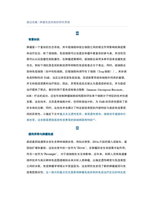
此外,有临床证据已经证实其免疫调节作用(图1)。
图1癌症基因分型与免疫表型的关系MYC是人类肿瘤中最常见的激活癌蛋白之一,也是目前研究最多的一类癌基因。
无边界效应D小波软阈值法去除肉品图像斑点噪声

无边界效应D小波软阈值法去除肉品图像斑点噪声贾渊;彭增起;刘涌;蒋勇【期刊名称】《微计算机信息》【年(卷),期】2011(027)007【摘要】肉品图像中的斑点噪声与肌内脂肪的颜色特征相似,要准确提取肌内脂肪,就必须先对斑点噪声进行滤除.在小波软阈值法滤除SAR图像中的斑点噪声算法基础上,结合肉品图像的特点进行了改进.首先,使用由耿则勋提出的算法,在小波分解时对左右边界进行处理,重构时外推值为0,对离散小波变换的边界效应进行处理,精确重建图像,消除小波变换的边界效应.选择了D8小波,3级分解后,在不同的阈值下进行了实验.结果表明:阈值的选取影响去噪效果,但在所有参数都相同时,改进算法消除边界效应的同时,在斑点指数和方法噪声两个客观评价指标均优于其他几种边界延拓方式,图像失真最小.【总页数】3页(P22-24)【作者】贾渊;彭增起;刘涌;蒋勇【作者单位】621010四川绵阳西南科技大学计算机科学与技术学院;210095 江苏南京南京农业大学食品科技学院;621010四川绵阳西南科技大学计算机科学与技术学院;621010四川绵阳西南科技大学计算机科学与技术学院【正文语种】中文【中图分类】TP274+.3;TS251.5+2【相关文献】1.SAR图像斑点噪声的小波软门限滤除算法 [J], 张俊;柳健2.心脏超声波图像斑点噪声去除方法仿真分析 [J], 裴志松;时兵3.一种改进小波变换相关法去除机载雷达图像斑点噪声的应用 [J], 张宏飞;郑子才;赵凯;陈仁元;王胜源4.基于小波NEIGHSHRINK阈值法滤除SAR斑点噪声 [J], 宁凯;李爱农;陈强;靳华安5.基于3σ准则的小波阈值法在去除红外图像噪声中的应用 [J], 孙婷婷;崔少华因版权原因,仅展示原文概要,查看原文内容请购买。
邻周期采样的数字控制 DC-DC 开关变换器

邻周期采样的数字控制 DC-DC 开关变换器
陈楠;魏廷存;陈笑
【期刊名称】《电机与控制学报》
【年(卷),期】2016(020)007
【摘要】针对高频DC-DC开关变换器,提出了数字控制DC-DC开关变换器的邻周期采样( adjacent cycle sampling ,ACS)控制方法,缓解硬件处理速度与系统瞬态性能之间的矛盾。
依据纹波控制方法,ACS控制算法利用硬件空闲阶段采
样数据,增大环路预留时间,消除占空比的影响。
采用ACS控制算法,推导出适
用于后缘调制降压型DC-DC开关变换器的数字V2控制律和电流控制律,并且研究了次谐振荡现象及其数字斜坡补偿消除方法。
仿真结果表明,在相同的硬件条件,对于负载的瞬间扰动,数字V2控制较数字电流控制具有更快的瞬态响应速度;与现有技术相比,ACS控制方法可有效提高系统的瞬态响应性能。
【总页数】7页(P58-64)
【作者】陈楠;魏廷存;陈笑
【作者单位】西北工业大学计算机学院,陕西西安710072;西北工业大学计算机
学院,陕西西安710072;西北工业大学计算机学院,陕西西安710072
【正文语种】中文
【中图分类】TM46;TP273
【相关文献】
1.数字控制开关变换器瞬态性能的研究 [J], 贺明智;许建平;郝瑞祥
2.基于FPGA的DC/DC开关变换器的数字控制器 [J], 贺明智;许建平;胡晓明
3.数字控制系统中的采样周期和数字滤波 [J], 金孚安
4.一种新颖的DC-DC开关变换器数字控制方法 [J], 冷朝霞;刘健;刘庆丰;王华民
5.数字控制系统采样周期对控制质量的影响 [J], 周平;黎亚元
因版权原因,仅展示原文概要,查看原文内容请购买。
体全息存储记录通道噪声模型的研究与设计

体全息存储记录通道噪声模型的研究与设计
吴非;刘朝斌;谢长生;陈端容
【期刊名称】《计算机科学》
【年(卷),期】2006(033)004
【摘要】体全息存储系统具有存储容量大、数据传输率快、存储时间短以及能快速进行图像或图形匹配和内容相关寻址操作的潜力,极有可能成为下一代大容量数据存储方法.但是体全息存储记录通道中复杂的噪声来源一直是妨碍体全息存储技术实用化的主要问题之一.本文将分析体全息存储通道中存在的各种噪声来源,并提出记录通道噪声的物理模型,为设计噪声的抑制方法奠定理论基础.
【总页数】4页(P13-15,35)
【作者】吴非;刘朝斌;谢长生;陈端容
【作者单位】华中科技大学计算机学院外存储国家重点实验室,武汉,430074;大连海事大学计算机科学与技术学院,大连,116026;华中科技大学计算机学院外存储国家重点实验室,武汉,430074;华中科技大学计算机学院外存储国家重点实验室,武汉,430074
【正文语种】中文
【中图分类】TP3
【相关文献】
1.基于聚合物全息光盘的体全息存储演示仪 [J], 刘鸿鹏;王维波
2.一个体全息存储高速数据通道的设计 [J], 刘洋;谢长生;吴非;胡迪青;罗东健
3.体全息光存储高速存储通道设计中的关键技术研究 [J], 倪永军;余本海;罗东建
4.新一代无纸记录仪——具有多输入通道、大存储容量、长时间记录特性 [J],
5.厚度对光聚物高密度全息存储记录参量的影响 [J], 黄明举;姚华文;陈仲裕;侯立松;干福熹
因版权原因,仅展示原文概要,查看原文内容请购买。
lammps vacf 计算声子态密度

lammps vacf 计算声子态密度声子态密度是量子力学中的一个重要概念,它把量子结构和电子特性连接在一起,对研究原子阱、原子结构以及电子谱都有重要作用。
它可以用来描述材料中电子的行为,使得研究者可以获得有关电子行为的准确信息。
计算声子态密度的方法通常包括周期性可能法(PP)、经典原子轨道(CAO)、格林函数(GF)和虚拟散射(VS)等。
然而,这些方法有时难以获得准确的结果,或者需要大量的计算时间。
mps vacf是一种新的、可靠的计算声子态密度的方法,它包含了一种称为极化调和谱(VACF)的算法,能够提供精确的声子态密度。
该算法基于一种独特的内插技术,可以显著减少计算时间,这使得该算法比其他常见的计算声子态密度的方法更加有效。
此外,通过使用VACF计算声子态密度,研究者可以更好地理解电子的特性和行为,因为这种方法可以更好地描述电子行为。
mps vacf计算声子态密度的优点不仅限于它减少计算时间和提供准确的结果。
它还有助于更好地研究和理解材料中电子的特性和行为,因为它提供了有关电子态密度的准确信息。
因此,研究者可以使用这些信息来研究材料中电子态密度所反映的物理特性,例如热力学性质、电子结构和能带结构等。
此外,还有许多软件可以用来实施mps vacf,如VASP,QuantumEsspresso,LAMMPS等,它们可以根据用户的需求提供有效的分子动力学计算结果。
因此,研究者可以根据实验条件来选择最合适的软件,从而获得有关声子态密度的准确信息。
综上所述,mps vacf是一种有效的计算声子态密度的方法,它可以减少计算时间,提供准确的结果,同时也可以更好地理解材料中电子的特性和行为。
虽然它仍然有一些局限性,但是它仍然是一种有用的工具,可以提供有关电子行为的准确信息。
从理论上讲,mps vacf是一种新颖、有效的计算声子态密度的方法,它可以显著减少计算时间,提供准确的结果,并且可以更好地理解材料中的电子特性和行为。
基于异质性预矫正的小波域SAR图像去斑

基于异质性预矫正的小波域SAR图像去斑
侯建华;陈稳;刘欣达;陈少波
【期刊名称】《计算机应用研究》
【年(卷),期】2016(33)7
【摘要】真实SAR图像在去斑过程中易存在过平滑现象,针对此问题提出了一种对图像预矫正后再进行去斑处理的方法.对含斑图像作小波分解,以多尺度局部变差系数作为异质性测度,提出一种基于该测度的自适应预矫正函数,将小波子带划分为四类区域,对各区域采取不同的预处理策略;在此基础上对预矫正图像采用常规的小波域去斑算法.对真实SAR图像去斑的实验表明,该方法在抑制相干斑和保持图像细节方面均有较显著的改善.这种预矫正过程简单、实用,并且可以和多种常规的去斑算法相结合,具有一定的推广和应用价值.
【总页数】4页(P2224-2227)
【作者】侯建华;陈稳;刘欣达;陈少波
【作者单位】中南民族大学智能无线通信湖北省重点实验室,武汉430074;中南民族大学智能无线通信湖北省重点实验室,武汉430074;中南民族大学智能无线通信湖北省重点实验室,武汉430074;中南民族大学智能无线通信湖北省重点实验室,武汉430074
【正文语种】中文
【中图分类】TP391.41
【相关文献】
1.基于小波域隐马尔可夫混合模型的SAR图像降斑算法 [J], 吴艳;王霞;廖桂生
2.基于异质性分类的小波域SAR图像去斑 [J], 侯建华;陈稳;刘欣达;陈少波
3.基于自相关函数建模的小波域SAR图像去斑方法 [J], 王文;芮国胜;王晓东
4.一种基于复小波域的SAR图像相干斑抑制算法 [J], 肖竹;钟桦;易克初
5.基于预筛选的改进的SAR图像PPB去斑 [J], 胡开洋;耿伯英
因版权原因,仅展示原文概要,查看原文内容请购买。
自由呼吸THRIVE序列动态增强MRI联合DWI在孤立性肺结节良恶性鉴别诊断的应用价值
自由呼吸THRIVE序列动态增强MRI联合DWI在孤立性肺结节良恶性鉴别诊断的应用价值姚平竺;夏炎;周小媚;黎加识【期刊名称】《哈尔滨医药》【年(卷),期】2024(44)1【摘要】目的对孤立性肺结节患者予以自由呼吸THRIVE序列动态增强MRI联合DWI检查,以观察该检查方法对于结节性质鉴别诊断中的价值。
方法在进行孤立性肺结节检查的患者中随机选择100例进行本次研究。
所有患者均予以MRI检查。
以病理结果为最终检查结果,将纳入研究的100例患者分为良性组和恶性组,比较不同序列信号强度、DCE-MRI定量参数、ADC值在不同性质的肺结节中的差异,则分析有差异的相关参数对于鉴别诊断的效能。
结果100例孤立性肺结节患者经过病理检查,最终确诊71例为恶性,占比71%,29例为良性,占比为29%。
根据结节性质将患者进行分组,结果发现良性组和恶性组患者MRI常规信号T1-VIBE、T2-VIBE、T2-HASTE结果差异无统计学意义(P>0.05);对两组患者进行DWI和DCE-MRI定量检测,结果发现良性组患者Ktrans、Kep水平均低于恶性组,ADC水平高于恶性组,差异均有统计学意义(P<0.05),两组患者维生素E水平差异无统计学意义(P>0.05);对Ktrans、Kep、ADC、Ktrans+Kep+ADC诊断孤立性肺结节良恶性的效能使用ROC曲线进行分析,结果发现Ktrans、Kep、ADC对于孤立性肺结节的诊断均具有较好的诊断效能,其中Kep的AUC最高危0.778,但是三者联合应用的AUC面积和约登指数均超过各指标单独应用,分别为0.829和0.659。
结论自由呼吸THRIVE序列动态增强MRI联合DWI能够显著增加孤立性肺结节良恶性鉴别的诊断效能,具有重要的临床应用价值。
【总页数】3页(P62-64)【作者】姚平竺;夏炎;周小媚;黎加识【作者单位】东莞市茶山医院【正文语种】中文【中图分类】R563.9【相关文献】1.动态增强MRI灌注差异在良恶性孤立性肺结节鉴别诊断中的应用价值2.CT灌注成像联合动态增强扫描检查在鉴别诊断孤立性肺结节良、恶性中的应用价值3.128层CT多征象分析联合动态增强扫描对孤立性肺结节良、恶性鉴别诊断的价值4.自由呼吸Star-VIBE序列动态增强MRI联合DWI在孤立性肺结节诊断中的应用因版权原因,仅展示原文概要,查看原文内容请购买。
基于自适应动态限幅的水下图像增强算法改进

基于自适应动态限幅的水下图像增强算法改进于君霞【摘要】针对水下特殊的水体环境,考虑到水体对光的吸收作用以光的散射,得到的水下图像普遍存在颜色失真和对比度下降的现象.本文对此提出了一种自适动态限幅直方图均衡化算法.直方图均衡化算法实际上是一个直方图重新分布和像素重新映射的过程.而动态限幅直方图均衡化算法就是直方图重新分布和像素重新映射,动态划分灰度的映射区间,区间独立进行均衡化.首先求出RGB各个通道的均值然后进行对比判断,根据均值的大小来决定是一端拉伸还是两端拉伸,拉伸的过程也是线性拉伸,然后转换到HSI颜色空间进行饱和度和亮度拉伸,最终得到视觉效果较好的水下图像[1].【期刊名称】《西部皮革》【年(卷),期】2017(039)022【总页数】2页(P30,32)【关键词】水下光场;动态限幅;RGB;灰度直方图【作者】于君霞【作者单位】中国海洋大学, 山东青岛 266100【正文语种】中文【中图分类】TN911.73由于我国近海沿岸的水质比较浑浊,再加上水介质的衰减作用,使光子在水中的传播受到很大程度的能量吸收抑或传播方向上散射,尤其是散射效应使得目标物的反射光子或照明路径中的后向散射光子会在成像界面中产生很多的影响噪点,降低目标物的对比度,甚至淹没图像。
我们必须要对图像进行增强或复原,才能对水下的真实情况和信息进行了解,以便于更好的研究和利用图像对水下的勘测和分析。
所以,图像增强和图像处理对于水下资源的探索就显得尤其重要且不可或缺。
由于后向水下图像会产生噪声,对比度低,并且会产生颜色失真[2]。
因此我们要对划分的每个小区域都必须使用对比度限幅。
但是,传统直方图均衡化处理会导致灰度图像出现过度增强和光晕等退化效应,影响了灰度图像处理前后的均值稳定性。
针对传统直方图峰值剪切的弊端,本文采用自适应动态限幅处理技术。
首先对图像分块处理(一般采用8*8),以免处理后的彩色图像会出现局部颜色不均匀的情况,并且对每个小区域都必须使用对比度限幅。
- 1、下载文档前请自行甄别文档内容的完整性,平台不提供额外的编辑、内容补充、找答案等附加服务。
- 2、"仅部分预览"的文档,不可在线预览部分如存在完整性等问题,可反馈申请退款(可完整预览的文档不适用该条件!)。
- 3、如文档侵犯您的权益,请联系客服反馈,我们会尽快为您处理(人工客服工作时间:9:00-18:30)。
a rXiv:h ep-ph/961503v25Fe b1997KEK-TH-477YUMS-96-27SNUTP-96-110(February 1,2008)Virtual SUSY Threshold Effects and CDF large E T Anomaly C.S.Kim 1,2∗and S.Alam 2†1:Department of Physics,Yonsei University,Seoul 120-749,Korea 2:Theory Group,KEK,Tsukuba,Ibaraki 305,Japan Abstract Recent CDF data of the inclusive jet cross section shows threshold-like struc-tured deviation,around transverse momentum E T (j )≈200∼350GeV.If this data is real,not just some statistical fluctuation,is it possible to interpret the anomaly in terms of virtual SUSY effects?The purpose of this note is to address this question.However,we find that virtual SUSY loop interference effects [near the threshold]are too small to explain the CDF data.Our main conclusion seems to be on the right track if we assume that the recent globalanalysis of improved parton distributions by Lai et al.is correct.I.INTRODUCTIONThe CDF[1]and D0[2]collaborations at Tevatron Collider have recently reported√data for the inclusive jet cross section in p¯p collisions atThere are basically two logical possibilities for explanations of the CDF data on inclu-sive jet production cross sections:(i)the parton distribution functions determined at low Q2region may not be accurate enough to be applicable to the high ET region with ET>200GeV,or(ii)there are some new physics around the electroweak scale.We give a brief reviewof these two possibilities in the following.Let usfirst consider thefirst possibility.According to the CDF collaboration[1]“the excess of data over theory at high ETremains for CTEQ2M,CTEQ2ML,GRV94,MRSA′, and MRSG parton distribution”.The variations in QCD predictions represented a survey of then-available distributions.They do not represent the uncertainties associated with data used in deriving the PDF’s.Inclusion of these new data in a globalfit with those from otherexperiments may yield a consistent set of PDF’s which will accommodate the high-ETexcess within the scope of QCD.Glover et al.,[3]conclude that“it is unlikely that the difference between the CDF inclusive jet cross section data and standard NLO QCD prediction can be attributed to a deficiency in our knowledge of parton distributions”.More precisely Glover et al.[3]find from their global analysis that it is impossible tofit both the CDF data forET>200GeV and Deep Inelastic Scattering[DIS]data for x>0.3.However,as notedin[8]the interpretation of large ETjet cross sections inherits uncertainties from the non-perturbative parton distribution and fragmentation functions.It has recently been reported [4]that the apparent discrepancy between CDF data and theory may be explained by the uncertainties resulting from the non-perturbative parton distribution,in particular in the gluon distribution at large x.These authors have also performed NLO QCD global analysisincluding the CDF data and conclude that high ETcan be explained in terms of a modified gluon PDF.However,we note that Lai et al.[4]use more parameters to describe the input gluon distribution than is usually done,whereas Glover et al.[3]assume that the gluon distribution has a canonical behavior[i.e.goes as(1−x)n]at large x.3It is also tempting to look for a possible explanation for the CDF data in terms of new physics.The CDF group[1]have reported on a model of presence of quark substructure[5]. They have compared their data to leading order QCD calculation including compositeness and have used MRSD0′parton distribution.Theyfind a good agreement between data and>200GeV,for a substructure scale ofΛC=1.6TeV.the compositeness model,for ETYet another possibility is that jet measurements at hadron colliders may be sensitive to quantum corrections due to virtual SUSY particles[6–9].The purpose of this note is to concentrate on this scenario.The layout and of this paper is as follows.In next section we discuss our calculation of the SUSY virtual threshold effects.Thefinal section contains discussions and conclusions of our numerical results.II.VIRTUAL SUSY THRESHOLD EFFECTSWe consider the SUSY one loop corrections to the process dσ(p¯p→2jets).As is well-known,the2jets production cross section in proton anti-proton collisions is found by weighing the expressions for differential cross section of the subprocess,dˆσij≡dˆσ(ij→2final partons),by the parton distribution functions,and integrating over the parton vari-ables,i.e.dσ(p¯p→2jets)= i,j 10dx1 10dx2[f i/p(x1,Q2)f j/¯p(x2,Q2)]dˆσij(αs,ˆs,ˆt,ˆu).(1)Here dˆσij represents the subprocess cross section at c.m.energy square ofˆs=x1x2s,where √dα2s(µ).(2)2πIn the SM,b3is given by2b3=11−n f−2−13authors of Ref.[8],working in the context of MSSM,consider at around the threshold energy scale the virtual one-loop corrections to the parton-level subprocesses q¯q→q¯q,q¯q→q′¯q′, qq′→qq′,q¯q→gg and qg→qg,which are expected to dominate the large E T cross sections at the Tevatron energy[i.e.(b),(c)].The purpose of this note is to give our results of incorporating the one-loop radiative corrections into the running ofαs,the dressing-up of the parton distribution functions,and finally convoluting the relevant subprocess cross sections with the SUSY dressed-up PDF’s [i.e.(a),(b),(c),(d)].In the hadron colliders,like the Tevatron,what is measured is p¯p cross section,and not the individual subprocesses cross sections.So in order to determine the effect of subprocesses on the ETcross section one must perform a convolution of the cross section of each subprocess with the corresponding PDF’s[i.e.(d)].Wefind that in the process of convolution with the PDF’s,the“dips and peaks”in the various subprocesses[8] are much reduced.We note that,also as pointed out in[8],one should take into account sparticles effects on the parton structure functions at energies sufficiently far above the threshold,and can ignore this effect around the threshold region[i.e.(a)].We test the validity of this statement andfind it to be true from our numerical work,as will be shown in Fig.2.We have considered the combined evolution equations forαs,q vd4πα2s(Q2),(5)d2πP NS0⊗q NS(x,Q2).(6)The second equation becomes,with the definition of p NS=xq NS,d3π 1 xdzπ[1+4The increase ofαs(Q2)results in the decrease of the PDF compared to the SM when we make the evolution.The qualitative reason is rather simple:strongerαs(Q2)as Q2increases imply that the gluon radiation from the initial quarks are enhanced,and the PDF evolution yields the larger gluon or sea-quark densities at the smaller x region,and therefore the valence quark distribution q v(x,Q2)decreases at large x,asαs(Q2)increases,and vice versa.We recall that for large x the valence contribution dominates(e.g.q v·q v:q v·g:g·g∼0.65:0.3:0.05at x∼0.3at Tevatron energies),we ignored the SUSY evolution of sea-quark or gluon for large Eof CDF.It turns out,as shown in Fig.2and claimed in Ref.[8],the PDF with sparticle Teffects at around the threshold region deviates much less than0.1%from its SM predictions, which justifies our assumption.And we can even totally ignore the SUSY corrections to PDF[i.e.(a)]all together for investigations below or around the threshold region.III.NUMERICAL RESULTS AND CONCLUSIONSFor our numerical calculation,we implement various lower bounds on squarks and gluinos depending on parameters in the MSSM.For example,D0group[10]searched for the events with large missing Ewith three or more jets,observed no such events above theTlevel expected in the SM.This puts some limits on the squark and gluino masses assuming the short-lived gluinos:m˜g>144GeV for m˜q=∞,(8)or m˜g=m˜q>212GeV.(9) CDF group is currently analyzing their data,with their preliminary data being similar to the D0results with slight increase in sparticles’mass bound.In the subsequent numerical7analysis,we choose three sets of(m˜g,m˜q),which we shall refer to as Case I,II and III, respectively,(m˜g,m˜q)=(220GeV,220GeV),(150GeV,∞),(150GeV,150GeV).(10)The Case III is only of academic interest if the limit given in Eq.(9)is valid in reality.We turn now to our numerical result.The solid curve in Fig.1represents the one-loop evolution ofαs(µ)versus the renormalization scaleµfor the SM,assuming a top-quark mass of175GeV,andΛQCD=0.2GeV.The long-dashed curve represents the results for the MSSM with thefive squarks and gluinos being degenerate with a common mass of220GeV [we shall refer to this as Case I].As can be seen from Fig.1,Case I starts to deviate from the SM results atµ=440GeV,as expected.The deviation in the value ofαs away from the SM is maximum[for our range ofµ]atµ=700GeV and roughly on the order of5%.This value is to be compared to the12%reported in[6].The dotted curve in Fig.1describes our result for the MSSM with gluino mass of150GeV,and the squarks are assumed to be decoupled,we shall refer to this as Case II.Case II starts to be different from the SM at µ=300GeV.The maximum deviation for Case II occurs at around700GeV,where it also approaches the curve for Case I.The deviation from the SM of the one-loop evolution for the parton distribution func-tion[(MSSM−SMthus resulting in a reduction in u v.Turning to Case II,we see from Fig.2that it deviates from the SM at Q=300GeV,reaching a maximum value of only−0.1%at700GeV.Fig.3exhibits our results for[(MSSM−SMdpT j ]versus pT jfor both Cases I and III[CaseIII refers the MSSM with thefive squarks and gluinos being degenerate with a common mass of150GeV,i.e.the last set in Eq.(10)].A rapidity cut of0.7is used[|η|<0.7].A maximum difference of−1%from the SM is found for the both Cases.The question that naturally arises is,that why the“dips and peaks”[which are at the level of5%–6%[8]]at the parton level,are reduced.There are two factors contributing to the reduction in the“dips and peaks”in the process of going from the parton to the process level.Part of this reduction comes from the process of convolution of the various subprocesses with PDF’s[as already remarked to in the previous section].The other piece of this reduction in“dips and peaks”by going from subprocess to process level is due to t-channel“dilution”effect.This can be shown by simply not including the t-channel subprocesses’contribution.When this is done [see Fig.4a and4b]reduction in the“peaks and dips”is not so large.In Fig.4(a)we exhibit our results for[(MSSM−SMdpT j ]versus pT jfor both Cases Iand III,but this time only including the subprocesses q¯q−→q′¯q′and q¯q−→gg.These two are the subprocesses with the prominent threshold structures from vacuum polarization interferences through s-channel exchange diagrams.A rapidity cut of0.7is used[|η|<0.7]. The deviation from the SM for Case I varies between2%to−4%,whereas as in Case II the variation is similar size to Case I at different energy scales related to the SUSY threshold effects.In Fig.4(b)we exhibit our results for[(MSSM−SMdM jj]versus M jj for both the Cases I and III,including the subprocesses q¯q−→q′¯q′and q¯q−→gg.The percentage variation is almost the same as in Fig.4(a).Near the virtual(or direct)SUSY threshold,the Coulomb interactions between the gluinos[or squarks]with a very small velocity v=depending on the parameterαs/v,rather than onαs.The result of summing up the Coulomb exchanges reduces to multiplying the Coulomb factorαs/v[11],which gives a wide resonance structure around Q≈2m˜g for the short-lived gluino pairs.If the life time of gluino is long enough,then narrow bound states of gluino pair may appear near the threshold region.Since the properties on gluino pair bound states are not known and largely model dependent,we can guess only qualitative nature of the threshold region,Q≈2m˜g(or Q≈2m˜q),as shown in Fig.3and4.In summary,in the MSSM the Edistributions does not differ very much from those ofTthe SM except for the possible threshold effects(∼1%)through loop corrections.In actual experiments,the jet resolution will in general smear out any narrow resonance structures (which may be the case for the long-lived gluinos),leading to broad resonance structure,and therefore it looks impossible to detect SUSY particles through this kind of indirect virtual threshold effect.As is previously explained,it has been reported[4]that the apparent discrepancy between CDF data and theory may be explained by the uncertainties resulting from the non-perturbative parton distribution,in particular in the gluon distribution.Our main conclusion seems to be on the right track in view of this global analysis of parton distribution function.ACKNOWLEDGEMENTSThe authors would like to thank E.L.Berger,M.Drees,P.Ko,Jake Lee and J.W.Qui for useful suggestions and helpful comments.The work of CSK was supported in part by the KOSEF,Project No.951-0207-008-2,in part by CTP of SNU,in part by the BSRI Program, Project No.BSRI-97-2425,and in part by the COE Fellowship from Japanese Ministry of Education,Science and Culture.The work of SA is supported by COE fellowship of the Japanese Ministry of Education,Science and Culture.10REFERENCES[1]CDF Collaboration:F.Abe et al.,Phys.Rev.Lett.77(1996)438.[2]D0Collaboration:G.Blazey,talk given at Recontre de Moriond,(March1996).[3]E.W.N.Glover et al.,Phys.Lett.B381(1996)353.[4]i et al.,hep-ph/9606399.[5]E.Eichten et al.,Phys.Rev.Lett.50(1983)811.[6]V.Barger et al.,Phys.Lett.B383(1996)178.[7]P.Kraus and F.Wilczek,Phys.Lett.B382(1996)262.[8]J.Ellis and D.Ross,Phys.Lett.B383(1996)187.[9]S.Alam et al.,Phys.Rev.D55(1997)1.[10]D0Collaboration:S.Abachi et al.,Phys.Rev.Lett.75(1995)618.[11]V.S.Fadin et al.,Yad.Fiz.48(1988)309.FIGURESFig.1The one-loop evolution ofαs(µ)versusµis given for SM[solid line]and SUSY cases. Fig.2Percentage deviation from the SM due to SUSY contribution of PDF of the valence quark versus factorization scale Q for typical momentum fraction x=0.3.Fig.3Deviation from the SM due to SUSY contribution to dσdpT j versus pT j,when only thesubprocesses q¯q→q′¯q′,and q¯q→gg are included.11Fig.4b Deviation from the SM due to SUSY contribution to dσ。