ANSYS WorkBench 13.0从入门到精通
Ansys_Workbench详解教程全解 共72页

编辑目标
用户可以对给定的目标进行复制、 粘贴、剪切等常规操作。使用Edit菜单 中的各项命令。
2019/7/15
19
视图显示
视图的显示主要在View菜单中进行控制。 1、图形窗口
Shade Exterior and Edges:轮廓线显示 Wireframe:线框显示 Ruler:显示标尺 Legend:显示图例 Triad:显示坐标图示
2019/7/15
30
定义材料属性
4、在线性静力结构分析当中,材料属性只需要定义杨氏模量以及泊松比。
– 假如有任何惯性载荷,密度是必须要定义的;模态分析中同样需要定义材 料密度。
2019/7/15
31
3 网格控制
目的:实现几何模型
原则:整体网格控制
有限元模型的转化 局部网格细化
2019/7/15
有限元法的基本思想对弹性区域离散化将单元内任一节点位移通过函数表达位移函数建立单元方程进行单元集成在节点上加外载荷力引入位移边界条件进行求解求解得到节点位移根据弹性力学公式得到单元应变应力有限元法的基本步骤根据弹性力学公式计算单元应变应力
ANSYS Workbench12.0 基础培训讲义
(内部共享)
方法二:单击开始菜单,
选择程序命令;
从Ansys程序组
中选择
AnsysWorkbench程序。
启动该软件后,出现一模块选择对话框。
2019/7/15
10
操作界面介绍
2019/7/15
11
菜单
常用的几个菜单项为:
—“File > Save” 用来保存数据库文件:.dsdb —“File > Clean” 用来删除数据库中的网格或结果 —“Edit > Select All” 用来选取窗口中当前的所有实体 —“Units” 用来改变单位 —“Tools >options” 用来定制或设置选项
ANSYS13.0官方入门操作指南(英文打印版)
Table of Contents2.1. Entering a Processor2.2. Exiting from a Processor or ANSYS2.2.1. Stopping the Input of a File2.3. The ANSYS Database2.3.1. Defining or Deleting Database Items2.3.2. Saving the Database2.3.3. Restoring Database Contents2.3.4. Using the Session Editor to Modify the Database2.3.5. Clearing the Database2.4. ANSYS Program Files2.4.1. ANSYS File Types2.4.2. ANSYS File Sizes2.4.3. The Jobname.LOG File2.5. Communicating With the ANSYS Program2.5.1. Communicating Via the Graphical User Interface (GUI)2.5.2. Communicating Via Commands2.5.3. Command Defaults2.5.4. Abbreviations2.5.5. Command Macro Files3.1. Starting an ANSYS Session from the Command Level3.2. The Mechanical APDL Product Launcher3.2.1. Starting an ANSYS Session from the Start Menu/Launcher3.2.2. Launcher Menu Options3.3. Interactive Mode3.3.1. Executing the ANSYS or DISPLAY Programs from Windows Explorer 3.4. Batch Mode3.4.1. Starting a Batch Job from the Command Line3.5. Choosing an ANSYS Product via Command Line3.6. Setting Preferences with the start130.ans File3.6.1. The start130.ans File4.1. GUI Controls4.1.1. A Dialog Box and Its Components4.2. Activating the GUI4.3. Layout of the GUI4.3.1. The Utility Menu4.3.2. The Standard Toolbar4.3.3. Command Input Options4.3.4. The ANSYS Toolbar4.3.5. The Main Menu4.3.6. The Graphics Window4.3.7. The Output Window4.3.8. Creating, Modifying and Positioning Toolbars5.1. Locational and Retrieval Picking5.2. Query Picking5.2.1. The Model Query Picker5.2.2. The Results Query Picker6.1. The Configuration File6.2. Splitting Files Across File Partitions6.3. Customizing the GUI6.3.1. Changing the GUI Layout6.3.2. Changing Colors and Fonts6.3.3. Changing the GUI Components Shown at Start-Up6.3.4. Changing the Mouse and Keyboard Focus6.3.5. Changing the Menu Hierarchy and Dialog Boxes Using UIDL6.3.6. Creating Dialog Boxes Using Tcl/Tk6.4. ANSYS Neutral File Format6.4.1. Neutral File Specification6.4.2. AUX15 Commands to Read Geometry Into the ANSYS database6.4.3. A Sample ANSYS Neutral File Input Listing7.1. Using the Session Log File7.2. Using the Database Command Log7.3. Using a Command Log File as InputRelease 13.0 - © 2010 SAS IP, Inc. All rights reserved.Chapter 1: Introducing ANSYSANSYS finite element analysis software enables engineers to perform the following tasks:●Build computer models or transfer CAD models of structures, products, components, orsystems.●Apply operating loads or other design performance conditions.●Study physical responses, such as stress levels, temperature distributions, or electromagneticfields.●Optimize a design early in the development process to reduce production costs.●Do prototype testing in environments where it otherwise would be undesirable or impossible(for example, biomedical applications).The ANSYS program has a comprehensive graphical user interface (GUI) that gives users easy, interactive access to program functions, commands, documentation, and reference material. An intuitive menu system helps users navigate through the ANSYS program. Users can input data using a mouse, a keyboard, or a combination of both.This manual provides basic instructions for operating the ANSYS program: starting and stopping the product, using and customizing its GUI, using the online help system, etc. For other information about using ANSYS, see the following documents:●For general instructions on performing finite element analyses for any engineering discipline,see the Basic Analysis Guide, the Modeling and Meshing Guide, and the Advanced Analysis Techniques Guide.●For information about performing specific types of analysis (thermal, structural, etc.), see theapplicable Analysis Guide.●For examples of analyses, see the Mechanical APDL Tutorials and Verification Manual.●For reference information about ANSYS commands, elements, and theory, see the CommandReference, Element Reference, and Theory Reference for the Mechanical APDL and Mechanical Applications.Chapter 2: The ANSYS EnvironmentThe ANSYS program is organized into two basic levels:●Begin level●Processor (or Routine) levelThe Begin level acts as a gateway into and out of the program. It is also used for certain global program controls such as changing the jobname, clearing (zeroing out) the database, and copying binary files. When you first enter the program, you are at the Begin level.At the Processor level, several processors are available. Each processor is a set of functions that perform a specific analysis task. For example, the general preprocessor (PREP7) is where you build the model, the solution processor (SOLUTION) is where you apply loads and obtain the solution, and the general postprocessor (POST1) is where you evaluate the results of a solution. An additional postprocessor, POST26, enables you to evaluate solution results at specific points in the model as a function of time.The following environment topics are available:●Entering a Processor●Exiting from a Processor or ANSYS●The ANSYS Database●ANSYS Program Files●Communicating With the ANSYS Program2.1. Entering a ProcessorIn general, you enter a processor by selecting it from the ANSYS Main Menu in the Graphical User Interface (GUI). For example, choosing Main Menu > Preprocessor takes you into PREP7. Alternatively, you can use a command to enter a processor (the format is /name, where name is the name of the processor). Table 2.1: Processors (Routines) Available in ANSYS lists each processor, its function, and the command to enter it.2.2. Exiting from a Processor or ANSYSTo return to the Begin level from a processor, pick Main Menu > Finish or issue the FINISH (or /QUIT) command. You can move from one processor to another without returning to the Begin level. Simply pick the processor you want to enter, or issue the appropriate command.To leave the ANSYS program (and return to the system level), pick Utility Menu > File > Exit or use the /E XIT command to display the Exit from ANSYS dialog box. By default, the program saves the model and loads portions of the database automatically and writes them to the database file, Jobname.DB. If a backup of the current database file already exists, ANSYS writes it to Jobname.DBB. Options in the dialog box (and on the /EXIT command) allow you to save other portions of the database or to quit without saving.2.2.1. Stopping the Input of a FileYou can also stop the processing of an ANSYS file as it is being input. Most files of more than a few lines will display the ANSYS Process Status window at the top of the screen. If you want to terminate the input of a file, select the STOP button on the ANSYS Process Status window. ANSYS itself does not stop when you select the STOP button. Stopping file input is useful if you inadvertently input a binary file.To input a new file, select Utility Menu > File > Clear & Start New to clear the current file from memory, then select a file to input. If you want to return to processing the original file, select Utility Menu > File > Read Input from... and select the name of the file, the line number or label to resume from, and select the OK button. See the /INPUT command for more information on resuming a file input process.2.3. The ANSYS DatabaseIn one large database, the ANSYS program stores all input data (model dimensions, material properties, load data, etc.) and results data (displacements, stresses, temperatures, etc.) in an organized fashion. The main advantage of the database is that you can list, display, modify, or delete any specific data item quickly and easily.No matter which processor you are in, you are working with the same database. This gives you basic access to the model and loads portions of the database from anywhere in the program. "Basic access" means the ability to select, list, or display an item.The following database topics are available:●Defining or Deleting Database Items●Saving the Database●Restoring Database Contents●Using the Session Editor to Modify the Database●Clearing the Database2.3.1. Defining or Deleting Database ItemsTo define items, or to delete items from the database, you must be in the appropriate processor. For example, you can define nodes, elements, and other geometry only in PREP7, the general preprocessor. You can specify and apply loads in either the PREP7 or the SOLUTION processor, and you can declare optimization variables only in OPT (the design optimization processor). However, you can select geometry items, list them, or display them from anywhere in the program, including the Begin level.2.3.2. Saving the DatabaseBecause the database contains all your input data, you should frequently save copies of it to a file. To do this, pick Utility Menu > File > Save as Jobname.DB or issue the SAVE command. Either choice writes the database to the file Jobname.DB. If you use the SAVE command, you have the option to save:●the model data only●the model and solution data●the model, solution and preprocessing dataTo specify a different file name, pick Utility Menu > File > Save as or use the appropriate fields on the SAVE command. Any save operation first writes a backup of the current database file (if the database already exists) to Jobname.DBB. If a Jobname.DBB file already exists, the new backup file overwrites it. For a static or transient structural analysis, the file Jobname.RDB (a copy of the database) will be automatically saved at the first substep of the first load step.2.3.3. Restoring Database ContentsTo restore data from the database file, pick Utility Menu > File > Resume Jobname.DB or issue the RESUME command. This reads the file Jobname.DB. To specify a different file name, pick Utility Menu > File > Resume from or use the appropriate fields on the RESUME command.You can save or resume the database from anywhere in the ANSYS program, including the Begin level.A resume operation replaces the data currently in memory with the data in the named database file. Using the save and resume operations together is useful when you want to "test" a function or command. When you do a multiframe restart, ANTYPE,,REST automatically resumes the .RDB file for the current job.2.3.4. Using the Session Editor to Modify the DatabaseDuring an analysis, you may want to modify or delete commands entered since your last SAVE or RESUME. You can access the session editor by issuing the UNDO command, or by choosing Main Menu > Session Editor. The session editor display is shown below.Figure 2.1 The Session EditorUse this dialog for displaying and editing the string of operations performed since your last SAVE or RESUME command. You can modify command parameters, delete whole sections of text, and even save a portion of the command string to a separate file.You can access the following file operations from the session editor dialog:●OK: Enters the series of operations displayed in the window below. You will use this option toinput the command string after you have modified it.●Save: Saves the command string displayed in the window below to a separate file. ANSYSnames the file Jobnam000.cmds, with each subsequent save operation incrementing the filename by one digit. You can use the /INPUT command to reenter the saved file.●Cancel: Dismisses this window and returns to your analysis.●Help: Displays the command reference for the UNDO command.The Session Editor is available in interactive (GUI) mode only. If no SAVE or RESUME command has been issued during your analysis, all commands from your current session will be executed, including your start130.ans file, if present.2.3.5. Clearing the DatabaseWhile building a model, sometimes you may want to clear out the database contents and start over. To do so, choose Utility Menu > File > Clear & Start New or issue the /CLEAR command. Either method clears (zeros out) the database stored in memory. Clearing the database has the same effect as leaving and reentering the ANSYS program, but does not require you to exit.2.4. ANSYS Program FilesThe ANSYS program writes and reads many files for data storage and retrieval. File names follow this pattern:Name.ExtName defaults to the jobname, which you can specify while entering the ANSYS program or by choosing Utility Menu > File > Change Jobname (equivalent to issuing the /FILNAME command). The default jobname is FILE (or file).Ext is a unique, two- to four-character ANSYS identifier that identifies the contents of the file. For example, Jobname.DB is the database file, Jobname.EMA T is the element matrix file, and Jobname.GRPH is the neutral graphics file. Some systems (such as PCs) truncate the extension to three characters. Also, the extension may be in lowercase, depending on the system.The following program file topics are available:●ANSYS File Types●ANSYS File Sizes●The Jobname.LOG File2.4.1. ANSYS File TypesTable 2.2: ANSYS File Types and Formats lists the main ANSYS file types and their formats. For more information about files, see File Management and Files in the Basic Analysis Guide.On the following ANSYS commands, you can specify the name and path of the file to be written:/ASSIGN*LIST/COPY/OUTPUT*CREATE/PSEARCH/DELETE/RENAME/INPUTIn such cases, the filename can contain up to 248 characters, including the directory name, and the extension can contain up to eight characters. If the file name uses more than 248 characters, including the directory, you must use a soft link on UNIX/Linux systems.ANSYS can process blanks in file or directory names, so blank spaces are allowed in ANSYS object names. Be aware that many UNIX/Linux commands do not support object names with spaces. When an object has a blank space in its name, always enclose the name in a pair of single quotes.On UNIX/Linux systems, all directory names except for /(root) should end with a slash (/). For example, to run the ANSYS program using an input file called vm1.dat, which resides in the directory /ansys_inc/v130/ansys/data/verif, use the following commands:ansys130/inp,vm1,dat, /ansys_inc/v130/ansys/data/verif/On Windows systems, you must use back slashes (\) instead of slashes in directory names. For example, on a Windows system, the directory path shown in the UNIX example above looks like this:/inp,vm1,dat, Program Files\Ansys Inc\V130\ANSYS\data\verif\2.4.2. ANSYS File SizesThe maximum size of an ANSYS file depends on the file system on the hard drive partition being used. Most computer systems now handle very large files without any need for the automatic file splitting option that is provided in ANSYS. The FAT32 file system is occasionally still used on some Windows and Linux systems and has a file size limitation of 4 GB. We recommend converting any FAT32 hard drives to a file system that can support much larger files (e.g., for Windows, we recommend converting to the NTFS file system). If you are running a problem that will create an ANSYS file over 4 GB on a system using a FAT32 hard drive, then you can use the /CONFIG,FSPLIT command to set the maximum ANSYS file size to any value under 4 GB.2.4.3. The Jobname.LOG FileThe Jobname.LOG file (also called the session log) is especially important, because it provides a complete log of your ANSYS session. The file opens immediately when you enter the ANSYS program, and it records all commands you execute, whether you execute those commands via GUI paths or type them in directly. You can read the Jobname.LOG file, view it while in ANSYS, edit it, and input it later.The ANSYS program always appends log data to the log file instead of overwriting it. If you change the jobname while in an ANSYS session, the log file name does not change to the new jobname. For more information about Jobname.LOG, see Using the ANSYS Session and Command Logs.2.5. Communicating With the ANSYS ProgramThe easiest way to communicate with the ANSYS program is by using the ANSYS menu system, called the Graphical User Interface (GUI).2.5.1. Communicating Via the Graphical User Interface (GUI)The GUI consists of windows, menus, dialog boxes, and other components that allow you to enter input data and execute ANSYS functions simply by picking buttons with a mouse or typing in responses to prompts. All users, both beginner and advanced, should use the GUI for interactive ANSYS work. See Using the ANSYS GUI for an extensive discussion of how to use the GUI. The rest of this section describes other topics related to communication with ANSYS commands, abbreviations, etc.2.5.2. Communicating Via CommandsCommands are the instructions that direct the ANSYS program. ANSYS has more than 1200 commands, each designed for a specific function. Most commands are associated with specific (one or more) processors, and work only with that processor or those processors.To use a function, you can either type in the appropriate command or access that function from the GUI (which internally issues the appropriate command). The Command Reference describes all ANSYS commands in detail, and also tells you whether each command has an equivalent GUI path. (A few commands do not.)ANSYS commands have a specific format. A typical command consists of a command name in the first field, usually followed by a comma and several more fields (containing arguments). A comma separatesYou can abbreviate command names to their first four characters (except as noted in the Command Reference). For example, FINISH, FINIS, and FINI all have the same meaning. Some "commands" (such as ADAPT and RACE) are actually macros. You must enter macro names in their entirety.Note:If you are not sure whether an instruction is a command or a macro, see the Command Reference.Commands that begin with a slash ( / ) usually perform general program control tasks, such as entry to routines, file management, and graphics controls. Commands that begin with a star ( * ) are part of the ANSYS Parametric Design Language (APDL). See the ANSYS Parametric Design Language Guide for details.Command arguments may take a number or an alphanumeric label, depending on their purpose. In the F command example described previously, NODE and VALUE are numeric arguments, but Lab is an alphanumeric argument. In this and other ANSYS manuals, numeric arguments appear in all uppercase italic letters (as in NODE and VALUE), and alphanumeric arguments appear in initial uppercase italic format (as in Lab). Some commands (for example, /PREP7, /POST1, FINISH, etc.) have no arguments, so the entire command consists of just the command name.Some general rules and guidelines for commands are listed below:●When you enter commands, the arguments do not have to be in specific columns.●You can use successive commas to skip arguments. When you do so, ANSYS uses defaultvalues for the omitted arguments (as discussed in the individual command descriptions).●You can string together multiple commands on the same line by using the $ character as thedelimiter for each command. (For restrictions on use of the $ delimiter, see the Command Reference.)●The maximum number of characters allowed per line is 640, including commas, blank spaces,$ delimiters, and any other special characters.Note: Other software programs and printers may wrap text to the next line or truncate the text after a certain character.●Real number values input to integer data fields will be rounded to the nearest integer. Theabsolute value of integer data must fall between zero and 2,000,000,000.●The acceptable range of values for real data is +/-1.0E+200 to +/-1.0E-200. No exponent canexceed +200 or be less than -200. The program accepts real numbers in integer fields, but rounds them to the nearest integer. You can specify a real number using a decimal point (such as 327.58) or an exponent (such as 3.2758E2). The E (or D) character, used to indicate an exponent, may be in upper or lower case. This limit applies to all ANSYS input commands, regardless of platform.Even though all ANSYS input must be within the allowed range, all numeric operations, including parametric operations, can produce numbers to machine precision, which may exceed the ANSYS input range.●ANSYS interprets numbers entered for Angle arguments as degrees. Note that there arefunctions in ANSYS that could use radians if the *AFUN command had been used.●The following special characters are not allowed in alphanumeric arguments:! @ # $ % ^ & * ( ) _ - += | \ { } [ ] " ' / < > ~ `●Exceptions are filename and directory arguments, where some of these characters may berequired to specify system-dependent pathnames. However, using special characters in filename and directory arguments could result in ANSYS or the operating system misreading the argument. We strongly recommend that you limit filename and directory arguments to A-Z, a-z, 0-9, -, _, and spaces. Any text prefaced by an exclamation mark (!) is treated as a comment.●Avoid using tabs (to line up comments, for instance) or other control (CTRL) sequences. Theyusually generate device-dependent characters that the program cannot recognize.●If you are a longtime ANSYS user, avoid using commands that have been removed from thecurrently documented command set. Such commands are obsolete and may cause difficulties.2.5.3. Command DefaultsTo minimize the amount of data input, most commands have defaults. There are two types of defaults: command default and argument default.A command default is the specification assumed when a command is not issued. For example, if you do not issue the /FILNAME command, the jobname defaults to FILE (or whatever jobname was specified when you entered the ANSYS program).An argument default is the value assumed for a command argument if the argument is not specified. For example, if you issue the command N,10 (defining node 10 with the X, Y, Z coordinate arguments left blank), the node is defined at the origin; that is, X, Y, and Z default to zero. Numeric arguments (such as X, Y, Z) default to zero except as noted in the Command Reference. The command descriptions usually explain defaults for other arguments.Note:The defaults for some commands and their arguments differ depending on which ANSYS product is using the commands. The "Product Restrictions" section of the descriptions of the affected commands clearly documents such cases. If you plan to use your input file in more than one ANSYS product, youshould explicitly specify commands or command argument values, rather than letting them default. Otherwise, behavior in the other ANSYS product may be different from what you expect.2.5.4. AbbreviationsIf you use a command or a GUI function frequently, you can rename it or abbreviate it to a string of up to eight alphanumeric characters using one of the following:Command(s): *ABBRGUI: Utility Menu > Macro > Edit Abbreviations Utility Menu > MenuCtrls > Edit ToolbarFor example, the following command defines ISO as an abbreviation for the command /VIEW,,1,1,1 (which specifies isometric view for subsequent graphics displays):*ABBR,ISO,/VIEW,,1,1,1Keep the following rules and guidelines in mind when creating abbreviations:●The abbreviation must begin with a letter and should not have any spaces.●If an abbreviation that you set matches an ANSYS command, the abbreviation overrides thecommand. Therefore, use caution in choosing abbreviation names.●You can abbreviate up to 60 characters, and up to 100 abbreviations are allowed per ANSYSsession.In the GUI, abbreviations appear as push buttons on the Toolbar, which you can execute with a quick click of the mouse. For details, see the section on using the toolbar in Using the ANSYS GUI .2.5.5. Command Macro FilesYou can record a frequently used sequence of ANSYS commands in a macro file, thus creating a personalized ANSYS command. If you enter a command name that ANSYS does not recognize, it searches for a macro file by that name (with an extension of .MAC or .mac). If the file exists, ANSYS executes it.On UNIX/Linux and Windows systems, the ANSYS program searches for macro files in the following order:●ANSYS looks first in the ANSYS APDL directory.●It then looks at the directories that have been defined for the environmental variableANSYS_MACROLIB. You can set up the ANSYS_MACROLIB variable after the installation of ANSYS software and before the program is started.On UNIX/Linux, the structure for ANSYS_MACROLIB is:dir1/:dir2/:dir3/On Windows, the structure is:c:\dir1\;d:\dir2\;e:\dir3The letter to the left of the colon indicates the drive where the directory is stored.Enter up to 2048 characters for the entire string. Dir1 is searched first, followed by dir2, dir3, etc. These files provide customization at both the site and user levels.●Next, on UNIX/Linux systems, ANSYS looks in /PSEARCH or in the login directory. OnWindows systems, it looks in /PSEARCH or in the home directory.●Finally, ANSYS looks in the current or working directory.ANSYS searches for both upper and lower case macro file names in each search directory, except /apdl on UNIX/Linux systems. If both exist in the search directory, the upper case file is used. Only upper case is used in the /apdl directory on UNIX/Linux systems.The ANSYS installation media provide many ANSYS macro files that reside in the /apdl subdirectory. If you cannot use any of the ANSYS-provided macro files, contact your system administrator.To access any macro, you simply enter its file name. For instance, to access the LSSOLVE.MAC file, you enter LSSOLVE. You can also access macros you created via the Utility Menu > Macro > Execute Macr o menu path. However, this menu path will not work for any macros containing function granules (such as a call to a dialog box) or picking commands. Macros with these functions must be accessed by entering the macro name in the Input Window.Specifying File Names in WindowsIn the Windows environment, some devices/ports have specific names, such as PRN, COM1, COM2, LPT1, LPT2, and CON. The device/port names resemble files in that they can be opened, read from, written to, and closed. Entering the names of these devices/ports in ANSYS, however, causes unpredictable behavior, including system freezes or fatal error conditions. Therefore, do not issue PC device/port names as commands.Configuring Search Paths on Windows Systems1. In the Control Panel, click on the System Icon.2. On Windows XP systems, click on My Computer on the Start Menu. Under System Tasks,select View System Information. Select the Advanced Tab. Click on the Environment Variables button. Click New under System Variable. Enter the value of ANSYS_MACROLIB for the variable name. Enter<drive > :\<dir > \;<drive > :\<dir2 > \;<drive > :\<dir3 > \;for the variable value. Click OK.3. On Windows 2000 systems, select the Advanced tab. Click on the Environment Variablesbutton. Click on the New button under System Variables. Enter the value of ANSYS_MACROLIB for the variable name. Enter<drive > :\<dir > \;<drive > :\<dir2 > \;<drive > :\<dir3 > \;for the variable value. Click on the OK button.。
有限元分析—ANSYS13 0从入门到实战

有限元分析—ANSYS13 0从入门到实战- 1 - 本书是针对现有的ANSYS图书实例单一工程背景不强重操作少原理的现状特以ANSYS13.0为平台撰写的一部从入门到精通的实用自学和提高教程。
全面介绍有限元分析的理论基础、有限元分析流程、实体建模、网格划分、施加载荷、求解、通用后处理、时间历程后处理、静力学分析、结构动力学分析、结构非线性分析、复合材料分析断裂力学分析热力学分析、边坡稳定性分析、界面开裂分析、衬垫连接分析、齿轮分析、转子动力学分析、焊接过程、优化设计、拓扑优化、疲劳分析、自适应网格分析和可靠性分析等内容。
围绕ANSYS软件的功能讲解书中给出了大量具有工程背景的实例详细讲解热门问题如冲压回弹分析J积分计算、螺栓衬垫法兰盘连接分析齿轮动态接触分析焊接残余热应力分析等实例。
本书具有以下特点语言通俗易懂逻辑严密深入浅出。
切实从读者学习和使用的实际出发安排章节顺序和内容。
图文并茂。
讲述过程中结合大量分析实例力求易于理解并方便学习和实践过程中的使用。
本书配套光盘提供了共22个实例的视频教程和ANSYS实例文件。
本书不仅适合高等学校理工类高年级本科生或研究生学习ANSYS 13.0有限元分析软件的教材还可供从事结构分析的工程技术人员参考使用同时书中提供的大量实例也可供高级用户参考。
第1章绪论 1.1有限单元法基本概念有限单元法的基本思想是将连续的求解区域离散为一组有限个、且按一定方式相互联结在一起的单元的组合体。
由于单元能按不同的联结方式进行组合且单元本身又可以有不同形状因此可以对复杂的模型进行求解。
有限单元法作为数值分析方法的另一个重要特点是利用在每一个单元内假设的近似函数来分片地表示全求解域上待求的未知场函数。
单元内的近似函数通常由未知场函数或其导数在单元的各个节点的数值和其插值函数来表达。
这样一来一个问题的有限元分析中未知场函数或及其导数在各个节点上的数值就成为新的未知量从而使一个连续的无限自由度间题变成离散的有限自由度问题。
Ansys_workbench学习系列教程01_认识Workbench
14
Ansys Workbench 系列学习教程
第一部分的悬臂梁理论计算结果如下: 力矩=100Nm
回路阻值仿真计算案例
弯矩: 100NM 弯曲应力(Y 方向):
解析与仿真计算对比
项目
挠度 弯矩 弯曲应力
计算值
20.2 100 127.4
仿真值
21.3 100 127.6
有限元求解满足实际工误差要求
Ansys_workbench 学习系列教程 01
认识 Ansys_WorkBench
目录
一.一个简单的仿真案例 二.理论分析与仿真对比 三.如何学好有限元仿真计算
Ansys Workbench 系列学习教程
一
回路阻值仿真计算案例
一个简单的仿真案例
0 引言
在这一章里,你将初步认识 workbench,如何利 用 workbench 完成一个材料力学中提及的悬臂 梁的力学分析。 技能点:
创建线体(Line)模型 第一步:点击 modelling 图标,选择 concept>line from sketching 第二步:点击选择已建立的 Sketch1 图标; 第三步:点击 Apply 图标; 第四步:点击 Generate 图标,生成线模型
5
Ansys Workbench 系列学习教程
回路阻值仿真计算案例
至此,完成了分析
几何模型的建立。 6.双击项目流程简图中的 model 图标 ,进入分析界面。
7.为 Line 体赋材料属性 第一步:点击选择 line body; 第二步:点击选择 Assignment 中的箭头,打开工程材料库; 第三步:点击选择 Structural Steel 完成材料赋值;
ANSYS从入门到精通[完整版总结]
![ANSYS从入门到精通[完整版总结]](https://img.taocdn.com/s3/m/ea3d4bee951ea76e58fafab069dc5022aaea468b.png)
1、ANSYS分析的目的 (5)2、有限元法基本构成和主要功能 (5)2.1 ANSYS有限元的基本构成: (5)2.2 ANSYS软件的组成 (5)3、 ANSYS界面介绍 (6)3.1 ANSYS功能菜单(Utility Menu) (6)3.1.1 文件菜单(File) (6)3.1.2 选择菜单(Select) (6)3.1.3 列表显示菜单(List) (7)3.1.4 图形显示菜单(Plot) (7)3.1.5 图形显示控制菜单(PlotCtrls) (7)3.1.6 工作平面菜单(WorkPlane) (8)3.1.7 参数菜单(Parameters) (8)3.1.8 宏命令菜单(Macro) (9)3.1.9 菜单控制菜单(MenuCtrls) (9)3.2 输入窗口(Input Window) (9)3.3 工具栏(Toolbar) (9)3.4 主菜单(Main Menu) (10)3.5 图形窗口(Graphic Window) (10)3.6 图形显示控制按钮 (10)3.7 提示栏 (11)3.8 隐藏的输出窗口 (11)4、ANSYS文件系统 (11)5、ANSYS典型分析过程 (12)5.1 ANSYS分析前的准备工作 (12)5.2 通过前处理器Preprocessor建立模型 (12)5.3 通过求解器Solution加载求解 (12)5.4 通过后处理器General Postproc或TimeHist Postproc查看分析结果 (12)6、 ANSYS中的坐标系 (12)6.1 ANSYS中坐标系的分类: (13)6.2 总体坐标系 (13)6.3 局部坐标系 (13)6.4 显示坐标系 (14)6.5 节点坐标系 (14)6.6 单元坐标系 (14)6.7 结果坐标系 (14)7、工作平面 (14)8、网格划分 (14)8.1 概述 (15)8.2 设置单元属性表 (15)8.3 网格划分前分配单元属性 (15)8.3.1 直接给实体模型图元分配单元属性 (15)8.3.2 分配默认属性 (15)8.4 网格划分控制 (15)8.4.1 网格划分工具 (16)9、施加荷载 (22)9.1 荷载分类 (22)9.2 荷载步、子步、平衡迭代 (23)9.3 时间的作用【TIME】 (23)9.4 加载方式 (24)9.5 荷载步选项 (24)9.6 创建多荷载步 (27)9.7 载荷的施加 (28)10 求解过程 (30)10.1 概述 (30)10.2 求解器 (30)10.3 求解方式 (32)10.3.1 一般求解 (32)10.3.2 多荷载步求解 (33)10.3.2.1 多重求解法 (33)10.3.2.2 荷载步文件法 (33)10.3.3 重新启动分析 (34)10.4 求解控制 (34)10.5 可能出现的问题 (36)11、结果后处理 (36)11.1 后处理器 (37)11.2 求解结果 (37)11.3 通用后处理器(POST1) (37)11.3.1 将结果数据读入数据库 (37)11.3.2 通用后处理的一些选项控制 (39)11.3.3 图形显示结果数据 (39)11.3.3.1 等值线显示 (40)11.3.3.2 变形后的形状显示 (42)11.3.3.3 向量显示 (42)11.3.3.4 路径图 (43)11.3.4 列表显示结果数据 (43)11.4 单元表 (43)11.4.1 单元表的创建 (43)11.4.1.1 组件名法填写单元表 (44)11.4.1.2 序列号法填写单元表 (47)11.4.1.3 创建单元表示应注意的问题 (49)11.4.1.4 单元表的显示 (49)11.4.1.5 单元表的操作 (50)11.5 路径 (50)11.5.1 定义路径 (51)11.5.2 映射路径 (52)11.5.3 计算路径项 (53)11.5.4对路径进行算术运算 (54)11.5.5存储或恢复路径数据 (54)11.6时间历程后处理器(POST26) (55)11.6.1变量查看器(Variable Viewer) (56)11.6.2进入时间-历程后处理器 (58)11.6.3定义变量 (59)11.6.4对变量进行处理计算 (61)11.6.5查看结果 (63)11.6.5.1 图形显示 (63)11.6.5.2 列表显示 (64)12、静力学分析 (64)12.1 静力学分析概述 (64)12.2 结果后处理 (65)13、非线性分析 (65)13.1 引起非线性的原因 (65)13.1.1 几何非线性 (65)13.1.2 材料非线性 (65)13.1.3 状态非线性 (65)13.2 非线性结构分析的分析过程 (66)13.2.1 建模 (66)13.2.2 加载求解 (66)13.2.2.1 求解控制 (66)13.2.2.2 分析选项 (69)13.2.2.3 普通选项 (71)13.2.2.4 非线性选项 (72)13.2.2.5 输出控制选项 (76)13.2.2.6 加载求解注意事项 (76)13.2.3 结果后处理 (76)13.2.3.1 用POST1考察结果 (76)13.2.3.2 用POST26考察结果 (77)13.3几何非线性 (78)13.3.1 几何非线性简介 (78)13.3.2 大应变效应 (78)13.3.3 对几何非线性情况的处理方法 (79)13.3.3.3 应力刚化 (79)13.3.3.4 旋转软化 (80)13.4材料非线性 (80)13.4.1 进行塑性分析时的ANSYS输入 (81)13.4.2 塑性分析中的输出量 (81)13.4.3 塑性分析中的一些基本原则 (81)13.4.4 查看结果 (82)13.5状态非线性 (82)14、动力学分析介绍 (84)14.1 动力分析简介 (84)14.2 动力学分析分类 (84)14.2.1 模态分析 (84)14.2.1.1 模态分析的定义 (84)14.2.1.2 模态提取方法 (84)14.2.2 谐响应分析 (85)14.2.2.1 谐响应分析的定义 (86)14.2.2.2 谐响应分析的求解方法 (86)14.2.3 瞬态动力分析 (87)14.2.3.1 瞬态动力分析的定义 (87)14.2.3.2 瞬态动力分析的求解方法 (87)14.2.4 谱分析 (88)14.2.4.1 谱分析的定义 (88)14.2.4.2 谱分析的类型 (88)14.2.4.3 谱分析涉及的几个概念 (89)14.3 各类动力学分析的基本步骤 (89)14.3.1 模态分析的基本步骤 (90)14.3.1.1 模型的建立 (90)14.3.1.2 加载并求解 (90)14.3.1.3 模态扩展 (94)14.3.1.4 观察结果 (96)14.3.2 谐响应分析的基本步骤 (98)14.3.2.1 模型的建立 (98)14.3.2.2 加载并求解 (98)14.3.2.3 观察结果 (102)14.3.2.4 缩减法谐响应分析 (103)14.3.2.5 模态叠加法谐响应分析 (103)14.3.3 瞬态动力学分析的基本步骤 (104)14.3.3.1 模型的建立 (104)14.3.3.2 加载并求解 (104)14.3.3.3 观察结果 (111)14.3.3.4 缩减法瞬态动力学分析 (112)14.3.2.5 模态叠加法瞬态动力学分析 (113)14.3.4 谱分析的基本步骤 (114)14.3.4.1 模型的建立 (114)14.3.4.2 获得模态解 (114)14.3.4.3 获得谱解 (115)14.3.4.4 扩展模态 (117)14.3.4.5 合并模态 (117)14.3.4.6 观察结果 (118)14.3.4.7 动力设计分析方法(DDAM)谱分析 (119)14.3.4.8 随机振动(PSD)分析 (119)1、ANSYS分析的目的ANSYS主要分析实际结构在受到外荷载作用后所出现的位移、应力、应变响应,根据响应可以知道结构所处的状态。
AnsysWorkbench详细介绍及入门基础
AnsysWorkbench详细介绍及入门基础1、什么是Ansys Workbench?–ANSYS Workbench中提供了与ANSYS系统求解器的强大交互功能的方法这个环境提供了一个独特的CAD及设计过程的集成系统。
2、Ansys Workbench主要组成模块:–Mechanical:利用ANSYS的求解器进行结构和热分析。
–Mechanical APDL:采用传统的ANSYS用户界面对高级机械和多物理场进行分析。
–Fluid Flow (CFX):利用CFX进行CFD分析。
–Fluid Flow (FLUENT):使用FLUENT进行CFD分析。
–Geometry (DesignModeler):创建几何模型(DesignModeler)和CAD几何模型的修改。
–Engineering Data:定义材料性能。
–Meshing Application:用于生成CFD和显示动态网格。
–Design Exploration:优化分析。
–Finite Element Modeler (FE Modeler):对NASTRAN 和ABAQUS的网格进行转化以进行ansys 分析。
–Explicit Dynamics:具有非线性动力学特色的模型用于显式动力学模拟。
3、Workbench 环境支持两种类型的应用程序:–本地应用(workspaces):目前的本地应用包括工项目管理,工程数据和优化设计本机应用程序的启动,完全在Workbench窗口运行。
–数据综合应用: 目前的应用包括Mechanical, Mechanical APDL, Fluent, CFX,AUTODYN 和其他。
4、Workbench界面主要分为2部分:---Analysis systems :可以直接在项目中使用预先定义好的模板。
---Component systems :建立、扩展分析系统的各种应用程序。
---Custom Systems : 应用于耦合(FSI,热应力,等)分析的预先定义好的模板。
Ansys workbench 入门介绍(安世培训讲义)中文版

第一章第章ANSYS Workbench介绍ANSYS Workbench概述Training Manual •什么是ANSYS Workbench?–ANSYS Workbench提供了与ANSYS系列求解器相交互的强大方法。
这种环境为CAD系统和您的设计过程提供了独一无二的集成。
系统和您的设计过程提供了独一无二的集成•ANSYS Workbench由多种应用组成(一些例子):–Mechanical用ANSYS求解器进行结构和热分析。
•网格划分也包含在Mechanical应用中M h i l–Fluid Flow (CFX) 用CFX进行CFD分析–Fluid Flow (FLUENT) 用FLUENT进行CFD分析Geometry(DesignModeler)几何体为在–Geometry (DesignModeler)创建和修改CAD几何体,为在Mechanical中所用的实体模型做准备。
–Engineering Data 定义材料属性。
g pp–Meshing Application 创建CFD和显式动态网格–Design Exploration用于优化分析–Finite Element Modeler (FE Modeler)转换NASTRAN和ABAQUS 中的网格以便在ANSYS中使用Bl d G(Bl d G t)–BladeGen (Blade Geometry)用于创建叶片几何–Explicit Dynamics用于非线性动态的显式动态模拟特性建模Training Manual… ANSYS Workbench 概述•The Workbench 提供两种类型的应用:–本地应用(工作区): 现有的本地应用有Project Schematic, Engineering Data d D i E l ti and Design Exploration 。
•本地应用完全在Workbench 窗口中启动和运行。
Ansys Workbench基础
属性窗口
属性窗口提供了输入数据的列表, 会根据选取分支的不同自动改变。 白色区域: 显示当前输入的数据。 灰色区域: 显示信息数据,不能 被编辑。 黄色区型和结果都将显 示在这个区域中, 包括: Geometry Worksheet PrintPreview ReportPreview 几个可以互相切换的窗口。
网格控制
目的: 目的:实现几何模型 原则: 原则:整体网格控制 有限元模型的转化 局部网格细化
用户需要权衡计算成本和网格划分份数之间的矛盾。细密的网格可以 使结果更精确,但是会增加计算时间和需要更大的存储空间。由于有限元 分析是依靠节点来传递载荷和约束,所以网格质量的好坏直接影响到求解 结果的准确度,网格划分是至关重要的前处理步骤之一。 一般如果不对模型进行网格控制,在求解开始时会自动生成系统默认 的网格。但此时的网格质量一般无法满足求解精度的要求,为获得高质量 的网格,一般先从整体控制网格然后再对局部网格进行细化。
操作界面介绍
菜单
常用的几个菜单项为:
—“File > Save” 用来保存数据库文件:.dsdb —“File > Clean” 用来删除数据库中的网格或结果 —“Edit > Select All” 用来选取窗口中当前的所有实体 —“Units” 用来改变单位 —“Tools >options” 用来定制或设置选项
显示/ 显示/隐藏目标
1、隐藏目标 在图形窗口的模型上选择一个目标,单击鼠标右键,在弹出的选 项里选择 ,该目标即被隐藏。用户还可以在结构树中选取一 来隐藏目标。 当一个目标被隐 个目标,单击鼠标右键,选择 2、显示目标 在图形窗口中单击鼠标右键,在弹出的选项里选择Go To— Hidden Bodies in Tree,系统自动在结构树Geometry项中弹出被隐 藏的目标,以蓝色加亮方式显示,在结构树中选中该项,单击右键, 选择 显示该目标。
手把手教你用ANSYS workbench

手把手教你用ANSYS workbench本文旨在帮助没有接触过ANSYS Workbench的人快速上手使用该软件。
我们将展示如何从一片空白开始,建立几何模型、划分网格、设置约束和边界条件、进行求解计算,以及在后处理中运行疲劳分析模块,得到估计寿命的全过程。
一、建立算例打开ANSYS Workbench,开始建立算例。
首先要确定所需分析的类型,一般结构力学领域有静态分析、动态分析和模态分析。
在Toolbox窗口中选择分析类型,将其拖到右边的Project Schematic窗口中,即可创建一个算例框图。
例如,本文选择进行静态分析,将Static Structural条目拖到右边,创建A框图。
算例框图中包含多个栏目,这些是计算一个静态结构分析算例所需完成的步骤。
完成的步骤在右侧会出现一个绿色的勾,未完成的步骤则会有问号,修改过但未更新的步骤则会有循环箭头。
第二项Engineering Data已默认设置为钢材料,如需修改材料参数,可直接双击打开Properties窗口。
常用的材料参数如下图所示。
点击SN曲线,可在右侧或下方的窗口中找到具体数据,窗口位置可能与个人设置的窗口布局有关。
二、几何建模现在进行到第三步,建立几何模型。
右键点击Geometry 条目可创建,或在Toolbox窗口的Component Systems下找到Geometry条目,将其拖出来创建。
创建后会出现一个新的框图,即几何模型框图。
双击框图中的Geometry,会跳出一个新窗口——几何模型设计窗口。
点击XYPlane,再点击创建草图的按钮,表示在XY平面上创建草图。
右键点击XYPlane,选择Look at,可将右边图形窗口的视角旋转到XYPlane平面上。
创建草图后,点击XYPlane下的Sketch2(可按用户需求修改名称),再点击激活Sketching页面。
XXX页面提供了创建几何体的功能。
可以从基本的轮廓线开始创建。
Ansys Workbench基础教程

主要内容
一、有限元基本概念
二、Ansys Workbench 软件介绍
基本操作
有限元分析流程的操作 静力学分析与模态分析 FEA模型的建立
有限元基本概念
概念
把一个原来是连续的物体划分为有限个单元,这些单元通过有限
个节点相互连接,承受与实际载荷等效的节点载荷,并根据力的平衡条 件进行分析,然后根据变形协调条件把这些单元重新组合成能够进行
选择
显示该目标,
旋转、平移、缩放
通过工具条的 盘相结合的方式进行操作 平移:Ctrl+鼠标中键 旋转:鼠标中键 缩放:Shift+鼠标中键
工具条
常用工具条 图形工具条
结构树
结构树包含几何模型的信息和整个分析 的相关过程,
一般由Geometry、Connections、Mesh、 分析类型和结果输出项组成,分析类型里包 括载荷和约束的设置,
说明分支全部被定义 说明的数据不完整 说明需要求解 说明被抑制,不能被求解 说明体或零件被隐藏
视图显示
视图的显示主要在View菜单中进行控制, 1、图形窗口
Shade Exterior and Edges:轮廓线显示 Wireframe:线框显示 Ruler:显示标尺 Legend:显示图例 Triad:显示坐标图示
视图显示
2、结构树 Expand All:展开结构树 Collapse Environments:
几个可以互相切换的窗口,
向导
作用: 帮助用户设置分析过程中的基本步骤,如选择分析类型、定义材 料属性等基本分析步骤, 显示: 可以通过菜单View中的Windows选项或常用工具条中的图标 控制其显示,
Workbench实例入门
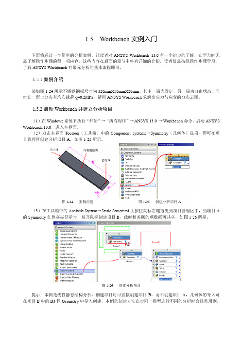
1.5 W orkbench实例入门下面将通过一个简单的分析案例,让读者对ANSYS Workbench 13.0有一个初步的了解,在学习时无需了解操作步骤的每一项内容,这些内容在后面的章节中将有详细的介绍,读者仅需按照操作步骤学习,了解ANSYS Workbench有限元分析的基本流程即可。
1.5.1案例介绍某如图1-24所示不锈钢钢板尺寸为320mmX50mmX20mm,其中一端为固定,另一端为自由状态,同时在一面上分布有均布载荷q=0.2MPa,请用ANSYS Workbench求解出应力与应变的分布云图。
1.5.2启动Workbench并建立分析项目(1)在Windows系统下执行“开始”→“所有程序”→ANSYS 13.0 →Workbench命令,启动ANSYS Workbench 13.0,进入主界面。
(2)双击主界面Toolbox(工具箱)中的Component systems→Symmetry(几何体)选项,即可在项目管理区创建分析项目A,如图1-25所示。
图1-24 案例问题图1-25 创建分析项目A(3)在工具箱中的Analysis System→Static Structural上按住鼠标左键拖曳到项目管理区中,当项目A 的Symmetry红色高亮显示时,放开鼠标创建项目B,此时相关联的项数据可共享,如图1-26所示。
图1-26 创建分析项目提示:本例是线性静态结构分析,创建项目时可直接创建项目B,而不创建项目A,几何体的导入可在项目B中的B3栏Geometry中导入创建。
本例的创建方法在对同一模型进行不同的分析时会经常用到。
1.5.3导入创建几何体(1)在A2栏的Geometry上点击鼠标右键,在弹出的快捷菜单中选择Import Geometry→Browse命令,如图1-27所示,此时会弹出“打开”对话框。
(2)在弹出的“打开”对话框中选择文件路径,导入char01-01几何体文件,如图1-28所示,此时A2栏Geometry后的变为,表示实体模型已经存在。
Workbench实例入门

1.5Workbench实例入门下面将通过一个简单的分析案例,让读者对ANSYS Workbench13.0有一个初步的了解,在学习时无需了解操作步骤的每一项内容,这些内容在后面的章节中将有详细的介绍,读者仅需按照操作步骤学习,了解ANSYS Workbench有限元分析的基本流程即可。
1.5.1案例介绍某如图1-24所示不锈钢钢板尺寸为320mmX50mmX20mm,其中一端为固定,另一端为自由状态,同时在一面上分布有均布载荷q=0.2MPa,请用ANSYS Workbench求解出应力与应变的分布云图。
1.5.2启动Workbench并建立分析项目(1)在Windows系统下执行“开始”→“所有程序”→ANSYS13.0→Workbench命令,启动ANSYS Workbench13.0,进入主界面。
(2)双击主界面Toolbox(工具箱)中的Component systems→Symmetry(几何体)选项,即可在项目管理区创建分析项目A,如图1-25所示。
图1-24案例问题图1-25创建分析项目A(3)在工具箱中的Analysis System→Static Structural上按住鼠标左键拖曳到项目管理区中,当项目A 的Symmetry红色高亮显示时,放开鼠标创建项目B,此时相关联的项数据可共享,如图1-26所示。
图1-26创建分析项目提示:本例是线性静态结构分析,创建项目时可直接创建项目B,而不创建项目A,几何体的导入可在项目B中的B3栏Geometry中导入创建。
本例的创建方法在对同一模型进行不同的分析时会经常用到。
1.5.3导入创建几何体(1)在A2栏的Geometry上点击鼠标右键,在弹出的快捷菜单中选择Import Geometry→Browse命令,如图1-27所示,此时会弹出“打开”对话框。
(2)在弹出的“打开”对话框中选择文件路径,导入char01-01几何体文件,如图1-28所示,此时A2栏Geometry后的变为,表示实体模型已经存在。
ANSYS Workbench入门培训解读
步骤3.填写材料属性 Density密度 Young’s Modulus弹性模量 Poisson’s Ratio泊松比
步骤4.Return Project回到 工程项目管理窗口
双击B4,Model 进入Static Structural— Mechanical
在模型树中选中零件111
分配材料Assignment 选择Gray Cast Iron
进入尺寸标注Dimensions 步骤1.点击 General标注线段长度H1、V2 Horizontal标注水平间距H3 Vertical标注竖直间距V5
步骤2.标注尺寸
步骤3.点击Extrude拉伸
步骤1.Imprint Faces
步骤2.Generate 生成区域面,次面无高度、 无厚度,不影响结构
与Pro/E另一种连接方法
当前面连接方法失败或未连接,可在ANSYS安装好后再连接
2.启动Workbench(两种方式) 1)直接点击开始菜单-程序; 2)进入Pro/E菜单栏启动(较常用)。
Pro/E中先打开零件或组件(必须保证零件无螺纹线、无修饰线,否则无法在 Workbench中打开),再启动Workbench即可导入模型。
屈服极限σs 355 785
从上述数据来看,合金钢只是比碳钢更不易被破坏,即合金钢的安全系 数更高。但在同等拉力作用下,两种的变形量是差不多的,因为它们 的弹性模量差不多。
材料应力应变图
强度理论
1.最大拉应力理论(第一强度理论)(关于断裂的强度理论) 最大拉应力是引起脆性材料断裂的主因,即不论材料处于什么应力状 态下,只要最大拉应力σ1(Maximum Principal 最大应力)达到某个极 限值(强度极限σb)时,材料就会发生脆性断裂。
- 1、下载文档前请自行甄别文档内容的完整性,平台不提供额外的编辑、内容补充、找答案等附加服务。
- 2、"仅部分预览"的文档,不可在线预览部分如存在完整性等问题,可反馈申请退款(可完整预览的文档不适用该条件!)。
- 3、如文档侵犯您的权益,请联系客服反馈,我们会尽快为您处理(人工客服工作时间:9:00-18:30)。
1.5.7 施加载荷 与约束
A
1.5.8 结果后处 理
B
1.5.9 保存与退 出
C
1 初识ANSYS Workbench 13.0
1.5 Workbench实例入门
02
2 创建Workbench几何模型
2 创建Workbench几何模型
2.1 认识 DesignModeler
03
3 Workbench划分网格
3 Workbench划分网格
3.1 网 格划分 平台
3.2 3D 几何网格 划分
3.3 网 格参数 设置
3.4 扫 掠网格 划分
3.5 多 区网格 划分
3.6 网 格划分 案例
3 Workbench 划分网格
3.7 本章小结
3.1.1 网格划分特点 3.1.3 网格划分技巧 3.1.5 网格尺寸策略
2.5.6 偏移横 截面
2 创建Workbench几何模型
2.5.7 从线创建面 体
A
2.5.8 从草图生成 面体
B
2.5.9 从面生成面 体
C
2.5 概念建模
2.6.1 进 入DM界 面
2.6.2 绘 制零件底 部圆盘
2.6.4 生成线 体
2.6.5 生成面 体
2 创建Workbench几何模型
2.6 创建几何体的实例操作
2.6.3 创建零 件肋柱
2.6.6 保 存文件并 退出
2.7.1 从 CAD进入 DM界面
2.7.2 创建线 体
2.7.4 创建横 截面
2.7.5 为 线体添加 横截面
2 创建Workbench几何模型
2.7 概念建模实例操作
2.7.3 生成面 体
2.7.6 保 存文件并 退出
https:///
3.5.1 多区划分 方法
A
3.5.2 多区网格 控制
B
3 Workbe nch划分 网格
3.6 网格划分案例
https:///
3.6.1 自动网格 划分案例
A
3.6.2 网格划分 控制案例
B
04
4 Mechanical基础
2.1.5 DM几何体
2.1.2 DesignModeler的 操作界面
2.1.4 图形选取与控制
2 创建Workbench几何模型
2.1 认识DesignModeler
2 创建Workbench几何模型
2.2.1 创建 新平面
2.2.3 草图 模式
2.2.2 创建 新草图
2.2.4 草图 援引
2.2 DesignModeler草图模 式
2.4 导入外部CAD文件
2.4.1 非关联 性导入文件
2.4.3 导入定 位
2.4.2 关联性 导入文件
2.4.4 创建场 域几何体
2.5.1 从点生 成线体
2.5.2 从 草图生成 线体
2.5.4 定义横 截面
2.5.5 对齐横 截面
2 创建Workbench几何模型
2.5 概念建模
2.5.3 从边生 成线体
ANSYS WorkBench 13.0
从 入 门 到 精 通
演讲人 2 0 2 1 - 11 - 11
01
1 初识ANSYS Workbench 13.0
1 初识ANSYS Workbench 13.0
1
1.1 ANSYS Workbench 13.0概述
2
1.2 Workbench 13.0的基 本操作界面
1.1.4 Workbenc h应用模块
1.1.5 Workbenc h应用方式
1.1 ANSYS Workbench 13.0概述
1 初识ANSYS Workbench 13.0
1.2 Workbench 13.0的基 本操作界面
1
1.2.1 启动ANSYS
Workbench
2
1.2.2 ANSYS
3
1.3 Workbench项目管理
4
1.4 Workbench文件管理
5
1.5 Workbench实例入门
6
1.6 本章小结
1 初识ANSYS Workbench 13.0
0
0
1
2
1.1.1 关于
1.1.2 多
ANSYS
物理场分
Workbench
析模式
0
0
0
3பைடு நூலகம்
4
5
1.1.3 项 目级仿真 参数管理
3.3.3 膨胀控制
3.3.2 尺寸控制 3.3.4 网格信息
3 Workbench划分网格
3.3 网格参数设置
3 Workbe nch划分 网格
3.4 扫掠网格划分
https:///
3.4.1 扫掠划分 方法
A
3.4.2 扫掠网格 控制
B
3 Workbe nch划分 网格
3.5 多区网格划分
3.1.2 网格划分方法 3.1.4 网格划分流程
3 Workbench划分网格
3.1 网格划分平台
3 Workbench划分网格
3.2 3D几何网格划分
A
C
3.2.2 四面体网格 划分时的常用参数
3.2.1 四面体 网格的优缺点
3.2.3 四面体 算法
B
3.2.4 四面体 膨胀
D
3.3.1 缺省参数 设置
https:///
1
1.4.1 文件目录结构
2
1.4.2 快速生成压缩文件
1.5.1 案例介绍
1.5.3 导入创建几何体
1.5.5 添加模型材料属性
1.5.2 启动Workbench并建 立分析项目
1.5.4 添加材料库
1.5.6 划分网格
1 初识ANSYS Workbench 13.0
Workbench主界面
1 初识ANSYS Workbench 13.0
1.3 Workbench项目管理
1.3.1 复制及 删除项目
1.3.3 项目管 理操作案例
1.3.2 关联项 目
1.3.4 设置项 属性
1 初识 ANSYS Workbe nch 13.0
1.4 Workbench文件管 理
2.2 DesignModeler 草图模式
2.3 创建3D几何 体
2.4 导入外部 CAD文件
2.5 概念建模
2.6 创建几何体 的实例操作
2 创建Workbench几何模型
2.7 概念 建模实例操 作
2.8 本章 小结
2.1.1 进入 DesignModeler
2.1.3 DesignModeler的 鼠标操作
2.3.1 创建3D 特征
2.3.2 激 活体和冻 结体
2.3.4 抑制体
2.3.5 面印记
2 创建Workbench几何模型
2.3 创建3D几何体
2.3.3 切片特 征
2.3.6 填 充与包围 操作
2 创建Workbench 几何模型
2.3 创建3D几何体
2.3.7 创建多体部件体
2 创建Workbench 几何模型