矩阵微积分MatrixCalculus

合集下载

Matrix Calculus

AMatrix CalculusA.1Singular value decompositionThe singular value decomposition(SVD)of an M-by-N matrix A is written asA=VΣU T,(A.1) where•V is an orthonormal(or unitary)M-by-M matrix such that V T V=I M×M.•Σis a pseudodiagonal matrix with the same size as A;the M entriesσm on the diagonal are called the singular values of A.•U is an orthonormal(or unitary)N-by-N matrix such that U T U=I N×N. The number of singular values diﬀerent from zero gives the rank of A.When the rank is equal to P,the SVD can be used to compute the(pseudo-)inverse of A:A+=UΣ+V T,(A.2) where the(pseudo-)inverse ofΣis trivially computed by transposing it and inverting its diagonal entriesσm.The SVD is used in many other contexts and applications.For example,principal component analysis(see Section2.4) can be carried out using an SVD.By the way,it is noteworthy that PCA uses a slightly modiﬁed SVD. Assuming that M<N,U could become large when M N,which often happens in PCA,andΣcontains many useless zeros.This motivates an al-ternative deﬁnition of the SVD,called the economy-size SVD,where only the ﬁrst P columns of U are computed.Consequently,U T has the same size as A andΣbecomes a square diagonal matrix.A similar deﬁnition is available when M>N.For a square and symmetric matrix,the SVD is equivalent to the eigenvalue decomposition(EVD;see ahead).248A Matrix CalculusA.2Eigenvalue decompositionThe eigenvalue decomposition(EVD)of a square M-by-M matrix A is written asA V=VΛ,(A.3) where•V is a square M-by-M matrix whose columns v m are unit norm vectors called eigenvectors of A.•Λis a diagonal M-by-M matrix containing the M eigenvaluesλm of A. The EVD is sometimes called the spectral decomposition of A.Equation(A.3) translates the fact the eigenvectors keep their direction after left-multiplication by A:Av m=λm v m.Moreover,the scaling factor is equal to the associated eigenvalue.The number of eigenvalues diﬀerent from zero gives the rank of A,and the product of the eigenvalues is equal to the determinant of A.On the other hand,the trace of A,denoted tr(A)and deﬁned as the sum of its diagonal entries,is equal to the sum of its eigenvalues:tr(A)Mm=1a m,m=Mm=1λm.(A.4)In the general case,even if A contains only real entries,V andΛcan be complex.If A is symmetric(A=A T),then V is orthonormal(the eigen-vectors are orthogonal in addition to being normed);the EVD can then be rewritten asA=VΛV T,(A.5) and the eigenvalues are all real numbers.Moreover,if A is positive deﬁnite (resp.,negative deﬁnite),then all eigenvalues are positive(resp.,negative). If A is positive semideﬁnite(resp.,negative semideﬁnite),then all eigenval-ues are nonnegative(resp.,nonpositive).For instance,a covariance matrix is positive semideﬁnite.A.3Square root of a square matrixThe square root of a diagonal matrix is easily computed by applying the square root solely on the diagonal entries.By comparison,the square root of a nondiagonal square matrix may seem more diﬃcult to compute.First of all, there are two diﬀerent ways to deﬁne the square root of a square matrix A.Theﬁrst deﬁnition assumes thatA (A1/2)T(A1/2).(A.6) If A is symmetric,then the eigenvalue decomposition(EVD)of the matrix helps to return to the diagonal case.The eigenvalue decomposition(see Ap-pendix A.2)of any symmetric matrix A isA.3Square root of a square matrix249A=VΛV T=(VΛ1/2)(Λ1/2V T)=(A1/2)T(A1/2),(A.7)whereΛis diagonal.If A is also positive deﬁnite,then all eigenvalues are positive and the diagonal entries ofΛ1/2remain positive real numbers.(If A is only positive semideﬁnite,then the square root is no longer unique.) The second and more general deﬁnition of the square root is written asA (A1/2)(A1/2).(A.8)Again,the eigenvalue decomposition leads to the solution.The square root is then written asA1/2=VΛ1/2V−1,(A.9) and it is easy to check thatA1/2A1/2=VΛ1/2V−1VΛ1/2V−1(A.10)=VΛ1/2Λ1/2V−1(A.11)=VΛV−1=A.(A.12)This is valid in the general case,i.e.,A can be complex and/or nonsym-metric,yielding complex eigenvalues and eigenvectors.If A is symmetric,the last equation can be further simpliﬁed since the eigenvectors are real and orthonormal(V−1=V T).It is notenorthy that the second deﬁnition of the matrix square root can be generalized to compute matrix powers:A p=VΛp V−1.(A.13)BGaussian VariablesThis appendix brieﬂy introduces Gaussian random variables and some of their basic properties.B.1One-dimensional Gaussian distributionConsidering a single one-dimensional random variable x,it is said to be Gaus-sian if its probability density function f x(x)can be written asf x(x)=1√2πσ2exp−12(x−μ)2σ2,(B.1)whereμandσ2are the mean and the variance,respectively,andcorrespond totheﬁrst-order moment and second-order central moment.Figure B.1shows a plot of a Gaussian probability density function.Visually,the meanμindicates Fig.B.1.Probability density function associated with a one-dimensional Gaussian distribution.252B Gaussian Variablesthe abscissa where the bump reaches its highest point,whereasσis related to the spreading of the bump.For this reason,the standard deviationσis often called the width in a geometrical context(see ahead).Since only the mean and variance suﬃce to characterize a Gaussian vari-able,it is often denoted as N(μ,σ).The letter N recalls the alternative name of a Gaussian variable:a normal variable or normally distributed variable. This name simply reﬂects the fact that for real-valued variables,the Gaussian distribution is the most widely observed one in a great variety of phenomena.Moreover,the central limit theorem states that a variable obtained as the sum of several independent identically distributed variables,regardless of their distribution,tends to be Gaussian if the number of terms in the sum tends to inﬁnity.Thus,to some extent,the Gaussian distribution can be considered the“child”of all other distributions.On the other hand,the Gaussian distribution can also be interpreted as the“mother”of all other distributions.This is intuitively conﬁrmed by the fact that any zero-mean unit variance pdf f y(y)can be modeled starting from a zero-mean and unit-variance Gaussian variable with pdf f x(x),by means of the Gram–Charlier or Edgeworth development:f y(y)=f x(y)1+16μ3(y)H3(y)+124(μ4(y)−3)H4(y)+...,(B.2)where H i(y)is the i th-order Hermitte–Chebyshev polynomial andμi(y)the i th-order central moment.If the last equation is rewritten using the i th-order cumulantsκi(y)instead of central moments,one getsf y(y)=f x(y)1+16κ3(y)H3(y)+124κ4(y)H4(y)+....(B.3)Visually,in the last development,a nonzero skewnessκ3(y)makes the pdf f y(y)asymmetric,whereas a nonzero kurtosis excessκ4(y)makes its bump ﬂatter or sharper.Even if the development does not go beyond the fourth order,it is easy to guess that the Gaussian distribution is the only one having zero cumulants for orders higher than two.This partly explains why Gaussian variables are said to be the“least interesting”ones in some contexts[95]. Actually,a Gaussian distribution has absolutely no salient characteristic:•The support is unbounded,in contrast to a uniform distribution,for in-stance.•The pdf is smooth,symmetric,and unimodal,without a sharp peak like the pdf of a Laplacian distribution.•The distribution maximizes the diﬀerential entropy.The function deﬁned in Eq.(B.1)and plotted in Fig.B.1is the sole func-tion that both shows the above properties and respects the necessary con-ditions to be a probability density function.These conditions are set on the cumulative density function F x(x)of the random variable,deﬁned asB.2Multidimensional Gaussian distribution 253F x (x )=x −∞f x (u )du ,(B.4)and requires that•F x (−∞)=0,•F x (+∞)=1,•F x (x )is monotonic and nondecreasing,•F x (b )−F x (a )is the probability that a <x ≤b .B.2Multidimensional Gaussian distributionA P -dimensional random variable x is jointly Gaussian if its joint probability density function can be written asf x (x )=1 (2π)P det C xxexp −12(x −μx )T C −1xx (x −μx ) ,(B.5)where μx and C xx are,respectively,the mean vector and the covariance ma-trix.As the covariance matrix is symmetric and positive semideﬁnite,its deter-minant is nonnegative.The joint pdf of a two-dimensional Gaussian is drawn in Fig.B.2.Fig.B.2.Probability density function associated with a two-dimensional Gaussian distribution.It can be seen that in the argument of the exponential function,the factor (x −μx )T C −1xx (x −μx )is related to the square of the Mahalanobis distance between x and μx (see Subsection 4.2.1).254B Gaussian VariablesB.2.1Uncorrelated Gaussian variablesIf a multidimensional Gaussian distribution is uncorrelated,i.e.,if its covari-ance matrix is diagonal,then the last equation can be rewritten asf x(x)=1(2π)PPp=1c p,pexp−12Pp=1(x p−μx p)2c2p,p(B.6)=Pp=112πc p,pexp−12(x p−μx p)2c p,p(B.7)=Pp=112πσxpexp−12(x p−μx p)2σ2xp(B.8)=Pp=1f xp(x p),(B.9)showing that the joint pdf of uncorrelated Gaussian variables factors into the product of the marginal probability density functions.In other words,uncor-related Gaussian variables are also statistically independent.Again,f x(x)is the sole and unique probability density function that can satisfy this property. For other multivariate distributions,the fact of being uncorrelated does not imply the independence of the marginal densities.Nevertheless,the reverse implication is always true.Geometrically,a multidimensional Gaussian distribution looks like a fuzzy ellipsoid,as shown in Fig.B.3.The axes of the ellipsoid correspond to coor-dinate axes.B.2.2Isotropic multivariate Gaussian distributionA multidimensional Gaussian distribution is said to be isotropic if its covari-ance matrix can be written as a function of the single parameterσ:C xx=σ2I.(B.10) As C xx is diagonal,the random variables in x are uncorrelated and inde-pendent,andσis the common standard deviation shared by all marginalprobability density functions f xp (x p).By comparison to the general case,thepdf of an isotropic Gaussian distribution can be rewritten more simply asf x(x)=1(2π)P det(σ2I)exp−12(x−μx)T(σ2I)−1(x−μx)(B.11)=1(2πσ2)Pexp−12(x−μx)T(x−μx)σ2(B.12)=1(2πσ2)Pexp−12x−μx 22σ2,(B.13)B.2Multidimensional Gaussian distribution 255Fig.B.3.Sample joint distribution (10,000realizations,in blue)of two uncorrelated Gaussian variables.The variances are proportional to the axis lengths (in red).The appearance of the Euclidean distance (seeSubsection 4.2.1)demonstrates that the value of the pdf depends only on the distance to the mean and not on the orientation.Consequently,f x (x )is completely isotropic:no direction is privileged,as illustrated in Fig.B.4.For this reason,the standard deviationFig. B.4.Sample (10,000realizations)of a two-dimensional isotropic Gaussian distribution.The variances are proportional to the axis lengths (in red),which are equal.The variance is actually the same in all directions.σis often called the width or radius of the Gaussian distribution.256B Gaussian VariablesThe function f x(x)is often used outside the statistical framework,possibly without its normalization factor.In this case,f x(x)is usually called a radial basis function or Gaussian kernel.In addition to be isotropic,such a function has very nice properties:•It produces a single localized bump.•Very few parameters have to be set(P means and one single variance, compared to P(P+1)/2for a complete covariance matrix).•It depends on the well-known and widely used Euclidean distance. Gaussian kernels are omnipresent in applications like radial basis function networks[93](RBFNs)and support vector machines(SVM)[27,37,42]. B.2.3Linearly mixed Gaussian variablesWhat happens when several Gausian variables are linearly mixed?To answer the question,one assumes that the P-dimensional random vec-tor x has a joint Gaussian distribution with zero means and identity covari-ance,without loss of generality.Then P linearly mixed variables can be written as y=Ax,where A is a square P-by-P mixing matrix.By“mixing matrix”, it should be understood that A is of full column rank and has at least two nonzero entries per row.These conditions ensure that the initial random vari-ables are well mixed and not simply copied or scaled.It is noteworthy that y has zero means like x.As matrix A deﬁnes a nonorthogonal change of the axes,the joint pdf of y can be written asf y(y)=1(2π)P det C yyexp−12y T I−1y(B.14)=1(2π)P det C yyexp−12(Ax)T(Ax)(B.15)=1(2π)P det C yyexp−12x T(A T A)x),(B.16)demonstrating that C yy=(A T A)−1.Unfortunately,as the covariance matrix is symmetric,it has only P(P+1)/2free parameters,which is less than P2, the number of entries in the mixing matrix A.Consequently,starting from the mixed variables,it is impossible to retrieve the mixing matrix.A possible solution would have been to compute the matrix square root of C−1yy(see Subsection A.3).However,this provides only a least-squares estimate of A, on the basis of the incomplete information available in the covariance matrix. Geometrically,one sees in Fig.B.5that the matrix square root alwaysﬁnds an orthogonal coordinate system,computed as the eigenvetors of C−1yy.This orthogonal system is shown in red,whereas the original coordinate system deformed by the mixing matrix is drawn in green.This explains why PCAB.2Multidimensional Gaussian distribution257Fig.B.5.Sample joint distribution(10,000realizations)of two isotropic Gaussian variables.The original coordinate system,in green,has been deformed by the mixing matrix.Any attempt to retrieve it leads to the orthogonal system shown in red. (and ICA)is unable to separate mixtures of Gaussian variables:with two or more Gaussian variables,indeterminacies appear.COptimizationMost nonspectral NLDR methods rely on the optimization of some objective function.This appendix describes a few classical optimization techniques. C.1Newton’s methodThe original Newton’s method,also known as Newton–Raphson method,is an iterative procedure thatﬁnds a zero of a C∞function(inﬁnitely diﬀerentiable function)f:R→R:x→f(x).(C.1) Basically,Newton’s method approximates the function f by itsﬁrst-order Taylor’s polynomial expansion:f(x+ )=f(x)+f (x) +O( 2).(C.2)Deﬁning xold =x and xnew=x+ ,omitting O( 2),and assuming thatf(xnew)=0,one gets:0≈f(xold )+f (xold)(xnew−x old).(C.3)Solving for xnewleads tox new≈x old−f(x old)f (xold,(C.4)which can be rewritten as an iterative update rule:x←x−f(x)f (x).(C.5)Intuitively,starting from a candidate solution x that is randomly initialized, the next candidate is the intersection of a tangent to f(x)with the x-axis. It can be proven that theﬁrst-order approximation makes the convergence of the procedure very fast(quadratic convergence):after a few iterations, the solution remains almost constant,and the procedure may be stopped. However,it is easy to see that the method becomes unstable when f (x)≈0.260C OptimizationC.1.1Finding extremaRecalling that function extremas are such that f (x)=0,a straight extension of Newton’s procedure can be applied toﬁnd a local extremum of a twicelyderivable function f:x←x−f (x)f (x),(C.6)where theﬁrst and second derivatives are assumed to be continuous.The last update rule,unfortunately,does not distinguish between a minimum and a maximum and yields either one of them.An extremum is a minimum only if the second derivative is positive,i.e.,the function is concave in the neighbor-hood of the extremum.In order to avoid the convergence toward a maximum, a simple trick consists of forcing the second derivative to be positive:x←x−f (x)|f (x)|.(C.7)C.1.2Multivariate versionThe generalization of Newton’s optimization procedure(Eq.(C.6))to multi-variate functions f(x):R P→R:x→f(x)leads tox←x−H−1∇x f(x),(C.8) where∇x is the diﬀerential operator with respect to the components of vectorx=[x1,...,x P]T:∇x∂∂x1,...,∂∂x PT,(C.9)and∇x f(x)is the gradient of f,i.e.,the vector of all partial derivatives:∇x f(x)=∂f(x)∂x =∂f(x)∂x1,...,∂f(x)∂x PT.(C.10)One step further,H−1is the inverse of the Hessian matrix,deﬁned asH ∇x∇T x f(x)=∂2f(x)∂x i∂x jij,(C.11)whose entries h i,j are the second-order partial derivatives.Unfortunately,the application of Eq.(C.8)raises two practical diﬃculties. First,the trick of the absolute value is not easily generalized to multivariate functions,which can have minima,maxima,but also various kinds of saddle points.Second,the Hessian matrix is rarely available in practice.Moreover, its size grows proportionally to P2,making its computation and storage prob-lematic.C.2Gradient ascent/descent261A solution to these two issues consists of assuming that the Hessian matrix is diagonal,although it is often a very crude hypothesis.This approximation, usually called quasi-Newton or diagonal Newton,can be written component-wise:x p←x p−α∂f(x)∂x p∂2f(x)∂x2p,(C.12)where the coeﬃcientα(0<α≤1)slows down the update rule in order to avoid unstable behaviors due to the crude approximation of the Hessian matrix.C.2Gradient ascent/descentThe gradient descent(resp.,ascent)is a generic minimization(resp.,maxi-mization)technique also known as the steepest descent(ascent)method.As Newton’s method(see the previous section),the gradient descent is an itera-tive technique thatﬁnds the closest extremum starting from an initial guess. The method requires knowing only the gradient of the function to be opti-mized in closed form.Actually,the gradient descent can be seen as a simpliﬁed version of New-ton’s method,in the case where the Hessian matrix is unknown.Hence,the gradient descent is a still rougher approximation than the pseudo-Newton method.More formally,the inverse H−1of the unknown Hessian is simply replaced with the productαI,whereαis a parameter usually called the step size or the learning rate.Thus,for a multivariate function f(x),the iterative update rule can be written asx←x−α∇x f(x).(C.13) As the Hessian is unknown,the local curvature of the function is unknown, and the choice of the step size may be critical.A value that is too large may jeopardize the convergence on an extremum,but,on the other hand,the convergence becomes very slow for small values.C.2.1Stochastic gradient descentWithin the framework of data analysis,it often happens that the function to be optimized is of the formf(x)=E y{g(y,x)}or f(x)=1NNi=1g(y(i),x),(C.14)where y is an observed variable and Y=[...,y(i),...]1≤i≤N is an array of observations.Then the update rule for the gradient descent with respect to the unknown variables/parameters x can be written as262C Optimizationx←x−α∇x 1NNi=1g(y(i),x)}.(C.15)This is the usual update rule for the classical gradient descent.In the frame-work of neural networks and other adaptive methods,the classical gradient descent is often replaced with the stochastic gradient descent.In the latter method,the update rule can be written in the same way as in the classical method,except that the mean(or expectation)operator disappears:x←x−α∇x g(y(i),x).(C.16) Because of the dangling index i,the update rule must be repeated N times, over all available observations y(i).From an algorithmic point of view,this means that two loops are needed.Theﬁrst one corresponds to the iterations that are already performed in the classical gradient descent,whereas an inner loop traverses all vectors of the data set.A traversal of the data set is usually called an epoch.Moreover,from a theoretical point of view,as the partial updates are no longer weighted and averaged,additional conditions must be fulﬁlled in order to attain convergence.Actually,the learning rateαmust decrease as epochs go by and,assuming t is an index over the epochs,the following(in)equalities must hold[156]:∞t=1α(t)=∞and∞t=1(α(t))2<∞.(C.17)Additionally,it is often advised to consider the available observations as an unordered set,i.e.,to randomize the order of the updates at each epoch.This allows us to avoid any undesired bias due to a repeated order of the updates.When a stochastic gradient descent is used in a truly adaptive context, i.e.,the sequence of observations y(i)is inﬁnite,then the procedure cannot be divided into successive epochs:there is only a single,very long epoch.In that case the learning rate is set to a small constant value(maybe after a short decrease starting from a larger value in order to initialize the process). Conditions to attain convergence are diﬃcult to study in that case,but they are generally fulﬁlled if the sequence of observations is stationary.DVector quantizationLike dimensionality reduction,vector quantization[77,73]is a way to re-duce the size of a data set.However,instead of lowering the dimensionality of the observations,vector quantization reduces the number of observations (see Fig.D.1).Therefore,vector quantization and dimensionality reduction are somewhat complementary techniques.By the way,it is noteworthy that several DR methods use vector quantization as preprocessing.In practice,vector quantization is achieved by replacing the original data points with a smaller set of points called units,centroids,prototypes or code vectors.The ordered or indexed set of code vectors is sometimes called the codebook.Intuitively,a good quantization must show several qualities.Classically, the user expects that the prototypes are representative of the original data they replace(see Fig.D.1).More formally,this goal is reached if the prob-ability density function of the prototypes resembles the probability density function of the initial data.However,as probability density functions are dif-ﬁcult to estimate,especially when working with aﬁnite set of data points, this idea will not work as such.An alternative way to capture approximately the original density consists of minimizing the quantization distortion.For a data set Y={y(i)∈R D}1≤i≤N and a codebook C={c(j)∈R D}1≤j≤M,the distortion is a quadratic error function written asEVQ =1NNi=1y(i)−dec(cod(y(i))) 2,(D.1)where the coding and decoding functions cod and dec are respectively deﬁned ascod:R D→{1,...,M}:y→arg min1≤j≤My−c(j) (D.2) anddec:{1,...,M}→C:j→c(j).(D.3)264D Vector quantizationFig.D.1.Principle of vector quantization.Theﬁrst plot shows a data set(2000 points).As illustrated by the second plot,a vector quantization method can reduce the number of points by replacing the initial data set with a smaller set of repre-sentative points:the prototypes,centroids,or code vectors,which are stored in the codebook.The third plot shows simultaneously the initial data,the prototypes,and the boundaries of the corresponding Vorono¨ıregions.D.1Classical techniques265 The application of the coding function to some vector y(i)of the data set gives the index j of the best-matching unit of y(i)(BMU in short),i.e.,the closest prototype from y(i).Appendix F.2explains how to compute the BMU eﬃciently.The application of the decoding function to j simply gives the coordinates c(j)of the corresponding prototype.The coding function induces a partition of R D:the open sets of all points in R D that share the same BMU c(j)are called the Vorono¨ıregions(see Fig.D.1).A discrete approximation of the Vorono¨ıregions can be obtained by constituting the sets V j of all data points y(i)having the same BMU c(j).Formally,these sets are written asV j={y(i)|cod(y(i))=j}(D.4) and yield a partition of the data set.D.1Classical techniquesNumerous techniques exist to minimize EVQ.The most prominent one is the LBG algorithm[124],which is basically an extension of the generalized Lloyd method[127].Close relatives coming from the domain of cluster analysis are the ISODATA[8]and the K-means[61,130]algorithms.In the case of the K-means,the codebook is built as follows.After the initialization(see ahead), the following two steps are repeated until the distortion decreases below a thresholdﬁxed by the user:1.Encode each point of the data set,and compute the discrete Vorono¨ıregions V j;2.Update each c(j)by moving it to the barycenter of V j,i.e.,c(j)←1|V j|y(i)∈V jy(i).(D.5)This procedure monotonically decreases the quantization distortion until it reaches a local minimum.To prove the correctness of the procedure,one rewrites EVQas a sum of contributions coming from each discrete Vorono¨ıregion:EVQ =1NMj=1E jVQ,(D.6)whereE jVQ =y(i)∈V jy(i)−c(j) 2.(D.7)Trivially,the barycenter of some V j minimizes the corresponding E jVQ.There-fore,step2decreases EVQ.But,as a side eﬀect,the update of the prototypes also modiﬁes the results of the encoding function.So it must be shown that the266D Vector quantizationre-encoding occurring in step1also decreases the distortion.The only terms that change in the quantization distortion deﬁned in Eq.(D.1)are those cor-responding to data points that change their BMU.By deﬁnition of the coding function,the distance y(i)−c(j) is smaller for the new BMU than for the old one.Therefore,the error is lowered after re-encoding,which concludes the correctness proof of the K-means.D.2Competitive learningFalling in local minima can be avoided to some extent by minimizing the quantization distortion by stochastic gradient descent(Robbins–Monro pro-cedure[156]).For this purpose,the gradient of EVQwith respect to prototype c(j)is written as∇c(j)E VQ=1NNi=12 y(i)−c(j)∂ y(i)−c(j)∂c(j)(D.8)=1NNi=12 y(i)−c(j)(c(j)−y(i))2 y(i)−c(j)(D.9)=1NNi=1(c(j)−y(i)),(D.10)where the equality j=cod(y(i))holds implicitly.In a classical gradient de-scent,all prototypes are updated simultaneously after the computation of their corresponding gradient.Instead,the Robbins–Monro procedure[156](or stochastic gradient descent)separates the terms of the gradient and updates immediately the prototypes according to the simple rule:c(j)←c(j)−α(c(j)−x i),(D.11) whereαis a learning rate that decreases after each epoch,i.e.,each sweeping of the data set.In fact,the decrease of the learning rateαmust fulﬁll the conditions stated in[156](see Section C.2).Unlike the K-means algorithm,the stochastic gradient descent does not decrease the quantization distortion monotonically.Actually,the decrease oc-curs only on average.The stochastic gradient descent of EVQbelongs to a wide class of vector quantization algorithms known as competitive learning methods[162,163,3].D.3TaxonomyQuantization methods may be divided into static,incremental,and dynamic ones.This distinction refers to their capacity to increase or decrease the num-ber of prototypes they update.Most methods,like competitive learning and。

微积分与矩阵

微积分学（Calculus，拉丁语意为用来计数的小石头）是研究极限、微分学、积分学和无穷级数等的一个数学分支，并成为了现代大学教育的重要组成部分。

微积分学基本定理指出，微分和积分互为逆运算，这也是两种理论被统一成微积分学的原因。

我们可以以两者中任意一者为起点来讨论微积分学，但是在教学中一般会先引入微分学。

在更深的数学领域中，高等微积分学通常被称为分析学，并被定义为研究函数的科学，是现代数学的主要分支之一。

早在古代，人们就会积分思想，如阿基米德用积分法算出了球的表面积，中国古代数学家刘微运用割元法求出圆周率3.1416，这也是用正多边形逼近圆，任何求出近似圆周率。

割圆法也是积分思想。

我们最伟大的古代数学家（现在是华罗庚）祖冲之也是利用积分算出了圆周率后7位数。

和球的体积。

但是正正系统提出微积分的是牛顿和莱布尼茨，他们为谁先发明微积分挣得头破血流。

牛顿是三大数学家之一，也是第一位划时代的物理学家，晚年从事神学和炼金学，它创立了整个经典力学体系和几何光学，这几乎成为了整个中学的必修部分，初中的力学和光学默认为几何光学，力学默认为简单的经典力学。

高中开始正式学习经典力学。

这里有一个非常之大的错误就是初中里为了方便或简单，用平均速率来代替平均速度，也就是速度公式v=x/t在初中里用速率公式v=s/t代替。

速度和速率一个是矢量，一个是标量，这里差距巨大，不知道编写初中课本（人教版是这样）的编者是学历太低，还是别有用心?这里我们讲微积分，之所以提起这个事情，就是为了突出一个名词——平均速度。

牛顿发明微积分（暂且认为是他和莱布尼茨共同发明的）的目的是为了研究物理学，因为微积分能解决很多普通数学不能解决的物体，如求曲边梯形面积。

实际上，我们初中是速度公式是速率公式，即v=s/t高中的速度公式实际上是平均速度公式，即v=△x/△t这里的△念德耳塔，表示变化率，这里当然不是用△去乘x了，△x是一个整体，就像汉字一样。

机器学习算法原理——矩阵微积分，构建你的“黑客帝国”

机器学习算法原理——矩阵微积分，构建你的“黑客帝国”你吃了蓝色的药丸，故事就结束了，你在床上醒来，相信你愿意相信的一切。

你吃了红色的药丸…你留在仙境，我让你看看兔子洞有多深。

这是《黑客帝国》中墨菲斯对尼奥说的名言。

你必须做出同样的选择，你想继续使用像pytorch和tensorflow这样的自动化框架而不知道其背后原理？还是想更深入地研究矩阵计算的世界，了解反向传播算法（ backpropagation，BP）的工作原理？线性代数基础知识向量和矩阵这里，我用不加粗的小写字母表示标量，如：列向量会用加粗的小写字母表示，如：行向量也用加粗的小写字母表示，但它们有一个T上标。

T上标代表转置：代表矩阵的符号将是加粗的大写字母：也可以对一个矩阵进行转置，第一列会变成第一行，反之亦然：一个向量或矩阵的维度是一个元组（行数, 列数）。

让我们考虑下面的情况。

点积点积也是为向量和矩阵定义的。

但顺序很重要，左边的向量/矩阵的列数必须与右边的向量/矩阵的行数一致。

结果的维度是（左边输入的行数，右边输入的列数）如果你有兴趣，下面更详细的点积是如何进行的。

为了得到输出的一个元素，我们将左边的一行和右边的一列向量/矩阵相乘并求和。

点积的重要性在于，它可以在许多不同的情况下使用。

在力学中，它可以用来表示一个物体的旋转和拉伸。

它也可以用来改变坐标系。

分析基础知识和的导数当我们想求一个和的导数时，相当于求每个加数的导数。

乘积法则如果我们想求两个函数的乘积的导数，这两个函数都取决于我们想微分的变量，我们可以使用以下规则。

让我们考虑下面的例子：那么y相对于y的导数是：链式法则我们要对一个函数y进行微分。

这个函数取决于y，y取决于y。

然后，我们可以应用链式法则：让我们在这里做一个简单的练习：矩阵微积分了解这么多基础知识后，我希望你已经准备好进行矩阵微积分了！我们可以用两种方式来写矩阵微积分，即所谓的"分子布局（numerator layout）"和 "分母布局（denominator layout）"。

矩阵微积分基础知识

矩阵微积分基础知识矩阵微积分是数学中重要的分支之一，它将矩阵理论与微积分方法相结合，为解决实际问题提供了强大的工具。

本文将介绍矩阵微积分的基础知识，包括矩阵的定义、矩阵的运算、矩阵的微分和积分等内容，帮助读者更好地理解和应用矩阵微积分。

一、矩阵的定义矩阵是一个按照长方阵列排列的数，是数的一个矩形排列。

一般形式为m×n的矩阵，其中m表示矩阵的行数，n表示矩阵的列数。

矩阵通常用大写字母表示，如A、B、C等。

矩阵中的每一个元素都可以用下标表示，如Aij表示矩阵A中第i行第j列的元素。

二、矩阵的运算1. 矩阵的加法：对应位置的元素相加，要求两个矩阵的行数和列数相等。

例如，设矩阵A = [1 2 3; 4 5 6]，矩阵B = [7 8 9; 10 11 12]，则A + B = [8 10 12; 14 16 18]。

2. 矩阵的数乘：矩阵中的每个元素乘以一个数。

例如，设矩阵A = [1 2; 3 4]，数k = 2，则kA = [2 4; 6 8]。

3. 矩阵的乘法：矩阵乘法不满足交换律，要求左边矩阵的列数等于右边矩阵的行数。

例如，设矩阵A = [1 2; 3 4]，矩阵B = [5 6; 7 8]，则AB =[19 22; 43 50]。

三、矩阵的微分矩阵的微分是矩阵微积分中的重要内容，它可以帮助我们求解矩阵函数的导数。

设矩阵函数F(X) = [f1(X), f2(X), ..., fn(X)]，其中X是一个矩阵变量，fi(X)表示矩阵X的第i个元素函数。

则矩阵函数F(X)的微分定义为：dF(X) = [df1(X), df2(X), ..., dfn(X)]其中dfi(X)表示fi(X)对X的微分。

矩阵函数的微分满足线性性质和Leibniz法则。

四、矩阵的积分矩阵的积分是矩阵微积分中的另一个重要内容，它可以帮助我们求解矩阵函数的不定积分和定积分。

设矩阵函数F(X) = [f1(X),f2(X), ..., fn(X)]，则矩阵函数F(X)的不定积分定义为：∫F(X)dX = [∫f1(X)dX, ∫f2(X)dX, ..., ∫fn(X)dX]其中∫fi(X)dX表示fi(X)对X的不定积分。

矩阵微积分

矩阵微积分本文摘译自 Wikipedia。

在数学中，矩阵微积分是多元微积分的一种特殊表达形式。

它以向量或矩阵的形式将单个函数表示为多个变量，或将一个多元函数表示为单个变量，从而可以作为一个整体来处理，大大简化了多元函数极值、微分方程等问题的求解过程。

表示法在本文中，将采用如下所示的表示方法：•$ \mathbf A, \mathbf X, \mathbf Y $ 等：粗体的大写字母，表示一个矩阵；•$ \mathbf a, \mathbf x, \mathbf y $ 等：粗体的小写字母，表示一个向量；•$ a, x, y $ 等：斜体的小写字母，表示一个标量；•$ \mathbf X^T $：表示矩阵 $ \mathbf X $ 的转置；•$ \mathbf X^H $：表示矩阵 $ \mathbf X $ 的共轭转置；•$ | \mathbf X | $：表示方阵 $ \mathbf X $ 的行列式；•$ || \mathbf x || $：表示向量 $ \mathbf x $ 的范数；•$ \mathbf I $：表示单位矩阵。

向量微分向量-标量列向量函数 $ \mathbf y = \begin{bmatrix} y_1 & y_2 & \cdots & y_m \end{bmatrix}^T $ 对标量 $ x $ 的导数称为$ \mathbf y $ 的切向量，可以以分子记法表示为$ \frac{\partial \mathbf y}{\partial x} =\begin{bmatrix}\frac{\partial y_1}{\partial x}\newline \frac{\partial y_2}{\partial x} \newline\vdots \newline \frac{\partial y_m}{\partialx}\end{bmatrix}_{m \times 1} $若以分母记法则可以表示为$ \frac{\partial \mathbf y}{\partial x} =\begin{bmatrix}\frac{\partial y_1}{\partial x} &\frac{\partial y_2}{\partial x} & \cdots &\frac{\partial y_m}{\partial x}\end{bmatrix}_{1 \times m} $标量-向量标量函数 $ y $ 对列向量 $ \mathbf x = \begin{bmatrix} x_1 & x_2 & \cdots & x_n \end{bmatrix}^T $ 的导数可以以分子记法表示为$ \frac{\partial y}{\partial \mathbf x} =\begin{bmatrix}\frac{\partial y}{\partial x_1} &\frac{\partial y}{\partial x_2} & \cdots &\frac{\partial y}{\partial x_n}\end{bmatrix}_{1 \times n} $若以分母记法则可以表示为$ \frac{\partial y}{\partial \mathbf x} =\begin{bmatrix}\frac{\partial y}{\partial x_1}\newline \frac{\partial y}{\partial x_2} \newline\vdots \newline \frac{\partial y}{\partialx_n}\end{bmatrix}_{n \times 1} $向量-向量列向量函数 $ \mathbf y = \begin{bmatrix} y_1 & y_2 & \cdots & y_m \end{bmatrix}^T $ 对列向量 $ \mathbf x = \begin{bmatrix} x_1 & x_2 & \cdots & x_n\end{bmatrix}^T $ 的导数可以以分子记法表示为$ \frac{\partial \mathbf y}{\partial \mathbf x} =\begin{bmatrix}\frac{\partial y_1}{\partial x_1} &\frac{\partial y_1}{\partial x_2} & \cdots &\frac{\partial y_1}{\partial x_n}\newline\frac{\partial y_2}{\partial x_1} &\frac{\partial y_2}{\partial x_2} & \cdots &\frac{\partial y_2}{\partial x_n} \newline\vdots &\vdots & \ddots & \vdots \newline\frac{\partialy_m}{\partial x_1} & \frac{\partial y_m}{\partial x_2} & \cdots & \frac{\partial y_m}{\partial x_n}\newline\end{bmatrix}_{m \times n} $若以分母记法则可以表示为$ \frac{\partial \mathbf y}{\partial \mathbf x} =\begin{bmatrix}\frac{\partial y_1}{\partial x_1} &\frac{\partial y_2}{\partial x_1} & \cdots &\frac{\partial y_m}{\partial x_1}\newline\frac{\partial y_1}{\partial x_1} &\frac{\partial y_2}{\partial x_1} & \cdots &\frac{\partial y_m}{\partial x_1} \newline\vdots &\vdots & \ddots & \vdots \newline\frac{\partialy_1}{\partial x_1} & \frac{\partial y_2}{\partial x_1} & \cdots & \frac{\partial y_m}{\partial x_1}\newline\end{bmatrix}_{n \times m} $矩阵微分矩阵-标量形状为 $ m \times n $ 的矩阵函数 $ \mathbf Y $ 对标量$ x $ 的导数称为 $ \mathbf Y $ 的切矩阵，可以以分子记法表示为$ \frac{\partial \mathbf Y}{\partial x} =\begin{bmatrix}\frac{\partial y_{11}}{\partial x} &\frac{\partial y_{12}}{\partial x} & \cdots &\frac{\partial y_{1n}}{\partial x}\newline\frac{\partial y_{21}}{\partial x} &\frac{\partial y_{22}}{\partial x} & \cdots &\frac{\partial y_{2n}}{\partial x} \newline\vdots &\vdots & \ddots & \vdots \newline\frac{\partialy_{m1}}{\partial x} & \frac{\partial y_{m2}}{\partial x} & \cdots & \frac{\partial y_{mn}}{\partial x}\newline\end{bmatrix}_{m \times n} $标量-矩阵标量函数 $ y $ 对形状为 $ p \times q $ 的矩阵$ \mathbf X $ 的导数可以分子记法表示为$ \frac{\partial y}{\partial \mathbf X} =\begin{bmatrix}\frac{\partial y}{\partial x_{11}} &\frac{\partial y}{\partial x_{21}} & \cdots &\frac{\partial y}{\partial x_{p1}}\newline\frac{\partial y}{\partial x_{12}} &\frac{\partial y}{\partial x_{22}} & \cdots &\frac{\partial y}{\partial x_{p2}} \newline\vdots &\vdots & \ddots & \vdots \newline\frac{\partialy}{\partial x_{1q}} & \frac{\partial y}{\partialx_{2q}} & \cdots & \frac{\partial y}{\partial x_{pq}} \newline\end{bmatrix}_{q \times p} $若以分母记法则可以表示为$ \frac{\partial y}{\partial \mathbf X} =\begin{bmatrix}\frac{\partial y}{\partial x_{11}} &\frac{\partial y}{\partial x_{12}} & \cdots &\frac{\partial y}{\partial x_{1q}}\newline\frac{\partial y}{\partial x_{21}} &\frac{\partial y}{\partial x_{22}} & \cdots &\frac{\partial y}{\partial x_{2q}} \newline\vdots &\vdots & \ddots & \vdots \newline\frac{\partialy}{\partial x_{p1}} & \frac{\partial y}{\partialx_{p2}} & \cdots & \frac{\partial y}{\partial x_{pq}} \newline\end{bmatrix}_{p \times q} $恒等式在下面的公式中，除非另有说明，默认要导出的复合函数的所有因子都不是导数变量的函数。

Matrix Calculate

ym
where each component yi may be a function of all the x j , a fact represented by saying that y is a function of x, or y = y(x). (F.2) If n = 1, x reduces to a scalar, which we call x . If m = 1, y reduces to a scalar, which we call y . Various applications are studied in the following subsections. §F.2.1. Derivative of Vector with Respect to Vector The derivative of the vector y with respect to vector x is the n × m matrix ∂ y1 ∂ y2 ∂y · · · ∂ xm ∂ x ∂ x 1 1 1 ∂ y1 ∂ y2 ∂ ym ∂ y def ∂ x2 ∂ x2 · · · ∂ x2 = . ∂x . . .. . . . . . . . ∂ ym ∂ y1 ∂ y2 ∂ xn ∂ xn · · · ∂ xn §F.2.2. Derivative of a Scalar with Respect to Vector If y is a scalar, ∂y ∂ x1 ∂y ∂ y def ∂x = 2 ∂x . . . ∂y ∂ xn .
(F.17)
∂2 y = ∂ x2
(F.18)
The following table collects several useful vector derivative formulas. y Ax xT A xT x xT Ax ∂y ∂x AT A 2x Ax + AT x

微积分与矩阵

微积分学基本定理指出，微分和积分互为逆运算，这也是两种理论被统一成微积分学的原因。

我们可以以两者中任意一者为起点来讨论微积分学，但是在教学中一般会先引入微分学。

在更深的数学领域中，高等微积分学通常被称为分析学，并被定义为研究函数的科学，是现代数学的主要分支之一。

割圆法也是积分思想。

我们最伟大的古代数学家（现在是华罗庚）祖冲之也是利用积分算出了圆周率后7位数。

和球的体积。

但是正正系统提出微积分的是牛顿和莱布尼茨，他们为谁先发明微积分挣得头破血流。

高中开始正式学习经典力学。

这里有一个非常之大的错误就是初中里为了方便或简单，用平均速率来代替平均速度，也就是速度公式v=x/t在初中里用速率公式v=s/t代替。

MATRIX CALCULATION

eps 相对精度 i,j 复数中的虚数单位 pi 圆周率π realmax 计算机能够显示的最大浮点数 realmin 计算机能够显示的最小浮点数 version 字符串格式的MATLAB版本
14
错误提示信息说明 singular 奇异阵 Badly scaled 病态阵 inf Matlab用来表示无穷大的专用变量，可以避免零溢出（zero overflow） Inner matrix dimensions must agree 矩阵相乘出错：维数不对
c=a' c=a.'
22
三、关系运算和逻辑运算
MATLAB对此类运算符有如下规定：所有的关系表达式或逻辑表达式中，任何非0 数都是“逻辑真”，只有0才是“逻辑假” 关系表达式或逻辑表达式的计算结果是一个由0和1组成的“逻辑数组(Logical Array)”,数组中1表示真，0表示假逻辑数组是一种特殊的数值数组，对“数值数组”操作有关命令和函数也适用它；同时又具有自身的特殊用途优先级别：算术运算关系运算逻辑运算
21
7、矩阵的转置
a' 或 a. '
a': 矩阵a的共轭转置
a. ': 矩阵a的转置
若a是实数矩阵，则a'==a. '
【例2-14】矩阵a为[1 2 3;4 5 6;7 8 9],计算a的转置
a=[1 2 3;4 5 6;7 8 9]; c=a'
【例2-15】矩阵a为[1+2i 3+4i],计算a的转置。 a=[1+2i 3+4i];
数组B与标量c间的乘除运算
c.*B ==B.*c: B的每一个元素乘以c c./B==B.\c : c除以 B的每一个元素 c.\B ==B./c: B的每一个元素除以c

矩阵的微分与积分

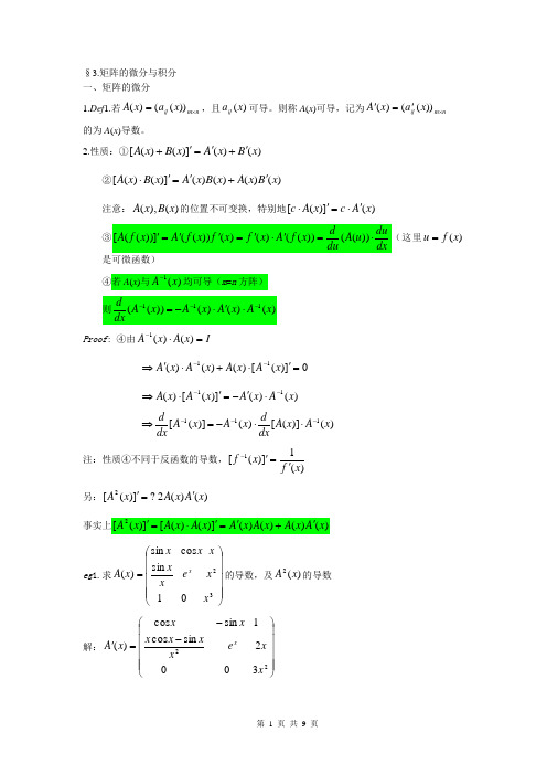
§3.矩阵的微分与积分一、矩阵的微分1.Def 1.若n m ij x a x A ⨯=))(()(，且)(x a ij 可导。

则称A (x )可导，记为n m ijx a x A ⨯'='))(()( 的为A (x )导数。

2.性质：①)()(])()([x B x A x B x A '+'='+②)()()()(])()([x B x A x B x A x B x A '+'='⋅注意：)(),(x B x A 的位置不可变换，特别地)(])([x A c x A c '⋅='⋅)(x f u =是可微函数）④若A (x )与)(1x A -均可导（m =n 方阵）Proof : ④由I x A x A =⋅-)()(10])([)()()(11='⋅+⋅'⇒--x A x A x A x A )()(])([)(11x A x A x A x A --⋅'-='⋅⇒)()]([)()]([111x A x A dxdx A x A dx d ---⋅⋅-=⇒注：性质④不同于反函数的导数，)(1])([1x f x f '='- 另：)()(2?])([2x A x A x A '='事实上)()()()(])()([])([2x A x A x A x A x A x A x A '+'='⋅='eg 1.求⎪⎪⎪⎪⎪⎭⎫ ⎝⎛=3201sin cos sin )(x x e xx x x x x A x 的导数，及)(2x A 的导数解：⎪⎪⎪⎪⎪⎭⎫⎝⎛--='223002sin cos 1sin cos )(x x e x xx x x x x A x)()()()(])([2x A x A x A x A x A '+'='⎪⎪⎪⎪⎪⎪⎪⎭⎫ ⎝⎛+-+++++-+-++-+-+-+-+=52242222232261sin 3cos )2(5cos 22sin 2cos 22sin )cos (sin sin 2sin 4sin )1(cos 32sin 2cos 122sin 2cos 22sin x x x x e x x x x e x x x x x e x x x x x x x x x x x x x x x x x x x x xx xeg2.设⎪⎪⎭⎫⎝⎛-=x xx xx A sin cos cos sin )( 求)]([1x A dx d -，)]([2x A dx d 解：⎪⎪⎭⎫⎝⎛-=-x x x x x A sin cos cos sin )(1 ⎪⎪⎭⎫ ⎝⎛-=-x x x x x A dx d cos sin sin cos )]([1)()(22sin 2cos 2cos 2sin 22cos 2sin 2sin 2cos )]([2x A x A x x x x x x x x dx d x A dx d '⋅=⎪⎪⎭⎫ ⎝⎛-=⎪⎪⎭⎫⎝⎛---= Df 2.设),,,()(21n x x x f X f =为可微函数，),,(21n x x x X =为变向量，称),,,(21n x f x f x f ∂∂∂∂∂∂ 为函数)(X f 对X 的导数，记作：dXdf（注：这事实上是多元函数的梯度，即},,,{21nx fx f x f gradf ∂∂∂∂∂∂= ） Df 3.设n m ij z Z ⨯=)(,q p kl x X ⨯=)(且ij z 是),,2,1,,,2,1(q l p k x kl ==的可微函数，eg 3.设Tm n Tnn x x x X y y y Y ⨯⨯==121121),,(),,(其中i y 是i x 的可微函数，求dXdY 解：),,,(21mdx dYdx dY dx dY dX dY = mn m n n n m m dx dy dx dy dx dy dx dy dx dy dx dy dx dy dx dy dx dy ⨯⎪⎪⎪⎪⎪⎪⎪⎪⎪⎭⎫⎝⎛=212221212111eg 4.设⎪⎪⎭⎫ ⎝⎛=x e xy xyz xyzZ 2)()sin( ),,(z y x X = 求dX dZ ⎪⎪⎭⎫⎝⎛=00022)cos()cos()cos(22xy e xyxyz xy xy xyz xz xz xyz yz yzdX dZ xeg 5.设⎪⎪⎭⎫ ⎝⎛++=z x xyt xt xyz x Z 222 ⎪⎪⎭⎫ ⎝⎛=t z y x X 求dX dZ 解：⎪⎪⎪⎪⎪⎭⎫⎝⎛+=⎪⎪⎪⎪⎭⎫⎝⎛=⨯01020002024244xy x xy xt x ytxy t y x dt dZ dzdZdy dZ dxdZdX dZ二、矩阵的积分1.Df 4..设函数矩阵n m ij x a x A ⨯=)]([)(，若)(x a ij 在[a ,b ]上可积，称n m baij dx x a ⨯⎰])([为)(x A 在[a ,b ]上的定积分，记为⎰badx x A )(。

第五章矩阵函数及其微积分

n j =1
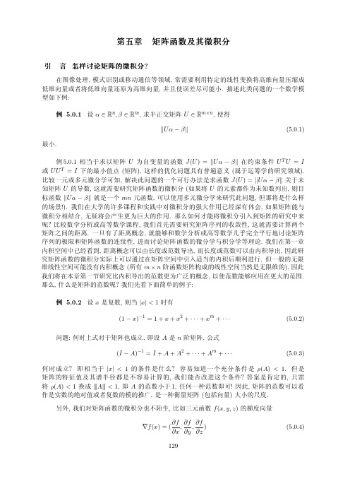
1/p |xj + yj |p
≤
n j =1
1/p |xj |p
+
n j =1
1/p |yj |p , p ≥ 1. (5.1.1)
130
注 1. 定义 5.1.1 中的字母“l”是序列空间 (对照第二章第六节) 或 Lebesgue 49 空间的统称. 确切地说, 数域 F 上的所有绝对收敛的无穷数列构成的线性空间称为 l1 空间, 绝对平方收敛的无穷数列构成的线性空间称为 l2 空间, 所有有界无穷数列构成的线性空间称为 l∞ 空间, 以及 lp 空间等等. 类似地, 可以定义绝对可积函数空间 L1 , 绝对平方可积函数空间 L2 , 以及 Lp , L∞ 等等. 注 2. 当 0 < p < 1 时, lp 范数仍然满足向量范数的前两个条件, 但不满足三角不等式, 见习题 5. 注 3. 对于 C 或 R 上一般 n 维线性空间 V , 可以通过取 V 的一组基, 然后像例 5.1.2 中一样定义 V 的范数. 注 4. 常将 1- 范数称为 Manhattan (曼哈顿)- 度量, 因为在赋范线性空间中可以由范数自然定义距离, 即 d(x, y ) = ||x − y ||. 请读者在平面上或者空间中画出两点间的距离的示意图. 如果连接两点间的最短曲线称为线段, 请问 1- 范数下的线段是什么? ∞- 范数下的线段是什么? 例 5.1.3 (各种范数下的单位圆) 下面的图从左至右依次展示了 1- 范数, 普通范数 (欧几里得范数) 和 ∞- 范数下的平面上的单位圆 ( 1 维单位球面): ||x||1 = 1 T 1
49
Henri L´ eon Lebesgue(1875-1941), 法国数学家, 数学上有著名的 Lebesgue 积分.

矩阵微分方程

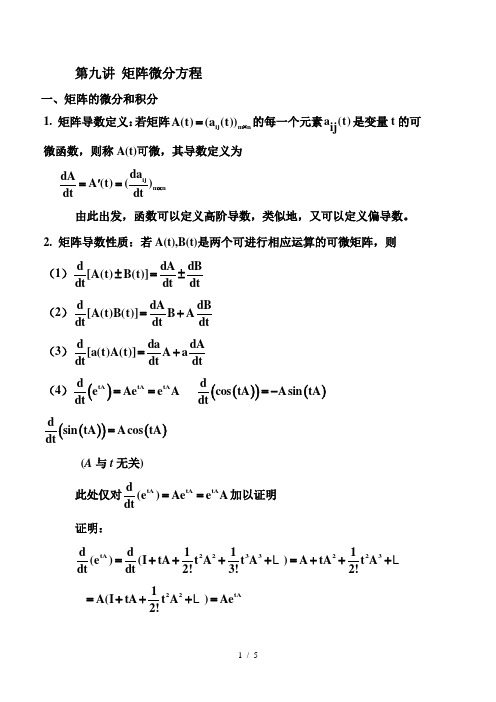
第九讲矩阵微分方程一、矩阵的微分和积分1. 矩阵导数定义：若矩阵ij m n A(t)(a (t))⨯=的每一个元素a (t)ij 是变量t 的可微函数，则称A(t)可微，其导数定义为ij m n da dAA (t)()dt dt⨯'== 由此出发，函数可以定义高阶导数，类似地，又可以定义偏导数。

2. 矩阵导数性质：若A(t),B(t)是两个可进行相应运算的可微矩阵，则（1）d dA dB [A(t)B(t)]dt dt dt ±=±（2）d dA dB[A(t)B(t)]B Adt dt dt=+ （3）d da dA [a(t)A(t)]A adt dt dt =+ （4）()()()()tAtA tA d de Ae e A cos tA Asin tA dtdt ===- ()()()dsin tA Acos tA dt=(A 与t 无关) 此处仅对tAtA tA d (e )Ae e A dt==加以证明证明：tA 2233223d d 111(e )(I tA t A t A )A tA t A dt dt 2!3!2!=++++=+++22tA 1A(I tA t A )Ae 2!=+++=又22tA 1(I tA t A )A e A 2!=+++=3. 矩阵积分定义：若矩阵A(t)(a (t))m n ij =⨯的每个元素ij a (t)都是区间01[t ,t ]上的可积函数，则称A(t)在区间01[t ,t ]上可积，并定义A(t)在01[t ,t ]上的积分为1100ij t t A(t)dt a (t)dt t t m n ⎛⎫=⎰⎰ ⎪⎝⎭⨯ 4. 矩阵积分性质（1）111000t t t t t t [A(t)B(t)]dt A(t)dt B(t)dt ±=±⎰⎰⎰（2）11110000t t t t t t t t [A(t)B]dt A(t)dt B,[AB(t)]dt A B(t)dt ⎛⎫⎛⎫== ⎪ ⎪ ⎪ ⎪⎝⎭⎝⎭⎰⎰⎰⎰（3）t baadA(t )dt A(t),A (t)dt A(b)A(a)dt '''==-⎰⎰二、一阶线性齐次常系数常微分方程组设有一阶线性其次常系数常微分方程组11111221n n 22112222n n n n11n22nn n dx a x (t)a x (t)a x (t)dt dx a x (t)a x (t)a x (t)dtdx a x (t)a x (t)a x (t)dt⎧=+++⎪⎪⎪=+++⎪⎨⎪⎪⎪=+++⎪⎩ 式中t 是自变量，i i x x (t)=是t 的一元函数(i 1,2,,n),=ij a (i,j 1,2,,n)=是常系数。

矩阵函数微积分

dA( X dX
)
A ( xij
) C mpnq
自学:P118
例5,例6
第五节微分方程组的求解
一阶常系数线性齐次微分方程组
dx1
dt dx2 dt
a11x1 a12 x2 a1n xn a21x1 a22 x2 a2n xn
dxn dt
an1x1 an2 x2
ann xn
由函数对矩阵导数的定义可得：
T
df dX
f x1
,
f x2
,,
f xn
df dX T
f x1
,
f x2
,,
f xn
自学:P116 例2,例3,例4
矩阵值函数对矩阵的导数
设 A( X ) ( flk ( X )) Cmn , X (xij ) C pq ,
定义函数矩阵 A(X ) 对矩阵X的导数为：
用拉氏变换求解微分方程组
dx
dt
Ax(t)
x(0) x0
记 X (s) L[(x(t)] , 在微分方程两边取拉氏变换：
L[(x(t)] L[ Ax(t)]
微分性质可得 sX (s) x(0) AX (s)
于是 (sI A)X (s) x(0) 从而 X (s) (sI A)1 x(0)
dt
dt
eAt ( dX AX ) dt
eAt F (t)
在 0,t 上对上式积分得：
d eAt X t eAt Ft
dt
0t
d ds
[e
As
X
(s)]ds
0t
e
As
F
(s)ds
即
eAt X (t) X (0) t eAs F (s)ds 0

矩阵微积分规则

矩阵微积分规则摘要：1.矩阵微积分的概念与基本原理2.矩阵微积分的运算方法3.矩阵微积分在实际问题中的应用正文：矩阵微积分是一种应用于多元函数微分和线性变换的数学工具，它是微积分学在向量空间和矩阵运算中的拓展。

矩阵微积分不仅具有传统微积分的基本原理，还具有独特的运算方法和应用领域。

一、矩阵微积分的概念与基本原理矩阵微积分的概念来源于矩阵运算与多元函数微分的结合。

矩阵微积分的基本原理包括以下几个方面：1.矩阵的导数：设A 是一个m×n 矩阵，其元素为aij，那么A 的导数是一个同样大小的矩阵，记作A"。

A"的元素为a"ij=aij/xk，其中k 为变量。

2.矩阵的梯度：矩阵的梯度是矩阵导数的特例，表示一个标量函数在向量空间中的梯度。

设f(A) 为矩阵A 的某个函数，那么矩阵A 的梯度是一个列向量，其元素为f"(A)·A"，其中f"(A) 表示函数f(A) 的梯度。

3.矩阵的链式法则：矩阵微积分的链式法则与传统微积分的链式法则类似，表示复合函数的导数。

设f(A) 和g(A) 是两个矩阵函数，那么(f(g(A)))"=f"(g(A))·g"(A)。

二、矩阵微积分的运算方法矩阵微积分的运算方法主要包括以下几个方面：1.矩阵乘法：矩阵乘法是矩阵微积分的基础运算，表示两个矩阵之间的乘积。

设A 和B 是两个m×n 矩阵，那么AB 是一个m×n 矩阵，其元素为(AB)ij=aik·bkj。

2.矩阵求导：矩阵求导是矩阵微积分的关键运算，表示矩阵元素的导数。

根据矩阵导数的定义，可以求得任意矩阵A 的导数A"。

3.矩阵求梯度：矩阵求梯度是矩阵微积分的另一个重要运算，表示标量函数在向量空间中的梯度。

根据矩阵梯度的定义，可以求得任意矩阵A 的梯度。

三、矩阵微积分在实际问题中的应用矩阵微积分在实际问题中有广泛的应用，例如在线性代数、优化理论、机器学习等领域。

第八章矩阵微积分

第八章矩阵微积分§8.1 矩阵的Kronecker 积矩阵的Kronecker 积对参与运算的矩阵没有任何限制，在矩阵的理论研究和计算方法中都有十分重要的应用，尤其是在矩阵代数方程求解和矩阵微分等运算中使得计算更加简洁。

本节中，我们将介绍Kronecker 积的定义和基本性质. 8.1.1 Kronecker 积的概念与性质定义1 设矩阵()C m n ij m n a ⨯⨯=∈A ，()C p q ij p q b ⨯⨯=∈B ，则称如下分块矩阵111212122212=C n n mp nq m m mn a B a Ba B a B a Ba B a B a Ba B ⨯⋅⋅⋅⎡⎤⎢⎥⋅⋅⋅⎢⎥⊗∈⎢⎥⋅⋅⋅⋅⋅⋅⋅⋅⋅⋅⋅⋅⎢⎥⋅⋅⋅⎣⎦A B 为矩阵A 与B 的Kronecker 积或称A 与B 的直积，记做⊗A B 。

显然⊗A B 是具有m n ⨯个子块的分块矩阵，每个子块都与矩阵B 同阶，所以⊗A B 是mp nq ⨯阶矩阵。

由定义1显然有矩阵B 与矩阵A 的Kronecker 积为111212122212=C q q pm qn p p pq b A b A b A b A b A b A b A b A b A ⨯⋅⋅⋅⎡⎤⎢⎥⋅⋅⋅⎢⎥⊗∈⎢⎥⋅⋅⋅⋅⋅⋅⋅⋅⋅⋅⋅⋅⎢⎥⋅⋅⋅⎢⎥⎣⎦B A所以，矩阵的Kronecker 积不满足交换律，即一般情况下，⊗≠⊗A B B A 。

例1 设10234,01567⎡⎤⎡⎤==⎢⎥⎢⎥⎣⎦⎣⎦A B ，则 2340001056700001000234000567⎡⎤⎢⎥⋅⋅⎡⎤⎢⎥⊗==⎢⎥⎢⎥⋅⋅⎣⎦⎢⎥⎣⎦B B A B B B203040234020304567506070050607⎛⎫⎪⋅⋅⋅⎛⎫ ⎪⊗== ⎪⎪⋅⋅⋅⎝⎭ ⎪⎝⎭A A AB A A A A 显然，⊗≠⊗A B B A 。

从定义1可以直接给出Kronecker 积简单的运算性质如下。

第五章矩阵函数及其微积分

1≤j ≤n n
|xj |
1/2
(和范数或 l1 范数或 1- 范数 ); |2
1/p
j =1 n j =1 n j =1
|xj |xj
(欧几里得范数或 l2 范数 ); ,p≥1 (H¨ older 范数或 lp 范数或 p- 范数).
|p
显然, 当 n = 1 时, 例 5.1.2 中的所有范数都变成 C 或 R 上的普通范数 (模或绝对值). 容易看出, || · ||1 与 || · ||2 为 H¨ older 范数中取 p = 1 与 p = 2 的情形, 而 || · ||∞ 是 H¨ older 范数当 p → ∞ 的极限情形. 直接验证可知 (见习题 3 ), || · ||∞ 满足定义 5.1.1 的 3 个条件, 因而为 V 上的向量范数. lp 范数 (p ≥ 1) 显然满足定义中的条件 (1) 和 (2). 为验证条件 (3), 只需应用下列 Minkowski 不等式 (证明见习题 4 ):
n i,j =1 n
1/2 |aij |2 |aij |
i=1 n
=
tr(A∗ A) ( Frobenius 范数或 F- 范数) 极大列和范数极大行和范数
||A||1 = max
1≤j ≤n
||A||∞ = max
1≤i≤n
|aij |
j =1
则不难验证 (见习题 6 ), 它们都是 F n×n 中的范数, 因而 F n×n 成为赋范线性空间.
d d E 1 d −1 d
||x||2 = 1 T 1 '$ −1
E &%
||x||∞ = 1 T 1 −1 −1
E

矩阵中的矩阵微积分

矩阵中的矩阵微积分矩阵微积分是线性代数中的一门重要分支，它将微积分的概念和矩阵运算的技巧相结合，增强了线性代数的理论体系和应用能力。

矩阵微积分研究的是矩阵函数的导数和积分、矩阵微分方程以及相关的数学模型和优化算法等。

本文将从三个方面介绍矩阵微积分的基本概念、应用范围以及研究进展，帮助读者深入了解这门重要课程。

一、矩阵微积分的基本概念矩阵微积分的基本概念包括导数、偏导数、积分、微分方程和泰勒公式等。

其中，矩阵函数的导数定义为极限值，偏导数定义为矩阵函数在某个方向上的变化率，积分定义为矩阵函数的面积或体积，微分方程定义为关系一个或多个未知函数、它们的导数和自变量的方程，泰勒公式定义为用无穷阶导数刻画一个矩阵函数在某个区间内的变化趋势。

这些基本概念构成了矩阵微积分的理论基础，为后续的应用提供了强有力的数学支撑。

二、矩阵微积分的应用范围矩阵微积分的应用范围广泛，涵盖了许多不同的学科领域，例如物理学、工程学、计算机科学、金融等。

其中，最为常见的应用是通过矩阵微积分来解决优化问题。

优化问题是指在满足一定约束条件的前提下，使某一目标函数达到最优值的问题。

有了矩阵微积分的支持，我们可以通过求解函数的导数来确定函数的最大值和最小值，从而解决一系列优化问题，例如线性规划、非线性规划、整数规划等。

此外，矩阵微积分还可以用来构建回归分析、时间序列分析、图像处理等各种数学模型，为现代科技的发展提供技术支持。

三、矩阵微积分的研究进展矩阵微积分的研究进展主要体现在以下几个方面：矩阵微积分与偏微分方程的联系、矩阵微积分和概率统计的关系、矩阵微积分在机器学习中的应用等。

其中，矩阵微积分和偏微分方程的联系是一个经典的数学问题，在很多实际问题中都有广泛应用。

数值分析的技术进步，使得矩阵微积分和偏微分方程的求解更加高效和精确。

矩阵微积分和概率统计的关系也是一个热门研究领域，它在矩阵统计、贝叶斯统计、贝尔曼方程等方面都有广泛应用。

矩阵微积分在机器学习中的应用则是当前研究热点之一，它涉及到最小二乘法、核方法、降维等多个方面，为机器学习领域的发展提供了重要的数学基础和算法支持。

[全]矩阵求导matrix calculus

矩阵求导matrix calculus
这是机器学习中常用的矩阵求导类型，向量对标量，向量对向量，矩阵对标量的求导还是容易记忆的，在分子布局的情况下，和常见的函数求导公式是类似，如下面三张图所示。

分母布局一般是分子布局的转置(但不全是)
我这里主要想讲一下标量对标量/向量/矩阵的求导。

矩阵求导是不满足链式法则的，但微分的定义仍然是有用的，我们利用微分和求导的关系，可以构建下面的关系式（注：下面全是针对分子布局来说的）
看不懂？没关系，我们举个例子，对下面的表达式求导，a,b,C都与X无关，C,X表示矩阵，a,b表示向量。

注意到这里的分子部分f是个标量
标量的迹就是它本身，微分号可以提出来：
这里列举了一些迹的相关性质，最后一条比较重要需要用到：
f太复杂了，我们要化简，利用矩阵微分的相关性质
我们利用矩阵微分的乘法性质将其分为了两部分：
接下来应该干什么呢？回到我们的关系式
我们的目标就很明确了，就是要将微分部分dX移到最后一位，这样前面的系数就是我们要求的导数了！
令Y=Xa+b，我们还要将dY表示成dX，同样利用乘法性质
这样上式表示为：
这样导数就是其系数
和wiki matrix calculus上分子布局求导结果是一致的，分母布局就是转置一下
总的来说只要分子是个标量，那么操作是类似的，无论分母是向量还是矩阵。

1、下载文档前请自行甄别文档内容的完整性，平台不提供额外的编辑、内容补充、找答案等附加服务。
2、"仅部分预览"的文档,不可在线预览部分如存在完整性等问题,可反馈申请退款(可完整预览的文档不适用该条件!)。
3、如文档侵犯您的权益，请联系客服反馈,我们会尽快为您处理(人工客服工作时间：9:00-18:30)。

Matrix Diﬀerentiation
( and some other stuﬀ ) Randal J. Barnes Department of Civil Engineering, University of Minnesota Minneapolis, Minnesota, USA
1
Introduction
n
(11)
(12)
cij =
k=1Biblioteka aik bkj(13)
By deﬁnition, the typical element of CT , say dij , is given by
n
dij = cji =
k=1
ajk bki
(14)
Hence, CT = BT AT q.e.d. Proposition 3 Let A and B be n × n and invertible matrices. Let the product AB be given by C = AB (16) then C−1 = B−1 A−1 Proof: CB−1 A−1 = ABB−1 A−1 = I q.e.d. (18) (17) (15)
where B is m1 × n1 , E is m2 × n2 , C is m1 × n2 , D is m2 × n1 , m1 + m2 = m, and n1 + n2 = n. The above is said to be a partition of the matrix A.
1
Much of the material in this section is extracted directly from Dhrymes (1978, Section 2.7).
3
Matrix Multiplication
C = AB (3)
Deﬁnition 3 Let A be m × n, and B be n × p, and let the product AB be
then C is a m × p matrix, with element (i, j) given by
2
CE 8361
Spring 2006
Proposition 2 Let A be m × n, and B be n × p, and let the product AB be C = AB then CT = BT AT Proof: The typical element of C is given by
3
CE 8361
Spring 2006
Proposition 4 Let A be a square, nonsingular matrix of order m. Partition A as A= A11 A12 A21 A22 (20)
so that A11 is a nonsingular matrix of order m1 , A22 is a nonsingular matrix of order m2 , and m1 + m2 = m. Then A
(8)
for all i = 1, 2, . . . , n. Finally, the scalar resulting from the product α = yT Ax is given by
m n
(9)
α=
j=1 k=1
ajk yj xk
(10)
Proof: These are merely direct applications of Deﬁnition 3. q.e.d.
n
cij =
k=1
aik bkj
(4)
for all i = 1, 2, . . . , m,
j = 1, 2, . . . , p.
Proposition 1 Let A be m × n, and x be n × 1, then the typical element of the product z = Ax is given by
−1
=
1 A11 − A12 A− 22 A21
−1 −1
1 −1 −A− 11 A12 A22 − A21 A11 A12 1 A22 − A21 A− 11 A12 −1
−1
1 −1 −A− 22 A21 A11 − A12 A22 A21
(21)
Proof: Direct multiplication of the proposed A−1 and A yields A−1 A = I q.e.d. (22)
5
Matrix Diﬀerentiation
In the following discussion I will diﬀerentiate matrix quantities with respect to the elements of the referenced matrices. Although no new concept is required to carry out such operations, the element-by-element calculations involve cumbersome manipulations and, thus, it is useful to derive the necessary results and have them readily available 2 . Convention 3 Let y = ψ(x), where y is an m-element vector, and x is an n-element ∂y ∂y1 1 ··· ∂x1 ∂x ∂y2 ∂y2 2 ··· ∂y ∂x1 ∂x2 = . . . ∂x . . .
m× n
and n columns. A superscript T denotes the matrix transpose operation; for example, AT denotes the transpose of A. Similarly, if A has an inverse it will be denoted by A−1 . The determinant of A will be denoted by either |A| or det(A). Similarly, the rank of a matrix A is denoted by rank(A). An identity matrix will be denoted by I, and 0 will denote a null matrix.
1
CE 8361
Spring 2006
Convention 2 When it is useful to explicitly attach the matrix dimensions to the symbolic notation, I will use an underscript. For example, A , indicates a known, multi-column matrix with m rows
n
(5)
zi =
k=1
aik xk
(6)
for all i = 1, 2, . . . , m. Similarly, let y be m × 1, then the typical element of the product zT = yT A is given by
n
(7)
zi =
k=1
aki yk
Throughout this presentation I have chosen to use a symbolic matrix notation. This choice was not made lightly. I am a strong advocate of index notation, when appropriate. For example, index notation greatly simpliﬁes the presentation and manipulation of diﬀerential geometry. As a rule-of-thumb, if your work is going to primarily involve diﬀerentiation with respect to the spatial coordinates, then index notation is almost surely the appropriate choice. In the present case, however, I will be manipulating large systems of equations in which the matrix calculus is relatively simply while the matrix algebra and matrix arithmetic is messy and more involved. Thus, I have chosen to use symbolic notation.
2
Notation and Nomenclature
Deﬁnition 1 Let aij ∈ R, i = 1, 2, . . . , m, j = 1, 2, . . . , n. Then the ordered rectangular array a11 a12 · · · a1n a21 a22 · · · a2n A= (1) . . . . . . . . . am1 am2 · · · amn is said to be a real matrix of dimension m × n. When writing a matrix I will occasionally write down its typical element as well as its dimension. Thus, A = [aij ] , i = 1, 2, . . . , m; j = 1, 2, . . . , n, (2) denotes a matrix with m rows and n columns, whose typical element is aij . Note, the ﬁrst subscript locates the row in which the typical element lies while the second subscript locates the column. For example, ajk denotes the element lying in the jth row and kth column of the matrix A. Deﬁnition 2 A vector is a matrix with only one column. Thus, all vectors are inherently column vectors. Convention 1 Multi-column matrices are denoted by boldface uppercase letters: for example, A, B, X. Vectors (single-column matrices) are denoted by boldfaced lowercase letters: for example, a, b, x. I will attempt to use letters from the beginning of the alphabet to designate known matrices, and letters from the end of the alphabet for unknown or variable matrices.

矩阵微积分MatrixCalculus

Matrix Calculus

微积分与矩阵

机器学习算法原理——矩阵微积分，构建你的“黑客帝国”

矩阵微积分基础知识

矩阵微积分

Matrix Calculate

微积分与矩阵

MATRIX CALCULATION

矩阵的微分与积分

第五章 矩阵函数及其微积分

矩阵微分方程

矩阵函数微积分

矩阵微积分规则

第八章 矩阵微积分

第五章 矩阵函数及其微积分

矩阵中的矩阵微积分

[全]矩阵求导matrix calculus

第五章矩阵函数及其微积分

第八章矩阵微积分

第五章矩阵函数及其微积分