CHAPTER7.4
第七章 图论
12
7.1 图及相关概念
7.1.5 子图
Graphs
图论
定义7-1.8 给定图G1=<V1,E1>和G2=<V2,E2> , (1)若V1V2 ,E1E2 ,则称G1为G2的子图。 (2)若V1=V2 ,E1E2 ,则称G1为G2的生成子图。
上图中G1和G2都是G的子图,
但只有G2是G的生成子图。
chapter7
18
7.1 图及相关概念
7.1.6 图的同构
Graphs
图论
【例4】 设G1,G2,G3,G4均是4阶3条边的无向简单图,则
它们之间至少有几个是同构的? 解:由下图可知,4阶3条边非同构的无向简单图共有3个, 因此G1,G2,G3,G4中至少有2个是同构的。
4/16/2014 5:10 PM
4/16/2014 5:10 PM chapter7 10
7.1 图及相关概念
7.1.3 完全图
Graphs
图论
【例2】证明在 n(n≥2 )个人的团体中,总有两个人在 此团体中恰好有相同个数的朋友。 分析 :以结点代表人,二人若是朋友,则在结点间连上一 证明:用反证法。 条边,这样可得无向简单图G,每个人的朋友数即该结点 设 G 中各顶点的度数均不相同,则度数列为 0 , 1 , 2 , …, 的度数,于是问题转化为: n 阶无向简单图 G中必有两个 n-1 ,说明图中有孤立顶点,与有 n-1 度顶点相矛盾(因 顶点的度数相同。 为是简单图),所以必有两个顶点的度数相同。
vV1
deg(v) deg(v) deg(v) 2 | E |
vV2 vV
由于 deg( v) 是偶数之和,必为偶数,
vV1
形式语言与自动机Chapter7练习参考解答
Chapter 7 练习参考解答Exercise 7.1.3 从以下文法出发:S → 0A0 | 1B1 | BBA → CB → S | AC → S | εa) 有没有无用符号?如果有的话去除它们。
b) 去除ε-产生式。
c) 去除单位产生式。
d) 把该文发转化为乔姆斯基范式。
参考解答:a)没有无用符.b) 所有符号S,A,B,C都是可致空的,消去ε-产生式后得到新的一组产生式:S → 0A0 | 1B1 | BB | B | 00 | 11A → CB → S | AC → Sc) 单元偶对包括:(A,A),(B,B),(C,C),(S,S),(A,C),(A,S),(A,B),(B,A),(B,C),(B,S),(C,A),(C,B),(C,S),(S,A),(S,B),(S,C),消去单元产生式后得到新的一组产生式S → 0A0 | 1B1 | BB | B | 00 | 11A → CB → S | AC → SS → 0A0 | 1B1 | BB | 00 | 11A → 0A0 | 1B1 | BB | 00 | 11B → 0A0 | 1B1 | BB | 00 | 11C → 0A0 | 1B1 | BB | 00 | 11d)先消去无用符号C,得到新的一组产生式:S → 0A0 | 1B1 | BB | 00 | 11A → 0A0 | 1B1 | BB | 00 | 11B → 0A0 | 1B1 | BB | 00 | 11引入非终结符C,D,增加产生式C → 0和D → 1,得到新的一组产生式:S → CAC | DBD | BB | CC | DDA → CAC | DBD | BB | CC | DDB → CAC | DBD | BB | CC | DDC → 0D → 1引入非终结符E,F,增加产生式E → CA和F → DB,得到满足Chomsky范式的一组产生式:S → EC | FD | BB | CC | DDA → EC | FD | BB | CC | DDB → EC | FD | BB | CC | DDE → CAF → DBC → 0D → 1Exercise 7.2.1(b)用CFL泵引理来证明下面的语言都不是上下文无关的:b) {a n b n c i | i ≤n}。
简明英语语言学教程 Chapter 7

• Children's acquisition of language is quickly and effortlessly. It seems that their acquisition process is simple and straightforward . • In the learning of language , children's grammar is never exactly like that of the adult community . • Language has a lot of dialects and many individual styles.The features of these grammers may the merge(合并)----lead to certain rules of language may be simplified or overgeneralized.
• The reasons for some changes are relatively obvious. For example, the rapid development of science and technology has led to the creation of many new words.Such as bullet train ,laser printer,CD-ROM , laptop computer, iphone. • Social and political changes and political needs have supplied the English vocabulary with a great number of new words and expressions: shuttle diplomacy,mini-summit,jungle war,Scientific Outlook on Development • Some other words have also changed as women have taken up activities formerly reserved for men .
Hierarchical cluster analysis

Chapter 7Hierarchical cluster analysisIn Part 2 (Chapters 4 to 6) we defined several different ways of measuring distance (or dissimilarity as the case may be) between the rows or between the columns of the data matrix, depending on the measurement scale of the observations. As we remarked before, this process often generates tables of distances with even more numbers than the original data, but we will show now how this in fact simplifies our understanding of the data. Distances between objects can be visualized in many simple and evocative ways. In this chapter we shall consider a graphical representation of a matrix of distances which is perhaps the easiest to understand – a dendrogram, or tree – where the objects are joined together in a hierarchical fashion from the closest, that is most similar, to the furthest apart, that is the most different. The method of hierarchical cluster analysis is best explained by describing the algorithm, or set of instructions, which creates the dendrogram results. In this chapter we demonstrate hierarchical clustering on a small example and then list the different variants of the method that are possible.ContentsThe algorithm for hierarchical clusteringCutting the treeMaximum, minimum and average clusteringValidity of the clustersClustering correlationsClustering a larger data setThe algorithm for hierarchical clusteringAs an example we shall consider again the small data set in Exhibit 5.6: seven samples on which 10 species are indicated as being present or absent. In Chapter 5 we discussed two of the many dissimilarity coefficients that are possible to define between the samples: the first based on the matching coefficient and the second based on the Jaccard index. The latter index counts the number of ‘mismatches’ between two samples after eliminating the species that do not occur in either of the pair. Exhibit 7.1 shows the complete table of inter-sample dissimilarities based on the Jaccard index.Exhibit 7.1 Dissimilarities, based on the Jaccard index, between all pairs ofseven samples in Exhibit 5.6. For example, between the first two samples, A andB, there are 8 species that occur in on or the other, of which 4 are matched and 4are mismatched – the proportion of mismatches is 4/8 = 0.5. Both the lower andupper triangles of this symmetric dissimilarity matrix are shown here (the lowertriangle is outlined as in previous tables of this type.samples A B C D E F GA00.50000.4286 1.00000.25000.62500.3750B0.500000.71430.83330.66670.20000.7778C0.42860.71430 1.00000.42860.66670.3333D 1.00000.8333 1.00000 1.00000.80000.8571E0.25000.66670.4286 1.000000.77780.3750F0.62500.20000.66670.80000.777800.7500G0.37500.77780.33330.85710.37500.75000The first step in the hierarchical clustering process is to look for the pair of samples that are the most similar, that is are the closest in the sense of having the lowest dissimilarity – this is the pair B and F, with dissimilarity equal to 0.2000. These two samples are then joined at a level of 0.2000 in the first step of the dendrogram, or clustering tree (see the first diagram of Exhibit 7.3, and the vertical scale of 0 to 1 which calibrates the level of clustering). The point at which they are joined is called a node.We are basically going to keep repeating this step, but the only problem is how to calculated the dissimilarity between the merged pair (B,F) and the other samples. This decision determines what type of hierarchical clustering we intend to perform, and there are several choices. For the moment, we choose one of the most popular ones, called the maximum, or complete linkage, method: the dissimilarity between the merged pair and the others will be the maximum of the pair of dissimilarities in each case. For example, the dissimilarity between B and A is 0.5000, while the dissimilarity between F and A is 0.6250. hence we choose the maximum of the two, 0.6250, to quantify the dissimilarity between (B,F) and A. Continuing in this way we obtain a new dissimilarity matrix Exhibit 7.2.Exhibit 7.2 Dissimilarities calculated after B and F are merged, using the‘maximum’ method to recomputed the values in the row and column labelled(B,F).samples A(B,F)C D E GA00.62500.4286 1.00000.25000.3750(B,F)0.625000.71430.83330.77780.7778C0.42860.71430 1.00000.42860.3333D 1.00000.8333 1.00000 1.00000.8571E0.25000.77780.4286 1.000000.3750G0.37500.77780.33330.85710.37500Exhibit 7.3 First two steps of hierarchical clustering of Exhibit 7.1, using the ‘maximum’ (or ‘complete linkage’) method.The process is now repeated: find the smallest dissimilarity in Exhibit 7.2, which is 0.2500 for samplesA and E , and then cluster these at a level of 0.25, as shown in the second figure of Exhibit 7.3. Then recomputed the dissimilarities between the merged pair (A ,E ) and the rest to obtain Exhibit 7.4. For example, the dissimilarity between (A ,E ) and (B ,F ) is the maximum of 0.6250 (A to (B ,F )) and 0.7778 (E to (B ,F )).Exhibit 7.4 Dissimilarities calculated after A and E are merged, using the ‘maximum’ method to recomputed the values in the row and column labelled (A ,E ).samples(A,E)(B,F)CDG(A,E)00.77780.4286 1.00000.3750(B,F)0.777800.71430.83330.7778C 0.42860.71430 1.00000.3333D1.00000.8333 1.000000.8571G 0.37500.77780.33330.85710In the next step the lowest dissimilarity in Exhibit 7.4 is 0.3333, for C and G – these are merged, as shown in the first diagram of Exhibit 7.6, to obtain Exhibit 7.5. Now the smallest dissimilarity is 0.4286, between the pair (A ,E ) and (B ,G ), and they are shown merged in the second diagram of Exhibit 7.6. Exhibit 7.7 shows the last two dissimilarity matrices in this process, and Exhibit 7.8 the final two steps of the construction of the dendrogram, also called a binary tree because at each step two objects (or clusters of objects) are merged. Because there are 7 objects to be clustered, there are 6 steps in the sequential process (i.e., one less) to arrive at the final tree where all objects are in a single cluster. For botanists that may be reading this: this is an upside-down tree, of course!1.00.50.0B F B F A E1.00.50.0Exhibit 7.5 Dissimilarities calculated after C and G are merged, using the‘maximum’ method to recomputed the values in the row and column labelled (C,G).samples(A,E)(B,F)(C,G)D(A,E)00.77780.4286 1.0000(B,F)0.777800.77780.8333(C,G)0.42860.77780 1.0000D 1.00000.8333 1.00000Exhibit 7.6 The third and fourth steps of hierarchical clustering of Exhibit 7.1, using the ‘maximum’ (or ‘complete linkage’) method. The point at which objects (or clusters of objects) are joined is called a node.Exhibit 7.7 Dissimilarities calculated after C and G are merged, using the‘maximum’ method to recomputed the values in the row and column labelled (C,G).samples(A,E,C,G)(B,F)D samples(A,E,C,G,B,F)D (A,E,C,G)00.7778 1.0000(A,E,C,G,B,F)0 1.0000 (B,F)0.777800.8333D 1.00000D 1.00000.83330B F A EC G1.00.50.0B F A EC G1.00.50.0Exhibit 7.8 The fifth and sixth steps of hierarchical clustering of Exhibit 7.1, using the ‘maximum’ (or ‘complete linkage’) method. The dendrogram on the right is the final result of the cluster analysis. In the clustering of n objects, there are n–1 nodes (i.e. 6 nodes in this case).Cutting the treeThe final dendrogram on the right of Exhibit 7.8 is a compact visualization of the dissimilarity matrix in Exhibit 7.1, based on the presence-absence data of Exhibit 5.6. Interpretation of the structure of data is made much easier now – we can see that there are three pairs of samples that are fairly close, two of these pairs ((A,E) and (C,G)) are in turn close to each other, while the single sample D separates itself entirely from all the others. Because we used the ‘maximum’ method, all samples clustered below a particular level of dissimilarity will have inter-sample dissimilarities less than that level. For example, 0.5 is the point at which samples are exactly as similar to one another as they are dissimilar, so if we look at the clusters of samples below 0.5 – i.e., (B,F), (A,E,C,G) and (D) – then within each cluster the samples have more than 50% similarity, in other words more than 50% co-presences of species. The level of 0.5 also happens to coincide in the final dendrogram with a large jump in the clustering levels: the node where (A,E) and (C,G) are clustered is at level of 0.4286, while the next node where (B,F) is merged is at a level of 0.7778. This is thus a very convenient level to cut the tree. If the branches are cut at 0.5, we are left with the three clusters of samples (B,F), (A,E,C,G) and (D), which can be labelled types 1, 2 and 3 respectively. In other words, we have created a categorical variable, with three categories, and the samples are categorized as follows:A B C D E F G2 1 23 2 1 2Checking back to Chapter 2, this is exactly the objective which we described in the lower right hand corner of the multivariate analysis scheme (Exhibit 2.2) – to reveal a categorical variable which underlies the structure of a data set.B F A EC G1.00.50.0B F A EC G D1.00.50.0Maximum, minimum and average clusteringThe crucial choice when deciding on a cluster analysis algorithm is to decide how to quantify dissimilarities between two clusters. The algorithm described above was characterized by the fact that at each step, when updating the matrix of dissimilarities, the maximum of the between-cluster dissimilarities was chosen. This is also known as complete linkage cluster analysis, because a cluster is formed when all the dissimilarities (‘links’) between pairs of objects in the cluster are less then a particular level. There are several alternatives to complete linkage as a clustering criterion, and we only discuss two of these: minimum and average clustering.The ‘minimum’ method goes to the other extreme and forms a cluster when only one pair of dissimilarities (not all) is less than a particular level – this is known as single linkage cluster analysis. So at every updating step we choose the minimum of the two distances and two clusters of objects can be merged when there is a single close link between them, irrespective of the other inter-object distances. In general, this is not a suitable choice for most applications, because it can lead to clusters that are quite heterogeneous internally, and the usual object of clustering is to obtain homogeneous clusters.The ‘average’ method is an attractive compromise where dissimilarities are averaged at each step, hence the name average linkage cluster analysis. For example, in Exhibit 7.1 the first step of all types of cluster analysis would merge B and F. But then calculating the dissimilarity between A, for example, and (B,F) is where the methods distinguish themselves. The dissimilarity between A and B is 0.5000, and between A and F it is 0.6250. Complete linkage chooses the maximum: 0.6250; single linkage chooses the minimum: 0.5000; while average linkage chooses the average: (0.5000+0.6250)/2 = 0.5625.Validity of the clustersIf a cluster analysis is performed on a data matrix, a set of clusters can always be obtained, even if there is no actual grouping of the objects, in this case the samples. So how can we evaluate whether the three clusters in this example are not just any old three groups which we would have obtained on random data with no structure? There is a vast literature on validity of clusters (we give some references in the Bibliography, Appendix E) and here we shall explain one approach based on permutation testing. In our example, the three clusters were formed so that internally in each cluster formed by more than one sample the between-sample dissimilarities were all less than 0.5000. In fact, if we look.at the result in the right hand picture of Exhibit 7.8, the cutpoint for three clusters can be brought down to the level of 0.4286, where (A,E) and (C,G) joined together. As in all statistical considerations of significance, we ask whether this is an unusual result or whether it could have arisen merely by chance. To answer this question we need an idea of what might have happened in chance results, so that we can judge our actual finding. This so-called “null distribution” can be generated through permuting the data in some reasonable way, evaluating the statistic of interest, and doing this many times (or for all permutations if this is feasible computationally) to obtain a distribution of the statistic. The statistic of interest could be that value at which the three clusters are formed, but we need to choose carefullyhow we perform the permutations, and this depends on how the data were collected. We consider two possible assumptions, and show how different the results can be.The first assumption is that the column totals of Table Exhibit 5.6 are fixed; that is, that the 10 species are present, respectively, 3 times in the 7 samples, 6 times, 4 times, 3 times and so on. Then the permutation involved would be to simply randomly shuffle the zeros and ones in each column to obtain a new presence-absence matrix with exactly the same column totals as before. Performing the compete linkage hierarchical clustering on this matrix leads to that value where the three cluster solution is achieved, and becomes one observation of the null permutation distribution. We did this 9999 times, and along with our actual observed value of 0.4286, the 10000 values are graphed in Exhibit 7.9 (we show it as a horizontal bar chart because there are only 15 different values observed of this value, shown here with their frequencies). The value we actually observed is one of the smallest – the number of permuted matrices that generates this value or a lower value is 26 out of 10000, so that in this sense our data are very unusual and the ‘significance’ of the three-cluster solution can be quantified with a p -value of 0.0026. The other 9974 randompermutations all lead to generally higher inter-sample dissimilarities such that the level at which three-cluster solutions are obtained is 0.4444 or higher (0.4444 corresponds to 4 mistmatches out of 9.Exhibit 7.9 Bar chart of the 10000 values of the three-cluster solutions obtained by permuting the columns of the presence-absence data, including the value we observed in the original unpermuted data matrix.The second and alternative possible assumption for the computation of the null distribution could be that the column margins are not fixed, but random; in other words, we relax the fact that there were exactly 3 samples that had species sp1, for example, and assume a binomial distribution for each column, using the observed proportion (3 out of 7 forspecies sp1) and the number of samples (7) as the binomial parameters. Thus there can be 0 up to 7 presences in each column, according to the binomial probabilities for eachspecies. This gives a much wider range of possibilities for the null distribution, and leads us to a different conclusion about our three observed clusters. The permutation distributionlevel frequency0.800020.7778350.75003630.714313600.70001890.666729670.625021990.60008220.571413810.55552070.50004410.444480.4286230.400020.37501is now shown in Exhibit 7.10, and now our observed value of 0.4286 does not look sounusual, since 917 out of 10000 values in the distribution are less than or equal to it, giving an estimated P -value of 0.0917.Exhibit 7.10 Bar chart of the 10000 values of the three-cluster solutionsobtained by generating binomial data in each column of the presence-absence matrix, according to the probability of presence of each species.So, as in many situations in statistics, the result and decision depends on the initialassumptions. Could we have observed the presence of species s1 less or more than 3 times in the 7 samples (and so on for the other species)? In other words, according to thebinomial distribution with n = 7, and p = 3/7, the probabilities of observing k presences of species sp1 (k = 0, 1, …, 7) are:0 1 2 3 4 5 6 7 0.020 0.104 0.235 0.294 0.220 0.099 0.025 0.003If this assumption (and similar ones for the other nine species) is realistic, then the cluster significance is 0.0917. However, if the first assumption is adopted (that is, the probability of observing 3 presences for species s1 is 1 and 0 for other possibilities), then the significance is 0.0028. Our feeling is that perhaps the binomial assumption is more realistic, in which case our cluster solution could be observed in just over 9% of random cases – this gives us an idea of the validity of our results and whether we are dealing with real clusters or not. The value of 9% is a measure of ‘clusteredness’ of our samples in terms of the Jaccard index: the lower this measure, the more they are clustered, and the hoihger the measure, the more the samples lie in a continuum. Lack of evidence oflevel frequency0.875020.857150.8333230.8000500.7778280.75002010.71434850.7000210.666712980.625011710.60008950.571419600.55554680.500022990.44441770.42865670.40001620.37501070.3333640.300010.2857120.250030.20001‘clusteredness’ does not mean that the clustering is not useful: we might want to divide up the space of the data into separate regions, even though the borderlines between them are ‘fuzzy’. And speaking of ‘fuzzy’, there is an alternative form of cluster analysis (fuzzy cluster analysis, not treated specifically in this book) where samples are classified fuzzily into clusters, rather than strictly into one group or another – this idea is similar to the fuzzy coding we described in Chapter 3.Clustering correlations on variablesJust like we clustered samples, so we can cluster variables in terms of their correlations, or distances based on their correlations as described in Chapter 6. The dissimilarity based on the Jaccard index can also be used to measure similarity between species – the index counts the number of samples that have both species of the pair, relative to the number of samples that have at least one of the pair, and the dissimilarity is 1 minus this index.Exhibit 7.11 shows the cluster analyses based on these two alternatives, for the columns of Exhibit 5.6, using the graphical output this time of the R function hclust for hierarchical clustering. The fact that these two trees are so different is no surprise: the first one is based on the correlation coefficient takes into account the co-absences, which strengthens the correlation, while the second does not. Both have the pairs (sp2,sp5) and (sp3,sp8) at zero dissimilarity because these are identically present and absent across the samples. Species sp1 and sp7 are close in terms of correlation, due to co-absences – sp7 only occurs in one sample, sample E , which also has sp1, a species which is absent in four other samples. Notice in Exhibit 7.11(b) how species sp10 and sp1 both join the cluster (sp2,sp5) at the same level (0.5).Exhibit 7.11 Complete linkage cluster analyses of (a) 1–r (1 minus the correlation coefficient between species); (b) Jaccard dissimilarity between species (1 minus the Jaccard similarity index). The R function hclust which calculates the dendrograms places the object (species) labels at a constant distance below its clustering level.(a) (b)s p 1s p 7s p 2s p 5s p 9s p 3s p 8s p 6s p 4s p 100.00.51.01.52.0H e i g h ts p 4s p 6s p 10s p 1s p 2s p 5s p 7s p 9s p 3s p 80.00.20.40.60.81.0H e i g h tClustering a larger data setThe more objects there are to cluster, the more complex becomes the result. In Exhibit 4.5 we showed part of the matrix of standardized Euclidean distances between the 30 sites of Exhibit 1.1, and Exhibit 7.12 shows the hierarchical clustering of this distance matrix, using compete linkage. There are two obvious places where we can cut the tree, at about level 3.4, which gives four clusters, or about 2.7, which gives six clusters. To get an ideaExhibit 7.12 Complete linkage cluster analyses of the standardized Euclidean distances of Exhibit 4.5.of the ‘clusteredness’ of these data, we performed a permutation test similar to the one described above, where the data are randomly permuted within their columns and the cluster analysis repeated each time to obtain 6 clusters. The permutation distribution of levels at which 6 clusters are formed is shown in Exhibit 7.13 – the observed value in Exhibit 7.12 (i.e., where (s2,s14) joins (s25,s23,s30,s12,s16,s27)) is 2.357, which is clearly not an unusual value. The estimated p -value according to the proportion of the distribution to the left of 2.357 in Exhibit 7.13 is p = 0.3388, so we conclude that these samples do not have a non-random cluster structure – they form more of a continuum, which will be the subject of Chapter 9.s s 2s 23s 3016s 27s s s 2 4 classes6 classes7-11Exhibit 7.13 Estimated permutation distribution for the level at which 6clusters are formed in the cluster analysis of Exhibit 7.12, showing the valueactually observed. Of the 10000 permutations, including the observed value,3388 are less than or equal to the observed value, giving an estimated p -valuefor clusteredness of 0.3388.SUMMARY: Hierarchical cluster analysis1. Hierarchical cluster analysis of n objects is defined by a stepwise algorithm whichmerges two objects at each step, the two which have the least dissimilarity.2. Dissimilarities between clusters of objects can be defined in several ways; forexample, the maximum dissimilarity (complete linkage), minimum dissimilarity (single linkage) or average dissimilarity (average linkage).3. Either rows or columns of a matrix can be clustered – in each case we choose theappropriate dissimilarity measure that we prefer.4. The results of a cluster analysis is a binary tree, or dendrogram, with n – 1 nodes. Thebranches of this tree are cut at a level where there is a lot of ‘space’ to cut them, that is where the jump in levels of two consecutive nodes is large.5. A permutation test is possible to validate the chosen number of clusters, that is to seeif there really is a non-random tendency for the objects to group together. 6-clu ster level f r e q u e n c y 2.0 2.5 3.002004006008001000(observed value)。
7.4 Laplace逆变换

解法1: s1 1 和 s2 2 分别是 F (s)est 的1级
和3级极点, 故由计算留数的法则
Res F (s)est ,
1
lim
s1
5s
2 (s
15s 2)3
11
e
st
1 et , 3
Res F (s)est ,
2
1
d2
2!
lim
s2
ds2
5s2
15s s1
11
e
st
孤立奇点,除这些奇点之外, F (s)est 处处解析.
y
+iR
O
x
iR
于是定,理根4.据5 (留数基本定理) 设函数f (z)在区域D
内内包除21π含有i 所限有个i奇 iR孤R F点立(s在奇)e其点std内zs1,部zC2R的, F分,(zs段n)外e光std处滑s处正解向k析n1JR,oCers是d[aFDn(s)est , sk ].
i
n
Res[F (s)est , sk ]
k 1
(t 0)
n
即 f (t)= -1[F(s)] Res[F(s)est , sk ] k 1
证明: 取 R 0 充分大,
使得 s1, s2 , , sn 都在圆弧
CR
CR 和直线 Re s 所围成
的区域内. 因为 est 是全平面
奇点
上的解析函数,因此,s1, s2 , , sn 是 F (s)est 的
s(
s
1
1)2
est
,
est
1
lim
s1
s
et (t 1),
因而,
1
s(s
钢结构连接计算讲解

钢结构设计原理 Design Principles of Steel Structure
7.3.2 对接焊缝的计算
第七章
Chapter 7
连接
Connections
1. 轴心受力的对接焊缝
N lwt
ftw
或
f cw(7.3.1)
lw——焊缝计算长度,
图7.3.5 直对接焊缝连接
t——连接件的较小厚度,对T形接头为腹板的厚度 ;
连接
Connections
(1)焊缝形式:分为对接焊缝和角焊缝。
对接焊缝按受力与焊缝方向分:
1)正对接焊缝(a):作用力方向与焊缝方向正交。 2)斜对接焊缝(b):作用力方向与焊缝方向斜交。
角焊缝按受力与焊缝方向分:
1)正面角焊缝(c) :作用力方向与焊缝长度方向垂直。 2)侧面角焊缝(c) :作用力方向与焊缝长度方向平行。
钢结构设计原理 Design Principles of Steel Structure
(3) 焊缝代号
第七章
Chapter 7
连接
Connections
表7.2.1 焊缝代号
钢结构设计原理 Design Principles of Steel Structure
7.3 对接焊缝的构造和计算
第七章
ftw 185N/mm2
b)最大剪应力
钢结构设计原理 Design Principles of Steel Structure
第七章
Chapter 7
连接
Connections
max
VSx Ixt
550 103 38105104 12
信号与系统chapter 7离散时间信号与系统的Z域分析
由此可见,位移特性Z域表达式中包含了系统的起始条 件,把时域差分方程转换为Z域代数方程,因此,可以方便 求出Z域的零输入响应和两状态响应。
式(7.3)又称为左移序性质,与拉普拉斯变换的时域 微分特性相当。式(7.4)又称右移序性质,与拉普拉斯变 换的时域积分特性相当。
进一步,对于因果序列 x ( n ) , x ( 1 ) 0 ,x ( 2 ) 0 , ,则
Z [nx(n)u(n)]zdd zn∞ 0znx(n)zdd zX(z)
求下列序列的Z变换。
(1) n 2 u ( n )
n(n 1)
(2)
u(n)
解:(1 )Z[n2 u(n)] zd d z 2zz 1 zd d z2 zd d z zz 1
dz
z2 z
z [
]
, z 1
zlnz1 1ln1 zzlnzz1,z1
(2)因为
Z1
u(n 1) , z 1 z 1
根据Z域积分特性,可得
∞1
X(z)
x 1dx∞
1
z dxln ,z1
2
z x1
z x(x1 )
z1
§ 6. 卷积和定理
若 x1(n)u(n) ZX 1(z),z Rx;x2(n)u(n) ZX2(z),z Rx,则 :
第七章 离散时间信号与系统的Z域分析
7.1引言 7.2 Z 变换 7.3 Z 变换的性质 7.4 反变换 7.5离散时间系统的 Z 域分析 7.6离散时间系统的系统函数与系统特性 7.7离散时间系统的模拟
7.1 引 言
按照与连续时间信号与系统相同的分析方法,本章将
讨论离散时间信号与系统的 z 域分析。
§ 4. Z域微分特性
chapter 7 英汉翻译中的词义引申

the news for the next four weeks was never distinct.
在接下来的四个星期里,消息时好时坏,两种 情况不断交替出现,一直没有明朗化。 (see-saw 在英文中本来是“玩跷跷板”之意, 但在这里如果直译,则译文就会不知所云,无 法同后面内容联系起来。因此,这里我们应该 透过原文的现象去抓住原文的精神实质。将 see-sawing 翻译成“不断交替出现”正是抓 住了精神实质。)
3. 由于这部影片造成了排山倒海的影响,它提供了最好 的契机来开始化解种族矛盾,经过相当长的时间使创伤 得以愈合。 (avalanche 的本义为a large mass of snow and ice crashing down the side of a mountain (Longman Dictionary of Contemporary English) avalanche即“雪崩”。该词语的本义是具体的,但在 本例原文中是用于比喻意义。因此在翻译时,我们要透 过现象看本质。在这里,将该词翻译成汉语的“排山倒 海的影响”正是抓住了所描述事件的本质。)
tiger n. 虎 凶汉,暴徒;凶残成性的人 (穿制服的)马夫 [英口](网球比赛的)劲敌 [美](欢呼三声后)加喊的欢呼; 喝采尾声 虎的图象(以虎为标志的组织) 触发器 work like a tiger 生龙活虎地工作 tiger cat 【动】豹猫 three cheers and a tiger 三声欢呼一声吼 How can you catch tiger cubs without entering the tiger's lair? 不入虎穴, 焉得虎子?
计算机导论-第7章-操作系统

Chapter 7 Operating SystemsKnowledge point:7.1. the definition of an operating system7.2. the components of an operating system7.3. Memory Manager7.4. Process manager7.5. deadlockMultiple-Choice Questions:21. is a program that facilitates the execution of other programs.(7.1)a. An operating systemb. Hardwarec. A queued. An application program22. supervises the activity of each component in a computer system. (7.1)a. An operating systemb. Hardwarec. A queued. An application program23. The earliest operating system, called operating systems, only had to ensure thatresources were transferred from one job to the next. (7.1)a. batchb. time-sharingc. personald. parallel24. A operating system is needed for jobs shared between distant connectedcomputers. (7.1)a. batchb. time-sharingc. paralleld. distributed25. Multiprogramming requires a operating system. (7.1)a. batchb. time-sharingc. paralleld. distributed26. DOS is considered a operating system. (7.1)a. batchb. time-sharingc. paralleld. personal27. A system with more than one CPU requires aoperating system. (7.1)a. batchb. time-sharingc. paralleld. distributed28. is multiprogramming with swapping. (7.3)a. Partitioningb. Pagingc. Demand pagingd. Queuing29. is multiprogramming without swapping. (7.3)a. Partitioningb. Pagingc. Demand pagingd. Queuing30. In , only one program can reside in memory for execution. (7.3)a. monoprogrammingb. multiprogrammingc. partitioningd. paging31. is a multiprogramming method in which multiple programs are entirely inmemory with each program occupying a contiguous space. (7.3)a. Partitioningb. Pagingc. Demand pagingd. Demand segmentation32. In paging, a program is divided into equally sized sections called . (7.3)a. pagesb. framesc. segmentsd. partitions33. In , the program can be divided into differently sized sections. (7.3)a. partitioningb. pagingc. demand pagingd. demand segmentation34. In , the program can be divided into equally sized sections called pages, but thepages need not be in memory at the same time for execution. (7.3)a. partitioningb. pagingc. demand pagingd. demand segmentation35. A process in the state can go to either the ready, terminated, or waiting state.(7.4)a. holdb. virtualc. runningd. a and c36. A process in the ready state goes to the running state when . (7.4)a. it enters memoryb. it requires I/Oc. it gets access to the CPUd. it finishes running37. A program becomes a when it is selected by the operating system and broughtto the hold state. (7.4)a. jobb. processc. deadlockd. partition38. Every process is a . (7.4)a. jobb. programc. partitiond. a and b39. The scheduler creates a process from a job and changes a process back to a job.(7.4)a. jobb. processc. virtuald. queue40. The scheduler moves a process from one process state to another. (7.4)a. jobb. processc. virtuald. queue41. To prevent , an operating system can put resource restrictions on processes. (7.5)a. starvationb. synchronizationc. pagingd. deadlock42. can occur if a process has too many resource restrictions. (7.4)a. Starvationb. Synchronizationc. Pagingd. Deadlock43. The manager is responsible for archiving and backup. (7.2)a. memoryb. processc. deviced. file44. The manager is responsible for access to I/O devices. (7.2)a. memoryb. processc. deviced. file45. The job scheduler and the process scheduler are under the control of themanager. (7.4)a. memoryb. processc. deviced. fileReview questions:4. What are the components of an operating system? (7.2)Answer: An operating system includes: Memory Manager, Process Manager, Device Manager and File Manager13. What kinds of states can a process be in? (7.4)Answer: ready state, running state, waiting state.15. If a process is in the running state, what states can it go to next? (7.4) Answer: ready state, waiting state.What’s the definition of an operating system? (7.1)Answer: An operating system is an interface between the hardware of a computer and user(programs or humans) that facilitates the execution of other programs and the access to hardware and software resources.What are the four necessary conditions for deadlock? (7.5)Answer: mutual exclusion, resource holding, no preemption and circular waiting. Exercises:46. A computer has a monoprogramming operating system. If the size of memory is 64 MB and the residing operating system needs 4 MB, what is the maximum size of a program that can be run by this computer? (7.3)Answer:The memory size is 64 MB and the residing operating system needs 4 MB. Then there are 60 (64-4) MB left. So the maximum size of a program that can be run by this computer is 60 MB.47. Redo Exercise 46 if the operating system automatically allocates 10 MB of memory to data. (7.3)Answer:The data take 10 MB. Then there are 50(64-4-10) MB left. So the maximum size of a program that can be run by this computer is 50 MB.48. A monoprogramming operating system runs programs that on average need 10 microseconds access to the CPU and 70 microseconds access to the I/O devices. What percentage of time is the CPU idle? (7.3)Answer:In monoprogramming, when one program is being run, no other program can be executed. That is, when a program accesses I/O devices, CPU is idle. So the percentage of time of the CPU idle is 70/(70+10) = 87.5%.49. A multiprogramming operating system uses an apportioning scheme and divides the 60MB of available memory into four partitions of 10MB, 12MB, 18MB, and 20MB. The first program to be run needs 17MB and occupies the third partition. The second program needs 8MB and occupies the second partition. Finally, the fourth program needs 20MB and occupies the fourth partition. What is the total memory used? What is the total memory wasted? What percentage of memory is wasted? (7.3) Answer: The total memory used is 55.5 MB. The total memory wasted is 4.5 MB. The percentage of memory wasted is 7.5%.51. A multiprogramming operating system uses paging. The available memory is 60 MB divided into 15 pages, each of 4MB. The first program needs 13 MB. The second program needs 12MB. The third program needs 27 MB. How many pages are used by the first program? How many pages are used by the second program? How many pages are used by the third program? How many pages are unused? What is the total memory wasted? What percentage of memory is wasted? (7.3)Answer:Each page is 4MB. The first program needs 13 MB. It is obviously that 4*3<13<4*4. So the first program uses 4 pages and wastes 3(16-3) MB. The second program needs 12 MB. It is obviously that 12=4*3. So the second program uses 3 pages and wastes 0 MB. The third program needs 27 MB. It is obviously that 4*6<27<4*7. So the first program uses 7 pages and wastes 1(28-27) MB. There are 1(15-4-3-7) page unused. There are totally 4(3+0+1) MB memory wasted. The percent of memory wasted is 4/(60-4*1)=7%.53. What is the status of a process in each of the following situations(according to Figure 7.9)?a. The process is using the CPUb. The process has finished printing and needs the attention of the CPU againc.The process has been stopped because its time slot is over.d. The process is reading data from the keyboarde The process is printing data.(7.4)Answer: a)Running state b)Ready state c) Ready state d)Waiting state e)Waiting state。
Ch07Pindyck生产成本

这是机遇本钱 运用者本钱=机遇本钱+经济折旧=利
率(lìlǜ)*资产价值+经济折旧
第二十七页,共84页。
Chapter 7
Cost in the Long Run
User Cost of Capital = Economic Depreciation + (Interest Rate)*(Value of Capital)
Chapter 7
Measuring Cost: Which Costs Matter?
总本钱(běn qián)包括: Fixed Cost固定本钱(běn qián) Does not vary with the level of output 勇于开始,才能找到成功的路 Variable Cost 可变本钱(běn qián) Cost that varies as output varies
Total cost is the vertical
sum of FC
and VC.
200
TC
VC
Variable cost increases with
production and the rate varies with
increasing and decreasing returns.
100 50
cost
Has no alternative use so cost cannot be recovered – opportunity cost is zero
Decision to buy the equipment might
have been good or bad, but now does not
Chapter 7 Maxima and Minima 最大值与最小值

h20 1600 196 20 4.920 3560 meters
2
• The technique is always the same: (a) take the derivative of the equation; (b) set it equal to zero; and (c) use the second derivative test. • The hardest part of these word problems is when you have to set up the equation yourself. The following is a class AP problem:
Chapter 7 Maxima and Minima
7.1 Applied maxima and minima problems 7.2 Curve sketching 7.3 Finding a cusp 7.4 How to find asymptotes
7.1 Applied maxima and minima problems
There are a few exceptions to every rule. This rule is no different.
• If the derivative of a function is zero at a certain point, it is usually a maximum or minimum-but not always.
c
• If a function has a critical velue at x c , then that value is a f c 0 relative maximum if and it is a relative minimum if
伍德里奇计量经济学第六版答案Chapter 7
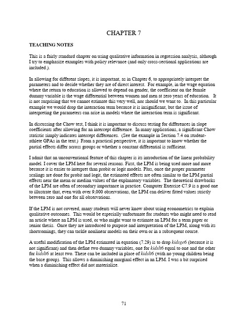
CHAPTER 7TEACHING NOTESThis is a fairly standard chapter on using qualitative information in regression analysis, although I try to emphasize examples with policy relevance (and only cross-sectional applications are included.).In allowing for different slopes, it is important, as in Chapter 6, to appropriately interpret the parameters and to decide whether they are of direct interest. For example, in the wage equation where the return to education is allowed to depend on gender, the coefficient on the female dummy variable is the wage differential between women and men at zero years of education. It is not surprising that we cannot estimate this very well, nor should we want to. In this particular example we would drop the interaction term because it is insignificant, but the issue of interpreting the parameters can arise in models where the interaction term is significant.In discussing the Chow test, I think it is important to discuss testing for differences in slope coefficients after allowing for an intercept difference. In many applications, a significant Chow statistic simply indicates intercept differences. (See the example in Section 7.4 on student-athlete GPAs in the text.) From a practical perspective, it is important to know whether the partial effects differ across groups or whether a constant differential is sufficient.I admit that an unconventional feature of this chapter is its introduction of the linear probability model. I cover the LPM here for several reasons. First, the LPM is being used more and more because it is easier to interpret than probit or logit models. Plus, once the proper parameter scalings are done for probit and logit, the estimated effects are often similar to the LPM partial effects near the mean or median values of the explanatory variables. The theoretical drawbacks of the LPM are often of secondary importance in practice. Computer Exercise C7.9 is a good one to illustrate that, even with over 9,000 observations, the LPM can deliver fitted values strictly between zero and one for all observations.If the LPM is not covered, many students will never know about using econometrics to explain qualitative outcomes. This would be especially unfortunate for students who might need to read an article where an LPM is used, or who might want to estimate an LPM for a term paper or senior thesis. Once they are introduced to purpose and interpretation of the LPM, along with its shortcomings, they can tackle nonlinear models on their own or in a subsequent course.A useful modification of the LPM estimated in equation (7.29) is to drop kidsge6 (because it is not significant) and then define two dummy variables, one for kidslt6 equal to one and the other for kidslt6 at least two. These can be included in place of kidslt6 (with no young children being the base group). This allows a diminishing marginal effect in an LPM. I was a bit surprised when a diminishing effect did not materialize.SOLUTIONS TO PROBLEMS7.1 (i) The coefficient on male is 87.75, so a man is estimated to sleep almost one and one-half hours more per week than a comparable woman. Further, t male = 87.75/34.33 ≈ 2.56, which is close to the 1% critical value against a two-sided alternative (about 2.58). Thus, the evidence for a gender differential is fairly strong.(ii) The t statistic on totwrk is -.163/.018 ≈ -9.06, which is very statistically significant. The coefficient implies that one more hour of work (60 minutes) is associated with .163(60) ≈ 9.8 minutes less sleep.(iii) To obtain 2r R , the R -squared from the restricted regression, we need to estimate themodel without age and age 2. When age and age 2 are both in the model, age has no effect only if the parameters on both terms are zero.7.2 (i) If ∆cigs = 10 then log()bwght ∆ = -.0044(10) = -.044, which means about a 4.4% lower birth weight.(ii) A white child is estimated to weigh about 5.5% more, other factors in the first equation fixed. Further, t white ≈ 4.23, which is well above any commonly used critical value. Thus, the difference between white and nonwhite babies is also statistically significant.(iii) If the mother has one more year of education, the child’s birth weight is estimated to be .3% higher. This is not a huge effect, and the t statistic is only one, so it is not statistically significant.(iv) The two regressions use different sets of observations. The second regression uses fewer observations because motheduc or fatheduc are missing for some observations. We would have to reestimate the first equation (and obtain the R -squared) using the same observations used to estimate the second equation.7.3 (i) The t statistic on hsize 2 is over four in absolute value, so there is very strong evidence that it belongs in the equation. We obtain this by finding the turnaround point; this is the value ofhsize that maximizes ˆsat(other things fixed): 19.3/(2⋅2.19) ≈ 4.41. Because hsize is measured in hundreds, the optimal size of graduating class is about 441.(ii) This is given by the coefficient on female (since black = 0): nonblack females have SAT scores about 45 points lower than nonblack males. The t statistic is about –10.51, so thedifference is very statistically significant. (The very large sample size certainly contributes to the statistical significance.)(iii) Because female = 0, the coefficient on black implies that a black male has an estimated SAT score almost 170 points less than a comparable nonblack male. The t statistic is over 13 in absolute value, so we easily reject the hypothesis that there is no ceteris paribus difference.(iv) We plug in black = 1, female = 1 for black females and black = 0 and female = 1 for nonblack females. The difference is therefore –169.81 + 62.31 = -107.50. Because the estimate depends on two coefficients, we cannot construct a t statistic from the information given. The easiest approach is to define dummy variables for three of the four race/gender categories and choose nonblack females as the base group. We can then obtain the t statistic we want as the coefficient on the black female dummy variable.7.4 (i) The approximate difference is just the coefficient on utility times 100, or –28.3%. The t statistic is -.283/.099 ≈ -2.86, which is very statistically significant.(ii) 100⋅[exp(-.283) – 1) ≈ -24.7%, and so the estimate is somewhat smaller in magnitude.(iii) The proportionate difference is .181 - .158 = .023, or about 2.3%. One equation that can be estimated to obtain the standard error of this difference islog(salary ) = 0β + 1βlog(sales ) + 2βroe + 1δconsprod + 2δutility +3δtrans + u ,where trans is a dummy variable for the transportation industry. Now, the base group is finance , and so the coefficient 1δ directly measures the difference between the consumer products and finance industries, and we can use the t statistic on consprod .7.5 (i) Following the hint, colGPA = 0ˆβ + 0ˆδ(1 – noPC ) + 1ˆβhsGPA + 2ˆβACT = (0ˆβ + 0ˆδ) - 0ˆδnoPC + 1ˆβhsGPA + 2ˆβACT . For the specific estimates in equation (7.6), 0ˆβ = 1.26 and 0ˆδ = .157, so the new intercept is 1.26 + .157 = 1.417. The coefficient on noPC is –.157.(ii) Nothing happens to the R -squared. Using noPC in place of PC is simply a different way of including the same information on PC ownership.(iii) It makes no sense to include both dummy variables in the regression: we cannot hold noPC fixed while changing PC . We have only two groups based on PC ownership so, in addition to the overall intercept, we need only to include one dummy variable. If we try toinclude both along with an intercept we have perfect multicollinearity (the dummy variable trap).7.6 In Section 3.3 – in particular, in the discussion surrounding Table 3.2 – we discussed how to determine the direction of bias in the OLS estimators when an important variable (ability, in this case) has been omitted from the regression. As we discussed there, Table 3.2 only strictly holds with a single explanatory variable included in the regression, but we often ignore the presence of other independent variables and use this table as a rough guide. (Or, we can use the results of Problem 3.10 for a more precise analysis.) If less able workers are more likely to receivetraining, then train and u are negatively correlated. If we ignore the presence of educ and exper , or at least assume that train and u are negatively correlated after netting out educ and exper , then we can use Table 3.2: the OLS estimator of 1β (with ability in the error term) has a downward bias. Because we think 1β ≥ 0, we are less likely to conclude that the training program waseffective. Intuitively, this makes sense: if those chosen for training had not received training, they would have lowers wages, on average, than the control group.7.7 (i) Write the population model underlying (7.29) asinlf = 0β + 1βnwifeinc + 2βeduc + 3βexper +4βexper 2 + 5βage+ 6βkidslt6 + 7βkidsage6 + u ,plug in inlf = 1 – outlf , and rearrange:1 – outlf = 0β + 1βnwifeinc + 2βeduc + 3βexper +4βexper2 + 5βage+ 6βkidslt6 + 7βkidsage6 + u ,oroutlf = (1 - 0β) - 1βnwifeinc - 2βeduc - 3βexper - 4βexper 2 - 5βage - 6βkidslt6 - 7βkidsage6 - u ,The new error term, -u , has the same properties as u . From this we see that if we regress outlf on all of the independent variables in (7.29), the new intercept is 1 - .586 = .414 and each slope coefficient takes on the opposite sign from when inlf is the dependent variable. For example, the new coefficient on educ is -.038 while the new coefficient on kidslt6 is .262.(ii) The standard errors will not change. In the case of the slopes, changing the signs of the estimators does not change their variances, and therefore the standard errors are unchanged (butthe t statistics change sign). Also, Var(1 - 0ˆβ) = Var(0ˆβ), so the standard error of the intercept is the same as before.(iii) We know that changing the units of measurement of independent variables, or entering qualitative information using different sets of dummy variables, does not change the R -squared. But here we are changing the dependent variable. Nevertheless, the R -squareds from the regressions are still the same. To see this, part (i) suggests that the squared residuals will be identical in the two regressions. For each i the error in the equation for outlf i is just the negative of the error in the other equation for inlf i , and the same is true of the residuals. Therefore, the SSRs are the same. Further, in this case, the total sum of squares are the same. For outlf we haveSST = 2211()[(1)(1)]n n i i i i outlf outlf inlf inlf ==-=---∑∑= 2211()()n ni i i i inlf inlf inlf inlf ==-+=-∑∑,which is the SST for inlf . Because R 2 = 1 – SSR/SST, the R -squared is the same in the two regressions.7.8 (i) We want to have a constant semi-elasticity model, so a standard wage equation with marijuana usage included would belog(wage ) = 0β + 1βusage + 2βeduc + 3βexper + 4βexper 2 + 5βfemale + u .Then 100⋅1β is the approximate percentage change in wage when marijuana usage increases byone time per month.(ii) We would add an interaction term in female and usage :log(wage ) = 0β + 1βusage + 2βeduc + 3βexper + 4βexper 2 + 5βfemale+ 6βfemale ⋅usage + u .The null hypothesis that the effect of marijuana usage does not differ by gender is H 0: 6β = 0.(iii) We take the base group to be nonuser. Then we need dummy variables for the other three groups: lghtuser , moduser , and hvyuser . Assuming no interactive effect with gender, the model would belog(wage ) = 0β + 1δlghtuser + 2δmoduser + 3δhvyuser + 2βeduc + 3βexper + 4βexper 2 + 5βfemale + u .(iv) The null hypothesis is H 0: 1δ = 0, 2δ= 0, 3δ = 0, for a total of q = 3 restrictions. If n is the sample size, the df in the unrestricted model – the denominator df in the F distribution – is n – 8. So we would obtain the critical value from the F q ,n -8 distribution.(v) The error term could contain factors, such as family background (including parental history of drug abuse) that could directly affect wages and also be correlated with marijuana usage. We are interested in the effects of a person’s drug usage on his or her wage, so we would like to hold other confounding factors fixed. We could try to collect data on relevant background information.7.9 (i) Plugging in u = 0 and d = 1 gives 10011()()()f z z βδβδ=+++.(ii) Setting **01()()f z f z = gives **010011()()z z βββδβδ+=+++ or *010z δδ=+. Therefore, provided 10δ≠, we have *01/z δδ=-. Clearly, *z is positive if and only if 01/δδ is negative, which means 01 and δδ must have opposite signs.(iii) Using part (ii) we have *.357/.03011.9totcoll == years.(iv) The estimated years of college where women catch up to men is much too high to be practically relevant. While the estimated coefficient on female totcoll ⋅ shows that the gap is reduced at higher levels of college, it is never closed – not even close. In fact, at four years of。
系统辨识(英文版),教材Chapter 7
Non-stationary continuous components
y (t ) − y (t − 1) u (t ) − u (t − 1)
The I/O signals are replaced by their corresponding variations (eventually filtered).
I.D. Landau, G. Zito - "Digital Control Systems" - Chapter 7
8
Over-sampling
Digital anti-aliasing filter For n > 3 a moving-average filter is sufficient
Plant operated in closed loop with excitation added to the controller output
PRBS y0 y1
reference
+
Controller Physical u(t) system
+ output
y(t)
• PRBS superposed to the controller output • Identification of the transfer function between y0 and y
I.D. Landau, G. Zito - "Digital Control Systems" - Chapter 7
Use of a controller with integral action but limited proportional and derivative actions
【13】Chapter7 散列表应用

散列方法的应用
对等网络(P2P)中的应用 对等网络(P2P) 例如,emule软件 例如,emule软件 用散列函数压缩序数索引 信息安全方面的应用 a)攻击路径重构 a)攻击路径重构
• 在路由器上利用散列表记录IP报文头部信息,实现攻击路径的 在路由器上利用散列表记录IP报文头部信息, 报文头部信息 重构,从而追踪到攻击主机的地址。 重构,从而追踪到攻击主机的地址。
LZW压缩 LZW压缩
【LZW编码的原理】 LZW编码的原理 编码的原理】 编码器逐个输入字符并累积一个字符串I 编码器逐个输入字符并累积一个字符串I。 每输入一个字符则串接在I后面,然后在字典中查找I 每输入一个字符则串接在I后面,然后在字典中查找I; 只要找到I 该过程继续执行搜索。 只要找到I,该过程继续执行搜索。 直到在某一点,添加下一个字符x导致搜索失败,这意 直到在某一点,添加下一个字符x导致搜索失败, 味着字符串I在字典中, Ix(字符x串接在I 味着字符串I在字典中,而Ix(字符x串接在I后)却不 在。 此时编码器输出指向字符串的字典指针; 此时编码器输出指向字符串的字典指针;并在下一个 可用的字典词条中存储字符串Ix;把字符串I预置为x 可用的字典词条中存储字符串Ix;把字符串I预置为x。
数据压缩技术分类
数据压缩技术一般分为: 数据压缩技术一般分为: 有损压缩 无损压缩 无损压缩】 【无损压缩】 指重构压缩数据(还原,解压缩), ),而 指重构压缩数据(还原,解压缩),而重构数据与原来数 据完全相同。 据完全相同。 用于要求重构信号与原始信号完全一致的场合, 用于要求重构信号与原始信号完全一致的场合,如文本数 程序和特殊应用场合的图像数据(如指纹图像、 据、程序和特殊应用场合的图像数据(如指纹图像、医学 图像等)的压缩。 图像等)的压缩。 这类算法压缩率较低 一般为1 2~1/ 压缩率较低, 这类算法压缩率较低,一般为1/2~1/5。 典型的无损压缩算法有:Shanno-Fano编码 编码、 典型的无损压缩算法有:Shanno-Fano编码、Huffman 哈夫曼)编码、算术编码、游程编码、LZW编码等 编码等。 (哈夫曼)编码、算术编码、游程编码、LZW编码等。
桥梁工程高等数学教材目录

桥梁工程高等数学教材目录Chapter 1: 初等数学复习1.1 数和代数1.2 方程和不等式1.3 几何学基础1.4 函数与图形Chapter 2: 极限与连续性2.1 极限的定义与性质2.2 极限计算技巧2.3 无穷大与无穷小2.4 连续性与间断点Chapter 3: 导数与微分3.1 导数的定义与基本性质3.2 高阶导数与导数的计算3.3 微分与微分形式3.4 隐函数与参数方程的导数Chapter 4: 积分与定积分4.1 积分的定义与基本性质4.2 不定积分与定积分4.3 基本积分计算方法4.4 牛顿—莱布尼茨公式与换元积分法Chapter 5: 微分方程5.1 微分方程基本概念5.2 可分离变量方程5.3 一阶线性微分方程5.4 高阶线性微分方程Chapter 6: 多元函数与偏导数6.1 多元函数的概念与性质6.2 偏导数的定义与计算6.3 链式法则与隐函数偏导数Chapter 7: 多元函数的微分学7.1 全微分与全导数7.2 多元函数的极值与最值7.3 函数的极小值与最优化方法7.4 隐函数的导数与相关变化率Chapter 8: 重积分与曲线积分8.1 二重积分的概念与计算8.2 极坐标与累次积分8.3 曲线积分与曲线的长度8.4 平面向量场的曲线积分Chapter 9: 广义积分9.1 广义积分的定义与性质9.2 广义积分的判定与收敛性 9.3 高度振荡函数的广义积分 9.4 广义积分的应用Chapter 10: 向量与空间解析几何 10.1 向量的基本运算与性质10.2 空间向量的坐标表示10.3 平面与直线的方程10.4 空间曲面与曲线Chapter 11: 多元函数微分学进阶11.1 多元函数的泰勒展开11.2 梯度与方向导数11.3 多元函数的极值与条件极值 11.4 多元函数的隐函数与显函数Chapter 12: 多重积分12.1 三重积分的概念与计算12.2 柱坐标与球坐标下的三重积分 12.3 多重积分的应用12.4 重心与质心的坐标表示Chapter 13: 曲面积分与高斯公式13.1 曲面积分的定义与计算13.2 曲面积分的应用13.3 高斯公式与散度定理13.4 电场的高斯定理应用Chapter 14: 线性代数与矩阵理论14.1 向量空间的基本概念14.2 矩阵的运算与性质14.3 线性方程组与矩阵的秩 14.4 特征值与特征向量Chapter 15: 偏微分方程15.1 偏微分方程的基本概念 15.2 热传导方程与波动方程 15.3 非齐次偏微分方程15.4 分离变量法与特征线法Chapter 16: 概率与统计16.1 随机事件与概率16.2 随机变量与分布16.3 多个随机变量的联合分布 16.4 统计推断与参数估计Chapter 17: 傅里叶级数与变换 17.1 傅里叶级数的基本概念 17.2 傅里叶级数的性质与应用 17.3 傅里叶变换与逆变换17.4 拉普拉斯变换与应用Chapter 18: 离散数学与算法18.1 集合与关系的基本概念18.2 图论与网络问题18.3 数据结构与算法18.4 离散数学的应用场景总结以上为《桥梁工程高等数学教材》的目录内容,涵盖了数学的基础概念、微积分、线性代数、概率统计等相关内容,旨在为桥梁工程专业学生提供系统的数学知识支持和应用技巧。
chapter7(第一讲)

7.4.1 Service Trade Agreement of EEC(欧盟服务贸易协议)
to international trade in services
Liberalization
Increase the related goods trade
Coordinate benefits of member countries
(4) Significance of GATS
to developing countries
and gradual liberalization by setting
up multilateral rules in service trade
(2) Basic rules of GATS
1
Most Favored Nation Treatment
2
National Treatment
3
Transparency
Appendix of GATS (GATS附录)
4. Appendix of financial 5. Second appendix of
service
financial service
6. Appendix of sea-transportation service negotiation
Appendix of GATS (GATS附录)
Approval
Transfer and payments
Emergency security
measures
Business practices
Main portion 1) Range and definition of service trade 2) Regular duty of each member 3) Special responsibility undertaken 4)Gradual liberalization 5) Regulation items 6) Final clauses
第07章 芳香烃

O S HO
O H O O H N
O + O
O S HO
O O
L e w is 酸
O H
+
H +
O S HO
O NO2 O + H 3O + H S O 4
O H
N O
HO
N O 2 + 2 H 2S O 4
NO2
+ H 3O
+ 2HSO4
Chapter 7
O2N - : 钝化苯环,m- 位定位基
kG
~ 2 ×1 0 5 2 .5 ×1 0 3 .3 ×1 0 -2 6 .0 ×1 0 -8
定位基的影响:
① 由υ相对看:
-OCH3 , -CH3 -Cl , -NO2 kG / kH > 1 kG / kH < 1
致活基团 致钝基团
Chapter 7
② 从定位效应看:
-OCH3 ,-CH3 ,-Cl,o-+p- > 60% o-,p-位定位基
m a in
合成方法 2:
O C lC C H 2 C H 2 C H 3 A lC l 3 O C C H 2C H 2C H 3 Zn- Hg HCl C H 2C H 2C H 2C H 3
Chapter 7
5. 氯甲基化反应( Chloromethylation )
Z n C l2
+
HCHO
+
H 2S O 4
SO3
磺化剂:
Conc.H2SO4 、H2SO4· 3 、SO3 和 ClSO3H SO
S O 3C l + 2 Cl S O 3H + H 2S O 4 + H 2O
气体动力学基础chapter7

pb p*
p2 p*
3.
p2 p*
pb p*
p3 p*
p p*
β
4.
p3 p*
pb p*
e
fe
d
Ⅳ
cⅢ
bⅡ
a
Ⅰ
x
拉伐尔喷管中管内激波形成的状态
拉法尔喷管出口的膨胀波、激波及波的发展
拉伐尔喷管的流动分析及流动状态总结
一.几何参数给定,何种因素影响拉伐尔喷管的流态.
➢ p*,T * 给定,反压 pb 变化 ➢ T *, pb 给定,p*变化 思考? ➢ T* 给定,pb , p*同时变化
p
p
➢ Ⅲ区
p2 p
pb p
p3 p
管内有激波.
pb p
p3 除喉部外,全为亚声速流动.
p
➢ Ⅳ区
p3 p
pb p
1全为亚声速流动.
三.三个特定压强比
p1 p
,
p2 p
,
p3 p
与面积比有关,由
At Ae
q(e )确定,查正激波表
At Ae
q(e )
e
1, Me
1 (e)
p3 p*
e
1, M e
k
2
1
M
2 a1
k
2
1
M
2 a2
2k 1
三、摩擦壅塞
➢ 对于给定的进口速度系数 1,若实际管长超过其对应的最
大管长,即使出口反压足够低,以流入管道的流量也无法 从出口排出,流动将出现壅塞现象。壅塞将使气流的压强 升高,对流动形成扰动。 ➢ 对于亚声速气流,压强升高的这一扰动将会逆流传播,扰 动一直影响到管道进口,使进口产生溢流。而且通过管道 的流量减小,流速降低。对应的最大管长加长,临界截面 后移,直到气流能够从出口通过。此时出口截面上的速度 系数为1。 ➢ 对于超声速气流,压强升高的扰动将会在气流中产生激波。 当管长超过最大管长不多时,激波位于管内,这时进口的 速度系数没有变化。而激波之后的亚声速气流在同样管长 上造成的总压损失要比超声速气流小得多,从而使进口流 量能够从出口通过,在出口截面上气流达到临界状态,激 波位置可按出口气流达到临界状态的条件来确定。
- 1、下载文档前请自行甄别文档内容的完整性,平台不提供额外的编辑、内容补充、找答案等附加服务。
- 2、"仅部分预览"的文档,不可在线预览部分如存在完整性等问题,可反馈申请退款(可完整预览的文档不适用该条件!)。
- 3、如文档侵犯您的权益,请联系客服反馈,我们会尽快为您处理(人工客服工作时间:9:00-18:30)。
的最长绿灯时间,则变换相位。
信号控制交叉口
感应式信号灯基本控制参数包括初始绿灯时间、单位绿灯延 长时间和最长绿灯时间三项。初始绿灯时间是指给每个相位预先 设置的最短绿灯时间,在此时间内,不管有否来车本相位必须绿
灯。初始绿灯时间的长短,取决于检测器的位置及检测器到停车
线可停放的车辆数;单位绿灯延长时间是指在初始绿灯时间结束 后,在一定时间间隔内测得后续车辆时所延长的绿灯时间;最长
交通安全已经成为严重的社会问题之一。因此,公安部
和建设部从2000年初开始,相继实施了被称为“平安大 道”和“畅通工程”的国家级工程项目,以期道路运输 的交通安全和城市道路交通管理和控制水平的提高。
交通管理的目的
当今,交通管理的目的可以概括为:防止道路上的危 险、力求交通安全畅通以及防止道路交通引起的交通 阻塞。具体地有:防止交通事故;防止危险行为;缓 和交通阻塞;公共交通优先;保证自然环境和生活环 境等。交通管理大体上包括禁止、限制通行;限制通
第四节 弱可控的交通运输流组织
弱可控的交通运输流是指隶属关系复杂、机动性较强 的运输系统,如道路系统的交通流,其出行者选择路 径具有很大的自主随机性,使交通运输流的分布呈现 出不按设计者初衷发展,需要进行管理诱导的弱可控 特征,我们以道路系统交通流组织管理为例进行介绍。
一、道路交通流组织与控制
(一)概述
缺点 (1)迂回行驶造成行驶距离增加 (2)影响紧急车辆及公交车辆的行 驶 (3)增加公交车的乘车步行距离 (4)不利于沿线商业设施的经营 (5)实施初期由于人们不适应有导 致临时交通混乱的可能
单向通行
主要优点为通行能力的增大带来的交通畅通,伴随着 交通流交错机会的减少交通事故减少。主要缺点是造 成迂回交通的行驶距离增加,随之产生各种问题以及降 低公共交通工具的方便性。
道路交通行车管理的形式
(1)单向交通管理 (2)变向交通管理
(3)变更中央线(reversible lane)
(4)专用车道管理 (5)限制车速 (6)禁行交通管理
(1)单向交通管理
单向交通又称单行线,是指道路上的车辆只能按 一个方向行驶的交通线路。当城市道路上的交通量超 出其自身的通行能力,将造成城市交通拥塞、延误及 交通事故增多等问题时,在道路交通系统中,若对某 条道路或几条道路,甚至对某些路面较宽的巷、弄, 考虑组织单向交通,则将会便上述交通问题明显地得 到缓解和改善。故单向交通是在城市道路交通系统中, 解决城市交通拥挤,充分利用现有城市道路网容量的
一种经济、有效的交通管制措施。
单向交通管理
单向交通管理有固定式单向交通、定时式单向交通、 可逆性单向交通及车种性单向交通四种管理形式。市 内道路的单向通行,与双向通行比较,交通处理能力 增加30%~50%,对交通安全也有利。单向通行规则 的优缺点如表7-4-1所示。
表7-4-1 单向通行特点
优点 (1)有效利用车道宽度(例如,奇数车 道的有效利用) (2)增大交叉口及路段的通行能力 (3)提高行驶速度 (4)较少交通事故(例如,避开正面相 撞) (5)导入先进的交通管理和控制设施 (6)改善沿道环境
b. 进口渠化 根据交通量及转向流量大小设置不同转 向的专用进口道,以优化利用交叉口空间及通行时间。
c. 信号配时优化 根据交叉口交通量、转向流量大小 优化信号灯配时,使有限的绿灯时间通行尽可能多的 车辆数。
交叉口管理方式
d. 交叉口转向限制 由于在交叉口存在转向交通行为, 交叉口的交通状况要比路段复杂得多,交通流冲突点 的存在使交叉口通行能力大大降低。在各转向车流中, 左转车流引起的车流冲突点最多,在四交叉口,禁止 左转后车流冲突点数能从原来的16个减少到4个,交 通状况能大大改善。因此在交通流量较大的交叉口, 可采用定时段(高峰小时)或全天禁止左转(全交叉口或 某一些进口)的管理措施,以提高交叉口通行能力。
节点交通管理,它以干线交通运输效率最大为管理目标。
干线交通管理应以道路网络布局为基础,并根据道路功能 确定干线交通管理的方式。在我国,常用的干线交通管理
方式有:单行线、公共交通专用线、货运禁止线、自行车
专用线(或禁止线)、“绿波”交通线等。道路交通行车管 理是城市交通系统管理中线路交通管理的最基本、最简单 形式,道路交通行车管理往往可有以下几种形式:
(2)变向交通管理
变向交通是指在不同的时间内变换某些车道的行车方向
或行车种类的交通。变向交通又称潮汐交通。
变向交通按其作用可分为方向性变向交通和非方向性变向交
通两类。在不同时间内变换某些车道上行车方向的交通称为
方向性变向交通,这类变向交通可使车流量方向分布不均匀 现象得到缓和,从而提高道路的利用率;在不同时间内变换某 些车道上行车种类的交通称为非方向性变向交通,它可分为 车辆与行人、机动车与非机动车之间相互变换使用的变向交 通。这类变向交通对缓和各种类型的交通在时间分布上不均 匀性的矛盾有较好的效果。
平面交叉口
道路平面交叉口交通管理是交叉口管理中最基本、最 简单的形式。平面交叉口交通管理的主要目的是减少 冲突点,提高安全性,控制车辆行驶的相对速度,并 为公共交通提供优先通行权。平面交叉口也可以按有 无信号灯控制分成信号控制交叉口及无信号控制交叉 口两类: a. 无信号控制交叉口 无信号控制交叉口又可分为全无控制交叉口及优先权
道路交通流管理
交叉口交通管理是指以交通节点(往往是交叉点)为管理范 围,通过采取一系列的管理规则及硬件设备控制来优化利 用交通节点时空资源,提高交通节点通过能力的交通管理
措施。节点交通管理是道路交通系统管理中的最基本形式,
它也是干线交通管理、区域交通管理的基础。在我国城市 道路网络中,常采用的交叉口控制方式有信号控制交叉口、
道土地利用情况;
b.时段、方向交通量、交叉路口的左右转弯交通量、 行驶车速及停车特性;
c.行人的通行、紧急及公共交通服务路线和频度。
单向通行
最后,还应预测导入单向通行时交通流的变化,从多 方面进行综合性影响评价。单向通行系统并非是单独 实施,必须研究与停车、信号控制、公共交通专用车 道等进行适当的组合,提出最有效的交通运用方案。
道路交通流的特性,事实上可以从沃尔乔泊(Wardrop) 用户平衡最优和系统平衡最优两个原理,有时所得到交 通流分布结果的不完全一致性方面有所体现,显然,用 户平衡最优可视为用户自主选择的结果,而系统平衡最 优可看作路网设计者或管理者追求的目标,如20世纪 60年代的著名的所谓悖论,指出路网尽管新建一条线路, 但路网通过能力反而会下降的道理。
无信号控制交叉口
(b) 优先控制交叉口交通管理 无控制交叉口的延误是较小的,但鉴于安全性考虑, 使得无控制交叉口在低流量时就要求加以管制。由于 从无控制变为信号灯控制,交叉口延误将明显增加。 因此必须考虑一种过渡的控制形式,既能解决安全性
问题,且延误又不至于增加很多。优先控制能满足这
种要求。优先控制分为停车标志控制和可不停车(减速) 的让路标志控制。
制性。
信号控制交叉口
b. 信号控制交叉口的交通管理 交叉口交通信号控制简称点控制,它以单个交叉口 为控制对象,它是交通信号灯控制的最基本形式。点
控制又可分为固定周期信号控制及感应式信号控制两
类。
(a) 固定周期信号控制 固定周期信号是最基本的交叉口信号控制方式。这 种控制方式设备简单、投资省,维护方便。同时,这 种信号控制机还可以升级,与邻近信号灯连机后可上 升为干线控制或区域控制。
信号控制交叉口
(b) 感应式信号控制 感应式信号控制设有固定周期长度,它的工作原理 是在感应式信号控制的进口设有车辆到达检测器,一 相位起始绿灯,感应信号控制内设有一个初始绿灯时 间,到初始绿灯时间结束时,如果在一个预先设置的
时间间隔内没有后续车辆到达,则变换相位,如果有
车辆到达,则绿灯延长一个预设的单位绿灯延长时间, 只要不断有车到达,绿灯时间可继续延长,直到预设
优先控制
停车标志控制: 相交的两条道路中,常将交通量大的道 路称主路或干路,交通量小的称次路或支路。规定主 路车辆通过交叉口有优先通行权,次路车辆必须让主 路车辆先行。这种控制方式称为优先控制。停车标志 控制按相交道路条件的不同分有单向停车控制和多向
停琳控制。
优先控制
让路标志控制: 让路控制交叉口又称减速让行控制, 是指进入交叉口的次路车辆,不一定需要停车等待, 但必须放慢车速了望观察,让主路车辆优先通行,寻 找可穿越或汇入主路车流的安全“空当” 机会通过交 叉口。让路控制与停车控制差别在于后者对停车有强
行方向;规定通行方向;停车限制等事宜。例如,单
向通行限制范围;指定公共汽车专用车道通行方法。
(二)道路交通流管理
道路交通流管理是通过一系列的交通规划或硬件管制 来调整、均衡交通流时空分布,提高交通网络运输效 率的管理模式。主要的交通管理方法包括:
1. 交叉口交通管理 (1)交叉口交通管理的主要目的及分类
绿灯时间是为了保持交叉口信号灯具有较佳的绿信比而设置的时
间,一般为30-60s,当某相位的初始绿灯时间加上后来增加的多 个单位绿灯延长时间达到最长绿灯时间时,信号机会强行改变相
位,让另一方向通行。
2.干线交通行车管理
干线交通行车管理是指以某条交通干线为管理范围而
采取一系列管理措施,优化利用交通干线时空资源,提高 交通干线运行效率的交通管理方法。干线交通管理不同于
交叉口两种。
无信号控制交叉口
(a) 全无控制交叉口交通管理 全无控制交叉口是指具有相同或基本相同交通地位,
从而具有同等通行权的两条相交道路,因其流量较小,