vig_tutorial_2008
VC2008下配置glut

VC2008下配置glut首先把安装包解压了,可以看到一下几个文件:找到你VC2008的安装目录:打开Include文件夹,在下面新建一个gl文件夹:把刚刚解压的glut安装包下面的glut.h文件拷贝到刚刚新建的gl文件夹中去:返回到VC2008的安装目录:打开lib文件夹把glut安装包中的glut32.lib和glut.lib两个文件拷贝到刚刚打开的lib文件夹中:把安装包中的glut32.dll和glut.dll两个文件拷贝到C:\WINDOWS\system32文件夹中:至此,安装包安装完成。
VS2008中新建一个空工程,选择win32 console project,过程如下:修改OpenGL.cpp的内容为如下:#include"stdafx.h"#include<gl/glut.h>void myDisplay(void){glClear(GL_COLOR_BUFFER_BIT);glRectf(-0.5f, -0.5f, 0.5f, 0.5f);glFlush();}int _tmain(int argc, _TCHAR* argv[]){glutInitDisplayMode(GLUT_RGB | GLUT_SINGLE);glutInitWindowPosition(100, 100);glutInitWindowSize(400, 400);glutCreateWindow("第一个OpenGL程序");glutDisplayFunc(&myDisplay);glutMainLoop();return 0;}截图:保存并按F5运行代码,成功的话你将看到一个窗口:上面的代码在我这边可以实现的。
vi使用完全教程
VI使用完全教程vi 简介vi 文本编辑器使用了两种主要的模式:命令模式和插入模式。
本教程的第一部分将重点关注于导航文件,这个任务可以在命令模式中完成。
当您处于命令模式中时,普通的键盘操作用来执行命令,而不是创建文本。
当您进入到插入模式,可以使用键盘输入文本,例如在命令行中。
要退出命令模式,可以按 Esc 键。
vi 中的命令有些是单键命令,有些是使用 Shift 或 Ctrl 或按键序列的命令。
在使用引用一个大写字母的命令时,您应该使用 Shift 键加上这个字母。
在使用引用两个字母或符号的命令时,您应该按顺序按下这些键,而不是同时按下。
要开始练习,首先您将在命令行中使用 vi 命令加上新文件的名称,以创建一个空白文件。
在本教程中,您在 vi 中从头开始建立了一个文档,然后学习使用有用的 vi 命令对该文档进行编辑。
在完成本教程之后,您将了解所有主要的 vi 命令,这些命令可以用来完成日常的编辑任务,以及一些功能强大的命令,您可以在适当的时候使用它们。
登录到您最喜欢的类 UNIX 操作系统,然后使用 vi 打开一个新的文件(请参见图 1)。
图 1. 使用 vi 打开一个新的文件vi 打开了一个名为 tutorial.txt 的新文件(请参见图 2)。
您马上将看到奇怪的地方:文本编辑器最左边的一栏中填满了波浪符号。
不要担心,这是 vi 表示文档中未定义的部分的方式。
换句话说,因为该文件没有任何内容,所以这些行并不存在。
图 2. vi 中的空白文件在开始进行任何操作之前,您应该了解如何保存文件以及如何编辑文件。
要输入这些类型的命令,可以按冒号 (:) 键加上描述所需操作的字母序列。
要保存新的文件,可以按 : 键、w 键,然后按 Enter 键。
要退出 vi,可以按 : 键、q 键,然后按 Enter 键。
现在,重新在命令行中打开 vi。
如果您希望退出 vi 而不保存所做的更改,那么它会发出警告并提示您按感叹号 (!) 以确认您的操作。
第10章 文 件 操 作

Visual C# 2008程序设计与应用教程第10章
10.5 回到工作场景
以上小节讲解了文件和目录的操作方法,现在回到工 作场景解决工作场景中的问题。工作场景要求完成以 下几个功能:创建文件、删除文件、复制文件、显示 指定目录下的所有文件、以及移动文件这几个功能。 很简单,现在就是将功能所需要的类和类方法对号入 座进行解决。
Visual C# 2008程序设计与应用教程第10章
Visual C# 2008程序设计与应用教程第10章
10.3 数据的读取和写入
在System.IO命名空间中,包含几个用于从流中读写数据的类, 各有不同的用途。 按文本模式读写 StreamReader类和StreamWriter类提供了按文本模式读写数据的 方法。 按二进制模式读写 二进制读取与文本读取不同,如果不能肯定文件只包含文本,那 么将它当成字节流是最安全实用的。System.IO为我们提供了 BinaryReader 和 BinaryWriter 类 用于按二进制模式读写文件 它们提供的一些读写方法是对称的,针对不同的数据结构 BinaryReader和BinaryWriter提供了多种方法。
2. DirectoryInfo类 DirectoryInfo类与Directory很类似,用于提供文件 和目录的信息。要查看目录层次,需要实例化一个 DirectoryInfo对象。DirectoryInfo类提供了许多方 法,用于典型操作,如复制、移动、重命名、创建和 删除目录,可以获得所含文件和目录的名称,也可以 获得FileInfo和DirectoryInfo对象,因此可以深入层 次结构中,提取子目录并递归地查看它们。如果打算 多次重用某个对象,可考虑使用DirectoryInfo的实例 方法,而不是Directory类的静态方法,因为并不总是 需要安全检查。
EnABL教材E软件培训课程2008

En ABLE辅助历史拟合软件培训教程北京万格迪信息技术有限公司2008年11月6日目录一软件概况 (2)二软件功能 (2)三培训内容 (2)1、数据准备 (2)2、油藏模型输入 (4)3、检查模型、修改属性 (5)4、设置Scoping Runs (5)5、输入历史数据Import the well history (6)6、设置历史拟合点和容差history match points and tolerances (7)7、验证拟合点和容差 (10)8、初始化stochastic estimator,设置refinement runs (11)9、预测 (12)10、最优化 (15)11、结果分析工具 (16)一 软件概况EnABLE™是一个加快油藏数值模拟工作和增强对油藏认识的软件产品。
它帮助油藏工程师高效的完成历史拟合工作,并且认识油藏动态的不确定性。
EnABLE ™可以辅助你完成历史拟合、帮助你管理历史拟合结果、智能地为你更新拟合参数的修正系数、以及自动地提交运行,并且提供油田开发不同阶段的油田动态预测的统计估量。
EnABLE™同你的油藏数值模拟器一起可以给你带来巨大的收益,辅助你获得好的历史拟合结果,帮助你在油田评价和开发阶段提高决策水平(包括提供最优开发方案)。
二 软件功能EnABLE™具有如下主要功能:1、在现有的油藏模型修改范围内快速识别是否存在可以接受的历史拟合;2、帮助用户识别多个可以接受的历史拟合和最好的历史拟合;3、支持方案优化(井位,射孔位置等);4、可以进行评价,敏感性分析,提供统计结果;5、定量评估油藏动态预测的不确定性;6、定量评估历史拟合的质量;EnABLE™的主要目的是减少油藏模拟的成本提高油藏规划决策水平。
EnABLE是用Java编写的。
其界面友好,使用方便。
它支持Eclipse以及其它的商业油藏模拟器(包括Tempest-More, CMG’s IMEX & STARS, VIP, VIPComp, Eclipse 100 and 300 and 3DSL)和别的石油公司自己的模拟器(如Sensor, MoReS and Powers)。
vi编辑器的使用

v i编辑器的使用公司内部编号:(GOOD-TMMT-MMUT-UUPTY-UUYY-DTTI-vi编辑器是任何Unix及Linux系统下标准的编辑器,他的强大不逊色于任何最新的文本编辑器,这里只是简单地介绍一下他的用法和一小部分指令。
由于对Unix及Linux系统的任何版本,vi编辑器是完全相同的,因此您能够在其他任何介绍vi的地方进一步了解他。
Vi也是Linux中最基本的文本编辑器,学会他后,您将在Linux的世界里畅行无阻。
1、vi的基本概念?基本上vi能够分为三种状态,分别是命令模式(command mode)、插入模式(Insert mode)和底行模式(last line mode),各模式的功能区分如下:?1) 命令行模式command mode)?控制屏幕光标的移动,字符、字或行的删除,移动复制某区段及进入Insert mode下,或到 last line mode。
?2) 插入模式(Insert mode)?只有在Insert mode下,才能够做文字输入,按「ESC」键可回到命令行模式。
?3) 底行模式(last line mode)?将文档保存或退出vi,也能够配置编辑环境,如寻找字符串、列出行号……等。
?但是一般我们在使用时把vi简化成两个模式,就是将底行模式(last line mode)也算入命令行模式command mode)。
?2、vi的基本操作?a) 进入vi?在系统提示符号输入vi及文档名称后,就进入vi全屏幕编辑画面:$ vi myfile?但是有一点要特别注意,就是您进入vi之后,是处于「命令行模式(command mode)」,您要转换到「插入模式(Insert mode)」才能够输入文字。
初次使用vi的人都会想先用上下左右键移动光标,结果电脑一直哔哔叫,把自己气个半死,所以进入vi后,先不要乱动,转换到「插入模式(Insert mode)」再说吧!?b) 转换至插入模式(Insert mode)编辑文档?在「命令行模式(command mode)」下按一下字母「i」就能够进入「插入模式(Insert mode)」,这时候您就能够开始输入文字了。
LLV教学版
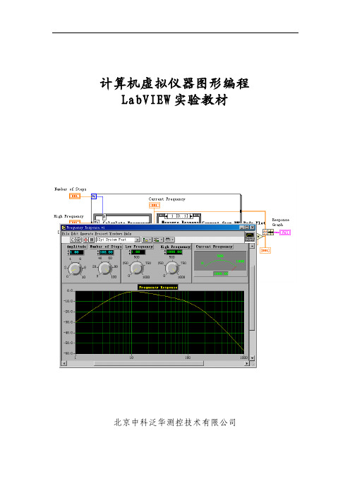
计算机虚拟仪器图形编程LabVIEW实验教材北京中科泛华测控技术有限公司目录第一课LABVIE W概述 (4)第一节虚拟仪器(VI)的概念 (4)第二节L AB VIEW的操作模板 (6)工具模板(Tools Palette) (6)控制模板(Controls Palette) (7)功能模板(Functions Palette) (8)第三节创建一个VI程序 (10)1. 前面板 (10)框图程序 (11)从框图程序窗口创建前面板对象 (12)4. 数据流编程 (12)第四节程序调试技术 (13)1. 找出语法错误 (13)2. 设置执行程序高亮 (13)3. 断点与单步执行 (13)4. 探针 (14)第五节练习1-1 (14)第六节把一个VI程序作为子VI程序调用 (17)第七节练习1-2 (18)第八节练习1-3 (20)第九节练习1-4 (22)第十节练习1-5 (24)第二课数据采集 (27)第一节概述 (27)第二节数据采集VI程序的调用方法 (29)第三节模拟输入与输出 (30)练习2-1 (31)第四节波形的采集与产生 (34)练习2-2 (35)第五节扫描多个模拟输入通道 (36)练习2-3 (36)第六节连续数据采集 (37)练习2-4 (38)第三课仪器控制 (40)第一节概述 (40)第二节串行通讯 (40)第三节IEEE488(GPIB)概述 (41)练习3-1 (43)第四节VISA编程 (44)练习3-2 (46)第五节用L AB VIEW编写仪器驱动程序 (47)第六节验证仪器驱动软件 (48)练习3-3 (49)第四课分析软件 (52)第一节概述 (52)第二节、高级分析功能程序 (52)第三节信号产生 (53)练习4-1 (53)第四节信号处理 (55)练习4-2 (55)第五节数字滤波器 (56)练习4-3 (57)第六节曲线拟合 (58)练习4-4 (59)练习4-5 (60)第五课实用工具软件包 (63)第一节概述 (63)第二节常用软件工具箱 (63)第三节分析工具软件 (65)第一课LabVIEW概述第一节虚拟仪器(VI)的概念使用LabVIEW开发平台编制的程序称为虚拟仪器程序,简称为VI。
北风网MFC实战系列第一讲VS2008 IDE环境的使用

标题栏
主按钮
导航标签 帮助按钮
新型菜单栏
快捷标题栏
视图工具面板
状态栏
文档视图
都从CWnd派生而来
扩展客户框架窗口
类OutlookBar控 件面板
扩展主框架窗口
MSDN = Microsoft Developer Network 是微软公司面向软件开发者的一种信息服务
技术文档 微软产品下载 MSDN WebCast 在线电子教程 Blog MSDN 杂志 网络虚拟实验室 BBS
应用程序
ODBC
ODBC驱动 ODBC驱动 ODBC驱动
Access
SQL Server
Oracle
WinSock是巴克利套接字标准在Windows系统中的实 现。 套接字本质是一组与具体网络协议无关的网络编程 接口。 Socket可以调用多种协议(TCP/IP V4/V6 、 AppleTalk、IPX、IrDA等)。 WinSock包含了巴克利 Socket风格的标准函数;还包 含一组Windows扩展函数,使程序员能利用Windows 消息机制进行编程。 MFC中包含的是WinSock1.1库的封装(CSocket、 CAsyncSocket)。 目前Windows平台上较新的WinSock版本是2.2版。
某复合文档
Word数据 片段 Visio数据 片段
Excel数据 片段 其它数据 片段n
ODBC(Open Database Connectivity, 开放数据库互连)是微软公司开放服 务结构(WOSA,Windows Open Services Architecture)中有关数据库的 一个组成部分。 它建立了一组规范,并提供了一组 对数据库访问的标准API(应用程序 编程接口)。 这些API利用SQL来完成其大部分任 务。 ODBC本身也提供了对SQL语言的支 持,用户可以直接将SQL语句送给 ODBC。 MFC中有较完整的ODBC接口封装 类(CDatabase、CRecordset、 CRecordView )。
tutorial

in mm and pixels. If positioned over a found spot, the spot coordinates and I/!(I) will be given. If positioned over a predicted spot position the hkl indices will be shown.Holding down the "Shift" key while the "Zoom" icon in the image is selected will show the image within the small dotted square zoomed within the solid square.2. Overview of iMosflmStart the program by typing "imosflm". After a brief pause, the following window will appear:The basic operations listed down the left hand side (Images, Indexing, Strategy, Cell Refinement, Integration, History) can be selected by clicking on the appropriate icon, but those that are not appropriate will be greyed-out and cannot be selected.2.1 Drop Down menusClicking on "Session" will result in a drop-down menu that allows you to save the current session or reload a previously saved session (or read/save a site file (see §14.1) or add images):Clicking on "Settings" will allow you to see (and modify) Experiment settings, Processing options and Environment variables. These will be described later.The three small icons below "Session" allow you to start a new session, open a saved session or save the current session. Moving the mouse over these icons will result in display of a tooltip describing the action taken if the icon is clicked.3. Adding images to a sessionTo add images to a session, use the "Add images..." icon:Select the correct directory from the pop-up Add Images window (the default is the directory in which iMosflm was launched). All files with an appropriate extension (which can be selected) will be displayed. Double-clicking on any file will result in all images with the same template being added to the session. The template is the whole part of the filename prefix, except the number field which specifies the image number. An alternative is to single-click on one image filename and then click on Open.To open one or several images only, check the 'Selected images only' box and then use click followed by Shift+click to select a range of images or Control+click to select individual image files as required.Loaded images will be displayed in the Images window with the start & end phi values displayed (as read from the image header).All images with the same template belong to the same "Sector" of data.Multiple sectors can be read into the same session. Each sector can have a different crystal orientation.Note that a "Warning" has appeared. Click anywhere on the “1 Warning” text to get a brief description of the warning. In this case it is because the direct beam coordinates stored in the MAR image plate images are not 'trusted' by MOSFLM and the direct beam coordinates have been set to the physical centre of the image. Click on the green tick on the right hand side to dismiss this warning; click anywhere outside the warning box to collapse the box; double-click the warning text itself and more details, hints and notes may be available from MOSFLM.The direct beam coordinates (read from the image header or set by MOSFLM) and crystal to detector distance are displayed. These values can be edited if they are not correct.Advanced Usage1. The phi values of images can be edited in the Image window. First click on the Image line to highlight it then click with themouse over the phi values to make them editable allowing new values to be given. These new values are propagated for all following images in the same sector. Starting values for the three missetting angles (PHIX, PHIY, PHIZ) may also beentered following the image phi values.2. To delete a sector click on the sector name to select it (it turns blue) then use the right mouse button on the sector to bring upa "delete" button. Move the mouse over the delete button (it turns blue) and click to delete the sector and its images.Individual images can be deleted from the Images pane in the same way.3. If one sector is added and used for indexing, and then a second sector from the same crystal is added, the matrix for thesecond sector will not be defined. To define it, double-click on the matrix name for the first sector, save it to a file, double-click on the matrix name (Unknown) for the new sector and read the matrix file written for the first sector. Alternatively, it is possible to "drag and drop" the matrix from the first sector onto the second sector (drop onto the sector itself, not the Matrix for the second sector).4. Image DisplayWhen images are added to a session, the first image of the sector is displayed in a separate display window.The "Image" drop-down menu allows display of the previous or next image in the series.The "View" drop-down menu allows the image to be displayed in different sizes (related by scale factors of two), based on the image size and the resolution of the monitor.The "Settings" drop-down menu allows the colour of the predictions to be changed (see Indexing §5.2 for the default colours),The line below allows selection of different images, either using right and left arrow or selecting one from the drop-down list of all images in that sector. Alternatively the image number can be typed into the "Go to" entry box. The "Sum" entry box will allow the display of the sum of several images, but this is not yet fully implemented.The image being displayed can also be changed by double-clicking on an image name in the "Images" pane of the main window. This will also re-active the image window if it has been closed."+" and "-" will zoom the image without changing the centre. The "Fit image" icon will restore the image to its original size (right mouse button will have the same effect). The "Contrast" icon will give a histogram of pixel values. Use the mouse to drag the vertical dotted line, to the right to lighten the image, to the left to darken it. Try adjusting the contrast. The "Lattice" entry window can be used when processing images with multiple lattices present, see multiple lattices §5.3)4.1 Display IconsThe eight icons on the left, control the display of the direct beam position, spots found for indexing, bad spots, predicted spots, masked areas, spot-finding search area, resolution limits and display of the active mask for Rigaku detectors respectively.These are followed by icons for Zoom, Pan and Selection tools, and tools for adding spots manually (for indexing), editing masks, circle fitting and erasing spots or masks.Next on this toolbar are the entry boxes for h, k & l and a button to search for this hkl among the predicted spots displayed on the image. The button resembles a warning sign if the given hkl cannot be found, but a green tick if it is found. The final icon relates to processing images with multiple lattices, (see multiple lattices §5.3) and is not described here.4.1.1 Masked areas - circular backstop shadowSelect the masked area icon. A green circle will be displayed showing the default position and size of the backstop shadow.Make sure that the Zoom icon (magnifying glass) is selected and use the left-mouse-button (abbreviated to LMB in following text) to drag out a rectangle around the centre of the image. The inner dotted yellow rectangle will show the part of the image that will actually appear in the zoomed area.Choose the Selection Tool. When placed over the perimeter of the circle, the radius of the circular backstop shadow will be displayed. Use the LMB to drag the circle to increase its diameter to that of the actual shadow on the image. The position of the circle can be adjusted with LMB placed on the cross that appears in the centre of the green circle. Adjust the size and position of the circle so that it matches the shadow.4.1.2 Masked areas - general exclusionsChoose the Masking tool. Any existing masked areas will automatically be displayed. Use LMB to define the four corners of the region to be masked. When the fourth position is given, the masked region will be shaded. This region will be excluded from spot finding and integration. This provides a powerful way of dealing with backstop shadows. To edit an existing mask, choose the Selection tool and use the LMB to drag any of the four vertices to a new position.To delete a mask, choose the Spot and mask eraser tool. Place the mouse anywhere within the shaded masked area, and use LMB to delete the mask. Delete any masks that you have created.4.1.3 Spot search areaSelect the Show spotfinding search area icon. The inner and outer radii for the spot search will be displayed as shown below. If the images are very weak, the spot finding radius will automatically be reduced, but this provides additional control.Either can be changed by dragging with the LMB. Do not change the radii for these images.Advanced UsageThe red rectangle displays the area used to determine an initial estimate of the background of the image. It is important that this does not overlap significant shadows on the image. It can be shifted laterally or changed in orientation (in 90° steps) by dragging with the LMB.4.1.4 Resolution limitsSelect the Show resolution limits icon. The low and high resolution limits will be displayed. The resolution limits can be changed by dragging the perimeter of the circle with LMB (make sure that the Selection Tool has been chosen). The resolution limits will affect Strategy, Cell refinement and Integration, but not spot finding or indexing. The low resolution is not strictly correct (it falls within the backstop shadow) but does not need to be changed because spots within the backstop shadow will be rejected.4.1.5 Zooming and PanningFirst select a region of the image to be zoomed with the Zoom tool.Select the Pan tool and pan the displayed area by holding down LMB and moving the mouse. This is very rapid on a local machine, but may be slow if run on a remote machine over a network.4.1.6 Circle fittingThe circle fitting tool can be used to determine the direct beam position by fitting a circle to a set of points on a powder diffraction ring on the image (typically due to icing) or to fit a circular backstop shadow (although using the masking tool is probably easier).Select the circle fitting tool. Three new icons will appear in the image display area. There are two (faint) ice rings visible on the image at 3.91Å and 3.67Å. Click with LMB on several positions (6-8) on the outer ring (as it is slightly stronger). Then click on the top circular icon.A circle that best fits the selected points (displayed as yellow crosses) will be drawn, and the direct beam position at the centre of this circle will be indicated with a green cross. The direct beam coordinates will be updated to reflect this new position.5. Spot finding, indexing and mosaicity estimationWhen images have been added, the "Indexing" operation becomes accessible (it is no longer greyed-out).Click on Indexing. This will bring up the major Indexing window in place of the Images window.5.1 Spot FindingBy default, two images 90 degrees apart in phi (or as close to 90 as possible) will be selected and a spot search carried out on bothimages (This is controlled by the "Automatically find spots on entering Autoindexing" button in the Spot finding tab of Processing options).Found spots will be displayed as crosses in the Image Display window (red for those above the intensity threshold, yellow for those below). The intensity threshold normally defaults to 20, but will be automatically reduced to 10 or 5 for weak images. The threshold is determined by the last image to be processed.The number of spots found, together with any manual additions or deletions, are also given.Images to be searched for spots can be specified in several ways:1. Simply type in the numbers of the images (e.g. 1, 84 above).2. Use the "Pick first image" icon (single blue circle).3. Use the "Pick two images ~90 apart" icon (two blue circles) . This is the default behaviour.4. Use the "Select images ..." icon (multiple circles). If selected, all images in the sector are displayed in a drop-down list. Clickon a image to select it, then double-click on the search icon (resembling a target) for that image to run the spot search. The image will move to the top of the list (together with other images that have been searched).Images to be used for indexing can be selected from those that have been searched by clicking on the "Use" button. If this box was previously checked, then clicking will remove this image from those to be used for indexing. It can be added again by clicking the "Select images ..." icon and clicking on the "Use" box.5.1.1 Difficult imagesParameters affecting the spot search can be modified by selecting the "Settings" drop-down window and selecting "Processing options". The resulting new window contains six tabs relating to Spot finding, Indexing, Processing, Advanced refinement, Advanced integration and Sort, Scale and Merge.The Spot finding window allows the Search area, Spot discrimination parameters, Spot size parameters, Minimum spot separation and Maximum peak separation within spots (to deal with split spots) to be reset. It also allows the choice between a local background determination (preferred) and a radial background determination. The local background method also uses an improved procedure for recognising closely spaced spots. The only parameters commonly changed are:1. Minimum spot separation. This should be the size (in mm) of an average spot (not a very strong spot). Change to valuesestimated by manual inspection of spots if there are difficulties due to badly split spots. This separation parameter is very important when spots are very close, but usually the program will determine a suitable value.2. Minimum pixels per spot. Default value 6, but this will be reduced automatically if spots are very small (eg in situ screeningand microfocus beam).3. Local background box size. Reducing this from 50 to (say) 20 can reduce the number of "false" spots found near any sharpshadow on the image.For data collected in-house spots can be quite large and rather weak. In such cases the spot finding parameters are automatically changed, but some improvement may still be obtained by the following:1. Reduce the spot finding threshold (default 3.5), e.g. to2.2. Increase the minimum number of pixels per spot (default 30) to 20 or 40.3. Set the minimum spot separation to a sensible value, e.g. 1.5mm5.2 IndexingProviding there are no errors during spot finding, indexing will be carried out automatically after spot finding (This is controlled by the "Automatically index after spot finding" button in the Indexing tab of Processing options). If the image selection or indexing parameters are changed, the "Index" button must be used to carry out the indexing.Autoindexing will be carried out by MOSFLM using spots (above the threshold) from the selected images. The threshold is set by MOSFLM but can be changed using the entry box in the toolbar. The list of solutions, sorted by increasing penalty score, will appear in the lower part of the window. The preferred solution will be highlighted in blue. There will usually be a set of solutions with low penalties (0-20) followed by other solutions with significantly higher penalties. The preferred solution is that with the highest symmetry from the group with low penalty values.Note that all these solutions are really the same P1 solution transformed to the 44 characteristic lattices, with latticesymmetry constraints applied. Therefore, if the P1 solution is wrong, then all the others are wrong as well.For solutions with a penalty less than 50, the refined cell parameters ("ref") will be shown. This can be expanded (click on the + sign) to show the "reg" unrefined but regularised cell (symmetry constraints applied) and the "raw" cell (no symmetry constraints applied).The rms deviation (rmsd) or error in predicted spots positions (!(x,y) in mm) and the rms error in (!(") in degrees) are given for each solution.Usually the penalty will be less than 20 for the correct solution, although it could be higher if there is an error in the direct beam coordinates (or distance/wavelength). The rmsd (error in spot positions) will typically be 0.1-0.2mm for a correct solution, but if the spots are split or very elongated it can be as high as 1mm or higher.The predicted spot positions for the highlighted solution will be shown on the image display with the following default colour codes:Blue:Fully recorded reflectionYellow:Partially recorded reflectionRed:Spatially overlapped reflection... these will NOT be integratedGreen:Reflection width too large (more than 5 degrees)... not integrated.These colours may be adjusted via the "Settings - Prediction colour" item in the Image display window.Providing there are no errors in the indexing, MOSFLM will automatically estimate the mosaic spread (mosaicity) based on the preferred solution.Select other solutions with a higher penalty and see how well the predicted patterns match the diffraction image.The rmsd and visual inspection of the predicted pattern are the best ways of checking if a solution is correct. If the agreement is not good, then the autoindexing has probably failed.5.2.1 If the indexing fails - Direct beam searchThe indexing is very sensitive to errors in the direct beam coordinates. For a correct indexing solution, these should be correct to better than half the minimum spot separation. Check, for example, that the current direct beam position is behind the backstop. If there are any ice rings, these can be used to determine the direct beam position (see Circle fitting §4.1.6 ).If the accuracy of the direct beam coordinates (generally read from the image header) is uncertain, the program can perform a grid search around the input coordinates. The number and the size of the steps can be set from the Indexing tab of the Processing options menu (see Settings - Processing options §2.1) but defaults to two steps of 0.5mm on each side of the input coordinates. The direct beam search is started by clicking on the text "Search beam-centre" in the Indexing pane. While in progress, it can be stopped by clicking on the same place, the text of which is now "Abort beam-centre".The indexing will be carried out for each set of starting coordinates (Beam x and Beam y in the table which appears) and, if a solution is found, the refined beam coordinates (Beam x ref, Beam y ref), the unit cell parameters of the triclinic solution and the rmsd error in spot coordinates and in phi will be listed. The correct solution will generally be the one with the smallest rms error in spot positions (!(x,y)). To make it simpler to identify the correct solution, once the grid search has finished the solutions will be sorted on !(x,y), so the correct solution will be at the top of the list. When sorting the solutions, those which have smaller cell parameters will be listed first, as it is possible to have a small!(x,y) value for an incorrect solution with a much larger unit cell.Note that only the triclinic (P1) solution will be listed. To complete the indexing, double-click on the chosen solution, and the full indexing will carried out for these beam coordinates, with the solutions appearing in the upper window. The results of the direct beam search can be hidden (collapsed) by clicking on the [-] symbol next to "Search beam-centre" and recovered by clicking on [+]5.2.2 If the indexing fails - Other parameters.Errors in other physical parameters (wavelength, crystal to detector distance) can also result in failure. All these parameters should be checked.Several parameters used in autoindexing can also be adjusted using entry fields and buttons that appear in the Indexing toolbar.Weak images1. MOSFLM automatically reduces the I/!(I) threshold for weak images and it may also reduce the resolution to 4# but lowervalues can be tried. It is important not to include spots that are not "real" - a small number of false spots can prevent theindexing from working.2. Try changing parameters for spot finding (see Difficult images §5.1.1)Multiple lattices1. Try increasing the I/!(I) threshold (default 20), for example to 40 or 60, so that only spots from the stronger lattice are selected.This can be done by entering a new value in the leftmost of the circled icons above (and also via the using the Indexing tab of Processing options).All cases1. Include more images in the indexing.2. Select images that show the clearest lunes and/or have the best spot shape.3. In case the crystal orientation has changed, or if you are unsure of the direction of positive rotation in phi, try indexing usingonly one image.4. If the cell parameters are known, reduce the maximum allowed cell edge to the known maximum cell edge. This can sometimeshelp filter incorrect solutions, but use with caution as often this needs to be ~twice the largest cell for successful indexing.5. If the detector distance is uncertain, and the images are high resolution (e.g. 2#), allow the detector distance to refine duringcell refinement. Use with caution.5.3 Indexing multiple lattices simultaneouslyThis is a new feature and is still undergoing development. It is most likely to succeed when the different lattices are clearly separated, at least at higher resolution. If the images shows badly split spots with several components (each arising from a sub-crystal with a slightly different orientation) then indexing may well still be impossible.After spot finding, examine the image to ensure that spots that are close to each other but belong to different lattices have been identified as separate spots, and not treated as a single split spot (in which case the red cross will lie midway between the two spots). Adjusting the minimum spot separation (Settings -> Processing options -> Spot finding) can help in resolving close spots. It may also help to increase the inner radius of the spot search region (see Spot search area §4.1.3) so that low resolution reflections where the spots are not really separated are excluded from the search.The following procedure usually provides the best chance of success:1. Select appropriate images for use in indexing. The separation of the lattices can be clearer on some images than others. Ideally choose several images widely separated in phi.2. Do a normal (single lattice) indexing first. This will usually work, but will give a high positional rmsd because of the presence of more than one lattice. This step is important because it will result in more accurate direct beam coordinates, which are crucial for multi-lattice indexing.3. Select “Index multiple lattices” from the drop-down option next to the “Index” button.The indexing results for different lattices will be presented in different tabs, while the selected solution for each lattice will be shown in the lower "Summary" window. Currently a maximum of 5 lattices can be handled. The figure below shows a case where 3 different lattices were found.4. Judge the success of indexing by examining the lattice type and the cell parameters obtained for the different lattices (the cells should be very similar) and checking that the predictions match the observed spots. The rmsd values for correct lattices should also be significantly smaller than the value obtained in the initial (single lattice) indexing. It may be necessary to manually select a different autoindexing solution for some lattices in order to get consistent results for the different lattices.The "Split" column in the lower pane indicates the angle between the reference lattice (with value "-") and the other lattices. This is only calculated when the lattices have the same lattice type. In this case, the angles between lattice 1 and lattices 2 & 3 are 3.4 and 1.6 degrees.If a lattice is clearly incorrect, it can be deleted by highlighting that lattice (in the lower pane that summarises the results) and using the right mouse button to select “delete”.The predictions for different lattices can be displayed either by highlighting the lattice in the Summary window or by using the lattice selector in the image display pane.In the image display, spots in different lattices that overlap with each other are shown in magenta. Only the summed intensity will be measured for these reflections.The predictions for all lattices can be shown by selecting the “merge lattices” icon in the image display.This can be useful to check if all the lattices have been successfully indexed, because all spots in the image should then be predicted. In the display, predictions from lattice 1,2,3,4,5 are shown in blue, yellow, red, green and magenta with no distinction made between fully and partially recorded reflections or spatial overlaps.5.3.1 Practical TipsBeware of solutions where the lattices only vary in orientation by a small angle (less than 1 degree) as these are often different solutions for the same lattice. The difference in orientation between lattices is given by the “split” column in the Summary window, but this is only calculated if the lattices have the same lattice type. Differences are all relative to one lattice, which will display a split angle as “-“. To calculate the angles relative to a different lattice, open the tab for that lattice, select a different solution to that currently selected and then select the original solution – this will trigger recalculation of the split angles relative to that lattice. Other parameters that can influence the indexing are the ”Maximum deviation from integral hkl” (default 0.2 when indexing multiple lattices, otherwise 0.3) and “Number of vectors to find for indexing” (default 30). These can be changed via the Indexing tab of the “Processing Options” that can be selected from the “Settings” menu item. Values between 0.15 and 0.25 might be helpful for the first parameter and increasing the number of vectors from 30 to 50 can also help. At present there is no defined protocol for changing the default parameter values for particular cases, it has to be done by trial and error.Experience so far has shown that selecting appropriate images and adjusting the maximum cell length used in indexing have the biggest effect. The optimum value for the maximum cell length will normally lie between one and three times the largest cell dimension, but it is worth varying this in steps of between 25 and 50 Å, as the indexing can be very sensitive to this parameter.For a more complete discussion of multiple lattice indexing see: Powell, H.R., Johnson, O. & Leslie, A.G.W. 2013. Autoindexing diffraction images with iMosflm. Acta Cryst. D69, 1195-1203.5.4 Space group selectionNote that the indexing is based solely on information about the unit cell parameters. It will therefore be very difficult (or impossible) to determine the correct Laue group in the presence of pseudosymmetry. For example, a monoclinic space group with $ ~ 90 will appear to be orthorhombic; an orthorhombic space group with very similar a and b cell parameters will appear to be tetragonal. These can only be distinguished when intensities are available (i.e. after integration) by running POINTLESS.In addition, it is not possible to distinguish between Laue Groups 4/m and 4/mmm, 3 and 3/m, 6/m and 6/mmm, m3 and m3m. This will not affect integration of the images, but it will affect the strategy calculation. In the absence of additional information, the lower symmetry should be chosen for the strategy calculation to ensure that a complete dataset is collected.The presence of screw axes also cannot be detected, so there is no basis on which to distinguish P21 from P2 etc. This does not affect。
VT教程:水晶石教育_初级程序_VT基础 via 叮当

•
•
Virtools
初级程序第1周
一个软件开发包 (SDK)
Virtools作为一个软件开发包,提供了可 以访问行为引擎和渲染引擎的接口.通过SDK, 你可以:
• • • • • • 创建或修改现有的BB 创建新的参数类型 创建新的文件格式读取插件 替换掉virtools的渲染引擎,使用自己订制的渲染引擎 可以自己定制可执行文件(.exe) 可以充分扩展渲染引擎部分,使渲染功能更完善
1、显示全部 2、隐藏全部 3、 隐藏选取 4、 隐藏其它
Virtools
初级程序第1周
1
1、展开
2
3
4
1、重置缩放位置 2、画面缩放 3、除错器 4、轨迹器 5、连结错误器 6、无效模组
2、关闭 3、选取器 4、讯息发送器 5、查找
1Leabharlann 2345
1、显示/ 隐藏区域参数 2、 显示/ 隐藏角本项目 3、 显示/ 隐藏控制节点 4、 显示/ 隐藏延迟值 5、模组连结属性设定 6、 显示/ 隐藏优先属性
Virtools
初级程序第1周
一、软件操作介绍
1.1软件界面
1 菜单栏
Virtools
初级程序第1周
2 三维编 辑区
3 行为模 块和素 材库
4 角本流程 图和层级 管理器 5 状态栏
1.1软件界面
Virtools
1、菜单栏(Menu Bar):
主菜单是个典型的功能表单,包括档案、资源、编辑、控制选 单、帮助
1
2
1、显示/关闭3D网格,每格代表1米 2、显示/关闭2D网格
1、建立相机 2、建立灯光 3、建立3D物体 4、建立曲线 5、建立遮罩
1
LW2008SystemTapTutorial

•Student:
−How can I learn more about the inner workings of a kernel subsystem?
12
Get it on Fedora
•Do it all with yum:
yum install systemtap yum install kernel-devel gcc make
•String type 'string'
−Zero-terminated string in a fixed-length buffer −Supports concatenation and comparison: . .= < > <= >= == !=
•Associative arrays (global only)
•Kernel Developer:
−How can I add debug statements easily without going through the insert/build/reboot cycle?
•Application Developer:
−How can I improve the performance of my application in Linux?
# stap -e 'probe begin { println("Hello world!") }' (1---)(2)(3----------)(4-------------------------)
1. 'stap' is the main executable for SystemTap
CMG软件Tutorial STARS Revised_Sept2008_CCC(中文)
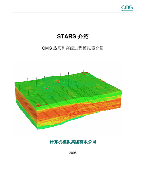
STARS介绍CMG热采和高级过程模拟器介绍计算机模拟集团有限公司2008目录图的列表 (2)图的列表 (2)创建一个蒸汽模型 (2)打开BUILDER (2)利用“Quick Pattern”来创建一个STARS稠油数据库 (2)通过黑油PVT关系生成STARS流体模型属性 (4)创建相对渗透率数据 (7)随温度变化的相对渗透率 (8)为蒸汽注入修改相对渗透率曲线(组分关系式) (12)创建初始条件 (16)创建数值控制 (16)完成井的射孔 (16)添加组Adding Groups (17)添加操作约束 (17)添加日期 (18)输出基本性质和井的信息 (18)利用Builder验证数据库 (19)运行模拟器 (19)在STARS中建立一个循环蒸汽模拟模型 (23)注水 (30)一次采油量 (31)图的列表图1:General Property Specification 电子表格 (3)图 2:热采岩石类型 (3)图3:下拉框 (17)图4:限制和注入流体 (18)图10: I/O Control (19)图5:Log File Summary (20)创建一个蒸汽模型打开BUILDER1. 通过双击相应的图标打开Builder。
2. 选择:•STARS模拟器,SI单位制,Single Porosity(单孔)•开始日期为2005-01-013. 点击两次OK。
利用“Quick Pattern”来创建一个STARS稠油数据库4. 点击Reservoir (在工具条中或在树状视图中) 并且Create Grid.5. 选择Quick Pattern Grid 输入如下所示的一些信息:注:单位是自动应用的井网类型:Normal 5-spot 油藏的顶深:500 (m)井区的面积:10 (acres) 大概的网格块厚度: 4 (m)油藏的厚度: 30 (m) 大概的X,Y方向上网格块尺寸:6 (m)6. 点击Calculate。
Tutorial 使用指南
使用指南(Tutorial)修订版序从首次接触这个软件到现在,有一段时间了。
那时由于急着使用,因此对一些认为不太重要的地方没有进行整理。
后来才发现,其实每一部分都是很有用的。
此修订,一个是将LineSim(Tutorial)与后加的Crosstalk(Tutorial)的目录统一起来,再有就是原文基础上增加了多板仿真(Tutorial)一节。
同样,对于那一时期我整理的BoardSim 、LineSim使用手册,也有同样的一个没有对一些章节进行翻译整理问题(当初认为不太重要)。
而实际上使用时,有一些东西是非常重要的,同时也顺便进行了翻译。
此外,通过使用,对该软件有了更多一些理解,显然以前只从字面翻译的东西不太好理解,等我有时间将它们重新整理后,再提供给初学的朋友。
对在学习中给予我大量无私帮助的Aming、pandajohn、lzd 等网友表示忠心的感谢。
P o q i0552002-8-202002-8-20目录使用指南(TUTORIAL ) 1 第一章 LINESIM4 1.1 在L INE S IM 里时钟信号仿真的教学演示 4 第二章 时钟网络的EMC 分析 7 2.1 对是中网络进行EMC 分析7 第三章 LINESIM'S 的干扰、差分信号以及强制约束特性 8 3.1 “受害者”和 “入侵者” 8 3.2如何定线间耦合。
8 3.3 运行仿真观察交出干扰现象9 3.4 增加线间距离减少交叉干扰(从8 MILS 到 12 MILS ) 93.5 减少绝缘层介电常数减少交叉干扰 93.6 使用差分线的例子(关于差分阻抗) 93.7仿真差分线 10第四章 BOARDSIM114.1 快速分析整板的信号完整性和EMC 问题 11 4.2 检查报告文件 11 4.3 对于时钟网络详细的仿真 11 4.4 运行详细仿真步骤: 11 4.5 时钟网络CLK 的完整性仿真 12 第五章 关于集成电路的MODELS 145.1 模型M ODELS 以及如何利用T ERMINATOR W IZARD 自动创建终接负载的方法 14 5.2 修改U3的模型设置(在EASY.MOD 库里CMOS,5V,FAST ) 14 5.3 选择模型(管脚道管脚)C HOOSING M ODELS I NTERACTIVELY (交互), P IN -BY -P IN 14 5.4 搜寻模型(F INDING M ODELS (THE "M ODEL F INDER "S PREADSHEET ) 15 5.5 例子:一个没有终接的网络 15 第六章 BOARDSIM 的干扰仿真 186.1 B OARD S IM 干扰仿真如何工作 186.3仿真的例子:在一个时钟网络上预测干扰 18 6.3.1加载本例的例题“DEMO2.HYP” 18 6.3.2A UTOMATICALLY F INDING "A GGRESSOR"N ETS 18 6.3.3为仿真设置IC模型 19 6.3.4查看在耦合区域里干扰实在什么地方产生的 19 6.3.5驱动IC压摆率影响干扰和攻击网络 20 6.3.6电气门限对比几何门限 20 6.3.7用交互式仿真"CLK2"网络 20 6.4快速仿真:对整个PCB板作出干扰强度报告 20 6.5运行详细的批模式干扰仿真 21第七章关于多板仿真237.1多板仿真例题,检查交叉在两块板子上网络的信号质量 23 7.2浏览在多板向导中查看建立多板项目的方法 24 7.3仿真一个网络A024 7.4用EBD模型仿真24HyperLynxHyperLynx是高速仿真工具,包括信号完整性(signal-integrity)、交叉干扰(crosstalk)、电磁屏蔽仿真(EMC)。
实验三 Tutorial 3 vi 基本操作
Tutorial 3 vi 基本操作1 实验简介Linux 本质上是一个文本驱动(text-driven)的操作系统。
vi是最基本的文本编辑工具,它是一个全屏幕文本编辑器,具有文本编辑所需的所有功能。
掌握vi的命令和使用方式,对于学习Linux 操作系统的人员来说是非常重要的。
本次实验内容包括:vi三种模式之间的切换、vi基本指令的使用。
2 实验目的(1)学会使用vi编辑器,掌握vi编辑器的一些常用指令。
(2)掌握vi各类命令的使用方法。
3 实验准备(1)熟练掌握vi三种工作模式的转换。
(2)熟练掌握vi的基本命令。
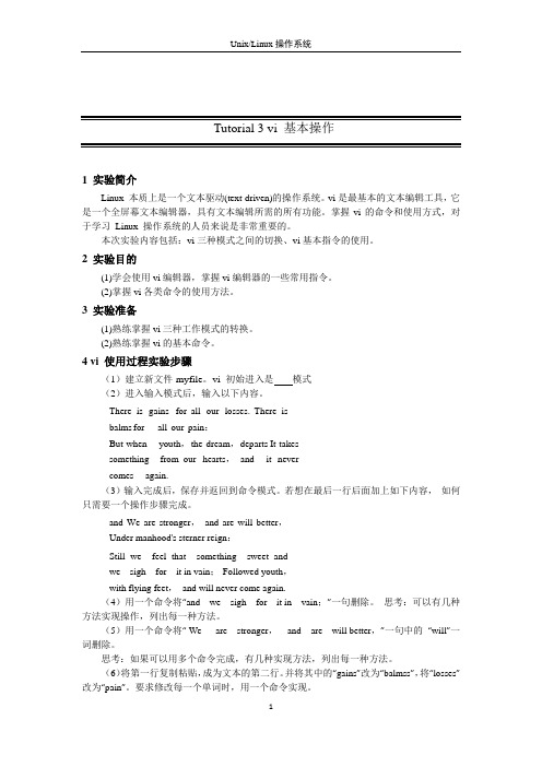
4 vi 使用过程实验步骤(1)建立新文件myfile。
vi 初始进入是模式(2)进入输入模式后,输入以下内容。
There is gains for all our losses. There isbalms for all our pain:But when youth,the dream,departs It takessomething from our hearts,and it nevercomes again.(3)输入完成后,保存并返回到命令模式。
若想在最后一行后面加上如下内容,如何只需要一个操作步骤完成。
and We are stronger,and are will better,Under manhood's sterner reign:Still we feel that something sweet andwe sigh for it in vain;Followed youth,with flying feet,and will never come again.(4)用一个命令将“and we sigh for it in vain;”一句删除。
思考:可以有几种方法实现操作,列出每一种方法。
(5)用一个命令将“ We are stronger,and are will better,”一句中的“will”一词删除。
tutorial节选

Things to Know Before Getting Started with eQUEST Whole building analysis. eQUEST is designed to provide whole Building performance analysis to buildings professionals, i.e., owners, designers, operators, utility & regulatory personnel, and educators. Whole building analysis recognizes that a building is a system of systems and that energy responsive design is a creative process of integrating the performance of interacting systems, e.g., envelope, fenestration, lighting, HVAC, and DHW.在开始之前需要知道的事情与eQUEST关于整个建筑的分析。
eQUEST旨在提供整个建筑性能分析建筑专业人士,即所有者,设计师、运营商、实用工具和监管人员,和教育家。
从整个建筑分析认识到建筑是一个系统的系统和能量响应设计是一种创造性的整合过程性能交互的系统,例如,维护结构、开窗、照明、空调和DHW。
Therefore, any analysis of the performance consequences of these building systems must consider the inter actions between them … in a manner that is both compre hensive and affordable (i.e., model preparation time, simulation runtime, results trouble shooting time, and results reporting).因此,任何分析的性能影响这些建筑系统必须考虑…它们之间的交互的方式,既全面和负担得起的(例如,模型的准备时间,模拟运行时间,结果故障排除时间,和结果报告)。
VI编辑器详解
鸟哥的 Linux 私房菜VI 编辑器高级详细教程整理自台湾鸟哥的LINUX私房菜网站Qq交流群:101391297系统管理员的重要工作就是得要修改与设定某些重要软件的设定文件,因此至少得要学会一种以上的文字接口的文书编辑器。
在所有的 Linux distributions 上头都会有的一套文书编辑器就是 vi ,而且很多软件预设也是使用 vi 做为他们编辑的接口, 因此鸟哥建议您务必要学会使用 vi 这个正规的文书编辑器。
此外,vim 是进阶版的 vi , vim 不但可以用不同颜色显示文字内容,还能够进行诸如 shell script, C program 等程序编辑功能, 你可以将 vim 视为一种程序编辑器!鸟哥也是用 vim 编辑鸟站的网页文章呢! ^_^1. vi 与 vim1.1 为何要学 vim2. vi 的使用2.1 简易执 行范例2.2 按键说明2.3 一 个案例的练习2.4 vim 的暂存档、救援回复与开启时的警告讯息3. vim 的额外功能3.1 区块选 择(Visual Block)3.2 多 档案编辑3.3 多视 窗功能3.4 vim 环境设定与记录: ~/.vimrc, ~/.viminfo3.5 vim 常用指令示意图4. 其它 vim 使用注意事项4.1 中 文编码的问题4.2 DOS 与 Linux 的断行字符: dos2unix, unix2dos4.3 语系编码 转换: iconv5. 重点回顾6. 本章习题7. 参考资 料与延伸阅读8. 针对本文的建议:/viewtopic.php?t=23883vi 与 vim由前面一路走来,我们一直建议使用文字模式来处理 Linux 的系统设定问题,因为不但可以让你比较容易了解到 Linux 的运作状况,也比较容易了解整个设定的基本精神,更能『保证』你的修改可以顺利的被运作。
所以,在 Linux 的系统中使用文字编辑器来编辑你的 Linux 参数设定档,可是一件很重要的事情呦!也因此呢,系统管理员至少应该要熟悉一种文书处理器的!Tips:这里要再次的强调,不同的 Linux distribution 各有其不同的附加软件,例如 RedHat Enterprise Linux 与 Fedora 的 ntsysv 与 setup 等,而 SuSE 则有 YAST 管理工具等等, 因此,如果你只会使用此种类型的软件来控制你的 Linux 系统时,当接管不同的 Linux distributions 时,呵呵!那可就苦恼了!在 Linux 的世界中,绝大部分的设定档都是以 ASCII 的纯文字形态存在,因此利用简单的文字编辑软件就能够修改设定了! 与微软的 Windows 系统不同的是,如果你用惯了 Microsoft Word 或 Corel Wordperfect 的话,那么除了 X window 里面的图形接口编辑程序(如 xemacs )用起来尚可应付外,在 Linux 的文字模式下,会觉得文书编辑程序都没有窗口接口来的直观与方便。
Vi Vim编辑器工具软件使用手册
在多个文件之间的编辑切换:
在末行模式下:
:n 载入下一个文件 :N 载入上一个文件
当完成一个文件的编辑后,需要保存该文件,才可切换
两个文件之间的编辑切换:
命令模式下:
ctrl+shift+6
末行模式下:
:e#
vi命令大全
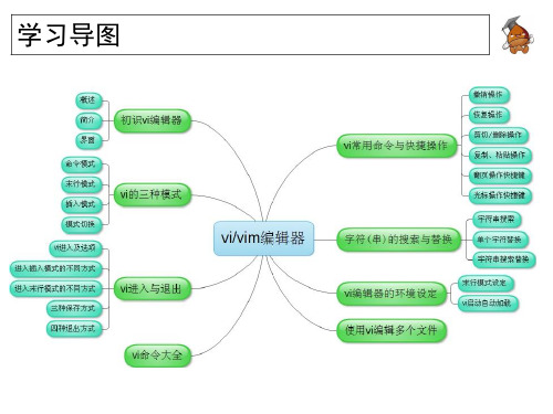
总结整理
vi打开、退出与保存退出 vi进入插入,末行模式的方法 vi返回命令模式的方法 vi的剪切/删除、复制、粘贴方法 vi的翻页、光标操作方法 vi的搜索与替换方法 vi编辑多个文件的方法 vi的环境设定以及自动启动配置文件
2、利用vi打开vi_test文件,打开时自动定位在第二行。
在第二行结尾,输入123456,回到命令模式。 在第二行开头,输入567890,回到命令模式。 另存为文件为vi_test1。
3、利用vi打开vi_test1
在第一行开头,输入abcdef,回到命令模式。 放弃保存,并退出。
Vi常用命令与快捷操作
:
命令
查找(自顶向下)
?
查找(自底向上)
三种保存方式
有三种方法保存当前编辑的文件 在末行模式下:
:w [filepath] 保存当前编辑的文件 :w! [filepath] 强制保存文件,若文件已存在则强行覆盖 若[filepath] 有指定,表示另存为文件。
四种退出方式
有四种方法可以退出vi返回到shell命令提示符:
实验与练习
vi的进与退出练习
1、通过vi打开/etc/passwd文件,并定位到第10行,然后退出。 2、使用vi新建文件,退出时保存路径名为/root/vi_test。 3、使用vi打开之前创建的/root/vi_test文件,在命令模式按键盘i 键进入插入模式,输入“hello world”,保存并退出。
Verilog_tutorial 文档
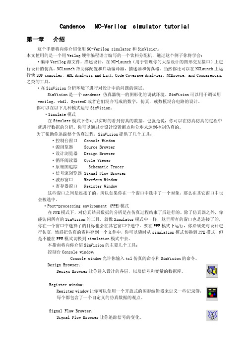
Candence NC-Verilog simulator tutorial第一章介绍这个手册将向你介绍使用NC-Verilog simulator和SimVision。
本文使用的是一个用Veilog硬件编程语言编写的一个饮料分配机,通过这个例子你将学会:·编译Verilog源文件,描述设计,在NC-Launch(用于管理你的大型设计的图形交互接口)上进行设计的仿真。
NCLaunch帮助你配置和启动编译器,描述器和仿真器。
当然你还可以在NCLaunch上运行像SDF compiler,HDL Analysis and Lint,Code Coverage Analyzer,NCBrowse,and Comparescan.之类的工具。
·在SimVision分析环境下进行对设计中的问题的调试。
SimVision是一个candence仿真器统一的图形化的调试环境。
SimVision可以用于调试用verilog,vhdl,SystemC或者它们混合写成的数字,仿真,或数模混合电路的设计。
你可以在以下几种模式运行SimVision:·Simulate模式在Simulate模式下你可以实时的看到仿真的数据。
也就是说,你可以在仿真仿真的过程中就进行数据的分析。
你可以通过对设计设置断点和分步来达到控制仿真的。
为了帮助你追踪整个仿真过程,SimVision提供了几个工具:·控制台窗口Console Window·源浏览器Source Browser·设计浏览器Design Browser·循环阅读器Cycle Viewer·原理图追踪Schematic Tracer·信号流浏览器Signal Flow Browser·波形窗口Waveform Window·寄存器窗口Register Window这些窗口之间是连接了的,所以如果你在一个窗口中选中了一个对象,那么在其它窗口中也会被选中。
vim tutorial
Vim Hands-On Tutorial Computer Science DepartmentINTRODUCTION: (3)T UTORIAL R EQUIREMENTS: (3)T UTORIAL C ONVENTIONS: (3)A BOUT V IM (3)EDITING BASICS: (4)I NVOKING V IM (4)V IM M ODES:C OMMAND AND I NSERT (4)O PENING E XISTING F ILES AND S AVING (OR N OT) (5)M OVING A ROUND (8)O OPS!(U NDOING M ISTAKES) (8)TEXT SEARCHING: (10)S EARCH BY P ATTERN (10)S EARCHING BY L INE N UMBER (12)S UBSTITUTION: (13)MANIPULATING TEXT: (14)C OPYING (14)D ELETING/C UTTING (14)P ASTING (14)RECOVERING FROM A SYSTEM CRASH: (15)CUSTOMIZING VIM: (15)REFERENCES (16)EVALUATION (17)Introduction:Tutorial Requirements:•Computer Science Department Linux account•Familiarity with standard feature and functions of a text editor•Previous experience working in the Linux environment, attended a session of the CS Department Hands-on Linux Tutorial, or completed at least one CS course that required the use of the Linux environment.Tutorial Conventions:•Vim Commands are in italics.•Tutorial Examples Commands are in bold.•Keyboard strokes are in angle brackets, i.e. <enter> to strike the enter keyAbout VimVim is a text editor that stands for “Vi Improved”. As the name suggests, it is upwards compatible to Vi and it can be used to edit all kinds of plain text documents. It's typically used to edit program source files and Linux/Unix system configuration files. It also happens to be installed by default on almost every Unix or Unix-clone (i.e. Linux) platform.[1]Some improvements that Vim has over Vi are multi-level undo, multi windows and buffers, syntax highlighting, command line editing, filename completion, online help, visual selection, etc.. See :help vi_diff.txt for a summary of the differences between Vim and Vi. [1]While running Vim, help can be obtained from the on-line help system, with the :help command.Most often Vim is started to edit a single file with the command:vim filenameMore generally, Vim is started with:vim [options][filelist]A list of options can be obtained by reading the manual pages on Vim using the command:man vimThere is an interactive Vim tutorial program that you can work through by using the command:vimtutorEditing Basics:Invoking Vimvim <Enter>You will see the welcome screen in the Vim programappear:Vim Modes: Command and InsertThere are two primary modes in Vim: Command and Insert. Vim starts in Command mode. You cannot insert text while in Command mode.type:iThe word ‘insert’ should appear at the bottom of thescreen indicating you are in Insert mode.Now you can insert text at the cursor position.Type the following traditional Hello World programinto the buffer:#include<iostream>std;usingnamespaceintmain(){cout << "Hello World\n";return 0;}After typing the Hello World program we areready to switch from Insert Mode to Commandmode. To enter Command Mode press:<Esc>Notice that the word Insert is not at the bottom ofthe screen. We are now in command mode.Opening Existing Files and Saving (or Not)In order to save our work and exit the vimprogram we type::wq hello.cppThen press <Enter>This should return you to your bash shellprompt. From here you can see the file that vicreated by using the ls command.To open hello.cpp in Vim from the bash shellprompt we type:vim hello.cppNow if we want to quit without saving we type::qThen press:<Enter >6If the file hello.cpp has been edited then Vim will not let you exit without saving.Open hello.cpp in Vim by typing:vim hello.cppThen type:iNow type:changeThen press: <Esc>Then type::qThen press: <Enter>If you want to exit Vim after editing hello.cpp then you have to do a forced quit by typing::q!To insert another file into the current file at the current cursor position perform the following steps.Type:vim hello.cppFirst move the cursor to the bottom of the hello.cpp file and type::r .bash_profileThen press: <Enter>Now, if we edit the file and then want to remove all the edits we have made we type::e!As you can see here, the .bash_profile file we inserted into our hello.cpp file is now gone.Moving AroundAs you may have already found out, when you are in Insert mode you can use the arrow keys to move left, right, up, or down. There are a few tricks for moving through text in Command mode that can be helpful.Now type:Do not need! vim hello.cpp <Enter>To insert (append) text at the end of a line type A in Command mode. This positions the cursor at the end of the line and switches Vim to Insert mode. Now move your cursor to the top hello.cpp and type:ATo insert text at the beginning of a line, type I in Command mode. This positions the cursor at the beginning of the line and switches Vim to Insert mode. Go back to Command mode by pressing:<Esc>Then type:INow press:<Esc>Now exit your hello.cpp file by typing::q <enter>Now type:vim /etc/profile <Enter>To scroll forward through a screen of text type<Ctrl> fTo scroll backward through a screen of text type<Ctrl> bNow close the /etc/profile file by typing::q <Enter>Oops! (Undoing Mistakes)Like almost every good text editor, there is an undo feature to correct past mistakes in editing your file. Vim keeps a history of your edits and can undo multiple edits.Now type:vim hello.cpp <Enter>Go into Insert mode by typing:iThen type:changePress <Esc>To undo your last edit type:uFor every consecutive u typed in command mode another of your last edits is undone.Enter insert mode by typing:iGo to your cout statement and change it to:cout >> "World Hello/n"Press: <Esc>To undo all edits on a single line in the file type:UThis command will only work if your cursor is still onthe line you wish to undo. Once your cursor has movedoff the line you cannot undo the line with the Ucommand.ou can search for any string in Vim using a variety of search commands while in Command mode: Search by Patterno search forward for a pattern o type:/oTo search for the next instance of o type:nText Searching:YTNo search backward for a pattern e type:T?eTo search for the next instance of e type: nearch g by Line NumberCompilers generally display error messages using line numbers. So ry useful feature.To find the line number of your current cursor position,press and hold:Then type:<Ctrl> gou should see the filename, line position, documentpecific line in the file, type the liney G in Command mode.To move the cursor to line 44 you would type 44G .Move your cursor to the top of hello.cpp and type:5GThis should have moved your cursor to the coutstatement in hello.cpp.NSinbeing able to find specific lines based on the line number is a veY location percent, and column number at the bottom ofthe screen.To move to a s number you want followed b or example:FSubstitution:his will replaced all instances of e with T no questionsked.If you want to do a global substitution with confirmation oneach instance of T with e then type::%s/T/e/gcouow type:yTo quit type:qTo perform a global substitution that will replace every instance of e to T type::%s/e/T/gTasThis will prompt you for every instance of T and ask if y want to substitute it for e.NManipulating Text:CopyingThe command to copy a line text is yy in Command mode. ore yy . For example:o copy lines: 12yyes: 12yythe main function of the hello.cppnd type:5yyThe number of lines you are copying should bedisplayed at the bottom of the screen as yanked lines.Deleting/CuttingCutting lines works exactly like copying lines except replace the use “yy” with “dd”.PastingTo paste either copied or cut lines type p in command mode. This will paste the lines under the current position of the cursor.Move your cursor to the bottom of the hello.cppand type:pThe number of lines pasted should be displayed atthe bottom of the screen.Now we will revert hello.cpp to it's originalcontent and quit Vim by typing::e! <Enter>Next type::q <Enter>To copy multiple lines from the current cursor position enter the number of lines befT 12To copy 12 linMove your cursor toaRecovering from a system crash:there is a way tocover the edit buffer for the file you were last editing.r type vim -r hello.cpp at theage displayed in the figure at theustomizing Vim:nd customize Vim's behavior by creating and editing a .vimrc file in your home directory. Here is an nocp option turns off strict vi compatibility. The incsearch option turns on incremental searching. The number option displays ber to the left of each line and the showmatch option matches brackets {} after closing a block of code. The terse option message displayed when a search has wrapped around a file. The settings for cinoptions , cinwords , and formatoptions iffer from the defaults. The result is to produce a fairly strict “K&R” C formatting style. [2]For more information on all the different options thatLike most editors, if the system crashes or the secureell connection gets disconnected sh re To recover the edit buffe ash shell prompt.bou should see the mess Y right after recovering the edit buffer.CYou can set Vim options a example of a nice .vimrc to assist the writing of programs in C++ or C.The the line num turns off the dcan be set type :help option-summaryin Command mode.References1. Moolenarr Bram, Thompson Tim, Andrews Tony, Walter G. R. Vim Manual Page. . February 222002.mb Linda, Robbins Arnold. Learning the vi Editor (6th Edition). O'Reilly. November 1998.EvaluationThle vement you feel should to e made.Finally, thanks for coming and we hope this tutorial has proved useful and beneficial.Comments:________________________________________________________________________________________________________________________________________________________________________________________________________________________________________________________________________________________________________________________________________________________________________________________________________________________________________________________________________________________________________________________________________________________________________________________________________________________________________________________________________________________________________________________________________________e intention of this tutorial is to familiarize the participant with vim editor.P b ase leave your comments regarding the tutorial and indicate any areas impro。
- 1、下载文档前请自行甄别文档内容的完整性,平台不提供额外的编辑、内容补充、找答案等附加服务。
- 2、"仅部分预览"的文档,不可在线预览部分如存在完整性等问题,可反馈申请退款(可完整预览的文档不适用该条件!)。
- 3、如文档侵犯您的权益,请联系客服反馈,我们会尽快为您处理(人工客服工作时间:9:00-18:30)。
Units per year
~ 3 x 10⁹
Unit price, typical
~$1 ($0.1 to 3,000)
Worldwide market, $/year
~$4B
1-2
J.Vig@
Approved for public release. Distribution is unlimited
NOTICES
Disclaimer
The citation of trade names and names of manufacturers in this report is not to be construed as official Government endorsement or consent or approval of commercial products or services referenced herein.
Why This Tutorial?
“Everything should be made as simple as possible - but not simpler,” said Einstein. The main goal of this “tutorial” is to assist with presenting the most frequently encountered concepts in frequency control and timing, as simply as possible. I have often been called upon to brief visitors, management, and potential users of precision oscillators, and have also been invited to present seminars, tutorials, and review papers before university, IEEE, and other professional groups. In the beginning, I spent a great deal of time preparing these presentations. Much of the time was spent on preparing the slides. As I accumulated more and more slides, it became easier and easier to prepare successive presentations. I was frequently asked for “hard-copies” of the slides, so I started organizing, adding some text, and filling the gaps in the slide collection. As the collection grew, I began receiving favorable comments and requests for additional copies. Apparently, others, too, found this collection to be useful. Eventually, I assembled this document, the “Tutorial”. This is a work in progress. I plan to include additional material, including additional notes. Comments, corrections, and suggestions for future revisions will be welcome.
John R. Vig
iv
Notes and References
Notes and references can be found in the “Notes” of most of the pages. To view the notes, use the “Normal View” icon (near the lower left corner of the screen), or select “Notes Page” in the View menu. To print a page so that it includes the notes, select Print in the File menu, and, near the bottom, at “Print what:,” select “Notes Pages”. Many of the references are to IEEE publications, available in IEEE Xplore, at /ieeexplore .
Navigation
Precise time is essential to precise navigation. Historically, navigation has been a principal motivator in man's search for better clocks. Even in ancient times, one could measure latitude by observing the stars' positions. However, to determine longitude, the problem became one of timing. Since the earth makes one revolution in 24 hours, one can determine longitude form the time difference between local time (which was determined from the sun's position) and the time at the Greenwich meridian (which was determined by a clock): Longitude in degrees = (360 degrees/24 hours) x t in hours.
1-1
Frequency Control Device Market
(estimates, as of ~2006)
Technology
Quartz Crystal Resonators & Oscillators Atomic Frequency Standards (see chapter 6) Hydrogen maser Cesium beam frequency standard Rubidium cell frequency standard
Table of Contents
Preface………………………………..……………………….. 1. 2. 3. 4. 5. 6. 7. Applications and Requirements………………………. Quartz Crystal Oscillators………………………………. Quartz Crystal Resonators……………………………… Oscillator Stability………………………………………… Quartz Material Properties……………………………... Atomic Frequency Standards…………………………… Oscillator Comparison and Specification…………….. v 1 2 3 4 5 6 7
8.
9. 10.
Time and Timekeeping………………………………….
Related Devices and Applications……………………… FCS Proceedings Ordering, Website, and Index…………..
8
9 10
iii
Preface
In 1714, the British government offered a reward of 20,000 pounds to the first person to produce a clock that allowed the determination of a ship's longitude to 30 nautical miles at the end of a six week voyage (i.e., a clock accuracy of three seconds per day). The Englishman John Harrison won the competition in 1735 for his chronometer invention. Today's electronic navigation systems still require ever greater accuracies. As electromagnetic waves travel 300 meters per microsecond, e.g., if a vessel's timing was in error by one millisecond, a navigational error of 300 kilometers would result. In the Global Positioning System (GPS), atomic clocks in the satellites and quartz oscillators in the receivers provide nanosecond-level accuracies. The resulting (worldwide) navigational accuracies are about ten meters (see chapter 8 for further details about GPS).