StatMod软件手册
JASON操作手册
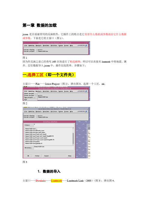
第一章数据的加载jason是目前最常用的反演软件,它操作上的特点是它需要什么数据或参数就给它什么数据或参数。
下面是它的主窗口(图1)。
图1因为作反演之前已经将坨163区块进行了构造解释,所以可以直接从lanmark中将地震、测井、层位数据导入jason中,操作比较简单。
步骤如下:一,选择工区(即一个文件夹)主窗口——File——Select Project(图2),弹出图3。
选择一个工区,ok。
图2图31. 数据的导入主窗口——Datalinks——Landmark——Landmark Link(2003)(图3),弹出图4。
图3图42. 工区的选择File——Seisworks project:选地震工区t163,ok。
(图5)图5File——Openworks project——选SHNEGCAI, 选井列表t163,ok。
(图5)此时,图5 窗口的状态栏将会发生变化,以上选择的工区将会显示。
(图6)图63. 地震数据的导入Select——Import——Seismic/property data(图7),弹出图8。
选cb 3dv(纯波数据,作反演时一定要用纯波数据),ok。
图7图84. 层位数据的导入Select——Import——Horizons,选择反演时需要的层位和断层(图9)。
图95. 井数据的导入Select(图7)——wells,弹出图10。
选择需要的井,ok。
图10E:Transport——Import,以上所选的landmark中的数据将传入jason中。
图11第二章合成记录的建立在jason上建合成记录的特点是精度高,但随意性大。
建立合成记录的步骤是:井曲线、地震数据、子波的加载,子波的编辑和评价,合成记录的生成和编辑。
1. 井曲线、地震数据、子波的输入主窗口——Analysis——Well log editing and seismic tie(图1),弹出图2。
图1图2Input——well,选择要输入的井,例如:T714_e。
Jason 软件详细介绍与基本操作手册
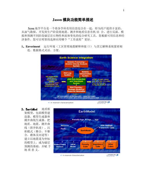
Jason模块功能简单描述Jason地学平台是一个将各学科有用信息综合在一起,即为用户提供丰富的、从油气勘探、开发到生产阶段将地震、测井和地质信息有机结合,进行反演、模拟和预测不同阶段储层岩石物性和流体变化的综合研究工具。
您根据可用信息和经济条件,您可以明智的选择应用哪个“工作流程”更好。
1、Enveriment 运行环境(工区管理地震解释和接口)与其它解释系统紧密相连、数据格式灵活、方便。
2、EarthMod 地质框架模型,包括模型建造器,模型生成器和测井曲线生成器。
把地质、地震、测井曲线(斜井轨迹)、沉积模式(整合,不整合,礁体及河道等)建立以地震道为坐标的模型上,成为储层预测的基础,并赋予地质意义。
3、VelMod 速度模型建立工具VelMod 除具有建立速度模型的基本功能外,且有其独特特征:•地质引导:结合地质信息进行插值运算,能把稀疏的速度数据拓展为三维速度场。
•基于地质概念的速度调整•真三维插值4 、Wavelets 二维和三维地震子波分析●无井、单井、多井提子波和空变子波分析●从斜井中进行真三维分析●估算信噪比谱●为使结果稳定利用模型驱动5、 Modtrace 完整的地震反演系统( 包括对大倾角地层)●所用约束稀疏脉冲反演是基于道的递归反演,产生地震带宽内的波阻抗数据。
●其算法的唯一特征应用解释控制,为获得可靠的低频信息提供工具。
在EarthMod 的基础上建立空变约束条件,其结果突出各向异性,提高了反演分辨率。
●多种方式提取子波,包括无井、单井多道、多井多道、直井、斜井提子波和在EarthMod 的基础上提空变子波。
●由于大量地震信息的反演是基于EarthMod 的基础,所以适用与多条复杂断层的地质情况,使其反演结果更接近真实的地质模型。
●给出产层有效厚度图和孔隙度分布图6、InverMod 精细储层描述(多井)•采用一欧洲石油公司的专利,专门致力于薄层预测和精细描述。
对油田滚动勘探开发十分有用。
SmacqDAQSoftware快速使用指南
Smacq DAQ Software 快速使用指南关于Smacq DAQ SoftwareSmacq DAQ Software是Smacq为USB-3000和USB-5000系列数据采集卡开发的数据采集软件。
Smacq DAQ Software可以帮助没有编程经验的用户快速获取实验数据。
Smacq DAQ Software的设计主要是针对基础应用,对于复杂应用需要用户根据实际情况选择合适的开发环境,编程实现相关功能。
Smacq提供多种环境的开发范例和说明文档,如有需要请到自行下载或与service@取得联系。
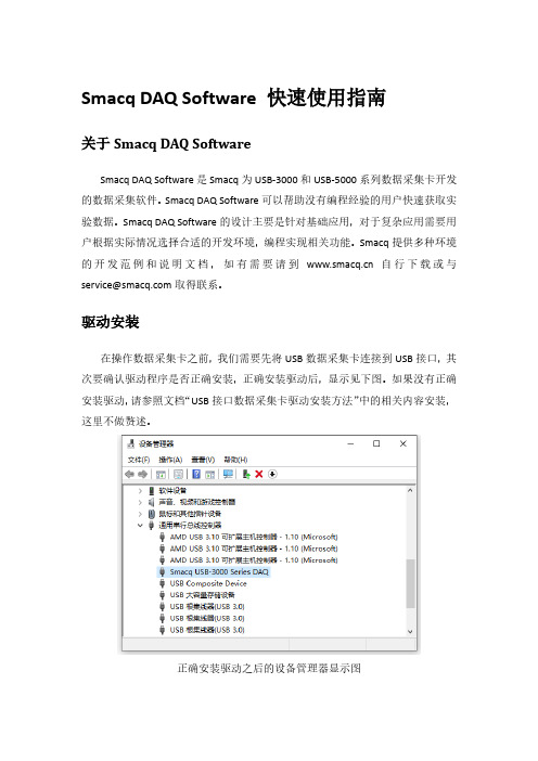
驱动安装在操作数据采集卡之前,我们需要先将USB数据采集卡连接到USB接口,其次要确认驱动程序是否正确安装,正确安装驱动后,显示见下图。
如果没有正确安装驱动,请参照文档“USB接口数据采集卡驱动安装方法”中的相关内容安装,这里不做赘述。
正确安装驱动之后的设备管理器显示图软件安装找到Smacq DAQ Softwave所在文件夹,双击运行setup.exe文件,一直下一步即可完成安装。
软件安装完成安装完成后,会在桌面创建快捷方式Smacq DAQ Softwave。
打开软件双击Smacq DAQ Software快捷方式打开软件。
打开软件后,点击Device List 按键,会在界面左侧显示连接到该电脑上的所有USB-3000和USB-5000系列数据采集卡的信息。
选择数据采集卡系列连接数据采集卡在设备选择列表中选择需要操作的采集卡,然后点击连接按键后,采集卡可以使用功能会激活。
连接数据采集卡功能说明Smacq DAQ Software有多种功能,详见下表。
YT模式采集卡连接后,点击YT按键,进入到YT模式。
YT模式是使用最多的功能,在YT模式中显示电压随时间变化的曲线。
在进行数据采集之前,需要选对采集卡进行设置。
YT模式模拟采集设置在YT模式中,点击设置进入YT-Config界面。
首先设置模拟输入的通道模式,根据硬件连接的方式进行选择,如果不清楚如果连接,可参考用户手册中3.2章节信号连接方式。
ThinkServer TS140 用户手册 V1.2

Jason手册a
前言JASON地学综合研究平台(JASON GEOSCIENCE WORKBENCH)为用户提供的跨越地震、地质、测井资料的综合分析研究工具,它可满足油气勘探开发不同阶段对储层的油气藏定量研究的需求。
JASON把不同学科的有效信息的融合作为客观存它的基石,最大限度地利用不同信息的优势,为用户提供符合不同学科信息的客观可靠的油气藏参数模型。
JASON软件的重要特点就是随着越来越多的非地震信息(测井、测试、地质)的引入,由地震数据推演的油气藏参数模型的分辩率和细节会得到不断的改善。
用户可根据需要,由JASON的模块构建自己的研究流程。
主要模块及功能如下:Enviaonment-Plus 运行环境及分析工具数据输入与输出(地震segy格式、测井las格式和层位ASCII格式)各种数据,各种方式的显示(井、层位、地震等的2D/3D显示)合成记录标定2D/3D解释(地震体与属性体解释)交会图/直方图分析三维立体显示与三维(地质/储集)体自动解释沿层、层间属性提取、沿层属性切片层位数据计算(平滑、加/减、拟合等)地层异常检测处理工具包(重采样、滤波、互相关等)等值线Wavelets 子波估算用多种技术估算地震子波(无井估算地震子波、单井或多井估算地震子波等)空变子波理论子波估算子波的振幅谱与相位谱计算平均子波VelMod 速度建模建立三维速度模型(用均方根速度,逐层的层速度编辑与平滑)时深转换,深时转换提供阻抗的低频模型EarthModel 地质框架模型构建以层为基础的地层框架模型生成以地层框架模型为基础的测井曲线内插模型提供用于地震反演的低频模型InverTrace 地震反演的储层与油气藏描述提供可靠的地震反演声阻抗数据体在地震反演声阻抗数据体上解释,可提高解释的精度和可靠性预测产层有效厚度和平均孔隙度InverMod 基于测井的精细储层油气藏描述StatMod 地质统计随机模拟与随机反演生成既满足测井资料和地质统计,又满足地震资料的储层/油气藏模型更准确地估算各种参数的不确定性,提供参数模拟的可靠性评定地质统计分析(直方图[油气藏参数的空间分布规律],变差图[油气藏参数的空间相关性])各种随机模拟与随机反演的算法:1.Sequential Gaussian Simulation (序贯高斯模拟)SGS2.Sequential Gaussian Collocated Co-simulation (序贯高斯配置协模拟) SGCCS3.Sequential Gaussian Co-simulation (序贯高斯协模拟) SGCS4.Sequential Indicator Simulation (序贯指示模拟,岩性模拟)SIS5. Lithology masks (遮挡岩性指示模拟)6.Sequential Indicator Simulation with a trend (带趋势的序贯指示模拟)SIS with trend7.Stochastic inversion (随机反演)8.Kriging/.CokrigingFunctionMod 数据分析变换工具Largo 测井曲线计算、正演与分析工具帮助用户分析测井曲线提供弹性反演所必须的横波测井资料提供利用测銰曲线判别流体的可靠准则RockTrace 弹性反演JASON (5.2)应用指南一、地震数据加载:3D道头 2D道头21 32 CDP number 21 32 CDP number13 32 line number 400 bytes line name73 32 X 73 32 X77 32 Y 77 32 Y109 32 first sample time 109 32 first sample time(一)3D磁盘文件加载(*.sgy):Datalinks → Seismic/Property data → SEG-Y → Disk SEG-Y Import …1、Parameters …1) Create/edit SEG-Y format definition …→Definition name →Standard disk SEG-YSEG-Y dimension → 3DSEG-Y disk mode → CQuick verify settings →File name → List …→选 SEG- Y 文件显示3200字节卷头显示240字节道头找到道头中的关键字节的位置,然后填写有关字节的位置:CDP →CDP ensemble number (offset 21) → 21Line number→ Specify trace header position below→ 221X coordinate → Source X-coornate (offset 73) → 73Y coordinate → Source Y -coornate (offset 73) → 77XY unit → Manual override → m……2) Select / edit transport parameters …(1) Segy format 在 list 中点按 (2) → us(3) Time gate1500 --- 3500 ms( 4) Time of first sample 0 ms(5) 3D→ 选 test.sgy 文件(7)点按→Survey name Trace selectionCDP’s在 list 中键入 内部文件名(10) UnitOk✓Floating pointOverwrite ✓pAppend and overwrite overlap ✓Append and don’t overwrite overlap2、Transport →Import selected files (即全部输入)3、 File → Save and Exit(自动生成三维工区平面图和地震数据文件seis.mod )(二)2D 磁盘文件(.sgy) 加载: (道头最好记录 CDP. X. Y…等信息)1、Parameters … (1) Select / edit transport parameters …步骤 1) 2) 3) 4) 同前5) 2D 2D lines → 选多个 *.sgy 文件给5) 一个个点亮 →--注意:2D 工区,如果道头没记 X.Y :!! 道头有X.Y ,加载省事,自动生成平面图和地震数据文件 seis.mod 。
MAXQDA 2022 入门指南 (简体中文)说明书

入门指南Free Guide简体中文 Chinese SimplifiedMAXQDA 2022 入门指南简体中文技术支持与销售:VERBI软件. 德国(柏林)社会研究咨询有限责任公司./china版权所有·侵权必究MAXQDA is a registered trademark of VERBI Software. Consult. Sozialforschung. GmbH,Berlin/Germany; Mac is a registered trademark of Apple Computer, Inc. in the United States and/or other countries; Microsoft Windows, Word, Excel, and PowerPoint are registered trademarks of Microsoft Corporation in the United States and/or other countries; SPSS is a registered trademark of IBM Corporation in the United States and/or other countries; Stata is a registered trademark of Stata Corp LLC. in the United States and/or other countries.All other trademarks or registered trademarks are the property of their respective owners, and may be registered in the United States and/or other jurisdictions.© VERBI软件. 德国(柏林)社会研究咨询有限责任公司. 2022目录 5目录目录 (5)引言 (7)MAXQDA概述 (8)项目启动 (8)用户界面 (9)有关数据存储和保存的几条说明 (11)重要概念 (12)数据输入和探索 (13)数据输入 (13)数据探索 (14)数据搜索 (17)颜色编码和备忘录 (18)数据编码 (20)数据片段编码 (20)数据分析 (23)文件激活 (23)检索使用相同代码编码的文件片段 (24)可视化的使用 (25)6混合方法分析的实施 (26)定义文件变量 (26)变量值的输入 (27)将代码频率转化为变量 (28)文件变量在分析中的使用 (29)推荐文献 (30)结束语 (31)引言7引言欢迎使用MAXQDA入门指南!鉴于当下几乎无人喜欢阅读冗长的介绍性文本或使用手册,我们努力为您提供一份尽可能精短的指南。
最新jason地质统计学反演手册资料讲解
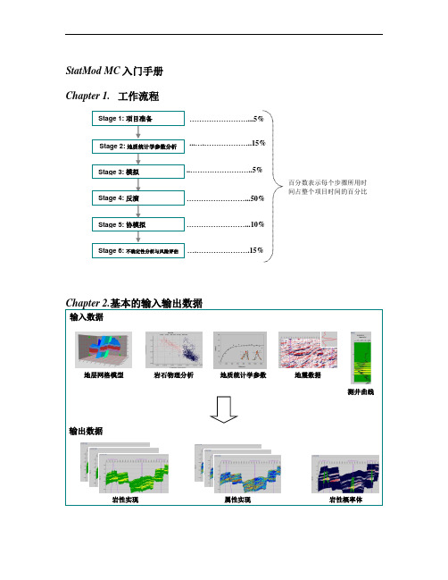
StatMod MC入门手册Chapter 1.工作流程Chapter 2.基本的输入输出数据输入数据输出数据岩性实现岩性概率体属性实现地质统计学参数岩石物理分析地层网格模型地震数据测井曲线……………………...5%...….………………..15%..……………………..5%……………………...50%……………………...10%….………………….15%百分数表示每个步骤所用时间占整个项目时间的百分比Stage 4:反演Stage 2:地质统计学参数分析Stage 3:模拟Stage 5:协模拟Stage 1: 项目准备Stage 6: 不确定性分析与风险评估Chapter 3.详细操作步骤操作步骤以StatMod MC培训数据为例第一步.首先完成一个高质量的叠后CSSI反演这一步的目的是为地质统计学提供一个好的研究基础, 这个“好”主要体现在:(1)好的井震标定, 目标区的相关值达到0.85以上;(2)好的叠后反演结果, 用来质控地质统计学模拟和反演结果, 是地质统计学反演结果横向预测准确度的参照物;(3)利用叠后反演结果进行砂体雕刻, 对目标区的岩性展布、比例有一个总体上正确的把握, 这些认识都是地质统计学的初始输入。
(说明:在提供的培训数据中已经为用户做了以上准备,用户可以从主界面中打开该培训数据所在工区, 然后用Map View看工区底图,用Section View查看地震数据、叠后CSSI反演数据、地质框架模型与层位数据以及井数据与子波 , 并用Well Editor检查井震标定情况)第二步. 数据准备●●井曲线重采样这一步将测井数据重采样至地质微层采样间隔,具体操作为:(1)JGW主界面→ Analysis→ Processing toolkit;(2)Input→ Data selection→ Data type:选Well, 点击Input file(s)右边List选择任意井(可以选多井),然后在弹出的界面Select logs中选择任意井曲线(可以多选),点击OK退出;(3)Parameters→ Resample log, 在弹出界面Processing toolkit中填写重采样间隔(注意s 与ms单位),点击OK退出;(4)Output→ Define process, 从Select from中选择Resample log, 点击››输入到右边的Process里面;(5)Output→ Generate, 在弹出的界面中填写输出路径和输出文件名,然后点击Generate,开始计算重采样的曲线。
青山资料软件操作手册 2
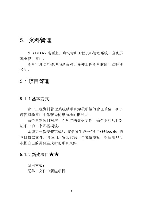
5. 资料管理在WINDOWS桌面上,启动青山工程资料管理系统一直到屏幕出现主窗口。
资料管理功能体现为系统对于各种工程资料的统一维护和控制。
5.1项目管理5.1.1基本方式青山工程资料管理系统以项目为最顶级的管理单位,在资源管理器窗口中体现为树形结构的根节点。
每个资料项目对应一个独立的数据文件,每个资料项目对应唯一的一个表格模板。
系统第一次安装完成后,将缺省生成一个叫“office.db”的项目数据文件,对应用户安装的第一个表格模板。
以后用户可根据自己的需要生成新的项目文件。
5.1.2新建项目★★调用方式:菜单->文件->新建项目功能说明:创建一个新的项目文件进行资料编制。
首先指定存放项目的数据文件:为项目文件指定名称及存放目录,如果指定的项目文件名称在存放目录中已经存在,系统会提示是否替换已有文件:为数据安全起见,一般不要替换原有项目文件。
项目文件创建成功后,如果当前项目有打开的工程资料,系统会自动关闭这些资料并提示保存已经修改的工程资料。
然后提示用户选择资料体系与合适的表格模板相关联。
如果用户只安装了唯一的表格模板,将不会出现该提示。
5.1.3打开项目调用方式:菜单->文件->打开项目菜单->文件->最近文件列表功能说明:打开一个已有的项目文件进行资料编制。
最近文件列表是最近使用的4个项目文件名称列表。
在文件菜单的底部,由系统自动维护,方便快速开启最近使用项目。
系统重新运行时会自动打开上一次运行时最后使用的项目文件。
5.1.4同步项目★调用条件:当前活动窗口为列表窗口。
调用方式:菜单->文件->同步项目功能说明:资料模板勘误升级后,如果资料数量有所增减,需要使用该功能升级已经建立好的项目文件。
5.1.5设置项目信息★★★调用条件:当前活动窗口为列表窗口。
调用方式:资源管理器->根目录按鼠标右键->项目信息功能说明:设置隶属于项目的相关重要信息。
SeisMod 4.0使用手册(下)

第二部分波动方程正演模拟软件建模与运行1. 概述 (4)1.1 模型建立器(Model Builder) (4)1.1.1 地质参数模型建模方法 (5)1.1.2 模型建立器功能及特点 (5)1.2 地震波场正演模拟引擎(Modeling Engine) (6)1.2.1 多种介质模型地震波波动方程 (6)1.2.2 正演模拟引擎的功能及特点 (7)2. SeisMod用户界面 (8)2.1 SeisMod软件的启动 (8)2.2 SeisMod软件界面组成 (9)2.2.1 菜单条 (9)2.2.2 垂直尺和水平尺 (11)2.2.3 图形客户区 (11)3. 地质参数模型建立 (12)3.1 地质模型设计 (12)3.1.1 地质模型设计方式一 (12)3.1.2 地质模型设计方式二 (17)3.1.3 地质模型设计方式三 (18)3.1.4 地质模型修改 (19)3.2 保存地质模型 (22)3.3 加载地质模型 (22)3.4 删除地质模型 (23)3.5 输入地质模型 (24)3.6 输出地质模型 (24)4. 模型网格化 (26)4.1 层参数定义网格化 (26)4.2 测井曲线定义网格化 (28)4.2.1 将井投影到地质模型上 (28)4.2.2 加载测井曲线 (28)4.2.3 编辑控制曲线 (28)4.2.4 曲线外推模型网格化 (29)4.2.5 保存网格地质参数模型 (29)5. 地震波场正演模拟 (31)5.1 地质参数模型 (31)5.1.1 网格地质参数模型的模型参数 (31)5.1.2 矢量地质参数模型的模型参数 (32)5.2 观测系统定义 (33)5.2.1 叠加剖面模拟 (34)5.2.2 多次覆盖观测系统的定义 (34)5.2.3 VSP观测系统的定义 (35)5.2.4 井间观测系统的定义 (36)6. 照明分析 (37)6.1 照明计算 (37)6.2 显示照明分析结果 (38)6.3 删除照明分析结果 (38)7. 地震数据浏览器 (40)7.1 显示地震数据 (40)7.2 地震数据显示风格 (41)7.2.1 单色显示风格 (41)7.2.2 彩色显示风格 (45)7.2.3 混合显示风格 (48)8. 叠后波动方程偏移 (48)2北京恒泰艾普石油勘探开发技术有限公司SeisMod使用手册31. 概述地震波正演模拟是研究地球介质中地震波传播的运动学和动力学特征的重要手段,也是地震资料偏移成像的基础。
DAMS软件使用手册
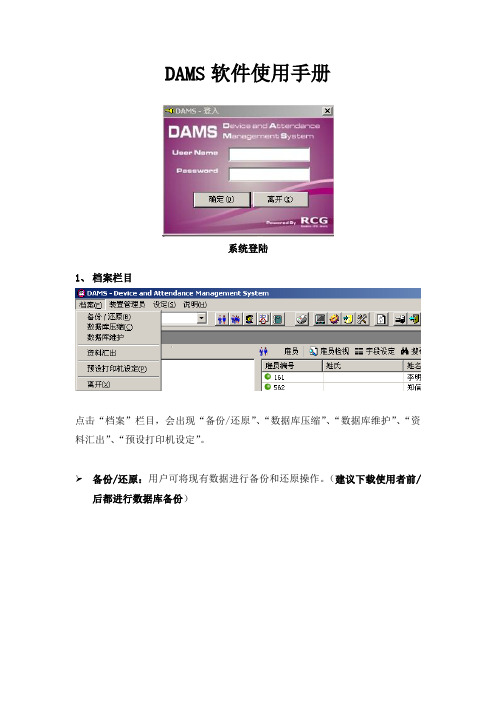
DAMS软件使用手册系统登陆1、档案栏目点击“档案”栏目,会出现“备份/还原”、“数据库压缩”、“数据库维护”、“资料汇出”、“预设打印机设定”。
备份/还原:用户可将现有数据进行备份和还原操作。
(建议下载使用者前/后都进行数据库备份)数据库压缩:用户可以对数据库进行压缩,以减小数据库使用硬盘的存储量。
资料汇出:用户可以将“雇员主要资料”和“已分析的考勤记录”以EXCEL 方式进行汇出。
数据库维护:可手动对数据进行删除操作。
2、装置管理员栏目点击“装置管理员”将出现如下界面:新增考勤机:新增加考勤机并对其进行配置名称:随意填写型号:I4 Flexi装置编号:一定与前台考勤机设置一样IP地址:一定与前台考勤机设置一样修改:对选择的考勤机配置进行修改。
移除考勤机:将选择的考勤机进行删除操作。
选择所有:一次性选择所有考勤机。
选择取消:取消所有选择的考勤机。
下载:将选择的考勤机的考勤记录下载到本地(注意:下载成功后考勤机的考勤记录会自动删除)。
预设下载:用户可以设置一个时间段,让系统自动下载考勤记录。
时间同步:将服务器时间同步到前端考勤机。
传送时区:将预先设置好的时区(时区的定义:规定在某个时间段内才是有效的考勤时间)上载到考勤机内。
下载使用者:在指纹考勤系统运行中,如果某台考勤机有新用户的指纹信息添加或有用户的指纹信息做了修改后,需要对本台考勤机进行此操作。
上载使用者:若添加了新的考勤机或进行了下载使用者操作后,需要对其他考勤机进行指纹数据同步时,进行此操作。
(注意:此操作会将考勤机现有的所有指纹数据进行覆盖)将需要编排在同一个组的考勤设备进行编组。
点击使用者后出现如下界面:(带*号的证明该用户已经有指纹数据)时间表编号:是用户设置好的时区内的有效考勤时间段,选择了时间表编号后代表使用者只有在规定的时间段才是有效考勤时间,其余时间段为无效考勤时间。
设置有效考勤时间段,每个时区可设置4个有效考勤时间段(如果用户在验证指纹时,考勤机提示“验证拒绝”,代表此是时间不是有效考勤时间)3、设定栏目点击“设定”栏目,会出现“公司资料”、“使用者设定”、“部门”、“工作群组”、“员工记录”、“工作时间表”、“选项”。
MultiTest 软件用户手册 V2.0
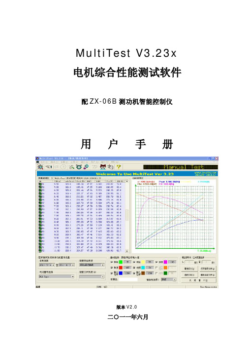
MultiTest V3.23x 电机综合性能测试软件配ZX-06B测功机智能控制仪用户手册版本V2.0二○一一年六月目录一、概述 (3)二、手动测试 (3)三、自动测试 (6)四、定点/耐久(FFU)/堵转测试 (11)五、系统参数设置 (15)六、量程设置,转矩单位 (16)七、串口设置 (16)八、转矩静态校准 (17)九、用户注册 (18)十、用户管理和更改密码 (19)十一、用户登录 (19)十二、数据/曲线查询 (20)一、概述MultiTest V3.23x电机综合性能测试软件是在Microsoft公司的Visual C++6.0开发环境下编制而成的,采用耳目一新的测试界面,具有良好的人机交互环境。
配合本公司的最新产品ZX-06B测功机智能控制仪,两者相结合所产生的测试功能,能够满足当前绝大多数厂家对其不同品种,不同型号电机的各种测试需求。
本软件还可选配DR4615转矩转速显示仪,DC4619控制仪或DR4615A电机性能测试仪(三合一)。
同时,电参数仪还可匹配8716B、PF100系列交流电参数仪,8716F、PF200直流电参数仪,8902F、PF300系列三相电参数仪,8760F电机寿命测控仪等。
也可以根据客户的要求匹配各个不同厂家,不同型号的电参数仪,多路带电绕阻温升仪。
还可以根据客户自身的特殊需求为其专门定制新功能。
测试软件新特性:1、耳目一新的测试界面,良好的人机交互环境。
2、采用自身定制的串口类调用Windows底层API函数实现串口通讯,而不是采用OCX控件。
3、所有采样均放在线程中进行,速度快,受干扰小。
而其它公司的测试软件都将采样放在主进程中进行。
4、可控制数量最多达到三台的测功机同时进行测试,在减少了企业人力资源的同时极大的提高了工作效率。
5、电机测试数据均按测试日期及电机型号进行分类归档,方便查询。
测试方式分为三种:手动测试,自动测试,定点/耐久(FFU)/堵转测试,以下分别加以详细介绍。
TMSURVIV 生存分析软件用户手册说明书
TMSURVIVUser's ManualbyJames E. HinesBiological Resources Division, USGS(1)11510 American Holly Dr. #201Patuxent Wildlife Research CenterLaurel, MD 20708-4017email: jim_hines%IntroductionProgram TMSURVIV (Transient-Model-SURVIV al analysis) computes parameter estimates of survival and capture probability and proportions of "residents" under the Jolly-Seber models described in "Capture-Recapture Survival Models Taking Account of Transients" (Pradel et. al., 1997). Actually, TMSURVIV is a specially modified version of Dr. G. White's program SURVIV (White, 1983) which incorporates the transient models. With this program and it's companion program, CNVTMSRV, users are able to get parameter estimates for these complex models from capture-history data without having to specify the cell probabilities.TMSURVIV is intended to be used in a situation where the sampling area includes animals which pass through the area and are not part of the "resident" population. .Output from TMSURVIV includes survival probability estimates, capture probability estimates, estimates of the proportion of residents, goodness-of-fit tests, and likelihood-ratio tests.By default, models are generated for standard Jolly-Seber models (where all animals are assumed to be residents), and transient models (a portion of the population is transient and only available for capture in one sample). The model names signify the structure of the model. Each model name is in the form "S.P.G." where "S" stands for survival, "P" stands for capture probability, and "G" stands for "gamma (proportion of residents)". If S,P, or G are followed by a "t", then the corresponding parameter is "time-dependent". If there is no "G" in the name, then all animals are assumed to be residents (proportion of residents = 1.0), which is equivalent to the Jolly-Seber models.Since program TMSURVIV is a generalization of program JOLLY, the conversion/model generation program (CNVTMSRV) will read input files designed for program JOLLY. Input consists of capture-histories for each animal, preceded by statements defining the specifics of the data (title, number of periods, interval lengths).Using CNVTMSRVTo run CNVTMSRV, type CNVTMSRV at the DOS prompt and respond to the program prompts. When the program is run, you are prompted for the name of the file(s) containing the capture-histories. Analysis on groups of animals may be performed by separating the capture-histories into different files. CNVTMSRV will prompt for each input file and a 1-character identifier (eg. M for male, F for female) until 'END' is entered for the input file.Here is the output file created by CNVTMSRV which can be input to TMSURVIV:PROC TITLE 'Lazuli bunting data from DESIGN & ANAL. METH... Burhnam et al.';PROC MODEL NPAR=21 ADDCELL;COHORT= 168 /* unmarked in 1 */;31:; 4:; 0:; 1:; 0:; 0:; 0:;COHORT= 31 /* marked in 2 */;7:; 4:; 0:; 0:; 0:; 0:;COHORT= 367 /* unmarked in 2 */;12:; 10:; 4:; 1:; 0:; 1:;COHORT= 23 /* marked in 3 */;12:; 0:; 1:; 0:; 0:;COHORT= 65 /* unmarked in 3 */;8:; 3:; 0:; 0:; 0:;COHORT= 34 /* marked in 4 */;16:; 3:; 0:; 0:;COHORT= 230 /* unmarked in 4 */;25:; 3:; 3:; 1:;COHORT= 49 /* marked in 5 */;20:; 0:; 0:;COHORT= 255 /* unmarked in 5 */;38:; 13:; 1:;COHORT= 66 /* marked in 6 */;28:; 2:;COHORT= 256 /* unmarked in 6 */;39:; 7:;COHORT= 83 /* marked in 7 */;30:;COHORT= 240 /* unmarked in 7 */;46:;LABELS;S(1)=PHI(1);S(2)=PHI(2);S(3)=PHI(3);S(4)=PHI(4);S(5)=PHI(5);S(6)=PHI(6);S(7)=PHI(7);S(8)=p(2);S(9)=p(3);S(10)=p(4);S(11)=p(5);S(12)=p(6);S(13)=p(7);S(14)=p(8);S(15)=gamma(1);S(16)=gamma(2);S(17)=gamma(3);S(18)=gamma(4);S(19)=gamma(5);S(20)=gamma(6);S(21)=gamma(7);PROC ESTIMATE NOVAR MAXFN=32000 NAME=SP; CONSTRAINTS; S(2)=S(1);S(3)=S(1);S(4)=S(1);S(5)=S(1);S(6)=S(1);S(7)=S(1);S(9)=S(8);S(10)=S(8);S(11)=S(8);S(12)=S(8);S(13)=S(8);S(14)=S(8);S(15)=1;S(16)=1;S(17)=1;S(18)=1;S(19)=1;S(20)=1;S(21)=1;PROC ESTIMATE NOVAR MAXFN=32000 NAME=SPG; CONSTRAINTS; S(2)=S(1);S(3)=S(1);S(4)=S(1);S(5)=S(1);S(6)=S(1);S(7)=S(1);S(9)=S(8);S(10)=S(8);S(11)=S(8);S(12)=S(8);S(13)=S(8);S(14)=S(8);S(16)=S(15);S(17)=S(15);S(18)=S(15);S(19)=S(15);S(20)=S(15);S(21)=S(15);PROC ESTIMATE NOVAR MAXFN=32000 NAME=StPt; CONSTRAINTS; S(16)=1;S(17)=1;S(18)=1;S(19)=1;S(20)=1;S(21)=1;PROC ESTIMATE NOVAR MAXFN=1 NAME=StPtGt; CONSTRAINTS; S(14)=1;S(15)=1;initial;s(1)=0.588756 ;s(2)=0.480049 ;s(3)=0.727235 ;s(4)=0.601595 ;s(5)=0.608575 ;s(6)=0.501442 ;s(7)=0.349755 ;s(8)=0.313413 ;s(9)=0.454870 ;s(10)=0.655431 ;s(11)=0.688543 ;s(12)=0.629337 ;s(13)=0.737137 ;s(16)=0.168890 ;s(17)=0.214131 ;s(18)=0.286596 ;s(19)=0.364735 ;s(20)=0.453364 ;s(21)=0.562283 ;PROC TEST; PROC STOP;The output file, CNVTMSRV.OUT, contains a title statement, statements to define the input data, label definitions, statements to describe models, a test statement and a stop statement.The title statement is used to identify the data used in the analysis.The model definition statements start with "PROC MODEL NPAR=21 ADDCELL;" and end with "COHORT=240;". The "NPAR=21" indicates the maximum number of parameters (estimated or fixed) in any of the following models. In this example there are 7 survival rate parameters, 7 capture probability parameters, and 7 residency parameters.Following the data are the labels for each of the parameters. Internally, the parameters are called"S(1), S(2), ... S(NPAR). The labels relate these internal parameters to meaningful labels for these models. The survival parameters are labelled PHI, followed by time period in parenthesis. The capture-probability parameters are labelled "p", and the residency parameters are labelled "gamma". If more than one group was input, the label will have a 1-character identifier tacked onto the end to indicate the group.After the label definitions come the model definitions for each model. Each model starts with a "PROC ESTIMATE" statement. Options on the "PROC ESTIMATE" statement include "NOVAR" which inhibits printing of the variance-covariance matrix, the number of significant digits, "NSIG" (i.e., number of digits following the decimal point which do not change at the end of the iterative process), the maximum number of function evaluations, "MAXFN", and the name of the model. If the variance-covariance matrix of parameter estimates is desired, delete the string "NOVAR" using a text editor.CNVTMSRV produces the model definitions from most restrictive (model "SP") to most general (model "StPtGt"). The reason for this is that the most restrictive model has the fewest estimable parameters and converges more easily. Final estimates from this model can then be input as starting values to more general models. If more than one group was entered in CNVTMSRV, a series of additional models is produced which assumes the data came from only one group (eg. 1SP, 1StPtGt,...).The statements following the "CONSTRAINTS" statement describe each model in terms of the most general model. In model "SP", the survival and capture probabilities are assumed to be constant across time, so the survival probabilities for time period two and three are set equal to the survivalprobabilities for time period one. The capture probabilities are also assumed constant over time, so the capture probabilities for time periods 3 and 4 are set equal to the capture probabilities for time period 2. These equalities must be specified in terms of parameter number which can be obtained from the labels section.The sequence of statements starting with "PROC ESTIMATE ... NAME=SPG" cause TMSURVIV to produce estimates under the model with constant survival and capture probabilities and a constant proportion of residents.The sequence of statements starting with "PROC ESTIMATE ... NAME=StP" cause TMSURVIV to produce estimates under the model with time-specific survival probabilities and constant capture probabilities (equivalent to model "B" in JOLLY).The "PROC TEST;" statement causes TMSURVIV to print tables of statistics used for comparison of the models. "PROC STOP;" causes TMSURVIV to stop execution even if more statements follow. TMSURVIVTMSURVIV prompts for one line of input to specify the name of the input and output files and command line options. When the program is run, the following prompt appears:Enter command line parameters [i=in_file] [l=out_file][lines=n] [compile run] [noecho]:At this prompt, any or all of the items enclosed in brackets may be specified. If "i=in_file" is specified, the input will be read from the file "in_file". Usually, this is the file created by CNVTMSRV and is called CNVTMSRV.OUT unless it has been renamed. A full pathname may be used to indicate a different directory. If this item is omitted, TMSURVIV expects the input from the keyboard. (Cntl-Break will abort the program).If "l=out_file" is specified, output from TMSURVIV will be directed to the file "out_file". The default output file is the CRT screen. To direct output directly to the printer, use "l=lpt1".If "lines=n" is included, TMSURVIV will print a header and the title in the output file after every n lines. The default value for n is 60.If "compile run" is included, TMSURVIV will only check the input file for errors and not perform any analysis. This option is used in SURVIV to create the estimation routine and is not needed in TMSURVIV.The "noecho" option causes TMSURVIV to suppress printing of the input data. This option is useful when there are several runs of models on the same data and you would like to conserve paper, but at least one run should contain a listing of the data to check for "typos".To run the sample data file with TMSURVIV, enter the following at the above prompt:i=cnvtmsrv.out l=sample.out lines=9999The output produced by TMSURVIV contains a listing of the input data, estimates of the parameters under each model, a goodness-of-fit test for each model, an AIC statistic for each model, and between model tests. The following output was created using TMSURVIV on the sample data file listed previously:SURVIV - Survival Rate Estimation with User Specified Cell Probabilities2-Sep-97 15:47:55 Version 1.4(OS/2) June, 1991 Page 001INPUT --- PROC TITLE 'Lazuli bunting data from DESIGN & ANAL. METH...INPUT --- Burhnam et al.';CPU time in seconds for last procedure was 0.00INPUT --- PROC MODEL NPAR=21 ADDCELL;INPUT --- COHORT= 168 /* unmarked in 1 */;INPUT --- 31:;4:;0:;1:;0:;0:;0:;INPUT --- COHORT= 31 /* marked in 2 */;INPUT --- 7:;4:;0:;0:;0:;0:;INPUT --- COHORT= 367 /* unmarked in 2 */;INPUT --- 12:;10:;4:;1:;0:;1:;INPUT --- COHORT= 23 /* marked in 3 */;INPUT --- 12:;0:;1:;0:;0:;INPUT --- COHORT= 65 /* unmarked in 3 */;INPUT --- 8:;3:;0:;0:;0:;INPUT --- COHORT= 34 /* marked in 4 */;INPUT --- 16:;3:;0:;0:;INPUT --- COHORT= 230 /* unmarked in 4 */;INPUT --- 25:;3:;3:;1:;INPUT --- COHORT= 49 /* marked in 5 */;INPUT --- 20:;0:;0:;INPUT --- COHORT= 255 /* unmarked in 5 */;INPUT --- 38:;13:;1:;INPUT --- COHORT= 66 /* marked in 6 */;INPUT --- 28:;2:;INPUT --- COHORT= 256 /* unmarked in 6 */;INPUT --- 39:;7:;INPUT --- COHORT= 83 /* marked in 7 */;INPUT --- 30:;INPUT --- COHORT= 240 /* unmarked in 7 */;INPUT --- 46:;INPUT --- PROC ESTIMATE NOVAR MAXFN=32000 NAME=SP;Number of parameters in model = 21Number of parameters set equal = 12Number of parameters fixed = 7Number of parameters estimated = 2Final function value 1133.1718 (Error Return = 0)Number of significant digits 7Number of function evaluations 4595% Confidence Interval I Parameter S(I) Standard Error Lower Upper --- -------------------- ------------ ------------ ------------ ------------1 1 PHI(1) 0.379861 0.200672E-01 0.340529 0.4191932 1 PHI(2) 0.379861 0.200672E-01 0.340529 0.4191933 1 PHI(3) 0.379861 0.200672E-01 0.340529 0.4191934 1 PHI(4) 0.379861 0.200672E-01 0.340529 0.4191935 1 PHI(5) 0.379861 0.200672E-01 0.340529 0.4191936 1 PHI(6) 0.379861 0.200672E-01 0.340529 0.4191937 1 PHI(7) 0.379861 0.200672E-01 0.340529 0.4191938 2 p(2) 0.432594 0.327044E-01 0.368494 0.4966959 2 p(3) 0.432594 0.327044E-01 0.368494 0.49669510 2 p(4) 0.432594 0.327044E-01 0.368494 0.49669511 2 p(5) 0.432594 0.327044E-01 0.368494 0.49669512 2 p(6) 0.432594 0.327044E-01 0.368494 0.49669513 2 p(7) 0.432594 0.327044E-01 0.368494 0.49669514 2 p(8) 0.432594 0.327044E-01 0.368494 0.49669515 -15 gamma(1) 1.00000 0.000000E+00 1.00000 1.0000016 -16 gamma(2) 1.00000 0.000000E+00 1.00000 1.0000017 -17 gamma(3) 1.00000 0.000000E+00 1.00000 1.0000018 -18 gamma(4) 1.00000 0.000000E+00 1.00000 1.0000019 -19 gamma(5) 1.00000 0.000000E+00 1.00000 1.0000020 -20 gamma(6) 1.00000 0.000000E+00 1.00000 1.0000021 -21 gamma(7) 1.00000 0.000000E+00 1.00000 1.00000 Cohort Cell Observed Expected Chi-square Note------ ---- -------- -------- ---------- -------------1 1 31 27.607 0.417 0 < P < 11 2 4 5.950 0.639 0 < P < 11 3 0 1.282 1.282 0 < P < 11 4 1 0.276 1.894 0 < P < 11 5 0 0.060 0.060 0 < P < 11 6 0 0.013 0.013 0 < P < 11 7 0 0.003 0.003 0 < P < 11 8 132 132.809 0.005 0 < P < 11 Cohort df=2 1.303 P = 0.52142 1 7 5.094 0.713 0 < P < 12 2 4 1.098 7.670 0 < P < 12 3 0 0.237 0.237 0 < P < 12 4 0 0.051 0.051 0 < P < 12 5 0 0.011 0.011 0 < P < 12 6 0 0.002 0.002 0 < P < 12 7 20 24.507 0.829 0 < P < 12 Cohort df= 1 3.957 P = 0.04673 1 12 60.308 38.695 0 < P < 13 2 10 12.998 0.692 0 < P < 13 34 2.802 0.513 0 < P < 13 4 1 0.604 0.260 0 < P < 13 5 0 0.130 0.130 0 < P < 13 6 1 0.028 33.676 0 < P < 13 7 339 290.130 8.232 0 < P < 13 Cohort df= 3 49.284 P = 0.00004 1 12 3.779 17.880 0 < P < 14 2 0 0.815 0.815 0 < P < 14 3 1 0.176 3.871 0 < P < 14 4 0 0.038 0.038 0 < P < 14 5 0 0.008 0.008 0 < P < 14 6 10 18.184 3.684 0 < P < 14 Cohort df= 1 17.593 P = 0.00005 1 8 10.681 0.673 0 < P < 15 2 3 2.302 0.212 0 < P < 15 3 0 0.496 0.496 0 < P < 15 4 0 0.107 0.107 0 < P < 15 5 0 0.023 0.023 0 < P < 15 6 54 51.390 0.133 0 < P < 15 Cohort df= 2 0.807 P = 0.66796 1 16 5.587 19.407 0 < P < 16 2 3 1.204 2.678 0 < P < 16 3 0 0.260 0.260 0 < P < 16 4 0 0.056 0.056 0 < P < 16 5 15 26.893 5.260 0 < P < 16 Cohort df= 1 25.163 P = 0.00007 1 25 37.795 4.332 0 < P < 17 2 3 8.146 3.251 0 < P < 17 3 3 1.756 0.882 0 < P < 17 4 1 0.378 1.021 0 < P < 17 5 198 181.925 1.420 0 < P < 17 Cohort df= 3 10.634 P = 0.01398 1 20 8.052 17.729 0 < P < 18 2 0 1.735 1.735 0 < P < 18 3 0 0.374 0.374 0 < P < 18 4 29 38.838 2.492 0 < P < 18 Cohort df= 2 22.331 P = 0.00009 1 38 41.903 0.364 0 < P < 19 2 13 9.032 1.744 0 < P < 19 3 1 1.947 0.460 0 < P < 19 4 203 202.119 0.004 0 < P < 19 Cohort df= 2 1.199 P = 0.549010 1 28 10.846 27.134 0 < P < 110 2 2 2.338 0.049 0 < P < 110 3 36 52.817 5.355 0 < P < 110 Cohort df= 2 32.537 P = 0.000011 1 39 42.067 0.224 0 < P < 111 2 7 9.067 0.471 0 < P < 111 3 210 204.866 0.129 0 < P < 111 Cohort df= 2 0.824 P = 0.662512 1 30 13.639 19.626 0 < P < 112 2 53 69.361 3.859 0 < P < 112 Cohort df= 1 23.485 P = 0.000013 1 46 39.438 1.092 0 < P < 113 2 194 200.562 0.215 0 < P < 113 Cohort df= 1 1.306 P = 0.2530------------------------------------------------------------@@ 1 0 0 47 207.123 21 190.424 -157.121 318.242G Total (Degrees of freedom = 47) 207.123Pr(Larger Chi-square) = 0.0000With pooling, Degrees of freedom = 21 Pearson Chi-square = 190.424Pr(Larger Chi-square) = 0.0000Log-likelihood = -157.12123 Akaike Information Criterion = 318.24245 CPU time in seconds for last procedure was 0.03INPUT --- PROC ESTIMATE NOVAR MAXFN=32000 NAME=SPG;Number of parameters in model = 21Number of parameters set equal = 18Number of parameters fixed = 0Number of parameters estimated = 3Final function value 1081.9256 (Error Return = 0)Number of significant digits 8Number of function evaluations 7195% Confidence IntervalI Parameter S(I) Standard Error Lower Upper --- -------------------- ------------ ------------ ------------ ------------1 1 PHI(1) 0.586343 0.291084E-01 0.529291 0.6433962 1 PHI(2) 0.586343 0.291084E-01 0.529291 0.6433963 1 PHI(3) 0.586343 0.291084E-01 0.529291 0.6433964 1 PHI(4) 0.586343 0.291084E-01 0.529291 0.6433965 1 PHI(5) 0.586343 0.291084E-01 0.529291 0.6433966 1 PHI(6) 0.586343 0.291084E-01 0.529291 0.6433967 1 PHI(7) 0.586343 0.291084E-01 0.529291 0.6433968 2 p(2) 0.617879 0.328420E-01 0.553509 0.6822509 2 p(3) 0.617879 0.328420E-01 0.553509 0.68225010 2 p(4) 0.617879 0.328420E-01 0.553509 0.68225011 2 p(5) 0.617879 0.328420E-01 0.553509 0.68225012 2 p(6) 0.617879 0.328420E-01 0.553509 0.68225013 2 p(7) 0.617879 0.328420E-01 0.553509 0.68225014 2 p(8) 0.617879 0.328420E-01 0.553509 0.68225015 3 gamma(1) 0.354799 0.316262E-01 0.292812 0.41678616 3 gamma(2) 0.354799 0.316262E-01 0.292812 0.41678617 3 gamma(3) 0.354799 0.316262E-01 0.292812 0.41678618 3 gamma(4) 0.354799 0.316262E-01 0.292812 0.41678619 3 gamma(5) 0.354799 0.316262E-01 0.292812 0.41678620 3 gamma(6) 0.354799 0.316262E-01 0.292812 0.41678621 3 gamma(7) 0.354799 0.316262E-01 0.292812 0.416786 Cohort Cell Observed Expected Chi-square Note------ ---- -------- -------- ---------- -------------1 1 31 21.595 4.096 0 < P < 11 2 4 4.838 0.145 0 < P < 11 3 0 1.084 1.084 0 < P < 11 4 1 0.243 2.360 0 < P < 11 5 0 0.054 0.054 0 < P < 11 6 0 0.012 0.012 0 < P < 11 7 0 0.003 0.003 0 < P < 11 8 132 140.171 0.476 0 < P < 11 Cohort df=2 4.817 P = 0.08992 1 7 11.231 1.594 0 < P < 12 2 4 2.516 0.875 0 < P < 12 3 0 0.564 0.564 0 < P < 12 4 0 0.126 0.126 0 < P < 12 5 0 0.028 0.028 0 < P < 12 6 0 0.006 0.006 0 < P < 12 7 20 16.528 0.729 0 < P < 12 Cohort df= 2 2.501 P = 0.28643 1 12 47.174 26.227 0 < P < 13 2 10 10.570 0.031 0 < P < 13 34 2.368 1.124 0 < P < 13 4 1 0.531 0.415 0 < P < 13 5 0 0.119 0.119 0 < P < 13 6 1 0.027 35.570 0 < P < 13 7 339 306.212 3.511 0 < P < 13 Cohort df= 3 32.638 P = 0.00004 1 12 8.333 1.614 0 < P < 14 2 0 1.867 1.867 0 < P < 14 3 1 0.418 0.809 0 < P < 14 4 0 0.094 0.094 0 < P < 14 5 0 0.021 0.021 0 < P < 14 6 10 12.267 0.419 0 < P < 14 Cohort df= 2 2.850 P = 0.24055 1 8 8.355 0.015 0 < P < 15 2 3 1.872 0.680 0 < P < 15 3 0 0.419 0.419 0 < P < 15 4 0 0.094 0.094 0 < P < 15 5 0 0.021 0.021 0 < P < 15 6 54 54.238 0.001 0 < P < 15 Cohort df= 2 0.163 P = 0.92196 1 16 12.318 1.101 0 < P < 16 2 3 2.760 0.021 0 < P < 16 3 0 0.618 0.618 0 < P < 16 4 0 0.139 0.139 0 < P < 16 5 15 18.165 0.552 0 < P < 16 Cohort df= 2 1.728 P = 0.42147 1 25 29.564 0.705 0 < P < 17 2 3 6.624 1.983 0 < P < 17 3 3 1.484 1.548 0 < P < 17 4 1 0.333 1.340 0 < P < 17 5 198 191.995 0.188 0 < P < 17 Cohort df= 2 1.138 P = 0.56608 1 20 17.752 0.285 0 < P < 18 2 0 3.977 3.977 0 < P < 18 3 0 0.891 0.891 0 < P < 18 4 29 26.379 0.260 0 < P < 18 Cohort df= 2 5.414 P = 0.06689 1 38 32.778 0.832 0 < P < 19 2 13 7.344 4.356 0 < P < 19 3 1 1.645 0.253 0 < P < 19 4 203 213.233 0.491 0 < P < 19 Cohort df= 2 4.116 P = 0.127710 1 28 23.911 0.699 0 < P < 110 2 2 5.357 2.104 0 < P < 110 3 36 36.732 0.015 0 < P < 110 Cohort df= 2 2.818 P = 0.244411 1 39 32.906 1.128 0 < P < 111 2 7 7.373 0.019 0 < P < 111 3 210 215.721 0.152 0 < P < 111 Cohort df= 2 1.299 P = 0.522312 1 30 30.070 0.000 0 < P < 112 2 53 52.930 0.000 0 < P < 112 Cohort df= 1 0.000 P = 0.987213 1 46 30.850 7.440 0 < P < 113 2 194 209.150 1.097 0 < P < 113 Cohort df= 1 8.538 P = 0.0035------------------------------------------------------------@@ 2 0 0 46 104.630 22 68.0196 -105.875 217.750G Total (Degrees of freedom = 46) 104.630Pr(Larger Chi-square) = 0.0000With pooling, Degrees of freedom = 22 Pearson Chi-square = 68.020Pr(Larger Chi-square) = 0.0000Log-likelihood = -105.87508 Akaike Information Criterion = 217.75016 CPU time in seconds for last procedure was 0.05INPUT --- PROC ESTIMATE NOVAR MAXFN=32000 NAME=StPt;Number of parameters in model = 21Number of parameters set equal = 0Number of parameters fixed = 8Number of parameters estimated = 13Final function value 1097.6643 (Error Return = 0)Number of significant digits 6Number of function evaluations 46695% Confidence Interval I Parameter S(I) Standard Error Lower Upper --- -------------------- ------------ ------------ ------------ ------------1 1 PHI(1) 0.488248 0.142347 0.209248 0.7672482 2 PHI(2) 0.222704 0.492480E-01 0.126178 0.3192313 3 PHI(3) 0.551159 0.128118 0.300047 0.8022704 4 PHI(4) 0.323701 0.548025E-01 0.216288 0.4311145 5 PHI(5) 0.408204 0.589237E-01 0.292714 0.5236956 6 PHI(6) 0.332919 0.442633E-01 0.246163 0.4196757 7 PHI(7) 0.235294 0.236021E-01 0.189034 0.2815548 8 p(2) 0.377931 0.118809 0.145065 0.6107979 9 p(3) 0.230000 0.617062E-01 0.109056 0.35094410 10 p(4) 0.373868 0.863731E-01 0.204577 0.54315911 11 p(5) 0.471658 0.818681E-01 0.311196 0.63211912 12 p(6) 0.450512 0.690642E-01 0.315146 0.58587813 13 p(7) 0.619403 0.765506E-01 0.469364 0.76944214 -14 p(8) 1.00000 0.000000E+00 1.00000 1.0000015 -15 gamma(1) 1.00000 0.000000E+00 1.00000 1.0000016 -16 gamma(2) 1.00000 0.000000E+00 1.00000 1.0000017 -17 gamma(3) 1.00000 0.000000E+00 1.00000 1.0000018 -18 gamma(4) 1.00000 0.000000E+00 1.00000 1.0000019 -19 gamma(5) 1.00000 0.000000E+00 1.00000 1.0000020 -20 gamma(6) 1.00000 0.000000E+00 1.00000 1.0000021 -21 gamma(7) 1.00000 0.000000E+00 1.00000 1.00000 Cohort Cell Observed Expected Chi-square Note------ ---- -------- -------- ---------- -------------1 1 31 31.000 0.000 0 < P < 11 2 4 2.614 0.735 0 < P < 11 3 0 1.803 1.803 0 < P < 11 4 1 0.461 0.630 0 < P < 11 5 0 0.095 0.095 0 < P < 11 6 0 0.024 0.024 0 < P < 11 7 0 0.003 0.003 0 < P < 11 8 132 132.000 0.000 0 < P < 11 Cohort df= 3 1.541 P = 0.67292 1 7 1.588 18.447 0 < P < 12 2 4 1.095 7.702 0 < P < 12 3 0 0.280 0.280 0 < P < 12 4 0 0.058 0.058 0 < P < 12 5 0 0.015 0.015 0 < P < 12 6 0 0.002 0.002 0 < P < 12 7 20 27.962 2.267 0 < P < 12 Cohort df= 1 23.138 P = 0.00003 1 12 18.798 2.459 0 < P < 13 2 10 12.968 0.679 0 < P < 13 34 3.316 0.141 0 < P < 13 4 1 0.683 0.147 0 < P < 13 5 0 0.172 0.172 0 < P < 13 6 1 0.025 38.284 0 < P < 13 7 339 331.038 0.192 0 < P < 13 Cohort df= 3 4.106 P = 0.25034 1 12 4.739 11.123 0 < P < 14 2 0 1.212 1.212 0 < P < 14 3 1 0.250 2.255 0 < P < 14 4 0 0.063 0.063 0 < P < 14 5 0 0.009 0.009 0 < P < 14 6 10 16.727 2.706 0 < P < 14 Cohort df= 1 9.920 P = 0.00165 1 8 13.394 2.172 0 < P < 15 2 3 3.425 0.053 0 < P < 15 3 0 0.706 0.706 0 < P < 15 4 0 0.177 0.177 0 < P < 15 5 0 0.026 0.026 0 < P < 15 6 54 47.273 0.957 0 < P < 15 Cohort df= 2 3.540 P = 0.17036 1 16 5.191 22.507 0 < P < 16 2 3 1.069 3.486 0 < P < 16 3 0 0.269 0.269 0 < P < 16 4 0 0.039 0.039 0 < P < 16 5 15 27.432 5.634 0 < P < 16 Cohort df= 1 29.164 P = 0.00007 1 25 35.115 2.914 0 < P < 17 2 3 7.234 2.478 0 < P < 17 3 3 1.819 0.766 0 < P < 17 4 1 0.263 2.065 0 < P < 17 5 198 185.568 0.833 0 < P < 17 Cohort df= 3 7.990 P = 0.04628 1 20 9.011 13.401 0 < P < 18 2 0 2.266 2.266 0 < P < 18 3 0 0.328 0.328 0 < P < 18 4 29 37.395 1.885 0 < P < 18 Cohort df= 2 17.879 P = 0.00019 1 38 46.895 1.687 0 < P < 19 2 13 11.795 0.123 0 < P < 19 3 1 1.705 0.292 0 < P < 19 4 203 194.605 0.362 0 < P < 19 Cohort df= 2 2.068 P = 0.355610 1 28 13.610 15.215 0 < P < 110 2 2 1.968 0.001 0 < P < 110 3 36 50.422 4.125 0 < P < 110 Cohort df= 1 17.478 P = 0.000011 1 39 52.790 3.602 0 < P < 111 2 7 7.632 0.052 0 < P < 111 3 210 195.578 1.064 0 < P < 111 Cohort df= 2 4.718 P = 0.094512 1 30 19.529 5.614 0 < P < 112 2 53 63.471 1.727 0 < P < 112 Cohort df= 1 7.341 P = 0.006713 1 46 56.471 1.941 0 < P < 113 2 194 183.529 0.597 0 < P < 113 Cohort df= 1 2.539 P = 0.1111------------------------------------------------------------@@ 3 0 0 36 136.108 10 131.422 -121.614 269.228G Total (Degrees of freedom = 36) 136.108Pr(Larger Chi-square) = 0.0000With pooling, Degrees of freedom = 10 Pearson Chi-square = 131.422Pr(Larger Chi-square) = 0.0000Log-likelihood = -121.61377 Akaike Information Criterion = 269.22754 CPU time in seconds for last procedure was 0.14INPUT --- PROC ESTIMATE NOVAR MAXFN=32000 NAME=StPtGt;Number of parameters in model = 21Number of parameters set equal = 0Number of parameters fixed = 2Number of parameters estimated = 19Final function value 1050.5491 (Error Return = 0)Number of significant digits 6Number of function evaluations 87695% Confidence Interval I Parameter S(I) Standard Error Lower Upper --- -------------------- ------------ ------------ ------------ ------------1 1 PHI(1) 0.268398 0.498914E-01 0.170611 0.3661852 2 PHI(2) 0.485112 0.131254 0.227854 0.7423693 3 PHI(3) 0.674294 0.132072 0.415433 0.9331564 4 PHI(4) 0.728724 0.128546 0.476773 0.9806755 5 PHI(5) 0.517647 0.956648E-01 0.330144 0.7051506 6 PHI(6) 0.555981 0.831053E-01 0.393094 0.7188677 7 PHI(7) 0.361446 0.527329E-01 0.258089 0.4648028 8 p(2) 0.687500 0.115878 0.460379 0.9146219 9 p(3) 0.382353 0.833418E-01 0.219003 0.54570310 10 p(4) 0.633333 0.879815E-01 0.460890 0.80577711 11 p(5) 0.606061 0.850581E-01 0.439347 0.77277512 12 p(6) 0.612245 0.696055E-01 0.475818 0.74867213 13 p(7) 0.714286 0.697071E-01 0.577660 0.85091214 -20 p(8) 1.00000 0.000000E+00 1.00000 1.0000015 -21 gamma(1) 1.00000 0.000000E+00 1.00000 1.0000016 16 gamma(2) 0.215011 0.650886E-01 0.874375E-01 0.34258517 17 gamma(3) 0.299408 0.988362E-01 0.105689 0.49312718 18 gamma(4) 0.248970 0.557393E-01 0.139721 0.35821919 19 gamma(5) 0.499608 0.105866 0.292110 0.70710620 14 gamma(6) 0.395313 0.750206E-01 0.248272 0.54235321 15 gamma(7) 0.530278 0.104530 0.325399 0.735157 Cohort Cell Observed Expected Chi-square Note------ ---- -------- -------- ---------- -------------1 1 31 31.000 0.000 0 < P < 11 2 4 2.614 0.735 0 < P < 11 3 0 1.803 1.803 0 < P < 11 4 1 0.461 0.630 0 < P < 11 5 0 0.095 0.095 0 < P < 11 6 0 0.024 0.024 0 < P < 11 7 0 0.003 0.003 0 < P < 11 8 132 132.000 0.000 0 < P < 11 Cohort df= 3 1.541 P = 0.67292 1 7 5.750 0.272 0 < P < 12 2 4 3.967 0.000 0 < P < 12 3 0 1.014 1.014 0 < P < 12 4 0 0.209 0.209 0 < P < 12 5 0 0.053 0.053 0 < P < 12 6 0 0.008 0.008 0 < P < 12 7 20 20.000 0.000 0 < P < 12 Cohort df= 2 0.569 P = 0.75233 1 12 14.636 0.475 0 < P < 13 2 10 10.097 0.001 0 < P < 13 34 2.582 0.779 0 < P < 13 4 1 0.532 0.412 0 < P < 13 5 0 0.134 0.134 0 < P < 13 6 1 0.019 49.727 0 < P < 13 7 339 339.000 0.000 0 < P < 13 Cohort df= 3 2.763 P = 0.42964 1 12 9.822 0.483 0 < P < 14 2 0 2.511 2.511 0 < P < 14 3 1 0.517 0.450 0 < P < 14 4 0 0.130 0.130 0 < P < 14 5 0 0.019 0.019 0 < P < 14 6 10 10.000 0.000 0 < P < 14 Cohort df= 2 1.975 P = 0.37245 1 8 8.311 0.012 0 < P < 15 2 3 2.125 0.360 0 < P < 15 3 0 0.438 0.438 0 < P < 15 4 0 0.110 0.110 0 < P < 1。
音乐数据管理软件 Data Manager 用户手册

Data Manager
ŘŪůťŰŸŴቂ
ሕ༮દ࣏୲
ቂॖ༇ق
ቂׁངಖ༚ขدጐධࡒܿܕቂॖ༇قȃ
DATAMANAGERCK1C
目录
前言 ............................................................................................................3
9
Q 数据种类
列表 (图标及名称) USER RHYTHM USER SONG RECORDED SONG RECORDED SONG (PLAY-ALONG) SAMPLED SOUND (MELODY) SAMPLED SOUND (DRUM) REGISTRATION USER SCALE MEMORY ALL DATA 用户节奏 *2 用户乐曲 录音乐曲 *1 对随内置乐曲弹奏录音的乐曲 *1 采样旋律音 采样鼓音 登录设置 *1 用户音阶 *2 所有数据 *1
(5) PC 工具列
:Reload 钮 单击此钮可以最新资讯更新 PC 数据文件的列表 (6)。
8
(6) PC 数据文件列表
PC 数据文件夹中保存的数据的列表 (第 11 页) 。 • 有关文件名左侧出现的图标的含义的说明,请参阅第 10 页上的 “数据种类” 。
(7) 乐器工具列
此工具列的左侧显示连接乐器 (本例中为 WK-500)的型号名。 下面介绍右侧两个按钮的功能。 :Delete 钮 此钮用于从乐器存储器中删除 (第 14 页)乐器数据文件列表 (8) 中选择的数据。 :Reload 钮 单击此钮可以最新资讯更新乐器数据文件的列表 (8)。
PKPM软件说明书-工程量统计软件STAT-S
“本层砼、砌体”仅统计当前楼层的混凝土、砌体工程量,“全楼砼、砌体”则统计这 两类材料在整个工程中的用量。两个命令的运行结果中,工程量均以 m3 计。
图2-3 某工程“全楼砼、砌体”统计结果
第五节 钢筋量统计
一、一般操作方法
在右侧菜单点取“钢筋参数”,程序将提供如图 2-4 的对话框以便指定各类构件的钢筋 选配及统计选项。也可使用“梁参数”等命令针对某一类构件修改相关的参数,其操作方 法与本对话框中相应的参数设置按钮一致。
第二节 启动界面
一级模块列表
三级模块列表
二级模块列表
工程文件夹设定
图2-1 STAT-S 在 PKPM 主界面中的位置 3
STAT-S 工程量统计设计院版
如图 2-1 所示,STAT-S 在 PKPM 主界面的“结构”类中。对此界面的基本操作和工程 路径设定方法请参阅 PMCAD 说明书的相关内容。
第三节 运行界面
STAT-S 的运行界面如图 2-2 所示。下拉菜单和工具条提供了图形显示、编辑的基本功 能。STAT-S 本身的统计功能主要使用右侧菜单完成,也可在命令行(提示区)输入相应命 令名称调用。
下拉菜提示区)
图2-2 工程量统计程序界面
第四节 砼、砌体量统计
程序在执行用户定义的“各类构件”中的相关配筋参数的同时,结合“计算依据”中 的选择统计结构整体的用钢量。
5
STAT-S 工程量统计设计院版
图2-4 钢筋参数对话框
如仅输入了工程模型而未进行结构整体分析计算,可使用“仅按构造要求”的方式。 选择此项后,程序将在统计全楼钢筋时,构件配筋全部按照最小配筋率统计钢筋用量,而 配筋时的构造要求则按照现行《混凝土规范》、《建筑抗震设计规范》执行。如用 SATWE 等整体计算分析程序做过分析,可应用相应结果做选配钢筋的计算依据,并执行相关构件 配筋参数的设置要求统计钢筋用量。
地质统计学入门手册
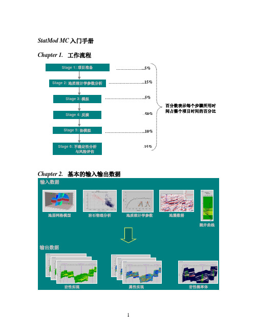
StatMod MC入门手册Chapter 1.工作流程输入数据输出数据岩性实现岩性概率体属性实现地质统计学参数岩石物理分析地层网格模型地震数据测井曲线………………...5%……………………..15%………………………..5%………………………..50%………………………..10%………………………….15%百分数表示每个步骤所用时间占整个项目时间的百分比Stage 4:反演Stage 2:地质统计学参数分析Stage 3:模拟Stage 5:协模拟Stage 1: 项目准备Stage 6: 不确定性分析与风险评估Chapter 3.详细操作步骤操作步骤以StatMod MC培训数据为例,共分十个练习来进行讲解。
第一步. 首先完成一个高质量的叠后CSSI反演(练习一内容)这一步的目的是为地质统计学提供一个好的研究基础, 这个“好”主要体现在:(1)好的井震标定, 目标区的相关值达到0.85以上;(2)好的叠后反演结果, 用来质控地质统计学模拟和反演结果, 是地质统计学反演结果横向预测准确度的参照物;(3)利用叠后反演结果进行砂体雕刻, 对目标区的岩性展布、比例有一个总体上正确的把握, 这些认识都是地质统计学的初始输入。
(说明:在提供的培训数据中已经为用户做了以上准备,用户可以从主界面中打开该培训数据所在工区/…../training_project/StatMod MC/training, 然后用Map View看工区底图,用Section View查看地震数据(../SEISMIC/full.mod)、叠后CSSI反演数据(../INVER_TRACE_PLUS/…)、地层网格模型数据(../SOLID/..)与层位数据(../SOLID_DIR/..),用Well Editor检查井震标定情况,井数据在(../WELLS/..)中)第二步. 测井数据准备(练习二内容)●●计算岩性曲线●●曲线重采样这一步将测井数据重采样至地质微层采样间隔,具体操作为:(1)JGW主界面→ Analysis→ Processing toolkit;(2)Input→ Data selection→ Data type:选Well, 点击Input file(s)右边List选择任意井(可以选多井),然后在弹出的界面Select logs中选择任意井曲线(可以多选),点击OK退出;(3)Parameters→ Resample log, 在弹出界面Processing toolkit中填写重采样间隔(注意s 与ms单位),点击OK退出;(4)Output→ Define process, 从Select from中选择Resample log, 点击››输入到右边的Process里面;(5)Output→ Generate, 在弹出的界面中填写输出路径和输出文件名,然后点击Generate,开始计算重采样的曲线.(说明:井数据的重采样数据在培训数据中已经为用户准备好了,在../WELLS/RESAMPLED/下面,并且井中也提供了相关曲线,如P-Impedance, Lithology, porosity等等)第三步. 地质统计学参数分析(练习三内容)这里说的地质统计学参数主要指三个参数:概率密度函数(probability density function, 简称pdf,描述某一属性在空间的概率分布情况)、云变换(描述两个属性之间的相关关系)、变差函数(描述某一属性随距离的变化,是距离的函数)。
DAEMON Tools使用操作说明

DAEMON Tools安装使用手册实验背景现在网上有很多游戏和软件都做成了ISO或者CCD等镜像格式。
有些游戏,比如大宇出品的轩辕剑、大富翁7等游戏,由于游戏盘是加密的,所以镜像文件只能做成mds格式的。
当你辛辛苦苦下载好这些软件和游戏,准备安装的时候,却发现文件图标都是未知类型的windows图标,无法打开,这下子要郁闷到极点了。
其实,只要你安装了DEAMON Tools,所有的镜像文件都能轻松搞定。
如果我们不想花钱买光盘去刻录某些系统盘,我们可以用DEAMON Tools将系统盘做成镜像格式,储存在硬盘中。
DEAMON Tools简介DEAMON Tools支持Win9x/Win2k/Winxp等系统,支持加密光盘,装完不需启动即可用。
是一个先进的模拟备份并且合并保护盘的软件,可以备份SafeDisc保护的软件,可以打开CUE,ISO and CCD 等这些虚拟光驱的镜像文件(以后将支持更多的格式)。
而且使用虚拟光驱还有很多其他的好处。
由于虚拟光驱和镜像文件都是对硬盘进行操作,因此可以减少真实的物理光驱的使用次数,延长光驱寿命。
同时,由于硬盘的读写速度要高于光驱很多,因此使用虚拟光驱,速度也大大提高,安装软件要比用真实光驱快4倍以上,游戏、软件安装的读盘停顿现象也会大大减少。
试验一DAEMON Tools的安装与配置实验目的掌握DAEMON Tools的安装过程及注意事项;熟悉DAEMON Tools的简单配置;熟悉DAEMON Tools各部分的功能实验内容软件版本:DAEMON Tools4.30步骤一安装一般从官方网站上当下来的是一个压缩包,解压后运行安装包,十分标准的安装过程。
只需点击“下一步”“完成”即可。
但其中有几点需要注意以下几点:1)图1.1中红色方框中的内容,安装时都会默认选择。
当鼠标移到每一项的上面时都会显示其代表的内容,可以根据自己的要求取舍;图1.1与Windows资源管?:是否新建一个“DEAMON ToolsLite”文件夹;浏览器:在浏览器上加载工具栏快捷地访问DEAMON官方网站,此项不要选;桌面快:是否在桌面设置一快捷启动项;开始菜单:是否在开始菜单中创建启动和卸载项,方便以后的操作;2)是否将图1.2中网站设置为你的浏览器的首页。
BD_FACSDiVa_软件操作手册
The first plots
At the top of the Worksheet Window you will find the "Tool Palette"
Clicking on the “DotPlot” icon activates the creation of DotPlots. Just click once on the worksheet to create a dotplot of “standard-size”. Dragging and holding the mouse creates a dotplot with the size of cour choice.
The user also controls which events are counted and stored: Storage Gate: Which events are recorded and saved Stopping Gate: Which cells are counted Events To Record: How many cells should be recorded (in the Stopping Gate)
• The software runs on a Windows2000 computer, Macintosh systems are no longer available
第二页,编辑于星期五:十二点 四十四分。
FACSDiVa Software
• The software uses a database server software to manage the flow cytometry data.
ASTAT工具使用简要说明
ASTAT工具使用简要说明1.安装:将文件夹“ASTAT”拷贝到电脑。
(免安装)2.连接:使用港迪提供的通讯电缆,9孔头连接电脑串口,9针头连接DARA(定子调压控制电路的小箱子)3.打开文件:连接好之后,运行“C:\ASTAT\PC program 10_052\English\Astat.exe”,点击“Open an existing project”,查找到所需要查看的参数文件。
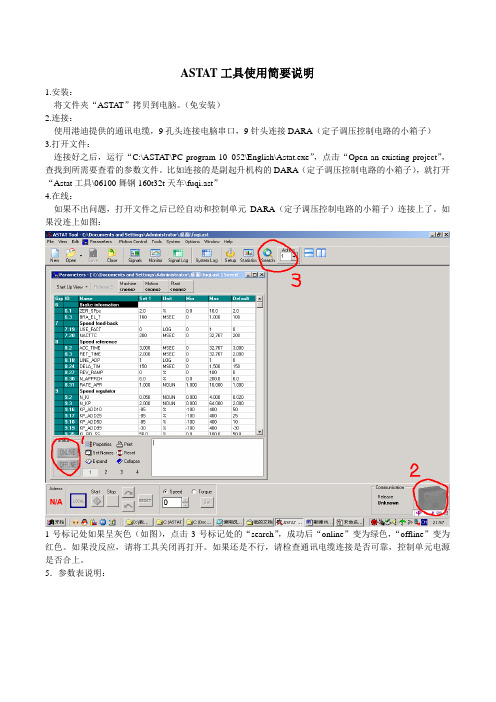
比如连接的是副起升机构的DARA(定子调压控制电路的小箱子),就打开“Astat工具\06100舞钢160t32t天车\fuqi.ast”4.在线:如果不出问题,打开文件之后已经自动和控制单元DARA(定子调压控制电路的小箱子)连接上了。
如果没连上如图:1号标记处如果呈灰色(如图),点击3号标记处的“search”,成功后“online”变为绿色,“offline”变为红色。
如果没反应,请将工具关闭再打开。
如果还是不行,请检查通讯电缆连接是否可靠,控制单元电源是否合上。
5.参数表说明:标记1:参数组号标记2:参数组名标记3:参数名标记4:参数值标记5:参数单位标记6:参数设定最小值标记7:参数设置最大值标记8:参数设置默认值标记9参数说明(英文的)参数10:参数号6.修改参数方法:先用鼠标正键选择需要修改的单元格如图:然后直接输入数值,屏幕上就会出现小对话框如图:7.修改完了所有参数之后就需要上传。
点击绿色的“online”按钮,弹出一个对话框,如图选择第一:将参数下载到定子调压;选择第二:将定子调压上的参数上载到电脑里,第三个是撤销操作。
下载完参数后就自动进入在线状态,这里可以在线修改参数。
需要保存在线修改的参数,需断开PC与定子调压的连接请点击红色按钮“offline”:出现对话框,点“yes”前保证当前机构的定子调压没有运行。
离线后,主控版显示“5C”才能再次动机构。
8.软件的详细使用介绍和说明请参考手册63页。
- 1、下载文档前请自行甄别文档内容的完整性,平台不提供额外的编辑、内容补充、找答案等附加服务。
- 2、"仅部分预览"的文档,不可在线预览部分如存在完整性等问题,可反馈申请退款(可完整预览的文档不适用该条件!)。
- 3、如文档侵犯您的权益,请联系客服反馈,我们会尽快为您处理(人工客服工作时间:9:00-18:30)。
StatMod只适用于三维工区。
主要算法:1. Sequential Gaussian Simulation (序贯高斯模拟) SGS2. Sequential Gaussian Collocated Co-simulation (序贯高斯配置协模拟) SGCCS3. Sequential Gaussian Co-simulation (序贯高斯协模拟) SGCS4. Sequential Indicator Simulation (序贯指示模拟,岩性模拟) SIS5. Lithology masks (遮挡岩性指示模拟)6. Sequential Indicator Simulation with a trend (带趋势的序贯指示模拟) SIS with trend7. Stochastic inversion (随机反演)一 、Sequential Gaussian Simulation (序贯高斯模拟) :----只用井数据作一种曲线的随机模拟例如对某一层(layer),用多井的孔隙度,进行 孔隙度的随机模拟。
一般需要15-20口井才会有效果分析:porosity first histogramfirst variogram(一) StatMod StatMod analysis …1、Input :(1) Variograms / transforms file … ( 键入文件名)simu.var(2) Trace gate … (3) Time / Depth mode … Time(4) Solid model … tdc1 ( 选EarthModel 的结果)(5) Layers … 选层(layer),例如:b.c 层(6) (作直方图分析)Well logs data …Model data …data …a) 选井文件:(选多个时域井文件)Log type : ( 选单一井曲线,如:porosity )出现 StatMod Transform 窗口Nr of intervals : 10 (直方图条数)出现直方图DoneUse automatic fitType Log – Ganssion (选任一种来拟By table 合分布函数)porosity_hist ( 存入simu.var )Assign current transform to selected layersOk Donee) Line width (置线条宽度)Title (写图名)Done(7)Data for variogram sampling and modeling --(作变异图分析)Primary data …Well log data ……a)选多个时域井文件选井曲线( porosity ),出现StatMod variogram 窗口Function注意:Indicator出现变异图)c) 可以扫描岩性的横向与纵向变化:(各向同性)(各向异性)(扫描储层的大致走向方向)Lateral Direction ( Azimuth )# of angles Angle Tolerance Bandwidth (m)Vertical Direction ( Dip ):Tolerance Bandwidth ( m )d) Anisotropy : Anisotropice) Okf)Func Type:可选 Gaussian或 Spherical来拟合数据点填写 sill 值与 x.y.z ( lag 值),可以反复调。
在 Gaussian simulation 中,Z 是主要的。
其中: Z: 纵向砂体的大致厚度X: 在走向方向上砂体的大致分布范围 (根据地质分析)Y: 在倾向方向上砂体的大致分布范围 (根据地质分析)操作步骤:填写 sill 值与 x.y.z ( lag 值)若不合适,点亮已有值(在最上边)修改 sill 值与 x.y.z ( lag 值)反复调整porosity_var (存入 saimu.var )DoneAssign current variogram to selected layersDone Ok!! 此时: 直方图 porosity_histsimu.var变异图 porosity_vari) Line width … 线条宽度Title 图头Done2、File Save & Exit(二) StatMod StatMod modeling …1、Input :(1) Simulation mode …Done(2) Time / Depth mode … Time(3) Solid model … 用EarthModel 的结果(4) Layers … 选层,例如:b.c 层,给采样间隔(5) Primary input data … Well log data …选多个时域井文件选单一井曲线 (如:porosity)(6) Variogram / transforms file … 选 simu.var(7) Trace gate …2、Edit:(1) Realization parameters … (实现参数)Nr of realization : 10 ----输出多个等概率的随机模拟结果(例如:10个)Output sample interval (s) : 0.001Perform kriging also (简单克里金)Use ordinary kriging (普通克里金)(2) Search parameters …Search radius (m) : 1000 ----扫描半径,要给大一些,大于井间距,否则不计算。
While krigingNumber of neighbors per octant : 4Use irregular search on primary dataWhile simulationNumber of neighbors per octant : 2Snap well to grid for fast performance(3) Transforms …选层(例如:b.c)与对应的直方图参数 porosity_hist(4) Variogram …层与对应的变异图参数 porosity_var(6) Super codes …Layer Super codeb bc c3、Output Generate …Run nowPrimary output Primary file name : ssm_bc_porosity_simu.modGenerate primary kriging error : ssm_bc_porosity_simu_error.mod并产生文件:(由于 Nr of realizations : 10 所以产生以下十个文件) ssm_bc_porosity_simu__01.modssm_bc_porosity_simu__02.modssm_bc_porosity_simu__03.mod 对孔隙度的10次随机 …… 模拟结果(等概率) ssm_bc_porosity_simu__10.mod4、File Save & Exit二、Sequential Gaussian Collocated Co-Simulation (序贯高斯配置协模拟): ------用井数据和阻抗体协同进行随机模拟,并与井匹配1、First ( porosity) -------- Histogram porosity_hist2、 First ( porosity) -------- Variogram porosity_var3、 Second (AI) --------- Histogram aitm_hist4、 两类数据的相关系数 (通过交会图分析)不需作互变异图(cross variogram),软件通过两类数据的相关系数实现协模拟。
(一) Statmod Analysis …第一类数据的直方图与变异图已分析过了,可以应用,不必再分析。
下边做第二类数据的分析:1、Input :(1) Variograms / transforms file … ( 选文件名)simu.var(2) Trace gate …(3) Data for histogram and transforms Model data …(a) aitm_ai.mod NoneDoneUse automatic fitaitm_hist Ok (存入simu.var)Assign current transform to selected layers Done(e) Done2、File Save & Exit(二)StatMod modeling …1、Input :(1) Simulation mode …(2) Time / Depth mode … Time(3) Solid model … tdc1(4) Layers … 选层与采样间隔(5) Primary input data … Well log data … 选井与曲线(porosity)(6) Secondary input data … Model data … aitm_ai.mod(7) Variogram / transforms file … simu.var(8) Trace gate …2、Edit :(1) Realization parameters …Nr of realization : 10Output sample interval (s) : 0.001Perform kriging alsoUse ordinary krigingUse cokriging second non-bias condition(2) Search parameters …GlobalSearch radius (m) : 10000While krigingNumber of neighbora per octant : 4Use irregular search on primary dataWhile simulationNumber of neighbors per octant : 2Snap well to grid for fast performance(3) Transforms …porosity_histaitm_hist(4) Variogram … porosity_var (5)Super codes … Layer Super code b bc c(7) Correlation coefficients …Layer Valueb 0.7 相关系数可通过交汇图大致给出c 0.73、Output Generate …Run nowPrimary outputPrimary file name : ssm_bc_SGCCS_first.modGenerate primary kriging error : ssm_bc_ SGCCS _first_error.mod并产生文件:(由于 Nr of realizations : 10 ,所以产生以下十个文件) ssm_bc_ SGCCS _first_01.modssm_bc_ SGCCS _first_02.mod 对孔隙度的配置协模拟结果ssm_bc_ SGCCS _first_03.mod……Secondary OutputGenerate secondary data : ssm_bc_ SGCCS _second.modGenerate primary kriging error : ssm_bc_ SGCCS _second_error.mod并产生以下十个文件 :ssm_bc_SGCCS_second_01.modssm_bc_SGCCS_second _02.mod 对阻抗的配置协模拟结果ssm_bc_SGCCS_second _03.mod……4、File Save & Exit三、Sequential Gaussian Co-Simulation : (序贯高斯协模拟)Transformsfirst : porosity (well)VariogramTransforms Cross Variogramsecond : aitm (cube)Variogram(一) SdatMod analysis …第一类数据的直方图与变异图和第二类数据的直方图均已分析完毕,下边需做第二类数据的变异图与两类数据的交会变异图。