哈工大导航原理大作业
哈工大GPS卫星导航实验报告4
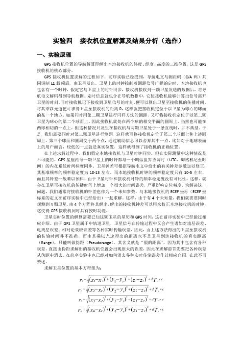
实验四接收机位置解算及结果分析(选作)一、实验原理GPS接收机位置的导航解算即解出本地接收机的纬度、经度、高度的三维位置,这是GPS 接收机的核心部分。
GPS接收机位置求解的过程如下:前序实验已经提到,导航电文与测距码(C/A码)共同调制L1载频后,由卫星发出。
卫星上的时钟控制着测距信号广播的定时。
本地接收机也包含有一个时钟,假定它与卫星上的时钟同步,接收机接收到一颗卫星发送的数据后,将导航电文解码得到导航数据。
定时信息就包含在导航数据中,它使接收机能够计算出信号离开卫星的时刻。
同时接收机记下接收到卫星信号的时刻,便可以算出卫星至接收机的传播时间。
将其乘以光速便可求得卫星至接收机的距离R,这样就把接收机定位于以卫星为球心的球面的某一个地方。
如果同时用第二颗卫星进行同样方法的测距,又可将接收机定位于以第二颗卫星为球心的第二个球面上。
因此接收机就处在两个球的相交平面的圆周上。
当然也可能在两球相切的一点上,但这种情况只发生在接收机与两颗卫星处于一条直线时,并不典型。
于是,我们需要同时对第三颗卫星进行测距,这样就可将接收机定位于第三个球面上和上述圆周上。
第三个球面和圆周交于两个点,通过辅助信息可以舍弃其中一点,比如对于地球表面上的用户而言,较低的一点就是真实位置,这样就得到了接收机的正确位置。
在上述求解过程中,我们假定本地接收机与卫星时钟同步,但在实际测量中这种情况是不可能的。
GPS星座内每一颗卫星上的时钟都与一个叫做世界协调时(UTC,即格林尼至时间)的内在系统时间标度同步。
卫星钟差可根据导航电文中给出的有关钟差参数加以修正,其基准频率的频率稳定度为10-13左右。
而本地接收机时钟的频率稳定度只有10-5左右,而且其钟差一般难以预料。
由于卫星时钟和接收机时钟的频率稳定度没有可比性,这样,就会在卫星至接收机的传播时间上增加一个很大的时间误差,严重影响定位精度。
为解决这一问题,我们通常将接收机的钟差也作为一个未知参数,与本地接收机的ECEF坐标(ECEF坐标系的定义在前序实验中已经给出)一起求解。
哈工大自动控制原理大作业
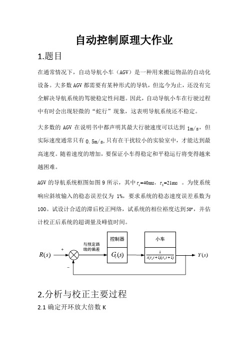
自动控制原理大作业1.题目在通常情况下,自动导航小车(AGV )是一种用来搬运物品的自动化设备。
大多数AGV 都需要有某种形式的导轨,但迄今为止,还没有完全解决导航系统的驾驶稳定性问题。
因此,自动导航小车在行驶过程中有时会出现轻微的“蛇行”现象,这表明导航系统还不稳定。
大多数的AGV 在说明书中都声明其最大行驶速度可以达到1m/s ,但实际速度通常只有0.5m/s ,只有在干扰较小的实验室中,才能达到最高速度。
随着速度的增加,要保证小车得稳定和平稳运行将变得越来越困难。
AGV 的导航系统框图如图9所示,其中12=40ms =21ms ττ, 。
为使系统响应斜坡输入的稳态误差仅为1%,要求系统的稳态速度误差系数为100。
试设计合适的滞后校正网络,试系统的相位裕度达到50 ,并估计校正后系统的超调量及峰值时间。
()R s ()Y s2.分析与校正主要过程2.1确定开环放大倍数K100)1021.0)(104.0(lim )(lim =++==s s s sK s sG K v (s →0) 解得K=100)1021.0)(104.0(100++=s s s G s 2.2分析未校正系统的频域特性根据Bode 图:穿越频率s rad c /2.49=ω相位裕度︒---=⨯-⨯--=99.18)2.49021.0(arctan )2.4904.0(arctan 9018011γ 未校正系统频率特性曲线由图可知实际穿越频率为s rad c /5.34=ω2.3根据相角裕度的要求选择校正后的穿越频率1c ω现在进行计算:︒︒︒--=+=---55550)021.0(arctan )04.0(arctan 901801111c c ωω则取s rad c /101=ω可满足要求2.4确定滞后校正网络的校正函数 由于11201~101c ωω)(=因此取s rad c /110111==ωω)(,则由Bode 图可以列出 40)1lg(20)1lg(40)110lg(2022+=+ωω 解得s rad /1.02=ω于是1.0=β 则滞后网络传递函数为1101)(++=s s s G c ,10=T 2.5验证已校正系统的相位裕度已校正系统的开环传递函数为:)110)(1021.0)(104.0()1(100)()(++++=s s s s s s G s G c 相位裕度︒----=-⨯-⨯-+-=2.51)100(arctan )10021.0(arctan )1004.0(arctan )10(arctan 901801111γ校正后的相位裕度大于50°,满足设计要求。
L1-导航原理(哈工大导航原理、惯性技术课件)讲解学习

陶瓷 壳体
球形 转子
球形电极 自转轴
钛离子泵
缺陷:结构复杂、昂贵
Lecture 1 -- Introduction
23
5.2 低成本、小型化
环形激光陀螺 (Ring laser gyro -- RLG) 1960s 早期开始研制, 1970s 后期进入实用
光纤陀螺 (Fiber Optical Gyro – FOG) 1970s 开始研制, 1980s 早期进入实用
15
4.2 历史: 陀螺罗经
陀螺仪被寄予希望, 但面临着自动寻北 的挑战
1908年, Anschutz (德国) 发明了陀螺罗经 (gyro compass)
1909年, Sperry (美国) 也独 立研制出陀螺罗经.
—— 陀螺罗经的出现标志着陀螺仪技术 的现代应用的发端
Lecture 1 -- Introduction
Lecture 1 -- Introduction
14
4.2 历史: 在航海的应用
磁罗盘 (Magnetic compass) 被用于早期的航海
19世纪后期,大量的木质 轮船被钢铁材质的轮船取代, 使磁罗盘的效能受到影响.
磁罗盘的使用在地球两极 附近受到限制 寻找替代的方向指示装置
Lecture 1 -- Introduction
Exam: Close book, close note Contact: 15204694662
Lecture 1 -- Introduction
28
此课件下载可自行编辑修改,仅供参考! 感谢您的支持,我们努力做得更好!谢谢
t
S
S0
Vdt
0
惯性导航的特点: 自主 (Autonomous, self-contained) 只依赖于对载体的惯性测量 (借助加速度计、陀螺仪) 连续稳定的输出
自01-哈工大机械原理大作业任务书-连杆机构参考模板
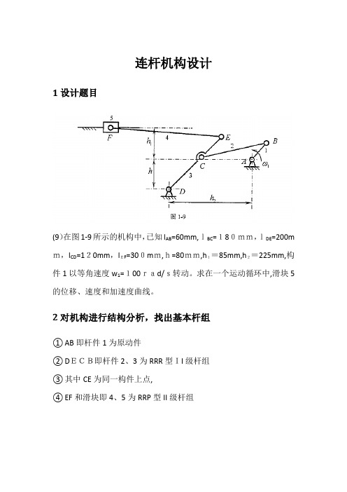
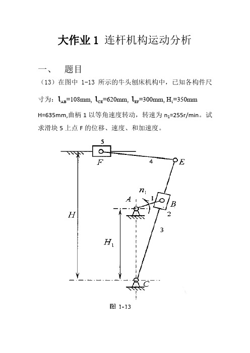
连杆机构设计1设计题目(9)在图1-9所示的机构中,已知l AB=60mm,lBC=180mm,lDE=200m m,l CD=120mm,lEF=300mm,h=80mm,h1=85mm,h2=225mm,构件1以等角速度w1=100rad/s转动。
求在一个运动循环中,滑块5的位移、速度和加速度曲线。
2对机构进行结构分析,找出基本杆组①AB即杆件1为原动件②DECB即杆件2、3为RRR型II级杆组③其中CE为同一构件上点,④EF和滑块即4、5为RRP型II级杆组3各基本杆组的运动分析数学模型② RRR 杆组运动分析的数学模型1.位置分析设两个构件长度1R ,2R 及外运动副1N ,2N 的位置已知,求两个构件的位置角1θ,2θ及内运动副3N 的位置。
选定坐标系及相应的标号如下图,构件的位置角i θ约定从响应构件的外运动副i N 引x 轴的方向线,按逆时针量取。
设外运动副1N ,2N 的位置坐标分别为1N (1x P ,1y P ),2N (2x P ,2y P ),则 12221212[( -)( -)]x x y y d P P P P =+ 222121cos ()/(2 )d R R R d α=++ 212 1arctan(( )/( )y y x x P P P P ϕ=-- 1θϕα=±内运动副3N 点坐标为:3111 cos x x P P R θ=+3111 sin y y P P R θ=+构件2K 的位置角:23232arctan[()/( )]y y x x P P P P θ=--位置分析过程中应注意两个问题:(1) 因为1N ,2N 的位置及杆长1R ,2R 都是给定的,这就可能出现d >12R R +或12d R R <-的情况。
在这两种情况下实际上不可能形成RRR 杆组,计算过程中应及时验算上述条件,如满足上述条件应中止运算并给出相应信息。
(2)在给定1N ,2N ,1R ,2R 的条件下,3N 可能有两个位置如上图中的3N 和3N ',相应的1θϕα=+和1θϕα'=-,我们称为杆组的两种工作状态。
哈工大惯性技术(导航原理)大作业讲解
Assignment of Inertial Technology 《惯性技术》作业Autumn 2015Assignment 1: 2-DOF response simulation A 2-DOF gyro is subjected to a sinusoidal torque with amplitude of 4 g.cmand frequency of 10 Hz along its outer ring axis. The angular moment of its rotor is 10000 g.cm/s , and the angular inertias in its equatorial plane are both 4 g.cm/s 2. Please simulate the response of the gyro within 1 second, and present whatever you can discover or confirm from the result.In this simulation, we are going to discuss the response of a 2-DOF gyro to sinusoidal torque input. According to the transfer function of the 2-DOF gyro, the outputs can be expressed as: 12222()()()()yx y x y x y J H s M s M s J J s H s J J s H α=-++ 12222()()()()x y x x y x y J H s M s M s J J s H s J J s H β=+++ The original system transfer function is a 2-input, 2-output coupling system. But the given input only exists one input, we can treat the system as 2 separate FIFO systemAs a consequence, we can establish the block diagram of the system in simulink in Fig 1.1. Substitute the parameters into the system and input, then we have the input signals as follow: 0,4sin(20)y ox M M t π==Then the inverse Laplace transform of the output equals the response of the gyro in timedomain as follows:02222000200222200()sin sin ()()()cos cos ()()ox a ox a x a x a ox ox a ox a a a a a M M t t t J J M M M t t t H H H ωαωωωωωωωωωβωωωωωωωω=-+--=+---Fig 1.1 The block diagram of the system in simulinkAnd the simulation results in time domain within 1 second are shown in the follwing pictures. Fig1.2 is the the output of outer ring ()tα. Fig1.3 is the output of inner ring ()tβ. Fig1.4 is the trajectory of 2-DOF gyro’s response to sinusoidal input. As we can see from the Fig1.3,there are obvious sawtooth wave in the output of the inner ring. It’s a unexpected phenomenon in my original theoretical analysis.Fig1.2 The output of inner ring ()tβFig 1.3 The output of outer ring ()tαI believe the sawtooth wave is caused by the nutation. For the frequency of the nutation isobtained as100002500/3974eHrad s HzJω===≈, which is far higher than the frequencyof the applied sinusoidal torque , namelyaωω.Fig 1.4 Trajectory of 2-DOF gyro’s response to sinusoidal input The trajectory of 2-DOF gyro’s response to sinusoidal input are shown in Fig1.4. As we can see, it’s coupling of X and Y channel scope output. The overall shape is an ellipse, which is not perfect for there are so many sawteeth on the top of it.Note that the major axis of ellipse is in the direction of the forced procession, amplitude of which isoxMHω, whereas the minor axis is in the direction of the torsion spring effects, with amplitude oxaMHω.The nutation components are much smaller than that of the forced vibration, which can be eliminated to get the clear static response.2200222()sin sin()cos(1cos)()ox oxa ax aox ox oxa aa a a aM Mt t tJ HM M Mt t tH H Hαωωωωωωβωωωωωωω≈≈-≈-=--To prove it, we eliminate the effects of the nutation namely the quadratic term in the denominator and get Fig 1.5, which is a perfect ellipse. We can conclude that when input to the 2-DOF gyro is sinusoidal torque, the gyro will do an ellipse conical pendulum as a static response, including procession and the torsion spring effects, together with a high-frequency vibration as the dynamic response.Fig 1.5 Trajectory of the gyro’s response without nutationAssignment 2: Single-axis INS simulation2.1 description of the problemA magnetic levitation train is being tested along a track running north-south. It first accelerates and then cruises at a constant speed. Onboard is a single-axis platform INS, working in the way described by the courseware of Unit 5: Basic problems of INS. The motion information and Earth parameters are shown in table 2-1, and the possible error sources are shown in Table2-2.Fig2.1 The sketch map of the single-axis INS problemYou are asked to simulate the operation of the INS within 10,000 seconds, and investigate, first one by one and then altogether, the impact of these error sources on the performance of the INS.The block diagram in the courseware might be of some help. However, there lurks an inconspicuous error, which you have to correct before you can obtain reasonable results.There are one core relevant formula, to get the specific form of its solution, we should substitute the unknown parameters.(1)()c N ay A K y ga=∆++-Firstly, the input signal is accelerometer of the platform, and the velocity of the platform is the integration of the acceleration./py y ydty Rω=+=-⎰The acceleration along Yp may contains two parts:cos gsin gypf y yααα=-≈-When accelerometer errors are concerned, the output of accelerometer will be:(1)N a yp Na K f A=++When gyro errors concerned:'(1)p g pKωωε=++Only αis unknown:[(1)]tg pttptK dtdtααωεϕϕω=+++-∆∆=⎰⎰And the reference block diagram and simulink block diagram are as follows in Fig2.2, Fig2.3. There is a small fault in the reference block, which is that the sign of the marked add operation should be positive instead of negative.The results of the simulation are shown in Fig 2.4 to Fig 2.13.Fig2.2 The reference block diagram in the courseware(unrectified)Fig2.3 The simulink block diagram for Assignment 22.2 results and analysis of the problemFig.2.4 real acceleration,velocity and displacement output without error sourcesKFig2.5 position bias when only accelerometer scale factor error exists0.0001aFig2.6 position bias output when only gyro scale factor error exists 0.0001g K =Fig2.7 position bias when only acceleromete bias error exists 20.0002/N A m s ∆=Fig2.8 position bias output when only initial velocity error exists 200.01/y m s ∆=Fig2.9 position bias output when only initial position error exists 010y m ∆=Fig2.10 position bias output bias when only gyro bias errorexists 0.000000024240.00681/3/h rad s ε=︒=Fig2.11 position bias output when only initial platform misalignment angle exists0.000012120''345radα==Fig2.12 output considering all the error sourcesFig2.13 position bias output considering all error sourcesAs we can see in the above simulation results, if there is no error we can navigate the train ’s motion correctly, which comes from north to the south as shown in Fig2.4, beginning with an constant acceleration within 60 seconds then cruises at a constant speed, approximately 65 m/s. However, the situation will change a lot when different errors put into the simulation. The initial position error 010y m ∆= effects least as Fig.2.8, for this error doesn ’t enter into the closed loop and it won ’t influence the iterative process. The position bias is constant and can be negligible.In the second case, when the accelerometer scale factor error exists, 0.0001a K =, as shown in Fig2.5, the result are stable and almost accurate, the position bias is a sinusoidal output.So it is with the accelerometer bias error situation, 20.0002/N A m s ∆=, in Fig2.7, the initialvelocity error, 200.01/y m s ∆= in Fig2.9, and the initial platform misalignment angle,05''α=, in Fig2.11. However, the influence degrees of the different factors are not in the samemagnitude. The accelerometer scale factor influences the least with magnitude of 5, then the initial velocity larger magnitude of 8, and the accelerometer bias magnitude of 25. The influence of the initial platform misalignment angle is much more significant with a magnitude of 150. All the navigation bias in the second kind case is sinusoidal, which means they ’re limited and negligible as time passes by.In the third case, such as the gyro scale factor error situation, 0.0001g K =, in Fig2.6, and the gyro bias error,0.01/h ε=︒, results in Fig2.10, effects the most significant, the trajectory of the navigation disvergence accumulated as time goes. The position bias is a combination of sinusoidal signal and ramp signal. They also show that the longitudinal and distance errors resulted from gyro drifts are not convergent in time. It means the errors in the gyroscope do most harm to our navigation. And due to the significant influence of the gyro bias errors and the gyroscope scale factor error, results considering all the error sources disverge, and the navigationposition of the motion will be away from the real motion after a enough long time, as shown in Fig2.10. The gyro bias error is the most significant effect factor of all errors. By the time of 10000s, it has reaches 1600m, and it’s nearly the quantity of the position bias considering all error sources. Through contrasting all the results, We can conclude that the gyro bias error is the main component of the whole position bias.Impression of the Whole simulation experimentThrough contrasting all the results, We can conclude that the gyro bias error is the main component of the whole position bias, and the the gyro bias or the drift error do most harm to our navigation. So it is a must for us to weaken or eliminate it anyway. In spite of all the disadvantages discussed above, the INS still shows us a relatively accurate results of single-axis navigation.Assignment 3: SINS simulation3.1 Task descriptionA missile equipped with SINS is initially at the position of 46o NL and 123 o EL, stationary on a launch pad. Three gyros, GX, GY, GZ, and three accelerometers, AX, AY, AZ, are installed along the axes Xb, Yb, Zb of its body frame respectively.Case 1: stationary testThe body frame of the missile initially coincides with the geographical frame, as shown in the figure, with its pitching axis Xb pointing to the east, rolling axis Yb to the north, and azimuth axis Zb upward. Then the body of the missile is made to rotate in 3 steps:(1) -22o around Xb(2) 78o around Yb(3) –16o around ZbFig 3.1 Introduction to assignment 3After that, the body of the missile stops rotating. You are required to compute the final outputs of the three accelerometers on the missile, using quaternion and ignoring the device errors. It is known that the magnitude of gravity acceleration is g = 9.8m/s2.Case 2: flight tes tInitially, the missile is stationary on the launch pad, 400m above the sea level. Its rolling axis is vertical up,and its pitching axis is to the east. Then the missile is fired up. The outputs of the gyros and accelerometers are both pulse numbers. Each gyro pulse is an angular increment of 0.01arc-sec, and each accelerometer pulse is 1e-7g, with g =9.8m/s2. The gyro output frequency is 200Hz, and the accelerometer’s is 10Hz. The outputs of the gyros and accelerometers within 1315s are stored in a MA TLAB data file named imu.mat, containing matrices gm of 263000× 3 and am of 13150× 3 respectively. The format of the data is as shown in the tables, with 10 rows of each matrix selected. Each row represents the outputs of the type of sensors at each sampling time. The Earth can be seen as an ideal sphere, with radius 6371.00km and spinning rate 7.292× 10⁻⁵ rad/s, The errors of the sensors are ignored, so is the effect of height on the magnitude of gravity. The outputs of the gyros are to be integrated every 0.005s. The rotation of the geographical frame is to be updated every 0.1s, so are the velocities and positions of the missile.You are required to:(1) compute the final attitude quaternion, longitude, latitude, height, and east, north, vertical velocities of the missile.(2) compute the total horizontal distance traveled by the missile.(3) draw the latitude-versus-longitude trajectory of the missile, with horizontal longitude axis.(4) draw the curve of the height of the missile, with horizontal time axis.Fig 3.2 simplified navigation algorithm for SINS 3.2Procedure code3.2.1 Sub function code:quaternion multiply code:function [q1]=quml(q1,q2);lm=q1(1);p1=q1(2);p2=q1(3);p3=q1(4);q1=[lm -p1 -p2 -p3;p1 lm -p3 p2;p2 p3 lm -p1;p3 -p2 p1 lm]*q2;endquaternion inversion code:function [qni] =qinv(q)q(1)=q(1);q(2)=-q(2);q(3)=-q(3);q(4)=-q(4);qni=q;end3.2.2case1 DCM algorithm:function ans11cz=[cos(-22/180*pi) sin(-22/180*pi) 0 ;-sin(-22/180*pi) cos(-22/180*pi) 0;0 0 1]; %The third rotation DCMcx=[1 0 0 ;0 cos(78/180*pi) sin(78/180*pi);0 -sin(78/180*pi) cos(78/180*pi)]; %The first rotation DCMcy=[cos(-16/180*pi) 0 -sin(-16/180*pi);0 1 0;sin(-16/180*pi) 0 cos(-16/180*pi)]; %The second rotation DCM A=cz*cy*cx*[0;0;-9.8]end3.2.3case1 quaternion algorithm:function ans12g=[0;0;0;-9.8];q1=[cos(-11/180*pi);sin(-11/180*pi);0;0]; %The first rotation quaternionq2=[cos(39/180*pi);0;sin(39/180*pi);0]; %The second rotation quaternionq3=[cos(-8/180*pi);0;0;-sin(-8/180*pi)]; %The third rotation quaternionr=quml(q1,q2); %call the quaternion multiplication subfunction q=quml(r,q3);P1=[q(1) q(2) q(3) q(4);-q(2) q(1) q(4) -q(3);-q(3) -q(4) q(1) q(2);-q(4) q(3) -q(2) q(1)];P2=[q(1) -q(2) -q(3) -q(4);q(2) q(1) q(4) -q(3);q(3) -q(4) q(1) q(2);q(4) q(3) -q(2) q(1)];P=P1*P2;gn=P*g;gn=gn(2:4)end3.2.4 case2 SINS quaternion algorithm code:function ans2clc;clear;%parameters initializing:T=0.005;K=13150;R=6371000; %radius of earthwE=7.292*10^(-5); %spinning rate of earthQ=zeros(4, 263001) ;%quaternion matrix initializinglongitude=zeros(1,13151);latitude=zeros(1,13151);H=zeros(1,13151); %altitude matrixQ(:,1)=[cos(45/180*pi);-sin(45/180*pi);0;0]; % initial quaternion longitude(1)=123; %initial longitudelatitude(1)=46; % initial latitudeH(1)=400; %initial altitudelength=0;g=9.8;vE = zeros(1,13151); %eastern velocityvN = zeros(1,13151); %northern velocityvH = zeros(1,13151); %upward velocityvE(1)=0;vN(1)=0;vH(1)=0;load imu.mat %data loading%main calculation sectionfor N=1:Kq1=zeros(4,11);q1(:,1)=Q(:,N);for n=1:20 % Attitude iteration wx=0.01/(3600*180)*pi*gm((N-1)*10+n,1); % Angle incrementwy=0.01/(3600*180)*pi*gm((N-1)*10+n,2);wz=0.01/(3600*180)*pi*gm((N-1)*10+n,3);w=[wx,wy,wz]';normw=norm(w); % Norm calculationW=[0,-w(1),-w(2),-w(3);w(1),0,w(3),-w(2);w(2),-w(3),0,w(1);w(3),w(2),-w(1),0];I=eye(4);S=1/2-normw^2/48;C=1-normw^2/8;q1(:,n+1)=(C*I+S*W)*q1(:,n);Q(:,N+1)=q1(:,n+1);endWE=-vN(N)/R; % rotational angular velocity component of a geographic coordinate systemWN=vE(N)/R+wE*cos(latitude(N)/180*pi);WH=vE(N)/R*tan(latitude(N)/180*pi)+wE*sin(latitude(N)/180*pi);attitude=[WE,WN,WH]'*T; %correction of the quaternion by updating the rotation of geographic coordinatenormattitude=norm(attitude);e=attitude/normattitude;QG=[cos(normattitude/2);sin(normattitude/2)*e];Q(:,N+1)=quml(qinv(QG),Q(:,N+1));fx=1e-7*9.8*am(N,1); %specific force measured by accelerometerfy=1e-7*9.8*am(N,2);fz=1e-7*9.8*am(N,3);Fb=[fx fy fz]';F=quml(Q(:,N+1),quml([0;Fb],qinv(Q(:,N+1)))); %The specific force is decomposed into geographic coordinate system.FE(N)=F(2);FN(N)=F(3);FU(N)=F(4);%calculate the velocity of the vehicle:VED(N)=FE(N)+vE(N)*vN(N)/R*tan(latitude(N)/180*pi)-(vE(N)/R+2*wE*cos(latitude(N)/ 180*pi))*vH(N)+2*vN(N)*wE*sin(latitude(N)/180*pi);VND(N)=FN(N)-2*vE(N)*wE*sin(latitude(N)/180*pi)-vE(N)*vE(N)/R*tan(latitude(N)/180 *pi)-vN(N)*vH(N)/R;VUD(N)=FU(N)+2*vE(N)*wE*cos(latitude(N)/180*pi)+(vE(N)^2+vN(N)^2)/R-g;%integration and get the relative velocity of vehicle:vE(N+1)=VED(N)*T+vE(N);vN(N+1)=VND(N)*T+vN(N);vH(N+1)=VUD(N)*T+vH(N);% integration and get the position of vehicle:longitude(N+1)=vE(N)/(R*cos(latitude(N)/180*pi))*T/pi*180+longitude(N);latitude(N+1)=vN(N)/R*T/pi*180+latitude(N);H(N+1)=vH(N)*T+H(N);length=sqrt((vE(N))^2+(vN(N))^2)+length;endfigure(1) %picture the longitude-latitude curve of the motion within 1315 secondstitle(' longitude-latitude ');hold ongrid onplot(longitude,latitude);figure(2) % picture the altitude curve of the motion within 1315 secondstitle('altitude');hold ongrid onplot(0:13150,H);3.3Simulation outputs and results analysisIn case 1, the DCM algorithm and quaternion results are the same as follow:A =7.53165.9788-1.8892And the results suggest the solution of DCM and quaternion is equivalence in this problem.In case 2, the latitude-versus-longitude trajectory of the missile(with horizontal longitude axis) and the altitude curve of the missile are shown as follows in Fig 3.3 and Fig 3.4.Fig3.3 the latitude-versus-longitude trajectory of the missile(with horizontal longitude axis)Fig3.4the altitude curve of the missileImpression of the Assignment 3In this assignment, we simulate the missile navigation situation in a real problem, as the problem we have done before. I did this based on my own original code, but to my surprise, it’s harder than I have expected. For the detailed thoughts for my program I have forgotten. I have to recheck the code line by line, But I am still troubled in correcting the initial parameters for many times. It has taught me a lesson, which is never to be egotistical for your ability to memory and the work you have done or understood.。
卫星定位导航原理知到章节答案智慧树2023年哈尔滨工业大学

卫星定位导航原理知到章节测试答案智慧树2023年最新哈尔滨工业大学第一章测试1.北斗三代系统的组成是()。
参考答案:24 MEO+3 GEO+3 IGSO2.下列不属于GPS的功能的是()参考答案:短报文通信3.()导航系统覆盖范围在2000km~3000km之间。
参考答案:远程导航系统4.对于GPS系统,地面观测者相同方位每天提前()见到同一颗GPS卫星。
参考答案:4min5.北斗系统包含哪些部分()。
参考答案:其余都是6.下图星座是()参考答案:北斗7.导航系统的技术指标主要有()。
参考答案:定位速率;系统可靠性;覆盖范围;定位精度8.下列属于GPS的功能的是()参考答案:授时;测速;定位导航9.子午系统的地面控制部分包括()。
参考答案:控制中心;注入站;跟踪站10.子午星系统有8颗卫星。
()参考答案:错11.北斗二代系统是被动定位系统。
()参考答案:对12.以下星座不可以达到全球全天候不间断覆盖的效果。
()参考答案:错第二章测试1.开普勒方程是描述偏近点角和()的关系。
参考答案:平近点角2.由于地球自转轴收到地球内部质量不均匀影响,地极点在地球表面上位置随时间而变化的现象称为()。
参考答案:极移现象3.确定卫星在轨道上的顺势为之的开普勒轨道参数是()。
参考答案:真近点角4.关于以下电文帧结构,说法不正确的是()。
参考答案:该电文帧为北斗电文帧5.下式中,旋转哪个参量是使得轨道平面与赤道平面相重合()。
参考答案:6.开普勒第三定律与()有关。
参考答案:轨道长半轴;卫星运行周期7.以下关于GPS卫星导航电文的描述正确的是()。
参考答案:基本单位长度为1500bit;一个主帧包括5个子帧8.星历信息中不包括()参考答案:卫星时钟校正量;卫星识别号和健康状态;全部卫星的粗略星历9.协议天球坐标系需要扣除()参考答案:章动现象;岁差现象10.协议地球坐标系最终要转化为协议天球坐标系。
()参考答案:错11.如果考虑接收机钟差,4颗星即可定位。
导航原理 大作业 哈工大

2. 程序设计说明及代码
2.1 仿真需要的两个子程序 (1)四元数求逆子函数 %四元数求逆函数 function [ qni ] = qiuni( q ) q(1)=q(1); q(2)=-q(2); q(3)=-q(3); q(4)=-q(4); qni=q; end (2)四元数相乘子程序 %四元数相乘计算函数 function [q]=quml(q1,q2); lm=q1(1);p1=q1(2);p2=q1(3);p3=q1(4); q=[lm -p1 -p2 -p3;p1 lm -p3 p2;p2 p3 lm -p1;p3 -p2 p1 lm]*q2; end 2.2 第一种情形:正对导弹进行地面静态测试(导弹质心相对地面静止) (1)用方向余弦矩阵计算,MATLAB 程序如下: function dcm g0=[0;0;9.8];%重力加速度在地里坐标系中的分量表示 wx=15/180*pi; wy=20/180*pi; wz=-10/180*pi; w=sqrt(wx^2+wy^2+wz^2); %四阶近似 I=eye(3); S=1-w^2/6; C=1/2-w^2/24; W=[0,-wz,wy;wz,0,-wx;-wy,wx,0]; c=I+S*W+C*W^2;%载体坐标系到初始坐标系的方向余弦阵 c=inv(c)%初始坐标系到载体坐标系的方向余弦阵 g=c*g0%重力加速度在载体坐标系中的分量 end 在MATLAB命令窗口输入dcm,即得到如下结果: c = 0.9253 0.2129 0.3139 -0.1233 0.9515 -0.2821 -0.3587 0.2223 0.9067
g = -3.5160 2.1791 8.8842 2.3 第二种情形:导弹正在飞行中 MATLAB 程序如下: %主程序
导航原理实验报告

导航原理实验报告院系:班级:学号:姓名:成绩:指导教师签字:批改日期:年月日哈尔滨工业大学航天学院控制科学实验室实验1 二自由度陀螺仪基本特性验证实验一、实验目的1.了解机械陀螺仪的结构特点;2.对比验证没有通电和通电后的二自由度陀螺仪基本特性表观; 3.深化课堂讲授的有关二自由度陀螺仪基本特性的内容。
二、思考与分析1. 定轴性(1) 设陀螺仪的动量矩为H ,作用在陀螺仪上的干扰力矩为M d ,陀螺仪漂移角速度为ωd ,写出关系式说明动量矩H 越大,陀螺漂移越小,陀螺仪的定轴性(即稳定性)越高.答案:d d H M ω=⨯u u u r u u r u u r/sin d dH M θω= 干扰力矩M d 一定时,动量矩H 越大,陀螺仪漂移角速度为ωd 越小,陀螺漂移越小,陀螺仪的定轴性(即稳定性)越高.(2) 在陀螺仪原理及其机电结构方而简要蜕明如何提高H 的量值?答案:H J =Ωu u r u r 由公式2AJ dm r =⎰⎰⎰可知提高H 的量值有四种途径:1. 陀螺转子采用密度大的材料,其质量提高了,转动惯量也就提高了。
2. 改变质量分布特性。
在质量相同的情况下,若质量分布的半径距质心越远,H 越大。
因此将陀螺转子的有效质量外移,如动力谐陀螺将转子设计成环状。
即在陀螺电机定子环中,可做成质量集中分布在环外边缘的环形结构,切边缘部分材质密度大,可提高转动惯量。
3. 增大r,可有效提高转动惯量。
4. 另外可通过采用外转子电机来改变电机质量分布,增大r 。
改变电机定转子结构:采用外转子,内定子结构的转子电机。
4. 增加陀螺转子的旋转速度。
2/602(1)/n s f p ωππ==- ,60(1)/n f s p =-提高电压周波频率 f ↑——〉n ↑——H ↑ f=400Hz适当减少极对数 ,如取p=1适当减少转差率s ,可通过减少转子支承轴承摩擦来实现2.进动性(1) 在外框架施加一沿x 轴正方向作用力矩时,画出动量矩H 的进动方向及矢量M ,ω,H 的关系坐标图。
哈工大卫星定位导航原理实验报告

卫星定位导航原理实验专业:班级:学号:姓名:日期:实验一实时卫星位置解算及结果分析一、实验原理实时卫星位置解算在整个GPS接收机导航解算过程中占有重要的位置。
卫星位置的解算是接收机导航解算(即解出本地接收机的纬度、经度、高度的三维位置)的基础。
需要同时解算出至少四颗卫星的实时位置,才能最终确定接收机的三维位置。
对某一颗卫星进行实时位置的解算需要已知这颗卫星的星历和GPS时间。
而星历和GPS时间包含在速率为50比特/秒的导航电文中。
导航电文与测距码(C/A码)共同调制L1载频后,由卫星发出。
本地接收机相关接收到卫星发送的数据后,将导航电文解码得到导航数据。
后续导航解算单元根据导航数据中提供的相应参数进行卫星位置解算、各种实时误差的消除、本地接收机位置解算以及定位精度因子(DOP)的计算等工作。
关于各种实时误差的消除、本地接收机位置解算以及定位精度因子(DOP)的计算将在后续实验中陆续接触,这里不再赘述。
卫星的额定轨道周期是半个恒星日,或者说11小时58分钟2.05秒;各轨道接近于圆形,轨道半径(即从地球质心到卫星的额定距离)大约为26560km。
由此可得卫星的平均角速度ω和平均的切向速度v s为:ω=2π/(11*3600+58*60+2.05)≈0.0001458rad/s (1.1)v s=rs*ω≈26560km*0.0001458≈3874m/s (1.2) 因此,卫星是在高速运动中的,根据GPS时间的不同以及卫星星历的不同(每颗卫星的星历两小时更新一次)可以解算出卫星的实时位置。
本实验同时给出了根据当前星历推算出的卫星在11小时58分钟后的预测位置,以此来验证卫星的额定轨道周期。
本实验另一个重要的实验内容是对卫星进行相隔时间为1s的多点测量(本实验给出了三点),根据多个点的测量值,可以估计Doppler频移。
由于卫星与接收机有相对的径向运动,因此会产生Doppler效应,而出现频率偏移。
哈工大惯性技术(导航原理)大作业

Assignment ofInertial Technology《惯性技术》作业My Chinese NameMy Student ID 15S004001Autumn 2015Assignment 1: 2-DOF response simulationA 2-DOF gyro is subjected to a sinusoidal torque with amplitude of 4 g.cm and frequency of 10 Hz along its outer ring axis. The angular moment of its rotor is 10000 g.cm/s , and the angular inertias in its equatorial plane are both 4 g.cm/s 2. Please simulate the response of the gyro within 1 second, and present whatever you can discover or confirm from the result.In this simulation, we are going to discuss the response of a 2-DOF gyro to sinusoidal torque input. According to the transfer function of the 2-DOF gyro, the outputs can be expressed as:12222()()()()yx y x y x y J Hs M s M s J J s H s J J s H α=-++12222()()()()x yx x y x y J Hs M s M s J J s H s J J s H β=+++ The original system transfer function is a 2-input, 2-output coupling system. But the given input only exists one input, we can treat the system as 2 separate FIFO systemAs a consequence, we can establish the block diagram of the system in simulink in Fig 1.1. Substitute the parameters into the system and input, then we have the input signals as follow: 0,4sin(20)y ox M M t π==Then the inverse Laplace transform of the output equals the response of the gyro in timedomain as follows:0222200020222200()sin sin ()()()cos cos ()()ox a oxa x a x a ox ox a ox a a a a a M M t t t J J M M M t t t H H H ωαωωωωωωωωωβωωωωωωωω=-+--=+---Fig 1.1 The block diagram of the system in simulinkAnd the simulation results in time domain within 1 second are shown in the follwing pictures. Fig1.2 is the the output of outer ring ()t α. Fig1.3 is the output of inner ring ()t β. Fig1.4 is the trajectory of 2-DOF gyro ’s response to sinusoidal input. As we can see from the Fig1.3,there are obvious sawtooth wave in the output of the inner ring. It ’s a unexpected phenomenon in my original theoretical analysis.Fig1.2 The output of inner ring ()t βFig 1.3 The output of outer ring ()t αI believe the sawtooth wave is caused by the nutation. For the frequency of the nutation is obtained as010*******/3974e H rad s Hz J ω===≈, which is far higher than the frequencyof the applied sinusoidal torque , namely0a ωω .Fig 1.4 Trajectory of 2-DOF gyro ’s response to sinusoidal inputThe trajectory of 2-DOF gyro ’s response to sinusoidal input are shown in Fig1.4. As we can see, it ’s coupling of X and Y channel scope output. The overall shape is an ellipse, which is not perfect for there are so many sawteeth on the top of it.Note that the major axis of ellipse is in the direction of the forced procession, amplitude of which is 0ox M H ω, whereas the minor axis is in the direction of the torsion spring effects,with amplitude ox aM H ω.The nutation components are much smaller than that of the forced vibration, which can be eliminated to get the clear static response.22002220()sin sin ()cos (1cos )()ox oxaa x a ox ox oxa a a a a aM M t t t J H M M M t t t H H H αωωωωωωβωωωωωωω≈≈-≈-=--To prove it, we eliminate the effects of the nutation namely the quadratic term in the denominator and get Fig 1.5, which is a perfect ellipse. We can conclude that when input to the 2-DOF gyro is sinusoidal torque, the gyro will do an ellipse conical pendulum as a static response, including procession and the torsion spring effects, together with a high-frequency vibration as the dynamic response.Fig 1.5 Trajectory of the gyro’s response without nutationAssignment 2: Single-axis INS simulation2.1 description of the problemA magnetic levitation train is being tested along a track running north-south. It first accelerates and then cruises at a constant speed. Onboard is a single-axis platform INS, working in the way described by the courseware of Unit 5: Basic problems of INS. The motion informationand Earth parameters are shown in table 2-1, and the possible error sources are shown in Table2-2.Fig2.1 The sketch map of the single-axis INS problemYou are asked to simulate the operation of the INS within 10,000 seconds, and investigate,first one by one and then altogether, the impact of these error sources on the performance of theINS.The block diagram in the courseware might be of some help. However, there lurks aninconspicuous error, which you have to correct before you can obtain reasonable results.There are one core relevant formula, to get the specific form of its solution, we should substitute the unknown parameters.(1)()c N a y A K yga =∆++-Firstly, the input signal is accelerometer of the platform, and the velocity of the platform is the integration of the acceleration.0/p y y ydt yR ω=+=-⎰The acceleration along Yp may contains two parts:cos gsin g yp f y yααα=-≈- When accelerometer errors are concerned, the output of accelerometer will be:(1)N a yp N a K f A =++When gyro errors concerned:'(1)p g p K ωωε=++Onlyαis unknown:000[(1)]tg p t tp t K dt dtααωεϕϕω=+++-∆∆=⎰⎰And the reference block diagram and simulink block diagram are as follows in Fig2.2, Fig2.3. There is a small fault in the reference block, which is that the sign of the marked add operation should be positive instead of negative.The results of the simulation are shown in Fig 2.4 to Fig 2.13.Fig2.2 The reference block diagram in the courseware(unrectified)Fig2.3 The simulink block diagram for Assignment 22.2 results and analysis of the problemFig.2.4 real acceleration,velocity and displacement output without error sourcesKFig2.5 position bias when only accelerometer scale factor error exists0.0001aFig2.6 position bias output when only gyro scale factor error exists 0.0001g K =Fig2.7 position bias when only acceleromete bias error exists 20.0002/N A m s ∆=Fig2.8 position bias output when only initial velocity error exists 200.01/ym s ∆=Fig2.9 position bias output when only initial position error exists 010y m ∆=Fig2.10 position bias output bias when only gyro bias error exists 0.000000024240.00681/3/h rad s ε=︒=Fig2.11 position bias output when only initial platform misalignment angle exists0.000012120''345radα==Fig2.12 output considering all the error sourcesFig2.13 position bias output considering all error sourcesAs we can see in the above simulation results, if there is no error we can navigate the train ’s motion correctly, which comes from north to the south as shown in Fig2.4, beginning with an constant acceleration within 60 seconds then cruises at a constant speed, approximately 65 m/s. However, the situation will change a lot when different errors put into the simulation. The initial position error 010y m ∆= effects least as Fig.2.8, for this error doesn ’t enter into the closed loop and it won ’t influence the iterative process. The position bias is constant and can be negligible.In the second case, when the accelerometer scale factor error exists, 0.0001a K =, as shown in Fig2.5, the result are stable and almost accurate, the position bias is a sinusoidal output. So it is with the accelerometer bias error situation, 20.0002/N A m s ∆=, in Fig2.7, the initialvelocity error, 200.01/ym s ∆= in Fig2.9, and the initial platform misalignment angle, 05''α=, in Fig2.11. However, the influence degrees of the different factors are not in the samemagnitude. The accelerometer scale factor influences the least with magnitude of 5, then the initial velocity larger magnitude of 8, and the accelerometer bias magnitude of 25. The influence of the initial platform misalignment angle is much more significant with a magnitude of 150. All the navigation bias in the second kind case is sinusoidal, which means they ’re limited and negligible as time passes by.In the third case, such as the gyro scale factor error situation, 0.0001g K =, in Fig2.6, and the gyro bias error,0.01/h ε=︒, results in Fig2.10, effects the most significant, the trajectory of the navigation disvergence accumulated as time goes. The position bias is a combination of sinusoidal signal and ramp signal. They also show that the longitudinal and distance errors resulted from gyro drifts are not convergent in time. It means the errors in the gyroscope do most harm to our navigation. And due to the significant influence of the gyro bias errors and the gyroscope scale factor error, results considering all the error sources disverge, and the navigationposition of the motion will be away from the real motion after a enough long time, as shown in Fig2.10. The gyro bias error is the most significant effect factor of all errors. By the time of 10000s, it has reaches 1600m, and it’s nearly the quantity of the position bias considering all error sources. Through contrasting all the results, We can conclude that the gyro bias error is the main component of the whole position bias.Impression of the Whole simulation experimentThrough contrasting all the results, We can conclude that the gyro bias error is the main component of the whole position bias, and the the gyro bias or the drift error do most harm to our navigation. So it is a must for us to weaken or eliminate it anyway. In spite of all the disadvantages discussed above, the INS still shows us a relatively accurate results of single-axis navigation.Assignment 3: SINS simulation3.1 Task descriptionA missile equipped with SINS is initially at the position of 46o NL and 123 o EL, stationary on a launch pad. Three gyros, GX, GY, GZ, and three accelerometers, AX, AY, AZ, are installed along the axes Xb, Yb, Zb of its body frame respectively.Case 1: stationary testThe body frame of the missile initially coincides with the geographical frame, as shown in the figure, with its pitching axis Xb pointing to the east, rolling axis Yb to the north, and azimuth axis Zb upward. Then the body of the missile is made to rotate in 3 steps:(1) -22o around Xb(2) 78o around Yb(3) –16o around ZbFig 3.1 Introduction to assignment 3After that, the body of the missile stops rotating. You are required to compute the final outputs of the three accelerometers on the missile, using quaternion and ignoring the device errors. It is known that the magnitude of gravity acceleration is g = 9.8m/s2.Case 2: flight tes tInitially, the missile is stationary on the launch pad, 400m above the sea level. Its rolling axis is vertical up,and its pitching axis is to the east. Then the missile is fired up. The outputs of the gyros and accelerometers are both pulse numbers. Each gyro pulse is an angular increment of 0.01arc-sec, and each accelerometer pulse is 1e-7g, with g =9.8m/s2. The gyro output frequency is 200Hz, and the accelerometer’s is 10Hz. The outputs of the gyros and accelerometers within 1315s are stored in a MA TLAB data file named imu.mat, containing matrices gm of 263000× 3 and am of 13150× 3 respectively. The format of the data is as shown in the tables, with 10 rows of each matrix selected. Each row represents the outputs of the type of sensors at each sampling time. The Earth can be seen as an ideal sphere, with radius 6371.00km and spinning rate 7.292× 10⁻⁵ rad/s, The errors of the sensors are ignored, so is the effect of height on the magnitude of gravity. The outputs of the gyros are to be integrated every 0.005s. The rotation of the geographical frame is to be updated every 0.1s, so are the velocities and positions of the missile.You are required to:(1) compute the final attitude quaternion, longitude, latitude, height, and east, north, vertical velocities of the missile.(2) compute the total horizontal distance traveled by the missile.(3) draw the latitude-versus-longitude trajectory of the missile, with horizontal longitude axis.(4) draw the curve of the height of the missile, with horizontal time axis.Fig 3.2 simplified navigation algorithm for SINS 3.2Procedure code3.2.1 Sub function code:quaternion multiply code:function [q1]=quml(q1,q2);lm=q1(1);p1=q1(2);p2=q1(3);p3=q1(4);q1=[lm -p1 -p2 -p3;p1 lm -p3 p2;p2 p3 lm -p1;p3 -p2 p1 lm]*q2;endquaternion inversion code:function [qni] =qinv(q)q(1)=q(1);q(2)=-q(2);q(3)=-q(3);q(4)=-q(4);qni=q;end3.2.2case1 DCM algorithm:function ans11cz=[cos(-22/180*pi) sin(-22/180*pi) 0 ;-sin(-22/180*pi) cos(-22/180*pi) 0;0 0 1]; %The third rotation DCMcx=[1 0 0 ;0 cos(78/180*pi) sin(78/180*pi);0 -sin(78/180*pi) cos(78/180*pi)]; %The first rotation DCMcy=[cos(-16/180*pi) 0 -sin(-16/180*pi);0 1 0;sin(-16/180*pi) 0 cos(-16/180*pi)]; %The second rotation DCM A=cz*cy*cx*[0;0;-9.8]end3.2.3case1 quaternion algorithm:function ans12g=[0;0;0;-9.8];q1=[cos(-11/180*pi);sin(-11/180*pi);0;0]; %The first rotation quaternionq2=[cos(39/180*pi);0;sin(39/180*pi);0]; %The second rotation quaternionq3=[cos(-8/180*pi);0;0;-sin(-8/180*pi)]; %The third rotation quaternionr=quml(q1,q2); %call the quaternion multiplication subfunction q=quml(r,q3);P1=[q(1) q(2) q(3) q(4);-q(2) q(1) q(4) -q(3);-q(3) -q(4) q(1) q(2);-q(4) q(3) -q(2) q(1)];P2=[q(1) -q(2) -q(3) -q(4);q(2) q(1) q(4) -q(3);q(3) -q(4) q(1) q(2);q(4) q(3) -q(2) q(1)];P=P1*P2;gn=P*g;gn=gn(2:4)end3.2.4 case2 SINS quaternion algorithm code:function ans2clc;clear;%parameters initializing:T=0.005;K=13150;R=6371000; %radius of earthwE=7.292*10^(-5); %spinning rate of earthQ=zeros(4, 263001) ;%quaternion matrix initializinglongitude=zeros(1,13151);latitude=zeros(1,13151);H=zeros(1,13151); %altitude matrixQ(:,1)=[cos(45/180*pi);-sin(45/180*pi);0;0]; % initial quaternion longitude(1)=123; %initial longitudelatitude(1)=46; % initial latitudeH(1)=400; %initial altitudelength=0;g=9.8;vE = zeros(1,13151); %eastern velocityvN = zeros(1,13151); %northern velocityvH = zeros(1,13151); %upward velocityvE(1)=0;vN(1)=0;vH(1)=0;load imu.mat %data loading%main calculation sectionfor N=1:Kq1=zeros(4,11);q1(:,1)=Q(:,N);for n=1:20 % Attitude iteration wx=0.01/(3600*180)*pi*gm((N-1)*10+n,1); % Angle incrementwy=0.01/(3600*180)*pi*gm((N-1)*10+n,2);wz=0.01/(3600*180)*pi*gm((N-1)*10+n,3);w=[wx,wy,wz]';normw=norm(w); % Norm calculationW=[0,-w(1),-w(2),-w(3);w(1),0,w(3),-w(2);w(2),-w(3),0,w(1);w(3),w(2),-w(1),0];I=eye(4);S=1/2-normw^2/48;C=1-normw^2/8;q1(:,n+1)=(C*I+S*W)*q1(:,n);Q(:,N+1)=q1(:,n+1);endWE=-vN(N)/R; % rotational angular velocity component of a geographic coordinate systemWN=vE(N)/R+wE*cos(latitude(N)/180*pi);WH=vE(N)/R*tan(latitude(N)/180*pi)+wE*sin(latitude(N)/180*pi);attitude=[WE,WN,WH]'*T; %correction of the quaternion by updating the rotation of geographic coordinatenormattitude=norm(attitude);e=attitude/normattitude;QG=[cos(normattitude/2);sin(normattitude/2)*e];Q(:,N+1)=quml(qinv(QG),Q(:,N+1));fx=1e-7*9.8*am(N,1); %specific force measured by accelerometerfy=1e-7*9.8*am(N,2);fz=1e-7*9.8*am(N,3);Fb=[fx fy fz]';F=quml(Q(:,N+1),quml([0;Fb],qinv(Q(:,N+1)))); %The specific force is decomposed into geographic coordinate system.FE(N)=F(2);FN(N)=F(3);FU(N)=F(4);%calculate the velocity of the vehicle:VED(N)=FE(N)+vE(N)*vN(N)/R*tan(latitude(N)/180*pi)-(vE(N)/R+2*wE*cos(latitude(N)/ 180*pi))*vH(N)+2*vN(N)*wE*sin(latitude(N)/180*pi);VND(N)=FN(N)-2*vE(N)*wE*sin(latitude(N)/180*pi)-vE(N)*vE(N)/R*tan(latitude(N)/180 *pi)-vN(N)*vH(N)/R;VUD(N)=FU(N)+2*vE(N)*wE*cos(latitude(N)/180*pi)+(vE(N)^2+vN(N)^2)/R-g;%integration and get the relative velocity of vehicle:vE(N+1)=VED(N)*T+vE(N);vN(N+1)=VND(N)*T+vN(N);vH(N+1)=VUD(N)*T+vH(N);% integration and get the position of vehicle:longitude(N+1)=vE(N)/(R*cos(latitude(N)/180*pi))*T/pi*180+longitude(N);latitude(N+1)=vN(N)/R*T/pi*180+latitude(N);H(N+1)=vH(N)*T+H(N);length=sqrt((vE(N))^2+(vN(N))^2)+length;endfigure(1) %picture the longitude-latitude curve of the motion within 1315 secondstitle(' longitude-latitude ');hold ongrid onplot(longitude,latitude);figure(2) % picture the altitude curve of the motion within 1315 secondstitle('altitude');hold ongrid onplot(0:13150,H);3.3Simulation outputs and results analysisIn case 1, the DCM algorithm and quaternion results are the same as follow:A =7.53165.9788-1.8892And the results suggest the solution of DCM and quaternion is equivalence in this problem.In case 2, the latitude-versus-longitude trajectory of the missile(with horizontal longitude axis) and the altitude curve of the missile are shown as follows in Fig 3.3 and Fig 3.4.Fig3.3 the latitude-versus-longitude trajectory of the missile(with horizontal longitude axis)Fig3.4the altitude curve of the missileImpression of the Assignment 3In this assignment, we simulate the missile navigation situation in a real problem, as the problem we have done before. I did this based on my own original code, but to my surprise, it’s harder than I have expected. For the detailed thoughts for my program I have forgotten. I have to recheck the code line by line, But I am still troubled in correcting the initial parameters for many times. It has taught me a lesson, which is never to be egotistical for your ability to memory and thework you have done or understood.。
哈工大导航原理作业

Assignments of Inertial Navigation 《惯性导航》作业1Autumn 2018Assignment 1: Aircraft Displaying on the EarthAttached is a group of MA TLAB programs for displaying an aircraft near the surface of the Earth, as shown in figure 1.1 which is drawn by running the program main.m.If you input the longitude, latitude, heading, pitching, and rolling angles (all in degree), and click the updating button, then the aircraft are expected to be displayed at a proper position on the Earth, and with proper attitude. The coordinates of each vertex of the aircraft 3D model occupies a row in the matrix vtx.Before you click the updating button for the first time, the aircraft is hidden at the center of the Earth. Please rewrite the program redraw.m by adding the necessary rotation and shifting operations to the vertex coordinates of the aircraft. The acquired position and attitude information has been stored in the variables lon, lat, head, pitch and roll. With each updating, the coordinates of the aircraft in vtx in the MA TLAB drawing frame (same as the Earth frame) need to be re-calculated, instead of being kept the same as their values in the original 3D model (vtx0). That is, in the program redraw.m, you need to replace the command line vtx=vtx0 with your own codes for re-calculating vtx.And please explain the rationale behind your rewriting.作业报告一.理论基础a. 旋转变换矩阵在坐标系中,可以通过旋转角度知道一个点在新旧坐标系的坐标 在这样的旋转变化下存在如下的坐标变换矩阵:[x ′y ′z ′]=[1000cosαsinα0−sinαcosα][x y z] 同样的,绕y 轴和z 轴旋转的坐标变换矩阵为:[x ′y ′z ′]=[cosβ0−sinβ010sinβ0cosβ][xy z ] [x ′y ′z ′]=[cosγsinγ0−sinγcosγ0001][x y z ] 其中α、β、γ分别代表绕轴旋转的角度。
L1-导航原理(哈工大导航原理、惯性技术)

05
前沿科技与未来发展趋 势
量子惯性传感器研究进展及挑战
量子惯性传感器原理
利用量子力学原理,通过测量微观粒 子(如原子、光子)的状态变化来感 知物体的运动状态。
研究进展
近年来,量子惯性传感器在精度、稳 定性和可靠性方面取得了显著进展, 但仍面临一些技术挑战,如量子态的 制备、操控和测量等。
挑战与前景
挑战与前景
人工智能在导航领域的应用需要解决数据获取、算法优化和实时性等问题,未来有望与 量子计算、生物计算和光计算等前沿技术相结合,推动导航技术的创新发展。
多源信息融合技术在导航中的应用探讨
多源信息融合原理
将来自不同传感器的信息进行融合处 理,提取出更准确、全面的导航信息 。
应用实例
多源信息融合技术已广泛应用于组合 导航、室内外无缝定位等领域,提高 了导航系统的性能和可靠性。
可靠性评估
可靠性评估旨在评估组合导航系统在长时间运行或复杂环境下的性能表现。通过对系统在不同条件下的 故障率、恢复时间等进行分析,可以评估系统的可靠性。
惯性/卫星组合导航系统优化策略
卡尔曼滤波算法
粒子滤波算法
深度学习算法
卡尔曼滤波是一种高效的递归 滤波器,适用于线性系统。在 惯性/卫星组合导航系统中,可 以利用卡尔曼滤波算法对IMU 和卫星信号进行融合处理,提 高系统的定位精度和稳定性。
螺等。
加速度计类型
包括压电式、压阻式、电容式等。
惯性器件特点
不同类型惯性器件具有不同的测量 精度、动态范围、稳定性等特点。
惯性系统误差来源与补偿方法
误差来源
包括初始对准误差、器件误差(如刻度因数误差、零偏误差 等)、计算误差等。
补偿方法
通过误差建模、滤波算法(如卡尔曼滤波、粒子滤波等)对 误差进行估计和补偿,提高导航精度。同时,可采用组合导 航技术,融合其他传感器信息(如GPS、里程计等),进一 步提高导航系统的性能和可靠性。
哈工大卫星定位导航原理实验报告

卫星定位导航原理实验专业:班级:学号:姓名:日期:实验一实时卫星位置解算及结果分析一、实验原理实时卫星位置解算在整个GPS接收机导航解算过程中占有重要的位置。
卫星位置的解算是接收机导航解算(即解出本地接收机的纬度、经度、高度的三维位置)的基础。
需要同时解算出至少四颗卫星的实时位置,才能最终确定接收机的三维位置。
对某一颗卫星进行实时位置的解算需要已知这颗卫星的星历和GPS时间。
而星历和GPS 时间包含在速率为50比特/秒的导航电文中。
导航电文与测距码(C/A码)共同调制L1载频后,由卫星发出。
本地接收机相关接收到卫星发送的数据后,将导航电文解码得到导航数据。
后续导航解算单元根据导航数据中提供的相应参数进行卫星位置解算、各种实时误差的消除、本地接收机位置解算以及定位精度因子(DOP)的计算等工作。
关于各种实时误差的消除、本地接收机位置解算以及定位精度因子(DOP)的计算将在后续实验中陆续接触,这里不再赘述。
卫星的额定轨道周期是半个恒星日,或者说11小时58分钟2.05秒;各轨道接近于圆形,轨道半径(即从地球质心到卫星的额定距离)大约为26560km。
由此可得卫星的平均角速度ω和平均的切向速度v s为:ω=2π/(11*3600+58*60+2.05)≈0.0001458rad/s (1.1)v s=rs*ω≈26560km*0.0001458≈3874m/s (1.2) 因此,卫星是在高速运动中的,根据GPS时间的不同以及卫星星历的不同(每颗卫星的星历两小时更新一次)可以解算出卫星的实时位置。
本实验同时给出了根据当前星历推算出的卫星在11小时58分钟后的预测位置,以此来验证卫星的额定轨道周期。
本实验另一个重要的实验内容是对卫星进行相隔时间为1s的多点测量(本实验给出了三点),根据多个点的测量值,可以估计Doppler频移。
由于卫星与接收机有相对的径向运动,因此会产生Doppler效应,而出现频率偏移。
哈尔滨工业大学导航原理大作业报告

Assignment of Principles of Navigation 《导航原理》作业(惯性导航部分2016 秋)My Chinese NameMy Class No.My Student No.Task descriptionIn an fictitious mission, a spaceship is to be lifted from a launching site located at 19o37' NL and 110o57' EL, into a circular orbit 400 kilometers high along the equator. The spaceship is equipped with a strapdown INS whose three gyros, G X , G Y , G Z , and three accelerometers, A X , A Y , A Z , are installed respectively along the axes X b , Y b , Z b of the body frame.Case 1: Stationary testDuring a pre-launching ground test, the body frame of the spaceship initially coincides with the local geographical frame, with its pitching axis X b pointing to the east, rolling axis Y b to the north, and heading axis Z b upwards. Then the body of the spaceship is made to rotate in 3 steps: (1) 80oaround X b(2) 90oaround Y b (3) 170oaround Z bAfter that, the body of the spaceship stops rotating. You are required to compute the final outputs of the three accelerometers in the spaceship, using quaternion and ignoring the device errors. It is assumed that the magnitude of gravity acceleration at the ground level is g 0 = 9.79m/s 2.Case 2: The launching processThe spaceship is installed on the top of an vertically erected rocket. Its initial heading, pitching and rolling angles with respect to the local geographical frame are -90, 90 and 0 degrees respectively. The default rotation sequence is heading → pitching → rolling. The top of the rocket is initially 100m above the sea level. Then the rocket is fired up.The outputs of the gyros and accelerometers in the spaceship are both pulse numbers. Each gyro pulse is an angular increment of 0.01 arcsec, and each accelerometer pulse is 1e -7g 0, with g 0 = 9.79m/s 2. The gyro output fre- quency is 100Hz, and the accelerometer’s is 5Hz.The outputs of the gyros and accelerometers within 1460s are stored in a MATLAB data file named mission.mat, con-taining matrices GGM of 146000×3 from gyros and AAM of 7300×3 from accelerometers respectively. The format of the data in the two matrices is as shown in the tables, with 10 rows of each matrix selected. Each row represents the outputs of the type of sensors at a sampling time.The Earth can be seen as an ideal sphere, with radius R = 6371.00km and spinning rate is 7.292×10⁻⁵rad/s, The errors of the gyros and ac- celerometers can be ignored, but the effect ofheight on the magnitude of gravity has to be taken into account. The gravity acceleration at the sea level of the near equator region can be chosen as g 0=9.79 m/s 2, and the magnitude ofgravity acceleration at a height of h can be computed asBesides, the influence of height on the angular rates of the geographical frame and the changing rates oflatitude and longitude should also be considered.The outputs of the gyros can be integrated every 0.01s. The rotation of the geographical frame is to be up- dated every 0.2s, so are the velocities and positions of the spaceship. You are required to:(1) compute the final attitude quaternion, longitude, latitude, height, and east, north, vertical velocities of the spaceship.(2) draw the latitude-versus-longitude trajectory of the spaceship, with horizontal longitude axis. (3) draw the curve of the height of the spaceship, with horizontal time axis. (4) draw the curves of the attitude angles of the spaceship, with horizontal time axis.g h =g 0R 2(R +h )2一 任务一1 利用四元数计算飞船上加速度计的最终输出初始时刻三个加速度计的输出A=[0,0,9.79]。
哈工大-导航原理作业

Assignments of Inertial Navigation 《惯性导航》作业Autumn 2017Assignment 1: Coordinate transformation for 3D animationfigure 1.1 Interface for rotating animation control of missileAttached is a group of MATLAB programs for 3D animation control of a missile. Initially, the body frame of the missile coincides with the local geographical frame, with its pitching axis X pointing to the east, rolling axis Y to the north, and heading axis Z to the sky, as shown in figure 1.1 which is the controlling in-terface produced by running the program main.m.The three coordinates of each vertex of the 3D model occupies a row in the matrix VTX, The color property and surface information of the model are defined by matrices VTXcolor and faceM respectively. These matrices are loaded from the data file missiledata.mat.Input an angle (in degree) in the "Rotation Angle" box, and click one of the rotation buttons ("Heading Ro-tation", "Pitching Rotation", or "Rolling Rotation"), then it is expected that the missile will rotate from its current attitude for the input angle around the chosen axis of its current body.The animation is to be achieved by the program redraw.m which redraws the missile every once it rotates for one degree, using patch command. During each step of the animation, the current rotation angle of the missile relative to its pre-animation attitude has been generated and stored in one of the variables head, pitch and roll, with only one of them being nonzero. Before each redrawing, you need to re-calculate the coordinates of the missile in VTX resolved in the geographical frame, instead of keeping them the same as their values at the very beginning (VTX0). That is, in the program redraw.m, you need to replace the command line VTX=VTX0with your own codes for re-calculating VTX. Elsewhere, additional codes also might be required to make it work.Please rewrite the program redraw.m, or others if necessary, so that successive rotating animations can be achieved, and explain the rationale behind your rewriting.一、 任务分析本作业需要实现的功能为实现火箭的连续旋转。
(完整word版)哈工大机械原理大作业凸轮DOC

H a r b i n I n s t i t u t e o f T e c h n o l o g y机械原理大作业二课程名称:机械原理设计题目: 凸轮机构设计院系:班级:设计者:学号:指导教师:哈尔滨工业大学一、设计题目如右图所示直动从动件盘形凸轮机构,选择一组凸轮机构的原始参数,据此设计该凸轮机构。
凸轮机构原始参数序号升程(mm)升程运动角升程运动规律升程许用压力角27130150正弦加速度30°回程运动角回程运动规律回程许用压力角远休止角近休止角100°余弦加速度60°30°80°二. 凸轮推杆升程、回程运动方程及推杆位移、速度、加速度线图凸轮推杆升程运动方程:)]512sin(2156[130s ϕππϕ-= )512sin(4.374)]512cos(1[156v 211ϕπϕπωω=-=a% t 表示转角,s 表示位移t=0:0.01:5*pi/6;%升程阶段s= [(6*t)/(5*pi )- 1/(2*pi )*sin(12*t/5)]*130; hold on plot(t ,s ); t= 5*pi/6:0。
01:pi; %远休止阶段s=130; hold on plot(t,s );t=pi :0.01:14*pi/9;%回程阶段s=65*[1+cos(9*(t-pi )/5)]; hold on plot(t ,s );t=14*pi/9:0.01:2*pi ;s=0;hold onplot(t,s);grid onhold off%t表示转角,令ω1=1t=0:0。
01:5*pi/6;%升程阶段v=156*1*[1-cos(12*t/5)]/pi hold onplot(t,v);t= 5*pi/6:0。
01:pi;v=0hold onplot(t,v);t=pi:0.01:14*pi/9;%回程阶段v=—117*1*sin(9*(t—pi)/5) hold onplot(t,v);t=14*pi/9:0。
哈工大导航原理大作业

《导航原理》作业(惯性导航部分)一、题目要求A fighter equipped with SINS is initially at the position of ︒35 NL and︒122 EL,stationary on a motionless carrier. Threegyros X G ,Y G ,Z G ,and three accelerometers, X A ,Y A ,Z A are installed along the axes b X ,b Y ,b Z of the body frame respectively. Case 1:stationary onboard testThe body frame of the fighter initially coincides with the geographical frame, as shown in the figure, with its pitching axis b X pointing to the east,rolling axis b Y to the north, and azimuth axis b Z upward. Then the body of the fighter is made to rotate step by step relative to the geographical frame.(1) ︒10around b X (2) ︒30around b Y (3) ︒50-around b ZAfter that, the body of the fighter stops rotating. You are required to compute the final output of the three accelerometers on the fighter, using both DCM and quaternion respectively,and ignoring the device errors. It is known that the magnitude of gravity acceleration is 2/8.9g s m =. Case 2:flight navigationInitially, the fighter is stationary on the motionless carrier with its board 25m above the sea level. Its pitching and rolling axes are both in the local horizon, and its rolling axis is ︒45on the north by east, parallel with the runway onboard. Then the fighter accelerate along therunway and take off from the carrier.The output of the gyros and accelerometers are both pulse numbers,Each gyro pulse is an angular increment of sec arc 1.0-,and each accelerometer pulse is g 6e 1-,with 2/8.9g s m =.The gyro output frequency is 10 Hz,and the accelerometer ’s is 1Hz. The output of gyros and accelerometers within 5400s are stored in MATLAB data files named and , containing matrices gm of 35400⨯ and am of 35400⨯ respectively. The format of data as shown in the tables, with 10 rows of each matrix selected. Each row represents the out of the type of sensors at each sample time.The Earth can be seen as an ideal sphere, with radius and spinning raterad/s 10292.75-⨯, Theerrors of sensors are ignored, so is theeffect of height on the magnitude of gravity. The output of the gyros are to integrated every . The rotation of geographical frame is to be updated every 1s, so are the velocities and position of the figure. You are required to:(1)Compute the final attitude quaternion, longitude, latitude, height, and east, north, vertical velocities of the fighter.(2)Compute the total horizontal distance traveled by the fighter. (3)Draw the latitude-versus-longitude trajectory of the fighter, with horizontal longitude axis.(4)Draw the curve of the height of fighter, with horizontal time axis.二、Case1解答方向余弦阵法(1) 绕Xb 轴转过ψ︒=10ϕ⎪⎪⎪⎭⎫ ⎝⎛︒︒-︒︒=⎪⎪⎪⎭⎫ ⎝⎛-=10cos 10sin 010sin 10cos 0001cos sin 0sin cos 0001ϕϕϕϕϕC(2) 绕Yb 轴转过︒=30θ⎪⎪⎪⎭⎫ ⎝⎛︒︒︒-︒=⎪⎪⎪⎭⎫ ⎝⎛-=30cos 030sin 01030sin 030cos cos 0sin 010sin 0cos θθθθθC(3) 绕Zb 轴转过︒-=50ψ⎪⎪⎪⎭⎫ ⎝⎛︒-︒-︒-︒-=⎪⎪⎪⎭⎫ ⎝⎛=1000)50(cos )50(sin -0)50(sin )50(cos 1000cos sin -0sin cos ψψψψψC 所以变换后的坐标X E Y C C C N Z ϕθψζ⎛⎫⎛⎫ ⎪⎪= ⎪ ⎪ ⎪ ⎪⎝⎭⎝⎭由于初始时刻有009.8E N ζ⎛⎫⎛⎫ ⎪ ⎪= ⎪ ⎪ ⎪ ⎪⎝⎭⎝⎭所以计算得三个加速度计的输出分别是 ,/4504.42x s m A -=,/6027.22y s m A -=s m A /3581.8z =2计算程序见附录一四元数法(1)绕Xb 轴转过ψ︒=10ϕ i 2sin2cos q ϕϕϕ+=(2)绕Yb 轴转过︒=30θj 2sin2cosq θθθ+=(3)绕Zb 轴转过︒-=50ψk 2sin2cosq ψψψ+=则合成四元数)2sin 2(cos )2sin 2(cos )2sin 2(cosk j i q q q q ⋅+⋅+⋅+==ψψθθϕϕψθϕ合成四元数的逆1123q p i p j p k λ-=---由公式 q N E qZ YX ⎪⎪⎪⎭⎫ ⎝⎛=⎪⎪⎪⎭⎫⎝⎛-ξ1计算得三个加速度计的输出分别是 ,/4504.42x s m A -=,/6027.22y s m A -=s m A /3581.8z =2由两种计算方法的计算结果可以看出,方向余弦阵法和四元数法的计算结果是一致的。
哈工大机械原理大作业(连杆机构)
建立坐标系:以C为原点,水平方向为X轴,CA所在直线为Y轴建立直角坐标系(如图4)。
取曲柄1水平且位于A点右侧为初始时刻,设曲柄1角速度为w,由题意知w= =8.5π rad/s………………(1)
设曲柄1转角为θ,则B点坐标:
xB=ιABcosθ=ιABcoswt
yB=H1+ιABsinθ=H1+ιABsinwt………………(2)
form=1:length(t)-1
ddxF(m)=(dxF(m+1)-dxF(m))/0.0001;
end
ddxF(length(t))=ddxF(length(t)-1);
figure
plot(t,ddxF)
title('¼ÓËÙ¶ÈͼÏñ');
xlabel('t /s'),ylabel('v /(m/s^2)');
输出图像:
xE(m)=yE(m)/k(m);
xF(m)=xE(m)-(-H^2+lEF^2-yE(m)^2+2*yE(m)*H)^(1/2)+0.1142;
end
form=1:length(t)-1
dxF(m)=(xF(m+1)-xF(m))/0.0001;
end
dxF(length(t))=dxF(length(t)-1);
∵ιEF+ιCE>H且ιCE<H
∴E点始终在F点的右下方
∴xF<xE,所以x2舍去,只取xF=x1……………(8)
∴点F坐标为(xF,H)
当t=0时,可得F点初始位置坐标,不妨设为(xo,H)。
则F点位移(通过计算,t=0时,得xo=-0.1142)
- 1、下载文档前请自行甄别文档内容的完整性,平台不提供额外的编辑、内容补充、找答案等附加服务。
- 2、"仅部分预览"的文档,不可在线预览部分如存在完整性等问题,可反馈申请退款(可完整预览的文档不适用该条件!)。
- 3、如文档侵犯您的权益,请联系客服反馈,我们会尽快为您处理(人工客服工作时间:9:00-18:30)。
The output of the gyros and accelerometers are both pulse numbers,Each gyro pulse is an angular increment of 0.1arc sec,and each accelerometer pulse is 1e6 g ,with g 9.8m / s2 .The gyro output frequency is 10 Hz,and the accelerometer’s is 1Hz. The output of gyros and accelerometers within 5400s are stored in MATLAB data files named gout.mat and aout.mat, containing matrices gm of 54003 and am of 54003 respectively. The format of data as shown in the tables, with 10 rows of each matrix selected. Each row represents the out of the type of sensors at each sample time.
(3) -50 around Zb
After that, the body of the fighter stops rotating. You are required to compute the final output of the three accelerometers on the fighter, using both DCM and quaternion respectively,and ignoring the device errors. It is known that the magnitude of gravity acceleration is g 9.8m / s2 . Case 2:flight navigation
accelerometers, AX , AY , AZ are installed along the axes X b ,Yb , Zb of the body frame respectively. Case 1:stationary onboard test
The body frame of the fighter initially coincides with the geographical frame, as shown in the figure, with its pitching axis X b pointing to the east,rolling axis Yb to the
3
The Earth can be seen as an ideal sphere, with radius 6368.00km and spinning rate 7.29210-5 rad/s , The errors of sensors are ignored, so is the effect of height on the magnitude of gravity. The output of the gyros are to integrated every 0.1s. The rotation of geographical frame is to be updated every 1s, so are the velocities and position of the figure. You are required to: (1)Compute the final attitude quaternion, longitude, latitude, height, and east, north, vertical velocities of the fighter. (2)Compute the total horizontal distance traveled by the fighter. (3)Draw the latitude-versus-longitude trajectory of the fighter, with horizontal longitude axis. (4)Draw the curve of the height of fighter, with horizontal time axis.
哈工大导航原理大作业
-标准化文件发布号:(9456-EUATWK-MWUB-WUNN-INNUL-DDQTY-KII《导Biblioteka 原理》作业(惯性导航部分)
姓名 班级 学号
1104103 11104103
2
一、题目要求
A fighter equipped with SINS is initially at the position of 35 NL and 122 EL,stationary on a motionless carrier. Three gyros GX , GY , GZ ,and three
north, and azimuth axis Zb upward. Then the body of the fighter is made to rotate step by step relative to the geographical frame.
(1) 10 around X b
(2) 30 around Yb