tutorial_xcrysden

合集下载

Bryce 3D Tutorial

a simple tutorialC re ate a simple scene1 )When Bryce2™ is first launched, you will see the V i e w spalette (for controlling camera position) to the left of yo u rw o r k s p a c e, and the C re ate palette (for creating objects)at the top. Click on the little mountain on the C r e a t ep a l e t t e, and a randomly generated terrain will be dro p p e din the middle of your screen. You will see the wire f r ame ter-rain appear in the main workspace, and a full re n d e r ed ve r-sion of your scene will appear in the nano pre v i e w window inthe top left corner of the workspace.2 )Click on the s p h e r e on the create palette. Grab the newly cre a t e ds p h e r e and drag it up to the top right corner of your scene. Alsoclick on the w a ter plane, which is the very first choice on the C re at epalette (it's the small blue plane that looks like water).3 )Click on the faded Edit label, next to the C re ate label. This will load the Edit p a l e t t e. Make s u r e that your sphere is still selected, and click on the tiny upside-down triangle next to the Edit label. The M a terials p r eset palette will pop up, and you can choose any material toapply to your object. For this example, choose a highlyre f l e c t i v e material, like "Mettalic Chr o m e"(it should be onthe third row of the "Simple&Fast" category). Click thecheckmark (OK) when you are done.4 )Click the terrain in your scene to select it. Now apply anew material to it using the same pro c e d u r e in step (3).Choose something that looks like a real mountain, fro mthe "Planes&Te r r ains" category.5 )If you look at the nano pre v i e w re n d e r, you will noticethat mountain has been partially hidden underw a t e r. Yo ucould move the mountain, but what we'll do is make it big-g e r. To select the mountain, all you have to do is click on it if it's not already selected. But as you can imagine, the more objects you put into a scene, the more difficult it could be to select a particular object. One method of isolating a selection is to use the Select p a l e t t e, at the bottom of your workspace. As you move the mouse to the bottom of the workspace,the palette will appear. Click on themini terrain icon in this Select p a l e t t e,and your terrain will be highlighted.6 )Moving back up to the Edit p a l e t t e, you can now resize the selected ter-rain using the Resize tool. (The Resize tool is the second tool on the E d i tpalette). As you glide your mouse around the tool, you will see that you canresize along the X, Y, or Z axis; or if you point the mouse at the very center ofthe Resize tool you can resize the object along all axis simultaneously. Goahead and try it... click and drag on the tool and watch your selected objectg r ow! Make the mountain big enough so you can clearly see it protruding from the water.7 )The final step in creating this simple scene is to adjust the environment. This is done in the S k y&F og palette; to activate it click on the S k y&F og label next to the Edit label. You can adjust many parameters manually here, or you can choose from one of the many pre s e t s. Click on the tiny upside-down triangle next to the S k y&F og label to pop up the S k y&F og p r e-set palette, and choose the first available preset. Click the check mark to go back to yo u r scene and apply the current selection.8 )At this point you have completed a simple Bryce2™ scene, and areready to render it! To render your scene, all you have to do is click on theRender button. It is located near the bottom left corner of the workspace.(It's the large grey sphere flanked by four smaller grey sphere s).9 )Go ahead and let Bryce2™ render the entire scene. As it pro g r e s s e s, you will notice the o ve rall detail getting better and better. Once complete, take a close look at the scene yo u h a v e created. Notice thei m p o r tant details thatmake this picture so re a l-i s t i c. The ripples in thewater; the reflection ofthe mountain and theclouds in the water; thereflection of the water,mountain and even thesun behind the camera inthe floating sphere! Ve r yrealistic clouds, and adistant haze that oblit-e r ates the horizon linea r e just a few of the finerpoints of the power ofB r y c e2™.。

STK-X Tutorials-C++ CLI

{ System::Windows::Forms::MessageBox:: Show("2D Map double click");
}
23) Run the application. Double-click in the Map window. The message box will be displayed. You can use the same approach to hook up to the Globe control events.
10) Enlarge Form1.h to the available area and place the Map (2-D) and Globe (3-D) controls on it.
*At the time of this tutorial’s creation, there is a bug in VS 2005. Follow these steps to manually add references needed to use these controls in your Visual C++ project:
{ this->axAgUiAx2DCntrl1->Application-> ExecuteCommand("New / Scenario Test");
}
STK X Tutorial – C++/CLI
6
14) Run the application. Click the New Scenario button. This may take a few minutes.
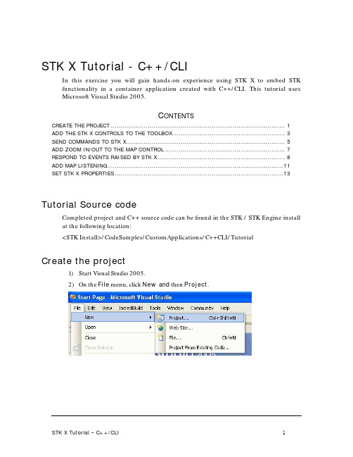
Tutorial Source code

Practice CS 基本安装指南说明书

PRACTICE CS INSTALLATION INSTRUCTIONSInstalling Practice CS (1)Downloading and installing the license (2)Obtaining and installing licenses via CS Connect (2)Installing licenses received via email (2)Running desktop setup (for network installations only) (3)Use this document to do the following:▪install Practice CS®▪download and install the license and software updates, and▪run desktop setup (for network installations only)Installing Practice CSYou can install Practice CS to a network or to a standalone computer using the product installation file downloaded from our website or from a CD.Notes▪The installation process may require you to restart the computer. If you are installing the program ona network, be sure that all other users have logged off the network.▪Installation must be performed at the computer that you want to designate as the Database Server.▪The computer where the shared files are installed must be turned on in order for the program files to be available to users (workstations).1. From the computer on which the database will reside, verify that you are logged in to your computeror server as an administrator.2. Close all open applications, including background virus protection software.3. Do one of the following:▪If you downloaded the product installation file from our website — Navigate to and double-click the EXE file that you downloaded to extract the files to the default folder (C:\Practice CS<version> Download) or to another folder of your choosing. If the installation wizard does not start automatically, navigate to the folder to which you extracted the files and double-click Setup.exe.▪If you are installing from a CD — Insert the CD into the disc drive on your computer. If the installation program does not start automatically, click Start on the Windows taskbar, choose Run, enter the command D:\SETUP (where D represents the letter of your disc drive), and click OK. 4. When Practice CS Setup starts, click the Install Practice CS link. The wizard will guide you throughthe rest of the installation.5. Practice CS uses Microsoft® SQL Server® (including 2008 Express Edition and later) for storing data.The computer on which the data is located (the SQL server) must be turned on in order for others to access the data. In addition, you must create an exception within the firewall for the instance of SQLServer you are using (recommended) or disable the firewall (not recommended) to run Practice CS. If you need assistance in creating an exception for the instance of SQL Server you are using, please refer to your firewall’s documentation or Microsoft knowledgebase article ID 841251(/kb/841251/).Downloading and installing the licenseAfter you install the program files, use CS Connect™ to download and install the license. In rare cases, you may receive a license file via email. If you received a license file via email, please skip the following procedure and proceed to “Installing licenses received via email” on page 2. Otherwise, complete the following procedure to install the licenses for your Practice CS software.Obtaining and installing licenses via CS ConnectComplete the following procedure to open Practice CS and use CS Connect to obtain and install the licenses electronically.1. Verify that you are logged in to your computer or server as an administrator.2. Start Practice CS.3. Click Cancel to close the login dialog.4. To open CS Connect, choose Help > About Practice CS, and click the Download Licenses button.5. Enter your firm ID (listed on your CS web account and on your mailing label) and your firm mailingaddress ZIP code, or PIN, and click Next.Note: If the Connect – Communications Setup dialog opens, verify or select the applicablecommunications settings, and then click OK to close the dialog.6. In the CS Connect dialog, click OK. CS Connect logs in to the Thomson Reuters data center anddownloads your licenses.7. Follow the remaining prompts to install the licenses.Installing licenses received via email1. If you received a Practice CS license file via email, please follow the instructions in that emailmessage and then follow the steps below.2. The installation wizard prompts you to choose the destination location for Practice CS. You need tochoose the folder where the shared files are installed. (The final destination for the program should bea folder called \WINCSI. For example, you may have installed your shared files in F:\APPS\WINCSI.)3. After you have verified the destination path, click Next to continue with the installation.Important! Even if you received your original license files via email, all updates to your Practice CS license information are available only via CS Connect. If you require an updated license in the future (for example, if you purchase a license for an optional add-on module later), you will need to download and install the updated license via CS Connect, as described in “Obtaining and installing licenses via CS Connect” on page 2.Running desktop setup (for network installations only) Important! If you installed the shared files on a network, you must also run the desktop setup program on each workstation.The desktop setup program ensures that each workstation meets the minimum operating system requirements and confirms that all required components are installed. When you run the desktop setup program, a shortcut to the single network installation of Practice CS (on your firm’s server) is added to each desktop. This keeps all firm-wide files and data in a single location on the server. We recommend that network users do not install the full program on their local computers.1. Verify that you are logged in to your computer as an administrator.2. Close all open applications.3. Click Start on the Windows taskbar and choose Run.4. In the Run dialog, enter Z:\path\Practice CS\Desktop\Setup.exe (where Z represents the mappeddrive letter for the network path to the server on which you installed the shared files, and path is the path to your Practice CS folder). For example, if you installed the shared files inF:\WINAPPS\WINCSI, you would need to enter F:\WINAPPS\WINCSI\Practice CS\Desktop\Setup.exe in the Run dialog or \\<name of server>\WINAPPS\WINCSI\Practice CS\Desktop\Setup.exe.Note: If you need to uninstall the Practice CS desktop setup from a workstation, choose Start > Settings > Control Panel > Add/Remove Programs, select Practice CS, and then click theChange/Remove button.5. Click OK and follow the prompts.6. Remote Entry requires a local installation of Microsoft SQL Server, version 2008 or later. If you choseto enable Remote Entry, you will be prompted to select an existing instance of SQL Server, or to install a new instance. Select an existing instance of SQL Server to use for Remote Entry, or click the option to install a new instance. Then click Next.7. When prompted that the Practice CS setup has been successfully completed, click Finish.。

Ansys Fluent 13.0 or 14.0 Tutorials教程

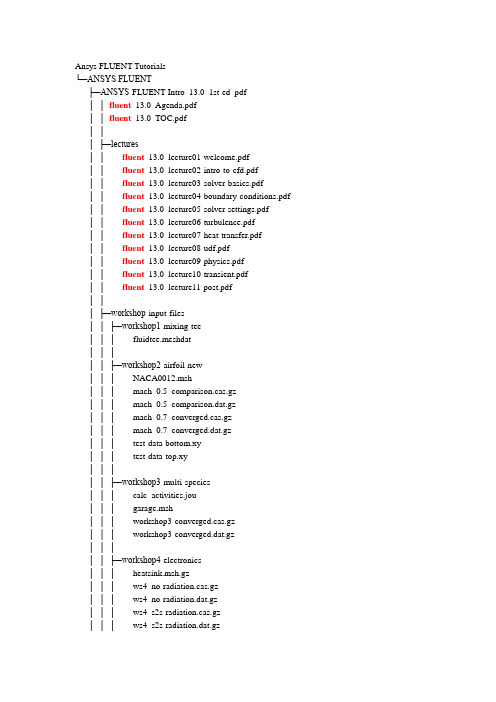
Ansys FLUENT Tutorials└─ANSYS FLUENT├─ANSYS-FLUENT-Intro_13.0_1st-ed_pdf││fluent_13.0_Agenda.pdf││fluent_13.0_TOC.pdf│││├─lectures││fluent_13.0_lecture01-welcome.pdf││fluent_13.0_lecture02-intro-to-cfd.pdf││fluent_13.0_lecture03-solver-basics.pdf││fluent_13.0_lecture04-boundary-conditions.pdf ││fluent_13.0_lecture05-solver-settings.pdf││fluent_13.0_lecture06-turbulence.pdf││fluent_13.0_lecture07-heat-transfer.pdf││fluent_13.0_lecture08-udf.pdf││fluent_13.0_lecture09-physics.pdf││fluent_13.0_lecture10-transient.pdf││fluent_13.0_lecture11-post.pdf│││├─workshop-input-files││├─workshop1-mixing-tee│││ fluidtee.meshdat│││││├─workshop2-airfoil-new│││ NACA0012.msh│││ mach_0.5_comparison.cas.gz│││ mach_0.5_comparison.dat.gz│││ mach_0.7_converged.cas.gz│││ mach_0.7_converged.dat.gz│││ test-data-bottom.xy│││ test-data-top.xy│││││├─workshop3-multi-species│││ calc_activities.jou│││ garage.msh│││ workshop3-converged.cas.gz│││ workshop3-converged.dat.gz│││││├─workshop4-electronics│││ heatsink.msh.gz│││ ws4_no-radiation.cas.gz│││ ws4_no-radiation.dat.gz│││ ws4_s2s-radiation.cas.gz│││ ws4_s2s-radiation.dat.gz│││ ws4_viewfactor.s2s.gz│││││├─workshop5-moving-parts│││ ws5-mesh-animation.avi│││ ws5-simple-wind-turbine.msh│││ ws5_udf_for_motion.c│││││├─workshop6-dpm│││ dpm_tutorial.msh│││││└─workshop7-tank-flush││tankflush.msh.gz││ws7-tankflush-animation.avi││ws7-tankflush-animation.mpeg│││└─workshops│fluent_13.0_WS_TOC.pdf│fluent_13.0_workshop01-mixingtee.pdf│fluent_13.0_workshop02-airfoil.pdf│fluent_13.0_workshop03-Multiple-Species.pdf│fluent_13.0_workshop04-electronics.pdf│fluent_13.0_workshop05-moving-parts.pdf│fluent_13.0_workshop06-dpm.pdf│fluent_13.0_workshop07-tank-flush.pdf│├─Quick Tutorials││ FLUENT_Overview_1_Introduction_to_FLUENT12_in_ANSYS_Workbench_DOC.pd f││ FLUENT_Overview_1_Introduction_to_FLUENT12_in_ANSYS_Workbench_WA TCH ME.swf││ FLUENT_Overview_2_Creating_and_Comparing_Related_FLUENT12_Analyses_in_ ANSYS_Workbench_DOC.pdf││ FLUENT_Overview_2_Creating_and_Comparing_Related_FLUENT12_Analyses_in_ ANSYS_Workbench_WA TCHME.swf││ FLUENT_Overview_3_Parametric_Study_Using_FLUENT12_in_ANSYS_Workbench _DOC.pdf││ FLUENT_Overview_3_Parametric_Study_Using_FLUENT12_in_ANSYS_Workbench _WATCHME.swf││ FLUENT_Overview_4_1-Way_Fluid-Structure_Interaction_Using_FLUENT12_and_A NSYS_Mechanical_DOC.pdf││ FLUENT_Overview_4_1-Way_Fluid-Structure_Interaction_Using_FLUENT12_and_A NSYS_Mechanical_WA TCHME.swf│││├─FLUENT_Overview_1_FILES││ probe.agdb│││├─FLUENT_Overview_2_FILES│││ Duplicate_Probe_Fluent.wbpj│││││└─Duplicate_Probe_Fluent_files│││ .project_cache│││││├─dp0││││ designPoint.wbdp│││││││├─FFF││││├─DM│││││ FFF.agdb│││││││││├─Fluent│││││ FFF-1-00100.dat.gz│││││ FFF-1.cas.gz│││││ FFF.set│││││││││├─MECH│││││ FFF.msh│││││││││└─Post││││Probe.cst│││││││├─FFF-1││││└─Fluent││││FFF-1.1-1-00081.dat.gz │││││││└─global│││└─MECH││││ FFF.mshdb│││││││└─FFF││└─user_files│├─FLUENT_Overview_3_FILES│││ Parametric_Probe_Fluent.wbpj│││││└─Parametric_Probe_Fluent_files│││ .project_cache│││││├─dp0││││ designPoint.wbdp│││││││├─FFF││││├─DM│││││ FFF.agdb│││││││││├─Fluent│││││ FFF-1-00100.dat.gz│││││ FFF-1.cas.gz│││││ FFF.set│││││││││├─MECH│││││ FFF.msh│││││││││└─Post││││Probe.cst│││││││├─FFF-1││││└─Fluent││││FFF-1.1-1-00081.dat.gz │││││││└─global│││└─MECH││││ FFF.mshdb│││││││└─FFF││└─user_files│└─FLUENT_Overview_4_FILES││ FSI_Probe_Fluent.wbpj│││└─FSI_P robe_Fluent_files││ .project_cache│││├─dp0│││ designPoint.wbdp│││││├─FFF│││├─DM││││ FFF.agdb│││││││├─Fluent││││ FFF-1-00100.dat.gz││││ FFF-1.cas.gz││││ FFF.set│││││││├─MECH││││ FFF.msh│││││││└─Post│││Probe.cst│││││├─FFF-1│││└─Fluent│││FFF-1.1-1-00081.dat.gz│││││└─global││└─MECH│││ FFF.mshdb│││││└─FFF│└─user_files├─combustion-fluent││ combustion-tutorial-list_13.0.pdf││ tut-01-intro-tut-16-species-transport.pdf││ tut-02-intro-tut-17-non-premix-combustion.pdf ││ tut-03-intro-tut-18-surface-chemistry.pdf││ tut-04-intro-tut-19-evaporating-liquid.pdf││ tut-05-berl.pdf││ tut-06-finite-rate.pdf││ tut-07-pdf-jet.pdf││ tut-08-cijr.pdf││ tut-09-pilot-jet.pdf││ tut-10-zimont.pdf││ tut-11-surfchem.pdf││ tut-12-mchar.pdf││ tut-13-co-combustor.pdf││ tut-14-flamelet.pdf││ tut-15-moss-brookes.pdf││ tut-16-dqmom.pdf││ tut-17-species.pdf││ tut-18-euler-granular.pdf││ tut-19-dpm-channel.pdf│││├─tut-01-intro-tut-16-species-transport│││ gascomb.msh│││││└─solution_files││gascomb1.cas.gz││gascomb1.dat.gz││gascomb2.dat.gz││gascomb3.cas.gz││gascomb3.dat.gz│││├─tut-02-intro-tut-17-non-premix-combustion │││ berl.msh│││ berl.prof│││││└─solution_files││berl-1.cas.gz││berl-1.dat.gz││berl.pdf│││├─tut-03-intro-tut-18-surface-chemistry│││ surface.msh│││││└─solution_files││surface-non-react.cas.gz││surface-react1.cas.gz││surface-react1.dat.gz││surface-react2.cas.gz││surface-react2.dat.gz│││├─tut-04-intro-tut-19-evaporating-liquid│││ sector.msh│││││└─solution_files││sector.msh││spray1.cas.gz││spray1.dat.gz││spray2.cas.gz││spray2.dat.gz││spray3.cas.gz││spray3.dat.gz│││├─tut-05-berl│││ berl.msh.gz│││ berl.prof│││││└─solution_files││berl-mag-1.cas.gz││berl-mag-1.dat.gz││berl-mag-2.cas.gz││berl-mag-3.cas.gz ││berl-mag-3.dat.gz │││├─tut-06-finite-rate│││ conreac.msh.gz│││││└─solution_files││5step.cas.gz││5step.dat.gz││5step_cold.cas.gz ││5step_cold.dat.gz ││5step_final.cas.gz │││├─tut-07-pdf-jet│││ CH4-skel.che│││ flameD.msh.gz│││ therm.dat│││││└─solution_files││flameD-1.cas.gz ││flameD-1.dat.gz ││flameD-2.cas.gz ││flameD-2.dat.gz ││flameD-3.cas.gz ││flameD-3.dat.gz ││flameD.pdf.gz││surf-mon-1.out │││├─tut-08-cijr│││ CIJR-therm.dat│││ CIJR.che│││ CIJR.msh.gz│││││└─solution_files││CIJR-1.cas.gz││CIJR-1.dat.gz││CIJR-2.cas.gz││CIJR-2.dat.gz││CIJR-3.cas.gz││CIJR-3.dat.gz││CIJR-4.cas.gz││CIJR-4.dat.gz││CIJR-4.fla.gz││CIJR.fla.gz││CIJR.pdf.gz││CIJRdisplay.cas.gz ││CIJRdisplay.dat.gz │││├─tut-09-pilot-jet│││ flameD-sfla.msh.gz│││ gri30.che│││││└─solution_files││flameD-sfla-1.cas.gz ││flameD-sfla-1.dat.gz ││flameD-sfla.fla.gz ││flameD-sfla.pdf.gz ││flameD-ufla-1.cas.gz ││flameD-ufla-1.dat.gz ││flameD-ufla-1.fla.gz ││surf-mon-1.out│││├─tut-10-zimont│││ conreac.msh│││││└─solution_files││zimont-ad.cas.gz││zimont-ad.dat.gz││zimont-nonad.cas.gz ││zimont-nonad.dat.gz ││zimont.cas.gz│││├─tut-11-surfchem│││ gas_chem.che│││ surf_chem.che│││ test.msh.gz│││││└─solution_files││surf-cat-comb.cas.gz ││surf-cat-comb.dat.gz ││surf-mon-1.out│││├─tu t-12-mchar│││ mchar.msh.gz│││││└─solution_files││mchar-rad.cas.gz││mchar-rad.dat.gz││mchar.cas.gz││mchar.dat.gz││view-0.vw│││├─tut-13-co-combustor│││ par-premixed.msh.gz│││││└─solution_files││par-premixed.pdf.gz││peters-partially-premixed-2nd.cas.gz ││peters-partially-premixed-2nd.dat.gz ││zimont-partially-premixed-1st.cas.gz ││zimont-partially-premixed-1st.dat.gz ││zimont-partially-premixed-2nd.cas.gz ││zimont-partially-premixed-2nd.dat.gz ││zimont-partially-premixed.cas.gz││zimont-partially-premixed.dat.gz│││├─tut-14-flamelet│││ berl.msh.gz│││ berl.prof│││ smooke46.che│││ thermo.db│││││└─solution_files││berl-converged.cas.gz││berl-converged.dat.gz││berl-ini.cas.gz││berl-second.cas.gz││berl-second.dat.gz││berl.fla.gz││berl.pdf.gz│││├─tut-15-moss-brookes│││ brookes_ch4.cas.gz│││ brookes_ch4.dat.gz│││ brookes_ch4.pdf.gz│││ brookes_ch4.ray│││ flamlet.fla│││ therm.dat│││││└─solution_files││brookes_ch4_soot_converged.cas.gz││brookes_ch4_soot_converged.dat.gz │││├─tut-16-dqmom│││ dqmom.msh.gz│││││└─solution_files││dqmom-1.cas.gz││dqmom-1.dat.gz││dqmom-2.cas.gz││dqmom-2.dat.gz││dqmom-final.cas.gz││dqmom-final.dat.gz││dqmom-init.cas.gz││dqmom-init.dat.gz││dqmom.cas.gz││dqmom.dat.gz│││├─tut-17-species│││ baffled_reactor.msh.gz│││││└─solution_files││case-1-rtd-complete.cas.gz││case-1-rtd-complete.dat.gz││case-1-tracer-init.cas.gz││case-1-tracer-init.dat.gz││case-1-tracer-injection-complete.cas.gz ││case-1-tracer-injection-complete.dat.gz ││case-1-tracer.out││case-1.cas.gz││case-1.dat.gz││case-2-rtd-complete.cas.gz││case-2-rtd-complete.dat.gz││case-2-rtd-final.cas.gz││case-2-rtd-final.dat.gz││case-2-tracer-init.cas.gz││case-2-tracer-init.dat.gz││case-2-tracer-injection-complete.cas.gz ││case-2-tracer-injection-complete.dat.gz ││case-2-tracer.out││case-2.cas.gz││case-2.dat.gz││surf-mon-1.out│││├─tut-18-euler-granular│││ euler.msh.gz│││ mass_xfer_rate.c│││││└─solution_files││euler-gran-1.cas.gz││euler-gran-1.dat.gz││euler-gran-final.cas.gz││euler-gran-final.dat.gz││vol-solid.out│││└─tut-19-dpm-channel││ 3dpipe.msh.gz│││└─solution_files│ dpm-evap.cas.gz│ dpm-evap.dat.gz│ pipe-flow.cas.gz│ pipe-flow.dat.gz│├─extra││ FLUENT13_workshop_XX_RAE_Airfoil.pptx ││ FLUENT13_workshop_XX_V ortexShedding.pptx │││├─workshop_XX_RAE_Airfoil│││ ExperimentalData.csv│││ coarse.xy│││ experiment.xy│││ expressions.cst│││ rae2822_coarse.msh│││││└─Result_TUT_04│││ rae2822_coarse-data_export_to_post.cas │││ rae2822_coarse-data_export_to_post.cdat │││ rae2822_coarse-data_export_to_post.cst│││ rae2822_coarse.cas.gz│││ rae2822_coarse.dat.gz│││││└─FINE_MESH││ medium.xy││ rae2822_fine.cas.gz││ rae2822_fine.dat.gz││ rae2822_fine.msh││ rae2822_medium.cas.gz││ rae2822_medium.dat.gz││ rae2822_medium.msh│││└─workshop_XX_V ortexShedding││ point-4-y-velocity-final.out││ vortex-shedding-coarse.msh││ vortex-shedding-unsteady.cas.gz││ vortex-shedding-unsteady.dat.gz│││├─FILES_FOR_CFDPOST││ vectors.mp4││ vortex-shedding-unsteady-3-68.949997.dat.gz ││ vortex-shedding-unsteady-3-69.199997.dat.gz ││ vortex-shedding-unsteady-3-69.449997.dat.gz ││ vortex-shedding-unsteady-3-69.699997.dat.gz ││ vortex-shedding-unsteady-3-69.949997.dat.gz ││ vortex-shedding-unsteady-3-70.199997.dat.gz ││ vortex-shedding-unsteady-3-70.449997.dat.gz ││ vortex-shedding-unsteady-3-70.699997.dat.gz ││ vortex-shedding-unsteady-3-70.949997.dat.gz ││ vortex-shedding-unsteady-3-71.199997.dat.gz ││ vortex-shedding-unsteady-3-71.449997.dat.gz ││ vortex-shedding-unsteady-3-71.699997.dat.gz ││ vortex-shedding-unsteady-3-71.949997.dat.gz ││ vortex-shedding-unsteady-3-72.199997.dat.gz ││ vortex-shedding-unsteady-3-72.449997.dat.gz ││ vortex-shedding-unsteady-3-72.699997.dat.gz ││ vortex-shedding-unsteady-3-72.949997.dat.gz ││ vortex-shedding-unsteady-3-73.199997.dat.gz ││ vortex-shedding-unsteady-3-73.449997.dat.gz ││ vortex-shedding-unsteady-3-73.699997.dat.gz ││ vortex-shedding-unsteady-3-73.949997.dat.gz ││ vortex-shedding-unsteady-3-74.199997.dat.gz ││ vortex-shedding-unsteady-3-74.449997.dat.gz ││ vortex-shedding-unsteady-3-74.699997.dat.gz ││ vortex-shedding-unsteady-3-74.949997.dat.gz ││ vortex-shedding-unsteady-3-75.199997.dat.gz ││ vortex-shedding-unsteady-3-75.449997.dat.gz ││ vortex-shedding-unsteady-3-75.699997.dat.gz ││ vortex-shedding-unsteady-3-75.949997.dat.gz ││ vortex-shedding-unsteady-3-76.199997.dat.gz ││ vortex-shedding-unsteady-3-76.449997.dat.gz ││ vortex-shedding-unsteady-3-76.699997.dat.gz ││ vortex-shedding-unsteady-3-76.949997.dat.gz ││ vortex-shedding-unsteady-3-77.199997.dat.gz││ vortex-shedding-unsteady-3-77.699997.dat.gz ││ vortex-shedding-unsteady-3-77.949997.dat.gz ││ vortex-shedding-unsteady-3-78.199997.dat.gz ││ vortex-shedding-unsteady-3-78.449997.dat.gz ││ vortex-shedding-unsteady-3-78.699997.dat.gz ││ vortex-shedding-unsteady-3-78.949997.dat.gz ││ vortex-shedding-unsteady-3-79.199997.dat.gz ││ vortex-shedding-unsteady-3-79.449997.dat.gz ││ vortex-shedding-unsteady-3-79.699997.dat.gz ││ vortex-shedding-unsteady-3-79.949997.dat.gz ││ vortex-shedding-unsteady-3-80.199997.dat.gz ││ vortex-shedding-unsteady-3-80.449997.dat.gz ││ vortex-shedding-unsteady-3-80.699997.dat.gz ││ vortex-shedding-unsteady-3-80.950012.dat.gz ││ vortex-shedding-unsteady-3-81.200027.dat.gz ││ vortex-shedding-unsteady-3-81.450043.dat.gz ││ vortex-shedding-unsteady-3-81.700058.dat.gz ││ vortex-shedding-unsteady-3-81.950073.dat.gz ││ vortex-shedding-unsteady-3-82.200089.dat.gz ││ vortex-shedding-unsteady-3-82.450104.dat.gz ││ vortex-shedding-unsteady-3-82.700119.dat.gz ││ vortex-shedding-unsteady-3-82.950134.dat.gz ││ vortex-shedding-unsteady-3-83.200150.dat.gz ││ vortex-shedding-unsteady-3-83.450165.dat.gz ││ vortex-shedding-unsteady-3-83.700180.dat.gz ││ vortex-shedding-unsteady-3-83.950195.dat.gz ││ vortex-shedding-unsteady-3-84.200211.dat.gz ││ vortex-shedding-unsteady-3-84.450226.dat.gz ││ vortex-shedding-unsteady-3-84.700241.dat.gz ││ vortex-shedding-unsteady-3-84.950256.dat.gz ││ vortex-shedding-unsteady-3-85.200272.dat.gz ││ vortex-shedding-unsteady-3-85.450287.dat.gz ││ vortex-shedding-unsteady-3-85.700302.dat.gz ││ vortex-shedding-unsteady-3-85.950317.dat.gz ││ vortex-shedding-unsteady-3-86.200333.dat.gz ││ vortex-shedding-unsteady-3-86.450348.dat.gz ││ vortex-shedding-unsteady-3-86.700363.dat.gz ││ vortex-shedding-unsteady-3-86.950378.dat.gz ││ vortex-shedding-unsteady-3-87.200394.dat.gz ││ vortex-shedding-unsteady-3-87.450409.dat.gz ││ vortex-shedding-unsteady-3-87.700424.dat.gz ││ vortex-shedding-unsteady-3-87.950439.dat.gz ││ vortex-shedding-unsteady-3-88.200455.dat.gz││ vortex-shedding-unsteady-3-88.700485.dat.gz ││ vortex-shedding-unsteady-3-88.950500.dat.gz ││ vortex-shedding-unsteady-3-89.200516.dat.gz ││ vortex-shedding-unsteady-3-89.450531.dat.gz ││ vortex-shedding-unsteady-3-89.700546.dat.gz ││ vortex-shedding-unsteady-3-89.950562.dat.gz ││ vortex-shedding-unsteady-3-90.200577.dat.gz ││ vortex-shedding-unsteady-3-90.450592.dat.gz ││ vortex-shedding-unsteady-3-90.700607.dat.gz ││ vortex-shedding-unsteady-3-90.950623.dat.gz ││ vortex-shedding-unsteady-3-91.200638.dat.gz ││ vortex-shedding-unsteady-3-91.450653.dat.gz ││ vortex-shedding-unsteady-3-91.700668.dat.gz ││ vortex-shedding-unsteady-3-91.950684.dat.gz ││ vortex-shedding-unsteady-3-92.200699.dat.gz ││ vortex-shedding-unsteady-3-92.450714.dat.gz ││ vortex-shedding-unsteady-3-92.700729.dat.gz ││ vortex-shedding-unsteady-3.cas.gz│││└─Result-TUT_07││ cfd_post.cst││ point-4-y-velocity-final.out││ point-4-y-velocity.out││ sequence-1.mpeg││ vectors.mp4││ vortex-shedding-coarse-steady.cas.gz││ vortex-shedding-coarse-steady.dat.gz││ vortex-shedding-unsteady-final.cas.gz││ vortex-shedding-unsteady-final.dat.gz││ vortex-shedding-unsteady.cas.gz││ vortex-shedding-unsteady.dat.gz│││├─ADDITIONAL-FILES││ q-criterion2D.scm││ velocity.fft│││└─ANIMATION-FILES│ sequence-1.cxa│ sequence-1.mpeg│ sequence-1_0000.hmf│ sequence-1_0001.hmf│ sequence-1_0002.hmf│ sequence-1_0003.hmf│ sequence-1_0005.hmf │ sequence-1_0006.hmf │ sequence-1_0007.hmf │ sequence-1_0008.hmf │ sequence-1_0009.hmf │ sequence-1_0010.hmf │ sequence-1_0011.hmf │ sequence-1_0012.hmf │ sequence-1_0013.hmf │ sequence-1_0014.hmf │ sequence-1_0015.hmf │ sequence-1_0016.hmf │ sequence-1_0017.hmf │ sequence-1_0018.hmf │ sequence-1_0019.hmf │ sequence-1_0020.hmf │ sequence-1_0021.hmf │ sequence-1_0022.hmf │ sequence-1_0023.hmf │ sequence-1_0024.hmf │ sequence-1_0025.hmf │ sequence-1_0026.hmf │ sequence-1_0027.hmf │ sequence-1_0028.hmf │ sequence-1_0029.hmf │ sequence-1_0030.hmf │ sequence-1_0031.hmf │ sequence-1_0032.hmf │ sequence-1_0033.hmf │ sequence-1_0034.hmf │ sequence-1_0035.hmf │ sequence-1_0036.hmf │ sequence-1_0037.hmf │ sequence-1_0038.hmf │ sequence-1_0039.hmf │ sequence-1_0040.hmf │ sequence-1_0041.hmf │ sequence-1_0042.hmf │ sequence-1_0043.hmf │ sequence-1_0044.hmf │ sequence-1_0045.hmf │ sequence-1_0046.hmf │ sequence-1_0047.hmf│ sequence-1_0049.hmf │ sequence-1_0050.hmf │ sequence-1_0051.hmf │ sequence-1_0052.hmf │ sequence-1_0053.hmf │ sequence-1_0054.hmf │ sequence-1_0055.hmf │ sequence-1_0056.hmf │ sequence-1_0057.hmf │ sequence-1_0058.hmf │ sequence-1_0059.hmf │ sequence-1_0060.hmf │ sequence-1_0061.hmf │ sequence-1_0062.hmf │ sequence-1_0063.hmf │ sequence-1_0064.hmf │ sequence-1_0065.hmf │ sequence-1_0066.hmf │ sequence-1_0067.hmf │ sequence-1_0068.hmf │ sequence-1_0069.hmf │ sequence-1_0070.hmf │ sequence-1_0071.hmf │ sequence-1_0072.hmf │ sequence-1_0073.hmf │ sequence-1_0074.hmf │ sequence-1_0075.hmf │ sequence-1_0076.hmf │ sequence-1_0077.hmf │ sequence-1_0078.hmf │ sequence-1_0079.hmf │ sequence-1_0080.hmf │ sequence-1_0081.hmf │ sequence-1_0082.hmf │ sequence-1_0083.hmf │ sequence-1_0084.hmf │ sequence-1_0085.hmf │ sequence-1_0086.hmf │ sequence-1_0087.hmf │ sequence-1_0088.hmf │ sequence-1_0089.hmf │ sequence-1_0090.hmf │ sequence-1_0091.hmf│ sequence-1_0093.hmf│ sequence-1_0094.hmf│ sequence-1_0095.hmf│ sequence-1_0096.hmf│ sequence-1_0097.hmf│ sequence-1_0098.hmf│ sequence-1_0099.hmf│ sequence-1_0100.hmf│ sequence-1_0101.hmf│ sequence-1_0102.hmf│ sequence-1_0103.hmf│ sequence-1_0104.hmf│ sequence-1_0105.hmf│ sequence-1_0106.hmf│ sequence-1_0107.hmf│ sequence-1_0108.hmf│ sequence-1_0109.hmf│ sequence-1_0110.hmf│ sequence-1_0111.hmf│ sequence-1_0112.hmf│ sequence-1_0113.hmf│ sequence-1_0114.hmf│ sequence-1_0115.hmf│ sequence-1_0116.hmf│ sequence-1_0117.hmf│ sequence-1_0118.hmf│ sequence-1_0119.hmf│├─fluent-heat-transfer││ ht-01-intro-tut-04-periodic-flow-heat.pdf││ ht-02-intro-tut-07-radiation-and-convection.pdf ││ ht-03-intro-tut-08-DO-radiation.pdf││ ht-04-intro-tut-24-solidification.pdf││ ht-05-conjugate-heat-transfer.pdf││ ht-06-compact-heat-exchanger.pdf││ ht-07-macro-heat-exchanger.pdf││ ht-08-head-lamp.pdf│││├─ht-01-intro-tut-04-periodic-flow-heat│││ tubebank.msh│││││└─solution_files││tubebank.cas.gz││tubebank.dat.gz│││├─ht-02-intro-tut-07-radiation-and-convection │││ rad.msh.gz│││││└─solution_files││rad_1.s2s.gz││rad_10.cas.gz││rad_10.dat.gz││rad_10.s2s.gz││rad_100.cas.gz││rad_100.dat.gz││rad_100.s2s.gz││rad_1600.cas.gz││rad_1600.dat.gz││rad_1600.s2s.gz││rad_400.cas.gz││rad_400.dat.gz││rad_400.s2s.gz││rad_800.cas.gz││rad_800.dat.gz││rad_800.s2s.gz││rad_a_1.cas.gz││rad_b_1.cas.gz││rad_b_1.dat.gz││rad_partial.cas.gz││rad_partial.dat.gz││rad_partial.s2s.gz││tp_1.xy││tp_10.xy││tp_100.xy││tp_1600.xy││tp_400.xy││tp_800.xy││tp_partial.xy│││├─ht-03-intro-tut-08-DO-radiation│││ do.msh.gz│││││└─solution_files││do.cas.gz││do.dat.gz││do_2x2_10x10_pix.cas.gz││do_2x2_10x10_pix.dat.gz││do_2x2_1x1.xy││do_2x2_2x2_pix.cas.gz││do_2x2_2x2_pix.dat.gz││do_2x2_2x2_pix.xy││do_2x2_3x3_div.cas.gz││do_2x2_3x3_div.dat.gz││do_2x2_3x3_div.xy││do_2x2_3x3_pix.cas.gz││do_2x2_3x3_pix.dat.gz││do_2x2_3x3_pix.xy││do_3x3_3x3_div.cas.gz││do_3x3_3x3_div.dat.gz││do_3x3_3x3_div.xy││do_3x3_3x3_div_baf_int.xy ││do_3x3_3x3_div_df1.cas.gz ││do_3x3_3x3_div_df1.dat.gz ││do_3x3_3x3_div_df=1.xy ││do_3x3_3x3_div_int.cas.gz ││do_3x3_3x3_div_int.dat.gz ││do_5x5_3x3_div.cas.gz││do_5x5_3x3_div.dat.gz││do_5x5_3x3_div.xy│││├─ht-04-intro-tut-24-solidification│││ solid.msh│││││└─solution_files││solid.cas.gz││solid.dat.gz││solid0.cas.gz││solid0.dat.gz││solid01.cas.gz││solid01.dat.gz││solid5.cas.gz││solid5.dat.gz│││├─ht-05-conjugate-heat-transfer│││ chip3d.msh.gz│││││└─solution_files││chip3d-adapt1.cas.gz││chip3d-adapt1.dat.gz││chip3d-adapt2.cas.gz││chip3d.cas.gz││chip3d.dat.gz││surf-mon-1.out││temp-0.xy││temp-1.xy││temp-2.xy││velocity-0.xy││velocity-1.xy││velocity-2.xy││xwss-0.xy││xwss-1.xy││xwss-2.xy│││├─ht-06-compact-heat-exchanger │││ htx.msh.gz│││││└─solution_files││htx-energy.cas.gz││htx-energy.dat.gz││htx-eqn.cas.gz││htx-eqn.dat.gz││htx-final.cas.gz││htx-final.dat.gz││htx-setup.cas.gz││htx-setup.dat.gz││surf-mon-1.out│││├─ht-07-macro-heat-exchanger │││ rad.tab│││ wedge.msh.gz│││││└─solution_files││wedge1.cas.gz││wedge1.dat.gz││wedge2.cas.gz││wedge2.dat.gz││wedge3.cas.gz││wedge3.dat.gz││wedge4.cas.gz││wedge4.dat.gz│││└─ht-08-head-lamp││ head-lamp.msh.gz│││└─solution_fi les│ auto-hlamp.cas.gz│ auto-hlamp.dat.gz│ head-lamp-t.out│ hed-lamp-v.out│├─multiphase-fluent││ 01-hfilm.pdf││ 02-boil.pdf││ 03-nucleate_boil.pdf││ 04-dambreak.pdf││ 05-sloshing.pdf││ 06-bubble-col.pdf││ 07-bubble-break.pdf││ 08-inkjet.pdf││ 09-sparger.pdf││ 10-pbed-reactor.pdf││ 11-ddpm.pdf││ 12-dm-ship-wave.pdf││ 13-udf-clarifier.pdf││ 14-udf-fbed.pdf│││├─tut-01-hfilm│││ boiling.c│││ test-2d.msh.gz│││││└─solution_files│││ hfilm_input_files.tar.zg │││ nusselt-1.out│││ test-2d-1-00100.dat│││ test-2d-1-00200.dat│││ test-2d-1-00300.dat│││ test-2d-1-00400.dat│││ test-2d-1-00500.dat│││ test-2d-1-00600.dat│││ test-2d-1-00700.dat│││ test-2d-1-00800.dat│││ test-2d-1-00900.dat│││ test-2d-1-01000.dat│││ test-2d-1-01100.dat│││ test-2d-1-01200.dat│││ test-2d-1-01300.dat│││ test-2d-1-01400.dat│││ test-2d-1-01500.dat│││ test-2d-1-01600.dat│││ test-2d-1-01700.dat│││ test-2d-1-01800.dat│││ test-2d-1-01900.dat│││ test-2d-1-02000.dat│││ test-2d-1-02100.dat│││ test-2d-1-02200.dat│││ test-2d-1-02300.dat│││ test-2d-1-02400.dat│││ test-2d-1-02500.dat│││ test-2d-1-02600.dat│││ test-2d-1-02700.dat│││ test-2d-1-02800.dat│││ test-2d-1-02900.dat│││ test-2d-1-03000.dat│││ test-2d-1-03100.dat│││ test-2d-1-03200.dat│││ test-2d-1-03300.dat│││ test-2d-1-03400.dat│││ test-2d-1-03500.dat│││ test-2d-1-03600.dat│││ test-2d-1-03700.dat│││ test-2d-1-03800.dat│││ test-2d-1-03900.dat│││ test-2d-1-04000.dat│││ test-2d-1.cas│││ vol-mon-1.out│││││└─libudf││├─ntx86│││└─2ddp│││boiling.obj│││libudf.dll│││libudf.exp│││libudf.lib│││log│││makefile│││udf_names.c │││udf_names.obj │││user_nt.udf│││││├─src│││ boiling.c│││││└─win64││└─2ddp││boiling.obj││libudf.dll││libudf.exp││libudf.lib││log││makefile││ud_io1.h││udf_names.c ││udf_names.obj ││user_nt.udf│││├─tut-02-boil│││ boil.msh.gz│││││└─solution_files││boil-3-00300.dat.gz││boil-3-01000.dat.gz││boil-3.cas.gz│││├─tut-03-nucleate-boil│││ boiling-conjugate.msh│││││└─solution_files││boil-final.cas.gz││boil-final.dat.gz││boil-init.cas.gz││boil-init.dat.gz││boil-single-phase.cas.gz ││boil-single-phase.dat.gz ││liquid-outlet.prof││surf-mon-1.out││surf-mon-2.out│││├─tut-04-dambreak│││ dambreak.msh.gz│││││└─solution_files││dambreak-100.cas.gz││dambreak-100.dat.gz││dambreak-50.cas.gz││dambreak-50.dat.gz││dambreak-80.cas.gz││dambreak-80.dat.gz││dambreak.cas.gz││dambreak.dat.gz│││├─tut-05-sloshing│││ ft11.msh.gz│││││└─solution_files││├─baffles│││ baffles-data-file-4-02060.dat.gz │││ baffles-data-file-4-02080.dat.gz │││ baffles-images.zip│││ baffles.jou│││ ft11.msh.gz│││ operating.cas.gz│││ t=0.0s.cas.gz│││ t=0.0s.dat.gz│││ t=0.45s.cas.gz│││ t=0.45s.dat.gz│││ t=1.25s.cas.gz│││ t=1.25s.dat.gz│││ t=1.50s.cas.gz│││ t=1.50s.dat.gz│││ t=1.5s.cas.gz│││ t=1.5s.dat.gz│││ t=2.5s.cas.gz│││ t=2.5s.dat.gz│││││└─no-baffles││ no-baffles-data-file-4-02760.dat.gz ││ no-baffles-data-file-4-02780.dat.gz ││ no-baffles-images.zip││ no-baffles.jou││ t=0.0s.cas.gz││ t=0.0s.dat.gz││ t=0.45s.cas.gz││ t=0.45s.dat.gz││ t=0s.cas.gz││ t=0s.dat.gz││ t=1.25s.cas.gz││ t=1.25s.dat.gz││ t=1.5s.cas.gz││ t=1.5s.dat.gz││ t=2.5s.cas.gz││ t=2.5s.dat.gz││ tiff-no-baffles.zip │││├─tut-06-bubble-col│││ becker.msh│││││└─solution_files││becker-1-00200.dat.gz ││becker-1-00400.dat.gz ││becker-1-00600.dat.gz ││becker-1-00800.dat.gz ││becker-1-01000.dat.gz ││becker-1-01200.dat.gz ││becker-1-01400.dat.gz ││becker-1-01600.dat.gz ││becker-1-01800.dat.gz ││becker-1-02000.dat.gz ││becker-1-02200.dat.gz ││becker-1-02400.dat.gz ││becker-1-02600.dat.gz ││becker-1-02800.dat.gz ││becker-1-03000.dat.gz ││becker-1-03200.dat.gz ││becker-1-03400.dat.gz ││becker-1-03600.dat.gz ││becker-1-03800.dat.gz ││becker-1-04000.dat.gz ││becker-1-04200.dat.gz ││becker-1-04400.dat.gz ││becker-1-04600.dat.gz ││becker-1-04800.dat.gz ││becker-1-05000.dat.gz ││becker-1.cas.gz││becker.cas.gz││becker.dat.gz││vel-vectors.cxa││vel-vectors_0000.hmf ││vel-vectors_0001.hmf ││vel-vectors_0002.hmf ││vel-vectors_0003.hmf ││vel-vectors_0004.hmf ││vel-vectors_0005.hmf ││vel-vectors_0006.hmf││vel-vectors_0007.hmf ││vel-vectors_0008.hmf ││vel-vectors_0009.hmf ││vel-vectors_0010.hmf ││vel-vectors_0011.hmf ││vel-vectors_0012.hmf ││vel-vectors_0013.hmf ││vel-vectors_0014.hmf ││vel-vectors_0015.hmf ││vel-vectors_0016.hmf ││vel-vectors_0017.hmf ││vel-vectors_0018.hmf ││vel-vectors_0019.hmf ││vel-vectors_0020.hmf ││vel-vectors_0021.hmf ││vel-vectors_0022.hmf ││vel-vectors_0023.hmf ││vel-vectors_0024.hmf ││vof.cxa││vof_0000.hmf││vof_0001.hmf││vof_0002.hmf││vof_0003.hmf││vof_0004.hmf││vof_0005.hmf││vof_0006.hmf││vof_0007.hmf││vof_0008.hmf││vof_0009.hmf││vof_0010.hmf││vof_0011.hmf││vof_0012.hmf││vof_0013.hmf││vof_0014.hmf││vof_0015.hmf││vof_0016.hmf││vof_0017.hmf││vof_0018.hmf││vof_0019.hmf││vof_0020.hmf││vof_0021.hmf││vof_0022.hmf││vof_0023.hmf││vof_0024.hmf│││├─tut-07-bubble-break│││ bubcol_new2.msh.gz│││││└─solution_files││bubcol-final.cas.gz││bubcol-final.dat.gz││bubcol_new2-initial.cas.gz ││bubcol_new2-initial.dat.gz ││surf-mon-1.out││surf-mon-2.out││surf-mon-3.out│││├─tut-08-inkjet│││ inkjet.msh.gz│││ inlet1.c│││ udfconfig.h│││││└─solution_files││inkjet-1-00100.dat.gz││inkjet-1-00200.dat.gz││inkjet-1-00300.dat.gz││inkjet-1-00400.dat.gz││inkjet-1-00500.dat.gz││inkjet-1-00600.dat.gz││inkjet-1-00700.dat.gz││inkjet-1-00800.dat.gz││inkjet-1-00900.dat.gz││inkjet-1-01000.dat.gz││inkjet-1-01100.dat.gz││inkjet-1-01200.dat.gz││inkjet-1-01300.dat.gz││inkjet-1-01400.dat.gz││inkjet-1-01500.dat.gz││inkjet-1.cas.gz││inkjet-final.cas.gz││inkjet-final.dat.gz││inkjet.cas.gz││inkjet.dat.gz│││├─tut-09-sparger│││ sparger.msh.gz│││││└─solution_files。

tutorial_xcrysden

XCRYSDEN: a short tutorial
... and its usage for PWscf !!!
Copy me ...
●
This tutorial can be downloaded from:
http://[ESPRESSO-TUTORIAL-SITE]/tutorial_xcrysden.pdf
Lighting On/Off display mode
●
VERY IMPORTANT !!!
–
two levels of display modes:
●
Lighting-Off mode:
–
very fast, but can display only atoms and bonds !!! more fancy display with shades, not so fast, but displays all possible items !!!
– – – –
●
●
modify number of displayed cells (Modify->Number of Units Drawn) change the unit of repetition (Display->Unit of Repetition ...->) display Wigner-Seitz cell (Display->Wigner-Seitz Cells) display Brillouin zone (Tools->k-path Selection)
( Note: requires the whirlgif and mpeg_encode programs to be defined in ~/.xcrysden/customdefinitions )

python-tutorial

This tutorial introduces the reader informally to the basic concepts and features of the Python language and system. It helps to have a Python interpreter handy for hands-on experience, but all examples are self-contained, so the tutorial can be read off-line as well.
The Python interpreter and the extensive standard library are freely available in source or binary form for all major platforms from the Python web site, , and can be freely distributed. The same site also contains distributions of and pointers to many free third party Python modules, programs and tools, and additional documentation.
CONTENTS
1 Whetting Your Appetite
1
1.1 Where From Here . . . . . . . . . . . . . . . . . . . . . . . . . . . . . . . . . . . . . . . . . . . . 2
2 Using the Python Interpreter

Qt Tutorial -中文版

Address Book 1 - Designing the User Interface Files:∙tutorials/addressbook/part1/addressbook.cpp∙tutorials/addressbook/part1/addressbook.h∙tutorials/addressbook/part1/main.cpp∙tutorials/addressbook/part1/part1.pro该教程第一部分覆盖了Address Book基本GUI的设计。

第一步创建的GUI程序是为了设计用户界面，本章中我们的目标是放置Labels标签和输入框来实现电话本的基本功能。

见下图：需要放置两个QLabel 对象，nameLabel1和addressLabel1,还有两个输入框，一个QLineEdit对象：nameLine，和一个QTextEdit对象：addressText，以便用户输入联系人姓名和地址。

见下图：有三类文件实习这个电话本程序：∙addressbook.h–定义∙addressbook.cpp–实现AddressBook类∙main.cpp–包含一个main()函数, 和一个AddressBook的实例Qt Programming - Subclassing当编写Qt程序时，我们通常继承Qt Objects来添加功能。

在创建自定义的widgets 或者一系列标准widgets时这是个重要的概念。

通过子类化改变widget的功能有以下优点：1. 可以实现虚函数或纯虚函数达到我们的需求，必要时也可以回调基类的功能。

2. 允许封装部分用户界面类，因此程序的其他部分不需要知道单独的组件如何工作3. 子类化可以在一个程序中创建不同的自定义组件，也可以在其他工程中复用。

Qt不支持特定的电话簿部件，所以我们通过继承Qt部件类来实现。

Defining the AddressBook Class通过定义Addressbook作为QWidget的子类并声明一个构造函数。

python基础教程英文版

python基础教程英文版A Python Basic Tutorial (English Version)。

Python is a widely-used high-level programming language known for its simplicity and readability. It is anexcellent choice for beginners who want to learn programming. In this tutorial, we will cover the basics of Python programming.1. Introduction to Python:Python is an interpreted language, which means that the code is executed line by line. It does not require a compilation step, making it easy to write and test code quickly.2. Installation:To get started with Python, you need to install the Python interpreter on your computer. You can download thelatest version of Python from the official website andfollow the installation instructions.3. Variables and Data Types:In Python, you can create variables to store data. Python supports various data types such as integers, floats, strings, booleans, lists, tuples, and dictionaries. Understanding these data types is crucial for writing effective code.4. Operators:Python provides a range of operators for performing arithmetic, comparison, logical, and assignment operations. These operators allow you to manipulate data and controlthe flow of your program.5. Control Flow:Control flow statements, such as if-else, for loops,and while loops, enable you to control the execution ofyour code based on certain conditions. These statements help in making decisions and iterating over data.6. Functions:Functions are reusable blocks of code that perform specific tasks. They help in organizing code and making it more modular. Python allows you to define and call functions, passing arguments and returning values.7. Modules and Packages:Python has a vast collection of built-in modules and packages that provide additional functionality. You can import these modules into your code and use their functions and classes. Additionally, you can create your own modules for code reusability.8. File Handling:Python provides various functions and methods for working with files. You can open, read, write, and closefiles using built-in file handling operations. Understanding file handling is essential for dealing with data stored in files.9. Exception Handling:Exception handling allows you to catch and handleerrors that may occur during the execution of your program. Python provides try-except blocks to handle exceptions gracefully and prevent your program from crashing.10. Object-Oriented Programming (OOP):Python supports object-oriented programming, which allows you to create classes and objects. OOP helps in organizing code and implementing complex systems byutilizing concepts such as inheritance, encapsulation, and polymorphism.11. Libraries and Frameworks:Python has a vast ecosystem of libraries and frameworksthat extend its capabilities. Libraries like NumPy, Pandas, and Matplotlib are widely used for scientific computing and data analysis. Frameworks like Django and Flask are popular for web development.12. Debugging and Testing:Python provides tools and techniques for debugging and testing your code. You can use debugging tools to find and fix errors in your program. Testing frameworks likeunittest and pytest help in writing automated tests to ensure the correctness of your code.In conclusion, this Python basic tutorial provides an overview of the fundamental concepts and features of the Python programming language. By understanding these concepts, you will be well-equipped to start writing your own Python programs and explore more advanced topics. Remember to practice writing code and experimenting with different examples to enhance your learning experience.。

python3.7.5官方tutorial学习笔记

python3.7.5官⽅tutorial学习笔记⽤了好久python，还没有完整看过官⽅的tutorial，这⼏天抽空看了下，还是学到些东西---Table of Contents1 课前甜点Python 代码通常⽐ C 系语⾔短的原因1. ⾼级数据类型允许在⼀个表达式中表⽰复杂的操作2. 代码块的划分是按照缩进3. 不需要预定义变量2 使⽤ Python 解释器2.1 调⽤解释器EOF unix C-d windows C-z执⾏ Python 代码 python -c command [arg]把 Python 模块当脚本使⽤ python -m module [arg]执⾏脚本后进⼊交互模式 python -i 1.py2.1.1 传⼊参数sys.argv sys.argv[0] 是程序名2.1.2 交互模式2.2 解释器的运⾏环境2.2.1 源⽂件的字符编码默认编码就是 utf-8 必须放在第⼀⾏或者 UNIX “shebang” 后3 Python 的⾮正式介绍注释 #3.1 Python 作为计算器使⽤3.1.1 数字除法 / 永远返回浮点数类型 // floor division乘⽅ **交互模式下,上⼀次被执⾏显⽰的表达式的值会被保存在 _Python 内置对复数的⽀持 3+5j3.1.2 字符串原始字符串三重引号会⾃动包含换⾏,可以在⾏尾加反斜杠防⽌换⾏相邻的两个字符串字⾯值会⾃动连接到⼀起通过索引取得的单个字符是⼀个长度为⼀的字符串切⽚中越界索引会被⾃动处理Python 中字符串是不可修改的,如果需要⼀个不同的字符串,应当新建⼀个 a = “heheda” b = a[:-1] + “b”3.1.3 列表列表的切⽚都返回⼀个新列表列表⽀持使⽤ + 拼接其他列表可以给列表切⽚赋值,这样可以改变列表⼤⼩,甚⾄清空整个列表a = [1, 2, 3, 4]a[1:3] = [4, 5]a[:] = []3.2 ⾛向编程的第⼀步3.2.1 多重赋值3.2.2 printprint 会在多个参数间加空格可以传⼊ end 参数指定结尾替换换⾏的字符串4 其他流程控制⼯具4.1 if 语句输⼊ aa = input(“input: ”)if if elif else4.2 for 语句Python 中的 for 是对任意序列进⾏迭代如果在循环内需要修改序列中的值,推荐先拷贝⼀份副本words = ['aaa', 'bbb', 'ccccccc']for w in words[:]:if len(w) > 5:words.insert(0, w)4.3 range() 函数range(0, 10, 3) 0, 3, 6, 9以序列的索引迭代a = ['a', 'b', 'c']for i in range(len(a)):print(i, a[i])for i, v in enumerate(a):print(i, v)range() 返回的不是列表,是⼀个可迭代对象4.4 break 和 continue 语句,以及循环中的 else ⼦句else ⼦句 else ⼦句会在未执⾏ break,循环结束时执⾏4.5 pass 语句pass 通常⽤于创建最⼩的类 class MyEmptyClass: passpass 也⽤于写代码时作为函数或条件⼦句体的占位符,保持在更抽象的层次上思考4.6 定义函数⽂档字符串全局变量和外部函数的变量可以被引⽤,但是不能在函数内部直接赋值函数的重命名机制没有 return, 函数会返回 None列表⽅法 append() ⽐ + 效率⾼4.7 函数定义的更多形式4.7.1 参数默认值in 测试⼀个序列是否包含某个值默认值时在定义过程中在函数定义处计算的,⽽不是调⽤时默认值只执⾏⼀次,如果是可变对象,⽐如列表,就可以在后续调⽤之间共享默认值类似于 c 中的静态变量def f(a, L=[]):print(a)L.append(a)print(L)f(1)f(2)f(3)f(4)4.7.2 关键字参数关键字参数必须在位置参数后形参 * **4.7.3 任意的参数列表任意的参数列表 *args ⼀般位于形式参数列表的末尾,只有关键字参数能出现在其后4.7.4 解包参数列表使⽤* 从列表或元组中解包参数 args = [3, 6] range(*args)使⽤** 从字典解包参数4.7.5 Lambda 表达式闭包def make_incrementor(n):return lambda x: x + nf = make_incrementor(33)f(0)传递⼀个函数作为参数pairs = [(1, 'one'), (2, 'two'), (3, 'three')]pairs.sort(key=lambda pair: pair[1])4.7.6 ⽂档字符串⼀些约定第⼀⾏简要描述对像的⽬的,⼤写字母开头,句点结尾第⼆⾏空⽩,后⾯⼏⾏是⼀个或多个段落,描述调⽤约定,副作⽤等4.7.7 函数标注标注不会对代码有实质影响,只是给⼈看def f(ham: str, eggs: str = "eggs") -> str:print(f.__annotations__)return ham + ' and ' + eggs4.8 ⼩插曲: 编码风格使⽤ 4 空格缩进,⽽不是制表符⼀⾏不超过 79 个字符(可以在较⼤显⽰器并排放置多个代码⽂件)使⽤空⾏分割函数和类,以及函数内的较⼤的代码块尽量把注释放到单独的⼀⾏使⽤⽂档字符串在运算符前后和逗号后使⽤空格函数和类命名应使⽤⼀致规则类 UpperCamelCase 函数 lowercase withunderscores⼀般不另外设置代码的编码不要在标识符中使⽤⾮ ASCII 字符5 数据结构5.1 列表的更多特性列表对象⽅法的清单 list.append(x) list.extend(iterable) list.insert(i, x) list.remove(x) list.pop([i]) list.clear() list.index(x[, start[, end]]) list.count(x) list.sort(key=None, reverse=False) list.reverse() list.copy()5.1.1 列表作为栈使⽤list.append(x) list.pop()5.1.2 列表作为队列使⽤在列表开头插⼊或弹出元素很慢from collections import dequequeue = deque(['aaa', 'bbb', 'ccc'])queue.append('ddd')queue.popleft()5.1.3 列表推导式for 循环后,循环变量还存在列表推导式中,for 和 if 顺序和展开形式的顺序是⼀致的如果表达式是⼀个元组,需要加括号5.1.4 嵌套的列表推导式a = [1, 2, 3]b = [4, 5, 6]print(list(zip(a, b)))5.2 del 语句del 可以删除指定索引的元素del 可以删除切⽚指定的范围del a[:]del a5.3 元组和序列元组通常包含不同种类的元素,列表的元素⼀般是同种类型空元组可以直接被⼀对圆括号创建元组输⼊时圆括号可有可⽆5.4 集合set()集合操作 a | b a - b a & b a ^ b集合推导式 a = {x for x in ’abcdedd’ if x not in ’abc’}5.5 字典只要不包含不可变对象,都可以作为键5.6 循环的技巧字典循环时,可以⽤ items() ⽅法把关键字和值同时取出序列循环时,可以⽤ enumerate()函数将索引和值同时取出要同时在多个序列中循环时,可以⽤ zip()函数如果要逆向⼀个序列,可以使⽤ reversed()函数sorted()函数可以返回⼀个新的排好序的序列在循环时想修改列表内容,最好创建新列表5.7 深⼊条件控制in 和 not inis 和 is not ⽐较是不是同⼀个对象⽐较操作可以传递5.8 ⽐较序列和其他类型序列也可以⽐较6 模块如果经常使⽤某个导⼊的函数,可以赋值给⼀个局部变量重命名6.1 更多有关模块的信息⼏种导⼊⽅式from fibo import fib, fib2from fibo import *import fibo as fibfrom fibo import fib as fibonacci每个模块在每个解释器会话中只被导⼊⼀次,如果更改了模块,要重新启动解释器或 import importlib importlib.reload(module) 6.1.1 以脚本的⽅式执⾏模块如果直接执⾏脚本,_name__ 被赋值为_main__6.1.2 模块搜索路径搜索路径1. 内置模块2. sys.path 给出的⽬录列表1. 包含输⼊脚本的⽬录2. PYTHONPATH3. 取决于安装的默认设置6.1.3 “编译过的”Python ⽂件python3 会把 pyc 统⼀放在_pycache_下 python2 是放在源⽂件同⽬录下pyc 和 py ⽂件运⾏速度是⼀样的,只是 pyc 的载⼊速度更快6.2 标准模块sys.ps1 sys.ps2 ⽤于定义交互模式下的提⽰符6.3 dir() 函数dir ⽤于查找模块定义的名称如果没有参数,dir 会列出当前定义的名称dir 不会列出内置函数和变量,他们定义在标准模块 builtins6.4 包包是⼀种通过⽤“带点号的模块名”来构造 Python 模块命名空间的⽅法_init_.py中可以执⾏包的初始化代码或设置_all__ 变量⼀些导⼊⽅式1. 导⼊模块 import a.b.c 使⽤时要使⽤全名 from a.b import c 可以直接⽤ c from a.b.c import d 可以直接⽤ d6.4.1 从包中导⼊*导⼊⼀个包时会参考它 init.py 内_all__ 列表的内容6.4.2 ⼦包参考相对导⼊ from . improt echo from .. import formats from ..filters import equalizer相对导⼊时基于当前模块的名称进⾏导⼊的,所以主模块必须⽤绝对导⼊6.4.3 多个⽬录中的包7 输⼊输出7.1 更漂亮的输出格式⼀些格式化输出⽅式 aa = ’a test’ b = f’hehe {aa}’ ’{gg}’.format(aa)str() 返回⼈类可读的值的表⽰repr() ⽣成解释器可读的表⽰7.1.1 格式化字符串⽂字⼀些⽰例 print(f’value {math.pi:.3f}.’) print(f’{name:10} {num:10d}’) print(f’{animal!r}’) # !a ascii() !s str() !r repr() 7.1.2 字符串的 format() ⽅法7.1.3 ⼿动格式化字符串rjust() ljust() center()7.1.4 旧的字符串格式化⽅法%7.2 读写⽂件最好使⽤ with7.2.1 ⽂件对象的⽅法常⽤⽅法列表 f.read() f.readline() f.write() f.tell() f.seek(5) f.seek(-3,2) # 0 start 1 current 2 end遍历⾏ for line in f: pass7.2.2 使⽤ json 保存结构化数据常⽤⽅法 jons.dumps([1, ’a’, 2]) json.dump(x, f) x = json.load(f)8 错误和异常8.1 语法错误8.2 异常8.3 处理异常else ⼦句必须放在 except 后8.4 抛出异常在 except 处理时可以 raise 抛出异常8.5 ⽤户⾃定义异常⾃定义异常⼀般只是提供⼀些属性8.6 定义清理操作finally ⼦句8.7 预定义的清理操作with 语句9 类9.1 名称和对象Python 中,多个变量可以绑定到⼀个对象,对于可变对象,表现得类似于指针9.2 Python 作⽤域和命名空间9.2.1 作⽤域和命名空间⽰例关于 nonlocal global 的⽤法def do_local():spam = "local spam"def do_nonlocal():nonlocal spamspam = "nonlocal spam"def do_global():global spamspam = "global spam"spam = "test spam"do_local()print("After local assignment:", spam)do_nonlocal()print("After nonlocal assignment:", spam)do_global()print("After global assignment:", spam)scope_test()print("In global scope:", spam)输出结果 After local assignment: test spam After nonlocal assignment: nonlocal spam After global assignment: nonlocal spam In global scope: global spam9.3 初探类9.3.1 类定义语法9.3.2 类对象类对象⽀持两种操作: 属性引⽤和实例化_doc__ ⽂档字符串9.3.3 实例对象实例对象的唯⼀操作是属性引⽤两种属性名称: 数据属性和⽅法数据属性不需要声明,在第⼀次赋值时产⽣9.3.4 ⽅法对象区分⽅法对象和函数对象class TestClass:def kk(self):print('aaa')bb = TestClass()bb.kk()TestClass.kk(bb)9.3.5 类和实例变量9.4 补充说明9.5 继承isinstance(obj, int)issubclass(bool, int)9.5.1 多重继承搜索的顺序是深度优先,从左到右9.6 私有变量通过约定,下划线开头的名称9.7 杂项说明定义空类,简单实现将命名数据捆绑在⼀起class Employee:passjohb = Employee() = "peter"john.dept = "computer lab"实例⽅法对象具有的属性 m._self__ 带有 m ⽅法的实例对象 m._func__ 该⽅法对应的函数对象9.8 迭代器for 的机制1. for 会⽤ iter() 函数调⽤容器内的_iter_()⽅法2. 此⽅法会返回⼀个定义了_next_()⽅法的对象3. 调⽤ next() 函数,会调⽤上⼀步返回对象的_next_()⽅法4. 当元素⽤尽时,_next_()会引发 StopIteration 异常给⾃⼰的类添加迭代器⾏为1. 定义_iter__ ⽅法,返回 self2. 定义_next__ ⽅法,返回⼀个改变引⽤所指的对象,同时设置条件,遍历完 raise StopIterationclass Reverse:def__init__(self, data):self.data = dataself.index = len(data)def__iter__(self):return selfdef__next__(self):if self.index == 0:raise StopIterationself.index = self.index - 1return self.data[self.index]9.9 ⽣成器写法类似标准函数,但是返回不⽤ return,⽤ yield⽣成器会⾃动创建_iter_()和_next_(),⽣成器终结时会⾃动引发 StopIteration9.10 ⽣成器表达式⽣成器表达式被设计⽤于⽣成器将⽴即被外层函数所使⽤的情况 sum(i*i for i in range(10))10 标准库简介10.1 操作系统接⼝import os os.getcwd() os.chdir() os.system对于⽇常⽂件和⽬录管理任务,shutil 模块提供了更易于使⽤的更⾼级模块 shutil.copyfile() shutil.move() 10.2 ⽂件通配符import glob 提供了在⼀个⽬录中使⽤通配符搜索⽂件列表的函数 glob.glob(’*.py’)10.3 命令⾏参数import sys print(sys.argv)argparseimport argparsefrom getpass import getuserparser = argparse.ArgumentParser(description='An argparse example.')parser.add_argument('name', nargs='?', default=getuser(), help='The name of someone to greet.')parser.add_argument('--verbose', '-v', action='count')args = parser.parse_args()greeting = ["Hi", "Hello", "Greetings! its very nice to meet you"][args.verbose % 3]print(f'{greeting}, {}')if not args.verbose:print('Try running this again with multiple "-v" flags!')10.4 错误输出重定向和程序终⽌sys.std sys.stdin sys.stdout sys.stderr.write(’wrong’)终⽌脚本 sys.exit()10.5 字符串模式匹配import re re.findall(r’\bf[a-z]*’, ’which foot or hand fell fastest’) re.sub(r’(\b[a-z]+) \1’, r’\1’, ’cat in the the hat’) ’cat in the hat’当只需要简单的功能时,⾸选字符串⽅法10.6 数学math 提供了对浮点数的低层 C 库函数的访问import math math.cos(math.pi / 4) math.log(1024, 2)random random.choice([’a’, ’b’, ’c’]) random.sample(range(100), 10) # 选 10 个样本出来 random.random() # 0 到 1 的随机数random.randrange(5) # 从 range(5) 选import statistics statistics.mean() # 平均值 statistics.median() # 中位数 statistics.variance() # ⽅差10.7 互联⽹访问urllib.requestfrom urllib.request import urlopenwith urlopen('') as response:for line in response:line = line.decode('utf-8')if'EST'in line or'EDT'in line:print (line)smtplibimport smtplibserver = smtplib.SMTP('localhost')server.sendmail('soothsayer@', 'jcaesar@',"""To: jcaesar@From: soothsayer@Beware the Ides of March.""")server.quit ()10.8 ⽇期和时间datetime# dates are easily constructed and formattedfrom datetime import datenow = date.today()now# datetime.date(2003, 12, 2)now.strftime("%m-%d-%y. %d %b %Y is a %A on the %d day of %B.")# '12-02-03. 02 Dec 2003 is a Tuesday on the 02 day of December.'# dates support calendar arithmeticbirthday = date(1964, 7, 31)age = now - birthdayage.days# 1436810.9 数据压缩zlibimport zlibs = b'witch which has which witches wrist watch'len(s)t = press(s)len(t)zlib.decompress(t)zlib.crc32(s)10.10 性能测量timeit 快速测试⼩段代码>>> from timeit import Timer >>> Timer(’t=a; a=b; b=t’, ’a=1; b=2’).timeit() 0.57535828626024577 >>> Timer(’a,b = b,a’, ’a=1; b=2’).timeit() 0.54962537085770791Profileimport cProfile, pstats, iofrom pstats import SortKeyimport hashlibimport timepr = cProfile.Profile()pr.enable()data = "你好"for i in range(10000):m = hashlib.md5(data.encode("gb2312"))time.sleep(2)pr.disable()s = io.StringIO()sortby = SortKey.CUMULATIVEps = pstats.Stats(pr, stream=s).sort_stats(sortby)ps.print_stats()print (s.getvalue())10.11 质量控制doctests 可以验证⽂档字符串中嵌⼊的测试def average(values):"""Computes the arithmetic mean of a list of numbers.>>> print(average([20, 30, 70]))40.0"""return sum(values) / len(values)import doctestdoctest.testmod() # automatically validate the embedded testsunittestimport unittestclass TestStatisticalFunctions(unittest.TestCase):def test_average(self):self.assertEqual(average([20, 30, 70]), 40.0)self.assertEqual(round(average([1, 5, 7]), 1), 4.3)with self.assertRaises(ZeroDivisionError):average([])with self.assertRaises(TypeError):average(20, 30, 70)unittest.main() # Calling from the command line invokes all tests10.12 ⾃带电池xmlrpc.client xmlrpc.serveremailjsoncsvxml.etree.ElementTree xml.dom xml.saxsqlite3gettext locale codecs11 标准库简介 – 第⼆部分本部分介绍的是专业编程需要的更⾼级的模块,很少⽤在⼩脚本中11.1 格式化输出reprlib ⽤于缩略显⽰⼤型或深层嵌套的容器对象 >>> reprlib.repr(set(’supercalifragilisticexpialidocious’))“{‘a’, ‘c’, ‘d’, ‘e’, ‘f’, ‘g’, …}”pprint 美化输出版 printtextwrap 格式化⽂本段落,适应给定的屏幕宽度 print(textwrap.fill(doc, width=40))11.2 模板from string import Template>>> t = Template(’${village}folk send $$10 to $cause.’) >>> t.substitute(village=’Nottingham’, cause=’the ditch fund’) ’Nottinghamfolk send $10 to the ditch fund.’11.3 使⽤⼆进制数据记录格式struct 模块的 pack() unpack()11.4 多线程threading11.5 ⽇志记录logging11.6 弱引⽤weakref 可以不必创建引⽤就能跟踪对象11.7 ⽤于操作列表的⼯具from array import arrayfrom collections import dequeimport bitsetfrom heapq import heapify, heappop heappush11.8 ⼗进制浮点运算from decimal import * 可以提供⾜够的精度,也能满⾜浮点数的相等性12 虚拟环境和包12.1 概述12.2 创建虚拟环境venv12.3 使⽤ pip 管理包pip 常⽤命令 pip search xxx pip install novas pip install requests==2.6.0 pip install –upgrade requests pip show requests pip list pip freeze > requirements.txt pip install -r requirements.txt13 接下来?14 交互式编辑和编辑历史14.1 Tab 补全和编辑历史python3 解释器已经有 tab 补全了默认配置,编辑历史会被保存在 home ⽬录 .python history14.2 默认交互式解释器的替代品ipython15 浮点算术16 附录Author: catCreated: 2019-11-01 Fri 17:48。

CMG软件Tutorial STARS Revised_Sept2008_CCC(中文)

STARS介绍CMG热采和高级过程模拟器介绍计算机模拟集团有限公司2008目录图的列表 (2)图的列表 (2)创建一个蒸汽模型 (2)打开BUILDER (2)利用“Quick Pattern”来创建一个STARS稠油数据库 (2)通过黑油PVT关系生成STARS流体模型属性 (4)创建相对渗透率数据 (7)随温度变化的相对渗透率 (8)为蒸汽注入修改相对渗透率曲线（组分关系式） (12)创建初始条件 (16)创建数值控制 (16)完成井的射孔 (16)添加组Adding Groups (17)添加操作约束 (17)添加日期 (18)输出基本性质和井的信息 (18)利用Builder验证数据库 (19)运行模拟器 (19)在STARS中建立一个循环蒸汽模拟模型 (23)注水 (30)一次采油量 (31)图的列表图1：General Property Specification 电子表格 (3)图 2：热采岩石类型 (3)图3：下拉框 (17)图4：限制和注入流体 (18)图10： I/O Control (19)图5：Log File Summary (20)创建一个蒸汽模型打开BUILDER1. 通过双击相应的图标打开Builder。

2. 选择：•STARS模拟器，SI单位制，Single Porosity（单孔）•开始日期为2005-01-013. 点击两次OK。

利用“Quick Pattern”来创建一个STARS稠油数据库4. 点击Reservoir (在工具条中或在树状视图中) 并且Create Grid.5. 选择Quick Pattern Grid 输入如下所示的一些信息：注：单位是自动应用的井网类型：Normal 5-spot 油藏的顶深：500 (m)井区的面积：10 (acres) 大概的网格块厚度： 4 (m)油藏的厚度： 30 (m) 大概的X，Y方向上网格块尺寸：6 (m)6. 点击Calculate。

Tutorial 使用指南

使用指南（Tutorial）修订版序从首次接触这个软件到现在，有一段时间了。

那时由于急着使用，因此对一些认为不太重要的地方没有进行整理。

后来才发现，其实每一部分都是很有用的。

此修订，一个是将LineSim（Tutorial）与后加的Crosstalk（Tutorial）的目录统一起来，再有就是原文基础上增加了多板仿真（Tutorial）一节。

同样，对于那一时期我整理的BoardSim 、LineSim使用手册，也有同样的一个没有对一些章节进行翻译整理问题（当初认为不太重要）。

而实际上使用时，有一些东西是非常重要的，同时也顺便进行了翻译。

此外，通过使用，对该软件有了更多一些理解，显然以前只从字面翻译的东西不太好理解，等我有时间将它们重新整理后，再提供给初学的朋友。

对在学习中给予我大量无私帮助的Aming、pandajohn、lzd 等网友表示忠心的感谢。

P o q i0552002-8-202002-8-20目录使用指南（TUTORIAL ） 1 第一章 LINESIM4 1.1 在L INE S IM 里时钟信号仿真的教学演示 4 第二章时钟网络的EMC 分析 7 2.1 对是中网络进行EMC 分析7 第三章 LINESIM'S 的干扰、差分信号以及强制约束特性 8 3.1 “受害者”和 “入侵者” 8 3.2如何定线间耦合。

8 3.3 运行仿真观察交出干扰现象9 3.4 增加线间距离减少交叉干扰（从8 MILS 到 12 MILS ） 93.5 减少绝缘层介电常数减少交叉干扰 93.6 使用差分线的例子（关于差分阻抗） 93.7仿真差分线 10第四章 BOARDSIM114.1 快速分析整板的信号完整性和EMC 问题 11 4.2 检查报告文件 11 4.3 对于时钟网络详细的仿真 11 4.4 运行详细仿真步骤： 11 4.5 时钟网络CLK 的完整性仿真 12 第五章关于集成电路的MODELS 145.1 模型M ODELS 以及如何利用T ERMINATOR W IZARD 自动创建终接负载的方法 14 5.2 修改U3的模型设置（在EASY.MOD 库里CMOS,5V,FAST ） 14 5.3 选择模型（管脚道管脚）C HOOSING M ODELS I NTERACTIVELY （交互）, P IN -BY -P IN 14 5.4 搜寻模型（F INDING M ODELS (THE "M ODEL F INDER "S PREADSHEET ) 15 5.5 例子：一个没有终接的网络 15 第六章 BOARDSIM 的干扰仿真 186.1 B OARD S IM 干扰仿真如何工作 186.3仿真的例子：在一个时钟网络上预测干扰 18 6.3.1加载本例的例题“DEMO2.HYP” 18 6.3.2A UTOMATICALLY F INDING "A GGRESSOR"N ETS 18 6.3.3为仿真设置IC模型 19 6.3.4查看在耦合区域里干扰实在什么地方产生的 19 6.3.5驱动IC压摆率影响干扰和攻击网络 20 6.3.6电气门限对比几何门限 20 6.3.7用交互式仿真"CLK2"网络 20 6.4快速仿真:对整个PCB板作出干扰强度报告 20 6.5运行详细的批模式干扰仿真 21第七章关于多板仿真237.1多板仿真例题，检查交叉在两块板子上网络的信号质量 23 7.2浏览在多板向导中查看建立多板项目的方法 24 7.3仿真一个网络A024 7.4用EBD模型仿真24HyperLynxHyperLynx是高速仿真工具，包括信号完整性（signal-integrity）、交叉干扰（crosstalk）、电磁屏蔽仿真（EMC）。

tutorial 中文手册2.2

感谢本tutorial Manual 2.2翻译文档在许多网友的关心和支持下，得以翻译成功，在此对他们表示热烈地感谢：蝈蝈、fiona、kailinziv、Yan、杀毒软件、tiny0o0、timothy、prolee等关心TG手册翻译的热心朋友。

关于本文档内容说明：由于本手册由不同网友翻译，可能对某些概念有不同的理解，翻译可能不大一样，但决不影响理解，欢迎大家探讨。

再一次对各位网友的努力和汗水表示感谢！如有什么问题可以联系我：Mail:tiny0o0@注：本文档内容版权归X Y Z scientific company 所有，谢绝任何意图商用。

Ｉ、TrueGrid介绍True Grid是一套优秀的、功能强大的通用网格生成前处理软件。

它可以方便快速生成优化的、高质量的、多块结构的六面体网格模型。

作为一套简单易用，交互式、批处理前处理器，True Grid支持三十多款当今主流的分析软件。

True Grid是基于多块体结构（multiple-block-structured）的网格划分工具，尽管这个指南手册开始会提供一些介绍信息，新手还是强烈要求阅读用户手册（True Grid® User’s Manual）的前２章，用户指南和参考手册。

True Grid是几何和网格形成过程是分开进行。

曲面和曲线形成的方式有以下几种：内部产生，从CAD/CAE系统导出IGES格式导入ＴＧ，或用vpsd命令导入多边曲面。

块网格（block mesh）初始化然后通过各种变换与几何模型匹配形成最后的有限元模型。

True Grid网格划分过程：运用block命令初始化块网格；块网格部分会被删掉以使拓扑结构与划分目标对应；块网格部分通过移动，曲线定位，曲面投影等方法进行变换；网格插值、光滑和Zoning(控制边界节点分布)等技术可以用来形成更好的网格；块网格之间独立形成，然后通过块边界面（ＢＢ）和普通节点合并命令（指定容差范围内合并）将各块网格合并成完整的有限元模型。

Cbuilder教程大全

Cbuilder教程⼤全BorlandC++Builder5.0是Interpries（Borland）公司推出的基于C++语⾔的快速应⽤程序开发（RapidApplicationDevelopment，RAD）⼯具，它是最先进的开发应⽤程序的组件思想和⾯向对象的⾼效语⾔C++融合的产物。

C++Builder充分利⽤了已经发展成熟的Delphi的可视化组件库（VisualComponentLibrary，VCL），吸收了BorlandC++5.0这个优秀编译器的诸多优点。

C++Builder结合了先进的基于组件的程序设计技术，成熟的可视化组件库和优秀编译器，调试器。

发展到5.0版本，C++Builder已经成为⼀个⾮常成熟的可视化应⽤程序开发⼯具，功能强⼤⽽且效率⾼。

C++Builder的特⾊：1．C++Builder是⾼性能的C++开发⼯具C++Builder是基于C++的，它具有⾼速的编译，连接和执⾏速度。

同时，C++Builder具有双编译器引擎，不仅可以编译C/C++程序，还能编译ObjectPascal语⾔程序。

2．C++Builder是优秀的可视化应⽤程序开发⼯具C++Builder是⼀完善的可视化应⽤程序开发⼯具，使程序员从繁重的代码编写中解放出来，使他们能将注意⼒重点放在程序的设计上，⽽不是简单的重复的劳动中。

同时，它提供的完全可视的程序界⾯开发⼯具，从⽽使程序员对开发⼯具的学习周期⼤⼤缩短。

3．C++Builder具有强⼤的数据库应⽤程序开发功能C++Builder提供了强⼤的数据库处理功能，它使的程序员不⽤写⼀⾏代码就能开发出功能强⼤的数据库应⽤程序，这些主要依赖于C++Builder众多的数据库感知控件和底层的BDE数据库引擎。

C++Builder除了⽀持Microsoft的ADO（ActiveDataObject）数据库连接技术，还提供了⼀种⾃⼰开发的成熟的数据库连接技术——BDE（BorlandDatabaseEngine）数据库引擎。

EES软件教程EEStutorial

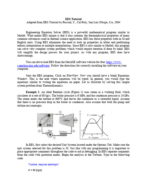
EES TutorialAdapted from EES Tutorial by Pascual, C., Cal Poly, San Luis Obispo, CA, 2004Engineering Equation Solver (EES) is a powerful mathematical program similar to Matlab. What makes EES unique is that it also contains the thermophysical properties of many common substances used in thermal science application. EES has these properties both in SI and English units. Using EES eliminates the need to look up properties in tables and performing tedious interpolation or multiple interpolations. Since EES is also similar to Matlab, this program can solve very complex system problems which would require iteration if done by hand. EES will simplify the design process for your project. As with any program, EES does have shortcomings.You can down load EES from the MechSE software website for free: https://www-/software/. Follow the directions for correctly installing the software on your computer.Start the EES program. Click on File>New. Now you should have a blank Equations Window. This is the area where equations will be typed. In general, you would type the equations similar to writing the equations on paper. Let us illustrate by solving this simple system problem from Thermodynamics.Example 1: An ideal Rankine cycle (Figure 1) uses steam as a working fluid, which circulates at a rate of 80 kg/s. The boiler pressure is 6 MPa, and the condenser pressure is 10 kPa. The steam enters the turbine at 600°C and leaves the condenser as a saturated liquid. Assume that there is no pressure drop in the boiler or condenser. Also assume that both the pump and turbine are isentropic.In EES, first select the desired Unit System located under the Options Tab. Make sure the unit system selected for this problem is SI. Just like with any programming it is important to place appropriate comments throughout the code to aid in debugging. In EES separate comments from the code with quotation marks. Begin the analysis at the Turbine. Type in the following code:"Turbine: Assume isentropic"m = 80 [kg/s]P_boiler = 6000 [kPa]T_3 = 600 [C]h_3 = enthalpy(steam, P=P_boiler, T=T_3)s_3 = entropy(steam, P=P_boiler, T=T_3)P_condenser = 10 [kPa]h_4 = enthalpy(steam, P=P_condenser, s=s_3)W_turbine = m*(h_3-h_4) "[kW]"EES has the ability to check units for you but conversion factors must be used and all variables must be assigned a unit. Above, by placing the units for the variables in brackets ([kPa]), you are assigning units to this variable. In the solution window, this unit will appear next to the variable. This type of assignment only works when a variable is assigned a numeric value like P_boiler. You will notice that next to W_turbine, the units are typed as "[kW]". In this situation, the units have not been assigned to the variable because EES does not know which variable in that equation has units of kW. Therefore, to properly assign units to W_turbine, highlight the variable W turbine and right click the mouse. Choose Variable Info. Enter units as kW.The underscore symbol (like h_4) is used to denote a subscript. Therefore, in the Formatted Equation window the variable h_4 will appear as h_4. Go to the Windows tab and select Formatted Equations. Another window will open showing the equations in a neat printable form.You do not have to remember the format for the property equations. Instead go to the Options tab and select Function Info. From here select Fluid Properties. The box on the left shows the property, while the box on the right shows the fluid. Instead of typing the equation, choose enthalpy and steam and then paste (Do not do this now since you already typed in the equation above). Remember from the State Postulate, that you need two independent properties to define the state. The function information shows pressure and temperature, but you can choose any two independent properties. In setting the enthalpy at state 4, notice that pressure and entropy were chosen. Now type the following code for the remainder of the system components."Condenser: Assume no pressure drop"h_1 = enthalpy(steam, P = P_condenser, x = 0) "Aside: Recall x is the quality"s_1 = entropy(steam, P =P_condenser, x = 0)Q_condenser = m*(h_1 - h_4) "[kW]""Pump: Assume isentropic"h_2 = enthalpy(steam, P= P_boiler, s = s_1)W_pump = m*(h_1 - h_2) "[kW]""Boiler: Assume no pressure drop"Q_boiler = m*(h_3-h_2) "[kW]""efficiency"eta = (W_turbine+W_pump)/Q_boiler "[-]"EES does not recognize the difference between lower and upper case letters; therefore, variables q and Q are interpreted as the same variable. Greek letters are entered by typing their full name like eta for 11. In the Formatted Equations, Greek letters appear as their symbol. Finally, has no units and that is indicated by [-] next to the variable. Don't forget to add units to Q_condenser, W_pump, Q_boiler, and eta.Now that the code has been entered, the system of equations can be solved. Before solving the equation, check for any syntax errors by clicking on Check/Format under the Calculate tab (or by pushing the red check button). If no errors are found, this check will inform you of the number of equations and the number of unknowns. If the number of equations and number of unknowns are not equal, no solution can be found. If the format is correct, then click on Solve also under the Calculate tab (or by clicking the calculator button). The solution window will appear showing the values for all the variables. EES will also perform a units check. Click Check Units under the Calculate tab. You will notice that the properties have units automatically added. The answers for the first exercise are: W turbine= 110990 kW, Q condenser= -166318 kW, W pump = -483.5 kW, Q boil =276825 kW, and 0.3992.Clicking Print under the File tab will print the program and solution. The formatted equations choice will print out the equations in a format similar to written equations. Another powerful feature of EES is the Parametric Table. This feature allows you to vary parameters and see the result on the system. This feature will be very useful in your design project when choosing the best overall design. This feature will be illustrated with the following example.Example 2: The condenser pressure from Example 1 is now allowed to vary from 2 kPa to 10 kPa. How does varying condenser pressure affect the power from the turbine and the efficiency of the cycle?Click on New Parametric Table under the Tables tab. For this example, choose 9 runs, and title the table as Condenser Pressure. The left box shows all the variables in the program. Choose P_condenser first. Click Add. Now P_condenser is removed from the left box and placed in the right box. Next addW_turbine and eta to the box on the right and click OK. A spreadsheet looking table now appears withP condenser, W turbine, and appearing at the top. On the column for P condenser, click on the black arrow at the top. Set the first value to 10 and the last value to 2 (therefore, the pressure will vary from 10 kPa to 2 kPa in 1 kPa increments) and click OK. EES will now fill in the column of P condenser with the test values. EESwill now solve the program for each value of P condenser and insert the corresponding values of W turbine and in the appropriate column. To solve the table either click the green arrow in the upper left or click Solve Table under the Calculate Tab. To avoid an error in solving the table, the equation, which sets the value for P condenser, must be deleted in the Equations window. Therefore there is one variable more than the number of equations.As the condenser pressure drops, the power from the turbine and the cycle efficiency increase. You can plot this trend by clicking New Plot Window (X-Y Plot) under the Plots tab. Choose P_condenser for the x-axis and W_turbine for the y-axis. Before clicking OK, check the automatic update box, so the graph will be updated every time the table is updated. The plot can be resized by dragging the lower right hand corner. Now add the efficiency data by clicking Overlay Plot under the Plots tab. Select eta for the y-axis and select Y2 for the right Y-scale. Don't forget to click automatic update before hitting OK. Your graph should look similar to Figure 2. If it doesn't look similar to Figure 2 then adjust the y-axis scales. There are many features which are similar to Excel, which allow you to change the format of the plot and addt ext. Now let us do another example, which is more difficult.Figure 3. Rankine Cycle with RegenerationExample 3: The ideal Rankine cycle described in Example 1 is modified to include the regeneration process. A portion of the steam is extracted from the high-pressure turbine at 0.5 MPa and is used to heat the feedwater in an open feedwater heater (Figure 3). The rest of the steam enters the condenser at 10 kPa. All other conditions are the same as Example I. You may assume that both pumps and the turbine are isentropic. The open feedwater heater is at saturation conditions with a pressure of 0.5 MPa. Here is the program to solve this example. Start with a new equation window."Turbine: Assume isentropic"m = 80 [kg/s]P_boiler = 6000 [kPa]T_5=600 [C]h_5 = enthalpy(steam, T = T_5,P = P_boiler)s_5 =entropy(steam, T= T_5, P= P_boiler)P_condenser = 10 [kPa]h_7 = enthalpy(steam, P = P_condenser, s = s_5)T_7 = temperature(steam, P = P_condenser, s = s_5)h_6 = enthalpy(steam, P = 500, s = s_5)m_7 = m - m_6 "Mass Balance"W_turbine = m*h_5 - m_6*h_6 - m_7*h_7 "[kW]""Condenser: Assume no pressure drop"h_1 = enthalpy(steam, P = P_condenser, x = 0)s_1 = entropy(steam, P = P_condenser, x = 0)Q_condenser = m_7*(h_1 -h_7) "[kW]""Low-Pressure Pump: Assume isentropic"h_2 = enthalpy(steam, P = 500, s = s_1)W_lowpump = m_7*(h_1 -h_2) "[kW]""Feedwater Heater: Assume saturated system"h_3 = enthalpy(steam, P = 500, x = 0) "Saturated liquid at exit of feedwater heater"s_3 = entropy(steam, P = 500, x = 0)m_6 = (m*h_3 -m_7*h_2)/h_6 "[kg/s]""High-Pressure Pump: Assume isentropic"h_4 = enthalpy(steam, P = P_boiler, s = s_3)W_highpump = m*(h_3 - h_4) "[kW]""Boiler: Assume no pressure drop"Q_boiler = m*(h_5 -h_4) "[kW]""Efficiency"eta = (W_turbine + W_lowpump + W_highpump)/Q_boiler "[-]"Don't forget to add units to the following variables: m_6, m_7, W_turbine, Q_condenser, W_lowpump, W_highpump, Q_boiler, and eta. After typing in the program, check the format and solve the equations. As you will see, the solution is solved iteratively since the mass flowrate to the feedwater heater was not known. However, EES was able to solve the problem. This is not always the case. Sometimes EES needs help. The next example will illustrate this point. The solution for Example 3 is: W turbine = 102581 kW, Q condenser = -138875 kW, W lowpump = -33 kW,W highpump = -480 kW, Q boiler = 240943 kW, = 0.4236.Example 4: A 25-mm diameter cable has an electrical resistance of 10-4 /m and istransmitting a current of 1000 A. If the cable is submerged in a tank of water at 1°C and is flowing at 5 m/s in cross flow over the cable, what is its surface temperature in °C?From Newton ’s Law of Cooling, the heat transfer from the cable per unit length is:)('T T h D q s . Solving for the surface temperature: h D q T T s '. The properties of thefluid need to be evaluated at the film temperature: )(5.0T T T s film . As you will learn in heat transfer, these types of problems require iteration on the fluid properties since the filmtemperature is unknown. EES now makes this part easier (almost). The Hilpert correlation is used to calculate the heat transfer coefficient from a heated cylinder. Here is the program to solve this example. Start with a new equation window."Heat Transfer Rate"q = 1000^2*10^(-4)"Heat Transfer Coefficient"T_0 = 10 [C]T_film = 0.5*(T_0+T_surf) "[C]"Nu = VISCOSITY(water, T=T_film, P=101.32)/DENSITY(Water, T=T_film, P=101.32)V = 5 [m/s]D = 0.025 [m]Re_D =V*D/nu "[-]"Pr = PRANDTL(Water, T=T_film, P=101.32)NuD = 0.193*Re_D^0.618*Pr^(1/3) "[-] Hilpert Correlation"k = CONDUCTIVITY(Water, T=T_film, P=101.32)h = NuD*k/D "[W/m^2-C]""Surface Temperature"T_surf = T_0 + q/(pi*h*D)After checking the format of the equations, adding units to variables and correcting any syntax errors, click calculate. More than likely, EES will give you some type of error, which does not result in a solution. This error is not a result of a programming mistake, but instead it is a mistake in your initial guesses. Click on Variable Info under the Options tab. This screen will show you all the variables, their initial guess, their lower limit, their upper limit, and their units. The default values are negative infinity for the lower limit, positive infinity for the upper limit, and an initial guess of 1. For this example, these particular limits and guess are not working so you need to change them. In order to come up with intelligent guesses, you need to know how the system is behaving. In this example not knowing the film temperature is causing the properties to be poorly guessed. Therefore replace the equation for the film temperature with T_film=10°C and solve the problem. Now you have a solution, which is not correct but it is better than no solution. Use this solution to update the guesses in the Variable Info window and resolve the problem by putting the original equation for T_film back into the program. The answers are T surf = 10.1 °C and T film = IO.06°C.。

ScalaTutorial-zh_CN

A Scala Tutorialfor Java programmersVersion1.3March15,2009Michel Schinz,PhilippHaller靳雄飞（中文翻译）P ROGRAMMING M ETHODS L ABORATORYEPFLS WITZERLAND1 介绍－ Introduction本文档是Scala语言和编译器的快速入门介绍，适合已经有一定编程经验，且希望了解Scala可以做什么的读者。

我们假定本文的读者具有面向对象编程（Object-oriented programming，尤其是java相关）的基础知识。

This document gives a quick introduction to the Scala language and compiler. Itis intended for people who already have some programming experience and wantan overview of what they can do with Scala. A basic knowledge of object-oriented programming, especially in Java, is assumed.2 第一个例子－A first example我们使用最经典的“Hello world”作为第一个例子，这个例子虽然并不是特别炫（fascinating），但它可以很好的展示Scala的用法，且无须涉及太多的语言特性。

示例代码如下：As a first example, we will use the standard Hello world program. It is not very fascinatingbut makes it easy to demonstrate the use of the Scala tools without knowing too much about the language. Here is how it looks:object HelloWorld { defmain(args: Array[String]){ println("Hello,world!") } }Java程序员应该对示例代码的结构感到很熟悉：它包含一个main方法，其参数是一个字符串数组，用来接收命令行参数；main的方法体只有一句话，调用预定义的println 方法输出“Hello world！”问候语。

Direct3D11Tutorial1：Basics_Direct3D11教程1：基础

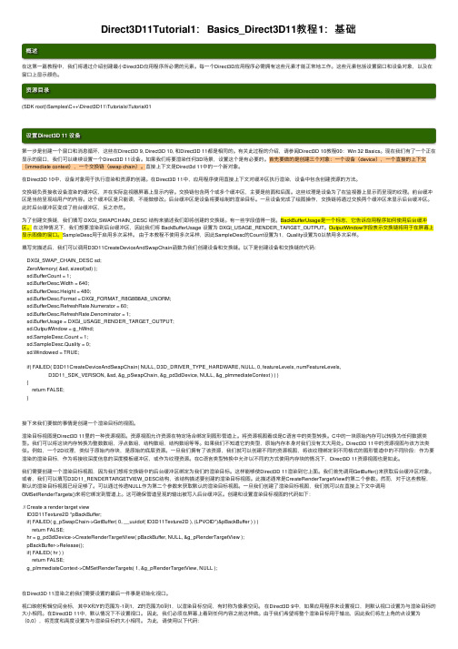
Direct3D11Tutorial1：Basics_Direct3D11教程1：基础概述在这第⼀篇教程中，我们将通过介绍创建最⼩Direct3D应⽤程序所必需的元素。

每⼀个Direct3D应⽤程序必需拥有这些元素才能正常地⼯作。

这些元素包括设置窗⼝和设备对象，以及在窗⼝上显⽰颜⾊。

资源⽬录(SDK root)\Samples\C++\Direct3D11\Tutorials\Tutorial01设置Direct3D 11 设备第⼀步是创建⼀个窗⼝和消息循环，这些在Direct3D 9, Direct3D 10, 和Direct3D 11都是相同的。

有关此过程的介绍，请参阅Direct3D 10教程00：Win 32 Basics。

现在我们有了⼀个正在显⽰的窗⼝，我们可以继续设置⼀个Direct3D 11设备。

如果我们将要渲染任何3D场景，设置这个是有必要的。

⾸先要做的是创建三个对象：⼀个设备（device），⼀个直接的上下⽂（immediate context），⼀个交换链（swap chain）。

直接上下⽂是Direct3d 11中的⼀个新对象。

在Direct3D 10中，设备对象⽤于执⾏渲染和资源的创建。

在Direct3D 11中，应⽤程序使⽤直接上下⽂对缓冲区执⾏渲染，设备中包含创建资源的⽅法。

交换链负责接收设备渲染的缓冲区，并在实际监视器屏幕上显⽰内容。

交换链包含两个或多个缓冲区，主要是前⾯和后⾯。

这些纹理是设备为了在监视器上显⽰⽽呈现的纹理。

前台缓冲区是当前呈现给⽤户的内容。

这个缓冲区是只能读，不能做修改。

后台缓冲区是设备将要绘制的渲染⽬标。

⼀旦设备完成了绘图操作，交换链将通过交换两个缓冲区来显⽰后台缓冲区。

此时后台缓冲区变成了前台缓冲区，反之亦然。

为了创建交换链，我们填写 DXGI_SWAPCHAIN_DESC 结构来描述我们即将创建的交换链。

有⼀些字段值得⼀提。

BackBufferUsage是⼀个标志，它告诉应⽤程序如何使⽤后台缓冲区。

Qt 教程

传智播客– C++学院Qt5教程目录目录 (1)1Qt概述 (3)1.1 什么是Qt (3)1.2 Qt的发展史 (4)1.3 支持的平台 (4)1.4 Qt版本 (4)1.5 Qt的安装 (5)Linux Host (5)OS X Host (5)Windows Host (5)1.6 Qt的优点 (5)2创建Qt项目 (6)2.1 使用向导创建 (6)2.2手动创建 (9)2.3.pro文件 (10)2.4一个最简单的Qt应用程序 (12)3信号和槽机制 (13)3.1 信号和槽 (13)3.2 自定义信号槽 (15)自定义信号槽需要注意的事项 (18)信号槽的更多用法 (18)3.3 Lambda表达式 (19)4 Qt窗口系统 (21)4.1 Qt窗口坐标体系 (21)坐标体系 (21)4.2 QWidget (21)4.3 QMainWindow (23)4.3.1 菜单栏 (24)4.3.2 工具栏 (25)4.3.3 状态栏 (25)4.4 资源文件 (26)4.5 对话框QDialog (29)4.5.1 基本概念 (29)4.5.2 标准对话框 (30)4.5.3 自定义消息框 (31)4.5.4 消息对话框 (33)4.5.5 标准文件对话框 (36)4.6 常用控件 (39)4.6.1 QLabel控件使用 (39)4.6.2 QLineEdit (41)4.6.3 其他控件 (43)4.7 布局管理器 (43)4.7.1 水平/垂直/网格布局 (44)4.7.2 自定义控件 (46)5 Qt消息机制和事件 (50)5.1 事件 (50)5.2 event（） (52)5.3 事件过滤器 (55)5.4 总结 (59)5.5 不规则窗体 (62)6 绘图和绘图设备 (63)6.1 QPainter (63)6.2 绘图设备 (65)6.2.1 QPixmap、QBitmap、QImage (65)6.2.2 QPicture (69)7 文件系统 (70)7.1 基本文件操作 (71)7.3 文本文件读写 (75)8 Socket通信 (76)8.1 TCP/IP (77)服务器端 (77)客户端 (79)8.2 UDP (81)广播 (82)组播 (82)8.3 TCP/IP 和UDP的区别 (83)9 多线程 (83)9.1 线程介绍 (84)9.2 多线程的使用 (87)9.3 使用线程绘图 (89)10 数据库操作 (91)10.1 数据库操作 (91)10.2 使用模型操作数据库 (97)查询操作 (97)插入操作 (98)更新操作 (99)删除操作 (100)10.3 可视化显示数据库数据 (100)11 Qt程序打包 (102)1Qt概述1.1 什么是QtQt是一个跨平台的C++图形用户界面应用程序框架。

matlab-tutorial_do_exercises

Training Course onPractical Applications on Climate Variability StudiesExercises, day 11) Read the netcdf file ‘skt.mon.mean.nc’ (skin temperature derived from NCEP, monthly mean values for the period 1948-2004). Select the Southern Ocean region (southward of 50°S) and save the skt sub-sample as well as the latitude and longitude information, in matlab format.2) Read the netcdf file ‘skt.mon.mean.nc’ and create El Niño 3 time series for the period 1970-1999 (El Niño 3 box is defined as 5°S-5°N, 210°E-270°E). Save the series in binary format.3) Read the netcdf file ‘skt.mon.mean.nc’, mask the continents using the land-sea mask‘lsmask.19294.nc’, select the first year and compute the SST global mean.4) Read the matlab files of skin temperature ‘skt.25x25.year.mat’ for the years 1980-1989. Calculate the annual mean value and save a matlab file with 10-annual mean values of the skt field. Exercises, day 25) Read the 30-yr time series of El Niño 3 (output from exercise 2) and plot the series. Perform a running average (3 month window) and plot the smoothed series.6) Study the following vectorizing loops:a) Vectorizing a double FOR loopb) Vectorizing code that finds the cumulative sum of a vector every fifth elementsc) Create a code that repeats a vector value when the following value is 07) Read the netcdf file ‘skt.mon.mean.nc’, mask the continents (using the land-sea mask‘lsmask.19294.nc’), estimate the annual mean SST value for 1948 and plot the map in different projections.8) Create scatter plots…Exercises, day 39) Read the netcdf zonal wind file ‘uwnd3.mon.mean.nc’. Select the period 1990-1999, estimate the mean and the standard deviation. i) Plot the maps at 1000 hPa; ii) Plot the zonal mean10) Read the 30-yr time series of El Niño 3 (output from exercise 2) and the slp files‘slp.25x25.year.mat’. Plot the correlation maps between El Niño 3 series and the SLP everywhere. Moreover, highlight only those regions where the correlations are significant (at 0.05). Repeat the exercise but filtering (high-pass, low-pass and band-pass filters).11) Read the SST HadISST dataset ‘SST_19821999.T42.grd’. Select the latitude of 56°S, calculate the anomalies band pass filtered, retaining interannual band 3-7yr of variability and plot the Hovmöller displaying the Antarctic Circumpolar Wave.12) Study two scripts for interpolation. In the first case, interpolation is done between two regular grids. In the second case, discretization of the output field is an irregular grid.13) Read the geopotential field ‘z500.25ond.grd’. The file contains the variable at 500 hPa, and time series is 25 years length (October-November-December mean values). Calculate the EOF in the global domain, from linear detrended anomalies. Plot the EOF-1, the PC-1 and save the output files in grd format.Exercises, day 414) The same as 13) but performing the EOFs in the southern extratropical domain (south of aprox 42°S) and saving the output files in netcdf format.15) The same as 14) but including a varimax rotation.16) The same as 13) but performing the EOFs of SST masking fields. Input data are‘sst.25x25.year.mat’.17) Study the script that performs a combined EOF (CEOF) analysis over the tropical Pacific region. Variables for the CEOF are SST, ORL, u(850 hPa) and v(850 hPa). Input dataset is‘ssta_olra_u-v850a_1979_2002.mat’.18) Perform the spectrum of El Niño 3 time series (output from exercise 2) using diverse methods(e.g., covariance method, Welch’s method).19) Study the script that performs a wavelet analysis of a long El Niño 3 time series ‘ninio3_1871-1999.grd’.20) Probability density function: an example of using interactive screens (pdftool).。

1、下载文档前请自行甄别文档内容的完整性，平台不提供额外的编辑、内容补充、找答案等附加服务。
2、"仅部分预览"的文档,不可在线预览部分如存在完整性等问题,可反馈申请退款(可完整预览的文档不适用该条件!)。
3、如文档侵犯您的权益，请联系客服反馈,我们会尽快为您处理(人工客服工作时间：9:00-18:30)。

But use instead:
./xcConfigure script
BEWARE: set XCRYSDEN_SCRATCH to something like: /scratch/$USER/xcrys_tmp
What xcConfigure does?
(1) defines: XCRYSDEN_TOPDIR and XCRYSDEN_SCRATCH
file. $HOME/.xcrysden/Xcrysden_defaults file.
$HOME/.xcrysden/custom-definitions
(4) asks several questions and writes answers in $HOME/.xcrysden/custom-definitions file.
PWgui
analyze by XCrySDen
pw.x < stdin > stdout output: prefix.*
●
calculate property:
PWgui
pp.x < stdin > stdout output: filplot
• filter (transform) the data:
XCRYSDEN as a crystal-structure viewer
• select menu: File->XCrySDen Examples ...->XSF Files • open file: ZnS.xsf • learn how to:
– modify number of displayed cells (Modify->Number of Units Drawn) – change the unit of repetition (Display->Unit of Repetition ...->) – display Wigner-Seitz cell (Display->Wigner-Seitz Cells) – display Brillouin zone (Tools->k-path Selection)
– cd /scratch/$USER/**** ( **** == your directory ) – wget /download/xc-latestlinuxPC-static.tar.gz – (or open web page ) – tar zxvf xc-latest-linuxPC-static.tar.gz
XCrySDen Installation
– Do the following: – cd XCrySDen-*bin-static/ – ./xcConfigure
( set XCRYSDEN_SCRATCH to /scratch/$USER/xcrys_tmp )
– for Csh: source ~/.cshrc; rehash
( Note: requires the whirlgif and mpeg_encode programs to be defined in ~/.xcrysden/custom-definitions )
●
●
●
●●Βιβλιοθήκη CRYSDEN & PWscf
• Visualization of structures from PW.X input file: – xcrysden --pwi input.file • Visualization of structures from PW.X output file: – xcrysden --pwo output.file
• Lighting-On mode:
– more fancy display with shades, not so fast, but displays all possible items !!!
• Message:
!!!for isosurfaces and alike use Lighting-On mode !!!
Scheme; (Modify->Number of Units Drawn) colors
select: Slab
Generic use of XCRYSDEN
–Q: I want to visualize the structure from XXX formated file with XCRYSDEN? –A: Write an XXX2xsf filter and convert your file to XSF format: – xxx2xsf < file.xxx > file.xsf – xcrysden --xsf file.xsf – XSF specification is available on:
PWgui
analyze by XCrySDen
pp.x < stdin > stdout output: fileout
About XCrySDen
XCrySDen is a crystalline and molecular structure visualisation program
XCrySDen = (X-window) Crystalline Structures and Densities
• remember!!!
– Display menu: toggles displays (on/off) – Modify menu: changes the appearance of displayed items
• open file: fcc-410-1x1.xsf
– display at least 44 unit cells – try: Tools->Color
environmental variables (writes either into ~/.bashrc, ~/.profile or ~/.cshrc)
(2) creates: XCRYSDEN_SCRATCH directory. (3) creates: $HOME/.xcrysden directory.
How to print (to file)
• • select menu: File->Print in the “Print to File” windows specify the name of the file. The format is selected by a given extension. For example: – file.png – will save PNG file – file.gif – will save GIF file – file.eps – will save EPS file – etc. • XCRYSDEN's print is a screen-dump therefore before printing (to file): – maximize XCRYSDEN's main window – zoom the structure as much as possible – increase the tessellation factor (Modify->Tessellation Factor) to approx. 40 to 50
Lighting On/Off display-mode
• VERY IMPORTANT !!!
– two levels of display modes:
• Lighting-Off mode:
– very fast, but can display only atoms and bonds !!!
http://[ESPRESSO-TUTORIAL-SITE]/tutorial_xcrysden.pdf
Basic scheme ...
prepare by PWgui
pw.x < stdin > stdout
analyze by XCrySDen
●
perform SCF calculation:
– (for Bash: source ~/.bashrc ) – then execute with: xcrysden
XCRYSDEN as a molecular viewer
• select menu: File->XCrySDen Examples ...->XSF Files • open file: 2.xsf • learn how to: – rotate, zoom, change display mode, ... – measure distances, angles, dihedrals, ... – modify various display parameters ... • learn the menus: – Display menu: toggles displays (on/off) – Modify menu: changes the appearance of displayed items
XCRYSDEN – a short tutorial –
Cagliari, September 2005
Guido Fratesi (mostly based on Anton Kokalj's work)
Copy me ...
• this tutorial can be downloaded from:
• Tools-->k-path Selection
– select a k-path by mouse-clicking – save the file with .pwscf extension (BEWARE: .pwscf extension is mandatory to get the pw.x formatted k-list)