ansoft Maxwell 涡流分析材料(英文)
(完整)ANSYS Maxwell涡流场分析案例
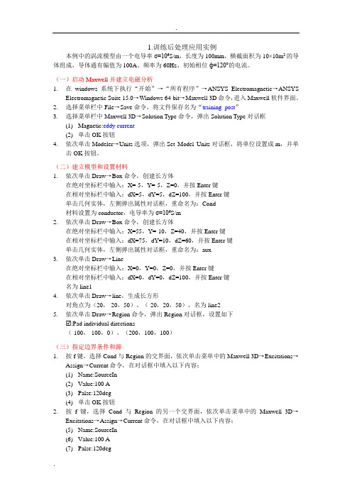
1.训练后处理应用实例本例中的涡流模型由一个电导率σ=106S/m,长度为100mm,横截面积为10×10m2的导体组成,导体通有幅值为100A、频率为60Hz、初始相位ф=120°的电流。
(一)启动M a x w e l l并建立电磁分析1.在windows系统下执行“开始”→“所有程序”→ANSYS Electromagnetic→ANSYS Electromagnetic Suite15.0→Windows 64—bit→Maxwell 3D命令,进入Maxwell软件界面。
2.选择菜单栏中File→Save命令,将文件保存名为“training_post”3.选择菜单栏中Maxwell 3D→Solution Type命令,弹出Solution Type对话框(1)Magnetic:eddy current(2)单击OK按钮4.依次单击Modeler→Units选项,弹出Set Model Units对话框,将单位设置成m,并单击OK按钮.(二)建立模型和设置材料1.依次单击Draw→Box命令,创建长方体在绝对坐标栏中输入:X=-5,Y=-5,Z=0,并按Enter键在相对坐标栏中输入:dX=5,dY=5,dZ=100,并按Enter键单击几何实体,左侧弹出属性对话框,重命名为:Cond材料设置为conductor,电导率为σ=106S/m2.依次单击Draw→Box命令,创建长方体在绝对坐标栏中输入:X=55,Y=-10,Z=40,并按Enter键在相对坐标栏中输入:dX=75,dY=10,dZ=60,并按Enter键单击几何实体,左侧弹出属性对话框,重命名为:aux3.依次单击Draw→Line在绝对坐标栏中输入:X=0,Y=0,Z=0,并按Enter键在相对坐标栏中输入:dX=0,dY=0,dZ=100,并按Enter键名为line14.依次单击Draw→line,生成长方形对角点为(20,—20,50)、(-20,20,50),名为line25.依次单击Draw→Region命令,弹出Region对话框,设置如下:Pad individual directions(—100,-100,0)、(200,100,100)(三)指定边界条件和源1.按f键,选择Cond与Region的交界面,依次单击菜单中的Maxwell 3D→Excitations→Assign→Current命令,在对话框中填入以下内容:(1)Name:SourceIn(2)Value:100 A(3)Palse:120deg(4)单击OK按钮2.按f键,选择Cond与Region的另一个交界面,依次单击菜单中的Maxwell 3D→Excitations→Assign→Current命令,在对话框中填入以下内容:(5)Name:SourceIn(6)Value:100 A(7)Palse:120deg(8)按Swap Direction和OK按钮(四)设置求解规则1.依次选择菜单栏中Maxwell 3D→Analysis Setup→Add Solution Setup命令,此时弹出Solution Setup对话框,在对话框中设置:(1) Maximum number of passes(最大迭代次数):10 (2) Percent Error (误差要求):1%(3) Refinement per Pass(每次迭代加密剖分单元比例):50% (4) Solver>Adaptive Frequency(设置激励源的频率):60Hz (5) 单击OK 按钮。
Maxwell 中英文对照资料讲解
辅绕组系数 主、副绕组相位差 互感漏抗
Aux.-Phase Winding Factor: Angle Btween Main & Aux.Winding Axes (degrees) Mutual Leakage Reactance(ohm):
定子齿磁通密度 Stator-Teeth Flux Density (Tesla):
Aux. Slot Leakage Reactance (ohm):
Aux. End-Winding Leakage Reactance (ohm):
Aux. Differential Leakage Reactance (ohm):
Rotor Slot Leakage Reactance (ohm):
副绕组电流
Aux.-Phase Current (A):
主、辅绕组相位电流 Phase Shift between Mainand Aux.
差
Currents (degrees):
电容电压
Capacitor Voltage (V):
电容损耗
Capacitor Loss (W):
定子绕组铜损耗 Copper Loss of Stator Winding (W):
风摩
Wind Loss (W):
负载类型
Type of Load:
铁心长度
Iron Core Length (mm):
铁心叠压系数
Stacking Factor of Iron Core:
硅钢片牌号
Type of Steel:
工作温度
Operating Temperature (C):
转子位置
Rotor Position:
(完整版)关于Ansoftmaxwell中电机铁耗和涡流损耗计算的说明

(完整版)关于Ansoftmaxwell中电机铁耗和涡流损耗计算的说明考虑到最近很多⼈在问这个问题,因此专门整理出来,供新⼿参考。
先谈⼀下什么情况下需要做铁耗分析。
对常规交流电机(同步或者异步电机),只有定⼦铁⼼才会产⽣铁耗,转⼦铁⼼是没有铁耗的,学过电机的⼈都明⽩的。
因此,只需要对定⼦铁⼼给出B-P曲线(也就是铁损曲线)。
注意,B-P 曲线分为单频和多频两种,能给出多频损耗曲线最好,这样maxwell算得准些。
设置完铁损曲线以后,还要记得在excitations/set core loss,对定⼦铁⼼勾选才⾏。
此时,不需要给定⼦和转⼦铁⼼再施加电导率,这是初学者容易忽视的问题。
后处理中,通过result/create transient reports/core loss查看铁耗随时间变化曲线。
再谈⼀下什么情况下需要做涡流损耗分析。
对永磁电机,永磁体受空间⾼次谐波的影响,会在表⾯产⽣涡流损耗;对实⼼转⼦电机,由于是⼤块导体,因此涡流损耗占绝⼤部分。
以上两种情况需要考虑做涡流损耗分析。
现以永磁电机为例,具体阐述。
对永磁体设置电导率,然后对每个永磁体分别施加零电流激励源,在excitations/set eddy effect,对永磁体勾选。
注意,若只考虑永磁体的涡流损耗,⽽不考虑电机其他部分(定转⼦铁⼼)的涡流损耗,则只需要给永磁体赋予电导率值,其他部件不需要赋电导率,这是初学者容易搞错的地⽅。
简⽽⾔之,只对需要考虑涡流损耗的部件,施加电导率,零电流激励和set eddy effect。
后处理中,通过results/create transient reports/retangular report/solid loss查看涡流损耗随时间变化曲线。
最后,再次强调⼀下,做涡流损耗分析,需要skin depth based refinement ⽹格剖分才⾏。
以上⽅法,适⽤于Ansoft maxwell 13.0.0及以上版本,并适⽤于所有电机种类。
ANSYSMaxwell涡流场分析案例教学内容
ANSYSMaxwell涡流场分析案例教学内容ANSYS Maxwell涡流场分析案例教学内容一、引言ANSYS Maxwell是一款强大的电磁场仿真软件,可以用于分析和优化电磁设备和系统。
其中,涡流场分析是ANSYS Maxwell的重要功能之一。
本文将介绍涡流场分析的基本原理和案例教学内容,帮助读者快速上手并应用于实际工程问题。
二、涡流场分析原理涡流场分析是基于安培定律和法拉第电磁感应定律的原理。
当导体材料中有变化的磁场时,会产生涡流。
涡流产生的原因是磁场的变化导致电场的环路产生感应电动势,从而在导体内部产生电流。
涡流的大小和分布情况与导体材料的电导率、磁场的强度和频率等因素有关。
三、案例教学内容1. 涡流场分析基本操作- 创建新项目:打开ANSYS Maxwell软件,点击“File”菜单,选择“New”,输入项目名称并选择适当的单位。
- 导入几何模型:点击“Geometry”菜单,选择“Import”选项,导入需要分析的几何模型文件。
- 定义材料属性:点击“Materials”菜单,选择“Assign/Edit Material Properties”选项,根据实际情况定义导体材料的电导率等属性。
- 设置边界条件:点击“Boundaries”菜单,选择“Assign/Edit Boundary Conditions”选项,设置边界条件,如电流密度、电压等。
- 运行仿真:点击“Solve”菜单,选择“Analyze All”选项,运行涡流场仿真。
- 结果分析:点击“Results”菜单,选择“Postprocess”选项,查看涡流场分布情况,并进行必要的后处理操作。
2. 涡流场分析案例- 案例1:电感器的涡流损耗分析在电感器中,由于交流电磁场的存在,会产生涡流损耗。
通过对电感器进行涡流场分析,可以评估涡流损耗的大小,并优化电感器的设计。
具体步骤如下:1) 导入电感器的几何模型。
2) 定义电感器材料的电导率。
Ansoft Maxwell简介与电场仿真实例PPT精选文档

4.设置计算参数(可选)
计算电容值:Maxwell 3D> Parameters > Assign > Matrix
计算参数
Force,力(虚位移法) Torque,转矩 Matrix,矩阵参数(对于静电场问题:部分电容参数矩阵)
静电独立系统— D 线从这个系统中的带电体发出,并终止于该系统 中的其余带电体,与外界无任何联系,即系统中,总净电荷为0。
12
继续建模:绘制外层屏蔽层模型 从Outer模型中减去Air模型,得到外层屏蔽层模型。 选中Outer模型和Air模型: Edit > Select > By Name
Shift+鼠标左键
13
继续建模:绘制外层屏蔽层模型 从Outer模型中减去Air模型,得到外层屏蔽层模型。
Modeler > Boolean > Subtract
双击
双击改名:Inner
单击改模型颜色
单击设置材料 :copper
11
继续建模:绘制外层屏蔽层模型 选中已建立的Inner模型,Ctrl+C, Ctrl+V
建立第2个圆柱体,命名为Outer,材料:Copper
双击修改模型尺寸 同理,建立第3个圆柱体,半径改为1mm,命名为Air,材料:vacuum 从Outer模型中减去Air模型,得到外层屏蔽层模型。
瞬态场(Transient Field)
用于求解某些涉及到运动和任意波形的电压、电流源激励的设 备。该模块能同时求解磁场、电路及运动等强耦合的方程,因 而可轻而易举地解决上述装置的性能分析问题。
4
Ansoft仿真步骤
选择求解器类型 建模
设置材料属性(电 导率,介电常数, 磁导率等)
ANSYSMawell涡流场分析案例

ANSYSMawell涡流场分析案例ANSYS Maxwell涡流场分析案例涡流场分析是一种基于涡流现象的电磁场分析方法,广泛应用于电机、变压器、感应加热等电磁设备的设计和优化。
ANSYS Maxwell是一款专业的电磁场仿真软件,可以进行涡流场分析,并提供详尽的结果和分析。
在本案例中,我们将以一个感应加热器为例,介绍如何使用ANSYS Maxwell进行涡流场分析。
感应加热器是一种利用涡流效应产生热能的设备,常用于金属加热、热处理等工业领域。
首先,我们需要准备感应加热器的几何模型。
可以使用ANSYS DesignModeler或其他CAD软件进行建模,将感应加热器的几何形状导入到ANSYS Maxwell中。
接下来,我们需要定义材料属性。
对于感应加热器的材料,一般使用导电材料,如铜、铝等。
在ANSYS Maxwell中,我们可以选择相应的材料模型,并设置导电率等材料属性。
然后,我们需要定义边界条件。
感应加热器一般通过电感耦合的方式产生涡流,因此我们需要在感应加热器表面施加电压或电流边界条件。
根据具体情况,我们可以选择施加恒定电压或电流,或者根据时间变化的电压或电流进行仿真。
完成几何模型、材料属性和边界条件的定义后,我们可以进行网格划分。
ANSYS Maxwell提供了多种网格划分算法和参数设置,可以根据需要选择合适的方法进行网格划分。
通常情况下,我们需要保证网格密度足够细致,以准确捕捉涡流场的细节。
完成网格划分后,我们可以进行涡流场分析。
在ANSYS Maxwell中,我们可以选择求解器和设置求解参数。
对于涡流场分析,一般使用瞬态求解器,并设置仿真的时间范围和时间步长。
根据具体情况,我们还可以设置其他参数,如收敛准则、求解精度等。
在求解过程中,ANSYS Maxwell将根据边界条件和材料属性计算涡流场的分布。
求解完成后,我们可以查看涡流场的结果,并进行后处理分析。
ANSYS Maxwell提供了丰富的后处理工具,可以绘制涡流场的矢量图、剖面图、动画等,以及计算涡流场的各种参数,如涡流损耗、感应电流等。
基于AnsoftMaxwell3D涡流场的铜排仿真分析
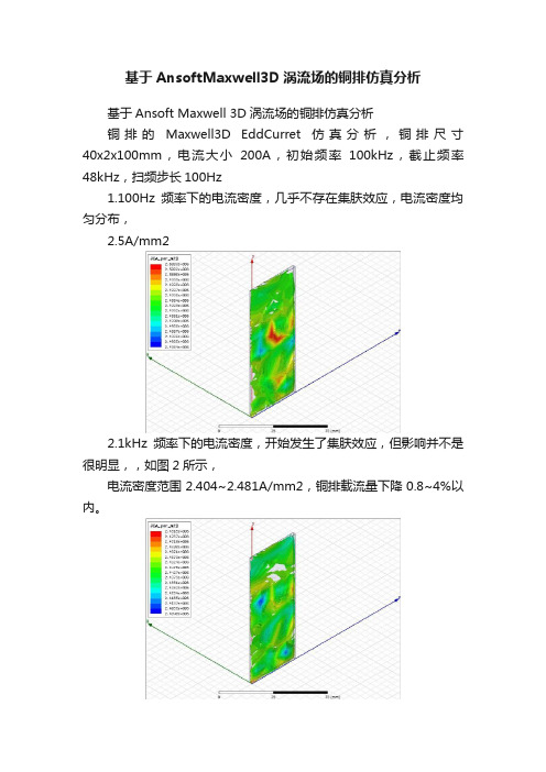
基于AnsoftMaxwell3D涡流场的铜排仿真分析基于Ansoft Maxwell 3D涡流场的铜排仿真分析铜排的Maxwell3D EddCurret仿真分析,铜排尺寸40x2x100mm,电流大小200A,初始频率100kHz,截止频率48kHz,扫频步长100Hz1.100Hz频率下的电流密度,几乎不存在集肤效应,电流密度均匀分布,2.5A/mm22.1kHz频率下的电流密度,开始发生了集肤效应,但影响并不是很明显,,如图2所示,电流密度范围2.404~2.481A/mm2,铜排载流量下降0.8~4%以内。
3. 1.5kHz频率下的电流密度,开始发生了集肤效应增加,但影响并不是很明显,如图2所示,电流密度范围2.32~2.44A/mm2,铜排载流量下降0.4~7.2%以内。
4. 2.5kHz频率下的电流密度,开始发生了集肤效应增加,影响很明显,如图2所示,电流密度范围2.09~2.34A/mm2,铜排载流量下降6.4~16.4%以内。
5.12kHz频率下的电流密度,很明显发生了集肤效应,电流密度均匀分布,如图2所示,电流密度范围0.325~1.07A/mm2,很明显铜排的载流量下降6.24kHz频率下的电流密度,很明显发生了集肤效应,电流密度均匀分布,如图2所示,电流密度范围0.019 ~0.506A/mm2,铜排的载流量进一步下降7.48kHz频率下的电流密度,很明显发生了集肤效应,电流密度均匀分布,如图2所示,电流密度范围0.0078 ~0.173A/mm2,铜排的载流量进一步下降分析与结论在大功率电力电子应用中,不仅仅核心的功率半导体器件需要严格的散热分析和设计,另外,交直流铜排也需要进行一定散热分析和处理,但其要求远远低于功率半导体器件。
A.SVG交流侧铜排:基本上输出的是基波电流,即50Hz的工频电流,另有含量非常低的谐波电流(一般谐波电流畸变率THD<3%)和开关纹波电流(占总电流5%左右)。
ANSYSMaxwell涡流场分析案例
1.训练后处理应用实例本例中的涡流模型由一个电导率σ=106S/m,长度为100mm,横截面积为10×10m2的导体组成,导体通有幅值为100A、频率为60Hz、初始相位ф=120°的电流。
(一)启动M a x w e l l并建立电磁分析1.在windows系统下执行“开始”→“所有程序”→ANSYS Electromagnetic→ANSYSElectromagnetic Suite 15.0→Windows 64-bit→Maxwell 3D命令,进入Maxwell软件界面。
2.选择菜单栏中File→Save命令,将文件保存名为“training_post”3.选择菜单栏中Maxwell 3D→Solution Type命令,弹出Solution Type对话框(1)Magnetic:eddy current(2)单击OK按钮4.依次单击Modeler→Units选项,弹出Set Model Units对话框,将单位设置成m,并单击OK按钮。
(二)建立模型和设置材料1.依次单击Draw→Box命令,创建长方体在绝对坐标栏中输入:X=-5,Y=-5,Z=0,并按Enter键在相对坐标栏中输入:dX=5,dY=5,dZ=100,并按Enter键单击几何实体,左侧弹出属性对话框,重命名为:Cond材料设置为conductor,电导率为σ=106S/m2.依次单击Draw→Box命令,创建长方体在绝对坐标栏中输入:X=55,Y=-10,Z=40,并按Enter键在相对坐标栏中输入:dX=75,dY=10,dZ=60,并按Enter键单击几何实体,左侧弹出属性对话框,重命名为:aux3.依次单击Draw→Line在绝对坐标栏中输入:X=0,Y=0,Z=0,并按Enter键在相对坐标栏中输入:dX=0,dY=0,dZ=100,并按Enter键名为line14.依次单击Draw→line,生成长方形对角点为(20,-20,50)、(-20,20,50),名为line25.依次单击Draw→Region命令,弹出Region对话框,设置如下:Pad individual directions(-100,-100,0)、(200,100,100)(三)指定边界条件和源1.按f键,选择Cond与Region的交界面,依次单击菜单中的Maxwell 3D→Excitations→Assign→Current命令,在对话框中填入以下内容:(1)Name:SourceIn(2)Value:100 A(3)Palse:120deg(4)单击OK按钮2.按f键,选择Cond与Region的另一个交界面,依次单击菜单中的Maxwell 3D→Excitations→Assign→Current命令,在对话框中填入以下内容:(5)Name:SourceIn(6)Value:100 A(7)Palse:120deg(8) 按Swap Direction 和OK 按钮(四)设置求解规则1. 依次选择菜单栏中Maxwell 3D →Analysis Setup →Add Solution Setup 命令,此时弹出Solution Setup 对话框,在对话框中设置:(1) Maximum number of passes (最大迭代次数):10(2) Percent Error (误差要求):1%(3) Refinement per Pass (每次迭代加密剖分单元比例):50%(4) Solver>Adaptive Frequency (设置激励源的频率):60Hz(5) 单击OK 按钮。
ANSYSMaxwell涡流场分析案例教学内容

ANSYSMaxwell涡流场分析案例教学内容ANSYS Maxwell涡流场分析案例教学内容涡流场分析是工程领域中一项重要的技术,可以用来研究电磁场中的涡流现象。
ANSYS Maxwell是一款强大的电磁场仿真软件,提供了丰富的工具和功能,用于分析和优化电磁设备和系统。
在本文中,我们将介绍一些ANSYS Maxwell涡流场分析的案例教学内容。
1. 涡流场分析基础在进行涡流场分析之前,首先需要了解涡流场的基本概念和原理。
涡流场是指当导体材料被交变电磁场穿过时,由于电磁感应作用而产生的涡流现象。
涡流会产生额外的能量损耗和热量,对电磁设备的性能和效率有重要影响。
因此,通过涡流场分析可以评估和改进电磁设备的设计。
2. 涡流场分析建模在进行涡流场分析之前,需要对电磁设备进行建模。
ANSYS Maxwell提供了多种建模工具,可以根据实际情况选择合适的建模方法。
例如,可以使用几何建模工具创建三维模型,或者使用参数化建模工具进行参数化建模。
建模过程中需要考虑材料的电磁特性和几何形状对涡流场的影响。
3. 涡流场分析设置在进行涡流场分析之前,需要设置分析的参数和条件。
ANSYS Maxwell提供了丰富的分析设置选项,可以根据实际需求进行设置。
例如,可以设置交变电磁场的频率、幅值和相位,以及材料的电导率和磁导率等参数。
通过合理设置分析参数,可以获得准确的涡流场分析结果。
4. 涡流场分析结果在进行涡流场分析之后,可以获得涡流场的分析结果。
ANSYS Maxwell提供了多种结果输出选项,可以直观地显示涡流场的分布和特性。
例如,可以显示涡流密度、涡流功率损耗和涡流温度等参数。
通过分析结果,可以评估电磁设备的性能和效率,并进行优化设计。
5. 涡流场分析案例下面我们将介绍几个涡流场分析的案例,以帮助读者更好地理解和应用ANSYS Maxwell软件。
案例一:涡流制动器设计涡流制动器是一种常用的制动装置,通过涡流场的产生和作用来实现制动效果。
S017-Ansoft HFSS系列经典培训教材-ANSOFT HFSS培训教材系列2(英文)

smart software for high-frequency design
2-7
HFSS Analysis Design Flow
Executive Window ‘checklist’ reflects 3 stages of Project design flow
s
PRE-PROCESSING
s
s
Modeled Geometry (interior air)
Therefore, Geometry must include all volumes in which E- and H- fields will exist Metals may be treated as surface conditions only; thickness need not be modeled if penetration is negligible effect (thickness > skin depth)
s
s s
This is intentional, to preserve the configuration from which any solution was derived. Editing a project’s setup files may delete meshes and solutions! To create a variation of an existing solved project, copy the original, and work on the copy!
Solution Monitoring Window
NOTE: All 3D Display windows in HFSS will have a BLACK background. This is not currently editable in HFSS Version 7. Graphical window images have been inverted for this and all subsequent training presentations for better paper reproduction.
最新Ansoft-Maxwell简介与电场仿真实例课件PPT

Ansoft Maxwell
Ansoft公司的Maxwell 是一个功能强大、结果精确、易于使用的二 维/三维电磁场有限元分析软件。包括静电场、静磁场、时变电 场,时变磁场,涡流场、瞬态场和温度场计算等,可以用来分 析电机、传感器、变压器、永磁设备、激励器等电磁装置的静 态、稳态、瞬态、正常工况和故障工况的特性。
Ansoft的自适应有限元计算
迭代停止条件:两种条件
1. Maximum number of passes
最大允许迭代次数
2.Percent error(设定误差) Energy Error和Delta Energy都要小于 Percent error
两种条件满足其一,计算停止
加密剖分原则:
将具有更高能量误差的 单元进行加密
• 刺营出血流派是指善用刺营出血
疗法来治疗疾病的医学家所形成 的学术派别。
二、学术发展过程
起源与萌芽阶段(春秋以前) 理论奠基阶段(内经时代) 经验积累阶段(隋唐时期) 理论创新及特色形成阶段(宋金元时期) 成熟阶段(明清时期) 空前发展阶段(近现代时期)
1、起源与萌芽阶段(春秋以前)
部分电容
Capacitance Matrix 部分电容矩阵
4导体静电独立系统 Q1C10V1C12(V1V2)C13(V1V3) Q2 C20V2C21(V2V1)C23(V2V3) Q3 C30V3C31(V3V1)C32(V3V2)
Q 1 C 10C 12C 13 C 12
Q 2 C 12
继续建模:绘制外层屏蔽层模型 从Outer模型中减去Air模型,得到外层屏蔽层模型。 选中Outer模型和Air模型: Edit > Select > By Name
maxwell材料库中英文对照
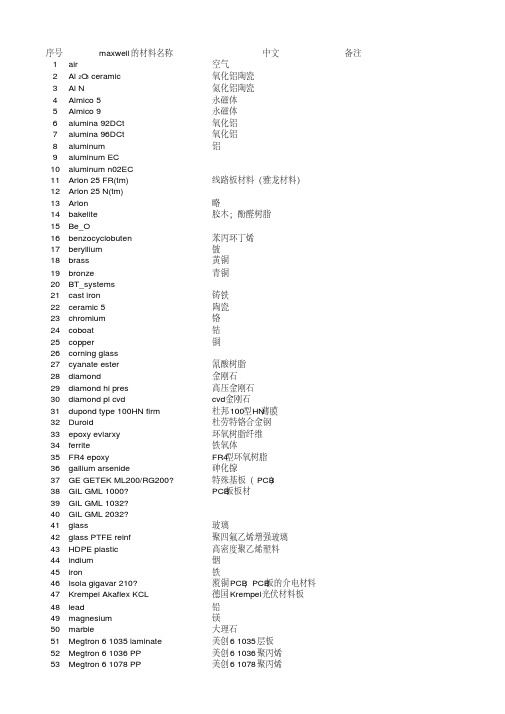
序号maxwell的材料名称中文备注1air空气2Al2O3 ceramic氧化铝陶瓷3Al N氮化铝陶瓷4Almico 5永磁体5Almico 9永磁体6alumina 92DCt氧化铝7alumina 96DCt氧化铝8aluminum铝9aluminum EC10aluminum n02EC11Arlon 25 FR(tm)线路板材料(雅龙材料)12Arlon 25 N(tm)13Arlon略14bakelite胶木;酚醛树脂15Be_O16benzocyclobuten苯丙环丁烯17beryllium铍18brass黄铜19bronze青铜20BT_systems21cast iron铸铁22ceramic 5陶瓷23chromium铬24coboat钴25copper铜26corning glass27cyanate ester氰酸树脂28diamond金刚石29diamond hi pres高压金刚石30diamond pl cvd cvd金刚石31dupond type 100HN firm杜邦100型HN薄膜32Duroid杜劳特铬合金钢33epoxy evlarxy环氧树脂纤维34ferrite铁氧体35FR4 epoxy FR4型环氧树脂36gallium arsenide砷化镓37GE GETEK ML200/RG200?特殊基板(PCB)38GIL GML 1000?PCB板板材39GIL GML 1032?40GIL GML 2032?41glass玻璃42glass PTFE reinf聚四氟乙烯增强玻璃43HDPE plastic高密度聚乙烯塑料44indium铟45iron铁46Isola gigavar 210?覆铜PCB;PCB板的介电材料47Krempel Akaflex KCL德国Krempel光伏材料板48lead铅49magnesium镁50marble大理石51Megtron 6 1035 laminate美创6 1035层板52Megtron 6 1036 PP美创6 1036聚丙烯53Megtron 6 1078 PP美创6 1078聚丙烯54Megtron 6 3313 laminate美创6 3313层板55mica云母56modified epoxy改进环氧树脂57molybdenum钼58mu metal镍铁高导磁合金59NdFe30钕铁硼3060NdFe35钕铁硼3561Nelco N4000-13?一种PCB无铅焊层压板材62Nelco N4000-13 SI63Neltec NH9294?一种高频PCB线路板材料64nickel镍65palladium钯66pec印刷电路、光电管67perfect conductor理想导体68platinum铂69plexiglass有机玻璃70polyamide聚酰胺(尼龙)71polyester聚酯(涤纶)72polyethylene聚乙烯73Polyflon copper-clad LILTEM覆铜74Polyflon cuFlon75Polyflon polyguide76Polyflon Nor CLAD77polyimide聚酰亚胺78polyimide Quartz聚酰亚胺石英79polystyrene聚苯乙烯80porcelain瓷器81PVC plastic聚氯乙烯塑料82quartz glass石英玻璃83rhodium铑84Rogers Ro 3003?罗杰斯Ro 3003覆铜板85rubber hard硬橡胶86sapphire蓝宝石87sheldahl Cornclad HF一种微波板材88silicon硅89silicon dioxide二氧化硅90silicon nitrade硅硝酸盐91silver银92sm co 24钐钴永磁体93sm co 28钐钴永磁体94solder焊料、焊锡95soldermask绿漆(PCB专用语)96steel 1008冷镦钢,08钢97steel 101010钢98steel stainless不锈钢99Taconic CER-10?高频线路板100tatalum钽101tatalum nitride氮化钽102Teflon聚四氟乙烯103Teflon based聚四氟乙烯基104tin锡105titanium钛106tungsten钨107vaccum真空108water distilled蒸馏水109water fresh淡水110water sea海水111ZEONEX RS420光学玻璃112ZEONEX RS420-LDS113zinc锌,锌合金114zirconium锆。
3 Ansoft Maxwell简介

1. Maximum number of passes
最大允许迭代次数
2.Percent error(设定误差) Energy Error和Delta Energy都要小于 Percent error
两种条件满足其一,计算停止
加密剖分原则:
将具有更高能量误差的 单元进行加密
Capacitance Matrix 部分电容矩阵
4导体静电独立系统 Q1 = C10V1 + C12 (V1 − V2 ) + C13 (V1 − V3 )
Q2 = C 20V2 + C 21 (V2 − V1 ) + C 23 (V2 − V3 ) Q3 = C30V3 + C31 (V3 − V1 ) + C32 (V3 − V2 )
3. Geometry> All objects
4. Domain
导出电场强度E 的数据 5. Export 数据保存路径:英文目录 可用写字板打开
导出电场强度E 的数据
Grid Output Min: [-0.002 -0.002 0] Max: [0.002 0.002 0.001] Grid Size: [0.0001 0.0001 0.001] Vector data "Domain(Volume(AllObjects), <Ex,Ey,Ez>)“
-2.0000000000000000e-003 -2.0000000000000000e-003 0.0000000000000000e+000 -2.6696090154630286e+002 -3.6309353467063706e+003 -1.9492643644693467e+002 ………
Ansoft Maxvell电磁仿真软件的应用实验报告

Ansoft Maxwell电磁仿真软件的应用实验报告一Maxwell 简介Ansoft公司的Maxwell是一个功能强大、结果精确、易于使用的二维/三维电磁场有限元分析软件。
包括静电场、静磁场、时变电场、涡流场、瞬态场和温度场计算等,可以用来分析电机、传感器、变压器、永磁设备、激励器等电磁装置的静态、稳态、瞬态、正常工况和故障工况的特性。
Maxwell还可以产生高精度的等效电路模型以供Ansoft的SIMPLORER模块和其他电路分析工具调用。
三维静电场分析(3D Electrostatic Field)用于分析由静止电荷、直流电压引起的静电场。
该模块直接计算标量电位,得到电场强度(E),电位移矢量(D),电场力、电场能量、转矩、电容值等。
可用于分析直流高压绝缘问题,电容器储能问题等。
三维直流磁场分析(3D DC Magnetic)用于分析由恒定电流、永磁体及外部激磁引起的磁场。
该模块可计算磁场强度(H),电流密度(J),磁感应强度(B),磁场力、磁场能量、转矩、电感等。
可用于分析直流载流线圈磁场,永磁体产生磁场等。
涡流场分析(Eddy Current Field)用于分析受涡流、集肤效应、邻近效应影响的系统。
它求解的频率范围可以从0到数百兆赫兹,能够计算损耗、铁损、力、转矩、电感与储能。
可用于分析导体中的涡流分布。
三维正弦电磁场特性等。
瞬态场(Transient Field)用于求解某些涉及到运动和任意波形的电压、电流源激励的设备。
该模块能同时求解磁场、电路及运动等强耦合的方程,因而可轻而易举地解决上述装置的性能分析问题。
二Maxwell 仿真步骤1 选择求解器类型2 建模3 设置材料属性(电导率,介电常数,磁导率等)4 设置激励源和边界条件5 自适应网格剖分6 有限元计算7 后处理三Maxwell仿真实例题目三:静电除尘器电磁场分析要求:掌握静电除尘的工作原理,建立静电除尘器模型,观测内部电场及能量的分布情况,并对结果进行分析。
ansoft maxwell

ansoft maxwellAnsoft Maxwell: A Comprehensive OverviewIntroductionAnsoft Maxwell is a powerful electromagnetic field simulation software package developed by Ansys. It offers engineers and designers the capability to accurately model and analyze electromagnetic phenomena, such as magnetic fields, electric fields, and electromagnetic devices. This document will provide a comprehensive overview of Ansoft Maxwell, including its features, applications, and benefits.Features of Ansoft MaxwellAnsoft Maxwell is equipped with a range of features that enable users to perform complex electromagnetic simulations efficiently. Some of its key features include:1. Finite Element Method (FEM) Solver: Ansoft Maxwell utilizes the finite element method to solve complex electromagnetic problems. This solver allows users toaccurately model and analyze the behavior of electromagnetic fields in various scenarios.2. 3D Modeling and Analysis: The software provides a robust 3D modeling environment that enables users to create intricate geometries and simulate electromagnetic fields in three dimensions. This feature is particularly useful for designing and optimizing complex electromagnetic devices and systems.3. Multi-Physics Simulations: Ansoft Maxwell allows for the integration of various physics phenomena into one simulation. This enables engineers to analyze the interaction between electromagnetic fields and other physical phenomena, such as structural mechanics or thermal effects.4. Material Database: The software includes a comprehensive material database that contains a wide range of electromagnetic properties for various materials. Users can easily select and assign appropriate material properties to their model, ensuring accurate and realistic simulations.5. Post-Processing and Visualization: Ansoft Maxwell offers advanced post-processing tools that allow users to visualize and analyze simulation results. Users can generate contourplots, vector plots, animations, and other visualization tools to gain insights into the behavior of electromagnetic fields.Applications of Ansoft MaxwellAnsoft Maxwell finds applications in various industries and engineering domains. Some of its common applications include:1. Electric Machine Design: Ansoft Maxwell is extensively used for designing and optimizing electric machines, such as motors, generators, and transformers. Engineers can analyze the electromagnetic performance of these machines, optimize their geometries, and enhance their efficiency using the software.2. High-Frequency Electronics: The software is widely used in the design and analysis of high-frequency electronic circuits and devices. Engineers can simulate the electromagnetic behavior of printed circuit boards (PCBs), antennas, microwave components, and other high-frequency systems.3. Power Electronics: Ansoft Maxwell plays a crucial role in the design and analysis of power electronic devices, such asinverters, converters, and power supplies. Engineers can analyze the electromagnetic behavior of these devices, optimize their designs, and ensure their reliable operation.4. Electromagnetic Compatibility (EMC) Analysis: Ansoft Maxwell enables engineers to perform electromagnetic compatibility analysis to ensure that electronic systems and devices do not interfere with each other or suffer from external electromagnetic interference. It allows for the identification and mitigation of potential interference issues.Benefits of Ansoft MaxwellThe use of Ansoft Maxwell provides several benefits to engineers and designers. Some of these benefits include:1. Accurate and Reliable Results: The software employs advanced numerical algorithms and solution techniques, ensuring accurate and reliable simulation results. Engineers can rely on the software's capabilities to make informed design decisions.2. Time and Cost Savings: Ansoft Maxwell enables engineers to rapidly iterate through design changes and evaluatemultiple design alternatives virtually. This accelerates the design process, reduces the need for physical prototypes, and ultimately saves time and cost.3. Improved Product Performance: By accurately analyzing electromagnetic behavior, engineers can optimize their designs to achieve improved product performance. This includes enhancing efficiency, reducing unwanted electromagnetic emissions, and minimizing electromagnetic susceptibility.4. Increased Design Confidence: Ansoft Maxwell provides engineers with a deeper understanding of the electromagnetic behavior of their designs. This increased insight instills confidence in the final design, as engineers can identify and address any potential issues before fabrication and testing.ConclusionAnsoft Maxwell is a comprehensive electromagnetic simulation software package that offers engineers and designers a range of powerful features, applications, and benefits. With its advanced capabilities and user-friendly interface, it enables the accurate modeling and analysis ofelectromagnetic fields in diverse scenarios. From electric machine design to high-frequency electronics and power electronics, Ansoft Maxwell serves as a valuable tool for numerous engineering disciplines. By utilizing this software, engineers can enhance product performance, improve design confidence, and achieve significant time and cost savings in their projects.。
- 1、下载文档前请自行甄别文档内容的完整性,平台不提供额外的编辑、内容补充、找答案等附加服务。
- 2、"仅部分预览"的文档,不可在线预览部分如存在完整性等问题,可反馈申请退款(可完整预览的文档不适用该条件!)。
- 3、如文档侵犯您的权益,请联系客服反馈,我们会尽快为您处理(人工客服工作时间:9:00-18:30)。
Chapter 6.0 Chapter 6.0 –Eddy Current Examples6.1 –Asymmetrical Conductor with a HoleExample (Eddy Current) –Asymmetrical ConductorThe Asymmetrical Conductor with a HoleThis example is intended to show you how to create and analyze anAsymmetrical Conductor with a Hole using the Eddy Current solver in the Ansoft Maxwell 3D Design Environment.Coil (Copper)Stock (Aluminum)Example (Eddy Current) –Asymmetrical Conductor Getting StartedLaunching Ansoft Maxwell1.To access Ansoft Maxwell, click the Microsoft Start button, select Programs, andselect the Ansoft > Maxwell 11program group. Maxwell 11.Setting Tool OptionsTo set the tool options:Note: In order to follow the steps outlined in this example, verify that thefollowing tool options are set:1.Select the menu item Tools > Options > Maxwell Options2.Maxwell Options Window:1.Click the General Options tabUse Wizards for data entry when creating new boundaries: ;CheckedDuplicate boundaries with geometry: ;Checked2.Click the OK button3.Select the menu item Tools > Options > 3D Modeler Options.4.3D Modeler Options Window:1.Click the Operation tabAutomatically cover closed polylines: ;Checked2.Click the Drawing tabEdit property of new primitives: ;Checked3.Click the OK buttonExample (Eddy Current) –Asymmetrical Conductor Opening a New ProjectTo open a new project:In an Ansoft Maxwell window, click the On the Standard toolbar, orselect the menu item File > New.From the Project menu, select Insert Maxwell Design.Set Solution TypeTo set the solution type:Select the menu item Maxwell > Solution TypeSolution Type Window:Choose Eddy CurrentClick the OK buttonExample (Eddy Current) –Asymmetrical Conductor Creating the 3D ModelSet Model UnitsTo set the units:1.Select the menu item 3D Modeler > Units2.Set Model Units:1.Select Units: mm2.Click the OK buttonSet Default MaterialTo set the default material:ing the 3D Modeler Materials toolbar, choose Select2.Select Definition Window:1.Type aluminum in the Search by Name field2.Click the OK buttonExample (Eddy Current) –Asymmetrical Conductor Create StockTo create the stock:1.Select the menu item Draw > Boxing the coordinate entry fields, enter the box positionX: 0.0, Y: 0.0, Z: 0.0, Press the Enter keying the coordinate entry fields, enter the opposite corner of the box:dX: 294.0, dY: 294.0, dZ: 19.0, Press the Enter key To set the name:1.Select the Attribute tab from the Properties window.2.For the Value of Name type: stock3.Click the OK buttonTo fit the view:1.Select the menu item View > Fit All > Active View.Create Hole in StockTo create the hole:1.Select the menu item Draw > Boxing the coordinate entry fields, enter the box positionX: 18.0, Y: 18.0, Z: 0.0, Press the Enter keying the coordinate entry fields, enter the opposite corner of the box:dX: 126.0, dY: 126.0, dZ: 19.0, Press the Enter key To set the name:1.Select the Attribute tab from the Properties window.2.For the Value of Name type: hole3.Click the OK buttonTo select the objects:1.Select the menu item Edit > Select AllTo complete the stock:1.Select the menu item 3D Modeler > Boolean > Subtract2.Subtract WindowBlank Parts: stockTool Parts: holeClick the OK buttonExample (Eddy Current) –Asymmetrical ConductorSet Default Materialing the 3D Modeler Materials toolbar, choose Select2.Select Definition Window:1.Type copper in the Search by Name field2.Click the OK buttonCreate Coil (Hole)To create coil:1.Select the menu item Draw > Boxing the coordinate entry fields, enter the box positionX: 119.0, Y: 25.0, Z: 49.0, Press the Enter keying the coordinate entry fields, enter the opposite corner of the box:dX: 150.0, dY: 150.0, dZ: 100.0, Press the Enter keyTo set the name:1.Select the Attribute tab from the Properties window.2.For the Value of Name type: coil_hole3.Click the OK buttonTo create the filets:1.Select the menu item Edit > Select > Edges.ing the mouse graphically select the 4 z-directed edges. Hold down theCTRL key to make multiple selections.3.Select the menu item 3D Modeler > Fillet4.Fillet Properties1.Fillet Radius: 25mm2.Setback Distance:0mm3.Click the OK buttonSelect 4 EdgesExample (Eddy Current) –Asymmetrical Conductor Create CoilTo create coil:1.Select the menu item Draw > Boxing the coordinate entry fields, enter the box positionX: 94.0, Y: 0.0, Z: 49.0, Press the Enter keying the coordinate entry fields, enter the opposite corner of the box:dX: 200.0, dY: 200.0, dZ: 100.0, Press the Enter key To set the name:1.Select the Attribute tab from the Properties window.2.For the Value of Name type: coil3.Click the OK buttonTo create the filets:1.Select the menu item Edit > Select > Edges.ing the mouse graphically select the 4 z-directed edges. Hold down theCTRL key to make multiple selections.3.Select the menu item 3D Modeler > Fillet4.Fillet Properties1.Fillet Radius: 50mm2.Setback Distance:0mm3.Click the OK buttonTo select the object for subtract1.Select the menu item Edit > Select > Objects2.Select the menu item Edit > Select > By Name3.Select Object Dialog,1.Select the objects named: coil, coil_hole2.Click the OK buttonTo complete the coil:1.Select the menu item 3D Modeler > Boolean > Subtract2.Subtract WindowBlank Parts: coilTool Parts: coil_holeClick the OK buttonTo fit the view:1.Select the menu item View > Fit All > Active View.Example (Eddy Current) –Asymmetrical Conductor Create Offset Coordinate SystemTo create an offset Coordinate System:1.Select the menu item 3D Modeler > Coordinate System > Create >Relative CS > Offseting the coordinate entry fields, enter the originX: 200.0, Y: 100.0, Z: 0.0, Press the Enter keyCreate ExcitationObject Selection1.Select the menu item Edit > Select > By Name2.Select Object Dialog,1.Select the objects named: coil2.Click the OK buttonSection Object1.Select the menu item Edit > Surface > Section1.Section Plane:XZ2.Click the OK buttonSeparate Bodies1.Select the menu item Edit > Boolean > Separate BodiesAssign Excitation1.Select the menu item Maxwell > Excitations > Assign > Current2.Current Excitation : General: Current12.Value: 2742 A3.Type: StrandedNote:The current flow should be counter-clockwise when viewingthe coil from above. Use the Swap Direction button to change thedirection.3.Click the OK buttonExample (Eddy Current) –Asymmetrical ConductorSet Eddy EffectTo set the eddy effect for the stock object1.Select the menu item Maxwell > Excitations > Set Eddy Effects2.Set Eddy Effect,1.Check the settings as shown2.Click the OK buttonShow Conduction PathShow Conduction Path1.Select the menu item Maxwell > Excitations > Conduction Paths > ShowConduction Paths2.From the Conduction Path Visualization dialog, select the rows to visualizethe conduction path in on the 3D Model.3.Click the Close buttonDefine a RegionTo define a Region:1.Select the menu item Draw > Region1.Padding Date:One2.Padding Percentage:3003.Click the OK buttonExample (Eddy Current) –Asymmetrical Conductor Analysis SetupCreating an Analysis SetupTo create an analysis setup:1.Select the menu item Maxwell > Analysis Setup > Add Solution Setup2.Solution Setup Window:1.Click the General tab:Percent Error: 22.Click the Convergence tab:Refinement Per Pass: 50 %3.Click the Solver tab:Adaptive Frequency: 200 Hz4.Click the OK buttonSave ProjectTo save the project:1.In an Ansoft Maxwell window, select the menu item File > Save As.2.From the Save As window, type the Filename: maxwell_asymcond3.Click the Save buttonAnalyzeModel ValidationTo validate the model:1.Select the menu item Maxwell > Validation Check2.Click the Close buttonNote:To view any errors or warning messages, use the MessageManager.AnalyzeTo start the solution process:1.Select the menu item Maxwell > Analyze AllExample (Eddy Current) –Asymmetrical Conductor Create ReportsCreate z-component of B-Field (real part) vs. Distance plot on a line To create a line:1.Make sure that the Global Coordinate System is selected:3D Modeler > Coordinate System > Set Working CS2.Select the menu item Draw > Line3.When the dialog appears asking to create a non-model object, click the Yesbutton.4.Select the menu item Draw > Lineing the coordinate entry fields, enter the vertex point:X: 0.0, Y: 72.0, Z: 34.0, Press the Enter keying the coordinate entry fields, enter the vertex point:X: 288.0, Y: 72.0, Z: 34.0, Press the Enter keying the mouse, right-click and select DoneTo set the name:1.Select the Attribute tab from the Properties window.2.For the Value of Name type: FieldLine3.Click the OK buttonExample (Eddy Current) –Asymmetrical ConductorTo calculate real part of the z-component of B-field (use the fields calculator)1.Select the menu item Maxwell > Fields > Calculator2.Select Quantity:B3.Select Vector: Scal?> Scalar Z4.Select General: Complex > Real5.Click the Smooth button6.Click the Number Button1.Type: Scalar2.Value: 100003.Click the OK button7.Click the *button8.Click the Add buttond Expression:Bz_real2.Click the OK button10.Click the Done buttonCreate Report1.Select the menu item Maxwell > Results > Create Report2.Create Report Window:1.Report Type: Fields2.Display Type: Rectangular3.Click the OK button3.Traces Window:1.Solution: Setup1: LastAdaptive2.Domain: FieldLine3.Click the Y tab1.Category:Calculator Expressions2.Quantity: Bz_real3.Function: <none>4.Click the Add Trace button4.Click the Done buttonExample (Eddy Current) –Asymmetrical ConductorField OverlaysCreate Field OverlayTo select an objectSelect the menu item Edit > Select > By NameSelect Object Dialog,Select the objects named: stockClick the OK buttonTo create a field plot:1.Select the menu item Maxwell > Fields > Fields> J > Mag_J2.Create Field Plot Window1.Solution: Setup1 : LastAdaptive2.Quantity: Mag_J3.In Volume: All4.Plot on Surface Only: ;Checked5.Click the Done buttonExample (Eddy Current) –Asymmetrical Conductor Create Field OverlayTo select an objectSelect the menu item Edit > Select > By NameSelect Object Dialog,Select the objects named: stockClick the OK buttonTo create a field plot:1.Select the menu item Maxwell > Fields > Fields> J > Vector_J2.Create Field Plot Window1.Solution: Setup1 : LastAdaptive2.Quantity: Vector_J3.In Volume: All4.Plot on Surface Only: ;Checked5.Click the Done buttonTo modify a Magnitude field plot:1.Select the menu item Maxwell > Fields > Modify Plot Attributes2.Select Plot Folder Window:1.Select: J2.Click the OK button3.J Window:1.Click the Plots tab1.Plot: Vector_J12.Vector Plot3.Set the Spacing slider to the minimum2.Click the Marker/Arrow tab1.Arrow Options2.Map Size: Unchecked3.Arrow Tail: Uncheckede the slider bar to adjust thesize2.Click the Close button。