LEACH算法源代码
LEACH算法仿真结果

仿真一:在100*100的区域内随机生成100个节点(matlab仿真代码: clear;xm=100;%x轴范围ym=100;%y轴范围sink.x=0.5*xm;%基站x轴 50sink.y=0.5*ym;%基站y轴 50n=100;E0=0.02;for i=1:1:nS(i).xd=rand(1,1)*xm;S(i).yd=rand(1,1)*ym;S(i).G=0;%每一周期结束此变量为0S(i).E=E0;%设置初始能量为E0S(i).type='N';%节点类型为普通plot(S(i).xd,S(i).yd,'o');hold on;end%设置SINK节点的坐标S(n+1).xd=sink.x;S(n+1).yd=sink.y;plot(S(n+1).xd,S(n+1).yd,'*');%绘制基站节点仿真结果图片:(‘O’代表随机散布的节点,‘*’代表SINK节点)仿真二:LEACH 分簇效果图(matlab 代码见附件)仿真结果:(p=0.1) 1、簇头个数14.01020304050607080901002、簇头个数:113、簇头个数:1201020304050607080901004、簇头个数:10102030405060708090100(p=0.05) 1、簇头=61020304050607080901002、簇头=73、簇头=124、簇头=81020304050607080901005、0102030405060708090100102030405060708090100xyLEACH 分簇算法成簇效果图仿真三:LEACH 分簇算法第一个节点死亡的轮数10203040506070809010001020304050607080901001020304050607080901000102030405060708090100第一死亡节点出现的分布及轮数xy0102030405060708090100xy经过matlab 仿真,LEACH 分簇算法在第一个节点死亡时,已经运行的轮数分别为: 122、143、125、149、122、72.仿真四:20%的节点死亡时分布及轮数1、yx 2、yxy0102030405060708090100x轮数:196、207、205、181.。
leach低功耗自适应分簇算法

改进结果
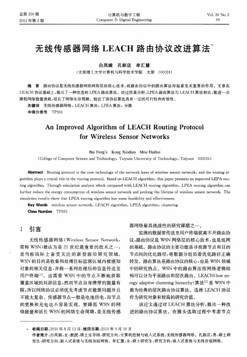
随着时间的变化,节点存活的个数图。采用LEACH 算法,节点从第420 s 开始死亡,570 s 后所有节点死亡。采用改进的算法,第一个死亡节点出现 的时间推迟到了第 550s,到595 s 所有节点死亡全部死亡,改进的算法将第一 个节点死亡的时间向后推迟,因此延长了网络生存时间。这是因为簇头的 均匀分布可以避免各节点与簇头之间距离差异而引起的耗能的差距,并且 选取簇头时,依据节点的剩余能量水平,这样可以避免能量少的节点当选 为簇头。
E 34 26 22 16
显然,采用LEACH算法时,整个网络的生命周期将小于4轮。从 上面的分析不难看出,LEACH算法进行第四轮簇头选取时,没有 考虑到节点的剩余能量及其工作能耗,导致剩余能量小于工作能 耗的节点D当选为簇头,使节点D的能量过早衰竭,网络的生命周 期也随之结束。若结合考虑节点的位置信息,使靠近簇结构中心 位置且剩余能量较多的节点有更多机会成为簇头,无疑将有效延 长网络的生命周期。在改进方面我们考虑到能量的问题并作出了改进。
2 .未考虑节点分布密度时存在的问题
基站
应尽可能使密集分布区域中的节点比稀疏分布区域中的 节点具有更大当选为簇头的概率,使得密集分布区域比 稀疏分布区域产生更多簇头,并且每个簇中成员节点数 目大致相同,从而保证各簇头的工作能耗也相对均衡。
BACK
LEACH算法的改进
考虑了节点的剩余能量,为了避免节点在剩余能量 很小时也会被选为簇头节点。 1.簇头之间最优距离D 的计算 首先假设探测区域 A 是边长为L 的正方形区域,理想状态下k 个簇首节点应当完全覆盖区域A,则应该kπ(D/2)2 = C*L2。 其中C>=1 是一个常数,是为了充分保证群首节点能覆盖区域 A而设置的。由此得出平均意义下每个群首覆盖的区域半径应 该为
无线传感器网络改进的LEACH-ID算法

无线传感器网络改进的LEACH-ID算法摘要:分析了经典的分簇路由协议LEACH,针对LEACH中的簇头个数、簇中成员数太多或太少,从而导致节点加快死亡、网络能量利用率低的问题,通过计算最优簇头数、控制簇中成员数,均衡了网络中能量的消耗,提高了网络能量的利用率,延长了网络寿命。
同时给出一种简单的产生临时ID的方法,保证了相互间较大概率的互异性。
仿真实验结果表明,LEACH??ID协议与LEACH 协议相比延长了网络寿命,推迟了第一个死亡节点出现的时间,提高了能量利用率。
?ス丶?词:无线传感器网络;LEACH协议;簇头;临时ID号?ブ型挤掷嗪牛? TP393.04; TN915.04文献标志码:A英文标题??Improved LEACH??ID algorithm for wireless sensor networks?び⑽淖髡呙?SHI Ye??ling, CHEN Bin??bing?び⑽牡刂?(School of Electrical Engineering and Information, Sichuan University, Chengdu Sichuan 610065, China英文摘要)??Abstract:Classical clustering communication protocol of LEACH was analyzed. Concerning the problem that the amounts of cluster heads andtoo many or too few members of the cluster may cause the accelerated death of the nodes and low energy use of the network, by calculating optimal clustering heads and controlling members of the cluster, the consumed energy was balanced, the usage rate of the network energy was improved and the network??s lifetime was prolonged. At the same time, a simple and effective method of assigning temporary ID was given, which can assure the dissimilarity of the IDs with large probability. The simulation results indicate that, compared with LEACH, LEACH??ID extends the lifetime of network, delays the first node??s death time, and enhances the energy efficiency.英文关键词??Key words:Wireless Sensor Network (WSN); LEACH protocol; clusterhead; temporary ID number??0 引言??由于工作环境和自身构造所限,无线传感器网络(Wireless Sensor Network, WSN)传感器节点的计算、通信能力及能量都十分有限,对于节点的更换和充电也较难实现。
述leach算法的工作流程

述leach算法的工作流程下载温馨提示:该文档是我店铺精心编制而成,希望大家下载以后,能够帮助大家解决实际的问题。
文档下载后可定制随意修改,请根据实际需要进行相应的调整和使用,谢谢!并且,本店铺为大家提供各种各样类型的实用资料,如教育随笔、日记赏析、句子摘抄、古诗大全、经典美文、话题作文、工作总结、词语解析、文案摘录、其他资料等等,如想了解不同资料格式和写法,敬请关注!Download tips: This document is carefully compiled by theeditor. I hope that after you download them,they can help yousolve practical problems. The document can be customized andmodified after downloading,please adjust and use it according toactual needs, thank you!In addition, our shop provides you with various types ofpractical materials,such as educational essays, diaryappreciation,sentence excerpts,ancient poems,classic articles,topic composition,work summary,word parsing,copy excerpts,other materials and so on,want to know different data formats andwriting methods,please pay attention!LEACH 算法是一种基于聚类的路由协议,它的工作流程如下:1. 初始化阶段。
简述LEACH算法的基本原理。

简述LEACH算法的基本原理。
LEACH(Low Energy Adaptive Clustering Hierarchy)算法是一种无线传感器网络中常用的能量有效的数据聚集协议。
其基本原理是将传感器节点分为若干个簇,每个簇有一个簇头节点,簇头节点负责收集和汇总本簇内的数据并将其传输到基站,从而减少无线传输的能量消耗,延长网络寿命。
LEACH算法的具体实现步骤如下:
1. 初始阶段:每个节点随机选择一个数值作为阈值,若节点的能量水平高于该阈值,则该节点有可能成为簇头节点。
2. 簇头节点选择阶段:每个节点通过计算与其距离的平方和来确定与其最近的簇头节点,并将自己加入该簇头节点所在的簇中。
每个簇头节点根据自己的能量水平计算出一个概率值,该概率值与其他节点的能量水平成反比,能量水平越高的节点成为簇头节点的概率越小。
簇头节点将自己的概率值广播给其他节点,每个节点通过比较自己的概率值和簇头节点的概率值来决定是否成为簇头节点。
3. 簇内通信阶段:每个节点将数据发送给其所在的簇头节点,簇头节点负责汇总和压缩数据,并将数据传输到基站。
4. 轮换阶段:为了平衡能量消耗,每个簇头节点轮流充当簇头节点,其他节点
重新选择簇头节点。
LEACH算法的优点是能够有效地减少能量消耗,延长网络寿命,同时具有良好的可扩展性和自适应性。
但是由于其随机性较强,可能导致网络中出现簇头节点密集或稀疏的情况,从而影响网络性能。
WSN中LEACH协议源码分析报告

WSN中LEACH协议源码分析分析(一)首先对wireless.tcl进行分析,先对默认的脚本选项进行初始化:set opt(chan)Channel/\VirelessChannelset opt(prop) Propagatioii/TwoRayGroundset opt(netif)PhyAVirelessPhyset opt(mac) Mac/802_l 1set opt(ifq) Qucuc/DropTail/PriQueueset opt(ll) LLset opt(ant) Antenna/OmniAntennaset opt(x) 0 。
# X dimension of the topographyset opt(y) 0。
# Y dimension of the topographyset opt(cp),H,set opt(sc) N../mobility/scene/scen-670x670-50-600-20-2u。
# scenario file set opt(ifqlen)50o # max packet in ifset opt(nn) 51。
# number of nodesset opt(secd) 0.0set opt(stop) 10.0 o # simulation timeset opt(tr) out.tr。
# trace fileset opt(rp) dsdv 。
# routing protocol scriptset opt(lm) M on H。
# log movement在这个wireless.tcl中设置了一些全局变呈::##Initialize Global Variables#set ns_ [new Simulator]set chan [new $opt(chan)]set prop [new $opt(prop)]set topo [newTopography]set tracefd [open Sopt(tr) w]Stopo Ioad_flatgrid $opt(x) $opt(y)Sprop topography Stopo这些初始化将在后而的使用中用到,该文件最重要的是创建leach 17点:创建方法如下:} elseif { [string compare Sopt(rp) M leach,,]==0} {for {set i 0} {$i < $opt(nn) } {incr i} {leach-create-mobile-node $i}如果路由协议是leach协议,则在Uamps.tcl中调用leach-create-mobile-node方法创建leach节点。
birch算法代码

birch算法代码Birch算法是一种用于聚类的算法,它是一种基于模型的方法,可以有效地处理大规模的数据集。
该算法由David Arthur和William Vitter于1996年提出,是一种适用于大规模数据的分布式聚类算法。
以下是一个使用Python实现的Birch算法的示例代码:```pythonimport numpy as npimport randomimport copyclass BirchClustering:def __init__(self, k, n_clusters, n_neighbors):self.k = k # 聚类个数self.n_clusters = n_clusters # 聚类数量self.n_neighbors = n_neighbors # 邻居数量self.clusters = [] # 存储聚类结果的列表self.trees = [] # 存储每个聚类树的列表def generate_initial_clusters(self, data):# 使用k-means算法生成初始聚类中心initial_clusters = np.random.choice(len(data), self.k, replace=False)clusters = self.kmeans(data, initial_clusters)return clustersdef split_tree(self, tree):# 分割树并返回新的树和剩余的数据点new_clusters = []remaining_data = []for child in tree.children:new_clusters += self.split_tree(child)remaining_data += tree.datareturn new_clusters, remaining_datadef fit_tree(self, clusters):# 根据聚类结果生成树,并返回树对象root = TreeNode(len(clusters), clusters)for i in range(self.k):for cluster in clusters:if cluster[i] == 1:breakcluster = copy.deepcopy(clusters[i])new_cluster = self.split_cluster(cluster)root.children.append(TreeNode(new_cluster))return rootdef split_cluster(self, cluster):# 分割集群并返回分割后的集群和剩余的数据点new_cluster = []remaining_data = []for point in cluster:if point not in remaining_data:new_cluster += [point]else:remaining_data += [point]return new_cluster, remaining_data[:],remaining_data[len(new_cluster)] # 数据点和剩余点重合并赋值给一个新列表返回。
LEACH分簇算法实现和能量控制算法实现

一:题目1、在给定WSN的节点数目(100)前提下,节点随机分布,按照LEACH算法,实现每一轮对WSN的分簇。
记录前K轮(k=10)时,网络的分簇情况,即每个节点的角色(簇头或簇成员)。
标记节点之间的关系,标记其所属的簇头。
2、在1的基础上,增加能量有效性控制:给定的所有节点具有相同的能量,考察第一个节点能量耗尽出现在第几轮。
节点的能量消耗仅考虑关键的几次通信过程,其他能量消耗不计。
通信过程能量消耗规则如下:Setup:簇成元:每次收到候选簇头信息-1,每个候选簇头仅被收集一次;通知簇头成为其成员,发送信息-2。
候选簇头:被簇成元接收信息,即发送信息,能量-2;被通知成为簇头,接收信息能量-1。
Steady:每个簇成员每轮向簇头发送10次数据,每次成员能量-2,簇头能量-1。
二:目的(1)在固定节点个数的前提下,仿真LEACH算法的分簇过程。
(2)在上述节点个数和分簇算法的前提下,计算节点的能量消耗,判断能量消耗到0的节点出现在第几轮。
三:方法描述(1)LEACH分簇簇头选举初始阶段,每个节点根据所建议网络簇头的百分比(事先确定)和节点已经成为簇头的次数来确定自己是否当选为簇头。
每个节点产生一个0-1的随机数字,如果该数字小于阈值,节点成为当前轮的簇头。
阈值其他其中,P为预期的簇头百分比,r为当前轮数,G是最近1/p轮里没有成为簇头的节点的集合。
首先确定传感器网络中的节点个数为100个,并对所有节点初始化其三个属性,分别有type(节点类型),selected(是否当选过簇头)和temp_rand(随机数)。
设定簇头产生概率p=0.08。
算法步骤如下:Step1:随机生成100个节点位置,并赋值随机数temp_rand,设置type和selected为’N’。
Step2:将所有selected为’N’的节点随机值与做比较,若temp_rand小于等于则转向Step3,否则转向Step4。
Step3:表明节点当选为簇头节点,将type赋值’C’, selected赋值’O’。
leach协议簇头计算公式的详细计算过程

leach协议簇头计算公式的详细计算过程Leach 协议是一种用于无线传感器网络的分簇路由协议,其中簇头的选择是一个关键环节。
下面咱们就来详细聊聊 Leach 协议簇头计算公式的计算过程。
在 Leach 协议中,簇头的选择可不是随便定的。
它有一套自己的计算公式,这个公式的目的就是为了让网络中的节点能够相对公平、有效地承担起簇头的职责,从而优化整个网络的性能。
先来说说这个公式里涉及到的一些参数。
比如说,有节点成为簇头的概率 P,网络中节点的总数 N,还有已经轮数 r 等等。
具体的计算公式是这样的:T(n) = P / (1 - P * (r mod (1 / P))) ,当 n ∈ G这里面,T(n) 表示节点 n 成为簇头的阈值,G 是在这一轮还没有被选为簇头的节点集合。
那这个公式到底咋用呢?咱来举个例子哈。
比如说一个无线传感器网络里,一共有 100 个节点,设定节点成为簇头的概率 P 是 0.1,现在已经进行到第 5 轮了。
那咱们来算一算节点 20 这一轮成为簇头的可能性。
首先算 (r mod (1 / P)) ,也就是 5 mod (1 / 0.1) = 5 mod 10 = 5 。
然后算 1 - P * (r mod (1 / P)) ,也就是 1 - 0.1 * 5 = 0.5 。
最后算 T(20) ,也就是 0.1 / 0.5 = 0.2 。
如果随机生成的一个 0 到 1 之间的数小于 0.2,那节点 20 就在这一轮被选为簇头啦。
在实际的应用中,这个公式可不是光算算就行的。
比如说,网络中的节点分布不均匀,有的地方节点密集,有的地方稀疏。
在节点密集的区域,如果按照这个公式简单计算,可能会导致簇头过于集中,这样就会加重某些区域的通信负担,影响整个网络的性能。
我之前就碰到过这样一个情况。
在一个监测森林环境的无线传感器网络中,由于树木分布的影响,有些区域的节点比较集中。
按照最初的 Leach 协议簇头计算公式选择簇头,结果就发现那些节点密集的区域能耗特别快,数据传输也不太稳定。
LEACH算法仿真结果

仿真一:在100*100 的区域内随机生成100 个节点 ( matlab 仿真代码:clear;xm=100;%x 轴范围ym=100;%y 轴范围sink.x=0.5*xm;% 基站x 轴50sink.y=0.5*ym;% 基站y 轴50n=100;E0=0.02;for i=1:1:nS(i).xd=rand(1,1)*xm;S(i).yd=rand(1,1)*ym;S(i).G=0;% 每一周期结束此变量为0 S(i).E=E0;% 设置初始能量为E0 S(i).type='N';% 节点类型为普通plot(S(i).xd,S(i).yd,'o');hold on;end%设置SINK 节点的坐标S(n+1).xd=sink.x;S(n+1).yd=sink.y;plot(S(n+1).xd,S(n+1).yd,'*');% 绘制基站节点仿真结果图片:‘ O'代表随机散布的节点,’* '代表SINK节点)100. CJ ■-1H I L IL L L L* Q-O90 L r-.门 c ° 0』亠1E 小■-80 —0 QC O Q70 1”o o o QC0°C Q60 O J」u「一A o50 -• *oO o □oo o40 —0 oo O30O ccP c 」。
° % 020 = c C |2 7 Co o c W10Q_ v? O0 Q n0 i J. Qn L f r i f r r0 10 20 30 40 50 60 70 80 90 100仿真二:LEACH分簇效果图(matlab代码见附件)仿真结果:(p=0.1)1、簇头个数14.100905I ctJ_ oE £L*1 L1(g80 K J*QQ o70 一o-60 -辛-50 -如宀七—**0 Q r-h.40 一土7 o一30 ”•=t=-■o o <b l' l20 --*10 k-/-1r J i r r 1 t〕1! 一r0 10 20 30 40 50 60 70 80 90 100100 2、簇头个数:113、簇头个数:12100厂 1I [1L.1 IIr c奋L90 -卡Q- 80■*却o■70 「4oQQO 160 po+ oQ0 OQO50■40 -Q0 Q QJ|O Q-Q+- 30 --ooi 內 co ◎o20l' wQ10 一_ j-c0 ■ ( L i(JLj rr t L10 2030405060 70 80 90 1004、簇头个数:10100£ L ■ L O*OoI Q IcO- **oJ 0"皓 + jgo o l;.°5Q Q*4=-c O「■■--* r ?,-Xf )r~j%QOJi『1LJTr Lf L1009080 70 60 5040 30 20 1010 20 30 405060708090(p=0.05) 1、簇头=6100 90 80 70 60 50 40 30 20 102、簇头=7L.1七L B 1 1*lL L--o o*fjftzjC0Q*—*)°如-■-*一* o cP!. iex-tr r I rr r rr 90 80 70 6050 4030 20 1010 20 30 40 5060 70809010010 20 30 40 50 60 70 80 90 10010006 08 0Z 09 09 017OSOSOL4-OLOSOS0170909OZ0806 00 L 06 08 OZ 09 09 017 OS 0 乙OL 010203040506070 8090100xLEACH分簇算法成簇效果图 100 — __ Q2 Q90一fj__fj-簇头~^宰80 — 普通节点一尸 O 话70 —G + 苇广Q X )QOQOocW-o 60Q辛 0-oy50 —SINK 节点—>七> *40 PoO30C51f °。
无线传感器网络LEACH路由协议改进算法
计算机 与数 字工 程
C mp tr& Dii lEn ie r g o ue gt gn ei a n
Vo_ 9No 2 l3 .
44
2 1 年第 2 01 期
无线 传 感器 网络 L A H 路 由协 议 改 进 算 法 E C
白凤娥 孔新店 牟汇 慧
K y W o d wiee ssn o ewo k e rs rls e s rn t r ,LE ACH lo i m ,LP ag rt h EA lo i m ,cu trn ag rt h lse ig
Cl s m b r TP3 3 a s Nu e 9
1 引 言
太原 002) 3 0 4 ( 原理工大学计算机与科学技术学院 太
摘
要
路 由协议是无线传感器 网络 网络层 的核心技 术 , 而路 由协议 中的路 由算 法却起 着至关重 要的作用 。文章 在
L AC 协议 基础 上 , E H 提出了一种 改进 的 L E P A路 由算法 。经过仿 真分析 , P A路 由算法与 L AC 算法相 比, LE E H 能进一 步 降低网络能量消耗 , 延长了 网络生存周期 。验证 了该 协议 算法具有一定的可行性和有效性 。
无线 传 感 器 网 络 ( rl sS n o t r , Wi e e srNewo k es 简称 WS 被认 为是 2 世 纪最 重 要 的技 术 之 一 , N) 1 是 当前 国 际 上 备 受 关 注 的 新 型 前 沿 研 究 领 域 。 WS 的 目的是 收集 和处 理 目标 监测 区域 内被感 知 N
关键词 无 线传感器 网络 ; E C 算法 ; P A算法 ; L A H LE 分簇
leach协议matlab仿真代码

leach协议matlab仿真代码LEACH協議clear;%清除內存變量xm=100;%x軸範圍ym=100;%y軸範圍sink.x=0.5*xm;%基站x軸sink.y=0.5*ym;%基站y軸n=100;%節點總數p=0.1;%簇頭概率E0=0.02;%初始能量ETX=50*0.000000000001;%傳輸能量,每bitERX=50*0.000000000001;%接收能量,每bitEfs=10*0.000000000001;%耗散能量,每bitEDA=5*0.000000000001;%融合能耗,每bitcc=0.6;%融合率rmax=1000;%總輪數CM=32;%控制信息⼤⼩DM=4000;%數據信息⼤⼩figure(1);%顯⽰圖⽚for i=1:1:nS(i).xd=rand(1,1)*xm;S(i).yd=rand(1,1)*ym;S(i).G=0;%每⼀週期結束此變量為0S(i).E=E0;%設置初始能量為E0S(i).type='N';%節點類型為普通plot(S(i).xd,S(i).yd,'o');hold on;%保持所畫的圖像end%為每個節點隨機分配坐標,並設置初始能量為E0,節點類型為普通S(n+1).xd=sink.x;S(n+1).yd=sink.y;plot(S(n+1).xd,S(n+1).yd,'x');%繪製基站節點flag_first_dead=0;%第⼀個死亡節點的標誌變量for r=1:1:rmax%開始每輪循環r+1%顯⽰輪數if(mod(r,round(1/p))==0)for i=1:1:nS(i).G=0;endend%如何輪數正好是⼀個週期的整數倍,則設置S(i).E為0hold off;%每輪圖⽚重新繪製cluster=0;%初始簇頭數為0dead=0;%初始死亡節點數為0figure(1);for i=1:1:nif(S(i).E<=0)plot(S(i).xd,S(i).yd,'red .');dead=dead+1;%將能量⼩於等於0的節點繪製成紅⾊,並將死亡節點數增加1if(dead==1)if(flag_first_dead==0)first_dead=r %第⼀個節點的死亡輪數save ltest, first_dead;flag_first_dead=1;endend%將能量⼩於等於0的節點繪製成紅⾊,並將死亡節點數增加1hold on;elseS(i).type='N';plot(S(i).xd,S(i).yd,'o');%繪製其他節點hold on;endendplot(S(n+1).xd,S(n+1).yd,'x');%繪製基站Dead(r+1)=dead; %每輪有死亡節點數save ltest, Dead(r+1);%將此數據存⼊ltest⽂件for i=1:1:nif(S(i).E>0)if(S(i).G<=0)temp_rand=rand;%取⼀個隨機數if(temp_rand<=(p/(1-p*mod(r,round(1/p)))))%如果隨機數⼩於等於S(i).type='C';%此節點為此輪簇頭S(i).G=round(1/p)-1;%S(i).G設置為⼤於0,此週期不能再被選擇為簇頭cluster=cluster+1;%簇頭數加1C(cluster).xd=S(i).xd;C(cluster).yd=S(i).yd;%將此節點標誌為簇頭plot(S(i).xd,S(i).yd,'k*');%繪製此簇頭distance=sqrt((S(i).xd-(S(n+1).xd))^2+(S(i).yd-(S(n+1).yd))^2);%簇頭到基站的距離C(cluster).distance=distance;%標誌為此簇頭的距離C(cluster).id=i; %此簇頭的節點idpacket_To_BS(cluster)=1;%發送到基站的數據包數為1endendendendCH_Num(r+1)=cluster; %每輪的簇頭數save ltest,CH_Num(r+1);%保存每輪簇頭數到ltestfor i=1:1:nif(S(i).type=='N'&&S(i).E>0)%對每個能量⼤於0且⾮簇頭節點min_dis=sqrt((S(i).xd-(C(1).xd))^2+(S(i).yd-(C(1).yd))^2);%計算此節點到簇頭1的距離min_dis_cluster=1;for c=2:1:clustertemp=sqrt((S(i).xd-(C(c).xd))^2+(S(i).yd-(C(c).yd))^2);if(temp<min_dis)min_dis=temp;min_dis_cluster=c;endend%選擇此幾點到哪個簇頭的距離最⼩packet_To_BS(min_dis_cluster)=packet_To_BS(min_dis_cluster)+1;%將此節點加⼊的簇 %頭節點數據包數加1Er1=ERX*CM*(cluster+1);%此節點接收各個簇頭的控制信息%此節點加⼊的簇的簇頭時隙控制信息的總接收能耗Et1=ETX*(CM+DM)+Efs*(CM+DM)*min_dis*min_dis;%此節點發送加⼊信息和發送數據信息 %到簇頭的能耗S(i).E=S(i).E-Er1-Et1;%此輪後的剩餘能量endendfor c=1:1:cluster%各個簇頭packet_To_BS(c);%簇頭需發送到基站的數據包個數CEr1=ERX*CM*(packet_To_BS(c)-1);%收到此簇各個節點加⼊信息的能耗CEr2=ERX*DM*(packet_To_BS(c)-1);%收到此簇各個節點數據信息的能耗CEt1=ETX*CM+Efs*CM*(sqrt(xm*ym))*(sqrt(xm*ym));%此簇頭廣播成簇信息的能耗CEt2=(ETX+EDA)*DM*cc*packet_To_BS(c)+Efs*DM*cc*packet_To_BS(c)*C(c).distance*C(c).distance;%簇頭將所以數據融合後發往基站的能耗S(C(c).id).E=S(C(c).id).E-CEr1-CEr2-CEt1-CEt2;%此輪後簇頭的剩餘能量endfor i=1:1:nR(r+1,i)=S(i).E; %每輪每節點的剩餘能量% save ltest,R(r+1,i);%保存此數據到ltestendhold on;end。
LEACH算法原理详解

Copyright2000IEEE.Published in the Proceedings of the Hawaii International Conference on System Sciences,January4-7,2000,Maui,Hawaii. Energy-Efficient Communication Protocol for Wireless Microsensor Networks Wendi Rabiner Heinzelman,Anantha Chandrakasan,and Hari BalakrishnanMassachusetts Institute of TechnologyCambridge,MA02139wendi,anantha,hari@AbstractWireless distributed microsensor systems will enable the reliable monitoring of a variety of environments for both civil and military applications.In this paper,we look at communication protocols,which can have significant im-pact on the overall energy dissipation of these networks. Based on ourfindings that the conventional protocols of direct transmission,minimum-transmission-energy,multi-hop routing,and static clustering may not be optimal for sensor networks,we propose LEACH(Low-Energy Adap-tive Clustering Hierarchy),a clustering-based protocol that utilizes randomized rotation of local cluster base stations (cluster-heads)to evenly distribute the energy load among the sensors in the network.LEACH uses localized coordi-nation to enable scalability and robustness for dynamic net-works,and incorporates data fusion into the routing proto-col to reduce the amount of information that must be trans-mitted to the base station.Simulations show that LEACH can achieve as much as a factor of8reduction in energy dissipation compared with conventional routing protocols. In addition,LEACH is able to distribute energy dissipation evenly throughout the sensors,doubling the useful system lifetime for the networks we simulated.1.IntroductionRecent advances in MEMS-based sensor technology, low-power analog and digital electronics,and low-power RF design have enabled the development of relatively in-expensive and low-power wireless microsensors[2,3,4]. These sensors are not as reliable or as accurate as their ex-pensive macrosensor counterparts,but their size and cost enable applications to network hundreds or thousands of these microsensors in order to achieve high quality,fault-tolerant sensing networks.Reliable environment monitor-ing is important in a variety of commercial and military applications.For example,for a security system,acoustic,seismic,and video sensors can be used to form an ad hoc network to detect intrusions.Microsensors can also be used to monitor machines for fault detection and diagnosis.Microsensor networks can contain hundreds or thou-sands of sensing nodes.It is desirable to make these nodes as cheap and energy-efficient as possible and rely on their large numbers to obtain high quality work pro-tocols must be designed to achieve fault tolerance in the presence of individual node failure while minimizing en-ergy consumption.In addition,since the limited wireless channel bandwidth must be shared among all the sensors in the network,routing protocols for these networks should be able to perform local collaboration to reduce bandwidth requirements.Eventually,the data being sensed by the nodes in the net-work must be transmitted to a control center or base station, where the end-user can access the data.There are many pos-sible models for these microsensor networks.In this work, we consider microsensor networks where:The base station isfixed and located far from the sen-sors.All nodes in the network are homogeneous and energy-constrained.Thus,communication between the sensor nodes and the base station is expensive,and there are no“high-energy”nodes through which communication can proceed.This is the framework for MIT’s-AMPS project,which focuses on innovative energy-optimized solutions at all levels of the system hierarchy,from the physical layer and communica-tion protocols up to the application layer and efficient DSP design for microsensor nodes.Sensor networks contain too much data for an end-user to process.Therefore,automated methods of combining or aggregating the data into a small set of meaningful informa-tion is required[7,8].In addition to helping avoid informa-tion overload,data aggregation,also known as data fusion, can combine several unreliable data measurements to pro-duce a more accurate signal by enhancing the common sig-nal and reducing the uncorrelated noise.The classification performed on the aggregated data might be performed by a human operator or automatically.Both the method of per-forming data aggregation and the classification algorithm are application-specific.For example,acoustic signals are often combined using a beamforming algorithm[5,17]to reduce several signals into a single signal that contains the relevant information of all the individual rge en-ergy gains can be achieved by performing the data fusion or classification algorithm locally,thereby requiring much less data to be transmitted to the base station.By analyzing the advantages and disadvantages of con-ventional routing protocols using our model of sensor net-works,we have developed LEACH(Low-Energy Adaptive Clustering Hierarchy),a clustering-based protocol that min-imizes energy dissipation in sensor networks.The key fea-tures of LEACH are:Localized coordination and control for cluster set-up and operation.Randomized rotation of the cluster“base stations”or “cluster-heads”and the corresponding clusters.Local compression to reduce global communication. The use of clusters for transmitting data to the base sta-tion leverages the advantages of small transmit distances for most nodes,requiring only a few nodes to transmit far distances to the base station.However,LEACH out-performs classical clustering algorithms by using adaptive clusters and rotating cluster-heads,allowing the energy re-quirements of the system to be distributed among all the sensors.In addition,LEACH is able to perform local com-putation in each cluster to reduce the amount of data that must be transmitted to the base station.This achieves a large reduction in the energy dissipation,as computation is much cheaper than communication.2.First Order Radio ModelCurrently,there is a great deal of research in the area of low-energy radios.Different assumptions about the radio characteristics,including energy dissipation in the transmit and receive modes,will change the advantages of different protocols.In our work,we assume a simple model where the radio dissipates nJ/bit to run the transmit-ter or receiver circuitry and pJ/bit/m for the transmit amplifier to achieve an acceptableFor example,the Bluetooth initiative[1]specifies700Kbps radios that operate at2.7V and30mA,or115nJ/bit.Operationenergy loss due to channel transmission.Thus,to trans-mit a-bit message a distance using our radio model,the radio expends:(1) and to receive this message,the radio expends:(2) For these parameter values,receiving a message is not a low cost operation;the protocols should thus try to minimize not only the transmit distances but also the number of transmit and receive operations for each message.We make the assumption that the radio channel is sym-metric such that the energy required to transmit a message from node A to node B is the same as the energy required to transmit a message from node B to node A for a given SNR.For our experiments,we also assume that all sensors are sensing the environment at afixed rate and thus always have data to send to the end-user.For future versions of our protocol,we will implement an”event-driven”simulation, where sensors only transmit data if some event occurs in the environment.3.Energy Analysis of Routing ProtocolsThere have been several network routing protocols pro-posed for wireless networks that can be examined in the context of wireless sensor networks.We examine two such protocols,namely direct communication with the base sta-tion and minimum-energy multi-hop routing using our sen-sor network and radio models.In addition,we discuss a conventional clustering approach to routing and the draw-backs of using such an approach when the nodes are all energy-constrained.Using a direct communication protocol,each sensor sends its data directly to the base station.If the base sta-tion is far away from the nodes,direct communication will require a large amount of transmit power from each node (since in Equation1is large).This will quickly drain the battery of the nodes and reduce the system lifetime.How-ever,the only receptions in this protocol occur at the base station,so if either the base station is close to the nodes,or the energy required to receive data is large,this may be an acceptable(and possibly optimal)method of communica-tion.The second conventional approach we consider is a “minimum-energy”routing protocol.There are several power-aware routing protocols discussed in the literature[6, 9,10,14,15].In these protocols,nodes route data des-tined ultimately for the base station through intermediate nodes.Thus nodes act as routers for other nodes’data in addition to sensing the environment.These protocols dif-fer in the way the routes are chosen.Some of these proto-cols[6,10,14],only consider the energy of the transmitter and neglect the energy dissipation of the receivers in de-termining the routes.In this case,the intermediate nodes are chosen such that the transmit amplifier energy(e.g.,)is minimized;thus nodeA would transmit to node C through nodeB if and only if:(3) or(4) However,for this minimum-transmission-energy(MTE) routing protocol,rather than just one(high-energy)trans-mit of the data,each data message must go through(low-energy)transmits and receives.Depending on the rela-tive costs of the transmit amplifier and the radio electronics, the total energy expended in the system might actually be greater using MTE routing than direct transmission to the base station.To illustrate this point,consider the linear network shown in Figure2,where the distance between the nodes is.If we consider the energy expended transmitting a sin-gle-bit message from a node located a distance froma(6) Therefore,direct communication requires less energy than MTE routing if:(7)Using Equations1-6and the random100-node network shown in Figure3,we simulated transmission of data from every node to the base station(located100m from the clos-est sensor node,at(x=0,y=-100))using MATLAB.Figure4 shows the total energy expended in the system as the net-work diameter increases from10m10m to100m100 m and the energy expended in the radio electronics(i.e., )increases from10nJ/bit to100nJ/bit,for the sce-nario where each node has a2000-bit data packet to send to the base station.This shows that,as predicted by our anal-ysis above,when transmission energy is on the same order as receive energy,which occurs when transmission distance is short and/or the radio electronics energy is high,direct transmission is more energy-efficient on a global scale than MTE routing.Thus the most energy-efficient protocol to use depends on the network topology and radio parameters of the system.−25−20−15−10−5051015202505101520253035404550Figure 3.100-node random network.Figure 4.Total energy dissipated in the 100-node random network using direct commu-nication and MTE routing (i.e.,and ).pJ/bit/m ,and the mes-sages are 2000bits.Figure 5.System lifetime using direct trans-mission and MTE routing with 0.5J/node.It is clear that in MTE routing,the nodes closest to the base station will be used to route a large number of data messages to the base station.Thus these nodes will die out quickly,causing the energy required to get the remaining data to the base station to increase and more nodes to die.This will create a cascading effect that will shorten system lifetime.In addition,as nodes close to the base station die,that area of the environment is no longer being monitored.To prove this point,we ran simulations using the random 100-node network shown in Figure 3and had each sensor send a 2000-bit data packet to the base station during each time step or “round”of the simulation.After the energy dissipated in a given node reached a set threshold,that node was considered dead for the remainder of the simulation.Figure 5shows the number of sensors that remain alive after each round for direct transmission and MTE routing with each node initially given 0.5J of energy.This plot shows that nodes die out quicker using MTE routing than direct transmission.Figure 6shows that nodes closest to the base station are the ones to die out first for MTE routing,whereas nodes furthest from the base station are the ones to die out first for direct transmission.This is as expected,since the nodes close to the base station are the ones most used as “routers”for other sensors’data in MTE routing,and the nodes furthest from the base station have the largest transmit energy in direct communication.A final conventional protocol for wireless networks is clustering,where nodes are organized into clusters that communicate with a local base station,and these local base stations transmit the data to the global base station,where it is accessed by the end-user.This greatly reduces the dis-tance nodes need to transmit their data,as typically the local base station is close to all the nodes in the cluster.−25−20−15−10−5051015202505101520253035404550X−coordinateY −c o o r d i n a t eFigure 6.Sensors that remain alive (circles)and those that are dead (dots)after 180rounds with 0.5J/node for (a)direct trans-mission and (b)MTE routing.Thus,clustering appears to be an energy-efficient commu-nication protocol.However,the local base station is as-sumed to be a high-energy node;if the base station is an energy-constrained node,it would die quickly,as it is be-ing heavily utilized.Thus,conventional clustering would perform poorly for our model of microsensor networks.The Near Term Digital Radio (NTDR)project [12,16],an army-sponsored program,employs an adaptive clustering approach,similar to our work discussed here.In this work,cluster-heads change as nodes move in order to keep the network fully connected.However,the NTDR protocol is designed for long-range communication,on the order of 10s of kilometers,and consumes large amounts of power,on the order of 10s of Watts.Therefore,this protocol also does not fit our model of sensor networks.4.LEACH:Low-Energy Adaptive Clustering HierarchyLEACH is a self-organizing,adaptive clustering protocol that uses randomization to distribute the energy load evenly among the sensors in the network.In LEACH,the nodes organize themselves into local clusters,with one node act-ing as the local base station or cluster-head .If the cluster-heads were chosen a priori and fixed throughout the system lifetime,as in conventional clustering algorithms,it is easy to see that the unlucky sensors chosen to be cluster-heads would die quickly,ending the useful lifetime of all nodes belonging to those clusters.Thus LEACH includes random-ized rotation of the high-energy cluster-head position such that it rotates among the various sensors in order to not drain the battery of a single sensor.In addition,LEACH performs local data fusion to “compress”the amount of data being sent from the clusters to the base station,further reducing energy dissipation and enhancing system lifetime.Sensors elect themselves to be local cluster-heads at any given time with a certain probability.These cluster-head nodes broadcast their status to the other sensors in the network.Each sensor node determines to which clus-ter it wants to belong by choosing the cluster-head that re-quires the minimum communication energy .Once all the nodes are organized into clusters,each cluster-head creates a schedule for the nodes in its cluster.This allows the radio components of each non-cluster-head node to be turned off at all times except during its transmit time,thus minimizing the energy dissipated in the individual sensors.Once the cluster-head has all the data from the nodes in its cluster,the cluster-head node aggregates the data and then transmits the compressed data to the base station.Since the base station is far away in the scenario we are examining,this is a high energy transmission.However,since there are only a few cluster-heads,this only affects a small number of nodes.As discussed previously,being a cluster-head drains the battery of that node.In order to spread this energy usage over multiple nodes,the cluster-head nodes are not fixed;rather,this position is self-elected at different time intervals.Thus a set of nodes might elect themselves cluster-heads at time ,but at time a new set of nodes elect themselves as cluster-heads,as shown in Figure 7.The de-cision to become a cluster-head depends on the amount of energy left at the node.In this way,nodes with more en-ergy remaining will perform the energy-intensive functions of the network.Each node makes its decision about whether to be a cluster-head independently of the other nodes in the05101520253035404550Figure 7.Dynamic clusters:(a)cluster-head nodes =at time (b)cluster-head nodes=at time .All nodes marked with a given symbol belong to the same cluster,and the cluster-head nodes are marked with a .network and thus no extra negotiation is required to deter-mine the cluster-heads.The system can determine,a priori,the optimal number of clusters to have in the system.This will depend on sev-eral parameters,such as the network topology and the rela-tive costs of computation versus communication.We sim-ulated the LEACH protocol for the random network shown in Figure 3using the radio parameters in Table 1and a com-putation cost of 5nJ/bit/message to fuse 2000-bit messages while varying the percentage of total nodes that are cluster-heads.Figure 8shows how the energy dissipation in the system varies as the percent of nodes that are cluster-heads is changed.Note that 0cluster-heads and 100%cluster-heads is the same as direct communication.From this plot,we find that there exists an optimal percent of nodes that should be cluster-heads.If there are fewer than cluster-heads,some nodes in the network have to transmit their data very far to reach the cluster-head,causing the global energyFigure 8.Normalized total system energy dis-sipated versus the percent of nodes that are cluster-heads.Note that direct transmission is equivalent to 0nodes being cluster-heads or all the nodes being cluster-heads.in the system to be large.If there are more than cluster-heads,the distance nodes have to transmit to reach the near-est cluster-head does not reduce substantially,yet there are more cluster-heads that have to transmit data the long-haul distances to the base station,and there is less compression being performed locally.For our system parameters and topology,%.Figure 8also shows that LEACH can achieve over a fac-tor of 7reduction in energy dissipation compared to direct communication with the base station,when using the opti-mal number of cluster-heads.The main energy savings of the LEACH protocol is due to combining lossy compression with the data routing.There is clearly a trade-off between the quality of the output and the amount of compression achieved.In this case,some data from the individual sig-nals is lost,but this results in a substantial reduction of the overall energy dissipation of the system.We simulated LEACH (with 5%of the nodes being cluster-heads)using MATLAB with the random network shown in Figure 3.Figure 9shows how these algorithmscompare usingnJ/bit as the diameter of the net-work is increased.This plot shows that LEACH achieves between 7x and 8x reduction in energy compared with di-rect communication and between 4x and 8x reduction in energy compared with MTE routing.Figure 10shows the amount of energy dissipated using LEACH versus using di-rect communication and LEACH versus MTE routing as the network diameter is increased and the electronics energy varies.This figure shows the large energy savings achieved using LEACH for most of the parameter space.Network diameter (m)T o t a l e n e r g y d i s s i p a t e d i n s y s t e m (J o u l e s )Figure 9.Total system energy dissipated us-ing direct communication,MTE routing and LEACH for the 100-node random network shown in Figure 3.nJ/bit,pJ/bit/m ,and the messages are 2000bits.In addition to reducing energy dissipation,LEACH suc-cessfully distributes energy-usage among the nodes in thenetwork such that the nodes die randomly and at essentially the same rate.Figure 11shows a comparison of system lifetime using LEACH versus direct communication,MTE routing,and a conventional static clustering protocol,where the cluster-heads and associated clusters are chosen initially and remain fixed and data fusion is performed at the cluster-heads,for the network shown in Figure 3.For this exper-iment,each node was initially given 0.5J of energy.Fig-ure 11shows that LEACH more than doubles the useful sys-tem lifetime compared with the alternative approaches.We ran similar experiments with different energy thresholds and found that no matter how much energy each node is given,it takes approximately 8times longer for the first node to die and approximately 3times longer for the last node to die in LEACH as it does in any of the other protocols.The data from these experiments is shown in Table 2.The ad-vantage of using dynamic clustering (LEACH)versus static clustering can be clearly seen in Figure ing a static clustering algorithm,as soon as the cluster-head node dies,all nodes from that cluster effectively die since there is no way to get their data to the base station.While these simu-lations do not account for the setup time to configure the dynamic clusters (nor do they account for any necessary routing start-up costs or updates as nodes die),they give a good first order approximation of the lifetime extension we can achieve using LEACH.Another important advantage of LEACH,illustrated in Figure 12,is the fact that nodes die in essentially a “ran-Figure 10.Total system energy dissipated using (a)direct communication and LEACH and (b)MTE routing and LEACH for the ran-dom network shown in Figure 3.pJ/bit/m ,and the messages are 2000bits.Figure 11.System lifetime using direct trans-mission,MTE routing,static clustering,and LEACH with 0.5J/node.Table2.Lifetimes using different amounts ofinitial energy for the sensors.Energy Protocol Round last(J/node)node diesDirect1175Static Clustering673941090.5MTE42980LEACH1312Direct46815Static Clustering2401848-ing this threshold,each node will be a cluster-head at somepoint withinrounds.Thus the probability that the remainingnodes are cluster-heads must be increased,since there arefewer nodes that are eligible to become cluster-heads.Af-terrounds,all nodes are onceagain eligible to become cluster-heads.Future versions ofthis work will include an energy-based threshold to accountfor non-uniform energy nodes.In this case,we are assum-ing that all nodes begin with the same amount of energyand being a cluster-head removes approximately the sameamount of energy for each node.Each node that has elected itself a cluster-head for thecurrent round broadcasts an advertisement message to therest of the nodes.For this“cluster-head-advertisement”phase,the cluster-heads use a CSMA MAC protocol,and allcluster-heads transmit their advertisement using the sametransmit energy.The non-cluster-head nodes must keeptheir receivers on during this phase of set-up to hear the ad-vertisements of all the cluster-head nodes.After this phaseis complete,each non-cluster-head node decides the clusterto which it will belong for this round.This decision is basedon the received signal strength of the advertisement.As-suming symmetric propagation channels,the cluster-headadvertisement heard with the largest signal strength is thecluster-head to whom the minimum amount of transmittedenergy is needed for communication.In the case of ties,a random cluster-head is chosen.5.2Cluster Set-Up PhaseAfter each node has decided to which cluster it belongs, it must inform the cluster-head node that it will be a member of the cluster.Each node transmits this information back to the cluster-head again using a CSMA MAC protocol.Dur-ing this phase,all cluster-head nodes must keep their re-ceivers on.5.3Schedule CreationThe cluster-head node receives all the messages for nodes that would like to be included in the cluster.Based on the number of nodes in the cluster,the cluster-head node creates a TDMA schedule telling each node when it can transmit.This schedule is broadcast back to the nodes in the cluster.5.4Data TransmissionOnce the clusters are created and the TDMA schedule isfixed,data transmission can begin.Assuming nodes al-ways have data to send,they send it during their allocated transmission time to the cluster head.This transmission uses a minimal amount of energy(chosen based on the received strength of the cluster-head advertisement).The radio of each non-cluster-head node can be turned off un-til the node’s allocated transmission time,thus minimizing energy dissipation in these nodes.The cluster-head node must keep its receiver on to receive all the data from the nodes in the cluster.When all the data has been received, the cluster head node performs signal processing functions to compress the data into a single signal.For example,if the data are audio or seismic signals,the cluster-head node can beamform the individual signals to generate a compos-ite signal.This composite signal is sent to the base station. Since the base station is far away,this is a high-energy trans-mission.This is the steady-state operation of LEACH networks. After a certain time,which is determined a priori,the next round begins with each node determining if it should be a cluster-head for this round and advertising this information, as described in Section5.1.5.5.Multiple ClustersThe preceding discussion describes how the individual clusters communicate among nodes in that cluster.How-ever,radio is inherently a broadcast medium.As such, transmission in one cluster will affect(and hence degrade)toure13A’s transmission,while intended for Node B,corrupts any transmission to Node C.To reduce this type of interference, each cluster communicates using different CDMA codes. Thus,when a node decides to become a cluster-head,it chooses randomly from a list of spreading codes.It informs all the nodes in the cluster to transmit using this spreading code.The cluster-head thenfilters all received energy using the given spreading code.Thus neighboring clusters’radio signals will befiltered out and not corrupt the transmission of nodes in the cluster.Efficient channel assignment is a difficult problem,even when there is a central control center that can perform the necessary ing CDMA codes,while not nec-essarily the most bandwidth efficient solution,does solves the problem of multiple-access in a distributed manner.5.6.Hierarchical ClusteringThe version of LEACH described in this paper can be extended to form hierarchical clusters.In this scenario,the cluster-head nodes would communicate with“super-cluster-head”nodes and so on until the top layer of the hierarchy, at which point the data would be sent to the base station. For larger networks,this hierarchy could save a tremendous amount of energy.In future studies,we will explore the de-tails of implementing this protocol without using any sup-port from the base station,and determine,via simulation, exactly how much energy can be saved.6.ConclusionsIn this paper,we described LEACH,a clustering-based routing protocol that minimizes global energy usage by dis-tributing the load to all the nodes at different points in time. LEACH outperforms static clustering algorithms by requir-ing nodes to volunteer to be high-energy cluster-heads and adapting the corresponding clusters based on the nodes that choose to be cluster-heads at a given time.At different times,each node has the burden of acquiring data from the nodes in the cluster,fusing the data to obtain an aggregate signal,and transmitting this aggregate signal to the base sta-tion.LEACH is completely distributed,requiring no control information from the base station,and the nodes do not re-quire knowledge of the global network in order for LEACH to operate.Distributing the energy among the nodes in the network is effective in reducing energy dissipation from a global per-spective and enhancing system lifetime.Specifically,our simulations show that:LEACH reduces communication energy by as much as 8x compared with direct transmission and minimum-transmission-energy routing.Thefirst node death in LEACH occurs over8times later than thefirst node death in direct transmission, minimum-transmission-energy routing,and a static clustering protocol,and the last node death in LEACH occurs over3times later than the last node death in the other protocols.In order to verify our assumptions about LEACH,we are currently extending the network simulator ns[11]to simulate LEACH,direct communication,and minimum-transmission-energy routing.This will verify our assump-tions and give us a more accurate picture of the advantages and disadvantages of the different protocols.Based on our MATLAB simulations described above,we are confident that LEACH will outperform conventional communication protocols,in terms of energy dissipation,ease of configura-tion,and system lifetime/quality of the network.Providing such a low-energy,ad hoc,distributed protocol will help pave the way for future microsensor networks.AcknowledgmentsThe authors would like to thank the anonymous review-ers for the helpful comments and suggestions.W.Heinzel-man is supported by a Kodak Fellowship.This work was funded in part by DARPA.References[1]Bluetooth Project.,1999.[2]Chandrakasan,Amirtharajah,Cho,Goodman,Konduri,Ku-lik,Rabiner,and Wang.Design Considerations for Dis-tributed Microsensor Systems.In IEEE1999Custom In-tegrated Circuits Conference(CICC),pages279–286,May 1999.[3]Clare,Pottie,and Agre.Self-Organizing Distributed Sen-sor Networks.In SPIE Conference on Unattended Ground Sensor Technologies and Applications,pages229–237,Apr.1999.[4]M.Dong,K.Yung,and W.Kaiser.Low Power SignalProcessing Architectures for Network Microsensors.In Proceedings1997International Symposium on Low Power Electronics and Design,pages173–177,Aug.1997.[5] D.Dudgeon and R.Mersereau.Multidimensional DigitalSignal Processing,chapter6.Prentice-Hall,Inc.,1984. [6]M.Ettus.System Capacity,Latency,and Power Consump-tion in Multihop-routed SS-CDMA Wireless Networks.In Radio and Wireless Conference(RAWCON’98),pages55–58,Aug.1998.[7] D.Hall.Mathematical Techniques in Multisensor Data Fu-sion.Artech House,Boston,MA,1992.[8]L.Klein.Sensor and Data Fusion Concepts and Applica-tions.SPIE Optical Engr Press,WA,1993.[9]X.Lin and I.Stojmenovic.Power-Aware Routing in Ad HocWireless Networks.In SITE,University of Ottawa,TR-98-11,Dec.1998.[10]T.Meng and R.V olkan.Distributed Network Protocolsfor Wireless Communication.In Proc.IEEEE ISCAS,May 1998.[11]UCB/LBNL/VINT Network Simulator-ns(Version2)./ns/,1998.[12]R.Ruppe,S.Griswald,P.Walsh,and R.Martin.Near TermDigital Radio(NTDR)System.In Proceedings MILCOM ’97,pages1282–1287,Nov.1997.[13]K.Scott and N.Bambos.Routing and Channel Assignmentfor Low Power Transmission in PCS.In5th IEEE Int.Conf.on Universal Personal Communications,volume2,pages 498–502,Sept.1996.[14]T.Shepard.A Channel Access Scheme for Large DensePacket Radio Networks.In Proc.ACM SIGCOMM,pages 219–230,Aug.1996.[15]S.Singh,M.Woo,and C.Raghavendra.Power-Aware Rout-ing in Mobile Ad Hoc Networks.In Proceedings of the Fourth Annual ACM/IEEE International Conference on Mo-bile Computing and Networking(MobiCom’98),Oct.1998.[16]L.Williams and L.Emergy.Near Term Digital Radio-a FirstLook.In Proceedings of the1996Tactical Communications Conference,pages423–425,Apr.1996.[17]K.Yao,R.Hudson,C.Reed,D.Chen,and F.Lorenzelli.Blind Beamforming on a Randomly Distributed Sensor Ar-ray System.Proceedings of SiPS,Oct.1998.。
LEACH协议代码(MATLAB)

%%%%%%%%%%%%%%%%%%%%%%%%%%%%%%%%%%%%%%%%%%%%%%%%%%%%%%%%%%%%%%%%%%%%% %%%% %% SEP: A Stable Election Protocol for clustered % % heterogeneous wireless sensornetworks %% %% (c) GeorgiosSmaragdakis %% WING group, Computer Science Department, Boston University % % %% You can find full documentation and related information at: % %/sep %% %% To report your comment or any bug please send e-mail to: % %gsmaragd@ %% % %%%%%%%%%%%%%%%%%%%%%%%%%%%%%%%%%%%%%%%%%%%%%%%%%%%%%%%%%%%%%%%%%%%%% %%%%%%%%%%%%%%%%%%%%%%%%%%%%%%%%%%%%%%%%%%%%%%%%%%%%%%%%%%%%%%%%%%%%%%%% %%%% %% This is the LEACH [1] code we have used. % % The same code can be used for FAIR if m=1 % % %% [1] W.R.Heinzelman, A.P.Chandrakasan andH.Balakrishnan, %% "An application-specific protocol architecture forwireless %% microsensornetworks" %% IEEE Transactions on Wireless Communications,1(4):660-670,2002 %% % %%%%%%%%%%%%%%%%%%%%%%%%%%%%%%%%%%%%%%%%%%%%%%%%%%%%%%%%%%%%%%%%%%%%% %%%clear;%%%%%%%%%%%%%%%%%%%%%%%%%%%%%%%%PARAMETERS %%%%%%%%%%%%%%%%%%%%%%%%%%%%%Field Dimensions - x and y maximum (in meters)xm=100;ym=100;%x and y Coordinates of the Sinksink.x=0.5*xm;sink.y=0.5*ym;%Number of Nodes in the fieldn=100%Optimal Election Probability of a node%to become cluster headp=0.1;%Energy Model (all values in Joules)%Initial EnergyEo=0.5;%Eelec=Etx=ErxETX=50*0.000000001;ERX=50*0.000000001;%Transmit Amplifier typesEfs=10*0.000000000001;Emp=0.0013*0.000000000001;%Data Aggregation EnergyEDA=5*0.000000001;%Values for Hetereogeneity%Percentage of nodes than are advancedm=0.1;%\alphaa=1;%maximum number of roundsrmax=9999%%%%%%%%%%%%%%%%%%%%%%%%% END OF PARAMETERS %%%%%%%%%%%%%%%%%%%%%%%%%Computation of dodo=sqrt(Efs/Emp);%Creation of the random Sensor Networkfigure(1);for i=1:1:nS(i).xd=rand(1,1)*xm;XR(i)=S(i).xd;S(i).yd=rand(1,1)*ym;YR(i)=S(i).yd;S(i).G=0;%initially there are no cluster heads only nodesS(i).type='N';temp_rnd0=i;%Random Election of Normal Nodesif (temp_rnd0>=m*n+1)S(i).E=Eo;S(i).ENERGY=0;plot(S(i).xd,S(i).yd,'o');hold on;end%Random Election of Advanced Nodesif (temp_rnd0<m*n+1)S(i).E=Eo*(1+a)S(i).ENERGY=1;plot(S(i).xd,S(i).yd,'+');hold on;endendS(n+1).xd=sink.x;S(n+1).yd=sink.y;plot(S(n+1).xd,S(n+1).yd,'x');%First Iterationfigure(1);%counter for CHscountCHs=0;%counter for CHs per roundrcountCHs=0;cluster=1;countCHs;rcountCHs=rcountCHs+countCHs;flag_first_dead=0;for r=0:1:rmaxr%Operation for epochif(mod(r, round(1/p) )==0)for i=1:1:nS(i).G=0;S(i).cl=0;endendhold off;%Number of dead nodesdead=0;%Number of dead Advanced Nodesdead_a=0;%Number of dead Normal Nodesdead_n=0;%counter for bit transmitted to Bases Station and to Cluster Heads packets_TO_BS=0;packets_TO_CH=0;%counter for bit transmitted to Bases Station and to Cluster Heads %per roundPACKETS_TO_CH(r+1)=0;PACKETS_TO_BS(r+1)=0;figure(1);for i=1:1:n%checking if there is a dead nodeif (S(i).E<=0)plot(S(i).xd,S(i).yd,'red .'); dead=dead+1;if(S(i).ENERGY==1)dead_a=dead_a+1;endif(S(i).ENERGY==0)dead_n=dead_n+1;endhold on;endif S(i).E>0S(i).type='N';if (S(i).ENERGY==0)plot(S(i).xd,S(i).yd,'o');endif (S(i).ENERGY==1)plot(S(i).xd,S(i).yd,'+');endhold on;endendplot(S(n+1).xd,S(n+1).yd,'x');STATISTICS(r+1).DEAD=dead;DEAD(r+1)=dead;DEAD_N(r+1)=dead_n;DEAD_A(r+1)=dead_a;%When the first node diesif (dead==1)if(flag_first_dead==0)first_dead=rflag_first_dead=1;endendcountCHs=0;cluster=1;for i=1:1:nif(S(i).E>0)temp_rand=rand;if ( (S(i).G)<=0)%Election of Cluster Headsif(temp_rand<= (p/(1-p*mod(r,round(1/p)))))countCHs=countCHs+1;packets_TO_BS=packets_TO_BS+1;PACKETS_TO_BS(r+1)=packets_TO_BS;S(i).type='C';S(i).G=round(1/p)-1;C(cluster).xd=S(i).xd;C(cluster).yd=S(i).yd;plot(S(i).xd,S(i).yd,'k*');distance=sqrt( (S(i).xd-(S(n+1).xd) )^2 +(S(i).yd-(S(n+1).yd) )^2 );C(cluster).distance=distance;C(cluster).id=i;X(cluster)=S(i).xd;Y(cluster)=S(i).yd;cluster=cluster+1;%Calculation of Energy dissipateddistance;if (distance>do)S(i).E=S(i).E- ( (ETX+EDA)*(4000) +Emp*4000*( distance*distance*distance*distance ));endif (distance<=do)S(i).E=S(i).E- ( (ETX+EDA)*(4000) +Efs*4000*( distance * distance ));endendendendendSTATISTICS(r+1).CLUSTERHEADS=cluster-1;CLUSTERHS(r+1)=cluster-1;%Election of Associated Cluster Head for Normal Nodesfor i=1:1:nif ( S(i).type=='N' && S(i).E>0 )if(cluster-1>=1)min_dis=sqrt( (S(i).xd-S(n+1).xd)^2 + (S(i).yd-S(n+1).yd)^2 );min_dis_cluster=1;for c=1:1:cluster-1temp=min(min_dis,sqrt( (S(i).xd-C(c).xd)^2 +(S(i).yd-C(c).yd)^2 ) );if ( temp<min_dis )min_dis=temp;min_dis_cluster=c;endend%Energy dissipated by associated Cluster Headmin_dis;if (min_dis>do)S(i).E=S(i).E- ( ETX*(4000) + Emp*4000*( min_dis * min_dis * min_dis * min_dis));endif (min_dis<=do)S(i).E=S(i).E- ( ETX*(4000) + Efs*4000*( min_dis * min_dis));end%Energy dissipatedif(min_dis>0)S(C(min_dis_cluster).id).E = S(C(min_dis_cluster).id).E- ( (ERX + EDA)*4000 );PACKETS_TO_CH(r+1)=n-dead-cluster+1;endS(i).min_dis=min_dis;S(i).min_dis_cluster=min_dis_cluster;endendendhold on;countCHs;rcountCHs=rcountCHs+countCHs;%Code for Voronoi Cells%Unfortynately if there is a small%number of cells, Matlab's voronoi%procedure has some problems%[vx,vy]=voronoi(X,Y);%plot(X,Y,'r*',vx,vy,'b-');% hold on;% voronoi(X,Y);% axis([0 xm 0 ym]);end%%%%%%%%%%%%%%%%%%%%%%%%%%%%%%%%%%%STATISTICS %%%%%%%%%%%%%%%%%%%%%%%%%%%%%%%%%%%% %% DEAD : a rmax x 1 array of number of dead nodes/round% DEAD_A : a rmax x 1 array of number of dead Advanced nodes/round % DEAD_N : a rmax x 1 array of number of dead Normal nodes/round% CLUSTERHS : a rmax x 1 array of number of Cluster Heads/round% PACKETS_TO_BS : a rmax x 1 array of number packets send to Base Station/round% PACKETS_TO_CH : a rmax x 1 array of number of packets send to ClusterHeads/round% first_dead: the round where the first node died % % %%%%%%%%%%%%%%%%%%%%%%%%%%%%%%%%%%%%%%%%%%%%%%%%%%%%%%%%%%%%%%%%%%%%% %%%%%%%%%%%%%%%%%%。
leach协议簇头计算公式的详细计算过程

leach协议簇头计算公式的详细计算过程协议书参与方:公司名称:____________________________地址:__________________________________联系人姓名:___________________________电话号码:_____________________________电子邮件:_____________________________第二部分:背景与目的本协议的背景和目的在于确定一种有效的协议簇头计算公式,以支持____________________________(填写具体背景和目的)。
第三部分:定义与术语协议簇头:_____________________________计算公式:_____________________________参数:_________________________________第四部分:协议簇头计算公式步骤1:_____________________________计算公式:_____________________________具体参数如下:参数1:_____________________________参数2:_____________________________计算过程详细描述:_____________________________步骤2:_____________________________计算公式:_____________________________具体参数如下:参数1:_____________________________参数2:_____________________________计算过程详细描述:_____________________________步骤3:_____________________________计算公式:_____________________________具体参数如下:参数1:_____________________________参数2:_____________________________计算过程详细描述:_____________________________第五部分:实施与执行时间表与进程:_____________________________监督与反馈:_____________________________第六部分:风险管理在实施过程中可能涉及的风险和应对措施包括但不限于:风险1:_____________________________应对措施:_____________________________风险2:_____________________________应对措施:_____________________________第七部分:结算与支付费用分担:_____________________________结算方式与周期:_____________________________第八部分:保密条款保密责任:_____________________________信息披露限制:_____________________________第九部分:变更与修订任何关于本协议的变更或修订须经双方书面同意。
leach算法的详细信息

翻译英文原文的LEACH算法的详细信息LEACH的运作以“轮”来实现,每一轮开始是簇头的建立阶段,其次传输数据到基站的稳态阶段。
为了尽量减少开销,稳态阶段比簇建立阶段时间长。
5.1簇选举阶段簇头选举初始阶段,每个节点根据所建议网络簇头的百分比(事先确定)和节点已经成为簇头的次数来确定自己是否当选为簇头。
每个节点产生一个0-1的随机数字,如果该数字小于阈值T(N),节点成为当前轮的簇头。
阈值T(n)=⎪⎩⎪⎨⎧∈-其它,0,)]/1mod([*1Gnprpp其中,P为预期的簇头百分比(例如,p= 0.5),r为当前轮数,G是最近1/p轮里没有成为簇头的节点的集合。
使用这个阀值,每个节点会在1/p轮的某一轮成为簇头。
在0轮(r = 0),每个节点都有一个成为簇头的概率P。
当选为簇头的节点不能在未来的1/ P轮当选为簇头。
因此,只有较少的节点有资格当选为簇头节点,剩余节点成为簇头的概率必然增加。
1/p-1回合后对任意还没当选为簇头的节点T(n)=1,可见,1/ P的回合后,所有节点都再次有资格成为簇头。
以后的工作中,我们会考虑到非均匀能量节点的以能量为基础的阀值。
在这种情况下,我们假设所有节点具有相同初始数量的能量,每个簇头也消耗大约相同的能量。
非簇头节点必须保持他们的接收器在此选举阶段听到所有的簇头节点的广告。
这一阶段完成后,每个非簇头节点决定在本轮中加入哪一个簇头节点。
这一决定是基于对广告的接收信号强度。
假设是对称的传播信道,收到发送的广告信号强度最大的簇头就是要加入的簇头,与其通信需要的能量最小。
稳定之后表示簇头的随机选举完成了。
5.2簇建立阶段在每个节点已决定它属于哪个簇之后,它必须告知簇头节点,它将成为该簇的成员节点。
每个节点再次使用CSMA MAC协议发送这个信息反馈给簇头。
在这个阶段,所有的簇头节点必须保持他们的接收器打开。
5.3 时间表的创建簇头节点收到所有想加入该簇的节点的消息。
基于这个簇的节点的数量,簇头节点创建一个TDMA时间表告诉所有节点什么时候能开始传输数据。
Leach算法分析

Leach算法分析leach_mit结构图从wireless.tcl⽂件中分析leach的具体流程在wireless.tcl⽂件中⾸先初始化了很多⽆限仿真的配置。
引⽤了⼀些外部脚本——source tcl/lib/ns-mobilenode.tcl(主要是包含移动节点类Node/MobileNode的⼀些otcl类函数的定义)、source tcl/lib/ns-cmutrace.tcl(trace⽂件的tcl脚本)、 sourcetcl/mobility/$opt(rp).tcl(将⼏种不同的协议的具体应⽤的外部脚本引⽤,$opt(rp)是协议名称)。
当⼀些变量初始化过后,通过elseif { [string compare $opt(rp) "leach"] == 0} {for {set i 0} {$i < $opt(nn) } {incr i} {leach-create-mobile-node $i建⽴我们仿真的节点,最主要的函数是leach-create-mobile-node(这个函数的定义在uamps.tcl中)分析uamps.tcl中是如何定义节点的在uamps.tcl中初始化了bsnode的应⽤类型(Application/BSApp)、定义了⼆个能量传输模型(⾃由信道和多径衰落、Efriss_amp和Etwo_ray_amp)和很多参数。
⽽真正创建节点是在函数leach-create-mobile-node中。
⽽这个函数中调⽤了uamps.tcl中的sens_init,这个函数的功能是清除上⼀次模拟时留下的trace⽂件。
在创建节点时候,sens_init函数调⽤⼀次。
leach-create-mobile-node函数解释如下:1、节点定义:if {$id != $opt(nn_)} {puts -nonewline "$id "set node_($id) [new MobileNode/ResourceAwareNode] #将前opt(nn_)-1个点定义为⼀般节点} else {puts "($opt(nn_) == BS)"set node_($id) [new MobileNode/ResourceAwareNode $BS_NODE] #将第opt(nn_)个节点定义为最终的sink节点$node_($id) label "BS"$node_($id) label-color red}2、初始化能量:if {$id != $opt(nn_)} { #如果节点的能量相等,就将所有普通节点的能量初始化为$opt(init_energy)。
简述LEACH算法的基本原理。

简述LEACH算法的基本原理。
LEACH算法(LowenergyAdaptiveclusteringhierarchy)是一种分布式无线传感器网络的节能协议。
它由斯坦福大学的梅里亚尼教授提出,用于减少能耗的层次式聚类算法。
LEACH算法的基本原理是:首先,LEACH算法假设每个传感器结
点都有可用的电池能量和处理能力,而这些传感器结点位于一个无线传感器网络中,这样可以减少网络中结点之间的能耗。
其次,每个传感器结点在协议结束之前要经历多个时间步骤,不断重组结点之间的联系。
每个结点使用随机预测和平均相关性来识别能量消耗最低的聚类头结点。
在这个过程中,每个传感器结点会发送消息给其他结点,询问是否可以成为聚类头结点。
最后,每个结点和其他可用的结点一起形成一个簇。
聚类头结点收集数据并将其发送给数据处理中心。
当非头结点收集到足够的数据后,它们也会发送给数据处理中心。
当结点聚类结束时,它们将依次进入休眠状态,以节约能量。
因此,LEACH算法的基本原理就是利用随机预测和平均相关性来识别能量消耗最低的聚类头结点,然后在结点之间建立联系,收集数据并发送给数据处理中心,最后进入休眠状态以减少结点之间的能耗。
- 1 -。
基于LEACH的一种新的能量高效的分簇路由算法

d iI 。 6  ̄i n16 - 7 52 1 . .1 o:O3 9 .s .5 3 4 9 . 0 0 4 9 s 01 4
基于LA H的一种新 的能量 高效 的 EC 分簇路 由算法
吴 青
f 国矿 业 大学信息 与 电气工程 学院 ,江 苏 徐 州 2 10 ) 中 20 8 摘 要 :与一般 的 平 面 多跳 路 由算 法相 比 ,低 功 耗 自适 应  ̄ L AC (o n ryA at eCut ig E H L wE eg dpi ls r v en
据进 行 必要 的融合 处 理后 ,发送 到 s k 点 。过一 段 i 节 n 时间 后 ,网络 就会再 一 次 回到协 议 的建 立 阶段 ,开 始
本 文给 出 了一种 新 的路 由算 法 ,分 别对 L A H算 E C
法 中簇 首选 择设 计 了一 种新 的协议 L A H— N,并 在 E C E 此 基础 上对 簇 问路 由机制 进行 了改 进 ,设计 出了一 种 新 的L A H E — E C — N MH方法 它 根据 网络 中节 点 的剩 余 能量 ,动态 地选 择集 中式 或分 布式 分簇 算法 .可 以有
()=
过无 线 通信 的方式 形 成 的 多跳 的 自组 织 的 网络 系统 , 用 于感 知 、采集 和处 理 网络覆 盖 区域 的监 测信 息 ,并 其 中G 在最 后 的 l 轮 中未 成 为簇 首 节 点 的 集 是 , p 合 ,r 当前 的轮数 .P 是 为期 望 的簇 首 节点 在所 有传 感 器节 点 中的百分 比。假设 整个 网络 中节 点 的数量 为Ⅳ,
【 (- )/ K 1 12 3 D D 一K 1 ]2 - )(= , , … ) 2(
- 1、下载文档前请自行甄别文档内容的完整性,平台不提供额外的编辑、内容补充、找答案等附加服务。
- 2、"仅部分预览"的文档,不可在线预览部分如存在完整性等问题,可反馈申请退款(可完整预览的文档不适用该条件!)。
- 3、如文档侵犯您的权益,请联系客服反馈,我们会尽快为您处理(人工客服工作时间:9:00-18:30)。
advInfo[sender].status = STATUS_DEAD;//此时的状态赋值为死亡
status = STATUS_DEAD;
double xpos, ypos;
/*???????????????????????????????????*/
sender = ((Status2BSMessage*) msg)->getSrcAddress();//发送信息地址
energy = ((Status2BSMessage*) msg)->getEnergy();//发送信息能量
cluster = ((Status2BSMessage*) msg)->getCluster();//簇
status = ((Status2BSMessage*) msg)->getStatus();//状态
xpos = ((Status2BSMessage*) msg)->getXpos();
ypos = ((Status2BSMessage*) msg)->getYpos();
ev << "BS trRange is: " << trRange << "\n";//总的轮数是:
for(i=1;i<=simulation.getLastModuleId();i++)//????????????????????????????????????????????
{
mod=simulation.getModule(i);//????????????????????????????????????????????????????????
if (energy < 0 && this->halfDead == 0)this->halfDeadCtr++;//?????????????????????????????????????????????????
advInfo[sender].id = sender;//信息表中的发射量发射地址
void BS::initialize() {
int i;
cModule* parent = getParentModule();//消息参数的访问调用cModule的par()成员函数可以访问模块指针:
//cPar& delayPar = par("delay");cPar类是一个存储值的对象,//它支持数据类型,指针值可以这样读:
ev << "BS: got start message\n";//
this->initNodes();
}
} else {//其他消息no selfmessage来自节点的消息或者是簇头的消息
if (((ClusterMessage*) msg)->getProto() == CL_TOBS) {//簇头到基站的消息(红色的)。
this->nrRounds = parent->par("rounds");
this->deadNodes = 0;
this->roundsDone = 0;
this->oldDeadNodes = 0;
this->nrStatusRec = 0;//?????????????????????????????????
ev << "status message " << "\n";//消息状态
double energy;
int cluster;//簇头
int status;//各个状态
int sender;//发射机
int clHead;
double curHEnergy;
int curHStatus;
double rating;
//scheduleAt(simtime()+delta, msg);
}
/*********************第三个执行的函数*******************/
void BS::initNodes() {//初始化函数
cModule* parent = getParentModule();
///周围的复合模块可以通过parentModule()成员函数访问: cModule *parent = parentModule();
//例如,父模块的参数像这样被访问: double timeout = parentModule()->par( "t
this->myId = par("id");
this->nrStatusRec++;//接收到的节点自加
ev << "BS rec " << this->nrStatusRec << " nrNodes: "<< this->nrNodes << "\n";
//check if done
if (this->nrStatusRec == this->nrNodes - this->oldDeadNodes) {
cmsg->setKind(SMSG_INIT);//初始化消息
scheduleAt(simTime(), cmsg);//立即发送给基站自己
ev<<"id:"<<this->myId <<"\n";//基站自己的地址
//)使用scheduleAt()发送自传消息;scheduleAt(absoluteTime, //msg);
#include "leach.h"
Define_Module( BS);//定义简单模块(1)直接或间接定义一个CSimpleModule的子类;
///(2)以define_Module()或define_Module_Like()宏注册之;
/******************第一个执行的函数***********************/
advInfo[i].energy = 0;
advInfo[i].status = 0;
}//初始化节点信息共103项为什么是103??????????????????????
this->setGateSize("out", nrGates + 1);//需要设置参数值或门向量大小???????????
if (msg->isSelfMessage()) {//本身的身消息
ev << "BS: got self message type " << msg->getKind() << "\n";//节点开始初始化完(在initialize()函数中)
if (msg->getKind() == SMSG_INIT) {
deadNodesVector.record(this->deadNodes);///记录当前死亡的节点*****************************************************I*****
olddeadNodesVector.record(this->oldDeadNodes);///记录所有死亡的节点****************************************************I*****
roundVector.setName("round");//轮数
deadNodesVector.setName("nodes dead");//死亡的节点
olddeadNodesVector.setName("all dead");//所有死亡的节点
nrheadVector.setName("headnumber");//簇头的个数
if(strcmp(mod->getName(),"node")==0)//遍历节点,把模块指针填充
{
nodePtr[((Node*)mod)->myId]=(Node*)mod;//Id标识,指针
}
}
}
/**********第六个执行的函数********************/
void BS::handleMessage(cMessage* msg) {//消息处理函数
((Node*) nodePtr[sender])->myStatus = STATUS_DEAD;
}
rating = energy - roundEnergyLoss;//发送功率
advInfo[sender].rating = rating;
ev << "BS received from " << sender << "status " << status<< " rating:" << rating << "\n";
/*
*
*
* Created on: 2011-4-17