语音实验一端点检测
详解python的webrtc库实现语音端点检测
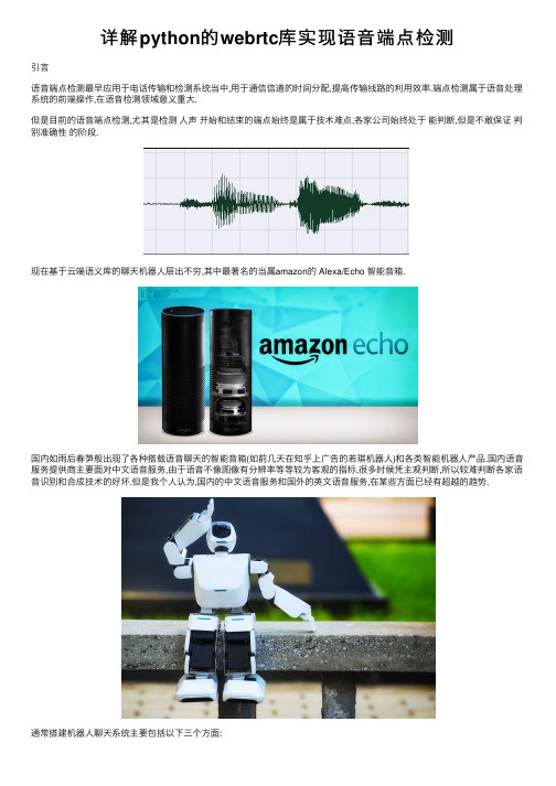
详解python的webrtc库实现语⾳端点检测引⾔语⾳端点检测最早应⽤于电话传输和检测系统当中,⽤于通信信道的时间分配,提⾼传输线路的利⽤效率.端点检测属于语⾳处理系统的前端操作,在语⾳检测领域意义重⼤.但是⽬前的语⾳端点检测,尤其是检测⼈声开始和结束的端点始终是属于技术难点,各家公司始终处于能判断,但是不敢保证判别准确性的阶段.现在基于云端语义库的聊天机器⼈层出不穷,其中最著名的当属amazon的 Alexa/Echo 智能⾳箱.国内如⾬后春笋般出现了各种搭载语⾳聊天的智能⾳箱(如前⼏天在知乎上⼴告的若琪机器⼈)和各类智能机器⼈产品.国内语⾳服务提供商主要⾯对中⽂语⾳服务,由于语⾳不像图像有分辨率等等较为客观的指标,很多时候凭主观判断,所以较难判断各家语⾳识别和合成技术的好坏.但是我个⼈认为,国内的中⽂语⾳服务和国外的英⽂语⾳服务,在某些⽅⾯已经有超越的趋势.通常搭建机器⼈聊天系统主要包括以下三个⽅⾯:1. 语⾳转⽂字(ASR/STT)2. 语义内容(NLU/NLP)3. ⽂字转语⾳(TTS)语⾳转⽂字(ASR/STT)在将语⾳传给云端API之前,是本地前端的语⾳采集,这部分主要包括如下⼏个⽅⾯:1. 麦克风降噪2. 声源定位3. 回声消除4. 唤醒词5. 语⾳端点检测6. ⾳频格式压缩python 端点检测由于实际应⽤中,单纯依靠能量检测特征检测等⽅法很难判断⼈声说话的起始点,所以市⾯上⼤多数的语⾳产品都是使⽤唤醒词判断语⾳起始.另外加上声⾳回路,还可以做语⾳打断.这样的交互⽅式可能有些傻,每次必须喊⼀下唤醒词才能继续聊天.这种⽅式聊多了,个⼈感觉会嘴巴疼:-O .现在github上有snowboy唤醒词的开源库,⼤家可以登录snowboy官⽹训练⾃⼰的唤醒词模型.1. Kitt-AI : Snowboy2. Sensory : Sensory考虑到⽤唤醒词嘴巴会累,所以⼤致调研了⼀下,Python拥有丰富的库,直接import就能⾷⽤.这种⽅式容易受强噪声⼲扰,适合⼀个⼈在家玩玩.1. pyaudio: pip install pyaudio 可以从设备节点读取原始⾳频流数据,⾳频编码是PCM格式;2. webrtcvad: pip install webrtcvad 检测判断⼀组语⾳数据是否为空语⾳;当检测到持续时间长度 T1 vad检测都有语⾳活动,可以判定为语⾳起始;当检测到持续时间长度 T2 vad检测都没有有语⾳活动,可以判定为语⾳结束;完整程序代码可以从我的下载程序很简单,相信看⼀会⼉就明⽩了'''Requirements:+ pyaudio - `pip install pyaudio`+ py-webrtcvad - `pip install webrtcvad`'''import webrtcvadimport collectionsimport sysimport signalimport pyaudiofrom array import arrayfrom struct import packimport waveimport timeFORMAT = pyaudio.paInt16CHANNELS = 1RATE = 16000CHUNK_DURATION_MS = 30 # supports 10, 20 and 30 (ms)PADDING_DURATION_MS = 1500 # 1 sec jugementCHUNK_SIZE = int(RATE CHUNK_DURATION_MS / 1000) # chunk to readCHUNK_BYTES = CHUNK_SIZE 2 # 16bit = 2 bytes, PCMNUM_PADDING_CHUNKS = int(PADDING_DURATION_MS / CHUNK_DURATION_MS)# NUM_WINDOW_CHUNKS = int(240 / CHUNK_DURATION_MS)NUM_WINDOW_CHUNKS = int(400 / CHUNK_DURATION_MS) # 400 ms/ 30ms geNUM_WINDOW_CHUNKS_END = NUM_WINDOW_CHUNKS 2START_OFFSET = int(NUM_WINDOW_CHUNKS CHUNK_DURATION_MS 0.5 RATE)vad = webrtcvad.Vad(1)pa = pyaudio.PyAudio()stream = pa.open(format=FORMAT,channels=CHANNELS,rate=RATE,input=True,start=False,# input_device_index=2,frames_per_buffer=CHUNK_SIZE)got_a_sentence = Falseleave = Falsedef handle_int(sig, chunk):global leave, got_a_sentenceleave = Truegot_a_sentence = Truedef record_to_file(path, data, sample_width):"Records from the microphone and outputs the resulting data to 'path'" # sample_width, data = record()data = pack('<' + ('h' len(data)), data)wf = wave.open(path, 'wb')wf.setnchannels(1)wf.setsampwidth(sample_width)wf.setframerate(RATE)wf.writeframes(data)wf.close()def normalize(snd_data):"Average the volume out"MAXIMUM = 32767 # 16384times = float(MAXIMUM) / max(abs(i) for i in snd_data)r = array('h')for i in snd_data:r.append(int(i times))return rsignal.signal(signal.SIGINT, handle_int)while not leave:ring_buffer = collections.deque(maxlen=NUM_PADDING_CHUNKS) triggered = Falsevoiced_frames = []ring_buffer_flags = [0] NUM_WINDOW_CHUNKSring_buffer_index = 0ring_buffer_flags_end = [0] NUM_WINDOW_CHUNKS_ENDring_buffer_index_end = 0buffer_in = ''# WangSraw_data = array('h')index = 0start_point = 0StartTime = time.time()print(" recording: ")stream.start_stream()while not got_a_sentence and not leave:chunk = stream.read(CHUNK_SIZE)# add WangSraw_data.extend(array('h', chunk))index += CHUNK_SIZETimeUse = time.time() - StartTimeactive = vad.is_speech(chunk, RATE)sys.stdout.write('1' if active else '_')ring_buffer_flags[ring_buffer_index] = 1 if active else 0ring_buffer_index += 1ring_buffer_index %= NUM_WINDOW_CHUNKSring_buffer_flags_end[ring_buffer_index_end] = 1 if active else 0ring_buffer_index_end += 1ring_buffer_index_end %= NUM_WINDOW_CHUNKS_END# start point detectionif not triggered:ring_buffer.append(chunk)num_voiced = sum(ring_buffer_flags)if num_voiced > 0.8 NUM_WINDOW_CHUNKS:sys.stdout.write(' Open ')triggered = Truestart_point = index - CHUNK_SIZE 20 # start point# voiced_frames.extend(ring_buffer)ring_buffer.clear()# end point detectionelse:# voiced_frames.append(chunk)ring_buffer.append(chunk)num_unvoiced = NUM_WINDOW_CHUNKS_END - sum(ring_buffer_flags_end)if num_unvoiced > 0.90 NUM_WINDOW_CHUNKS_END or TimeUse > 10:sys.stdout.write(' Close ')triggered = Falsegot_a_sentence = Truesys.stdout.flush()sys.stdout.write('\n')# data = b''.join(voiced_frames)stream.stop_stream()print(" done recording")got_a_sentence = False# write to fileraw_data.reverse()for index in range(start_point):raw_data.pop()raw_data.reverse()raw_data = normalize(raw_data)record_to_file("recording.wav", raw_data, 2)leave = Truestream.close()程序运⾏⽅式sudo python vad.py以上就是本⽂的全部内容,希望对⼤家的学习有所帮助,也希望⼤家多多⽀持。
《基于深度学习的语音端点检测》范文

《基于深度学习的语音端点检测》篇一一、引言随着人工智能技术的不断发展,语音信号处理在众多领域中得到了广泛的应用。
其中,语音端点检测(Voice Activity Detection, VAD)是语音信号处理中的一个重要环节。
它主要用于区分语音信号中的语音段和非语音段,为后续的语音识别、语音合成等任务提供有效的预处理。
传统的语音端点检测方法往往依赖于阈值设定和特征提取,但这些方法往往容易受到噪声和环境因素的影响,导致误检和漏检。
近年来,深度学习技术的崛起为语音端点检测提供了新的解决方案。
本文将探讨基于深度学习的语音端点检测方法,以提高检测质量和鲁棒性。
二、相关工作传统的语音端点检测方法主要基于阈值设定和特征提取。
这些方法通常依赖于预先定义的阈值和特征,如短时能量、过零率等。
然而,这些方法在噪声环境下性能较差,容易受到各种干扰因素的影响。
近年来,深度学习技术在语音识别、语音合成等领域取得了显著的成果。
因此,将深度学习应用于语音端点检测已成为一个研究热点。
三、基于深度学习的语音端点检测方法本文提出一种基于深度学习的语音端点检测方法。
该方法利用循环神经网络(RNN)和卷积神经网络(CNN)的优点,构建一个端到端的模型,实现对语音信号的实时检测。
1. 数据预处理:首先对原始语音信号进行预处理,包括归一化、分帧等操作,以便于后续的模型训练。
2. 模型构建:构建一个基于RNN和CNN的深度学习模型。
RNN用于捕捉语音信号的时间依赖性,CNN用于提取局部特征。
通过将RNN和CNN进行融合,可以实现对语音信号的时空特征提取。
3. 训练与优化:使用大量的语音数据对模型进行训练,并采用适当的损失函数和优化算法来优化模型的性能。
此外,为了进一步提高模型的泛化能力,还可以采用数据增强等技术对训练数据进行扩展。
4. 实时检测:将训练好的模型应用于实时语音信号中,实现对语音段的实时检测。
通过设置合适的阈值,可以有效地区分出语音段和非语音段。
语音端点检测方法研究
语音端点检测方法研究1沈红丽,曾毓敏,李平,王鹏南京师范大学物理科学与技术学院,南京(210097)E-mail:orange.2009@摘要: 端点检测是语音识别中的一个重要环节。
有效的端点检测技术不仅能减少系统的处理时间,增强系统处理的实时性,而且能排除无声段的噪声干扰,增强后续过程的识别性。
可以说,语音信号的端点检测至今天为止仍是有待进一步深入的研究课题.鉴于此,本文介绍了语音端点算法的基本研究现状,接着讨论并比较了语音信号端点检测的方法,分析了各种方法的原理及优缺点,如经典的基于短时能量和过零率的检测方法,基于频带方差的检测方法,基于熵的检测方法,基于倒谱距离的检测方法等.并基于这些方法的分析,对端点检测方法做了进行了总结和展望,对语音信号的端点检测的进一步研究具有深远的意义。
关键词:语音信号;端点检测;噪声中图分类号:TP206. 11. 引言语音信号处理中的端点检测技术,是指从包含语音的一段信号中确定出语音信号的起始点及结束点。
语音信号的端点检测是进行其它语音信号处理(如语音识别、讲话人识别等)重要且关键的第一步. 研究表明[1],即使在安静的环境中,语音识别系统一半以上的识别错误来自端点检测器。
因此,作为语音识别系统的第一步,端点检测的关键性不容忽视,尤其是噪声环境下语音的端点检测,它的准确性很大程度上直接影响着后续的工作能否有效进行。
确定语音信号的起止点, 从而减小语音信号处理过程中的计算量, 是众多语音信号处理领域中一个基本而且重要的问题。
有效的端点检测技术不仅能减少系统的处理时间,增强系统处理的实时性,而且能排除无声段的噪声干扰,增强后续过程的识别性。
可以说,语音信号的端点检测至今天为止仍是有待进一步深入的研究课题。
2. 语音端点检测主要方法和分析在很长一段时间里,语音端点检测算法主要是依据语音信号的时域特性[2].其采用的主要参数有短时能量、短时平均过零率等,即通常说的基于能量的端点检测方法。
《基于深度学习的语音端点检测》范文
《基于深度学习的语音端点检测》篇一一、引言随着人工智能技术的快速发展,语音识别技术得到了广泛的应用。
在语音识别系统中,语音端点检测(Voice Activity Detection,VAD)是一个重要的预处理步骤,它能够有效地将语音信号中的非语音部分剔除,从而提高语音识别的准确性和效率。
传统的语音端点检测方法往往基于简单的统计特征或者固定阈值来进行判断,但是这种方法容易受到环境噪声的干扰,无法满足实际应用的需求。
近年来,深度学习技术的发展为语音端点检测提供了新的解决方案。
本文旨在探讨基于深度学习的语音端点检测方法,以提高其准确性和鲁棒性。
二、相关工作传统的语音端点检测方法通常使用短时能量、过零率等特征来判断语音的起点和终点。
这些方法在较为简单的环境中效果尚可,但面对复杂的背景噪声、语音环境变化等情况时,其性能会显著下降。
近年来,深度学习技术在语音识别、语音合成等领域取得了显著的成果。
因此,越来越多的研究者开始探索基于深度学习的语音端点检测方法。
这些方法能够自动学习并提取更丰富的语音特征,从而提高对噪声的鲁棒性。
三、基于深度学习的语音端点检测方法本文提出了一种基于深度学习的语音端点检测方法。
该方法使用循环神经网络(RNN)和卷积神经网络(CNN)进行特征提取和分类。
首先,将原始的音频信号进行预处理,提取出短时段的音频帧作为输入数据。
然后,利用CNN对每个音频帧进行特征提取,获取音频的时频特征。
接着,使用RNN对时频特征进行序列建模,以便捕捉音频中的连续信息。
最后,通过一个全连接层进行分类,判断该段音频是否为语音。
具体实现中,我们选择了两种常用的神经网络结构进行实验对比:LSTM-RNN和GRU-RNN。
LSTM-RNN具有更强的记忆能力,适合处理长序列数据;而GRU-RNN则具有更少的参数和更快的训练速度。
在特征提取方面,我们尝试了多种不同的CNN 结构,包括一维卷积神经网络和二维卷积神经网络等。
语音端点检测
语音信号的最基本组成单位是音素。音素可分成浊音和清音两大类。如果将不存在语音而只有背景噪声的情况成为“无声”,那么音素可分成“无声”、“浊音”和“清音”三类。在短时分析的基础上可判断一短段语音属于哪一类。如果是浊语音段,还可测定它的另一些重要参数,如基音和共振峰等。
2.2 语音信号分析
语音信号处理包括语音识别、语音合成、语音编码、说话人识别等方面,但是其前提和基础是对语音信号进行分析。只有将语音信号分析成表示其本质特性的参数,才有可能利用这些参数进行高效的语音通信,以及建立用于识别的模板或知识库。而且,语音识别率的高低,语音合成的音质好坏,都取决于对语音信号分析的准确性和精度
第三章,从每一种算法的方程式入手,以原理简便、运算量小等方面为标准,通过大量的文献调研与实际研究,本课主题要研究语音起点和终点的检测,以短时能量和短时过零率相结合的双门限语音端点检测算法以及倒谱分析和谱熵技术等进行语音端点检测,并分析各算法在低信噪比和高信噪比条件下的检测效果进行对比。
对这种信号进行Matlab进行编程,对于不同信噪比的声音片段,最后用前后的噪声信号进行对比以得出结论
1.2 语音端点检测现状
作为一个完整的语音识别系统,其最终实现及使用的效果不仅仅限于识别的算法,许多相关因素都直接影响着应用系统的成功与否。语音识别的对象是语音信号,端点检测的目的就是在复杂的应用环境下的信号流中分辨出语音信号和非语音信号,并确定语音信号的开始及结束。一般的信号流都存在一定的背景声,而语音识别的模型都是基于语音信号训练的,语音信号和语音模型进行模式匹配才有意义。因此从信号流中检测出语音信号是语音识别的必要的预处理过程[2]。
重点(端点检测)

在设计一个成功的端点检测模块时,会遇到下列一些实际困难:⑴信号取样时,由于电平的变化,难于设置对各次试验都适用的阀值。
⑵在发音时,人的咂嘴声或其他某些杂音会使语音波形产生一个很小的尖峰,并可能超过所设计的门限值。
此外,人呼吸时的气流也会产生电平较高的噪声。
⑶取样数据中,有时存在突发性干扰,使短时参数变得很大,持续很短时间后又恢复为寂静特性。
应该将其计入寂静段中。
⑷弱摩擦音时或终点处是鼻音时,语音的特性与噪声极为接近,其中鼻韵往往还拖得很长。
⑸如果输入信号中有50Hz工频干扰或者A/D变换点的工作点偏移时,用短时过零率区分无声和清音就变的不可靠。
一种解决方法是算出每一帧的直流分量予以减除,但是这无疑加大了运算量,不利于端点检测算法的实时执行;另一种解决方法是采用一个修正短时参数,它是一帧语音波形穿越某个非零电平的次数,可以恰当地设置参数为一个接近于零的值,使得过零率对于清音仍具有很高的值,而对于无声段值却很低。
但事实上,由于无声段以及各种清音的电平分布情况变化很大,在有些情况下,二者的幅度甚至可以相比拟,这给这个参数的选取带来了极大的困难[5]。
由上可见,一个优秀的端点检测算法应该能满足:⑴门限值应该可以对背景噪声的变化有一定的适应。
⑵将短时冲击噪声和人的咂嘴等瞬间超过门限值的信号纳入无声段而不是有声段。
⑶对于爆破音的寂静段,应将其纳入语音的范围而不是无声段。
⑷应该尽可能避免在检测中丢失鼻韵和弱摩擦音等与噪声特性相似、短时参数较少的语音。
⑸应该避免使用过零率作为判决标准而带来的负面影响。
在做本课题时,端点检测方法是将语音信号的短时能量与过零率相结合加以判断的。
但这种端点检测算法如果运用不好,将会发生漏检或虚检的情况。
语音信号大致可以分为浊音和清音两部分,在语音激活期的开始往往是电平较低的清音,当背景噪声较大时,清音电平与噪声电平相差无几。
采用传统的语音端点检测方法很容易造成语音激活的漏检。
而语音信号的清音段,对于语音的质量起着非常重要的作用。
基于短时自相关及过零率的语音端点检测算法
基于短时自相关及过零率的语音端点检测算
法
语音端点检测是计算机语音处理领域的一种常见应用,它主要用于语音识别、拼写校正以及声纹分析等语音处理技术中。
基于短时自相关(Short-Time Auto/orrelation, STAC)和过零率(Zero-Crossing Rate, ZCR)的语音端点检测算法是当前检测语音端点所使用的一种常用方法。
通常情况下,该算法的实现步骤如下:首先,将语音信号拆分为多小片段,每块片段的长度一般以毫秒为单位(通常取20ms),并将片段之间用某种滤波器连接;接着计算每块片段的自相关系数,并在计算结果中检测端点;最后,计算每个片段的ZCR,用相邻两个片段之间的ZCR变化来确定语音端点,其中该变化值还可以决定端点的类型—开始点或结束点。
检测完语音端点后,即可实现对语音信号的分割及识别。
现有的STAC-ZCR算法效果较为理想,其特点是计算量小、易于实现,因此深受人们的欢迎并发展至今。
实验一语音信号端点检测
实验一语音信号端点检测一、 实验目的1.学会MATLAB 的使用,掌握MATLAB 的程序设计方法;2.掌握语音处理的基本概念、基本理论和基本方法;3.掌握基于MATLAB 编程实现带噪语音信号端点检测;4.学会用MATLAB 对信号进行分析和处理。
5. 学会利用短时过零率和短时能量,对语音信号的端点进行检测。
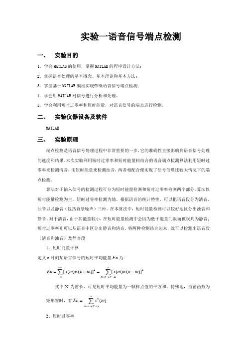
二、 实验仪器设备及软件MATLAB三、 实验原理端点检测是语音信号处理过程中非常重要的一步,它的准确性直接影响到语音信号处理的速度和结果。
本次实验利用短时过零率和短时能量相结合的语音端点检测算法利用短时过零率来检测清音,用短时能量来检测浊音,两者相配合便实现了信号信噪比较大情况下的端点检测。
算法对于输入信号的检测过程可分为短时能量检测和短时过零率检测两个部分。
算法以短时能量检测为主,短时过零率检测为辅。
根据语音的统计特性,可以把语音段分为清音、浊音以及静音(包括背景噪声)三种。
在本算法中,短时能量检测可以较好地区分出浊音和静音。
对于清音,由于其能量较小,在短时能量检测中会因为低于能量门限而被误判为静音;短时过零率则可以从语音中区分出静音和清音。
将两种检测结合起来,就可以检测出语音段(清音和浊音)及静音段1、短时能量计算定义n 时刻某语言信号的短时平均能量En 为:∑∑--=+∞∞--=-=n N n m m n w m x m n w m x En )1(22)]()([)]()([式中N 为窗长,可见短时平均能量为一帧样点值的平方和。
特殊地,当窗函数为矩形窗时,有∑--==n N n m m x En )1(2)(2、短时过零率过零就是指信号通过零值。
过零率就是每秒内信号值通过零值的次数。
对于离散时间序列,过零则是指序列取样值改变符号,过零率则是每个样本的改变符号的次数。
对于语音信号,则是指在一帧语音中语音信号波形穿过横轴(零电平)的次数。
可以用相邻两个取样改变符号的次数来计算。
如果窗的起点是n=0,短时过零率Z 为波形穿过横轴(零电平)的次数|))1(())((|2110∑-=--=N n w w n S Sgn n S Sgn Z {00,1,1)sgn(≥<-=x x x短时过零可以看作信号频率的简单度量浊音的短时平均幅度最大,无声的短时平均幅度最小,清音的短时过零率最大,无声居中,浊音的短时过零率最小。
语音端点检测
1.3 相关工作
随着生活品质的不断提高,对声控产品,在不同的声控产品语音识别系统中,有效准确地确定语音段端点不仅能使处理时间减到最小,而且能排除无声段的噪声干扰,从而使识别系统具有良好的性能。
随着语音识 别应用的发展,越来越多系统将打断功能作为一种方便有效的应用模式,而打断功能又直接依赖端点检测。端点检测对打断功能的影响发生在判断语音/非语音的过 程出现错误时。表现在过于敏感的端点检测产生的语音信号的误警将产生错误的打断。例如,提示音被很强的背景噪音或其它人的讲话打断,是因为端点检测错误的 将这些信号作为有效语音信号造成的。反之,如果端点检测漏过了事实上的语音部分,而没有检测到语音。系统会表现出没有反应,在用户讲话时还在播放提示音。
通过大量的文献调研与实际研究发现,现有的各种语音信号端点检测技术都存在各自的不足。对于语音信号在低信噪比时的端点检测的研究有待进一步深入研究。当前,语音端点检测技术还远滞于通信技术发展的脚步,在此领域还有很多问题需要研究。
对于强干扰非平稳噪声和快速变化的噪声环境,如何找到更好的端点检测方法是进一步研究的主要方向。提取人耳听觉特性可以更加有效地区分语音和噪声,从而更加准确的检测语音端点。预先未知噪声统计信息条件下的语音端点检测算法已经出现,但仍出去萌芽阶段。虽然预先未知噪声统计信息条件下的端点检测是未来语音端点检测技术的发展方向,但在理论方法和技术参数等方面还有待进一步突破[17]。
目前,语音技术正进入一个相对成熟点,很多厂商和研究机构有了语音技术在输入和控制上令人鼓舞的演示,输入的硬件和软件平台环境也日益向理想化迈进,但语音技术比起人类的听觉能力来还相差甚远,其应用也才刚刚开始,进一步规范和建设语音输入的硬件通道、软件基本引擎和平台,使语音技术能集成到需要语音功能的大量软件中去。而且语音产业需要更加开放的环境,使有兴趣和实力的企业都能加入到这方面的研究和开发中,逐步改变。随着声控电子产品的不断研发,语音识别技术在开发和研究上还有大量的工作需要做。
一种噪声环境的语音端点检测方法
f r a c e c n p i t e e t n o m n e i s e h e d o n t ci . n p d o
Ke r s t — eu nya a s ; u bn ae e s a( B ;n p it eet n ywod :i f q ec l i S b a dB sdC pt lS C)e d on dtc o me r nys r i
C m ue n ier ga d p l ain 计 算机 工程 与应用 o p t E gn ei A p i t s r n n c o
一
种噪声环境 的语音端 点检测 方法
帛, 冯新喜 , 邱浪波 b NG Bo F NG Xix, U a g o
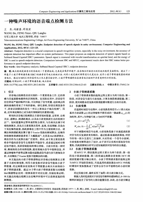
常 用的语 音端 点检测算法 主要 有短 时能 量 、 零率 、 过 自相 关法、 谱熵 法 、 谱距 离法 , 倒 以及 由小 波变换 派生 出的检测 方 法 时能量 和过零 率通常 配合使 用 , 自相关 法属 于时 。。短 与 域检 测算 法 , 其优点主要 是算法简单 、 直观 , 容易理解 , 但是 由 于 其抗噪 性较差 , 因此很 难在工 程 中作为主要 检测 方法 。谱 熵法 和倒 谱距离法 属于基 于 F uir o r 变换 的频域 算法 , 噪性 e 抗 和检 测效 果都较 前者 有 了大幅提 高 , 其是 Me倒 谱算 法 , 尤 l
摘
要 : 点检 测是 语音识别 系统 的一 个重要 组成 , 其是 在噪声环境 中, 端 尤 其准确性对语音识别 系统性 能有 直接 影响。提 出了一
种基 于 小波子 带倒 谱 系数 (B ) S C 的语音信 号端点检 测方法 , 利用 小波变换 对频 带进行 尺度划分 , 采用 小波子带倒谱 能量检 测语 音端点。通过与 MF C的仿真对 比以及 大量实验 分析 , C 小波子 带倒谱特征在语音 端点检 测申具有 更好 的识别性能。 关键词 : 时频分析 ; 小波子带倒谱 系数 ; 端点检 测
《语音信号处理》实验1-端点检测

华南理工大学《语音信号处理》实验报告实验名称:端点检测姓名:学号:班级:10级电信5班日期:2013年5 月9日1.实验目的1.语音信号端点检测技术其目的就是从包含语音的一段信号中准确地确定语音的起始点和终止点,区分语音和非语音信号,它是语音处理技术中的一个重要方面。
本实验的目的就是要掌握基于MATLAB编程实现带噪语音信号端点检测,利用MATLAB对信号进行分析和处理,学会利用短时过零率和短时能量,对语音信号的端点进行检测。
2. 实验原理1、短时能量语音和噪声的区别可以体现在它们的能量上,语音段的能量比噪声段能量大,语音段的能量是噪声段能量叠加语音声波能量的和。
在信噪比很高时,那么只要计算输入信号的短时能量或短时平均幅度就能够把语音段和噪声背景区分开。
这是仅基于短时能量的端点检测方法。
信号{x(n)}的短时能量定义为:语音信号的短时平均幅度定义为:其中w(n)为窗函数。
2、短时平均过零率短时过零表示一帧语音信号波形穿过横轴(零电平)的次数。
过零分析是语音时域分析中最简单的一种。
对于连续语音信号,过零意味着时域波形通过时间轴;而对于离散信号,如果相邻的取样值的改变符号称为过零。
过零率就是样本改变符号次数。
信号{x(n)}的短时平均过零率定义为:式中,sgn为符号函数,即:过零率有两类重要的应用:第一,用于粗略地描述信号的频谱特性;第二,用于判别清音和浊音、有话和无话。
从上面提到的定义出发计算过零率容易受低频干扰,特别是50Hz交流干扰的影响。
解决这个问题的办法,一个是做高通滤波器或带通滤波,减小随机噪声的影响;另一个有效方法是对上述定义做一点修改,设一个门限T,将过零率的含义修改为跨过正负门限。
于是,有定义:3、检测方法利用过零率检测清音,用短时能量检测浊音,两者配合。
首先为短时能量和过零率分别确定两个门限,一个是较低的门限数值较小,对信号的变化比较敏感,很容易超过;另一个是比较高的门限,数值较大。
语音信号处理-端点检测

A noise robust endpoint detection algorithm for whispered speech based on EmpiricalMode Decomposition and entropyXue-Dan Tan Dept. of Phys. Sci. and Tech.Soochow UniversitySuzhou, Chinatanxuedan@He-Ming ZhaoDept. of ElectronSoochow UniversitySuzhou, ChinaJi-Hua Gu Dept. of Phys. Sci. and Tech Soochow UniversitySuzhou, ChinaZhi TaoDept. of Phys. Sci. and Tech Soochow UniversitySuzhou, Chinataoz@Abstract—This paper proposes a novel endpoint detection algorithm to improve the speech detection performance in noisy environments. In the proposed algorithm, Empirical Mode Decomposition is introduced to improve the performance of voice activity detector based on spectral entropy. We have evaluated system performance under noisy environments using a whispered database and NOISEX-92 Database. Experimental results indicate that our approach performs well in the degraded environment.Keywords-endpoint detection; whispered speech; Empirical Mode Decomposition; entropyI.I NTRODUCTIONEndpoint detection is used to distinguish speech from other waveforms. In many cases, endpoint detection has very board applications and plays an important part in speech and hearing, such as speech coding, speech recognition and speech enhancement. Many endpoint detectors algorithms have been proposed which are based on features of short-time signal energy, the high band energy and zero-crossing rate. However, these features do not work well under whispered conditions.Whisper is a natural form of speech that one uses for a variety of reasons. For example, individuals often communicate in environments where normal speech is inappropriate, while aphonic individuals may not be able to produce normal speech [1]. The mechanism of whisper production is different from normal speech. In normal speech, voiced sounds are produced by quasi-periodic excitation pulses. However, whispered speech is completely noise excited, with 20dB lower power than its equivalent voiced speech [2]. The spectrum of whispers also rolls off under 500Hz [3] due to an introduced spectral zero [4] and is typically flatter than the voiced spectrum between 500 and 2000 Hz [5].Because of no vocal fold vibration and low energy as well as noise-like, whispered speech is more difficult to detect than normal speech, especially under noisy environments.In [6], a robust VAD method based on spectral entropy was proposed. This method has shown a high detection accuracy compared with the conventional methods. Motivated by the feature in [6], an improved method in [7] was developed to identify whispered speech segments accurately. Both [6] and [7] are well suited for endpoint detection in stationary noise. However, most of noises are non-stationary. Each type of noise has its special distribution on the spectrum, and all of them are quite different from that of speech signal. The two methods above would become less reliable in non-stationary noise like Babble noise.In this paper, we focus on the method in [7] based on the improved spectral entropy, and incorporate Empirical Mode Decomposition (EMD) to improve the robustness of endpoint detection. EMD, introduced by Dr. Norden Huang in 1998 [8], is a powerful analytical method for non-linear and non-stationary signals. We use EMD to decompose whispered speech signal self-adaptively and locally. Some of the resulting IMFs are less noisy than the original signal, so we extract entropy-based feature from these IMFs and the experiments show that the proposed feature is superior to the entropy extracted from original whispered speech directly and the proposed method outperforms [7], especially under non-stationary background noise.The rest of this paper is organized as follows: in section 2, the basics of EMD is considered, then in section 3, the method in [7] is described, in section 4, the proposed method is introduced, and the experiments are shown in section 5 and finally, the conclusions are given in section 6.II.E MPIRICAL M ODE D ECOMPOSITION M ETHOD The EMD decomposes a given signal x(n) into a series of IMFs through an iterative process: each one with a distinct time scale [8]. The decomposition is based on the local time scale of x(n), and yields adaptive basis functions. The EMD can be seen as a type of wavelet decomposition whose sub-bands are built up as needful to separate the different components of x(n). Each IMF replaces the signal details, at a certain scale or frequency band [9]. The EMD picks out the highest frequency oscillation that remains in x(n). By definition, an IMF satisfies two conditions:1)The number of extremes and the number of zerocrossings may differ by no more than one.University Natural Science Research Project of Jiangsu Province (Grant No. 09KJD510005).Third International Symposium on Intelligent Information Technology and Security Informatics2) The average value of the envelope defined by the localmaxima, and the envelope defined by the local minima, is zero. Thus, locally, each IMF contains lower frequency oscillations than the just extracted one. The EMD does not use a pre-determined filter or a wavelet function, and is a fully data-driven method [8].For a given x(n), the algorithm of the EMD can be summarized as follows:1) Find all the points of the local maximum and all thepoints of the local minimum in the signal. 2) Create the upper envelope by a spline interpolation ofthe local maximum and the lower envelope by a spline interpolation of the local minimum of the input signal. 3) Calculate the mean of the upper envelope and thelower envelope. 4) Subtract the envelope’s mean signal from the inputsignal to yield the residual. 5) Iterate on the residual until it satisfies the “stop”criterion, The ‘stop’ criterion functions to check if the residual from Step 4 is an IMF or not. 6) Repeat the sifting process from Step 1 to Step 5 manytimes with the residue as the input signal so that all the IMFs can be extracted from the signal. After the EMD, the original input signal x(n) can be expressed as follows:1()()()nini x n c n r ¦n (1)III. S PECTRAL E NTROPYIn [7], the whispered speech is segmented into frames and pre-filtered by a high-pass filter setting of 500 Hz. Each frame is evenly divided into 4 sub-frames. For each sub-band, assuming X(k) is the wide-band spectrogram of speech frame x(n):12()()exp()Nn j nk X k x n NS ¦, k =1,}, N ; N =128 (2)Define s(k) as its power spectrum2()()s k X k (3)And E f denotes its energy1()Mf k E s k ¦, k =1,}, M ; M =64 (4)p(k) is the probability densities in frequency domain and can be written as()()fs k p k E (5)Thus the entropy for each sub-frame speech signal is defined as1()log ()Mk H p k p k ¦ (6)And the spectral entropy for the frame can then be calculated as the average of four sub-frames.IV. A N ENDPOINT DETECTION ALGORITHM FOR WHISPEREDSPEECH USING EMD AND SPECTRAL ENTROPY A speech signal is first decomposed into often finite IMFs by the EMD, as shown in (1). During the decomposition of EMD, on each little period of time, IMFs with the minimal scale are obtained first, then are IMFs with large scales, in the end is the IMF with the maximal scale. Theoretically, an IMF is a mono-component function, and is generated orderly according to the local time scales of the components. It turns out that EMD acts essentially as a dyadic filter bank resembling those involved in wavelet decompositions [9]. The whispered speech signal and the first six IMFs out of twelveand their spectrums are shown in Fig.1.Figure 1. The EMD of whispered speech “chuai” (the first six IMFs out oftwelve) and spectrumsIt is observed that the resulting IMFs are the different frequency parts of the signal. And compared with the original whispered speech signal, each spectrum of IMFs, especially the smaller-scale IMFs, is less noisy. Besides, speech has the AM-FM characteristics while noise signal does not, and the processing of EMD can meet these characteristics. As a result, whispered parts of IMFs are more stable than the noisy parts, namely, entropy values of whispered part are larger than the ones of noisy parts which is shown in Fig.2.Figure 2. The EMD of whispered speech “chuai” (the first six IMFs outof twelve) and entropy curvesThe larger scales have very low amplitudes, which are very small compared to the other IMFs, and thus it is not necessary to calculate theses posterior IMFs. This helps to reduce the computing time.The algorithm can be summarized as follows:1) Decompose the whispered speech signal with theEMD. 2) Choose the i -th IMF component, where i = 0, 1,}, I . 3) Weight the i -th IMF component by the Hammingwindow.Z (n )=0.54 0.46cos (2*S n /N ), n = 0, 1,} ,N 1 (7) where N is the frame length.4) Compute H(i ,j), which is the spectral entropy of the j -th frame of the i -th IMF component. 5) The final estimate is given by1()(,)Ii E j H i j ¦, j =1, 2,}, J (8)where J is the frame number of each IMF component.V.E XPERIMENT AND RESULTSThe whispered speech database used in the experiments here is Whisper_N Database (the whispered speech database constructed by the researchers of Nanjing University [10]) with a 2~10dB signal-to-noise ratio (SNR) from different male and female speakers. The noise signals used in the simulation include 3 kinds of noise (Babble, Volvo and F16) of NOISEX-92 Database. The whispered speech and various noise signals are mixed at 6 different SNRs (0dB, 5dB, 10dB, 15dB, 20dB and 25dB) to simulate the real noise environments. And we use a method based on energy and zero-crossing rate (method 1)and the method in [7] (method 2) for comparison with the proposed method (method 3). In our experiments, FFT is 512 points and window length is 256 samples with a window shift of 80 samples.A. Feature ComparisonFig.3 shows the features of three endpoint detection methods for clean whispered speech. One can notice that the discriminability of the proposed feature is obviously better than the others.Fig.4, Fig.5 and Fig.6 include the feature curves of the three methods above under Babble, Volvo and F16 noisebackgrounds respectively and SNR=10dB.(a) Clean whispered speech (b) Babble noise(c) Volvo noise (d) F16 noiseFigure 3. Various feature curves for whispered speech “chuai” indifferent types of noise at 10 dB SNRFrom the last figures, it is found that the introduction of EMD in method 3 almost makes the curves of noise become fairly flatter than the entropy in method 2, and the speech distributions in method 3 are more evident than others under the same SNR condition. It is obvious that the thresholds are easy to be tuned consistently for different noise signals. B. Endpoint Detection ExperimentsIn this experiment, we process 205 whispered speech samples from Whisper_N Database by the three methods above. The correct segmentation rates of clean whispered speech are showed in Table ȱ.TABLE I. CORRECT SEGMENTATION RATES OF CLEAN WHISPEREDSPEECH (%)Method 1 Method 2 Method 3Start point90.7317 93.1707 99.0244 End point48.4634 70.2439 83.90241)The accurate rates of both start point detection andend point detection obtained by method 3 are higher than others’. 2) All the accurate rates of start point detection are betterthan that of end point detection. Because the end of whispered speech signal is weaker than the start, the three methods above deteriorate at the detection of end points. The segmentation results obtained by the three methods above with different types and levels of noise are shown in Fig. 4, Fig. 5 and Fig. 6.(a) Start point(b) End pointFigure 4. Segmentation rates in Babble noise(a) Start point(b) End pointFigure 5. Segmentation rates in Volvo noise(a) Start point(b) End pointFigure 6. Segmentation rates in F16 noiseThe figure results prove that method 3 has an overall better performance than others in all SNRs and all the noise types used here. It can be noticed that method outperforms method 1, for example, Fig.5 and Fig.6 (b). Method 2 becomes useless in the presence of the non-stationary noises, which is particularly noticeable in Fig.4 (b) and Fig.6 (b). Thus we can see robustness of our approach under noisy conditions.VI. C ONCLUSIONSIn this paper, we presented a new method based on EMD and spectral entropy for whispered speech detection. The EMD decomposes the signals self-adaptively and locally. The resulting IMFs provide the local information, which is vital to the non-stationary signals. We get the entropy features from smaller scale IMF components. The proposed method benefits from the advantages of the EMD and attractive properties of the entropy and gets rid of the background noise to a certain extent. Our experiments show the proposed method can extract the whispered speech better than the method based on energy and zero-crossing rate and the method in [7], especially in noisy environments. However, the main limitation of EMD-based method is that it is computationally expensive. And the next step is to reduce the computational cost of the proposed method, and to enhance the detection rate of end point of our algorithm to be more effective at very low SNR Environment, for example, at 0 dB.R EFERENCES[1] R.W. Morris, M.A. Clements, “ Reconstruction of speech fromwhispers,” J. Medical Engineering & Physics. vol.24, pp.515-520, 2002. [2] Jovicic S.T, Dordevic M.M, “ Acoustic features of whisperedspeech.,”Acustica-acta acustica. 1996, 82:S228.[3] Jovicic S.T, “Formant feature differences between whispered and voicedsustained vowels,” Acustica-acta acustica. vol.84, pp.739-43, 1998. [4] Stevens K.N, Acoustic phonetics. Cambridge, MA: MIT Press.1998.[5] Schwartz MF, “Power spectral density measurements of oral andwhispered speech,” J .Speech Hearing Res. vol.13, pp.445-446, 1970.[6]Jia-lin Shen, Jeil-weih Hung, Lin-shan Lee, “Robust Entropy-basedEndpoint Detection for Speech Recognition in Noisy Environments,”ICSLP. pp.232-235, 1998.[7]Li X.L., Ding H.,Xu B.L., “Entropy-based initial/final segmentation forChinese whispered speech,” Acta Acustica.2005, 30(1), pp.69-75.[8]Norden E Huang, Shen Zheng, “The empirical mode decomposition andthe Hilbert spectrum for nonlinear and non-stationary time series analysis,” J. Proceedings of the Roya1 Society of London, A454, pp.903-995, 1998.[9]Patrick Flandin, Gabriel Rilling, Paulo Goncalves, “Empirical ModeDecomposition As A Filter Bank,” IEEE Signal Processing Letters.pp.112-114, 2004.[10]Yang L.L., Li Y., Xu B.L., “The establishment of a Chinese whisperdatabase and perceptual experiment,” Journal of Nanjing University (Natural Sciences). pp.311-317, vol.41, 2005.。
端点检测

语音信号处理实验一:端点检测姓名:XXX 学号:XXXX 班级:XX一、实验目的:理解语音信号时域特征和倒谱特征求解方法及其应用。
二、实验原理与步骤:任务一:语音端点检测。
语音端点检测就是指从包含语音的一段信号中确定出语音的起始点和结束点。
正确的端点检测对于语音识别和语音编码系统都有重要的意义。
采用双门限比较法的两级判决法,具体如下第一级判决:1. 先根据语音短时能量的轮廓选取一个较高的门限T1,进行一次粗判:语音起止点位于该门限与短时能量包络交点所对应的时间间隔之外(即AB段之外)。
2. 根据背景噪声的平均能量(用平均幅度做做看)确定一个较低的门限T2,并从A点往左、从B点往右搜索,分别找到短时能量包络与门限T2相交的两个点C和D,于是CD段就是用双门限方法根据短时能量所判定的语音段。
第二级判决:以短时平均过零率为标准,从C点往左和从D点往右搜索,找到短时平均过零率低于某个门限T3的两点E和F,这便是语音段的起止点。
门限T3是由背景噪声的平均过零率所确定的。
注意:门限T2,T3都是由背景噪声特性确定的,因此,在进行起止点判决前,T1,T2,T3,三个门限值的确定还应当通过多次实验。
任务二:利用倒谱方法求出自己的基音周期。
三、实验仪器:Cooledit、Matlab软件四、实验代码:取端点流程图一:clc,clear[x,fs,nbits]=wavread('fighting.wav'); %x为0~N-1即1~Nx = x / max(abs(x)); %幅度归一化到[-1,1]%参数设置FrameLen = 240; %帧长,每帧的采样点inc = 80; %帧移对应的点数T1 = 10; %短时能量阈值,语音段T2 = 5; %短时能量阈值,过渡段T3 = 1; %过零率阈值,起止点minsilence = 6; %无声的长度来判断语音是否结束silence = 0; %用于无声的长度计数minlen = 15; %判断是语音的最小长度state = 0; %记录语音段状态0 = 静音,1 = 语音段,2 = 结束段count = 0; %语音序列的长度%计算短时能量shot_engery = sum((abs(enframe(x, FrameLen,inc))).^2, 2);%计算过零率tmp1 = enframe(x(1:end-1), FrameLen,inc);%tmp1为二维数组=帧数*每帧的采样点FrameLentmp2 = enframe(x(2:end) , FrameLen,inc);%signs = (tmp1.*tmp2)<0;%signs为一维数组,符合的置1,否则置0zcr = sum(signs,2);%开始端点检测,找出A,B点for n=1:length(zcr)if state == 0 % 0 = 静音,1 = 可能开始if shot_engery(n) > T1 % 确信进入语音段x1 = max(n-count-1,1); % 记录语音段的起始点state = 2; silence = 0;count = count + 1;elseif shot_engery(n) > T2|| zcr(n) > T3 %只要满足一个条件,可能处于过渡段status = 1;count = count + 1;x2 = max(n-count-1,1);else % 静音状态state = 0; count = 0;endendif state = =2 % 1 = 语音段if shot_engery(n) > T2 % 保持在语音段count = count + 1;elseif zcr(n) > T3 %保持在语音段x3 = max(n-count-1,1);else % 语音将结束silence = silence+1;if silence < minsilence %静音还不够长,尚未结束count = count + 1;elseif count < minlen % 语音段长度太短,认为是噪声 state = 0;silence = 0;count = 0;else % 语音结束state = 3;endendendif state = =3 % 2 = 结束段break;endendx1,x2,x3 %A、C、E坐标x11 = x1 + count -1 %B坐标x22 = x2 + count -1 %D坐标x33 = x3 + count -1 %F坐标%画图subplot(3,1,1)plot(x)axis([1 length(x) -1 1])%标定横纵坐标title('原始语音信号','fontsize',17);xlabel('样点数'); ylabel('Speech');line([x3*inc x3*inc], [-1 1], 'Color', 'red'); %画竖线line([x33*inc x33*inc], [-1 1], 'Color', 'red');subplot(3,1,2)plot(shot_engery);axis([1 length(shot_engery) 0 max(shot_engery)])title('短时能量','fontsize',17);xlabel('帧数'); ylabel('Energy');line([x1 x1], [min(shot_engery),T1], 'Color', 'red'); %画竖线line([x11 x11], [min(shot_engery),T1], 'Color', 'red'); % line([x2 x2], [min(shot_engery),T2], 'Color', 'red'); % line([x22 x22], [min(shot_engery),T2], 'Color', 'red'); % line([1 length(zcr)], [T1,T1], 'Color', 'red', 'linestyle', ':'); %画横线line([1 length(zcr)], [T2,T2], 'Color', 'red', 'linestyle', ':'); %text(x1,-5,'A'); %标写A、B、C、Dtext(x11-5,-5,'B');text(x2-10,-5,'C');text(x22-5,-5,'D');subplot(3,1,3)plot(zcr);axis([1 length(zcr) 0 max(zcr)])title('过零率','fontsize',17);xlabel('帧数'); ylabel('ZCR');line([x3 x3], [min(zcr),max(zcr)], 'Color', 'red'); %画竖线line([x33 x33], [min(zcr),max(zcr)], 'Color', 'red'); %line([1 length(zcr)], [T3,T3], 'Color', 'red', 'linestyle', ':'); %画横线text(x3-10,-3,'E起点'); %标写E、Ftext(x33-40,-3,'F终点');运行结果与分析:x1 = 650,x11 = 734,x2 = 646,x22 = 752,x3 = 643,x33 = 763得出的值x3<x2 <x1 <x11< x22< x33 ,基本符合要求放大放大放大1、主要是学习了一些新的函数。
一种语音信号端点检测的改进方法

中 图分 类 号 :P 9 T 31 文 献标 识 码 : B
An m pr v d M e h d o h ie En o n t ci n I o e t o ft e Vo c dp i tDe e to
GU Ya—q a g, in ZHAO i W U Hu , Bo
( ol eo Eet ncS i c n nier aoa U i rt e neT cnlg , hnsaHua 103 hn ) C l g f lc oi ce eadE g e,N t nl nv syo D f c eh o y C agh nn4 07 ,C ia e r n n i ei f e o
第2卷 第5 7 期
文章编号 :0 6—94 ( 00)5~ 30—0 10 3821 0 04 45 1
一
种 语 音 信 号端 点检 测 的 改进 方 法
顾亚强, 赵 晖, 吴 波
( 国防科学技术大学电子科学与工程学院二 系, 湖南 长沙 4 0 7 ) 10 3
学计算 , 然后将 它们 与初始设定 的门限阀值 进行 比较来判定 有声段 和无声段 。
2 1 短 时 能量 法或 短 时平 均 幅 度 法 .
后期处理的运算量 和存储空 问, 并能更减少处理 时间。特 别 是在噪声环境下 , 端点检测的准确性 直接将影响语音识别 的
识别率 。
在语音识别 中 , 一般 先是根 据一定 的端点检 测算 法 , 对
ABS TRACT: e t o fv ie e d o n ee t n u ig t e d f r n e o ev ce s ote e g n r s e o A n w me h d o oc n p i td tci sn h i ee c ft o i h r n r a d c o sz r o f h y rt sp o o e n te b s ft e rs a c ft eta i o a to .S n e t e d f r n e b t e n t e s e c e — ai i rp s d o h a i o e e r h o r dt n lmeh d ic h i ee c ew e p e h s g o c h h i f h me ta d sln e s g n .t e satp i t n n on a e fu d t h smeh d b sn i ee c .I d e n n i c e me t h tr on d e d p itc n b 0 n l t i e a l t o y u i g df r n e t‘ o s n th v o d a t h oc e me ti ef t mp o e h ef r n e i e n i n io me t n a e u e o a e t e l h t e v ie s g n t l wi s .I i r v st ep r ma c n t os e v r n n sa d c n rd c o h e t e c mp tt n t sp o e h tt i n w t o sb t rt a e t d t n lme h d t r u h t e e p r n . h o u ai .I i rv d ta h s e meh d i et n t r i o a t o h o g h x e i t o e h h a i me
语音端点检测方法研究
语音端点检测方法研究作者:骆成蹊来源:《科技创新与应用》2016年第19期摘要:文章在研究语音识别系统中端点检测基本算法的基础上,分别对利用双门限的端点检测方法、利用小波变换的端点检测方法、利用倒谱相关理论的端点检测方法原理进行了阐述和说明,并对几种端点检测方法的特点进行了分析。
关键词:端点检测;双门限;小波变换;倒谱1 概述就一般情况下来讲,在语音通信过程当中,大多采用有线电话网的方式来进行,但是由于某些地区环境及场合需要等因素,则需要通过无线电台来作为通信方式。
与此同时,在其实际应用过程中,整个通话过程由语音控制来实现。
具体来讲,有线方说话时本地无线电台则处于发射状态,相对应来讲远端无线电台为接收状态,相反来讲,当有线方沉默的时候,无线电台工作状态发转。
其中,语音端点检测方法和技术是关键,基于从某段语音信号当中来准确判断语音位置(起始点与终止点),从而有效地区分是否为语音信号这样的目的。
该技术对于减少数据的采集量、降低或者排除噪声段的干扰以及提高系统识别性能等方面具有关键作用。
2 利用双门限进行语音端点检测首先确定短时能量和短时过零率符合端点起点判定条件的帧,接着再根据短时过零率和短时能量符合端点终点判定条件的帧。
除此之外,对于一些突发性噪声检测,比如由于门窗开关所引起的噪声,相对应来讲我们可以通过设置最短时间门限来进行判断。
具体来讲,当处于静音这一语音信号端点检测段时,如数值比低门限还低,与此同时最短时间门限大于计时长度,那么我们基本上可以确定这是一段噪音。
双门限的检测算法结合了短时能量和短时过零率的优点,在得到的端点检测结果中,其精确度和浊音检测都能得到很好的保证。
现在有很多的端点检测算法都是根据双门限的算法进行不同的改进,能使其各有优劣,从而适应于不同的情况和环境。
3 利用小波变换进行语音端点检测小波变换属于时频分析的一种,具体来说是空间(时间)和频率的局部变换,因而能有效的从信号中提取信息。
- 1、下载文档前请自行甄别文档内容的完整性,平台不提供额外的编辑、内容补充、找答案等附加服务。
- 2、"仅部分预览"的文档,不可在线预览部分如存在完整性等问题,可反馈申请退款(可完整预览的文档不适用该条件!)。
- 3、如文档侵犯您的权益,请联系客服反馈,我们会尽快为您处理(人工客服工作时间:9:00-18:30)。
实验一语音信号端点检测一、实验目的1.学会MATLAB 的使用,掌握MATLAB 的程序设计方法;2.掌握语音处理的基本概念、基本理论和基本方法;3.掌握基于MATLAB 编程实现带噪语音信号端点检测;4.学会用MATLAB 对信号进行分析和处理。
5. 学会利用短时过零率和短时能量,对语音信号的端点进行检测。
二、实验仪器设备及软件HP D538、MATLAB三、实验原理端点检测是语音信号处理过程中非常重要的一步,它的准确性直接影响到语音信号处理的速度和结果。
本次实验利用短时过零率和短时能量相结合的语音端点检测算法利用短时过零率来检测清音,用短时能量来检测浊音,两者相配合便实现了信号信噪比较大情况下的端点检测。
算法对于输入信号的检测过程可分为短时能量检测和短时过零率检测两个部分。
算法以短时能量检测为主,短时过零率检测为辅。
根据语音的统计特性,可以把语音段分为清音、浊音以及静音(包括背景噪声)三种。
在本算法中,短时能量检测可以较好地区分出浊音和静音。
对于清音,由于其能量较小,在短时能量检测中会因为低于能量门限而被误判为静音;短时过零率则可以从语音中区分出静音和清音。
将两种检测结合起来,就可以检测出语音段(清音和浊音)及静音段1、短时能量计算定义n 时刻某语言信号的短时平均能量En 为:∑∑--=+∞∞--=-=n N n m m n w m x m n w m x En )1(22)]()([)]()([式中N 为窗长,可见短时平均能量为一帧样点值的平方和。
特殊地,当窗函数为矩形窗时,有∑--==n N n m m x En )1(2)(2、短时过零率过零就是指信号通过零值。
过零率就是每秒内信号值通过零值的次数。
对于离散时间序列,过零则是指序列取样值改变符号,过零率则是每个样本的改变符号的次数。
对于语音信号,则是指在一帧语音中语音信号波形穿过横轴(零电平)的次数。
可以用相邻两个取样改变符号的次数来计算。
如果窗的起点是n=0,短时过零率Z 为波形穿过横轴(零电平)的次数|))1(())((|2110∑-=--=N n w w n S Sgn n S Sgn Z {00,1,1)sgn(≥<-=x x x短时过零可以看作信号频率的简单度量浊音的短时平均幅度最大,无声的短时平均幅度最小,清音的短时过零率最大,无声居中,浊音的短时过零率最小。
3、短时自相关函数∑--=+=1)()()(k N n ww w k n s n s k R ①是偶函数;②s(n)是周期的,那么R (k )也是周期的;③可用于基音周期估计和线性预测分析4、判断语音信号的起点和终点利用短时平均幅度和短时过零率可以判断语音信号的起点和终点。
语音端点检测方法可采用测试信号的短时能量或短时对数能量、联合过零率等特征参数,并采用双门限判定法来检测语音端点,即利用过零率检测清音,用短时能量检测浊音,两者配合。
首先为短时能量和过零率分别确定两个门限,一个是较低的门限数值较小,对信号的变化比较敏感,很容易超过;另一个是比较高的门限,数值较大。
低门限被超过未必是语音 的开始,有可能是很短的噪声引起的,高门限被超过并且接下来的自定义时间段内的语音。
四、实验步骤及程序(1) 实验步骤:1、取一段录音作为音频样本。
2、利用公式分别编程计算这段语音信号的短时能量和短时过零率,然后分别画出它们的曲线。
3、调整能量门限。
4、进行幅度归一化并设置帧长、短时能量阈值、过零率阈值等参数。
5、编写程序实现语音端点检测。
6、最后得到语音端点检测图像。
(2) 语音信号的端点检测程序流程图:图 1.1 语音信号的端点检测程序流程图(3) 语音信号的端点检测实验源程序:clc;clear;[x,fs]=wavread('2.wav');%%[y] = end_point(x);%%% [f0] = pitch_sift(x,0.38,fs);% plot(f0);%%e_x=(frame(x,'lpc_spectrum',fs));%plot(e_x(2,:));%某一维随时间变化plot(e_x(:,89));%一帧信号各维之间变化hold on;c=melcepst(x,fs);plot(c(89,:),'k');frame定义% function [y] = frame(x,func,SAMP_FREQ,l,step)% where y is output on a frame by frame basis, x is input speech,% and l is the window size. l and step are optional parameters,% by default SAMP_FREQ is 8000, l is 200, and step is 100.% func is a string e.g. 'pitch' that determines a function that you want% to apply to x on a short-time basis.%% Written by: Levent Arslan Apr. 11, 1994%function [yy] = frame(x,func,SAMP_FREQ,l,step)[m,n]=size(x);if m>nn=m;elsen=n;x=x';endif nargin < 3, SAMP_FREQ=16000; end;if nargin < 4, l=SAMP_FREQ/40; end;if nargin < 5, step=l/2; end;num_frames=ceil(n/step); %NUMBER OF FRAMESx(n+1:n+2*l)=zeros(2*l,1); %ADD ZEROS AT THE END OF THE SPEECH SIGNALi=[0:step:num_frames*step]';%i is the arithmetical proportion series by stepj=i*ones(1,l);i=j+ones(num_frames+1,1)*[1:l];y=reshape(x(i),num_frames+1,l)';y=(hanning(l)*ones(1,num_frames+1)).*y;for i=1:num_framescmd=sprintf('yy(:,i)=%s(y(:,i));',func);eval(cmd);endmelcepst定义function c=melcepst(s,fs,w,nc,p,n,inc,fl,fh)%MELCEPST Calculate the mel cepstrum of a signalC=(S,FS,W,NC,P,N,INC,FL,FH)%%% Simple use: c=melcepst(s,fs) % calculate mel cepstrum with 12 coefs, 256 sample frames% c=melcepst(s,fs,'e0dD') % include log energy, 0th cepstral coef, delta and delta-delta coefs%% Inputs:% s speech signal% fs sample rate in Hz (default 11025)% nc number of cepstral coefficients excluding 0'th coefficient (default 12)% n length of frame (default power of 2 <30 ms))% p number of filters in filterbank (default floor(3*log(fs)) ) % inc frame increment (default n/2)% fl low end of the lowest filter as a fraction of fs (default = 0)% fh high end of highest filter as a fraction of fs (default = 0.5)%% w any sensible combination of the following:%% 'R' rectangular window in time domain% 'N' Hanning window in time domain% 'M' Hamming window in time domain (default)%% 't' triangular shaped filters in mel domain (default)% 'n' hanning shaped filters in mel domain% 'm' hamming shaped filters in mel domain%% 'p' filters act in the power domain% 'a' filters act in the absolute magnitude domain (default)%% '0' include 0'th order cepstral coefficient% 'e' include log energy% 'd' include delta coefficients (dc/dt)% 'D' include delta-delta coefficients (d^2c/dt^2)%% 'z' highest and lowest filters taper down to zero (default)% 'y' lowest filter remains at 1 down to 0 frequency and % highest filter remains at 1 up to nyquist freqency%% If 'ty' or 'ny' is specified, the total power in thefft is preserved.%% Outputs: c mel cepstrum output: one frame per row%% Copyright (C) Mike Brookes 1997%% Last modified Thu Jun 15 09:14:48 2000%% VOICEBOX is a MATLAB toolbox for speech processing. Home page is at%% %%%%%%%%%%%%%%%%%%%%%%%%%%%%%%%%%%%%%%%%%%%%%%%%%%%%%%%%%%%%%%%%%%%%% %%%%%%%%%%%%% This program is free software; you can redistribute it and/or modify% it under the terms of the GNU General Public License as published by% the Free Software Foundation; either version 2 of the License, or % (at your option) any later version.%% This program is distributed in the hope that it will be useful,% but WITHOUT ANY WARRANTY; without even the implied warranty of% MERCHANTABILITY or FITNESS FOR A PARTICULAR PURPOSE. See the% GNU General Public License for more details.%% You can obtain a copy of the GNU General Public License from% or by writing to% Free Software Foundation, Inc.,675 Mass Ave, Cambridge, MA 02139, USA. %%%%%%%%%%%%%%%%%%%%%%%%%%%%%%%%%%%%%%%%%%%%%%%%%%%%%%%%%%%%%%%%%%%%% %%%%%%%%%%%%if nargin<2 fs=11025; endif nargin<3 w='M'; endif nargin<4 nc=12; endif nargin<5 p=floor(3*log(fs)); endif nargin<6 n=pow2(floor(log2(0.03*fs))); end if nargin<9fh=0.5;if nargin<8fl=0;if nargin<7inc=floor(n/2);endendendif any(w=='R')z=enframe(s,n,inc);elseif any (w=='N')z=enframe(s,hanning(n),inc);elsez=enframe(s,hamming(n),inc);endf=rfft(z.');[m,a,b]=melbankm(p,n,fs,fl,fh,w);pw=f(a:b,:).*conj(f(a:b,:));pth=max(pw(:))*1E-6;if any(w=='p')y=log(max(m*pw,pth));elseath=sqrt(pth);y=log(max(m*abs(f(a:b,:)),ath));endc=rdct(y).';nf=size(c,1);nc=nc+1;if p>ncc(:,nc+1:end)=[];elseif p<ncc=[c zeros(nf,nc-p)];endif ~any(w=='0')c(:,1)=[];endif any(w=='e')c=[log(sum(pw)).' c];end% calculate derivativeif any(w=='D')vf=(4:-1:-4)/60;af=(1:-1:-1)/2;ww=ones(5,1);cx=[c(ww,:); c; c(nf*ww,:)];vx=reshape(filter(vf,1,cx(:)),nf+10,nc); vx(1:8,:)=[];ax=reshape(filter(af,1,vx(:)),nf+2,nc); ax(1:2,:)=[];vx([1 nf+2],:)=[];if any(w=='d')c=[c vx ax];elsec=[c ax];endelseif any(w=='d')vf=(4:-1:-4)/60;ww=ones(4,1);cx=[c(ww,:); c; c(nf*ww,:)];vx=reshape(filter(vf,1,cx(:)),nf+8,nc); vx(1:8,:)=[];c=[c vx];endif nargout<1[nf,nc]=size(c);t=((0:nf-1)*inc+(n-1)/2)/fs;ci=(1:nc)-any(w=='0')-any(w=='e');imh = imagesc(t,ci,c.');axis('xy');xlabel('Time (s)');ylabel('Mel-cepstrum coefficient');map = (0:63)'/63;colormap([map map map]);colorbar;end五、实验结果与分析六、实验体会这次的实验,,给我最大的收获就是培养了独立思考的能力,通过读程序,我更加了解MATLAB 的程序设计方法,进一步的了解了掌握基于MA TLAB 编程实现带噪语音信号端点检测的原理,让我对这门课程又有了新的理解。